Embed Size (px)
Citation preview

EXAMINATION OF THE BORDER EFFECT IN UKRAINE: HOW FAR IS THE EAST
FROM THE WEST?
by
Sofiya Huzenko
A thesis submitted in partial fulfillment of the requirements for the degree of
Master of Arts in Economics
National University “Kyiv-Mohyla Academy” Economics Education and Research Consortium
Master’s Program in Economics
2006
Approved by ___________________________________________________ Mr. Serhiy Korablin, (Head of the State Examination Committee)
__________________________________________________
__________________________________________________
__________________________________________________
Program Authorized to Offer Degree Master’s Program in Economics, NaUKMA
Date

National University “Kyiv-Mohyla Academy”
Abstract
EXAMINATION OF THE BORDER EFFECT IN UKRAINE: HOW FAR IS THE EAST FROM THE WEST?
by Sofiya Huzenko
Head of the State Examination Committee: Mr. Serhiy Korablin, Economist, National Bank of Ukraine
The study of price dispersion over 25 main administrative units of Ukraine (24
oblasts and Autonomous Republic of Crimea) over the period of 1997-2004
provides evidence on the border effect in Ukraine, however, somewhat
contradictory. Border effect appears to be significant if to rely on one measures
of price volatility but not significant according to the other, so the results are not
robust. Its distance equivalent is about 560 kilometers, which is negligibly low
figure in comparison with findings of the researchers for other countries.
Ukrainian markets appear to be more segmented by product and oblast than by a
hypothetical East-West border. In line with common trade theory, distance,
which approximates well transportation costs, is also proven to have a positive
impact on the price dispersion. Besides, differences in linguistic preferences and
gross added value per capita appear to matter in Ukraine.

i
TABLE OF CONTENTS
INTRODUCTION…………………………………………………………....1
LITERATURE REVIEW……………………………………………………..7
METHODOLOGY………………………………………………………….15
Theoretical framework…………………………………………………15
Empirical method……………………………………………………...17
DATA DESCRIPTION……………………………………………………...24
EMPRICAL ANALYSIS……………………………………………………..34
CONCLUSIONS…………………………………………………………….46
WORKS CITED……………………………………………………………..48
APPENDIX…………………………………………………………………51

ii
LIST OF FIGURES
Number Page Figure 1. Deviations from the average price of the basket of 85 products across the oblasts of Ukraine……………….29 Figure 2. Deviations from the average price of 4 baskets of products in the East and the West of Ukraine…………...30 Figure 3. Deviations from the average level of wages across the oblasts of Ukraine…………………………………..32

iii
ACKNOWLEDGMENTS
The author wishes to convey a special gratitude to Iryna Lukyanenko and Tom
Coupé for their supervision of this research and giving many valuable advices and
ideas. I also thank Yuri Gorodnichenko, Yuri Yevdokimov, Pavlo Prokopovych,
Olesia Verchenko, Olena and Denys Nizalov, Hanna and Volodymyr Vakhitov,
who reviewed my paper and provided some important comments. And finally, I
am grateful to my Lord Jesus Christ that He gave me strength and wisdom to
start and finish this project.

iv
GLOSSARY
Border Effect – regularity that an administrative border has an increasing effect on price dispersion and a reducing effect on trade flows between locations
Law of One Price (LOP) – all identical goods must have one price across locations in the absence of trade barriers and high transportation costs
Absolute/Relative Purchasing Power Parity (PPP) – in the context of intra-national studies means that absolute/relative price levels must be the same in each time period in all the regions within the country to prevent arbitrage
Absolute/Relative Price Dispersion – deviations of prices from the values implied by absolute/relative PPP

1
C h a p t e r 1
INTRODUCTION
“Oh, East is East, and West is West, and never the two shall meet…”
The Ballad of East and West by R. Kipling
“East and West together”
Slogan of the Orange Revolution
Numerous empirical studies have shown that theoretical concepts of the law of
one price (LOP) and purchasing power parity (PPP) often do not hold in reality
(Isard, 1977; Rogoff, 1996). Traditionally this is considered to be mainly due to
trade barriers such as tariffs and transportation costs, different consumption
preferences, presence of non-traded goods and nominal price stickiness (Engel
and Rogers, 2001).
The border effect framework has been developed as a possible explanation of the
deviations from the LOP and PPP, where the border effect is a name for a
regularity that an administrative border between any two geographical regions is
associated with reduced trade and increased price dispersion across these regions
(Gorodnichenko and Tesar, 2005). It may incorporate a big range of different
factors that prevent complete market integration between countries and regions
within a single country.
McCallum (1995), and Engel and Rogers (1996) were the first to provide an
explicit investigation of this phenomenon. They both studied the effect of the
Canada-U.S. border, but McCallum used a gravity-type model with trade flows
for this purpose, whereas Engel and Rogers applied a methodology based on the

2
relative price volatility and price data. Later studies, as far as I am aware of,
adopted either of these two methodologies, sometimes introducing slight
modifications.
The concept of border effect has not been thoroughly investigated in Ukrainian
context yet, although there has been some research work done on the related
topics of regional price convergence and market integration (Vashchuk, 2003;
Galushko, 2003; Sagidova, 2004). The obtained results show that there are
substantial price variations, and markets are not fully integrated in Ukraine.
After the last Presidential elections 2004 an important political economy issue has
been raised which concerns a clear division of Ukraine into the East and the West
according to voting patterns. The ‘West’ here stands for Cherkaska, Chernigivska,
Chernivetska, Ivano-Frankivska, Khmelnytska, Kirovogradska, Kyivska, Lvivska,
Poltavska, Rivnenska, Sumska, Ternopilska, Vinnytska, Volynska, Zakarpatska
and Zhytomyrska oblasts where people voted mostly for Yushchenko, and the
‘East’ unites Crimea, Dnipropetrovska, Donetska, Zaporizka, Kharkivska,
Khersonska, Luganska, Mykolayivska and Odeska oblasts where people
supported the other candidate Yanukovych. Recent Parliamentary elections 2006
fully confirm such division (see Appendix A1).
The East-West division is not unexpected, since Ukraine itself is locked between
the Eastern and Western worlds, which compete for economic and political
influence over our country. In this vain, the West of Ukraine traditionally
supports pro-Western ideas and political forces, whereas in the East of Ukraine
pro-Russian views dominate. Besides, the East-West dissimilarities of Ukraine are
deeply rooted in its history. For a long time our country had been known as the
Right-bank Ukraine dominated by Poland and Austro-Hungary, and the Left-
bank Ukraine controlled by Russia. The border went exactly along the Dnipro

3
River1. Also, there are significant language differences: Northern, Western and
Central Ukraine mostly speak Ukrainian, while Russian predominates in the East
and the South. Moreover, the differentiation is often made according to the
production structure criteria. Hence, the East of Ukraine is referred to as
‘industrial’, while the West is considered to be ‘agrarian’.
In any case, after the Orange revolution the phenomenon of the East and the
West of Ukraine has being heavily exploited and speculated about by many
politicians, social leaders and journalists both within the country and abroad.
However, the issue has not raised much interest among the researchers.
The goal of my thesis is to test economic significance of the informal border
between the Eastern and the Western Ukraine using the border effect framework.
After estimating the size of the border effect I compute its distance equivalent in
kilometers in order to answer the main question I raise in my paper: how far is
the East from the West.
The research work I have conducted is novel in several respects. First, all the
earlier studies on the border effect tried to measure the influence of national or
regional administrative borders that formally exist, whereas I apply this
framework to estimate the role of the hypothetical border. Second, nobody has
ever tried to find an answer to a political economy question with the help of the
border effect concept. Besides, I suggest several modifications of the basic model,
introduce some political and social variables into it2, and control for the ‘river’
effect, which has never been done yet. I also find ‘true’ economic East-West
1 However, it is not the only possible historical classification. Later in my paper I consider another one
suggested by Birch (2000), that distinguishes five Ukrainian regions (see Appendix A2)
2 Namely, results of voting during Presidential elections of 2004 and percentage of people whose native language is Russian

4
border from the data. For the purpose of research I make use of a very detailed
price data set, which consists of monthly average prices for 85 different goods
and services across 25 regions of Ukraine during the period 1997-20043. And
finally, I am not aware of any attempts to check for evidence on the border effect
in Ukraine, so I am probably the first to apply this framework in the setup of our
country.
My investigation was inspired by the last Presidential elections 2004 and current
political situation in Ukraine. It is very timely and important for our country now.
Elections suggested a political division of Ukraine according to voting
preferences. They also raised some fear about potential split of Ukraine. It can be
argued that this fear is mainly speculative and has no real foundation behind it
but some facts should not be neglected. On December, 1 of 2004 Donetsk local
council announced its intention to hold a referendum concerning limited
autonomy. This decision was supported by many other local councils of the
Eastern Ukraine. And although it did not proceed any further, this issue is worth
considering at least for the reason that it is not new in Donetsk. Quite a similar
situation took place during the elections of 1994. Besides, coal miners put
forward the same demands during the strikes in 1993 and 1996 and found
support of Donetsk local authorities. Furthermore, transforming Ukraine into
federal state was one of the main points in pre-election program of Party of
Regions, which received the majority of votes in the Eastern Ukraine during the
Parliamentary elections 2006. So far only Crimea has autonomy status as the
only Ukrainian region with ethnic Russian majority. But no one can tell for sure
how events might develop in the future.
3 In all the earlier border effect investigations that I came across data for much smaller number of different
products were used. For instance, Engel and Rogers (1996) had only 14 categories of products.

5
Furthermore, the research centers Fund for Peace and Carnegie Endowment for
International Peace placed Ukraine on the 38th place out of 60 in the failed states
rating, which they published in November of 2005. In appendix to the rating they
claim that Ukraine ranks as highly vulnerable mainly due to disputed election.
These facts provide evidence that Ukraine indeed has favorable preconditions for
split or, at least, transformation into a federal state.
I look at the issue of the Eastern and Western Ukraine from an economic
perspective and test whether there is also an economic East-West division of
Ukraine in addition to political. Substantial differences of price volatility across
East-West border might reveal this division. Finding strong economic evidence
for the split would mean that it is not just a short-term temporary phenomenon
and should be treated more seriously. I also estimate the role of different factors,
such as relative wage volatility, gross added value per capita, political and
linguistic preferences, presence of the Dnipro River in explaining the gap
between the East and the West of Ukraine.
Moreover, my research has important regional policy implications. Finding a
significant border effect would suggest the presence of substantial differences in
tastes and preferences, levels of life, social and business networks, institutions etc.
in the East and the West of Ukraine, since there are no formal trade barriers
between them. It would be a signal to policy makers that they should take certain
economic policy actions for bringing the East and the West together in order to
avoid social tension and possible threat of separatism. It would also support a
sharp need for Administrative reform in Ukraine and a deeper consideration of
pros and cons of transforming Ukraine into a federal state.
On the other hand, if the border effect appeared to be insignificant, it would
mean that the gap between the East and the West of Ukraine is not economic by

6
nature but rather purely political or cultural phenomenon. Consequently, a
different type of policy measures is to be taken to stimulate resolution of the
East-West conflict.
For the purpose of my research I adopt the baseline regression introduced by
Engel and Rogers (1996) as a starting point and then augment it in different ways:
use various measures of price dispersion across regions, add other explanatory
variables. The initial model is designed to find the significance of the border
effect from the relative price volatility after controlling for distance. So, the main
data I make use of come from the monthly average prices of 85 different goods
and services in the 25 major administrative units of Ukraine (24 oblasts and
Autonomous Republic of Crimea) and distances between these locations. I also
use some complementary data, such as wages and gross added value per capita4,
percentage of people who voted for Yushchenko, percentage of Russian-speaking
population to modify the model.
The rest of the paper is organized as following. In Chapter 2 I provide a
comprehensive literature review of the border effect investigations. Chapter 3
presents methodology I rely on in my research. Data description can be found in
Chapter 4 and empirical analysis is in Chapter 5. Chapter 6 concludes.
4 Counterpart of GDP for the regions within a single country

7
C h a p t e r 2
LITERATURE REVIEW
The issue of border effect is relatively new and started to draw close attention of
researchers only about a decade ago. It is being currently elaborated throughout
the world. Many influential papers on this topic were written only during the last
few years.
Investigations of McCallum (1995) and Engel and Rogers (1996) can be
considered as seminal works on the border effect. They have been referred to in
most of the later studies of this issue.
As mentioned earlier, both McCallum, and Engel and Rogers examined the effect
of the Canada-U.S. border but they adopted different methodological
approaches. McCallum applied a gravity-type model with trade flows, GDP and
distance as the main inputs for his analysis. Engel and Rogers introduced a
different methodology, using relative price volatility as a dependent variable and
distance and border dummy as explanatory variables in their model. Both
investigations suggested the presence of significant border effect between Canada
and U.S. despite the North American Free Trade Agreement signed in 1988,
similar language, culture and institutions, and the fact that 90% of the Canadian
population lives within 100 miles (161 km) of the U.S. border (Wall, 2000).
McCallum (1995) finds that trade volume across Canada-U.S. border was 20
times smaller than trade flows inside these countries. The distance equivalent of
the border computed by Engel and Rogers appeared to be 75000 miles. Later,

8
Parsley and Wei (2000) found even greater U.S.-Japan border effect (equivalent to
43 000 trillion miles). An unexpectedly great magnitude of the border effect
received the name ‘border effect puzzle’ in the literature (Obstfeld and Rogoff,
2000). It drew attention of other researchers, and many more investigations on
the border effect have been conducted during the last decade.
All the later research works can be divided into two big subgroups of those in
which quantity data and gravity-type model were used to measure border effect
following McCallum (Helliwell, 1998; Wall, 2000; Combes, Lafourcade and
Mayer, 2003; Fukao, 2004; etc.), and those in which border effect was found from
the price data with the help of methodology introduced by Engel and Rogers
(Parsley and Wei, 2000; Beck, 2003; Witte, 2005; etc). My literature review is
somewhat tilted to the latter strand of the border effect research, since I follow its
methodology in the empirical part.
Recent investigations contributed to development of the border effect framework
through introduction of methodological modifications aimed to measure the
border effect more precisely (1), suggesting various explanations for this
phenomenon (2), trying different scopes of analysis (3) and looking for evidence
from many countries (4).
First of all, the authors tried to distinguish between ‘nominal’ and ‘real’
components of the border effect (Duvereux and Engel, 1998). ‘Real’ border
effect can be estimated by introducing the nominal exchange rate variability as an
explanatory variable into regression. To receive ‘nominal’ component, one should
compute the difference of the border effect estimates before and after inclusion
of the nominal exchange rate variability into the model. Witte (2005) estimates
‘nominal’ portion of the border effect in the study of Engel and Rogers (1996)
and comes to a conclusion that it varies substantially across goods: from 7-8% to

9
90%. Beck (2003) finds that nominal part of the border effect prevails over real,
still real component is also highly significant. Actually, ‘real’ border effect is of a
greater interest to study, since it reflects more persistent differences between
markets, while ‘nominal’ border effect is simply due to the short run price
stickiness, which makes relative prices in two countries follow the movements in
their nominal exchange rates.
Many researchers do not agree with the huge magnitude of the border effect
found by Engel and Rogers (1996) and Parsley and Wei (2001), and relate it to
some serious drawbacks in the methodological approach they used.
Gorodnichenko and Tesar (2005) suggest that in order to receive more precise
estimates of the true border effect one should account for volatility and
persistence of the nominal exchange rate, as well as the distribution of within-
country price differentials.
McCallum’s model was also subsequently refined and extended. For instance,
Helliwell (1998) includes also remoteness measure in the gravity model in
addition to distance. Researchers find that Canada-U.S. border is asymmetric: it
has a larger reducing effect for trade flows from U.S. to Canada than from
Canada to U.S. (Anderson and Smith, 1999a) and heterogeneous across the
provinces (Helliwell, 1996 and 1998; Anderson and Smith, 1999b). Wall (2000)
demonstrates that a standard gravity model gives biased estimates of trade
volumes due to heterogeneity bias and re-estimates the border effect using the
model which allows for heterogeneous equations. Besides, he does not exclude
observations with zero trade as many other researchers do. However, using this
methodology he receives border effect, which is 40% larger than the one found
initially by McCallum (1995). He also finds that home bias for exports from U.S.
to Canada is smaller than for exports from Canada to U.S. contrary to findings of
Helliwell (1996 and 1998) and Anderson and Smith (1999a) mentioned earlier.

10
Generally, other researchers receive border effects of smaller size than those
estimated by McCallum (1995) and Engel and Rogers (1996). For instance,
Helliwell (1998) finds that Canada-U.S. trade volume is 12 times larger than trade
flows between U.S. states and Canadian provinces within these countries,
whereas in McCallum’s investigation it was 20 times bigger. Still, the borders
persistently appear to have a substantial reducing effect on the trade flows and
increasing effect on the price dispersion.
Existence of the significant border effect is consistent with the literature on the
convergence to the law of one price (LOP) and purchasing power parity (PPP).
Cross-country studies of PPP deviations estimate 3-5 years of their half life,
whereas estimates based on the US price data show about 1 year half life (Parsley
and Wei, 2001). It was also proved that distance alone does not fully explain
differences between international and intra-national rates of relative price
convergence (Frankel and Rose, 1996).
Also, border effect reflects home bias in trade, which Obstfeld and Rogoff (2000)
consider one of the 6 major puzzles in international economics and try to explain
by empirically reasonable trade costs (transport and tariff costs). Home bias is
also proved to exist for capital and labor mobility and knowledge diffusion
(Helliwell, 1998).
As stated earlier, border effect incorporates the whole range of factors that
impede trade and raise price variation across regions, most common of which are:
- formal and informal trade barriers;
- non-tradability of some goods;
- nominal exchange rate fluctuations;
- differences in consumption behavior (Engel and Rogers, 1996).

11
Among other less traditional factors that cause market segmentation researchers
mention:
- firms’ price-to-market behavior (Beck, 2003);
- business networks (Fukao and Okubo, 2004);
- social networks (Combes, Lafourcade and Mayer, 2003);
- heterogeneity of distribution and marketing channels (Parsley and Wei,
1996);
- information costs and imperfect contract enforcement (Anderson, 2000);
- technical barriers (Manchin and Pinna, 2003);
- vertical specialization (Yi, 2005).
It is fairly difficult and sometimes even impossible to disentangle explicitly the
role of some factors from the border effect. Still a substantial number of
investigations are aimed to do it. In this vain, Combes, Lafourcade and Mayer
(2003) introduce the employment composition in terms of birth place (proxy for
social networks) and inter-plants connections (proxy for business networks) into
traditional model used for the border effect estimation. It appears that these
factors explain around 50% of the border effect. Yi (2005) offers vertical
specialization (when a country or a region specializes on the certain production
stages) as a resolution of the border effect puzzle. He shows that controlling for
vertical specialization reduces the border effect by half.
Another interesting issue which many border effect studies touch upon is how to
measure distance between locations appropriately. Head and Mayer (2002) argue
that border effect is inflated by mismeasured distance, and show that usage of a
more appropriate distance measure reduces the size of the border effect, although
does not eliminate it completely. Manchin and Pinna (2003) also construct a
weighted measure of distance both between and within the countries in their
research not to overstate the effect of the border. Parsley and Wei (2001), when
12
estimating the effect of US-Japan border, applied great circle distance, which they
computed from the latitude and longitude of each city in their sample.
Studies on the border effect are done on three different levels:
- intercontinental (estimation of the ‘ocean’ effect);
- international (finding the effect of geopolitical borders);
- intra-national (measuring the effect of administrative borders within the
country).
The vast majority of the research works was done on the international scope of
analysis. Usually the effect of the border between two countries was considered,
and in most cases these were U.S. and Canada. One possible reason for that
could be a lack of access to the relevant datasets in other countries. Also, Canada
and U.S. are the largest trade partners of each other, and moreover, their trade
volume is greater than between any other two countries in the world (Wall, 2000),
so it is indeed very surprising that Canada-U.S. trade flows appear to be many
times lower than trade flows within these countries, suggesting a substantial home
bias. It also explains why so many researchers decide to investigate this
phenomenon.
However, other countries also received some attention of the researchers. Parsley
and Wei (2001) estimated intercontinental border effect between Japan and US.
Manchin and Pinna (2003) investigated effect of the borders between EU
member countries. Beck (2003) does a very comprehensive investigation for
Asian, North American and European countries considering all three types of the
border effects. He finds that all of them are significant but international price
dispersion is 4 times greater than intra-national, and inter-continental – 3 times
bigger than international. Also, he demonstrates that the ‘ocean’ effect is
persistent even in the long run, which is in accordance to findings of Parsley and

13
Wei (2001). Another interesting observation is that introduction of the European
Monetary Union decreased the border effect between the European countries by
80-90%, which means that it used to be mostly ‘nominal’ by nature.
The most relevant to my research are the studies of intra-national border effect.
First of all, it is important to note that the border effect within a country is purely
‘real’. It simplifies the analysis by eliminating some of the problems that usually
arise with estimating the border effect between the countries, such as short run
price stickiness and nominal exchange rate fluctuations. Besides, some other
problems that often appear in studies of international border effect are irrelevant
for intra-national scope of analysis. For instance, classification of goods and
services for which price data are collected can differ across the countries, so it is
not an easy task to find comparable price data sets. This problem is completely
eliminated when region within a single country are considered.
Although a set of papers on the within-country border effect is substantially
smaller than the one for national borders, there is enough evidence that
administrative borders inside the country also matter, suggesting the relevance of
research on intra-national borders. Wolf (2000) and Ceglowski (2003) investigate
the effects of state borders in the U.S. and provincial borders in Canada
respectively, and find significant border effects. Combes, Lafourcade and Meyer
(2003) do a similar research for France and find effect of the same order of
magnitude as Wolf (2000) for the U.S.
I am not aware of any attempts to measure the border effect in Ukraine but there
are some related studies. Vashchuk (2003) investigates the issue of regional price
convergence in Ukraine and comes to a conclusion that the law of one price
generally holds in Ukraine but only after taking into account transaction costs.
Galushko (2003) examines the evidence on market integration from Ukrainian

14
food markets. According to the results she receives, bread, sugar and sunflower
oil markets in Ukraine can be considered integrated ‘only to a limited extent’ due
to the slowness of adjustment to the price shocks. Sagidova (2004) conducts a
study on price transmission in Ukrainian grain market, which concerned mostly
the relationship between Ukrainian and world grain prices, and suggests that there
is a long-run equilibrium relationship but adjustment is rather slow. Overall,
according to findings of Vashchuk (2003), Galushko (2003) and Sagidova (2004),
there are substantial price discrepancies in Ukraine, and Ukrainian markets are
not fully integrated, which allows me to expect finding a significant border effect
in Ukraine.

15
C h a p t e r 3
METHODOLOGY
Theoretical framework
I rely on the methodology introduced by Engel and Rogers (1996) in my research
and not the one that McCallum used, because data on the trade flows between
Ukrainian administrative units are not readily available.
In their influential paper Engel and Rogers first present a simple theoretical
framework that shows the effects of distance and the border on price variation
across territories, and then suggest an econometric model based on it.
Basic assumptions behind their theoretical model are:
- all the goods have a tradable and non-tradable components, where non-tradable
component might reflect, for instance, distribution and marketing costs (1);
- the price of tradable component of each good is determined in competitive
market (2);
- the price of non-tradable component is set by profit-maximizing monopolist
(3);
- Cobb-Douglas production technology with constant returns to scale (4).
Not all of these assumptions are very realistic, especially in the context of
transition country like Ukraine. For instance, while assumption (1) seems to be
equally valid both for developed and transition countries, assumption (2) is rather
disputable. Even the price of a tradable component of each good does not
necessarily have to be determined in competitive market. While it can be generally

16
true for food products, this assumption is likely to be violated for nonfood
products, which are usually highly differentiated, so oligopoly seems to be more
appropriate for them. Besides, in the case of high capital and labor mobility
arbitrage is not possible for both tradable and non-tradable components, and
their prices are determined in a similar way, so assumption (3) would not
generally hold either. Another problem, especially relevant for transition
countries, is the state regulation of prices and state interventions in the market. In
Ukraine, for instance, high level of state regulation is observed in many market of
food products like sugar, bread and cereals markets. Assumption (4) is also rather
restrictive: production technologies vary over industries, and there are industries
with increasing returns to scale (IRS) like natural monopolies.
Despite many of its assumptions do not exactly correspond to reality, the model
offered by Engel and Rogers (1996) provides some very useful insights on the
factors that influence prices variation of different products across locations.
The price of good i in location j is determined according to the following
formula: ii
jii
jij
ij
ij qwp γγαβ −= 1)()( (1),
where iγ stands for the share of non-tradable component of good i and ijw – for
its price in location j. The share of tradable component is respectively (1- iγ ) and
its price in location j is ijq . The productivity is measured by i
jа and the markup
over costs by ijβ inversely related to the elasticity of demand, ε :
1−=εεβ .

17
Several predictions can be derived from this model (Engel and Rogers, 1996):
- If transportation costs are id , then the relative price of good i in location j and
k could be in the range iik
ij
i
dqq
d≤≤
1 and there still would be no opportunity for
arbitrage. If to assume that transportation costs are positively correlated with
distance, which is quite reasonable, then an increase in distance between the
locations should lead to a rise in their relative price variation;
- More distant locations and those separated by the border might have more
different cost structures, levels of labor market integration and productivity
shocks, so ik
ij
αα
and ik
ij
ww
would vary more for them;
- Under pricing-to-market behavior of the firms, markup ijβ may also be
different across the locations and its variation would probably be higher for
more distant and separated by the border territories.
Empirical method
On the basis of theoretical predictions mentioned earlier, Engel and Rogers offer
the following econometric model:
jk
N
mm
imjk
ijk
iijkt uDBorderdistPV +++= ∑
=121 ln)( γββ (2),
where )( ijktPV stands for price volatility measured as a standard deviation across
time-series of ijktP and )log()log(
1,
1,
,
,itk
itj
itk
itji
jkt PP
PP
P−
−−= , which can be rewritten as

18
)log(
1,
1,
,
,
itk
itj
itk
itj
PP
PP
−
−
and shows percentage difference of relative prices of product i
in locations j and k at time t and t-15. jkdistln is the log of distance between
locations j and k, jkBorder is a dummy variable, which equals 1 when locations j
and k are in different regions and 0 when they are in the same region, mD is a
dummy variable for each of N locations6, jku – regression error.
It is necessary to mention that in my research ‘location’ would stand for 25 major
administrative units of Ukraine (24 oblasts and Autonomous Republic of
Crimea). Ideally I would like to consider different cities as locations instead but it
is impossible due to the data availability constraint. Two ‘regions’ would be
differentiated according to political division: the East and the West, and 5 for
historical: the West, the North-Center, the North-East, the South and the East
(see Appendix A).
Basic hypothesis implied by this model is that, controlling for distance, price
discrepancy should be higher for locations separated by the border. Also, distance
is supposed to have a positive impact on the price volatility ( 01 >iβ ). Coefficient
i2β in this specification shows the difference between the mean price volatility of
two jurisdictions located across the border and within one region after controlling
for distance.
5 If relative price parity were to hold i
jktP would equal 0.
6 When a pair of locations (j,k) is considered, dummies for location j and location k are equal to 1 and the rest location dummies are 0.

19
Engel and Rogers (1996) justify inclusion of dummy variables for each location in
several ways. First of all, they claim that there can be individual measurement
errors or seasonality present in some locations, which influence price volatility.
Also, integration of goods or labor markets can differ across locations. Finally,
some differences in the way the price data are collected may also occur.
Regression (2) represents a simple OLS cross-section regression, which is run for
each product separately. However, a pooled regression for all the products can be
also considered because it has more observations and gives more precise
estimates. Then it is appropriate to include dummies for all the products and all
but one locations into regression. Pooled regression would give the average of the
logged distance and border coefficients across all the goods – 1β and 2β :
jk
N
mmm
K
iiijkjkjkt uDGBorderdistPV ++++= ∑∑
−
==
1
1121 ln)( γλββ (3).
Here iG is a dummy variable for each of K products and mD is a dummy
variable for each but one of N locations. The rest of variables are the same as in
specification (2).
Natural log specification of distance is rather strong assumption, which implies a
concave relationship between distance and relative price volatility. Another
drawback of this specification is that this measure of distance is unitless. So, an
alternative quadratic distance specification can be introduced, which would allow
to test whether the assumption of concave relationship is realistic:
jk
N
mm
imjk
ijk
ijk
iijkt uDBordersqrdistdistPV ++++= ∑
=1321)( γβββ (4).
A convex specification of distance can be tried as well. In this case it is assumed
that after some critical level additional distance does not influence at all relative
price volatility (Engel and Rogers, 1996).

20
An important issue is an economic significance of the border relative to distance
in explaining price variation across locations. There are several ways to find
distance equivalent of the border effect. For instance, it can be found from the
model specification with natural log of distance according to the formula:
)exp(1
2β
β , where 1β and 2β are average coefficients of logged distance and
border dummy respectively. However, this measure would be very sensitive to
small changes in 1β and 2β because distance enters the regression in logs.
Besides, under this specification interpretation of the distance equivalent would
change if we change the units in which distance is measured (Parsley and Wei,
2001).
Parsley and Wei (2001) offer an alternative way to compute distance equivalent by
finding how much more distant must be the countries (regions) in order to have
the observed price dispersion:
)ln()ln( 121 distZdist βββ +=+ (5)
In the equation above dist is an average distance between city-pairs across
regions, and Z is actually a distance equivalent of the border effect. One can
easily rearrange terms in equation (5) to solve it for Z:
)1)(exp(*1
2 −= ββdistZ (6)
Different measures of price volatility (dependent variable) can be used in the
model. For instance, ijktP can be defined as )log(
,
,itk
itj
PP
(and not first difference of
logs as suggested previously), which would reflect percentage difference between
21
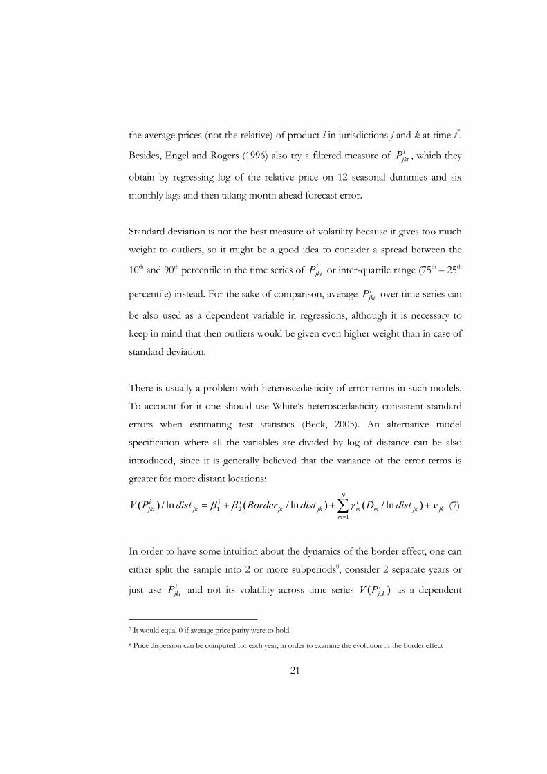
the average prices (not the relative) of product i in jurisdictions j and k at time t7.
Besides, Engel and Rogers (1996) also try a filtered measure of ijktP , which they
obtain by regressing log of the relative price on 12 seasonal dummies and six
monthly lags and then taking month ahead forecast error.
Standard deviation is not the best measure of volatility because it gives too much
weight to outliers, so it might be a good idea to consider a spread between the
10th and 90th percentile in the time series of ijktP or inter-quartile range (75th – 25th
percentile) instead. For the sake of comparison, average ijktP over time series can
be also used as a dependent variable in regressions, although it is necessary to
keep in mind that then outliers would be given even higher weight than in case of
standard deviation.
There is usually a problem with heteroscedasticity of error terms in such models.
To account for it one should use White’s heteroscedasticity consistent standard
errors when estimating test statistics (Beck, 2003). An alternative model
specification where all the variables are divided by log of distance can be also
introduced, since it is generally believed that the variance of the error terms is
greater for more distant locations:
jk
N
mjkm
imjkjk
iijk
ijkt vdistDdistBorderdistPV +++= ∑
=121 )ln/()ln/(ln/)( γββ (7)
In order to have some intuition about the dynamics of the border effect, one can
either split the sample into 2 or more subperiods8, consider 2 separate years or
just use ijktP and not its volatility across time series )( ,
ikjPV as a dependent
7 It would equal 0 if average price parity were to hold.
8 Price dispersion can be computed for each year, in order to examine the evolution of the border effect

22
variable in the basic regression following Parsley and Wei (2001). Regressions for
two periods should be run and then the size of border dummies received from
these two regressions must be compared.
Robustness of the results can be insured through a split of the sample or
exclusion of several periods or goods from it. Where to split the sample and
which periods and goods to exclude depends on the individual characteristics of
the data set under consideration. For instance, 3 separate pooled regressions can
be run for food products, nonfood products and services. Then obtained
estimates should be compared with the results for full sample, and if there are no
substantial differences one can conclude about the robustness of the results.
I suggest a number of modifications to the standard methodology. First of all, I
try to augment the model with several additional explanatory variables in order to
find the influence of different factors on the relative price volatility and
disentangle various determinants of the border effect. For example, I introduce
wage volatility9 into the regression to test a hypothesis that labor market
segmentation explains a part of the border effect. To control for possible pricing-
to-market behavior of the firms I include variability of gross added value per
capita in regression because it can be a proxy for the differences of people’s
wealth across oblasts, which in turn influence consumers’ willingness to spend
certain amount of money on a particular product.
Apart from that, I add some social and political explanatory variables in the
regression. For example, introduction of the relative percentage of people who
voted for Yushchenko in 2004 (or for pro-Yushchenko parties in 2006) into the
model may reveal whether political preferences play a direct role in explaining
9

23
price dispersion across the East and the West of Ukraine. Use of relative
percentage of Russian-speaking people as another explanatory variable would
allow to control for the impact of language differences on the price discrepancy
between the Eastern and the Western Ukraine.
Besides, I try using the common administrative border dummy, which takes the
value of 1 whenever two locations have a common administrative (oblast) border
and 0 otherwise as explicative variable because neighboring oblasts are likely to
have less variation of prices. Finally, a large Dnipro river flows through Ukraine
dividing it in half, so it seems reasonable to control for possible ‘river’ effect
through introduction of respective dummy into the regression.
Within the border effect framework I also examine 205 different possible East-
West divisions, which I generated myself from the map of Ukraine, in order to
find ‘true’ economic border from the data. I simply run 205 pooled regressions
for each of these borders with correspondent border dummy, and find which
border has the largest effect on relative price variation10.
10 I look at coefficients of significant border dummies in different pooled regressions and find which of them
has the largest size relatively to distance

24
C h a p t e r 4
DATA DESCRIPTION
The main data I use for the purpose of my research are monthly average retail
prices of different consumer products across the oblasts, which allow me to
compute relative price volatility. They come from official sources, namely
statistical collections ‘Average Prices and Tariffs for Consumer Goods and
Services’ published by the State Committee of Statistics. I have these collections
available for the period from 1997 to 2004. They provide monthly average prices
of 29 food products, 35 nonfood products and 21 services across 24 oblasts of
Ukraine and Autonomous Republic of Crimea. These are actual prices including
indirect taxes such as tax on added value (VAT) and excise tax. Price information
is collected in oblast and rayon centers, which are chosen taking into account
quantity of urban population and satiation of consumer markets with goods and
services. In order to compute average prices, price data are weighted on the share
of the urban population.
Goods and services for which price data are collected are chosen directly by the
representatives of the regional offices of the State Committee of Statistics
according to demand for them, representation on the consumer market and
regularity of availability for sale during a long period of time. Prices are registered
in the trading network excluding markets and enterprises in the sphere of
services. These prices are also used to compute indices of consumer prices.

25
Classification of products in my price data set is given in Table 1. The number in
brackets indicates the number of products in each category. (See also Appendix B
for a detailed description of the price data)
Table 1. Classification of products
Food products (29) Farinaceous foods (3) Wheat bread, rye bread, bun Cereals (4) Rice, semolina, buckwheat, oats Meet (7) Beef, pork, poultry, lard, smoked sausage, boiled
sausage, herring Dairy products (4) Butter, milk, sour cream, hard cheese Vegetables (5) Potatoes, cabbage, onions, beets, carrots Drinks (2) Vodka, mineral water Other (4) Flour, sugar, sunflower oil, eggs Nonfood products (35) Clothes (13) Man’s suit, man’s shirt, man’s trousers, woman’s
skirt, children’s tracksuit, children’s jacket, children’s dress, children’s t-shirt, rompers, sweater, man’s socks, woman’s stockings, children’s stockings
Footwear (3) Man’s boots, woman’s boots, children’s boots Hygiene products (3) Household soap, toilet-soap, toothpaste Drugs (3) Vessel widening medicine, aspirin, antibiotics Household appliances (2) TV set, refrigerator Furniture (3) Sofa, writing-table, kitchen table Building materials (3) Bricks, cement, wallpapers Fuel (2) Petrol, diesel fuel Other (3) Wool cloth, sheet, exercise-book Services (21) Hairdresser’s (3) Man’s haircut, woman’s haircut, hair curling Cleaning (2) Dry-cleaning, laundry Sewing (2) Trousers sewing, dress sewing Repair services (3) Man’s trousers repair service, shoes repair service,
watch repair service Transportation (2) Freight transportation, parking fee Institutions (5) Theatres, preschool institutions, higher education
institutions, hotels, bath-house Photo services (2) Photos for documents, art photos Other (2) Dental services, video-tape hire

26
The data set of prices I utilize for the purpose of research has several advantages.
First of all, it comes from official sources. Also, it provides average retail prices of
consumer goods, and not price indexes. So, there is no aggregation bias there,
which is usually present in price index data (Ceglowski, 2003). In addition, most
of products are narrowly defined, which also reduces the possibility of bias.
Another advantage of my data is coverage of the wide range of different products
(85 overall). All the investigations that I came across are based on the price data
for much smaller number of products: Engel and Rogers (1996) has 14 different
groups of products, Parsley and Wei (2001) – 27, Beck (2003) – 8, Ceglowski
(2003) – 45, etc. Having average price data for 25 oblasts I can obtain 300 relative
prices for each product. When pooling the data over 85 products I receive cross-
section data set with 25 500 observations.
A weak point of my price dataset is that prices not for all 85 goods and services
are available for the whole period from 1997 till 2004. Due to periodical changes
in classification of the State Committee of Statistics products, for which the
prices are reported, vary slightly from year to year during the considered period.
Some products were added later than 1997, others discontinued to be reported at
some point. For instance, in 2003 the Committee stopped reporting prices of
services at all and reduced the number of reported nonfood goods to only two
(petrol and diesel fuel). Besides, these price data were collected to be used in
computing oblast consumer price indices, and not for inter-oblast comparisons of
the price levels. But despite these more or less minor drawbacks, I make use of
these data for the purpose of my research because this is the only reliable price
data set available in Ukraine.

27
On the basis of available price data I compute relative prices for each product
over 300 oblast pairs, their logs and first difference of logs (see Appendix C).
Table 2 provides short summary statistics for 3 main categories of products.
Table 2. Summary statistics for 3 main product categories
Relative prices Log of relative prices Difference of logs of relative prices Products
Avg Max Min Avg Max Min Avg Max Min Food products 1.041 5.67 0.15 0.0212 1.73 -1.90 -0.00005 1.63 -1.85Nonfood products 1.074 9.63 0.13 0.0320 2.26 -2.04 0.00113 2.26 -2.04Services 1.130 6.00 0.14 0.0430 1.79 -1.97 0.00170 1.54 -1.74
According to Table 1, relative prices of food products on average are most close
to 1, of services – least close and of nonfood products – somewhere in the
middle. Most of services are non-tradable, which explains why on average their
relative prices diverge the most from 1. However, from the perspective of
tradability one would expect absolute PPP to hold the best for nonfood products
and, consequently, their prices to be the closest to 1, since food products are
perishable goods, which puts some restriction on their tradability. But, on the
other hand, nonfood products are much more heterogeneous than food, which
can ration higher variability of their prices. It is probably also due to
differentiation of nonfood products that the range between their maximum and
minimum relative prices is the highest among product categories.
If to look at the first difference of logged relative prices, one can see that its
average value for food products negligibly deviates from zero, whereas for
nonfood products and services the correspondent values are more than an order
of magnitude higher. This suggests that relative PPP also holds best for food
products. At the same time, the range between maximum and minimum values is
the smallest for services, which might results from lower responsiveness to
different short-term shocks.

28
Then, I consider separately percentage differences of the products’ absolute and
relative prices11 for oblast pairs in which both oblasts are located in the East
(East-East), in the West (West-West) and for those pairs in which one oblast is in
the East and the other is in the West (East-West). Summary of results is
presented in the table below (for results for all 85 products see Appendix D).
Table 3. Average standard deviation of percentage differences of absolute and relative prices Average prices Relative prices
East-West
East-East
West-West
East-West
East-East
West-West
Food products 0.12702 0.11185 0.12071 0.08484 0.07592 0.08678Nonfood products 0.11999 0.11836 0.12021 0.08227 0.07712 0.08789Services 0.08655 0.07993 0.08964 0.09085 0.07796 0.08037All the products 0.11413 0.10664 0.11283 0.08527 0.07692 0.08565
If the East-West border did not matter, then average percentage differences of
average and relative prices would be the same for the East-West, East-East and
West-West pairs of oblasts. In our case, average percentage differences both for
absolute and relative prices are the highest for oblast pairs located in the West,
and the lowest for oblast pairs located in the East. Cross-border pairs are in the
middle. One would expect price volatility to be higher in the West because
Eastern and Western regions according to our classification are not symmetric:
the West comprises of almost twice as many oblasts as the East (16 and 9
respectively). Therefore, there are 120 oblast pairs in the West and only 36 in the
East. It is more difficult to explain why price volatility for the Western oblast
pairs is a little higher than for cross-border pairs. In the paper of Engel and
Rogers (1996) intra-national price volatility between the US states for some
categories of products was also higher than US-Canada cross-border volatility.
11 Logs of relative prices and first differences of logs of relative prices respectively
29
They explained it by high product differentiation of some products and the fact
that there are products, which both Canada and the US mostly import from some
third countries.
I also constructed 4 hypothetical baskets of consumer products: first basket
comprising 29 food products, second – 35 nonfood products, third – 21 services
and forth – all 85 products. To do this I first found the average price of each
good in each oblast during the period for which price data of this particular
product is available12. Then, I used rather primitive construction procedure
simply giving all the products in each basket equal weights. It obviously does not
have to correspond to reality. Still it allows to make a rough judgment about
deviations of price levels across the oblasts. Figure 1 illustrates the results for the
basket of all 85 products (see Appendix E for all 4 baskets).
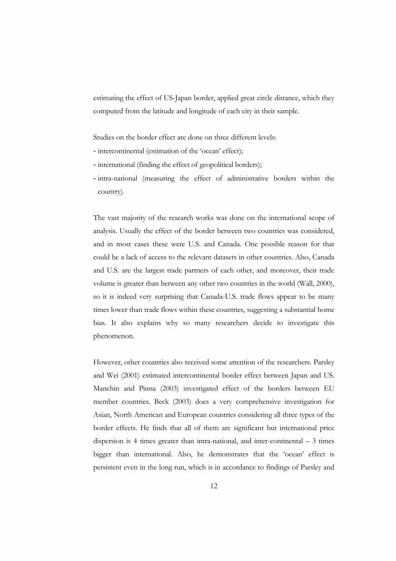
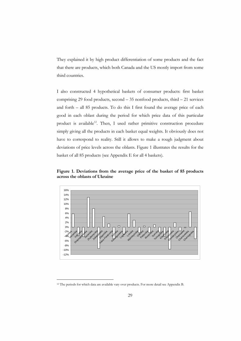
Figure 1. Deviations from the average price of the basket of 85 products across the oblasts of Ukraine
-12%
-10%
-8%
-6%
-4%
-2%
0%
2%
4%
6%
8%
10%
12%
14%
16%
Crimea
Vinnytsk
a
Volyns
ka
Dniprope
trovs
ka
Donetsk
a
Zhytomyrs
ka
Zakarpa
tska
Zapo
rizka
Ivano-F
rankivs
ka
Kyivsk
a
Kirovo
gradska
Lugan
ska
Lvivsk
a
Mykolay
ivska
Odesk
a
Poltav
ska
Rivnens
ka
Sumsk
a
Ternopilsk
a
Kharki
vska
Kherso
nska
Khmeln
ytska
Cherkas
ka
Chernive
tska
Chernigi
vska
12 The periods for which data are available vary over products. For more detail see Appendix B.

30
The average price of basket consisting 85 products during 1997-2004 was the
highest in Crimea, Dnipropetrovska, Donetska, Luganska and Chernivetska
oblasts, all but 1 of which are in the East. It was the lowest in Vinnytska,
Volynska, Zhytomyrska, Ivano-Frankivska, Kirovogradska, Ternopilska,
Kharkivska and Chernigivska oblasts, all but 1 of which are in the West. So, price
level is generally higher in the Eastern Ukraine and lower in the Western, which is
also shown in Figure 2.
Figure 2. Deviations from the average price of 4 baskets of products in the East and the West of Ukraine
-8%-6%-4%-2%0%2%4%6%8%
10%12%
Foodproducts
Nonfoodproducts
Services Allproducts
EastWest
For all 4 baskets of products prices in the East were higher and in the West lower
than on average in Ukraine. The biggest difference in price levels between the
East and the West is observed for services in line with their non-tradability. In
Figure 2 price discrepancy for nonfood products is a little lower than for food,
somewhat contrary to figures reported in Table 2 but in accordance with higher
tradability of nonfood products, which are non-perishable goods.

31
Apart from the price data, I also make use of some complementary data for my
analysis, which are:
- 300 distances between the oblast capital cities;
- monthly data of average wages across oblasts during 1999-2004;
- average gross added value during 1997-2004 across oblasts;
- percentage of people who voted for Yushchenko and Yanukovych during
Presidential elections 2004 across oblasts;
- percentage of people who voted for pro-Yushchenko and pro-Yanukovych
parties during Parliamentary elections 2006 across oblasts;
- share of Russian-speaking people across oblasts according to All-Ukrainian
Census 2001.
These data also come from official sources, namely:
- different statistical collections of the State Committee of Statistics;
- report of All-Ukrainian Census in 2001;
- reports of the Central Election Committee.
I
On average, distance between the oblast capital cities is around 594 km. It is
almost equal for oblast pairs in the East and in the West: 410 and 449 km
respectively. For cross-border oblast pairs this figure is 762 km.
It is also worth to compare average wages across Ukrainian oblasts, since they
reflect price of the labor, which is an important factor of production of goods
and services. Figure 3 is a counterpart to Figure 1 for wages. It demonstrates
deviations from the average level of wages across Ukrainian oblasts (see also
Appendix F for summary statistics of the wage data).

32
Figure 3. Deviations from the average level of wages across the oblasts of Ukraine
-150%
-120%
-90%
-60%
-30%
0%
30%
60%
90%
120%
150%
Crimea
Vinnyts
ka
Volynsk
a
Dniprop
etrovs
ka
Donets
ka
Zhytomyrs
ka
Zakarpa
tska
Zapori
zka
Ivano
-Fran
kivsk
a
Kyivsk
a
Kirovo
grads
ka
Luga
nska
Lvivs
ka
Mykola
yivsk
a
Odesk
a
Poltav
ska
Rivnen
ska
Sumsk
a
Ternop
ilska
Kharki
vska
Kherso
nska
Khmeln
ytska
Cherka
ska
Cherni
vetsk
a
Cherni
givska
Deviations of wages are an order of magnitude higher than of prices, which is
expected because labor is not as mobile as products. Wage deviations range from
about -130% to +130%, whereas the spread of price discrepancy is (-10%;
+13%). 15 out of 25 oblasts have the same sign of deviations for prices and
wages, and among those that have different signs most oblast have deviations
rather close to zero. Overall, the highest wages during 1999-2004 were observed
in Dnipropetrovska, Zaporizka, Kyivska, Luganska, Mykolayivska and Sumska
oblasts, all of which but Kyivska are located in the Eastern Ukraine. The lowest
wages had Volynska, Zhytomyrska, Ivano-Frankivska and Lvivska oblasts, all of
which are in the Western Ukraine. So, both wages and prices were generally
higher in the East than in the West over the period of 1999-2004. To be precise,
wages in the East were about 44% higher and in the West 27% lower than on
average in Ukraine.

33
I would like to conclude the data description section by a correlation matrix that
presents degrees of correlation between average price level13, wage, gross added
value per capita, percentage of Russian-speaking people and those who voted for
Yanukovych at the Presidential elections 2004 and East dummy14 for the oblasts
of Ukraine.
Table 4. Correlation matrix of some indicators across the oblasts of Ukraine Price
level Wage Gross added value per capita
Russian-speaking Yanukovych East
dummy Price level 1 Wage 0.48 1 Gross added value per capita 0.28 0.89 1
Russian-speaking 0.43 0.72 0.51 1
Yanukovych 0.40 0.74 0.55 0.94 1 East dummy 0.39 0.72 0.54 0.87 0.91 1
The main message of this matrix is that there is a substantial positive correlation
between all these indicators. They have higher values in the East than in the West,
which was earlier shown explicitly for prices and wages. This suggests that if in
the empirical part I find a significant border effect between the East and the West
it may reflect either economic (wage, gross added value per capita), or political, or
linguistic differences, or possibly, some other factors. To check the role of each
of these indicators, they will have to be introduced one way or another into the
model.
13 I proxy it to the price of the basket of 85 products that I constructed earlier
14 Takes on value 1 whenever oblast is in the East according to the political division, and 0 otherwise

34
C h a p t e r 5
EMPIRICAL EVIDENCE
I start empirical part with analysis of the regression pooled over all 85 products.
This gives me 2550015 observations and, therefore, a lot of degrees of freedom,
which insures high precision of the estimates.
I first run a pooled regression (3) from the methodology section, which has
exactly the same form as the baseline model offered initially by Engel and Rogers
(1996): jk
N
mmm
K
iiijkjkjkt uDGBorderdistPV ++++= ∑∑
−
==
1
1121 ln)( γλββ , with
first difference of logs of relative prices as a dependent variable and log of
distance, border dummy16, 85 product dummies and 24 oblast dummies17 as
explicative variables. I use White’s heteroscedasticity-consistent standard errors,
since variance of the error terms is likely to have positive correlation with
distance between the locations. Short summary of the results is presented in the
table below.
Table 5. Summary of Stata output for regression (3)
Variable Coefficient Robust Std. Error t P>|t| 95% Confidence
Interval Lndist .0017601 .0006812 2.58 0.010 .0004249 .0030953 Border .0030536 .0007297 4.18 0.000 .0016233 .0044839
15 85*300(number of oblast pairs)=25500
16 For East-West political border
17 One oblast dummy has to be excluded to avoid perfect collinearity. I excluded dummy for Chernigiv oblast

35
For this particular regression coefficients of both natural log of distance and
border dummy are highly significant. Both of them are greater than zero, which
corresponds to theoretical predictions, since one would expect price dispersion to
be higher for more distant oblasts and those separated by a border. According to
the results of regression, increase of distance between oblasts by 1% raises price
dispersion by 1.76%.
Economic significance of the border can be computed according to the formula
proposed by Parsley and Wei (2001):
)1)(exp(*1
2 −= ββdistZ =762*exp(0.0030536/.0017601)-1)=560 km, which is
negligibly small value in comparison with findings of Engel and Rogers (1996),
who estimated the effect of Canada-US border to be equivalent to 75000 miles.
R-squared for this regression equals to 0.7724, so the model has rather high
explanatory power. Coefficients of all 85 product dummies are highly significant
(p-value = 0.000), suggesting that price volatility has some important product-
specific features. 21 out of 24 oblast dummies18 are significant at 5% level of
significance, which means that oblast-specific characteristics also have substantial
impact on price dispersion. For instance, some oblasts might have more
integrated markets with the rest of Ukraine than the other. Then, price volatility
for oblast pairs containing these oblasts would be lower on average, and vice
versa. In a given regression oblast pairs that include either Kirovogradska, or
Ternopilska, or Cherkaska oblasts appeared to have price dispersion above mean.
18 To save space, I do not provide Stata output for 85 product dummies and 24 product dummies.
Henceforth only results for the variables of special interest are provided.

36
If to run regression (3) but exclude border dummy from it, R-squared will remain
essentially the same but the coefficient of logged distance will be twice as high as
in the original regression. This will happen because now the coefficient will show
not only the effect of distance but also, implicitly, effect of the border – omitted
variable in this specification. Even in the original regression (3) there could be a
misspecification bias because historical borders and/or Dnipro River might also
matter for the magnitude of price dispersion between the oblasts in Ukraine.
Besides, oblasts that share common border might have lower relative price
volatility. So, next I will run regression (3) augmented by historical and common
border dummies and the Dnipro River dummy.
I constructed the Dnipro River dummy the way that it takes on value 1 any time
oblast pair contains oblasts located on different sides of the Dnipro River, and 0
if they are located on the same side. However, there are some oblasts
(Dnipropetrovska, Kyivska, Khersonska and Cherkaska), which are crossed by
the Dnipro river in the middle. I assume that in these oblasts the river effect is
already incorporated in the intra-oblast price dispersion, so for pairs containing
these oblasts the Dnipro River dummy always equals to zero.
From a theoretical standpoint, I would expect coefficients of the historical border
and Dnipro dummies to be positive, and of common border dummy – negative.
These predictions hold for coefficients of Dnipro and common border dummies
but not of historical border. But, actually, it is not very important, since all of
them are insignificant anyway. So, no evidence that the regression (3) has
misspecification bias is found so far.
Running regression (4) with quadratic specification of distance proves concave
relationship of distance: coefficient of distance is positive and statistically
significant at 5% level of significance, and coefficient of squared distance –

37
negative and significant at 10% level. Border dummy coefficient remains positive
and highly significant in this specification.
Table 6. Summary of Stata output for regression (4)
Variable Coefficient Robust Std. Error t P>|t
| 95% Confidence
Interval Distance 9.57e-06 4.06e-06 2.36 0.018 1.62e-06 .0000175 Dist-sqr -5.11e-09 3.06e-09 -1.67 0.095 -1.11e-08 8.97e-10 Border .0031926 .0007576 4.21 0.000 .0017078 .0046775
Controlling explicitly for heteroscedasticity (running regression (7):
jk
N
mjkm
imjkjk
iijk
ijkt vdistDdistBorderdistPV +++= ∑
=121 )ln/()ln/(ln/)( γββ )
does not alter general results. Coefficient of the border dummy remains
significant and approximately of the same size (0.003412).
Since most of 24 oblast dummies are statistically significant in all the mentioned
specifications, I find it reasonable to try to include in the model 299 dummies for
all but one oblast pairs. The rationale is that if oblast-specific features influence
substantially price dispersion, then, possibly, oblast pair-specific features also do.
Inclusion of 299 more explicative variables is not going to hurt degrees of
freedom too badly because I have very large number of observations – 25500.
But after all I find out that coefficients of only about a dozen out of 299 oblast
pair dummies are significant at 5% level of significance, and just one – at 1%
significance level.
Up till now I was conducting my analysis using just one measure of price
volatility, namely standard deviation of the first difference of logs of relative
prices. But it is worthwhile to consider also 7 other price volatility measures
mentioned in the section on methodology, namely:

38
- standard deviation of )log(,
,itk
itj
PP
(volatility2);
- spread between 10th and 90th percentile of ijktP , where
)log()log(1,
1,
,
,itk
itj
itk
itji
jkt PP
PP
P−
−−= (volatility 3) or )log(,
,itk
itj
PP
(volatility 4);
- inter-quartile range of ijktP (volatility 5 and 6);
- mean ijktP (volatility 7 and 8).
I duplicated main points of my analysis for these volatility measures. Short
summary of results can be found in the table below.
Table 7. Main Stata output for specification (3) with volatility 2 to 8 as a dependent variable
Variable Coefficient Robust Std. Error t P>|t| 95% Confidence
Interval Volatility 2 (R-sqr = 0.8259) Lndist .0053094 .0007702 6.89 0.000 .0037998 .0068191Border .0010746 .0008894 1.21 0.227 -.0006686 .0028178Volatility 3 (R-sqr = 0.8938) Lndist .003103 .0006455 4.81 0.000 .0018377 .0043682Border .0003144 .0007991 0.39 0.694 -.0012519 .0018807Volatility 4 (R-sqr = 0.8315) Lndist .0150636 .0018978 7.94 0.000 .0113438 .0187834Border .001789 .0022003 0.81 0.416 -.0025238 .0061018Volatility 5 (R-sqr = 0.9074) Lndist .0014993 .0002471 6.07 0.000 .0010151 .0019835Border .0000591 .000304 0.19 0.846 -.0005366 .0006549Volatility 6 (R-sqr = 0.7646) Lndist .008711 .0012356 7.05 0.000 .0062892 .0111327Border .0013757 .0015331 0.9 0.370 -.0016294 .0043807Volatility 7 (R-sqr = 0.0485) Lndist .0000294 .0001804 0.16 0.871 -.0003242 .0003829Border .0005355 .0002217 2.41 0.016 .0001008 .0009701Volatility 8 (R-sqr = 0.0821) Lndist -.0032037 .0031969 -1 0.316 -.0094698 .0030624Border .0208572 .0039093 5.34 0.000 .0131948 .0285196

39
As noted in section on methodology, measures of volatility 3-6 ignore outliers,
whereas volatilities 7-8 give them rather high weigh. According to Table 7, for all
the volatilities ignoring outliers R-squared is rather high, log of distance has big
explanatory power, whereas political border appears to be insignificant. For
volatilities which take outliers into account the situation is the opposite. Quite
logically, R-squared is very small for them because outliers usually reflect some
shocks. However, it is a bit surprising that logged distance has no substantial
impact on them, whereas border is important.
For regressions with volatilities 2-6 as dependent variables the Dnipro River,
historical and common border dummies were insignificant. However, for
volatilities 7-8 common border dummy becomes highly significant (p-value =
0.001 and 0.000 respectively) and has negative sign as expected, since oblasts that
have a common border are supposed to have more integrated markets and,
therefore, lower price dispersion. Roughly 95% of all product dummies and 75%
of oblast dummies are significant for all these volatility measures, so product-
specific and oblast-specific effects repeatedly prove to be important.
The analysis of different volatilities has already shown that the results obtained
from regression (3) are not robust, so there is not much sense to present any
other check on robustness like split of the sample or exclusion of some products.
I proceed further by testing the importance of wage volatility, differences in the
average gross added value per capita, percentage of people who voted for
Yushchenko in 2004 and share of Russian-speaking population in explaining
price dispersion across oblasts.
For the analysis of the impact of wage volatility on price dispersion I use two
different ways to compute wage volatility, which are essentially counterparts to

40
the first and second measures of price volatility: standard deviation of ijktw , with
)log()log(1,
1,
,
,itk
itj
itk
itji
jkt ww
ww
w−
−−= (wage volatility 1) or )log(,
,itk
itj
ww
(wage volatility 2).
Since there are differences in periods for which price data for various products
are available, as stated in ‘Data description’ section, I compute separately
measures of wage volatility correspondent to each product and then pool them
over all the products. However, some disparities can not be eliminated because
price data for 30 out of 85 products are available starting from 1997, whereas
wage data are available only from 1999.
After computing wage volatilities I run two pooled regression of the general
form:
jk
N
mmm
K
iiijktjkjkjkt uDGwVBorderdistPV +++++= ∑∑
−
==
1
11321 )(ln)( γλβββ
In pooled regression 1 with )log()log(1,
1,
,
,itk
itj
itk
itji
jkt PP
PP
P−
−−= and
)log()log(1,
1,
,
,itk
itj
itk
itji
jkt ww
ww
w−
−−= coefficient of wage volatility is statistically
significant at 5% level of significance but surprisingly has a negative sign. In
pooled regression 2 it is insignificant. These unexpected results could be partly
due to lack of correspondence between the periods for which price volatility and
wage volatility are computed as mentioned above.
To test the significance of differences in political and linguistic preferences, I use
data on percentage of people who voted for Yushchenko at Presidential elections
2004 and percentage of people who consider Russian their native language to

41
compute differences for all oblast pairs. This allows me to receive two explicative
variables – proxies of political and linguistic preferences. I add them to model (3)
and run 8 pooled regressions with different measures of price volatility.
Differences in political preferences appear to have no direct impact on the price
dispersion, since coefficient of this variable is insignificant in all 8 specifications.
A possible explanation can be that political preferences in reality are important
but have to enter regression in a different functional form.
There is some evidence, however, about positive influence of differences in
linguistic preferences on price dispersion. Its coefficient is positive and
statistically significant for specifications with volatilities 6, 7 and 8. This
corresponds to theoretical predictions and means that the more different are two
oblasts according to language preferences, the higher price dispersion one might
expect for them. Besides, native language might reflect person’s origin and,
therefore, some cultural differences, including preferences what products to
consume.
Table 7. Testing for significance of linguistic differences
Variable Coefficient Robust Std. Error t P>|t| Language (volatility 6) .0170623 .0013244 2.05 0.040 Language (volatility 7) .0033063 .0012093 2.73 0.006 Language (volatility 8) .0796957 .021798 3.66 0.000
Analysis of variation in gross added value per capita across oblasts, which can be
used as a proxy for income and wealth, also produces some interesting results.
This variable appeared to be significant in 4 out of 8 pooled regressions and
always higher than zero. This means the more different are two oblasts in terms
of wealth the higher price dispersion can be expected for the them. It can also
potentially mean pricing-to-market behavior of the firms.

42
Variable Coefficient Robust Std. Error t P>|t| Relative GAV per capita (volatility 1)
.002171 .0012135 1.79 0.074
Relative GAV per capita (volatility 3)
.0023648 .0010939 2.16 0.031
Relative GAV per capita (volatility 7)
.0056722 .0003312 17.13 17.13
Relative GAV per capita (volatility 8)
.1711945 .0058568 29.23 0.000
I also run simple OLS regressions for each of 85 products separately with
volatility 1 and volatility 2 as dependent variables. This brings the following
results (see Appendix H2 for more detail):
I. For volatility 1:
- logged distance is positive and significant19 for 14 food products, 2
nonfood products and 4 services;
- political border is positive and significant for 6 food products, 3 nonfood
products and 9 services;
- historical border is positive and significant for 3 food products, 5
nonfood products and 1 service;
- common border is negative and significant for 4 food products, 1
nonfood product and 2 services;
- Dnipro River is positive and significant for food products, 3 nonfood
products and no services.
II. For volatility 2:
- Logged distance is positive and significant for 18 food products, 6
nonfood products and 1 service;
19Significant stands for significant at 10% level of significance in the analysis of separate OLS regressions for each product

43
- political border is positive and significant for 12 food products, 3
nonfood products and 3 services;
- historical border is positive and significant for 3 food products, 5
nonfood products and 2 services;
- common border is negative and significant for 1 food product, no
nonfood products and no services;
- Dnipro River is positive and significant for 4 food products, 2 nonfood
products and 2 services.
So, separate OLS regressions for 85 products do not give strong evidence on the
border effect.
Running pooled regressions with standard deviation of ijktP as a dependent
variable ( )log()log(1,
1,
,
,itk
itj
itk
itji
jkt PP
PP
P−
−−= in specification 1 and )log(,
,itk
itji
jkt PP
P = in
specification 2 allows drawing the following conclusions (see Appendix C1 for
Stata output of selected pooled regressions): distance is highly significant in both
specifications;
- political border is highly significant in specification 1 but not in specification
2;
- historical border is statistically insignificant in both specifications20;
- common border dummies are statistically insignificant in both specifications;
- around 95% of oblast dummies are highly significant in both specifications;
20 Inclusion both political and historical border dummies into regression simultaneously does not change the
results

44
- around 80% of product dummies are highly significant in both specifications;
- river dummies are statistically insignificant in both specifications.
Adjusted R2 equals about 0.7723 in specification1 and about 0.8259 in
specification2. Introduction of the border dummy into regression does not
increase adjusted R2 substantially but reduces the size of the distance coefficient.
I also tried running pooled regressions with quadratic specification of distance. It
did not influence the results.
Running simple OLS regressions for each of 85 products separately brought the
following results (see Appendix C2):
III. Specification 1:
- distance is positive and significant for 20 food products, 4 nonfood
products and 16 services;
- political border is positive and significant for 5 food products, 3 nonfood
products and 8 services;
- historical border is positive and significant for 3 food products, 1
nonfood product and 4 services;
IV. Specification 2:
- distance is positive and significant for 19 food products, 4 nonfood
products and 1 service;
- political border is positive and significant for 9 food products, 2 nonfood
products and 2 services;
- historical border is positive and significant for 2 food products, 3
nonfood products and 1 service.
This does not provide strong evidence for the border effect in Ukraine, since
coefficient of the East-West border is insignificant in most of separate OLS
regressions for 85 products. However, it demonstrates that the effect of this

45
border on the price dispersion is larger than of historical border, common
borders and Dnipro River.
I also tried finding the ‘true’ East-West border suggested by data. In order to do
this, I generated 205 potentially possible East-West divisions from the map of
Ukraine. Then, I created correspondent border dummies, and ran regression (3)
for 8 different measures of price volatility and 205 different East-West border
dummies (1640 regressions in total). I found borders, which were significant and
had the highest values for most of these 8 price volatilities. According to this
analysis, the political border was among the best candidates for the ‘true’ East-
West border.

46
C h a p t e r 6
CONCLUSIONS
There is some evidence that political border has a positive impact on the price
dispersion across the oblasts of Ukraine but its economic significance is not very
high. When converted into distance units this border is equivalent to about 560
kilometers, which is rather low figure in comparison with findings of other
researchers for other countries.
Not all of the measures of price volatility reveal positive and significant border
effect, so the results are not robust. Still, the political border appears to have
much higher explanatory power of the price dispersion than historical border,
common borders between oblasts, the Dnipro River and wage volatility.
Moreover, political border is a good candidate for the ‘true’ East-West border of
Ukraine according to actual data. So, its role definitely should not be ignored.
However, some fixed product-specific and oblast-specific features explain much
larger part of the price volatility, which suggests that Ukrainian markets are more
segmented by product and oblast than by hypothetical ‘East-West’ border.
Distances between locations, which approximate well shipping costs, are also
consistently proven to have a positive effect on the price dispersion.
Also, differences in the linguistic preferences and gross added value per capita
appear to matter for price volatility across the oblasts of Ukraine. The impact of
the former could reflect people’s heterogeneity by origin, which influences their
consumption preferences. Both are likely to be connected to the pricing-to-

47
market behavior of the firms, which implies that Ukrainian markets are not very
competitive.
These findings can have some important policy implications for Ukrainian
government:
- language issues should be given more attention, since they matter not
only from the social and political perspectives but also have some
economic meaning;
- economic competition policies must be reviewed and improved to insure
the competitive environment and lack of opportunities for pricing-to-
market behavior of the firms.
However, the evidence of economic nature of the East-West political border
does not seem strong enough to support the need of transforming Ukraine into
the federal state.

48
BIBLIOGRAPHY
Anderson J. (2000) Why Do Nations Trade (So Little)? Pacific Economic Review, vol. 5, p. 115-134. Anderson M. and S. Smith (1999a) Do National Borders Really Matter? A Reconsideration of Canada-U.S. Regional Trade Review of international economics, vol. 7, p. 219-227 Anderson M. and S. Smith (1999b) Canadian Provinces in World Trade: Engagement and Detachment Canadian Journal of Economics, vol. 32, p. 22-38. Beck, G. (2003) Nominal Exchange Rate Regimes and Relative Price Dispersion: On the Importance of Nominal Exchange Rate Volatility for the Width of the Border. CFS Working Paper Series 2003/45. Ceglowski, J. (2003) Law of One Price: Intranational Evidence for Canada. Canadian Journal of Economics, vol. 36(2), p. 373-400. Combes, P., M. Lafourcade and T. Mayer (2003) Can Business and Social Networks Explain the Border Effect Puzzle? Working Papers 2003-02, CEPII research center.
Duvereux, M. and C. Engel (1998) Fixed vs. Floating Exchange Rates: How price setting affects the optimal choice of exchange rate regime. NBER Working Paper No. 6867.
Engel, C. and J. Rogers (1996) How Wide Is the Border? American Economic Review, vol. 86(5), p. 1112-1125.
Engel, C. and J. Rogers (2001) Violating the Law of One Price: Should We Make a Federal Case Out of It? Journal of Money, Credit and Banking, vol. 33(1), p. 1-15. Galushko, V. (2003) Has Spatial Market Integration Increased Over Time: The Evidence From Ukrainian Food Markets? EERC MA Thesis. Frankel J. and A. Rose (1996) A Panel Project on Purchasing Power Parity: Mean Reversion within and between Countries Journal of International Economics, vol. 40(1), p. 209-224. Fukao, K. and T. Okubo (2004) Why Has the Border Effect in the Japanese Market Declined?: The Role of Business Networks in East Asia Hi-Stat Discussion Paper Series d03-24.

49
Gorodnichenko, Y. and L. Tesar (2005) A Re-Examination of the Border Effect. NBER Working Papers 11706.
Head K. and T. Mayer (2002) Illusory Border Effects: Distance Mismeasurement Inflates Estimates of Home Bias in Trade Working Papers 2002-01, CEPII research center.
Helliwell, J. (1996) Do National Borders matter for Quebec’s Trade? Canadian Journal of Economics, vol. 29, p. 507-522. Helliwell, J. (1998) How Much Do National Borders Matter? DC: Brookings Institutional Press.
Isard, P. (1977) How Far Can We Push the “Law of One Price”? American Economic Review, vol. 67(5), p. 942-948.
Manchin M. and A. Pinna (2003) Border effects in the enlarged EU area. Working Paper CRENoS 200301. McCallum, J. (1995) National Borders Matter: Canada-U.S. Regional Trade Patterns. American Economic Review, vol. 85, p. 615-623. Obstfeld, M. and K. Rogoff (2000) The Six Major Puzzles in International Economics: Is There a Common Cause? NBER Macroeconomics Annual
Parsley, D. and S. Wei (1996) Convergence of the Law of One Price without Trade Barriers or Currency Fluctuations. Quarterly Journal of Economics, vol. 111(4), p. 1211-1236.
Parsley, D. and S. Wei (2001) Explaining the Border Effect: The Role of Exchange Rate Variability, Shipping Costs, and Geography. Journal of International Economics, vol. 55(1), p. 87-106. Rogoff, K. (1996) The Purchasing Power Puzzle. Journal of Economic Literature, vol. 34, p. 647-688.
Sagidova, G. (2004) Price Transmission in Grain Market: Case of Ukraine. EERC MA Thesis.
Vashchuk, O. (2003) The Law of One Price and Regional Price Convergence in Ukraine. EERC MA Thesis
Wall, H. (2000). Gravity model specification and the effects of the Canada-U.S. border. Working Papers 2000-024A, Federal Reserve Bank of St. Louis.
Witte, M. (2005) Sticky Prices, a Volatile Exchange Rate and the Border. International trade 0508010, Economics Working Paper Archive EconWPA.

50
Wolf, H. (2000) Intranational Home Bias in Trade. Review of Economics and Statistics, vol. 82(4), p. 555-563.
Yi, K. (2005) Vertical specialization and the border effect puzzle. Working Papers05-24, Federal Reserve Bank of Philadelphia.

2
APPENDIX A. DIFFERENT DIVISIONS OF UKRAINE
A1. Political division
WEST % voted for Yushchenko
in 2004
% voted for pro-Yushchenko parties* in 2006
EAST % voted for Yanukovych
in 2004
% voted for pro-Yanukovych party** in 2006
Vinnytska 84.07% 70.84% Crimea 81.26% 57.92%
Volynska 90.71% 76.99% Dnipropetrovska 61.13% 44.95%
Zhytomyrska 66.86% 54.02% Donetska 93.54% 73.63%
Zakarpatska 67.45% 53.74% Zaporizka 70.14% 51.23% Ivano-Frankivska 95.72% 86.36% Luganska 91.24% 74.27%
Kyivska 82.70% 70.37% Mykolayivska 67.13% 50.35%
Kirovogradska 63.40% 50.51% Odeska 66.56% 47.48%
Lvivska 93.74% 82.12% Kharkivska 68.12% 51.66%
Poltavska 66.00% 55.40% Khersonska 51.32% 39.14%
Rivnenska 84.52% 73.39%
Sumska 79.45% 66.06%
Ternopilska 96.03% 85.55%
Khmelnytska 80.47% 67.22%
Cherkaska 79.10% 67.66%
Chernivetska 79.75% 65.78%
Chernigivska 71.15% 60.31% * Block of Yuliya Tymoshenko, block ‘Nasha Ukrayina’, Socialistic party of Ukraine, block of Kostenko and Plyushch, block ‘Pora-PRP’ ** Party of regions
A2. Historical division
WEST Ivano-Frankivska, Lvivska, Ternopilska, Volynska, Rivnenska, Zakarpatska, Chernivetska
Lands in the Western Ukraine that were joined to Soviet Union in 1944
NORTH-CENTER
Kyivska, Vinnytska, Zhytomyrska, Kirovogradska, Khmelnytska, Cherkaska
The rest of the Right Bank territory of Ukraine that was under Polish control from the time of the Polish-Lithuanian Commonwealth to the Second Partition of Poland in 1793
NORTH-EAST
Chernigivska, Poltavska, Sumska The Left Bank Ukraine that was under Russia during the same period
SOUTH Dnipropetrovska, Zaporizka, Mykolayivska, Odeska, Khersonska, Crimea
The Southern Ukraine which unites historical region of Zaporizhya, former Ottoman Black Sea littoral and the Crimean peninsula
EAST Donetska, Luganska, Kharkivska Eastern regions with heavy industrialization and in-
migration from Russia

3
APPENDIX B. DESCRIPTION OF THE PRICE DATA
B1. Food price data
Product Units Period Product Units Period Wheat bread 1 kg 2003:1-2004:12 Butter 1 kg 1997:1-2004:12 Rye bread 1 kg 1999:1-2004:12 Sunflower oil 1 liter 1997:1-2004:12 Bun 500 g 1999:1-2004:12 Milk 1 liter 1997:1-2004:12 Flour 1 kg 1997:1-2004:12 Sour cream 1 kg 1997:1-2004:12 Rice 1 kg 1997:1-2004:12 Hard cheese 1 kg 1997:1-2004:12 Semolina 1 kg 1997:1-2004:12 Eggs 10-pack 1997:1-2004:12 Buckwheat 1 kg 1999:1-2004:12 Sugar 1 kg 1997:1-2004:12 Oats 1 kg 1999:1-2004:12 Potatoes 1 kg 1997:1-2004:12 Beef 1 kg 1997:1-2004:12 Cabbage 1 kg 1997:1-2004:12 Pork 1 kg 1997:1-2004:12 Onions 1 kg 1997:1-2004:12 Poultry 1 kg 1997:1-2004:12 Beets 1 kg 1997:1-2004:12 Lard 1 kg 1997:1-2004:12 Carrots 1 kg 1997:1-2004:12 Smoked sausage 1 kg 2001:7-2002:12 Vodka (alcohol) 1 liter 1997:1-2004:12 Boiled sausage 1 kg 1999:1-2001:6 Mineral water 1 liter 1997:1-2002:12 Herring 1 kg 1997:1-2004:12
B2. Nonfood price data
Product Units Period Product Units Period Man’s suit 1 item 2001:7-2003:12 Household soap 200 g 1997:1-2002:12 Man’s shirt 1 item 2000:1-2003:12 Toilet-soap 100 g 2001:7-2002:12 Man’s trousers 1 item 1999:1-2001:6 Toothpaste 1 item 2000:1-2001:6 Woman’s skirt 1 item 1997:1-2003:12 Exercise-book 1 item 2000:1-2001:6 Children's tracksuit 1 item 2001:7-2002:12 Vessel widening
medicine 10 pills 2001:7-2002:12
Children's jacket 1 item 1997:1-2003:12 Aspirin, analgin 10 pills 1999:1-2001:6 Children's dress 1 item 2001:7-2003:12 Antibiotics 10 pills 2000:1-2001:6 Children's T-shirt 1 item 2000:1-2001:6 TV set 1 item 2000:1-2003:12 Rompers 1 item 1999:1-2001:6 Refrigerator 1 item 1997:1-2003:12 Sweater, jumper 1 item 2000:1-2002:12 Sofa, bed 1 item 1997:1-2002:12 Man’s socks 1 pair 2000:1-2002:12 Writing-table 1 item 2001:7-2002:12 Woman’s stockings 1 pair 1997:1-2002:12 Kitchen table 1 item 2000:1-2001:6
Children's stockings 1 pair 1997:1-2002:12 Bricks 1000
items 2000:1-2001:6
Man’s boots 1 pair 1997:1-2003:12 Cement 50 kg 2001:7-2002:12 Woman’s boots 1 pair 1997:1-2003:12 Wallpapers 10 m 2001:7-2003:12 Children's boots 1 pair 2000:1-2002:12 Petrol 1 liter 1999:1-2004:12 Wool cloth 1 m 2000:1-2001:6 Diesel fuel 1 liter 2002:1-2004:12 Sheet 1 item 2000:1-2001:6

4
B3. Services price data
Product Units Period Product Units Period
Dry-cleaning 1 item 2000:1-2002:12 Watch repair service 1 item 2000:1-2001:12Laundry and ironing 1 kg 1997:1-2002:12 Parking fee 24 hours 2000:1-2001:12
Bath-house service 1 hour 2000:1-2002:12 Freight transportation 1 service 2002:1-2002:12Man's haircut 1 service 1997:1-2002:12 Staying at the hotels 24 hours 2002:1-2002:12
Woman's haircut 1 service 2000:1-2001:12 Services of preschool institutions 1 day 2002:1-2002:12
Chemical hair curling 1 service 1999:1-1999:12 Services of higher
education institutions 1 month 2002:1-2002:12
Dental services 1 item 2002:1-2002:12 Theatres 1 ticket 2002:1-2002:12Trousers sewing 1 item 1999-2000:12 Video tapes hire 24 hours 2000:1-2001:12
Dress sewing 1 item 1999-2000:12 Photo for documents service 6 photos 1997:1-2002:12
Man’s trousers repair service 1 pair 2000:1-2001:12 Art color photo
service 3 photos 2001:1-2001:12
Shoes repair service 1 pair 1997:1-2002:12

4
APPENDIX C. SUMMARY STATISTICS OF THE PRICE DATA C1. Food price data
Prices, UAH Relative prices Log of relative prices Difference of logs of relative prices Product
Avg Max Min Avg Max Min Avg Max Min Avg Max Min Wheat bread 1.75 2.74 0.96 0.987 1.57 0.65 -0.0222 0.45 -0.44 -0.00182 0.42 -0.46
Rye bread 1.39 2.33 0.68 1.010 1.73 0.57 -0.0012 0.55 -0.56 0.00004 0.39 -0.34
Bun 1.48 2.60 0.63 1.064 2.48 0.39 0.0400 0.91 -0.95 0.00068 0.85 -0.95
Flour 1.43 2.51 0.67 1.025 1.47 0.69 0.0200 0.39 -0.37 -0.00019 0.27 -0.30
Rice 2.53 3.94 1.37 1.003 1.53 0.63 0.0004 0.43 -0.47 -0.00010 0.34 -0.41
Semolina 1.83 3.07 0.86 1.021 1.66 0.66 0.0158 0.51 -0.42 -0.00035 0.33 -0.32
Buckwheat 2.82 5.48 1.22 1.022 1.64 0.61 0.0168 0.49 -0.49 0.00038 0.63 -0.63
Oats 2.29 3.99 0.70 1.092 2.92 0.34 0.0472 1.07 -1.09 -0.00016 0.84 -0.75
Beef 8.66 22.48 2.13 1.034 1.94 0.53 0.0168 0.66 -0.63 -0.00010 0.59 -0.61
Pork 10.87 27.39 2.97 1.051 2.17 0.53 0.0347 0.77 -0.64 -0.00020 0.54 -0.55
Poultry 8.42 14.13 2.87 1.014 1.79 0.50 0.0063 0.58 -0.69 -0.00024 0.48 -0.51
Lard 7.86 20.14 2.40 1.041 2.63 0.39 0.0227 0.97 -0.94 0.00025 0.68 -0.70
Smoked sausage 20.85 26.30 14.85 1.041 1.70 0.63 0.0276 0.53 -0.45 0.00295 0.45 -0.42
Boiled sausage 10.47 18.04 6.83 1.026 1.64 0.60 0.0160 0.50 -0.51 0.00033 0.32 -0.26
Herring 5.79 11.38 2.73 1.013 1.71 0.60 0.0082 0.53 -0.51 -0.00019 0.52 -0.55
Butter 10.44 16.29 5.19 1.017 1.67 0.65 0.0109 0.51 -0.43 0.00010 0.29 -0.25
Sunflower oil 4.52 7.07 1.37 1.030 1.99 0.53 0.0215 0.69 -0.64 -0.00004 0.57 -0.49
Milk 1.33 2.73 0.40 1.110 3.30 0.39 0.0653 1.19 -0.94 -0.00078 0.43 -0.44
Sour cream 5.42 10.23 1.97 1.069 2.80 0.43 0.0449 1.03 -0.85 -0.00082 0.37 -0.39
Hard cheese 13.53 22.02 5.79 1.016 2.00 0.47 0.0093 0.69 -0.75 -0.00022 0.50 -0.53
Eggs 2.71 5.27 0.80 1.011 2.26 0.46 0.0057 0.82 -0.77 -0.00013 0.62 -0.59
Sugar 2.31 3.74 0.75 1.015 1.48 0.68 0.0128 0.39 -0.38 0.00015 0.31 -0.30
Potatoes 0.96 2.82 0.20 1.087 3.79 0.26 0.0403 1.33 -1.34 0.00014 1.48 -1.03
Cabbage 1.00 4.18 0.11 1.061 3.79 0.25 0.0095 1.33 -1.39 -0.00053 1.63 -1.85
Onions 1.60 4.31 0.33 1.026 3.70 0.25 0.0021 1.31 -1.38 -0.00045 1.33 -1.75
Beets 0.93 4.83 0.15 1.098 5.67 0.15 0.0404 1.73 -1.90 -0.00040 1.52 -1.66
Carrots 1.32 5.80 0.29 1.105 5.56 0.22 0.0458 1.71 -1.50 0.00085 1.47 -1.85
Vodka (alcohol) 12.19 19.44 5.59 1.009 1.94 0.54 0.0027 0.66 -0.61 0.00022 0.49 -0.46
Mineral water 1.09 3.00 0.46 1.083 2.83 0.34 0.0558 1.04 -1.07 -0.00067 0.93 -0.94
Food products 5.10 27.39 0.11 1.041 5.67 0.15 0.0212 1.73 -1.90 -0.00005 1.63 -1.85

4
C2. Nonfood price data
Prices, UAH Relative prices Log of relative prices Difference of logs of relative prices Product
Avg Max Min Avg Max Min Avg Max Min Avg Max Min Man’s suit 314.07 475.00 200.59 1.028 2.37 0.50 -0.0039 0.86 -0.70 -0.00002 0.86 -0.68Man’s shirt 35.17 63.53 15.00 0.991 2.25 0.45 -0.0360 0.81 -0.80 -0.00077 0.65 -0.70Man’s trousers 59.09 91.72 29.73 1.058 2.73 0.42 0.0217 1.01 -0.86 -0.00046 0.82 -0.57Woman’s skirt 47.85 91.21 13.39 1.068 3.70 0.36 0.0291 1.31 -1.03 -0.00053 0.60 -0.74
Children's tracksuit 53.66 87.88 29.17 1.081 2.86 0.42 0.0247 1.05 -0.87 0.00256 1.06 -0.79Children's jacket 70.27 136.53 24.02 1.090 3.22 0.41 0.0449 1.17 -0.89 -0.00045 1.13 -0.99Children's dress 50.63 94.65 10.05 1.247 6.70 0.14 0.1049 1.90 -2.00 0.00301 2.19 -1.95
Children's T-shirt 6.25 9.63 4.08 1.124 2.35 0.52 0.0879 0.85 -0.66 0.00293 0.66 -0.48Rompers 4.85 7.69 3.17 1.091 2.14 0.55 0.0669 0.76 -0.60 0.00197 0.54 -0.52Sweater, jumper 54.77 103.09 21.28 1.048 3.89 0.32 -0.0028 1.36 -1.14 0.00077 1.18 -1.28Man’s socks 3.31 4.41 2.02 1.005 1.55 0.63 -0.0097 0.44 -0.46 0.00002 0.46 -0.39
Woman’s stockings 4.09 8.44 1.35 1.113 2.91 0.35 0.0618 1.07 -1.04 0.00100 0.76 -0.69
Children's stockings 4.82 8.92 2.67 1.031 1.70 0.54 0.0207 0.53 -0.62 -0.00033 0.71 -0.48
Man’s boots 134.39 247.49 51.86 1.032 2.60 0.47 0.0098 0.96 -0.76 -0.00030 0.68 -0.63Woman’s boots 177.92 430.00 58.93 1.040 3.54 0.36 0.0105 1.26 -1.02 0.00031 1.14 -1.09Children's boots 86.74 141.30 29.01 1.025 3.12 0.38 -0.0123 1.14 -0.97 -0.00110 0.98 -1.24Wool cloth 28.49 46.07 19.60 1.046 2.21 0.46 0.0175 0.79 -0.77 0.00071 0.66 -0.77Sheet 13.95 17.53 11.14 1.002 1.48 0.72 -0.0055 0.39 -0.33 0.00012 0.29 -0.28Household soap 0.85 1.36 0.55 1.048 1.80 0.55 0.0369 0.59 -0.59 0.00053 0.55 -0.38Toilet-soap 1.35 2.19 0.97 1.057 2.26 0.51 0.0282 0.81 -0.67 0.00121 0.73 -0.61Toothpaste 3.05 5.05 1.85 1.135 2.73 0.43 0.0681 1.00 -0.84 0.00538 0.93 -0.77Exercise-book 0.32 0.44 0.19 1.066 1.71 0.61 0.0510 0.54 -0.49 0.00234 0.46 -0.39Vessel widening medicine 1.84 5.97 0.62 1.120 9.63 0.13 0.0177 2.26 -2.04 -0.00141 2.26 -2.04
Aspirin, analgin 0.76 1.73 0.40 1.267 4.22 0.29 0.0890 1.44 -1.24 0.00404 1.21 -1.23
Antibiotics 3.18 8.31 1.84 1.189 3.87 0.32 0.1124 1.35 -1.13 0.00371 1.25 -1.13
TV set 1266.10 1760.02 1021.33 1.009 1.64 0.63 -0.0019 0.50 -0.46 0.00030 0.50 -0.47
Refrigerator 1070.34 1721.19 473.77 1.003 2.05 0.38 -0.0154 0.72 -0.96 0.00052 0.51 -0.51
Sofa, bed 644.93 1349.34 278.31 1.061 2.54 0.35 0.0304 0.93 -1.04 -0.00022 0.71 -0.90Writing-table 331.15 735.33 208.07 1.133 3.30 0.42 0.1017 1.19 -0.88 0.00619 0.55 -0.46Kitchen table 186.65 254.84 105.71 1.024 2.17 0.42 -0.0028 0.77 -0.86 -0.00097 0.65 -0.67Bricks 274.98 613.00 131.49 1.208 3.96 0.30 0.0923 1.38 -1.21 0.00612 1.13 -1.10Cement 14.68 29.89 11.67 1.049 2.55 0.49 0.0322 0.94 -0.72 0.00170 0.97 -0.97Wallpapers 14.73 25.09 7.42 1.070 3.23 0.34 0.0258 1.17 -1.09 0.00036 1.15 -1.09Petrol 1.76 3.20 0.68 1.015 2.77 0.38 0.0102 1.02 -0.98 0.00007 0.95 -0.98Diesel fuel 1.70 2.83 0.96 1.016 1.28 0.81 0.0143 0.24 -0.21 0.00007 0.28 -0.22
Nonfood products 141.96 1760.02 0.19 1.074 9.63 0.13 0.0320 2.26 -2.04 0.00113 2.26 -2.04

4
C3. Services price data
Prices, UAH Relative prices Log of relative prices Difference of logs of relative prices Product
Avg Max Min Avg Avg Max Min Avg Avg Max Dry-cleaning 25.70 57.89 6.93 1.107 4.64 0.17 0.0120 1.54 -1.75 -0.00004 1.54 -1.74Laundry and ironing 1.80 3.35 0.55 1.197 3.75 0.39 0.1220 1.32 -0.94 -0.00188 0.54 -0.64Bath-house service 3.47 7.15 1.00 1.295 6.00 0.14 0.1190 1.79 -1.97 0.00328 1.28 -1.24
Man's haircut 5.50 12.35 1.80 1.231 4.49 0.29 0.0829 1.50 -1.22 -0.00058 0.32 -0.45
Woman's haircut 10.85 16.48 5.10 1.128 2.71 0.44 0.0582 1.00 -0.82 0.00198 1.00 -0.79
Chemical hair curling 17.86 28.27 10.61 1.104 2.59 0.38 0.0435 0.95 -0.96 0.00374 0.93 -0.89
Dental services 24.54 38.46 9.11 1.224 4.22 0.24 0.0937 1.44 -1.42 0.00706 1.31 -1.29
Trousers sewing 23.22 37.85 11.08 1.158 2.90 0.43 0.0789 1.06 -0.85 0.00296 0.98 -0.85
Dress sewing 35.13 52.96 15.19 1.148 2.91 0.41 0.0569 1.07 -0.90 0.00155 1.07 -0.90
Man’s trousers repair service 4.33 7.33 2.00 1.050 2.79 0.33 -0.0124 1.03 -1.10 0.00096 0.95 -1.06
Shoes repair service 4.57 8.61 2.15 1.055 2.33 0.42 0.0219 0.85 -0.86 -0.00009 0.33 -0.32Watch repair service 7.06 12.94 3.60 1.173 3.40 0.41 0.0980 1.22 -0.88 0.00402 1.19 -0.84Parking fee 2.10 3.09 1.11 1.038 2.62 0.36 -0.0168 0.96 -1.02 -0.00078 0.96 -0.93
Freight transportation 33.95 63.88 13.17 1.131 4.85 0.21 -0.0481 1.58 -1.55 -0.00395 1.46 -1.42
Staying at the hotels 47.36 83.19 18.72 1.238 4.06 0.36 0.1251 1.40 -1.02 0.01019 1.40 -1.01Services of preschool institutions 4.03 8.72 1.02 1.104 3.84 0.24 0.0448 1.35 -1.41 0.00646 1.28 -1.04
Services of higher education institutions
212.10 301.26 97.43 1.052 2.77 0.32 -0.0182 1.02 -1.13 -0.00217 1.02 -1.13
Theatres 5.79 8.06 2.00 1.115 3.67 0.25 0.0111 1.30 -1.39 0.00228 1.19 -1.39
Video tapes hire 1.45 2.69 0.66 1.057 3.77 0.31 -0.0273 1.33 -1.18 -0.00131 0.99 -0.99Photo for documents service 5.63 9.12 1.86 1.067 3.29 0.33 0.0285 1.19 -1.11 -0.00044 0.52 -0.50
Art color photo service 11.67 14.62 6.96 1.062 2.06 0.51 0.0291 0.72 -0.67 0.00238 0.65 -0.65
Services 23.24 301.26 0.55 1.130 6.00 0.14 0.0430 1.79 -1.97 0.00170 1.54 -1.74

4
APPENDIX D. AVERAGE PERCENTAGE DIFFFERENCES OF ABSOLUTE AND RELATIVE PRICES
D1. Food price data
Absolute prices Relative prices
Name of product East-West
East-East
West-West
East-West
East-East
West-West
Wheat bread 0.09102 0.09452 0.09189 0.06954 0.06721 0.06849 Rye bread 0.08634 0.08110 0.09575 0.04729 0.04873 0.04661 Bun 0.13134 0.15936 0.11022 0.06794 0.08113 0.05444 Flour 0.07694 0.07211 0.07809 0.04548 0.04338 0.04505 Rice 0.07015 0.07477 0.05657 0.03932 0.03635 0.03523 Semolina 0.07451 0.07462 0.07114 0.04023 0.03905 0.04169 Buckwheat 0.08825 0.07696 0.08484 0.06491 0.06018 0.06760 Oats 0.18139 0.16219 0.18603 0.09047 0.08732 0.09453 Beef 0.13289 0.09257 0.15141 0.06602 0.04689 0.07900 Pork 0.12152 0.10010 0.12894 0.06918 0.06075 0.07084 Poultry 0.10258 0.08460 0.11167 0.05863 0.04875 0.06764 Lard 0.14360 0.12324 0.13511 0.07917 0.07926 0.07746 Smoked sausage 0.04132 0.03137 0.04558 0.04858 0.04667 0.04376 Boiled sausage 0.10135 0.05435 0.14439 0.10986 0.03071 0.17094 Herring 0.06768 0.06734 0.06650 0.03935 0.03506 0.04256 Butter 0.07539 0.08211 0.06506 0.03857 0.03945 0.03721 Sunflower oil 0.11178 0.11306 0.08837 0.05818 0.06160 0.05461 Milk 0.15280 0.14709 0.11204 0.05832 0.05439 0.05955 Sour cream 0.13077 0.09438 0.10605 0.05070 0.04843 0.05267 Hard cheese 0.08009 0.07007 0.08173 0.04686 0.04479 0.04832 Eggs 0.09981 0.08036 0.09318 0.09004 0.07999 0.08699 Sugar 0.06618 0.05270 0.05844 0.04927 0.04242 0.04328 Potatoes 0.18600 0.15157 0.18212 0.16272 0.14534 0.16476 Cabbage 0.29413 0.21202 0.28233 0.23657 0.19339 0.24806 Onions 0.20561 0.18851 0.17874 0.18806 0.18708 0.17197 Beets 0.27330 0.20954 0.25505 0.21430 0.17278 0.22397 Carrots 0.26855 0.22339 0.25726 0.22608 0.20575 0.22187 Vodka (alcohol) 0.09288 0.11358 0.06859 0.04350 0.04232 0.04542 Mineral water 0.13550 0.15609 0.11348 0.06124 0.07264 0.05203
Food products 0.12702 0.11185 0.12071 0.08484 0.07592 0.08678
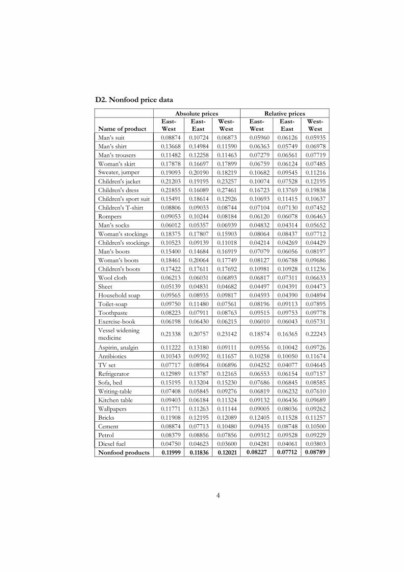
4
D2. Nonfood price data
Absolute prices Relative prices
Name of product East-West
East-East
West-West
East-West
East-East
West-West
Man’s suit 0.08874 0.10724 0.06873 0.05960 0.06126 0.05935 Man’s shirt 0.13668 0.14984 0.11590 0.06363 0.05749 0.06978 Man’s trousers 0.11482 0.12258 0.11463 0.07279 0.06561 0.07719 Woman’s skirt 0.17878 0.16697 0.17899 0.06759 0.06124 0.07485 Sweater, jumper 0.19093 0.20190 0.18219 0.10682 0.09545 0.11216 Children's jacket 0.21203 0.19195 0.23257 0.10074 0.07528 0.12195 Children's dress 0.21855 0.16089 0.27461 0.16723 0.13769 0.19838 Children's sport suit 0.15491 0.18614 0.12926 0.10693 0.11415 0.10637 Children's T-shirt 0.08806 0.09033 0.08744 0.07104 0.07130 0.07452 Rompers 0.09053 0.10244 0.08184 0.06120 0.06078 0.06463 Man’s socks 0.06012 0.05357 0.06939 0.04832 0.04314 0.05652 Woman’s stockings 0.18375 0.17807 0.15903 0.08064 0.08437 0.07712 Children's stockings 0.10523 0.09139 0.11018 0.04214 0.04269 0.04429 Man’s boots 0.15400 0.14684 0.16919 0.07079 0.06056 0.08197 Woman’s boots 0.18461 0.20064 0.17749 0.08127 0.06788 0.09686 Children's boots 0.17422 0.17611 0.17692 0.10981 0.10928 0.11236 Wool cloth 0.06213 0.06031 0.06893 0.06817 0.07311 0.06633 Sheet 0.05139 0.04831 0.04682 0.04497 0.04391 0.04473 Household soap 0.09565 0.08935 0.09817 0.04593 0.04390 0.04894 Toilet-soap 0.09750 0.11480 0.07561 0.08196 0.09113 0.07895 Toothpaste 0.08223 0.07911 0.08763 0.09515 0.09753 0.09778 Exercise-book 0.06198 0.06430 0.06215 0.06010 0.06043 0.05731 Vessel widening medicine 0.21338 0.20757 0.23142 0.18574 0.16365 0.22243
Aspirin, analgin 0.11222 0.13180 0.09111 0.09556 0.10042 0.09726 Antibiotics 0.10343 0.09392 0.11657 0.10258 0.10050 0.11674 TV set 0.07717 0.08964 0.06896 0.04252 0.04077 0.04645 Refrigerator 0.12989 0.13787 0.12165 0.06553 0.06154 0.07157 Sofa, bed 0.15195 0.13204 0.15230 0.07686 0.06845 0.08585 Writing-table 0.07408 0.05845 0.09276 0.06819 0.06232 0.07610 Kitchen table 0.09403 0.06184 0.11324 0.09132 0.06436 0.09689 Wallpapers 0.11771 0.11263 0.11144 0.09005 0.08036 0.09262 Bricks 0.11908 0.12195 0.12089 0.12405 0.11528 0.11257 Cement 0.08874 0.07713 0.10480 0.09435 0.08748 0.10500 Petrol 0.08379 0.08856 0.07856 0.09312 0.09528 0.09229 Diesel fuel 0.04750 0.04623 0.03600 0.04281 0.04061 0.03803 Nonfood products 0.11999 0.11836 0.12021 0.08227 0.07712 0.08789

4
D3. Services
Absolute prices Relative prices
Name of product East-West
East-East
West-West
East-West
East-East
West-West
Dry-cleaning 0.12409 0.07466 0.13441 0.12907 0.08106 0.11796Laundry and ironing 0.17940 0.14297 0.21899 0.05812 0.05015 0.06689Bath-house service 0.12504 0.12386 0.13341 0.11028 0.10972 0.11272Man's haircut 0.10997 0.10530 0.11697 0.04136 0.04481 0.03629Woman's haircut 0.05361 0.05732 0.04948 0.08324 0.06863 0.04673
Chemical hair curling 0.02117 0.02059 0.02171 0.10147 0.06802 0.04237Dental services 0.05160 0.05333 0.05170 0.11744 0.09213 0.11525Trousers sewing 0.06517 0.05872 0.07160 0.09890 0.05744 0.05727Dress sewing 0.05923 0.06019 0.05956 0.09286 0.05897 0.06706Man’s trousers repair service 0.10083 0.08258 0.12178 0.08957 0.08557 0.07804Shoes repair service 0.10272 0.10207 0.09385 0.03550 0.04312 0.02782Watch repair service 0.06171 0.04151 0.07806 0.07447 0.06557 0.05796Parking fee 0.06426 0.05326 0.07689 0.06254 0.04949 0.07226
Freight transportation 0.04155 0.02727 0.05390 0.13202 0.12701 0.14176Staying at the hotels 0.07688 0.07971 0.07518 0.12717 0.12350 0.11155Services of preschool institutions 0.17298 0.18006 0.16505 0.11573 0.11617 0.11694
Services of higher education institutions 0.06666 0.10425 0.01913 0.10123 0.10812 0.09847
Theatres 0.05166 0.04886 0.05007 0.12552 0.09903 0.11937Video tapes hire 0.10345 0.11593 0.09268 0.09760 0.08162 0.08565Photo for documents service 0.14974 0.11039 0.16308
0.04462 0.03902 0.05118
Art color photo service 0.03596 0.03560 0.03511 0.06914 0.06805 0.06413Services 0.08655 0.07993 0.08964 0.09085 0.07796 0.08037

4
APPENDIX E. DEVIATIONS FROM THE AVERAGE PRICE OF 4 BASKETS OF PRODUCTS ACROSS THE OBLASTS OF UKRAINE
Oblasts Basket of 29 food
products
Basket of 35 nonfood products
Basket of 21
services
Basket of all 85 products
Crimea 3.56% 6.23% 5.79% 5.82%Vinnytska -3.51% -3.71% -3.66% -3.63%Volynska -3.83% -2.46% -4.14% -4.12%Dnipropetrovska 6.95% 10.80% 12.88% 12.91%Donetska 8.47% 6.72% 8.08% 8.12%Zhytomyrska -2.23% -8.61% -9.41% -9.39%Zakarpatska -0.62% 5.25% 4.64% 4.68%Zaporizka 6.80% 0.08% 1.37% 1.40%Ivano-Frankivska -1.20% -4.55% -5.13% -5.10%Kyivska 4.95% 0.17% 0.59% 0.62%Kirovogradska -1.46% -0.81% -3.08% -3.05%Luganska 0.45% 6.38% 5.69% 5.72%Lvivska -1.63% 1.56% 3.00% 3.03%Mykolayivska 0.16% -2.93% -2.40% -2.37%Odeska 3.05% -0.43% 0.45% 0.48%Poltavska 1.32% -2.98% -2.44% -2.41%Rivnenska -5.29% 1.80% 1.10% 1.14%Sumska 2.09% -0.21% -2.16% -2.13%Ternopilska -8.98% -3.85% -4.01% -3.98%Kharkivska -2.89% -10.84% -9.56% -9.54%Khersonska 1.78% 2.16% 1.97% 2.00%Khmelnytska -5.96% -1.20% -1.67% -1.64%Cherkaska 0.96% -3.24% -0.32% -0.29%Chernivetska -3.53% 7.79% 7.44% 6.72%Chernigivska 0.59% -3.12% -5.01% -4.98%

4
APPENDIX E. CROSS-OBLAST COMPARISON OF THE WAGES DURING 1999-2004
Mean, UAH
Max, UAH
Min, UAH
Deviation from the average in Ukraine
Crimea 331.714 612.05 137.47 18.34% Vinnytska 253.973 531.56 105.2 -60.18% Volynska 240.322 498.89 98.08 -10.57% Dnipropetrovska 405.688 745.25 181.55 128.01% Donetska 425.724 816.27 188.18 15.51% Zhytomyrska 256.839 517.92 111.81 -130.73% Zakarpatska 277.997 553.82 104.81 16.38% Zaporizka 415.513 737.75 177.4 106.45% Ivano-Frankivska 300.1 598.32 111.78 -89.34% Kyivska 357.694 663.74 151.02 44.58% Kirovogradska 266.038 528.67 111.08 -70.95% Luganska 359.712 678.1 160.17 72.51% Lvivska 312.307 606.7 120.59 -36.70% Mykolayivska 353.336 633.01 142.84 31.76% Odeska 347.27 628.99 150.37 -4.70% Poltavska 334.187 641.78 139.68 -10.13% Rivnenska 288.705 614.57 113.28 -35.21% Sumska 289.835 543.67 123.01 0.87% Ternopilska 229.453 490.45 91.52 -46.74% Kharkivska 346.22 641.81 154.38 90.39% Khersonska 268.937 520.12 115.07 -59.82% Khmelnytska 247.442 500.8 108.03 -16.64% Cherkaska 268.68 546.98 119.6 16.44% Chernivetska 256.315 520.59 97.99 -9.57% Chernigivska 266.577 524.94 114.69 7.94%

4
APPENDIX G. LINGUISTIC DIFFERENCES ACROSS THE OBLASTS OF UKRAINE
Ukrainian-speaking
Russian-Speaking
Russian by origin
Crimea 10.0% 76.6% 58.3% Vinnytska 94.8% 4.7% 3.8% Volynska 97.3% 2.5% 2.4% Dnipropetrovska 67.0% 31.9% 17.6% Donetska 24.1% 74.9% 38.2% Zhytomyrska 93.0% 6.6% 5.0% Zakarpatska 81.0% 2.9% 2.5% Zaporizka 50.2% 48.2% 24.7% Ivano-Frankivska 97.8% 1.8% 1.8% Kyivska 92.3% 7.2% 13.1% Kirovogradska 88.9% 10.0% 7.5% Luganska 30.0% 68.8% 39.0% Lvivska 95.3% 3.8% 3.6% Mykolayivska 69.2% 29.3% 14.1% Odeska 46.3% 41.9% 20.7% Poltavska 90.0% 9.5% 7.2% Rivnenska 97.0% 2.7% 2.6% Sumska 83.3% 15.5% 9.4% Ternopilska 98.3% 1.2% 1.2% Kharkivska 53.8% 44.3% 25.6% Khersonska 73.2% 24.9% 14.1% Khmelnytska 95.2% 4.1% 3.6% Cherkaska 92.5% 6.7% 5.4% Chernivetska 75.6% 5.3% 4.1% Chernigivska 89.0% 10.3% 6.0%

4
APPENDIX H. STATA OUTPUT FOR SEPARATE OLS REGRESSIONS FOR EACH PRODUCT
H1. Standard deviation of )log()log(1,
1,
,
,itk
itj
itk
itj
PP
PP
−
−− used as a dependent variable
i) Food products
lndist border_polit border_hist common_border Dnipro R-sqr Wheaten bread 0.9793Rye bread -.0013684* .0018874** 0.9888Bun -.0035927* 0.9865Flour .0012801* -.0020624** 0.9935Rice .0014665** .0029199*** 0.9938Semolina 0.9945Buckwheat 0.9783Oats .0045567* 0.9808Beef .0016934* .0024042*** 0.9966Pork .0034325*** 0.9956Poultry .001796** .0015497* 0.9936Lard .0025072** 0.9961Smoked sausage .0119756*** -.0037665* -.0060477** .001634*** 0.9406Boiled sausage 0.9629Herring 0.9951Butter .0012451** -.0007703* 0.9946Sunflower oil -.0022232* 0.9935Milk .0020843*** 0.9965Sour cream, cream .0018376*** 0.9966Hard cheese .0012593** 0.9928Eggs .0077078*** .0029187*** 0.9942Sugar .0037753*** .0038604*** 0.9922Potato .016649*** .006699* 0.9878Cabbage .0217931*** -.0085771* 0.9926Onion .0100376** .0076904** 0.9920Beet .0113234** .0075082** 0.9907Carrot .0234727*** .0084863* -.0085106** 0.9898Vodka (alcohol) 0.9610Mineral water 0.9958
* significant at 10% level of significance ** significant at 5% level of significance *** significant at 1% level of significance

4
ii) Nonfood products
lndist border_polit border_hist common_border Dnipro R-sqr Man's suit .0060574* 0.9516 Man's shirt 0.9826 Man's trousers 0.9755 Woman's skirt 0.9959 Sweater, jumper 0.9742 Children's jacket .0032069*** 0.9951 Children's dress .0136164* 0.9234 Children's sport suit 0.9596 Children's T-shirt 0.9507 Rompers 0.9809 Man's socks 0.9385 Woman's stockings -.0034168** -.002739* 0.9940 Children's stockings -.0016312* 0.9769 Man's boots 0.9935 Woman's boots 0.9945 Children's boots .0062409* .006685* 0.9843 Wool cloth .0053712* 0.9633 Sheet .0033669* .0023059* 0.9670 Household soap .0016851** 0.9914 Toilet-soap 0.9462 Toothpaste .0123284** 0.9235 Exercise-book .0045838* 0.9593 Vessel widening medicine 0.9124 Aspirin, analgin 0.9003 Antibiotics -.0062018* 0.9500 TV set 0.9753 Refrigerator 0.9930 Sofa, bed 0.9928 Writing-table 0.9518 Kitchen table .0117448*** 0.9764 Wallpapers 0.9254 Bricks .0104764* .0165307* 0.9250 Cement 0.9388 Petrol 0.9176 Diesel fuel .0032206*** .0046494*** 0.9809
* significant at 10% level of significance ** significant at 5% level of significance *** significant at 1% level of significance

4
iii) Services
lndist border_polit border_hist common_border Dnipro R-sqr Dry-cleaning -.0165536** .0319492*** -.0210024** 0.9326 Laundry and ironing 0.9949 Bath-house service 0.9450 Man's haircut .0013326** 0.9918 Woman's haircut -.0063394* .0286513*** 0.9368 Chemical hair curling .0458037*** .0103751* 0.9207 Dental services .0178327* 0.8658 Trousers sewing .0122874*** .0355301*** .0112684* -.0071591* 0.9258 Dress sewing .0320362*** 0.8972 Shoes repair service 0.9922 Men's trousers repair service .0102677** -.0075205** 0.9474 Watch repair service .009685*** .0082786*** -.0078075** 0.9472 Parking fee 0.9055 Freight transportation 0.8496 Staying at the hotels -.0175705* -.0244894** -.0156352* 0.8994 Services of preschool institutions 0.9213 Services of higher education institutions 0.8801 Theatres .0189477*** 0.9198 Video tapes hire .0157478*** 0.8916 Photo for documents service 0.9781 Art color photo service 0.8748
* significant at 10% level of significance ** significant at 5% level of significance *** significant at 1% level of significance

4
H2. Standard deviation of )log(,
,itk
itj
PP
used as a dependent variable
i) Food products
lndist border_polit border_hist common_border Dnipro R-sqr Wheaten bread -.005208* .0065461* 0.9636 Rye bread -.0052367** 0.9627 Bun 0.9504 Flour 0.9775 Rice .0079797*** 0.9847 Semolina .0040885* 0.9794 Buckwheat .0052504*** 0.9799 Oats 0.9218 Beef .0163592*** .008625** -.0106664** .0101736* 0.9658 Pork .0078423** .0041066* 0.9786 Poultry .0062611** .0048325* 0.9752 Lard .0223701*** -.004916* .0200872*** 0.9826 Smoked sausage .0071018** 0.9434 Boiled sausage 0.9647 Herring .0047894** -.0027363* 0.9762 Butter .0064833*** .00585** 0.9653 Sunflower oil .0099176*** -.0067408* .0064314* 0.9753 Milk .0166679*** .0155948*** .0159622** 0.9579 Sour cream, cream .0106991** .0252961*** 0.9613 Hard cheese .006855** .0043769* .006211* 0.9771 Eggs .0133696*** .0047046*** .0060764*** 0.9865 Sugar .0108351*** .0044671*** -.0032857** 0.9862 Potato .0290099*** 0.9906 Cabbage .0602457*** .0104023** 0.9887 Onion .0226496*** .006586** 0.9908 Beet .0479771*** .0155027*** -.0130768** 0.9879 Carrot .0512824*** -.0138619*** 0.9906 Vodka (alcohol) .004396* -.0049936* 0.9692 Mineral water -.0108153* -.027032*** 0.9536
* significant at 10% level of significance ** significant at 5% level of significance *** significant at 1% level of significance

4
ii) Nonfood products
lndist border_polit border_hist common_border Dnipro R-sqr Man's suit 0.9393 Man's shirt 0.9428 Man's trousers .0111221* 0.9451 Woman's skirt .0317428*** -.0132472** 0.9654 Sweater, jumper -.0225651* 0.9361 Children's jacket 0.9652 Children's dress .018747* 0.9167 Children's sport suit -.0156253* 0.9305 Children's T-shirt .0084829* 0.9482 Rompers 0.9640 Man's socks 0.9057 Woman's stockings .0241809*** 0.9714 Children's stockings .0095138* 0.9615 Man's boots 0.9638 Woman's boots -.0093174* .0181867*** 0.9712 Children's boots 0.9594 Wool cloth 0.9608 Sheet 0.9322 Household soap .0082831* 0.9583 Toilet-soap 0.9437 Toothpaste 0.9588 Exercise-book .0077465* 0.9371 Vessel widening medicine 0.8722 Aspirin, analgin 0.9447 Antibiotics .0095883** 0.9537 TV set 0.9588 Refrigerator -.0102293** 0.9695 Sofa, bed .0118753** .0143359** 0.9597 Writing-table 0.9480 Kitchen table .0071971*** 0.9643 Wallpapers .0214254** .0071971 -.0140528* 0.9101 Bricks 0.9447 Cement 0.9561 Petrol 0.9496 Diesel fuel .0049615*** .0036706*** 0.9727
* significant at 10% level of significance ** significant at 5% level of significance *** significant at 1% level of significance
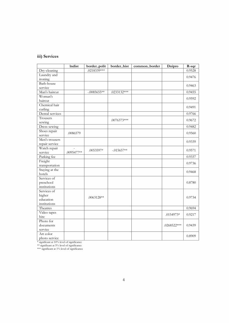
4
iii) Services
lndist border_polit border_hist common_border Dnipro R-sqr Dry-cleaning .0218339*** 0.9528 Laundry and ironing 0.9476
Bath-house service 0.9463
Man's haircut -.0085655** .0233132*** 0.9455 Woman's haircut 0.9592
Chemical hair curling 0.9491
Dental services 0.9766 Trousers sewing .0076373*** 0.9672
Dress sewing 0.9482 Shoes repair service .0086579 0.9560
Men's trousers repair service 0.9339
Watch repair service
-.0095477** .0053597* -.015657** 0.9571
Parking fee 0.9337 Freight transportation 0.9736
Staying at the hotels 0.9468
Services of preschool institutions
0.8780
Services of higher education institutions
.0063128** 0.9734
Theatres 0.9694 Video tapes hire .0154973* 0.9217
Photo for documents service
.0268522*** 0.9439
Art color photo service 0.8909
* significant at 10% level of significance ** significant at 5% level of significance *** significant at 1% level of significance