EXAMINING ASPECTS OF COPPER AND BRASS CORROSION IN DRINKING WATER

Nestor Agustin Murray-Ramos

Thesis submitted to the Faculty of the Virginia Polytechnic Institute and State University

in partial fulfillment of the requirements for the degree of

Master of Science in

Environmental Engineering

Dr. Marc Edwards, Chair Dr. Andrea Dietrich Dr. G.V. Loganathan

November 3, 2006 Blacksburg, Virginia USA

Keywords: Corrosion, Copper, Brass, Pitting, Chlorine, Chloramines, Aluminum, Flow, Chloride:Sulfate, Phosphate, NOM, Lead, ANSI/NSF 61 – Section 6

ABSTRACT

Examining Aspects of Copper and Brass Corrosion in Drinking Water

Nestor Agustin Murray-Ramos

As the water industry complies with the new arsenic standard and new treatments are installed, unintended consequences might be expected in relation to corrosion control when sulfate/chloride ratio, pH, phosphate, iron, aluminum, bicarbonate and organic matter levels are altered. In some cases, these changes will be beneficial and in other detrimental. This research project is the first to systematically evaluate the effect of some key changes in the chemistry of the treated water in relation to copper and brass corrosion control. A 1.25 year pipe rig experiment was executed to anticipate effects of arsenic treatment on copper pinholes in 10 representative waters. The control water will mimic a synthesized version of Potomac River that is extremely aggressive to copper. Consistent with prior research that pitting is driven by free chlorine in this water and inhibited by phosphate, substitution of chloramine for chlorine or dosing of phosphate completely eliminated deep pits on tubes for the duration of the experiment. Chlorine caused serious pitting if NOM was less than 0.3 mg/L over a range of Cl:SO4 ratio’s. Pitting seemed to occur under deposits of iron or aluminum on the copper surface, and if anything, an equimolar amount of iron caused worse pitting than aluminum. Amendment of the aggressive water with 3 mg/L NOM eliminated growth of deep pits (> 0.05 mm). While brass pipes (containing 0.09% lead, 63% copper and 36% zinc) was attacked non-uniformally by an aggressive water at high pH and with high Cl2 content, no significant pitting occurred at any condition tested, even though pitting did occur for copper exposed to the exact same water. The implication is that zinc in the alloy may help to prevent non-uniform attack on copper and copper alloys.

The ban on lead-containing plumbing materials in the Safe Drinking Water Act (1986) and the EPA Lead and Copper Rule (1991) have successfully reduced lead contamination of potable water supplies. This part of the work carefully re-examined the lead contamination concern from the standpoint of existing performance standards for brass. The ANSI/NSF 61, Section 8 standard is relied on to protect the public from in-line brass plumbing products that might leach excessive levels of lead to potable water. Experiments were conducted to look at the practical strictness of these test-standards. In-depth study of the standard revealed serious flaws due from the use of a phosphate buffer and a failure to control carbonate dissolution from the atmosphere in the test waters. In order to help prevent undesirable outcomes in the future, standard’s improvements are needed to assurance that brass devices passing this test are safe.

iii

ACKNOWLEDGEMENTS

Thanks to my advisor and mentor, Marc Edwards, for his guidance, patience and endless positive encouragement, and for making this thesis and my valuable graduate school

experience possible.

Marc, Gracias for never giving up on me.

Thanks also to the Edwards Research Group, Faculty and Laboratory Support for their help and encouragement.

Thanks also to the American Water Works Association Research Foundation and the Copper Development Association for their generous funding.

Finally, thanks to my devoted family and friends, whose support has made all of my accomplishments possible.

This thesis is dedicated to Nestor Murray-Irrizarry and Carmen Iris Ramos…

iv

ATTRIBUTION The three chapters of this thesis are presented as separate manuscripts according to specifications of Virginia Tech’s journal article format. Chapter 1 and 2 were produced via collaboration between Nestor Murray (graduate student) and Marc Edwards (graduate advisor). As is typical for an M.S. thesis, Edwards provided the topic of study, direction during research procedures and grammatical corrections. Nestor Murray did work typical of a graduate research assistant on the project. Chapter 1 and 2 is an investigation of the pitting propensity of copper and brass corrosion, respectively. Chapter 3 was produced via collaboration between Nestor Murray (graduate student), Abhijeet Dudi (graduate student), Marc Edwards (graduate advisor), and Michael Schock (Environmental Protection Agency researcher). Murray did the original experimental setup in the work and maintained the rigs for the first 3 months. Edwards and Schock provided intellectual input typical of graduate advisors and the paper was part of Dudi’s thesis. Chapter 3 critically evaluates and examines the practical rigor of the NSF 61 section 8 testing procedure that is relied on to protect public health. The results highlight the need for an improved standard to certify lead bearing brass devices. The author of this thesis was fourth author on this publication. This study was presented at the AWWA Annual Conference in June of 2006 and part of it appears in the proceedings of that conference. A refined version of this chapter was published in Journal American Water Works Association (JAWWA).

v

TABLE OF CONTENTS

ABSTRACT ii

ACKNOWLEDGEMENTS iii

AUTHOR'S PREFACE iv

TABLE OF CONTENTS v

LIST OF TABLES vii

LIST OF FIGURES viii

CHAPTER 1: EFFECT OF ION EXCHANGE AND OTHER TREATMENTS ON NON-UNIFORM CORROSION OF COPPER 1

INTRODUCTION………………………………………………………………………….1

EXPERIMENTAL MATERIALS AND METHODS……………………………………..3

Aluminum Dosing 5 Chloramine Dosing 6 NOM Dosing 6

Electrochemical Measurements 6

Water chemistry measurements 6

Visual Observations of Pipes 6 Analysis of Pipes 7

Experimental Timeline 7

RESULTS AND DISCUSSION ......................................................................................... 8

Visual Analysis of Copper Surface 9 Characterization of Pitting Propensity 15 Pit Location and Density 17 Weight Loss and Leaching 21 Scaling and Scale Identity 20 Kinetics of Chlorine Decay 28 Electrochemistry of Pitting 30

DISCUSSION ................................................................................................................... 37

CONCLUSIONS............................................................................................................... 38

REFERENCES.................................................................................................................. 40

vi

CHAPTER 2: EFFECT OF ION EXCHANGE AND OTHER TREATMENTS ON NON-UNIFORM CORROSION OF BRASS 41

ABSTRACT………………………………………………………………………………41 INTRODUCTION…………………………………………………………………..……41 Experimental Methods and Materials 41

RESULTS AND DISCUSSION………………………………………………………….43

Visual Analysis of Copper Surface 43 Weight Loss and Leaching 46 Scaling and Scale Identity 48 Electrochemistry of Brass Corrosion 52

CONCLUSION………………………………………………………………………...…57

CHAPTER 3: LEAD LEACHING FROM IN-LINE BRASS DEVICES: A CRITICAL EVALUATION OF THE EXISTING STANDARD 58

ABSTRACT...................................................................................................................... 58

INTRODUCTION............................................................................................................. 58

MATERIALS AND METHODS...................................................................................... 66

RESULTS AND DISCUSSION ....................................................................................... 68

Consideration of Test Water Chemistry 68 Effect of Phosphate on Lead Leaching Propensity of the NSF pH 5 Water 72 Effect of aeration on Lead Leaching Propensity of the NSF pH 10 Water 78 Considering the Overall Rigor of the Test 80 Retrospective Evaluation and Recommendations 83

CONCLUSIONS………………………………………………………………………….87

ACKNOWLEDGEMENTS………………………………………………………………87

REFERENCES……………………………………………………………………………89

vii

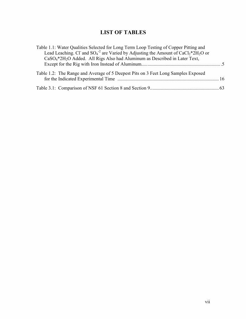
LIST OF TABLES

Table 1.1: Water Qualities Selected for Long Term Loop Testing of Copper Pitting and Lead Leaching. Cl- and SO4

-2 are Varied by Adjusting the Amount of CaCl2*2H2O or CaSO4*2H2O Added. All Rigs Also had Aluminum as Described in Later Text, Except for the Rig with Iron Instead of Aluminum................................................................. .5

Table 1.2: The Range and Average of 5 Deepest Pits on 3 Feet Long Samples Exposed for the Indicated Experimental Time .................................................................................... 16

Table 3.1: Comparison of NSF 61 Section 8 and Section 9......................................................... 63

viii

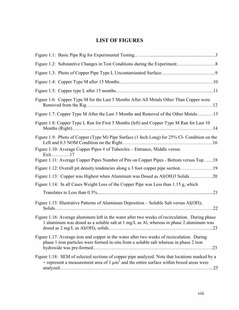
LIST OF FIGURES

Figure 1.1: Basic Pipe Rig for Experimental Testing.………........................................................3

Figure 1.2: Substantive Changes in Test Conditions during the Experiment…………………….8

Figure 1.3: Photo of Copper Pipe Type L Uncontaminated Surface……………………………..9

Figure 1.4: Copper Type M after 15 Months……………………………………………………10

Figure 1.5: Copper type L after 15 months……………………………………………………...11

Figure 1.6: Copper Type M for the Last 5 Months After All Metals Other Than Copper were Removed from the Rig………………………………………………………………………12

Figure 1.7: Copper Type M After the Last 3 Months and Removal of the Other Metals.….……13

Figure 1.8: Copper Type L Ran for First 5 Months (left) and Copper Type M Ran for Last 10 Months (Right)………………………………………………………………………………14

Figure 1.9: Photo of Copper (Type M) Pipe Surface (1 Inch Long) for 25% Cl- Condition on the Left and 0.3 NOM Condition on the Right………………………………………………….16

Figure 1.10: Average Copper Pipes # of Tubercles – Entrance, Middle versus Exit…………17

Figure 1.11: Average Copper Pipes Number of Pits on Copper Pipes - Bottom versus Top……18

Figure 1.12: Overall pit density tendencies along a 3 foot copper pipe section…………………19

Figure 1.13: Copper was Highest when Aluminum was Dosed as Al(OH)3 Solids……………20

Figure 1.14: In all Cases Weight Loss of the Copper Pipe was Less than 1.15 g, which

Translates to Less than 0.3%...................................................................................................21

Figure 1.15: Illustrative Patterns of Aluminum Deposition – Soluble Salt versus Al(OH)3 Solids………………………………………………………………………………………...22

Figure 1.16: Average aluminum left in the water after two weeks of recirculation. During phase 1 aluminum was dosed as a soluble salt at 1 mg/L as Al, whereas in phase 2 aluminum was dosed as 2 mg/L as Al(OH)3 solids.………………………………………………………....23

Figure 1.17: Average iron and copper in the water after two weeks of recirculation. During phase 1 iron particles were formed in-situ from a soluble salt whereas in phase 2 iron hydroxide was pre-formed.………………………………………………………………….23

Figure 1.18: SEM of selected sections of copper pipe analyzed. Note that locations marked by a + represent a measurement area of 1 µm2 and the entire surface within boxed areas were analyzed……………………………………………………………………………………...25

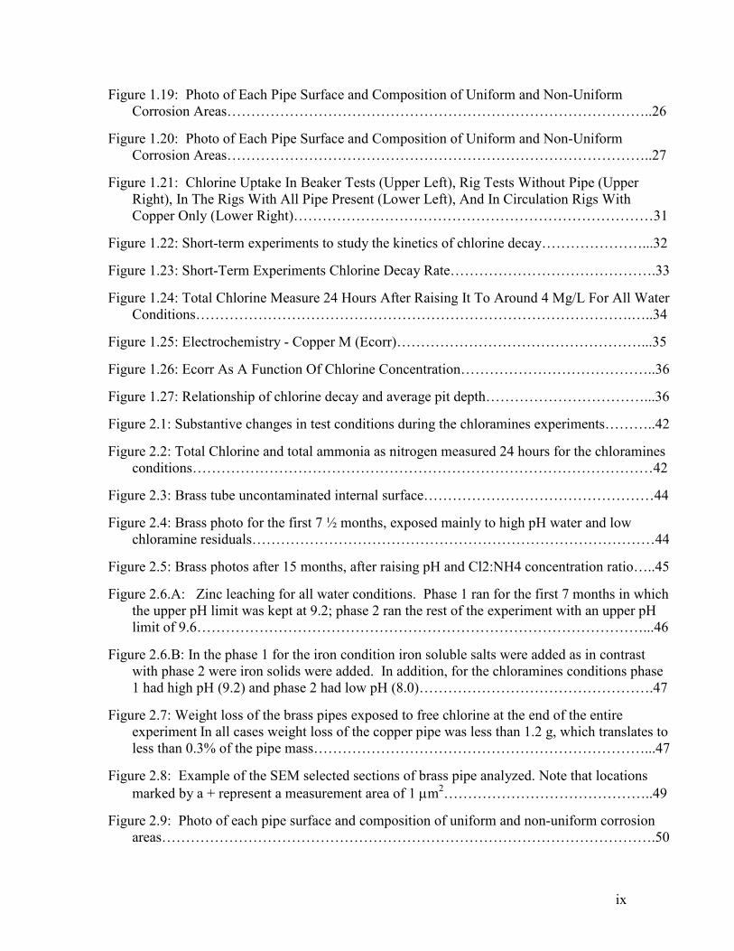
ix

Figure 1.19: Photo of Each Pipe Surface and Composition of Uniform and Non-Uniform Corrosion Areas……………………………………………………………………………..26

Figure 1.20: Photo of Each Pipe Surface and Composition of Uniform and Non-Uniform Corrosion Areas……………………………………………………………………………..27

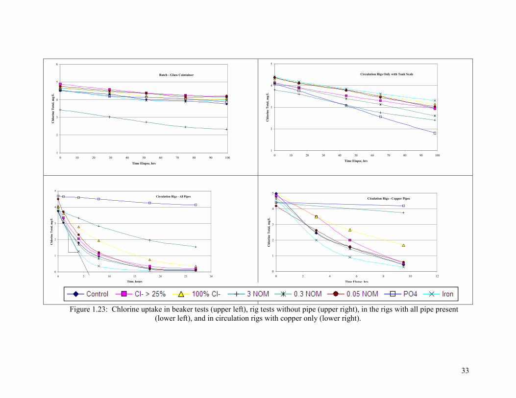
Figure 1.21: Chlorine Uptake In Beaker Tests (Upper Left), Rig Tests Without Pipe (Upper Right), In The Rigs With All Pipe Present (Lower Left), And In Circulation Rigs With Copper Only (Lower Right)…………………………………………………………………31

Figure 1.22: Short-term experiments to study the kinetics of chlorine decay…………………...32

Figure 1.23: Short-Term Experiments Chlorine Decay Rate…………………………………….33

Figure 1.24: Total Chlorine Measure 24 Hours After Raising It To Around 4 Mg/L For All Water Conditions……………………………………………………………………………….…..34

Figure 1.25: Electrochemistry - Copper M (Ecorr)……………………………………………...35

Figure 1.26: Ecorr As A Function Of Chlorine Concentration…………………………………..36

Figure 1.27: Relationship of chlorine decay and average pit depth……………………………...36

Figure 2.1: Substantive changes in test conditions during the chloramines experiments………..42

Figure 2.2: Total Chlorine and total ammonia as nitrogen measured 24 hours for the chloramines conditions……………………………………………………………………………………42

Figure 2.3: Brass tube uncontaminated internal surface…………………………………………44

Figure 2.4: Brass photo for the first 7 ½ months, exposed mainly to high pH water and low chloramine residuals…………………………………………………………………………44

Figure 2.5: Brass photos after 15 months, after raising pH and Cl2:NH4 concentration ratio…..45

Figure 2.6.A: Zinc leaching for all water conditions. Phase 1 ran for the first 7 months in which the upper pH limit was kept at 9.2; phase 2 ran the rest of the experiment with an upper pH limit of 9.6…………………………………………………………………………………...46

Figure 2.6.B: In the phase 1 for the iron condition iron soluble salts were added as in contrast with phase 2 were iron solids were added. In addition, for the chloramines conditions phase 1 had high pH (9.2) and phase 2 had low pH (8.0)………………………………………….47

Figure 2.7: Weight loss of the brass pipes exposed to free chlorine at the end of the entire experiment In all cases weight loss of the copper pipe was less than 1.2 g, which translates to less than 0.3% of the pipe mass……………………………………………………………...47

Figure 2.8: Example of the SEM selected sections of brass pipe analyzed. Note that locations marked by a + represent a measurement area of 1 µm2……………………………………..49

Figure 2.9: Photo of each pipe surface and composition of uniform and non-uniform corrosion areas………………………………………………………………………………………….50

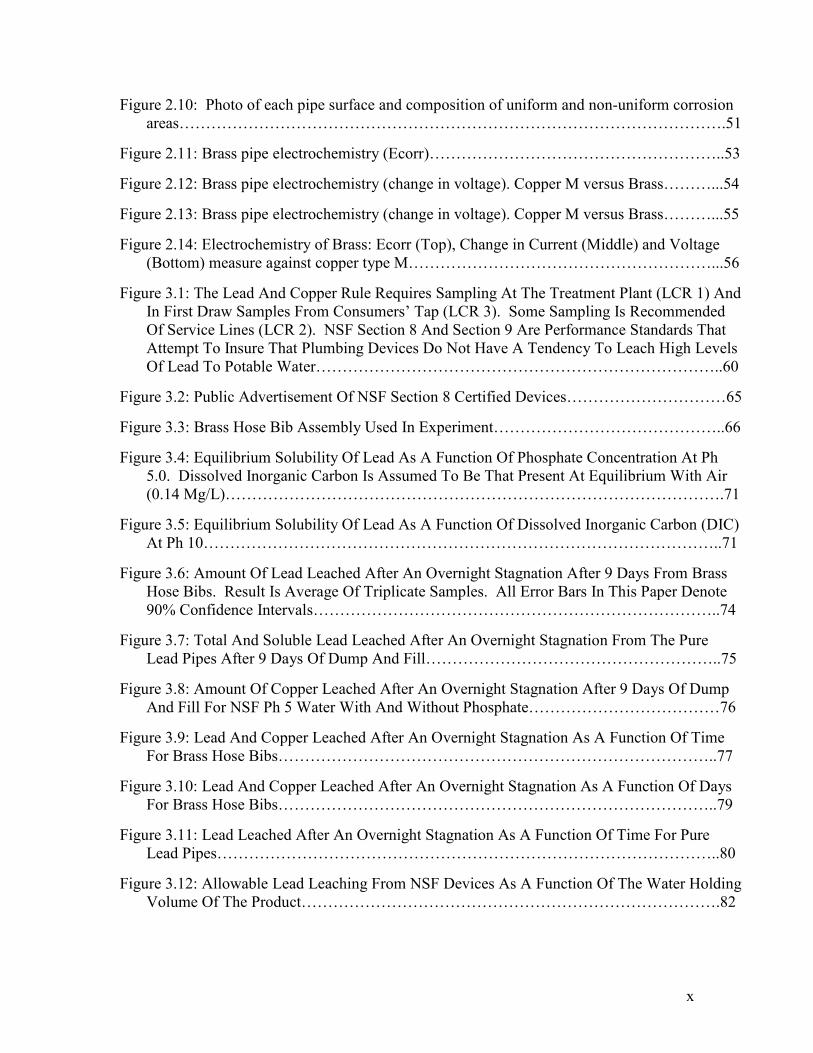
x

Figure 2.10: Photo of each pipe surface and composition of uniform and non-uniform corrosion areas………………………………………………………………………………………….51

Figure 2.11: Brass pipe electrochemistry (Ecorr)………………………………………………..53

Figure 2.12: Brass pipe electrochemistry (change in voltage). Copper M versus Brass………...54

Figure 2.13: Brass pipe electrochemistry (change in voltage). Copper M versus Brass………...55

Figure 2.14: Electrochemistry of Brass: Ecorr (Top), Change in Current (Middle) and Voltage (Bottom) measure against copper type M…………………………………………………...56

Figure 3.1: The Lead And Copper Rule Requires Sampling At The Treatment Plant (LCR 1) And In First Draw Samples From Consumers’ Tap (LCR 3). Some Sampling Is Recommended Of Service Lines (LCR 2). NSF Section 8 And Section 9 Are Performance Standards That Attempt To Insure That Plumbing Devices Do Not Have A Tendency To Leach High Levels Of Lead To Potable Water…………………………………………………………………..60

Figure 3.2: Public Advertisement Of NSF Section 8 Certified Devices…………………………65

Figure 3.3: Brass Hose Bib Assembly Used In Experiment……………………………………..66

Figure 3.4: Equilibrium Solubility Of Lead As A Function Of Phosphate Concentration At Ph 5.0. Dissolved Inorganic Carbon Is Assumed To Be That Present At Equilibrium With Air (0.14 Mg/L)………………………………………………………………………………….71

Figure 3.5: Equilibrium Solubility Of Lead As A Function Of Dissolved Inorganic Carbon (DIC) At Ph 10……………………………………………………………………………………..71

Figure 3.6: Amount Of Lead Leached After An Overnight Stagnation After 9 Days From Brass Hose Bibs. Result Is Average Of Triplicate Samples. All Error Bars In This Paper Denote 90% Confidence Intervals…………………………………………………………………..74

Figure 3.7: Total And Soluble Lead Leached After An Overnight Stagnation From The Pure Lead Pipes After 9 Days Of Dump And Fill………………………………………………..75

Figure 3.8: Amount Of Copper Leached After An Overnight Stagnation After 9 Days Of Dump And Fill For NSF Ph 5 Water With And Without Phosphate………………………………76

Figure 3.9: Lead And Copper Leached After An Overnight Stagnation As A Function Of Time For Brass Hose Bibs………………………………………………………………………..77

Figure 3.10: Lead And Copper Leached After An Overnight Stagnation As A Function Of Days For Brass Hose Bibs………………………………………………………………………..79

Figure 3.11: Lead Leached After An Overnight Stagnation As A Function Of Time For Pure Lead Pipes…………………………………………………………………………………..80

Figure 3.12: Allowable Lead Leaching From NSF Devices As A Function Of The Water Holding Volume Of The Product…………………………………………………………………….82

1

CHAPTER 1: EFFECT OF ION EXCHANGE AND OTHER

TREATMENTS ON NON-UNIFORM CORROSION OF COPPER

Nestor Murray and Marc Edwards

Department of Civil and Environmental Engineering Virginia Polytechnic Institute and State University

Blacksburg, VA 24061 USA

ABSTRACT. The pitting propensity of copper in a range of waters that might be produced via arsenic treatment examined in a 15 month experiment. In this water at high pH in which pitting is believed to be driven by free chlorine, important qualitative trends were obtained in relation to pitting propensity. Chloramine did not cause significant pitting either alone or in combination with orthophosphate. Chlorine caused serious pitting if NOM was less than 0.3 mg/L over a range of Cl:SO4 ratio’s. Pitting seemed to occur under deposits of iron or aluminum on the copper surface, and if anything, an equimolar amount of iron caused worse pitting than aluminum. Amendment of the aggressive water with 3 mg/L NOM or 1 mg/L orthophosphate eliminated growth of deep pits (> 0.05 mm).

INTRODUCTION

Copper is the dominant tube used in homes and buildings, and while it has recently lost

market share to PEX and PVC, as of 2001 it still accounted for most new tube

installations as recently as 2001 (Marshultz, 2001). The net present replacement value of

plumbing tube installed in U.S. buildings and service lines is on the order of 1 trillion

dollars (Edwards, 2004a), which exceeds the net present replacement value of large pipe

used in potable water distribution by a considerable margin (Brongers, 2002 ). This

valuable assest is therefore deserving of protection.

It has long been understood that certain water treatments can increase the likelihood of

pinhole leaks in copper tube (Edwards et al., 1994), and it is believed that such treatments

have contributed to epidemic levels of pinhole leaks in a few areas of the country

(Edwards et al., 2004b; Rushing et al., 2004). One outbreak at a large utility in Maryland

ultimately caused leaks in 20-50% of the homes (Edwards et al., 2004b). In 2004, it was

unambiguously proven that water alone could eat a pinhole leak in copper tube, and that

imperfections in the tube or poor installation and other factors are not required (Marshall,

2

2004a). This does not mean that these other factors do not sometimes exert a significant

influence or even control pitting.

The effective changes to treatment that are believed to have caused outbreaks of leaks

include removal of organic matter, higher pH, higher chlorine residuals in water, and

increased concentration of aluminum residuals (Edwards, et al., 1994; Rushing et al.,

2004). It is suspected that a switch to chloramine can also sometimes contribute to the

problem. Prompted by a few serious outbreaks of pitting, several research projects are

underway to assess the frequency of pinhole leaks and to develop methods of monitoring

for aggressive water.

Although the arsenic regulation is still in its infancy and pinholes might take years to eat

through a pipe wall in some cases, there have already been two reported cases in which it

was believed that new arsenic treatments caused pinhole leaks in copper. The first

reportedly occurred in a medical facility fed water from anion exchange treatments. A

building riddled with copper leaks had to be completely replumbed at a cost of tens of

thousands of dollars. The second instance involved point of use installation of activated

alumina, which is believed to have caused leaks in both brass and copper plumbing

materials under a deposit of aluminum on the tube surface. In the latter case, we

speculate that higher aluminum residuals in the water from the activated alumina likely

contributed to the problem, along with higher pHs and moderate free chlorine (e.g.,

Rushing et al., 2004). In the former case with anion exchange the altered levels of Cl-,

SO4-2, bicarbonate, pH and natural organic matter are likely contributors. It is currently

believed that there are many forms of pitting, some of which occur at low pH and some

of which occur at high pH (Edwards et al., 1994), so effects of treatment changes are

expected to vary from water to water.

Given the devastating economic consequences of pinhole leaks, which can cost over

hundred thousand dollars per building after considering water damages, replumbing,

insurance implications and mold growth (Edwards et al, 2004b), it was deemed desireable

to develop some preliminary information on some impacts of arsenic treatment in longer

3

term experiments. This work therefore examines effects of modifications to water

chemistry that might occur from arsenic treatments on non-uniform copper corrosion

tendencies.

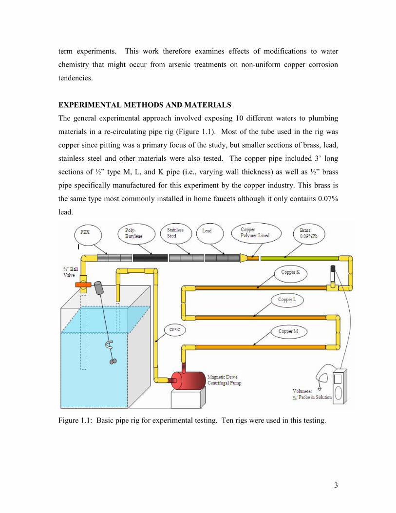
EXPERIMENTAL METHODS AND MATERIALS

The general experimental approach involved exposing 10 different waters to plumbing

materials in a re-circulating pipe rig (Figure 1.1). Most of the tube used in the rig was

copper since pitting was a primary focus of the study, but smaller sections of brass, lead,

stainless steel and other materials were also tested. The copper pipe included 3’ long

sections of ½” type M, L, and K pipe (i.e., varying wall thickness) as well as ½” brass

pipe specifically manufactured for this experiment by the copper industry. This brass is

the same type most commonly installed in home faucets although it only contains 0.07%

lead.

Figure 1.1: Basic pipe rig for experimental testing. Ten rigs were used in this testing.

4

The 10 waters were derived from a recipe described by Marshall (2004b) which had been

proven to cause fully penetrating pinholes (8 leaks per foot) in Type M copper tube

within 11 months. The control water for the current work had about 33% higher meq/L

of SO4-2 and 33% lower meq/L Cl- than the Marshall water, and was constituted by

adding 6.26 g CaCl2*2H2O, 4.89 g of CaSO4*2H2O and 10.75 g of NaHCO3 to 50 gallons

of distilled water. The pH was raised to 9.2 using 10 mL of 5 M NaOH).

The other nine waters are modifications of the control and were designed to represent a

wide range of waters that might be produced by anion exchange arsenic treatment (Table

1). To represent partial anion exchange treatment of the control water, the meq/L Cl- was

increased 25% and the meq/L sulfate was decreased 25%, thereby producing a water

virtually identical to the Marshall recipe that had been proven to cause severe pitting. To

represent complete anion exchange treatment of the control water, all the meq/L SO4-2

was replaced with Cl-. In other words, the sum of the Cl- and SO4-2 remain constant in

each test, as would occur during anion exchange. All test waters also had 0.86 meq/L of

Ca+2 and alkalinity of 34 mg/L as CaCO3. The target pH was 9.2 and chlorine was dosed

to 4 mg/L using reagent grade bleach. Aluminum was also added to the water as a

catalyst for initiation of non-uniform corrosion as specified in initial experiments.

The tests in which different levels of NOM were added to the control were designed to

simulate a range of NOM concentrations that might occur after activated alumina (AA),

ion exchange (IX) or granular ferric hydroxide (GFH) treatment since these treatments

can remove NOM. Other tests were conducted with an iron residual in the water instead

of an aluminum residual, to compare different possible effects of iron and aluminum

deposits on non-uniform copper corrosion. Finally, still other tests were conducted with

4 mg/L chloramine instead of chlorine, chloramine plus phosphate, and chlorine plus

phosphate (Table 1.1).

5

Table 1.1: Water qualities selected for long term loop testing of copper pitting and lead

leaching. Cl- and SO4-2 are varied by adjusting the amount of CaCl2*2H2O or

CaSO4*2H2O added. All rigs also had aluminum as described in later text, except for the

rig with iron instead of aluminum.

Descriptor of

water to be used

throughout the

report

SO4-2

Meq

Cl-

meq

NOM

mg/L

as C

Comments on practical reason for

modification

Control 0.30 0.56 0 Water known to cause pitting Higher Cl- and Lower SO4

-2 0.16 0.70 0 Partial anion exchange treatment*

All Cl- 0 0.86 0 Complete anion exchange treatment 0.05 NOM 0.30 0.56 0.05 Removal of most NOM by As

treatments 0.3 NOM 0.30 0.56 0.3 Removal of some NOM by As

treatments 3 NOM 0.30 0.56 3 Water with high NOM for comparison PO4 0.30 0.56 0 Determine if 1 mg/L PO4-P can prevent

lead leaching or pitting relative to control

Iron 0.30 0.56 0 Dosing of 2 mg/L iron (and no aluminum) simulates effect of GFH fines on pitting and lead leaching

NH4 0.30 0.56 0 Monochloramine formed by adding ammonia

NH4 & PO4 0.30 0.56 0 Determine effects of dosing phosphate and chloramine on lead leaching and pitting.

*This water is virtually identical to that used by Marshall et al., 2004.

Aluminum Dosing. After changing the water every other week, aluminum was added to

a final concentration of either 2 mg/L (as Al) using freshly prepared Al(OH)3 solids or 1

mg/L aluminum salts as specified. When the aluminum was dosed in a “soluble” form,

AlCl3 was added directly to the water and stirred until it dissolved. The aluminum

probably precipitated rapidly in the water as Al(OH)3 or similar solids. When the

aluminum was added as a solid, an Al(OH)3 (s) stock solution was created by raising the

pH of a 1,500 mg/L AlCl3 solution to pH 9.0 using NaOH, followed by repeated

rinsing/decanting of water over settled solids until the conductivity of the solution

6

dropped below that of the experimental water. After rapid mixing aluminum solids were

dosed from this stock solution.

Chloramine Dosing. In the case of the two rigs with chloramine as a disinfectant,

ammonia hydroxide (1M NH3OH) was added first, followed by addition of diluted

chlorine while stirring rapidly. A dose of 4:1 Cl2/NH3-N was achieved as confirmed via

total chlorine and total ammonia measurements.

NOM Dosing. Prior to water changes, natural organic matter (NOM) was pre-

chlorinated as would often occur in water treatment. It was determined that a dose of 30

mL of reagent grade NaOCl added to 38 mL NOM concentrated stock solution, diluted to

a total volume of 200 mLs gave a residual of about 1 mg/L Cl2 after 24 hours. This

meant that the vast majority of the chlorine demand of the NOM stock solution was met

through pre-chlorination, and that the NOM was similar to that occurring in many

distribution systems since it was pre-chlorinated. The pre-chlorinated NOM was then

filtered through a 5 µm pore size filter before dilution as needed for experiments.

Electrochemical Measurements. A variety of electrochemical measurements were

made for the copper pipes. The corrosion potential (Ecorr) was obtained using a

multimeter and a AgCl double junction reference electrode. These values are reported in

millivolts (mV) versus AgCl. The KCl reference electrodes were checked and

maintained regularly to ensure accuracy.

Water chemistry measurements. Dissolved and total metal concentrations in the water

were tracked during the experiments using ion exchange (IC), inductively coupled plasma

mass spectroscopy (ICP-MS) and TOC sampling before and after each water change.

Visual Observations of Pipes. Originally 3’ long sections of ½” type M, L, and K pipe

were included in the rig (Figure 1.3). The copper type M and L pipes were exposed for

the whole experiment, whereas the K pipe was taken out at 12 months to check for depth

7

of pits and SEM analysis. Other very small sections (e.g., up to 3") were removed from

the rig during the experiment.

Analysis of Pipes. After the experiment pipe samples were dried, weighed and then cut

lengthwise to preserve separate top and bottom sections for inspection of pit density and

pit depth. Overall weight loss was determined by measuring the pipe segment weight

before the experiment, the pipe segment weight after the experiment, and the amount of

scale removed from the pipe after cleaning with a felt-tipped Dremel tool (i.e., Weight

Loss = Initial Pipe Weight – Scale – Final Weight). The extent of pitting was determined

by visual counting of pits, determining pit depth (i.e., Pit Depth = initial wall thickness -

final wall thickness at pits), and using a 0-25 mm caliper to measure wall thickness with

an accuracy of 0.01 mm. Scanning electron microscopy and ESCA were using for

detailed analysis of the surfaces.

Experimental Timeline. During the first few months of the experiment, it became clear

that the electrochemical behavior of the rig was not consistent with that which had been

observed by Marshall, even for the water that had virtually identical initial chemistry.

Specifically, very high levels of Ecorr (> 1 V versus AgCl reference electrode) believed to

be consistent with rapid pitting that were observed in the Marshall test were not observed

in this experiment. Since the primary goal of the experiments was to replicate copper

pitting and to judge relative effects of water chemistry changes by comparison, several

attempts were made to try and determine the factors that might be preventing very rapid

pitting in the current work.

A list of potential differences between the current rig relative to that of Marshall was

compiled. Differences included 1) presence of brass and other metals in the rig, 2) initial

dosing of aluminum from soluble salts instead of Al(OH)3 particles, 3) use of internal

velocity of 8 feet per second flow rate instead of 2 feet per second, 3) use of ½” diameter

pipe instead of ¾” pipe, and 4) free Cl2 restored to 4 mg/L once per day in the current

work versus constant 4 mg/L achieved via continuous dosing.

8

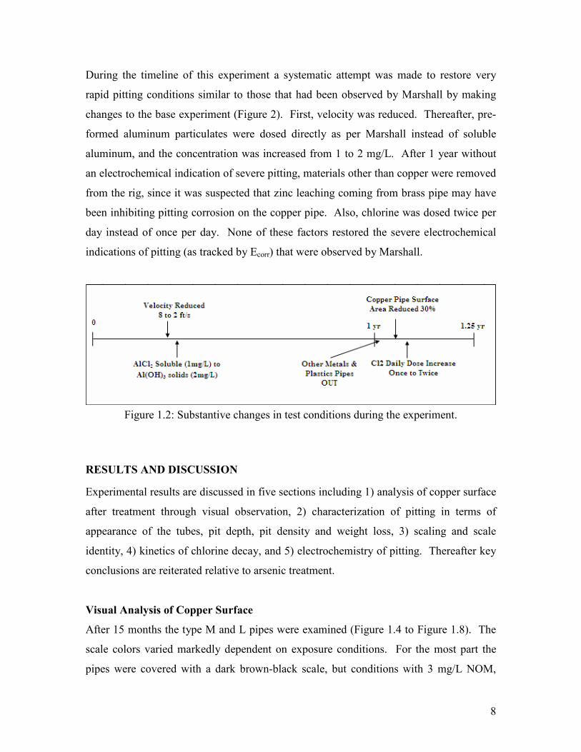
During the timeline of this experiment a systematic attempt was made to restore very

rapid pitting conditions similar to those that had been observed by Marshall by making

changes to the base experiment (Figure 2). First, velocity was reduced. Thereafter, pre-

formed aluminum particulates were dosed directly as per Marshall instead of soluble

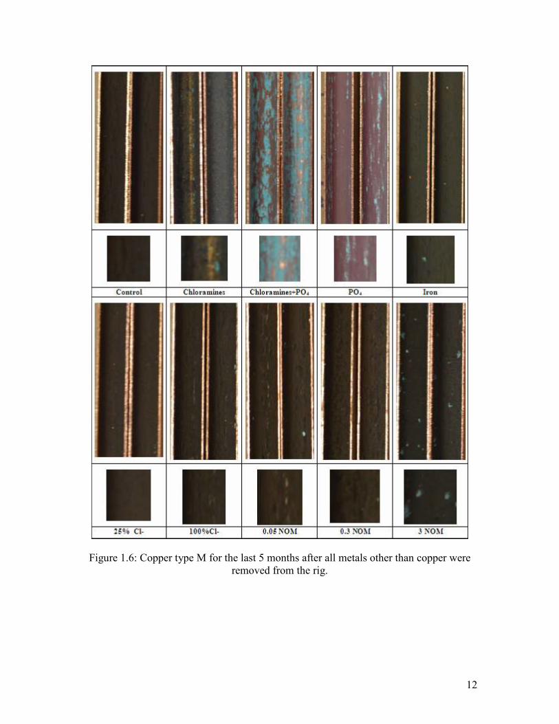
aluminum, and the concentration was increased from 1 to 2 mg/L. After 1 year without

an electrochemical indication of severe pitting, materials other than copper were removed

from the rig, since it was suspected that zinc leaching coming from brass pipe may have

been inhibiting pitting corrosion on the copper pipe. Also, chlorine was dosed twice per

day instead of once per day. None of these factors restored the severe electrochemical

indications of pitting (as tracked by Ecorr) that were observed by Marshall.

Figure 1.2: Substantive changes in test conditions during the experiment.

RESULTS AND DISCUSSION

Experimental results are discussed in five sections including 1) analysis of copper surface

after treatment through visual observation, 2) characterization of pitting in terms of

appearance of the tubes, pit depth, pit density and weight loss, 3) scaling and scale

identity, 4) kinetics of chlorine decay, and 5) electrochemistry of pitting. Thereafter key

conclusions are reiterated relative to arsenic treatment.

Visual Analysis of Copper Surface

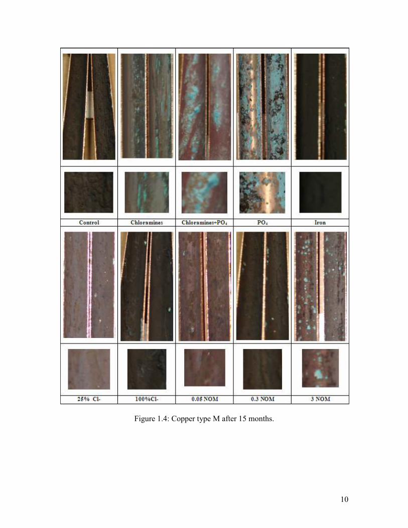
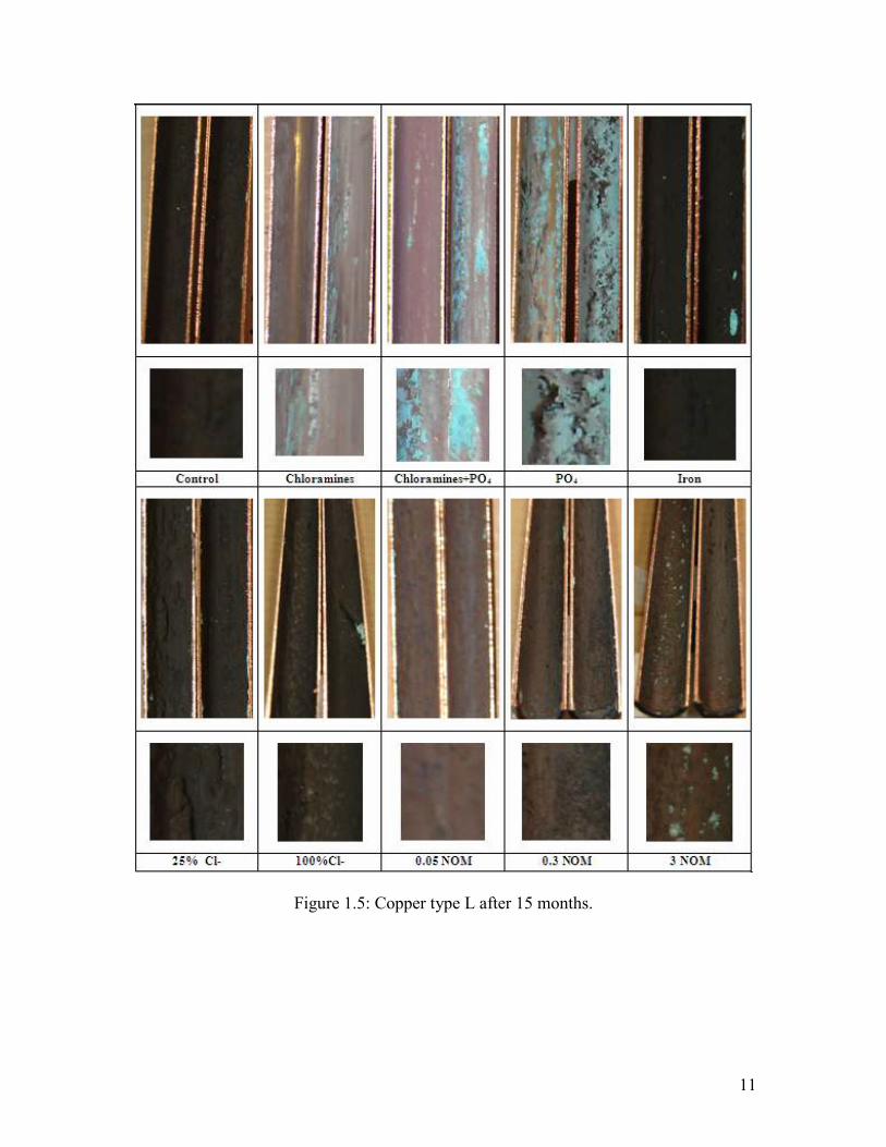
After 15 months the type M and L pipes were examined (Figure 1.4 to Figure 1.8). The

scale colors varied markedly dependent on exposure conditions. For the most part the

pipes were covered with a dark brown-black scale, but conditions with 3 mg/L NOM,

9

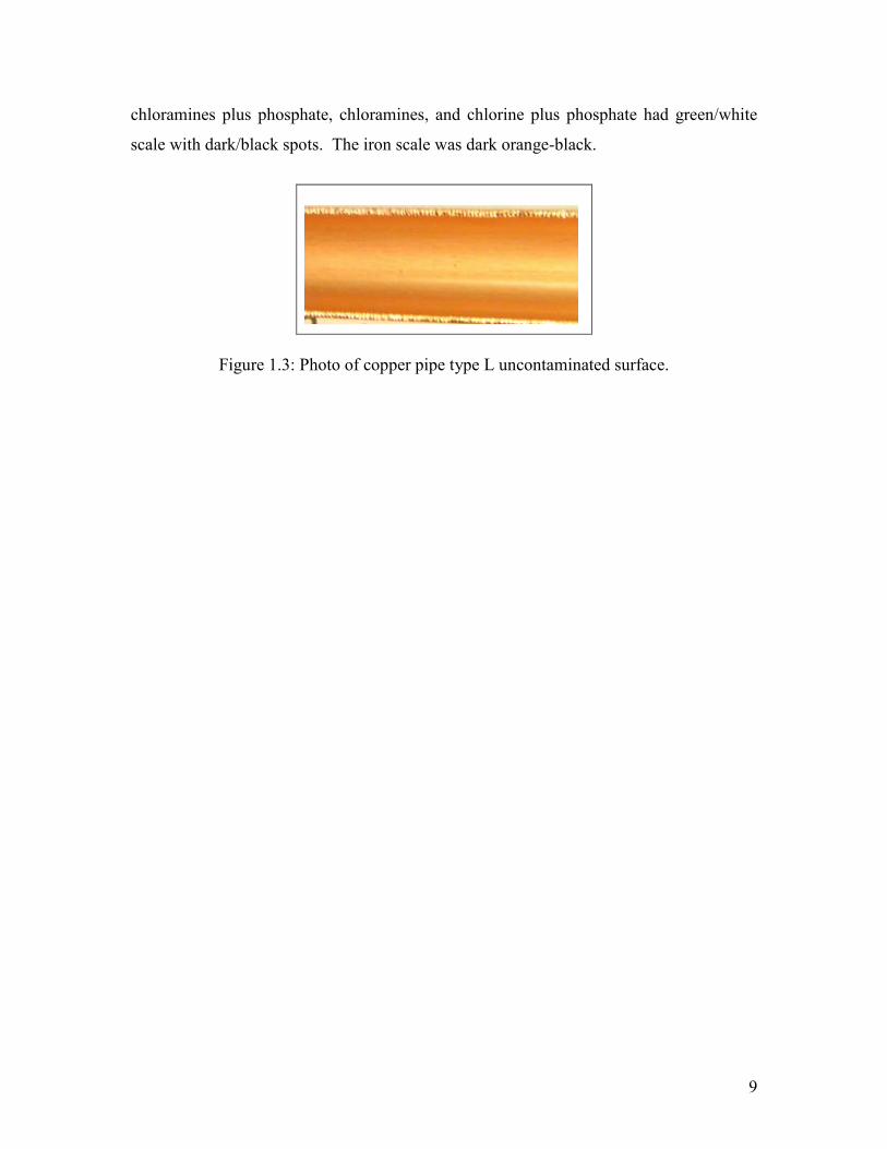
chloramines plus phosphate, chloramines, and chlorine plus phosphate had green/white

scale with dark/black spots. The iron scale was dark orange-black.

Figure 1.3: Photo of copper pipe type L uncontaminated surface.

10

Figure 1.4: Copper type M after 15 months.

11

Figure 1.5: Copper type L after 15 months.

12

Figure 1.6: Copper type M for the last 5 months after all metals other than copper were removed from the rig.

13

Figure 1.7: Copper type M after the last 3 months and removal of the other metals.

14

Figure 1.8: Copper type L ran for first 5 months (left)and copper type M ran for last 10 months (right).

15

Characterization of Pitting Propensity

Even though no pinholes developed in the copper pipes after 15 months of

experimentation, very serious pitting was nonetheless observed in many of the pipes.

Two sets of tubes were subject to detailed analysis at 11 and 15 months. Tubes exposed

to chloramine, chloramine plus phosphate, chlorine plus phosphate, and chlorine plus

phosphate had no pits deeper than 0.05 mm. This is completely consistent with

Marshall’s prediction based on electrochemistry that pitting in this water is driven by

chlorine and is inhibited by orthophosphate (Marshall et al., 2006). In contrast, all of the

other tubes had at least 5 pits that had eaten through more than 15% of a Type M pipe

wall thickness after just 11 months (Table 1.2). Indeed, the deepest pit on a tube exposed

to chlorine and iron had eaten through 55% of a Type M pipe wall in just 15 months.

Thus, while the experiment was a failure in terms of reproducing leaks and the extremely

rapid pitting described by Marshall, the test waters were still very aggressive to copper

and the analysis can support highly significant relative comparisons of pitting propensity

For a summary analysis of pitting and pit depth, the 5 worst pits on the 3’ sections of tube

were identified, and the range and average pit depth of these 5 pits were determined

(Table 1.2). After 15 months, the average depth of the 5 worst pits on the tube exposed

to iron particles were 96% deeper than the corresponding pits formed in the presence of

aluminum. Thus, iron particles were more detrimental than an equimolar dose of

aluminum in relation to pitting in this water.

With respect to NOM, levels of 0 mg/L (control), 0.05 and 0.3 mg/L had about the same

average pit depth (Figure 1.9). However, 3 mg/L NOM virtually eliminated pitting in the

first 11 months of the experiment and reduced pit depth by about 50% after 15 months.

Thus, while NOM did not completely stop pitting corrosion in this extremely aggressive

high pH water, it was still effective at slowing the rate of pit growth. It should be noted

that NOM tends to sorb to metal surfaces more weakly at higher pH than at lower pH, so

the current water is a situation in which effects of NOM on pitting are likely to be

minimized.

16

Finally, waters representing complete anion exchange treatment were worse than the

control water in terms of average pit depth, but better than the control water in terms of

maximum pit depth. In contrast, partial anion exchange treatment was worst of all. This

is consistent with a notion of an “optimally bad” ratio of Cl:SO4-2 in a given water

(Figure 1.9). Certainly all three waters were highly aggressive, but in this case it was an

intermediate ratio of Cl-:SO4-2 that was most aggressive in terms of the number of deep

pits.

Table 1.2: The range and average of 5 deepest pits on 3 feet long samples exposed for the indicated experimental time.

Penetration Range and average of 5 worst pits in parenthesis

Copper Control +25% Cl 100% Cl 0.05 NOM 0.3 NOM 3 NOM Iron 11 months

0.14-0.25 (0.16)

0.25-0.25 (0.25)

0.15-0.22 (0.19)

0.14-0.22 (0.16)

0.12-0.21 (0.14) All < 0.05

0.27-0.35 (0.29)

%depth 21 33 25 21 19 < 38 15 months

0.17-0.26 (0.19)

0.24-0.35 (0.28)

0.20-0.27 (0.24)

0.18-0.27 (0.21)

0.17-0.25 (0.18)

0.06-0.12 (0.09)

0.33-0.41 (0.37)

%depth 25 37 32 28 24 12 49

Figure 1.9: Photo of copper (type M) pipe surface (1 inch long) for 25% Cl- condition on the left and 0.3 NOM condition on the right.

17

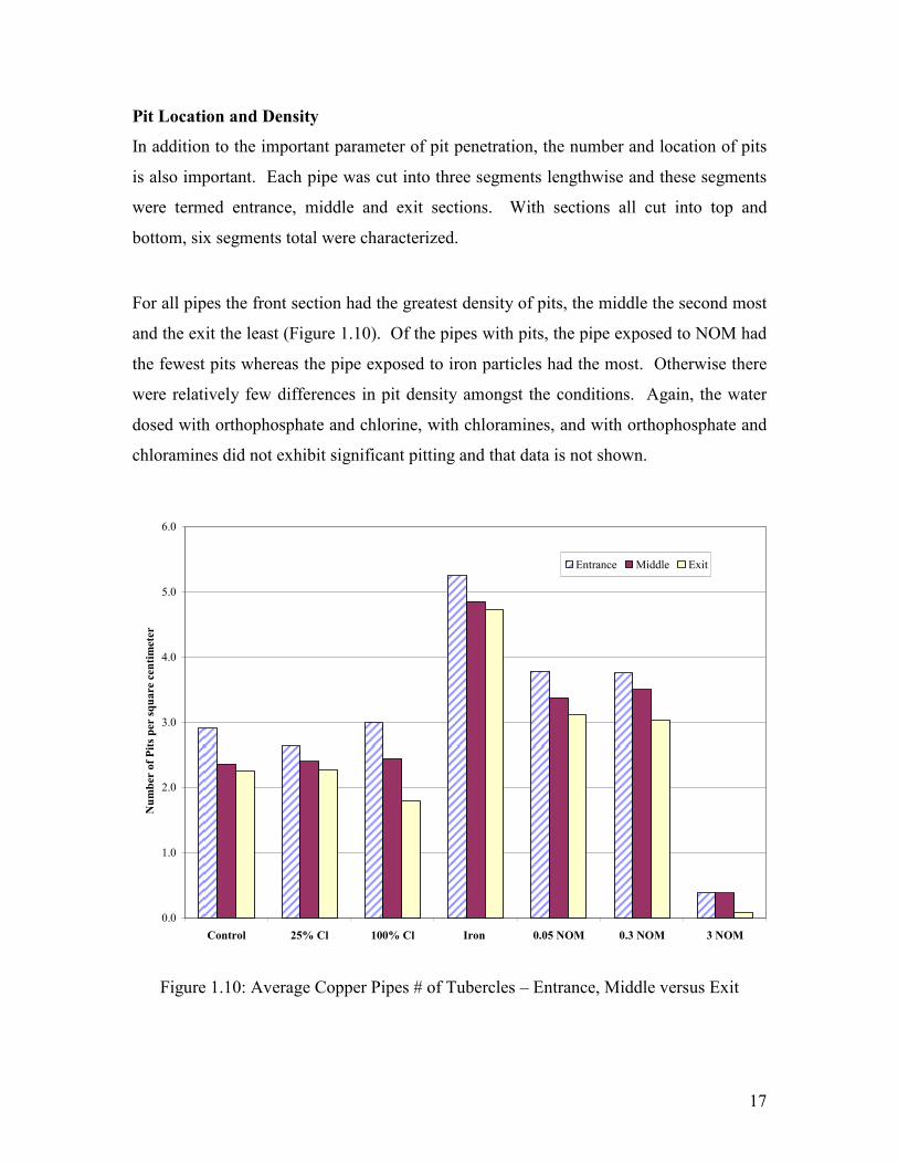
Pit Location and Density

In addition to the important parameter of pit penetration, the number and location of pits

is also important. Each pipe was cut into three segments lengthwise and these segments

were termed entrance, middle and exit sections. With sections all cut into top and

bottom, six segments total were characterized.

For all pipes the front section had the greatest density of pits, the middle the second most

and the exit the least (Figure 1.10). Of the pipes with pits, the pipe exposed to NOM had

the fewest pits whereas the pipe exposed to iron particles had the most. Otherwise there

were relatively few differences in pit density amongst the conditions. Again, the water

dosed with orthophosphate and chlorine, with chloramines, and with orthophosphate and

chloramines did not exhibit significant pitting and that data is not shown.

0.0

1.0

2.0

3.0

4.0

5.0

6.0

Control 25% Cl 100% Cl Iron 0.05 NOM 0.3 NOM 3 NOM

Number of Pits per square centimeter

Entrance Middle Exit

Figure 1.10: Average Copper Pipes # of Tubercles – Entrance, Middle versus Exit

18

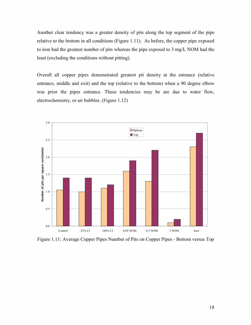
Another clear tendency was a greater density of pits along the top segment of the pipe

relative to the bottom in all conditions (Figure 1.11). As before, the copper pipe exposed

to iron had the greatest number of pits whereas the pipe exposed to 3 mg/L NOM had the

least (excluding the conditions without pitting).

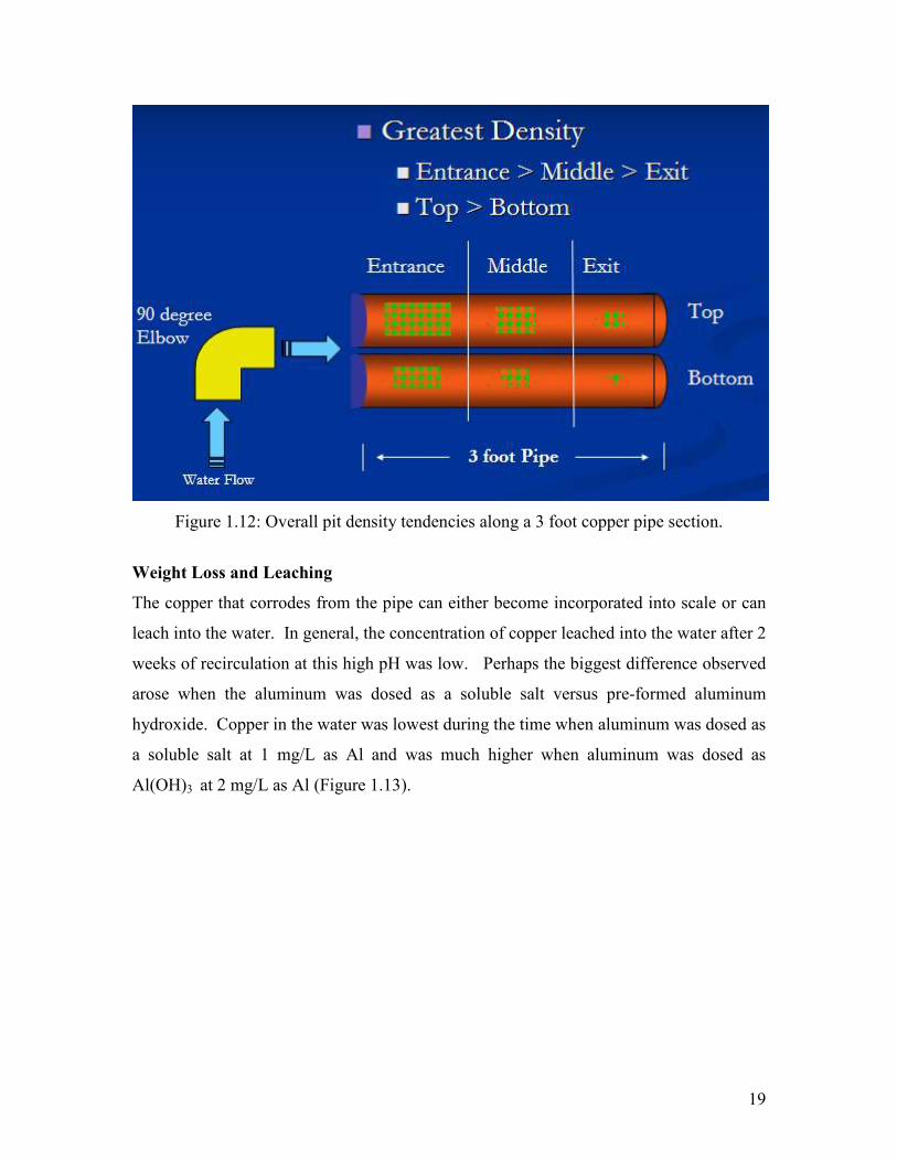
Overall all copper pipes demonstrated greatest pit density at the entrance (relative

entrance, middle and exit) and the top (relative to the bottom) when a 90 degree elbow

was prior the pipes entrance. These tendencies may be are due to water flow,

electrochemistry, or air bubbles. (Figure 1.12)

0.0

0.5

1.0

1.5

2.0

2.5

3.0

Control 25% Cl 100% Cl 0.05 NOM 0.3 NOM 3 NOM Iron

Number of pits per sq

uare

centimeter

Bpttom

Top

Figure 1.11: Average Copper Pipes Number of Pits on Copper Pipes - Bottom versus Top

19

Figure 1.12: Overall pit density tendencies along a 3 foot copper pipe section.

Weight Loss and Leaching

The copper that corrodes from the pipe can either become incorporated into scale or can

leach into the water. In general, the concentration of copper leached into the water after 2

weeks of recirculation at this high pH was low. Perhaps the biggest difference observed

arose when the aluminum was dosed as a soluble salt versus pre-formed aluminum

hydroxide. Copper in the water was lowest during the time when aluminum was dosed as

a soluble salt at 1 mg/L as Al and was much higher when aluminum was dosed as

Al(OH)3 at 2 mg/L as Al (Figure 1.13).

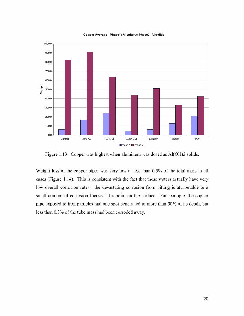
20

Copper Average - Phase1: Al salts vs Phase2: Al solids

0.0

100.0

200.0

300.0

400.0

500.0

600.0

700.0

800.0

900.0

1000.0

Control 25%>Cl 100% Cl 0.05NOM 0.3NOM 3NOM PO4

Cu, ppb

Phase 1 Phase 2

Figure 1.13: Copper was highest when aluminum was dosed as Al(OH)3 solids.

Weight loss of the copper pipes was very low at less than 0.3% of the total mass in all

cases (Figure 1.14). This is consistent with the fact that these waters actually have very

low overall corrosion rates-- the devastating corrosion from pitting is attributable to a

small amount of corrosion focused at a point on the surface. For example, the copper

pipe exposed to iron particles had one spot penetrated to more than 50% of its depth, but

less than 0.3% of the tube mass had been corroded away.

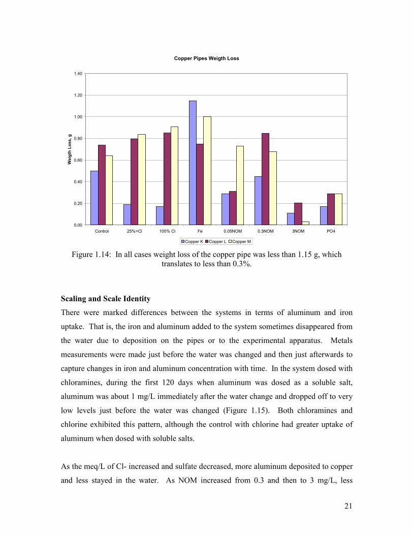
21

Copper Pipes Weigth Loss

0.00

0.20

0.40

0.60

0.80

1.00

1.20

1.40

Control 25%>Cl 100% Cl Fe 0.05NOM 0.3NOM 3NOM PO4

Weigth Loss, g

Copper K Copper L Copper M

Figure 1.14: In all cases weight loss of the copper pipe was less than 1.15 g, which translates to less than 0.3%.

Scaling and Scale Identity

There were marked differences between the systems in terms of aluminum and iron

uptake. That is, the iron and aluminum added to the system sometimes disappeared from

the water due to deposition on the pipes or to the experimental apparatus. Metals

measurements were made just before the water was changed and then just afterwards to

capture changes in iron and aluminum concentration with time. In the system dosed with

chloramines, during the first 120 days when aluminum was dosed as a soluble salt,

aluminum was about 1 mg/L immediately after the water change and dropped off to very

low levels just before the water was changed (Figure 1.15). Both chloramines and

chlorine exhibited this pattern, although the control with chlorine had greater uptake of

aluminum when dosed with soluble salts.

As the meq/L of Cl- increased and sulfate decreased, more aluminum deposited to copper

and less stayed in the water. As NOM increased from 0.3 and then to 3 mg/L, less

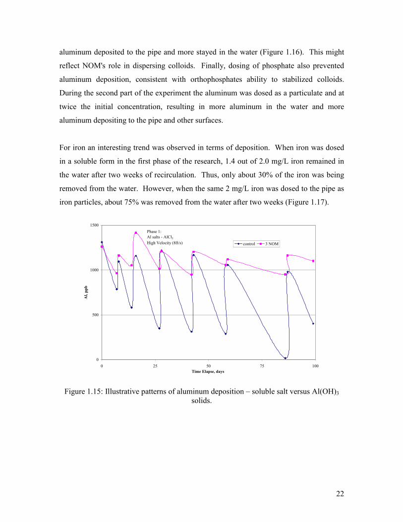
22

aluminum deposited to the pipe and more stayed in the water (Figure 1.16). This might

reflect NOM's role in dispersing colloids. Finally, dosing of phosphate also prevented

aluminum deposition, consistent with orthophosphates ability to stabilized colloids.

During the second part of the experiment the aluminum was dosed as a particulate and at

twice the initial concentration, resulting in more aluminum in the water and more

aluminum depositing to the pipe and other surfaces.

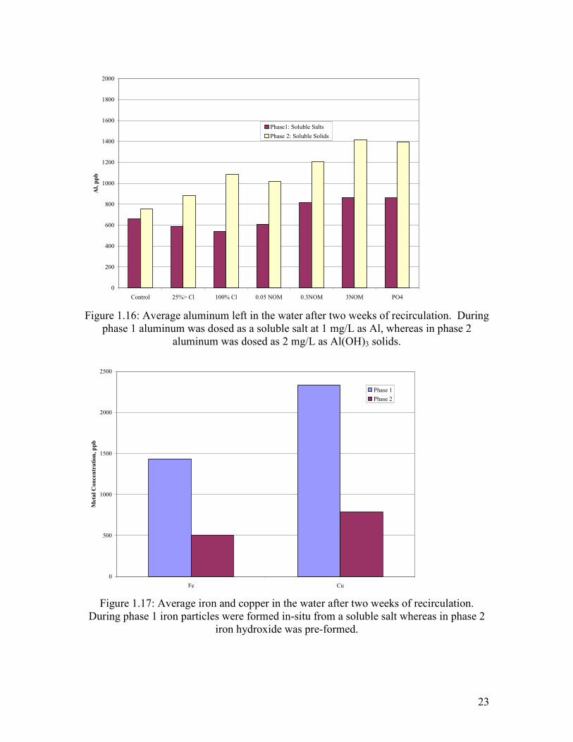
For iron an interesting trend was observed in terms of deposition. When iron was dosed

in a soluble form in the first phase of the research, 1.4 out of 2.0 mg/L iron remained in

the water after two weeks of recirculation. Thus, only about 30% of the iron was being

removed from the water. However, when the same 2 mg/L iron was dosed to the pipe as

iron particles, about 75% was removed from the water after two weeks (Figure 1.17).

0

500

1000

1500

0 25 50 75 100Time Elapse, days

Al, ppb

control 3 NOM

Phase 1:Al salts - AlCl3High Velocity (8ft/s)

Figure 1.15: Illustrative patterns of aluminum deposition – soluble salt versus Al(OH)3

solids.

23

0

200

400

600

800

1000

1200

1400

1600

1800

2000

Control 25%> Cl 100% Cl 0.05 NOM 0.3NOM 3NOM PO4

Al, ppb

Phase1: Soluble Salts

Phase 2: Soluble Solids

Figure 1.16: Average aluminum left in the water after two weeks of recirculation. During

phase 1 aluminum was dosed as a soluble salt at 1 mg/L as Al, whereas in phase 2 aluminum was dosed as 2 mg/L as Al(OH)3 solids.

0

500

1000

1500

2000

2500

Fe Cu

Metal Concentration, ppb

Phase 1

Phase 2

Figure 1.17: Average iron and copper in the water after two weeks of recirculation.

During phase 1 iron particles were formed in-situ from a soluble salt whereas in phase 2 iron hydroxide was pre-formed.

24

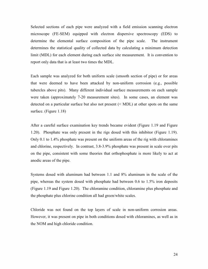
Selected sections of each pipe were analyzed with a field emission scanning electron

microscope (FE-SEM) equipped with electron dispersive spectroscopy (EDS) to

determine the elemental surface composition of the pipe scale. The instrument

determines the statistical quality of collected data by calculating a minimum detection

limit (MDL) for each element during each surface site measurement. It is convention to

report only data that is at least two times the MDL.

Each sample was analyzed for both uniform scale (smooth section of pipe) or for areas

that were deemed to have been attacked by non-uniform corrosion (e.g., possible

tubercles above pits). Many different individual surface measurements on each sample

were taken (approximately 7-20 measurement sites). In some cases, an element was

detected on a particular surface but also not present (< MDL) at other spots on the same

surface. (Figure 1.18)

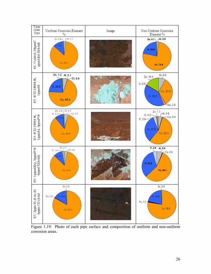
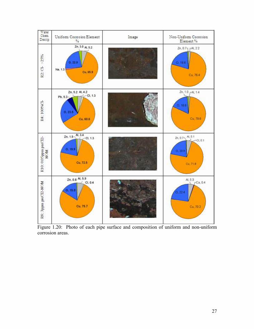
After a careful surface examination key trends became evident (Figure 1.19 and Figure

1.20). Phosphate was only present in the rigs dosed with this inhibitor (Figure 1.19).

Only 0.1 to 1.4% phosphate was present on the uniform areas of the rig with chloramines

and chlorine, respectively. In contrast, 3.8-3.9% phosphate was present in scale over pits

on the pipe, consistent with some theories that orthophosphate is more likely to act at

anodic areas of the pipe.

Systems dosed with aluminum had between 1.1 and 8% aluminum in the scale of the

pipe, whereas the system dosed with phosphate had between 0.6 to 1.5% iron deposits

(Figure 1.19 and Figure 1.20). The chloramine condition, chloramine plus phosphate and

the phosphate plus chlorine condition all had green/white scales.

Chloride was not found on the top layers of scale in non-uniform corrosion areas.

However, it was present on pipe in both conditions dosed with chloramines, as well as in

the NOM and high chloride condition.

25

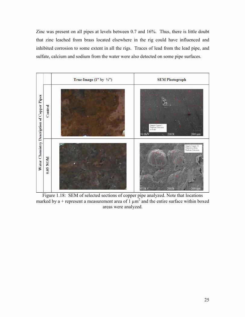
Zinc was present on all pipes at levels between 0.7 and 16%. Thus, there is little doubt

that zinc leached from brass located elsewhere in the rig could have influenced and

inhibited corrosion to some extent in all the rigs. Traces of lead from the lead pipe, and

sulfate, calcium and sodium from the water were also detected on some pipe surfaces.

Figure 1.18: SEM of selected sections of copper pipe analyzed. Note that locations

marked by a + represent a measurement area of 1 µm2 and the entire surface within boxed areas were analyzed.

26

Figure 1.19: Photo of each pipe surface and composition of uniform and non-uniform corrosion areas.

27

Figure 1.20: Photo of each pipe surface and composition of uniform and non-uniform corrosion areas.

28

Kinetics of Chlorine Decay

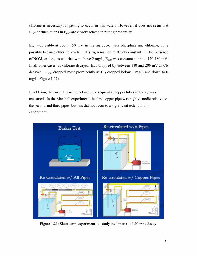
There were wide variations in the pattern of chlorine decay in the test waters during the

experiment. To better characterize the science behind this chlorine decay four types of

experiments were conducted including 1) beaker tests with the water but without pipes, 2)

tests in the recirculation rig at the end of the experiment but with no pipes present, 3)

circulation rig experiments with all the different pipe materials, and 4) circulation rig

experiments with only copper pipes present. Also, representative chlorine decay data

after 24 hours of circulation were obtained to characterize the trends of chlorine decay

during the experimental course. (Figure 1.21)

The beaker test was performed using a 3 liter chemically resistant plastic beaker while

slowly stirring at 250 rpm. Water was made up as described previously. The pH was

maintained at 9.4 and chlorine was maintained at 4 mg/L. Chlorine demand in all the

waters was very low, with less than 15% decay in 30 hours in all cases. There was some

initial rapid chlorine demand in the water dosed with 3 mg/L pre-chlorinated NOM in this

case. Kinetics were essentially zero order with constant loss of chlorine with time in all

waters (Figure 1.23).

The same test was repeated in the rigs after 1.25 years of experiment but after all the

metal pipes were removed. In this case the decay represents that observed in the water,

plus decay from contact with any oxide deposits left on the apparatus during rapid flow.

Results were similar to the batch test (Figure 1.23) with very low rates of chlorine decay.

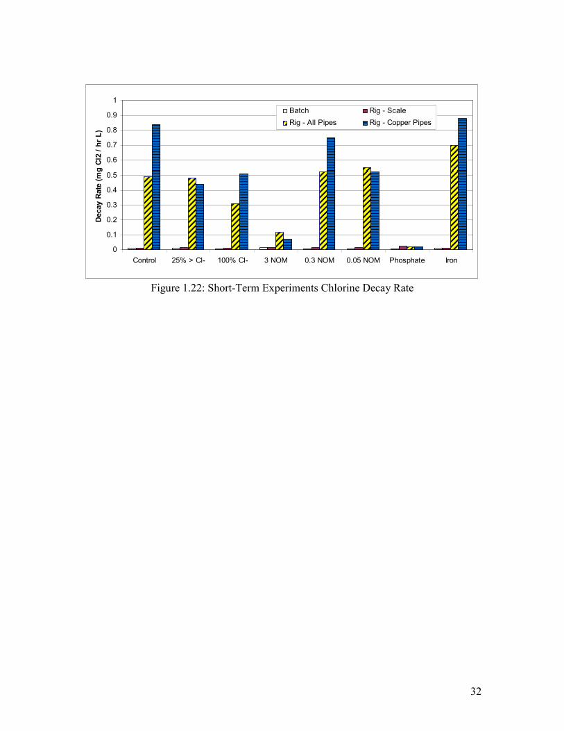
Overall, the system dosed with phosphate inhibitor had the most rapid decay.

When chlorine decay was characterized in the circulation rig with all the metal pipes

present, the situation changed markedly. Specifically, most pipes exhibited a high

chlorine demand and there were major differences amongst the rigs (Figure 1.23). Only

the water dosed with phosphate had chlorine decay rates which were about the same as in

the absence of pipes. Thus, decay rates in the presence of phosphate in the rigs without

metal pipe were highest and they were essentially unchanged with the metal pipes

present. However, the rig dosed with 3 mg/L NOM had the next lowest decay rate and

29

the rig dosed with iron particles had the highest rate. Clearly, the water was influencing

the chlorine demand exerted by the metal pipe surfaces present in the rig. Comparison to

the chlorine decay after all metal pipes but copper was removed from the rig suggest that

virtually all the demand was from copper pipe. That is, the extent and kinetics of

chlorine removal was about the same in this case versus the condition with all pipes, even

though only 1/3 of the copper surface was present. This similarity in decay rates might

be partly attributable to the presence of a new section of copper pipe in the rig at this

time.

By drawing a tangent to the initial decay curve, these trends can be summarized for all

four tests and waters tested, as illustrated in Figure 1.20 lower left graph (Figure 1.22).

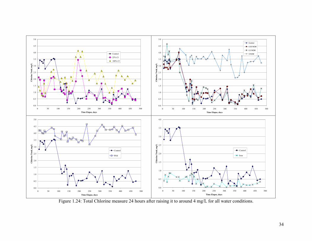
Throughout the experiment trends in chlorine decay were tracked by measurement of

residual chlorine after 24 hours (Figure 1.24). The control and lower levels of NOM

(0.05 and 0.3 NOM) increased chlorine decay after dosing of aluminum solids (after 4

months), from an average residual of 3-3.5 mg/L down to 0.5-1 mg/L. In contrast, water

conditions with the highest level of NOM or PO4 stayed higher than the other conditions

with an average of 3.5-4 mg/L during the entire course of the experiment.

In systems with variable Cl:SO4 ratio, the short term trend was different than the long

term trend. Early on, the highest amount of Cl- had a lower rate of chlorine decay, but by

the end of the experiment the opposite trend occurred. The highest rates of chlorine

decay were always observed in the rigs dosed with iron solids, and the decay rate in this

rig seemed to increase after 6½ months.

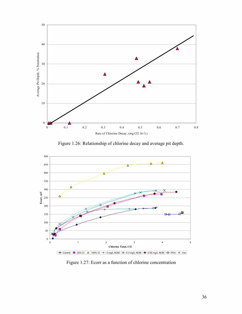
After examining the chlorine decay kinetics and compared to the average pit depth

(discussed early) a major tendency becomes clear. In general, waters with higher

chlorine decay rates are more susceptible to greater depth of pits. (Figure 1.26)

30

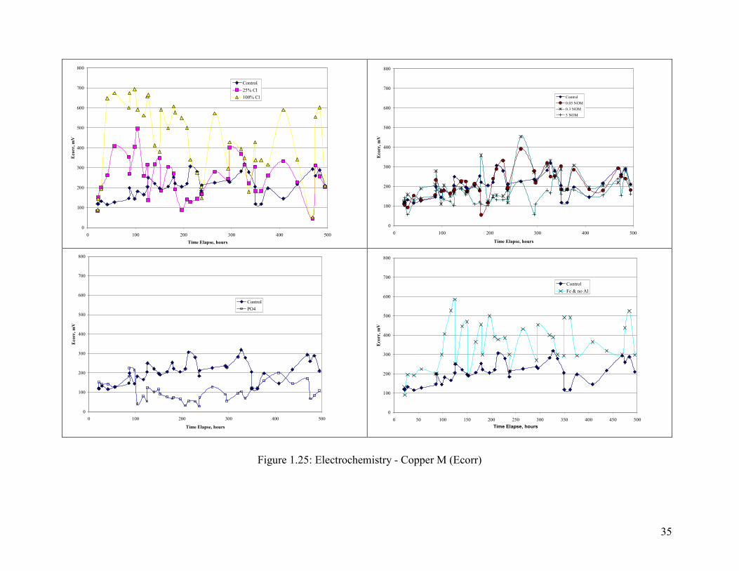
Electrochemistry of Pitting

Electrochemical potential, referred to simply as ECorr, is currently the most widely

applied and most successful means of tracking pitting propensity. An ECorr

measurement quantifies the electrical potential existing between a metal sample and a

reference electrode such as a Ag-AgCl. Pourbaix determined that when a new copper

was exposed into a water, ECorr would typically rise to within 100 mV vs. Ag-AgCl after a

period of days and then stabilize (Pourbaix, 1969). However, in waters that supported

copper pitting, ECorr would continue to rise over a period of months to a critical value at

which point pit initiation and propagation would have occurred. This overall trend is

collectively referred to as electrochemical rise. Mechanistically, ECorr rise results from

either acceleration of the cathodic reaction or a decrease in the anodic reaction. The fact

that ECorr rise is often correlated with pitting propensities offers support in favor of

Nguyen’s hypothesis that copper pitting reactions are under cathodic control; given that

factors which accelerate the cathodic reaction or localize anodic areas of attack increase

Ecorr and tend to encourage pitting.

In this case neither Ecorr rise and the absolute value of Ecorr was completely consistent

with trends in pitting. Specificially, as chloride content increased Ecorr also increased

(Figure 1.27), whereas pitting did not increase with the fraction of chloride in the water.

However, the next highest Ecorr, as well as a clear Ecorr rise occurred in the presence of

iron particles (Figure 1.27). For waters dosed with NOM, clear trends were not clear,

although the Ecorr in the presence of highest NOM tended to be lower than was observed

for other conditions (Figure 1.27). Ecorr in the presence of chloramines (not shown) and

chloramine/phosphate (Figure 1.27) were also very low, and these conditions did not pit.

The Ecorr was a strong function of the free chlorine content of the water (Figure 1.27).

For this test, total chlorine was monitored at different time intervals while it decayed, and

Ecorr was measured at the same time. This raises the possibility that Ecorr may be a good

overall indicator of pitting propensity simply because it is related to and is largely

controlled by the free chlorine concentration in the water. It is very clear that free

31

chlorine is necessary for pitting to occur in this water. However, it does not seem that

Ecorr or fluctuations in Ecorr are closely related to pitting propensity.

Ecorr was stable at about 150 mV in the rig dosed with phosphate and chlorine, quite

possibly because chlorine levels in this rig remained relatively constant. In the presence

of NOM, as long as chlorine was above 2 mg/L, Ecorr was constant at about 170-180 mV.

In all other cases, as chlorine decayed, Ecorr dropped by between 180 and 200 mV as Cl2

decayed. Ecorr dropped most prominently as Cl2 dropped below 1 mg/L and down to 0

mg/L (Figure 1.27).

In addition, the current flowing between the sequential copper tubes in the rig was

measured. In the Marshall experiment, the first copper pipe was highly anodic relative to

the second and third pipes, but this did not occur to a significant extent in this

experiment.

Figure 1.21: Short-term experiments to study the kinetics of chlorine decay.

32

0

0.1

0.2

0.3

0.4

0.5

0.6

0.7

0.8

0.9

1

Control 25% > Cl- 100% Cl- 3 NOM 0.3 NOM 0.05 NOM Phosphate Iron

Decay Rate (mg Cl2 / hr L)

Batch Rig - Scale

Rig - All Pipes Rig - Copper Pipes

Figure 1.22: Short-Term Experiments Chlorine Decay Rate

33

Batch - Glass Cointainer

1

2

3

4

5

6

0 10 20 30 40 50 60 70 80 90 100

Time Elapse, hrs

Chlorine Total, mg/L

Circulation Rigs Only with Tank Scale

1

2

3

4

5

0 10 20 30 40 50 60 70 80 90 100

Time Elapse, hrs

Chlorine Total, mg/L

Circulation Rigs - All Pipes

0

1

2

3

4

5

0 5 10 15 20 25 30

Time, hours

Chlorine Total, mg/L

Ciculation Rigs - Copper Pipes

0

1

2

3

4

5

0 2 4 6 8 10 12

Time Elapse, hrs

Chlorine Total, mg/L

Figure 1.23: Chlorine uptake in beaker tests (upper left), rig tests without pipe (upper right), in the rigs with all pipe present

(lower left), and in circulation rigs with copper only (lower right).

34

0.0

0.5

1.0

1.5

2.0

2.5

3.0

3.5

4.0

4.5

5.0

0 50 100 150 200 250 300 350 400 450 500

Time Elapse, days

Chlorine Total, mg/L

Control

25% Cl

100% Cl

0.0

0.5

1.0

1.5

2.0

2.5

3.0

3.5

4.0

4.5

5.0

0 50 100 150 200 250 300 350 400 450 500

Time Elapse, days

Chlorine Total, mg/L

Control

0.05 NOM

0.3 NOM

3 NOM

0.0

0.5

1.0

1.5

2.0

2.5

3.0

3.5

4.0

4.5

5.0

0 50 100 150 200 250 300 350 400 450 500

Time Elapse, days

Chlorine Total, mg/L

Control

PO4

0.0

0.5

1.0

1.5

2.0

2.5

3.0

3.5

4.0

0 50 100 150 200 250 300 350 400 450 500

Time Elapse, days

Chlorine Total, mg/L

Control

Iron

Figure 1.24: Total Chlorine measure 24 hours after raising it to around 4 mg/L for all water conditions.

35

Figure 1.25: Electrochemistry - Copper M (Ecorr)

0

100

200

300

400

500

600

700

800

0 100 200 300 400 500

Time Elapse, hours

Ecorr, mV

Control

25% Cl

100% Cl

0

100

200

300

400

500

600

700

800

0 100 200 300 400 500

Time Elapse, hours

Ecorr, mV

Control

0.05 NOM

0.3 NOM

3 NOM

0

100

200

300

400

500

600

700

800

0 100 200 300 400 500

Time Elapse, hours

Ecorr, mV

Control

PO4

0

100

200

300

400

500

600

700

800

0 50 100 150 200 250 300 350 400 450 500

Time Elapse, hours

Ecorr, mV

Control

Fe & no Al

36

Figure 1.27: Ecorr as a function of chlorine concentration

0

50

100

150

200

250

300

350

400

450

500

0 1 2 3 4 5

Chlorine Total, Cl2

Ecorr, mV

Control 25% Cl 100% Cl 3 mg/L NOM 0.3 mg/L NOM 0.05 mg/L NOM PO4 Iron

0

10

20

30

40

50

0 0.1 0.2 0.3 0.4 0.5 0.6 0.7 0.8

Rate of Chlorine Decay, (mg Cl2 /hr L)

Average Pit Depth, % Penetration

Figure 1.26: Relationship of chlorine decay and average pit depth.

37

DISCUSSION

Further consideration was given to the failure to produce very rapid formation of pinhole

leaks. To elaborate, no holes were created in any rig in the current work with 9’ of pipe

present in each, whereas the first of three 1’ sections in the Marshall study developed 8

leaks/ft. Moreover, overall tube weight loss in the current work was < 0.3%, whereas the

front tube in the Marshall study lost nearly 3% of its mass in 11 months. Thus, while the

current work reproduced severe pitting, it is believe that the overall corrosion conditions

were at least an order of magnitude less aggressive in this study than in the Marshall

study.

A retrospective analysis suggested at least 4 factors which have been involved either

alone or in part. First, zinc leaching from the brass in the rig may have inhibited pitting

on copper. Zinc is often cited as a cathodic inhibitor of non-uniform copper corrosion,

and its deposition on copper surfaces may have therefore reduced the growth rate of pits.

Even after the brass was completely removed from the rig at the end of year 1, deposits of

zinc from within the apparatus continued to dissolve, as evidenced by levels of 6-50 ppb

Zn+2 measured in the recirculated water months after the brass had been removed. The

potential inhibition of corrosion by zinc addition is a promising subject for future

research.

Secondly, in the current work, the first set of copper tubes in the flow path was almost at

the same Ecorr as the second and third samples. This is in marked constrast with the

experiment of Marshall and other recent tests conducted in this type of water, in which

the first section of copper tends to become highly anodic relative to the last sections. We

term this phenomenon “flow electrification,” and we suspect it tended to drive pitting in

the front section of copper in the Marshall study. Some preliminary experiments have

indicated that the presence of zinc in water stops flow electrification, which in turn, might

explain reduced rates of attack on copper in this work.

38

A third factor is that Cl2 levels dropped relatively rapidly in this apparatus (Figure 1.22)

when compared to the approach of Marshall, who maintained constant chlorine of 4

mg/L. Using the example with iron as illustrative, at t = 0 and 4 mg/L Cl2, the initial

chlorine decay rate is about 0.7 mg/L Cl2 per hour in this work. But because the Cl2 was

not replenished until 24 hours later and it often reached nearly 0 Cl2, the average rate of

Cl2 decay was 4 mg Cl2/L over 24 hours or 0.16 mg Cl2/L/hour. Thus, if the depth of pits

were directly proportional to Cl2 decay rates, pits would grow at 0.70/0.16 = 4.4 times

slower rate using the Cl2 dosing scheme in this work versus holding the Cl2 constant at 4

mg/L. This is clearly an important contributor and it might even be the only critical

difference. However, replenishing Cl2 twice each day during the last phase of the

experiment still did not reproduce rapid pitting as tracked by Ecorr.

Finally, it is possible that initial exposure of the copper to the higher flow rate or initial

use of soluble rather than particulate aluminum may have formed a protective layer on

the copper. It is possible this protective layer was somewhat resistant to pitting attack

even after aggressive conditions were restored.

CONCLUSIONS

In a water with a high pitting propensity attributable to free chlorine at high pH: 1) iron residuals caused more serious pitting than an equimolar level of aluminum

residuals 2) the form of the iron or aluminum, either initially soluble or initially particulate, can

lead to differences in deposition and might influence pit initiation 3) complete replacement of sulfate with chloride does not dramatically worsen pitting,

although it is believed that the ratio of chloride to sulfate is one key factor in pitting

4) levels of NOM between 0 and 0.3 mg/L NOM exhibited similar pitting severity; however, the presence of 3 mg/L NOM in the water inhibited pitting

5) the addition of orthophosphate reduced pitting propensity dramatically 6) substitution of chloramines for chlorine in water of this type reduced pitting severity Relative to results from previous research using water of the same approximate composition, less severe pitting was observed. This may be due to:

39

1) a different form of aluminum dosed in initial phases of testing (soluble instead of particulate)

2) presence of zinc inhibitor in the current test from corroding brass 3) lower levels of chlorine overall in the current experiment

40

REFERENCES Brongers M.P.H. (2002). Appendix K. Drinking Water and Sewer Systems in Corrosion

Costs and Preventative Strategies in the United States. Report FHWA-RD-01-156. U.S. Department of Transportation Federal Highway Administration.

Edwards, M. Corrosion Control in Water Distribution Systems. One of the Grand Engineering Challenges for the 21st Century. Edited by Simon Parsons, Richard Stuetz, Bruce Jefferson and Marc Edwards. Water Science and Technology p. 1-8 V. 49, N. 2 (2004a).

Edwards, M., J.C. Rushing, S. Kvech and S. Reiber. Assessing Copper Pinhole Leaks in Residential Plumbing. In “Scaling and Corrosion In Water and Wastewater Systems.” Edited by Simon Parsons, Richard Stuetz, Bruce Jefferson and Marc Edwards. Water Science and Technology p. 83-90 V. 49, N. 2 (2004b).

Edwards, M., J.F. Ferguson and S. Reiber. The Pitting Corrosion of Copper. Journal American Water Works Association. V. 86, No. 7, 74-90 (1994).

Marshall, B. Initiation, Propagation and Mitigation of Aluminum and Chlorine Induced Pitting Corrosion. Virginia Tech MS Thesis. (2004b).

Marshall, B. and M. Edwards. Phosphate Inhibition of Copper Pitting Corrosion. To be presented at the 2006 AWWA Water Quality Technology Conference. Denver, CO. 13 pages. (2006).

Marshutz, 2001. Hooked on Copper. Reeves Journal. Rushing, J.C., and M. Edwards. Effect of Aluminum Solids and Free Cl2 on Copper

Pitting. Corrosion Science. Volume 46, No. 12 pp 3069-3088 (2004).

41

CHAPTER 2: EFFECT OF ION EXCHANGE AND OTHER

TREATMENTS ON NON-UNIFORM CORROSION OF BRASS.

Nestor Murray and Marc Edwards

Department of Civil and Environmental Engineering Virginia Polytechnic Institute and State University

Blacksburg, VA 24061 USA

ABSTRACT. Although brass was attacked non-uniformally by an aggressive water at high pH and with high Cl2 content, no significant pitting occurred at any condition tested, even though pitting did occur for copper exposed to the exact same water. The implication is that zinc in the alloy may help to prevent non-uniform attack on copper and copper alloys.

INTRODUCTION

Plumbing products made from brass and other alloys are frequently used in valves,

pumps and other precision plumbing products. These materials also can legally contain

up to 8% lead by weight provided that they also pass certain performance standards. This

study examined the effects of water treatment on non-uniform corrosion of brass in an

aggressive high pH water with aluminum. The fraction of chloride and sulfate in the

water, amounts of natural organic matter (NOM), iron instead of aluminum, and

chloramines disinfectant were also examined as part of this evaluation.

Experimental Methods and Materials

The experimental setup, modifications to the waters and experimental timeline were

detailed in Chapter 1. The brass used in this work contained 0.09% lead, 63% copper and

36% zinc.

During the experiment in the rig with chloramines and chloramines plus phosphate,

nothing of significance appeared to be occurring with respect to non-uniform corrosion

early in the experiment. Therefore, in these two rigs significant deviations in the protocol

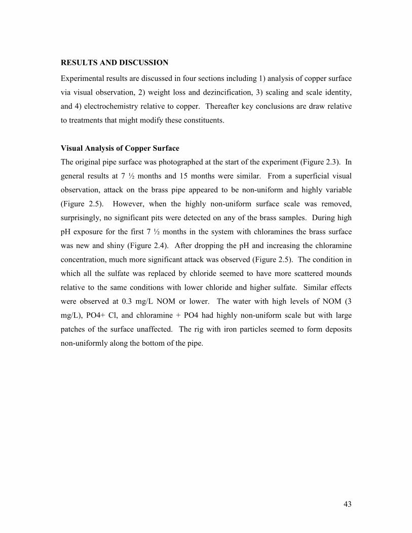
were tested including 1) very high levels of chloramines and 2) lower pH (Figure 2.1).

The molar ratio of chlorine to ammonia was always 4 to 1. However, the total chlorine

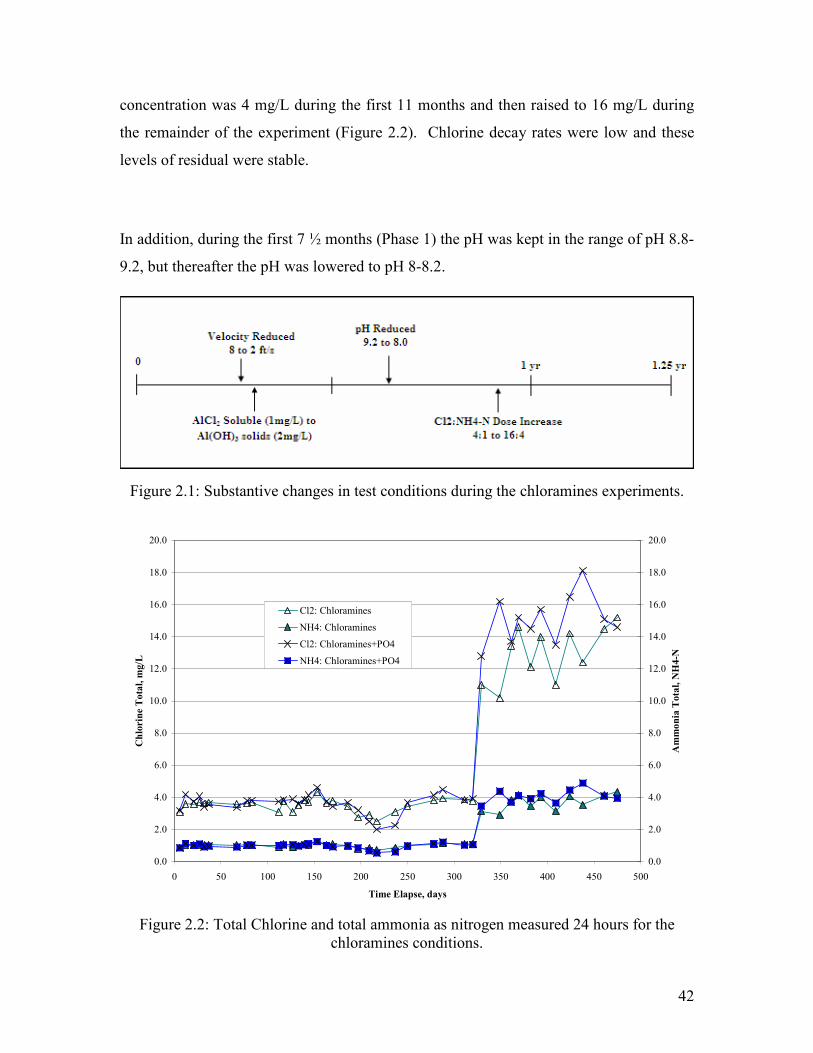
42

concentration was 4 mg/L during the first 11 months and then raised to 16 mg/L during

the remainder of the experiment (Figure 2.2). Chlorine decay rates were low and these

levels of residual were stable.

In addition, during the first 7 ½ months (Phase 1) the pH was kept in the range of pH 8.8-

9.2, but thereafter the pH was lowered to pH 8-8.2.

Figure 2.1: Substantive changes in test conditions during the chloramines experiments.

0.0

2.0

4.0

6.0

8.0

10.0

12.0

14.0

16.0

18.0

20.0

0 50 100 150 200 250 300 350 400 450 500

Time Elapse, days

Chlorine Total, mg/L

0.0

2.0

4.0

6.0

8.0

10.0

12.0

14.0

16.0

18.0

20.0

Ammonia Total, NH4-N

Cl2: Chloramines

NH4: Chloramines

Cl2: Chloramines+PO4

NH4: Chloramines+PO4

Figure 2.2: Total Chlorine and total ammonia as nitrogen measured 24 hours for the

chloramines conditions.

43

RESULTS AND DISCUSSION

Experimental results are discussed in four sections including 1) analysis of copper surface

via visual observation, 2) weight loss and dezincification, 3) scaling and scale identity,

and 4) electrochemistry relative to copper. Thereafter key conclusions are draw relative

to treatments that might modify these constituents.

Visual Analysis of Copper Surface

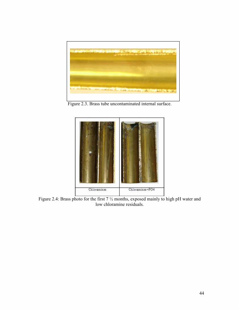
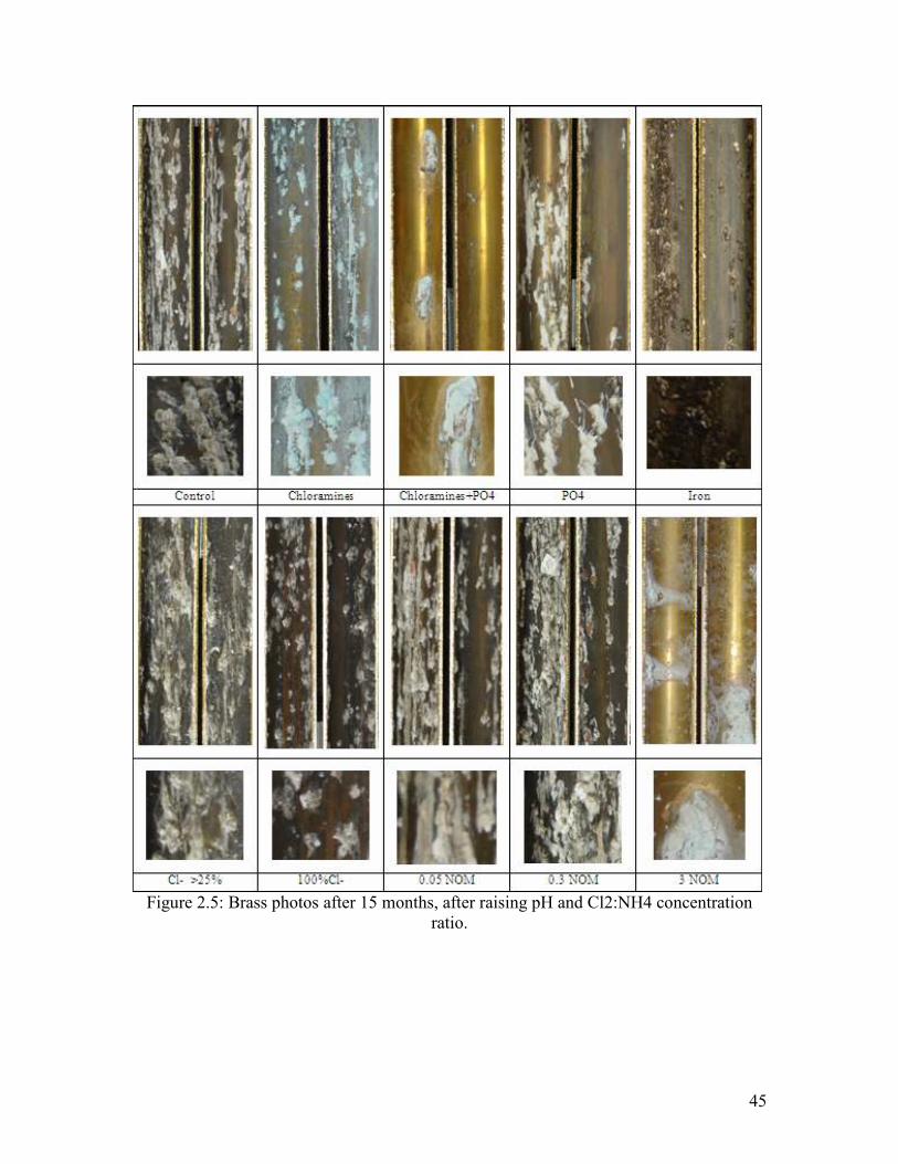
The original pipe surface was photographed at the start of the experiment (Figure 2.3). In

general results at 7 ½ months and 15 months were similar. From a superficial visual

observation, attack on the brass pipe appeared to be non-uniform and highly variable

(Figure 2.5). However, when the highly non-uniform surface scale was removed,

surprisingly, no significant pits were detected on any of the brass samples. During high

pH exposure for the first 7 ½ months in the system with chloramines the brass surface

was new and shiny (Figure 2.4). After dropping the pH and increasing the chloramine

concentration, much more significant attack was observed (Figure 2.5). The condition in

which all the sulfate was replaced by chloride seemed to have more scattered mounds

relative to the same conditions with lower chloride and higher sulfate. Similar effects

were observed at 0.3 mg/L NOM or lower. The water with high levels of NOM (3

mg/L), PO4+ Cl, and chloramine + PO4 had highly non-uniform scale but with large

patches of the surface unaffected. The rig with iron particles seemed to form deposits

non-uniformly along the bottom of the pipe.

44

Figure 2.3. Brass tube uncontaminated internal surface.

Figure 2.4: Brass photo for the first 7 ½ months, exposed mainly to high pH water and

low chloramine residuals.

45

Figure 2.5: Brass photos after 15 months, after raising pH and Cl2:NH4 concentration

ratio.

46

Weight Loss and Leaching

The zinc and copper that corrodes from the pipe can either become incorporated into

scale or can leach into the water. In general, the concentration of zinc leached into the

water after testing at pH 9.2 was high when compared to the second phase of experiments

at slightly higher pH (Figure 2.6). The exception was the system dosed with PO4, in

which zinc leaching markedly increased with the higher pH.

Despite the appearance of the samples which suggested an aggressive attack, only few of

the conditions exposed to chlorine had detectable weight loss (Figure 2.7). This is

consistent with the fact that these waters actually have very low overall corrosion rates.

0

20

40

60

80

100

120

140

160

Control 25% Cl- 100% Cl- 0.05 NOM 0.3 NOM 3 NOM PO4

Zinc, ppb

Phase 1Phase 2

Figure 2.6.A: Zinc leaching for all water conditions. Phase 1 ran for the first 7 months in which the upper pH limit was kept at 9.2; phase 2 ran the rest of the experiment with

an upper pH limit of 9.6.

47

0

200

400

600

800

1000

Iron Chloramines + PO4 Chloramines

Zinc, ppb

Phase 1

Phase 2

Figure 2.6.B: In the phase 1 for the iron condition iron soluble salts were added as in contrast with phase 2 were iron solids were added. In addition, for the chloramines

conditions phase 1 had high pH (9.2) and phase 2 had low pH (8.0).

0

0.2

0.4

0.6

0.8

1

1.2

1.4

Control Chloramines+PO4 Iron 3 NOM PO4

Weight Loss, grams

Figure 2.7. Weight loss of the brass pipes exposed to free chlorine at the end of the entire experiment. In all cases weight loss of the copper pipe was less than 1.2 g, which

translates to less than 0.3% of the pipe mass.

48

Scaling and Scale Identity

Selected sections of each pipe were analyzed with a field emission scanning electron

microscope (FE-SEM). The scale deposition was analyzed by acquiring a picture and

ESCA was used to identify major constituents (Figure 2.8).

Key trends became evident after a thorough evaluation (Figure 2.9 and Figure 2.10).

Areas of the pipe with scale were highly enriched in zinc relative to the alloyed metal,

whereas areas of the pipe without scale were deficient in aluminum.

Systems dosed with aluminum had between 6.2 and 8.4% aluminum in the scale of the

pipe, whereas the system dosed with phosphate and high NOM had 4.9 to 1.8%

aluminum deposits, respectively (Figure 2.9 and Figure 2.10). In contrast, systems dosed

with iron had only a small amount of iron 1.6% in the scale of the pipe. In the case of

non-uniform corrosion, aluminum traces were present in all conditions (2.7 to 7.2%) as

well as iron in the iron condition.

In both systems dosed with aluminum and iron, zinc (18.8 to 27%) and copper (39 to

54.7%) were important components of scale over the pipe surface. Conversely, iron and

chloramine conditions had higher zinc (40.8 and 33.3) and lower copper (19.7 and

23.4%) when compared to the rest of the conditions.

Chloride was found on the top layers of scale in non-uniform corrosion areas between 0.6

to 1.8%. However, it was not present on pipe in chloramine and low NOM (0.05 NOM)

conditions. Sulfate was found in the control, 25% chloride and chloramine conditions

ranging from 1.1 to 2.0%.

Lead was present only as a scale in the iron, PO4 and chloramine conditions as a trace

ranging form 3.4 to 11.4%. However, did only play an important a role on the non-

uniform scale for 100% chloride and iron conditions (3.5 and 5.4%).

49

Traces of sulfate, calcium and sodium from the water were also detected on some pipe

surfaces.

Figure 2.8: Example of the SEM selected sections of brass pipe analyzed. Note that

locations marked by a + represent a measurement area of 1 µm2.

50

Figure 2.9: Photo of each pipe surface and composition of uniform and non-uniform corrosion areas.

51

Figure 2.10: Photo of each pipe surface and composition of uniform and non-uniform corrosion areas.

52

Electrochemistry of Brass Corrosion

Several key measures of brass electrochemistry were tracked during the experiment.

Ecorr of the brass pipe relative to an AgCl reference electrode was, with few exceptions,

either stable or in decline throughout the experiment. This is consistent with the fact that

pitting did not occur.

The galvanic behavior of brass relative to copper was tested by connecting the brass pipe

to a copper pipe and measuring the voltage drop and current between the two (Figure

2.11, Figure 2.12 and Figure 2.13). A higher amount of Cl- relative to sulfate increased

the magnitude of the current between copper and brass, with the current acting to

sacrifice the brass. The presence of phosphate dramatically reduced the current, and

while NOM did not matter in the first part of the test, more NOM decreased the galvanic

current in the second part. The presence of iron increased currents relative to aluminum

(Figure 2.11). Trends in voltage were consistent with the current trends, in that a greater

voltage drop resulted in a greater current as described.

Chloramine results are discussed separately and in relation to the control with free

chlorine (Figure 2.14). In general, the voltage drops between the copper and lead in the

system with chloramine were very low throughout the experiment. Likewise, currents

and voltage between the two metals were also low. In general, the galvanic corrosion

between brass and copper seems to be driven by free chlorine and not chloramine, with

the main difference arising from chlorines ability to increase Ecorr of copper tube.

53

-200

-150

-100

-50

0

50

100

150

0 50 100 150 200 250 300

Time Elapse, days

Ecorr, mV

Control

25% Cl-

100% Cl-

-250

-200

-150

-100

-50

0

50

100

150

200

0 50 100 150 200 250 300

Time Elapse, days

Ecorr, mV

Control

0.05 NOM

0.3 NOM

3 NOM

-150

-100

-50

0

50

100

150

0 50 100 150 200 250 300

Time Elapse, days

Ecorr, mV

Control

PO4

-200

-100

0

100

200

300

400

500

0 50 100 150 200 250 300

Time Elapse, days

Ecorr, mV

Control

Iron

Figure 2.11: Brass pipe electrochemistry (Ecorr).

54

0

5

10

15

20

25

0 50 100 150 200 250 300 350 400

Time Elapse, days

Change in Current, microA

Control

25% Cl

100% Cl

0

5

10

15

20

0 50 100 150 200 250 300 350 400

Time Elapse, days

Change in Current, microA

Control

0.05 NOM

0.3 NOM

3 NOM

0

5

10

15

0 50 100 150 200 250 300 350 400

Time Elapse, days

Change in Current, microA

Control

PO4

0

5

10

15

20

25

0 50 100 150 200 250 300 350 400

Time Elapse, days

Change in Current, microA

Control

Iron

Figure 2.12: Brass pipe electrochemistry (change in voltage). Copper M versus Brass

55

0

100

200

300

400

500

600

700

800

0 50 100 150 200 250 300

Time Elapse, days

Voltage, mV

Control

25% Cl-

100% Cl-

0

100

200

300

400

500

600

0 50 100 150 200 250 300

Time Elapse, days

Voltage, mV

Control

0.05 NOM

0.3 NOM

3 NOM

0

100

200

300

400

0 50 100 150 200 250 300

Time Elapse, days

Voltage, mV

Control

PO4

0

100

200

300

400

500

600

0 50 100 150 200 250 300

Time Elapse, days

Voltage, mV

Control

Iron

Figure 2.13: Brass pipe electrochemistry (change in voltage). Copper M versus Brass

56

-150

-100

-50

0

50

100

0 50 100 150 200 250 300

Tiem Elapse, days

Ecorr, mV

ControlChloraminesChloramines+PO4

0

5

10

15

0 50 100 150 200 250 300 350

Time Elapse, days

Change in Current, microA

Control

Chloramines

Chloramines+PO4

0

100

200

300

400

0 50 100 150 200 250 300

Time Elapse, days

Voltage, mV

Control

Chloramines

Chloramines+PO4

Figure 2.14: Electrochemistry of Brass: Ecorr (Top), Change in Current (Middle) and

Voltage (Bottom) measure against copper type M.

57

CONCLUSIONS

In a water with a high pitting propensity attributable to free chlorine at high pH: 1) brass was attacked non-uniformally, no significant pitting occurred at any condition tested

2) zinc in the alloy may help to prevent non-uniform attack copper alloys. 3) the galvanic corrosion between brass and copper seems to be driven by free chlorine and not chloramines

Key Conclusion: No significant pitting was occurred at any of the conditions.

58

CHAPTER 3: LEAD LEACHING FROM IN-LINE BRASS DEVICES:

A CRITICAL EVALUATION OF THE EXISTING STANDARD

Abhijeet Dudi†, Marc Edwards †, Michael Schock‡, and Nestor Murray†

† Department of Civil and Environmental Engineering Virginia Polytechnic Institute and State University

Blacksburg, VA 24061 USA

‡ Environmental Protection Agency Water Supply and Water Resources Division

National Risk Management Research Laboratory USEPA, Cincinnati, OH 45268

ABSTRACT. The ANSI/NSF 61, Section 8 standard is relied on to protect the public from in-line brass plumbing products that might leach excessive levels of lead to potable water. Experiments were conducted to examine the practical rigor of this test. Contrary to expectations, the test was not highly protective of public health. Rather, it was determined that small devices made of pure lead- which pose an obvious public hazard- can easily pass the leaching protocol. Reforms are needed to help prevent such unacceptable outcomes in the future. Brass devices passing the test can contribute to lead levels at the tap in residences, schools and other buildings.

INTRODUCTION

A crisis of confidence arising from excessive lead in potable water of the nation’s capital

(Nakamura, 2004, Edwards et al., 2004a,b) has prompted a comprehensive national

review of lead standards. It is widely accepted that minimizing the extent of lead

leaching to drinking water from plumbing materials is a worthy public health goal and the

EPA Lead and Copper Rule (LCR) has achieved great progress in this area (Federal

Register, 1991). The amount of lead leached to public drinking water is a function of two

key factors that are under societal control. The first factor is the type of plumbing

material used, because some plumbing products have a relatively high tendency to

contaminate drinking water with lead. The second factor is the corrosivity of the water

supply that contacts plumbing products. Achieving the goal of very low lead in potable

water requires progress in both areas.

59

The EPA LCR has been designed to assess the lead leaching tendency of public water

supply in the context of existing plumbing. Lead present in the one liter "first draw" EPA

LCR sample can come from: 1) lead present in the source water, 2) lead leached to water

as it quickly passes through service lines at high flow rates, and 3) lead leached to water

as it contacts the home plumbing system during prolonged stagnation (Figure 3.1). The

EPA LCR also requires monitoring of lead leaving the treatment plant and has very

limited sampling provisions to detect “spikes” of lead that might build up in water from

prolonged stagnation in service lines (Edwards and Dudi, 2004b). If 90% of first draw

samples are not below the 15 ppb lead action limit, the LCR prescribes steps to minimize

corrosivity of the water. For example, by manipulating the chemistry of public drinking

water through adjustment of pH, alkalinity, or by addition of corrosion inhibitors such as

orthophosphate, it is often possible to greatly reduce leaching of lead to public water

supplies at relatively modest cost (Schock, 1989a; Schock et al, 1996; Edwards, 2002a).

Such corrosion control steps can often reduce lead leaching to water from many lead-

bearing plumbing products including pure lead pipe, lead solders and brass.

Some progress has been made phasing out potentially harmful plumbing products. Pure

lead pipe, leaded solders and brass with > 8% lead content were deemed such a potential

hazard, they were explicitly banned in the 1986 SDWA as amended in 1996 (Federal

Register, 2000). Recently, progress has been driven by Proposition 65 in California,

which has led to use of very low lead brass residential water meters and required a more

stringent standard for lead discharge from consumer faucets. Proposition 65 has also

impacted standards for products that are available nationally (Maas et. al., 2002a-e).

However, the definition of “lead free” brass still allows sale of devices containing up to

8% lead by weight as long as they are in compliance with performance standards

established in accordance with 42 U.S.C. 300g-6(e) (EPA, 2005)

60

Figure 3.1: The lead and copper rule requires sampling at the treatment plant (LCR 1) and

in first draw samples from consumers’ tap (LCR 3). Some sampling is recommended of

service lines (LCR 2). NSF section 8 and section 9 are performance standards that

attempt to insure that plumbing devices do not have a tendency to leach high levels of

lead to potable water.

61

To illustrate the potential magnitude of the problem, we note that a typical gate valve has

at least 100 g of brass that could uniformly corrode away before the product failed. At

5% lead content, the lead leached to water from corrosion could contaminate every drop

of water (e.g., increase the concentration to the 15 ppb action limit) that would be used by

a typical family of four in a year. Of course, this amount of brass corrosion does not

occur in a year, but is spread over the product lifetime. In typical domestic plumbing

system configurations, multiple brass devices are often installed between the water main

and the water taps in the home. Thus, there can be an additive effect. They also give

potential for rather unpredictable “spikes” of lead in drinking water coming from the tap.

These spikes could be attributable to a combination of the water that sat inside these

devices during stagnation, plus sloughing off of particulate (precipitated or corroded)

material during stagnation and flow.

These considerations illustrate a societal need for a test that prevents installation of brass

products that could release excessive amounts of soluble or particulate lead to water.

What are the desirable characteristics of a test? On the practical side, those selling

plumbing products are correct to argue that the test should be of reasonable duration and

expense. If the test was too expensive or required too much time, improved plumbing

products could be excluded from market, which is not in the public interest. It is also

critical that the test be reproducible in different product testing laboratories around the

country and at different times. Finally, it is critical that the test be prospective, such that

products leaching problematic levels of lead can be excluded from the pool of products

that is installed in homes (or schools) before they pose a direct public health threat or

difficulty with regulatory compliance. Obviously, many of the home or institutional

plumbing products in question are not visible or even readily accessible once installed, so

a “recall” of dangerous products would be practically impossible.

62

It must also be kept in mind that under the Lead and Copper Rule, for large water systems

(serving over a population of 50,000), the target 90th percentile value is not 0.015 mg/L.

Rather, the target is “optimization” or minimization of a lead release, which can be

viewed as a more stringent goal. Nonetheless, standards that “allow” brass devices to

contribute significant lead can cause corrosion control treatment burdens and difficulty in

meeting LCR 90th percentile requirements for corrosion control.

Some have argued that the EPA Lead and Copper Rule (LCR) itself will protect the

public from leaded brass products that are currently legal. This argument logically fails

for many reasons. First, the EPA LCR would have to be modified extensively to quantify

lead leaching from leaded brass devices, since at present the LCR does not 1) intend to

make sure that homes are sampled with every possible type of plumbing product

configuration, 2) attempt to document the presence of specific types of leaded brass

products present in the homes which are sampled in the EPA LCR, and 3) purposefully

detect spikes of lead that might occur from leaded brass installed near the service lines.

Additionally, only a very small percentage of residences are sampled by the LCR, which

leaves detection of unusual problems in homes up to individual consumers. Testing of

new in-line products using something like the LCR would require installation of

potentially dangerous untested products in consumers’ homes, sampling according to

some new protocol as yet undeveloped, and exposing consumers to potentially harmful

levels of lead throughout the test. In short, the LCR was not designed, nor can it

rationally be modified, to protect the public from specific potentially harmful plumbing

products.

63

For new brass plumbing products, the two currently accepted performance standards

designed to protect public health include NSF 61 Section 9 and NSF 61 Section 8 (Table

1). Plumbing products that pass NSF Section 9 have explicit recognition from the EPA in

terms of limiting lead leaching to water (EPA, 2004). All other brass devices fall under

NSF 61 Section 8 (Table 3.1) and are termed “in-line” devices. There is presently no

national legal requirement that in-line brass devices meet either NSF 61 Section 8 or

Section 9 standards. However, 44 states had legislation requiring conformance to these

standards by 2001, and the remaining states had intentions to do so (ASDWA, 2001). Of

course, enforcing the standards requires continued vigilance and verification. For

instance, recent surveys in the state of Pennsylvania have shown that prohibited lead:tin

solder are widely available for use in plumbing installations and repairs (Ziegler 2001;

Crowell 2002; Hendrix 2004; Wade 2003) and similar issues can be expected for leaded

brass devices.

Table 3.1: Comparison of NSF 61 Section 8 and Section 9.

NSF 61-Section 8 NSF 61-Section 9 Stated Coverage

In-line devices, or devices installed on the service line downstream of the endpoint

devices.

Endpoint devices, or devices that typically contact the last liter of the distribution system (e.g., the first

draw sample) Illustrative brass devices covered

Backflow preventor, valves and fittings (e.g., building valves, check valves, compression

fittings), corporation stops, meter couplings, meter stops, water

meters

Lavatory and kitchen faucets, drinking water fountains, supply stops and endpoint control valves.

Illustrative brass devices

specifically exempted

Temperature and pressure relief valves, valves with hose thread

outlets

Bath and shower valves, roman tub valves, backflow prevention devices, faucets with a hose tread spout end, faucets that are self-closing, metering

or electronically activated.

64

While many in the drinking water industry are familiar with the general reputation of

NSF 61 in certifying plumbing products as safe for drinking water usage, detailed

knowledge of the test protocol is not readily accessible or widely understood. Few

appreciate that there are important differences between the test protocols for end-point

devices such as faucets versus those for in-line devices as detailed by Hazan et al. (1994).

In-line devices are tested in two waters henceforth termed the “NSF pH 5” and “NSF pH

10” water. After the devices are exposed to the test waters for up to 14 days

conditioning, lead leached to the test water is quantified after a 12-16 hour stagnation

period. The measured concentration of lead from the test is then normalized to

“determine the level of contaminants projected “at the tap” based on the level of

contaminants identified during laboratory analysis” (e.g. NSF, 2000). If the normalized

concentration is less than 15 parts per billion (ppb) with both test waters, the product

passes the protocol and can be NSF certified, as long as the product also contains less

than 8% lead by weight as specified by law (EPA, 2004).

Products that pass the test can be found labeled "ANSI/NSF 61-8 Clean Water for Our

Future” in the marketplace, and other prominent displays indicate that devices offered for

sale have passed the standard (Figure 3.2). A purchaser would be further reassured to

read NSF literature which indicates the NSF 61 Section 8 standard was developed by a

consortium of: NSF International, The American Water Works Association Research

Foundation, the Association of State Drinking Water Administrators, The American

Water Works Association with support from The U.S. Environmental Protection Agency

under cooperative agreement #CR-812144 (e.g. NSF, 2000). In the preface on page v of

the original 1988 NSF 61 Standard, it is stated: “Standard 61 was developed to establish

minimum requirements for the control of potential adverse human health effects from

products which contact drinking water.” The key point is that members of the public and

the water industry expect that NSF 61 certification prevents public use of products that

would release excessive concentrations of lead to drinking water.

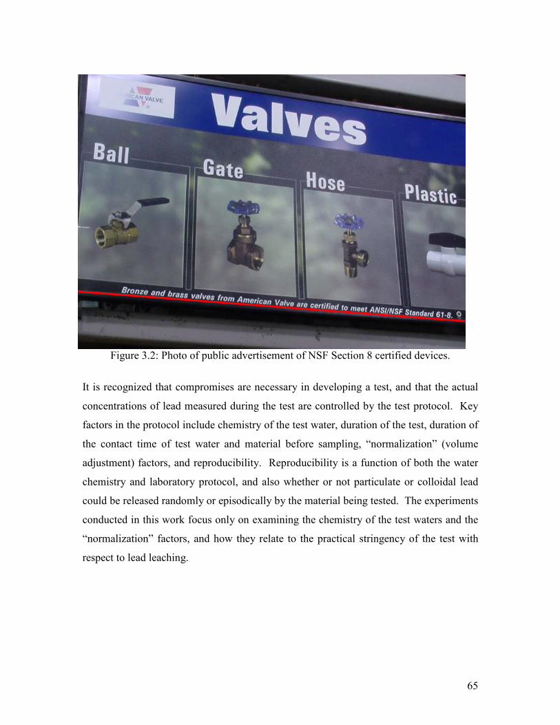
65

Figure 3.2: Photo of public advertisement of NSF Section 8 certified devices.

It is recognized that compromises are necessary in developing a test, and that the actual

concentrations of lead measured during the test are controlled by the test protocol. Key

factors in the protocol include chemistry of the test water, duration of the test, duration of

the contact time of test water and material before sampling, “normalization” (volume

adjustment) factors, and reproducibility. Reproducibility is a function of both the water

chemistry and laboratory protocol, and also whether or not particulate or colloidal lead

could be released randomly or episodically by the material being tested. The experiments

conducted in this work focus only on examining the chemistry of the test waters and the

“normalization” factors, and how they relate to the practical stringency of the test with

respect to lead leaching.

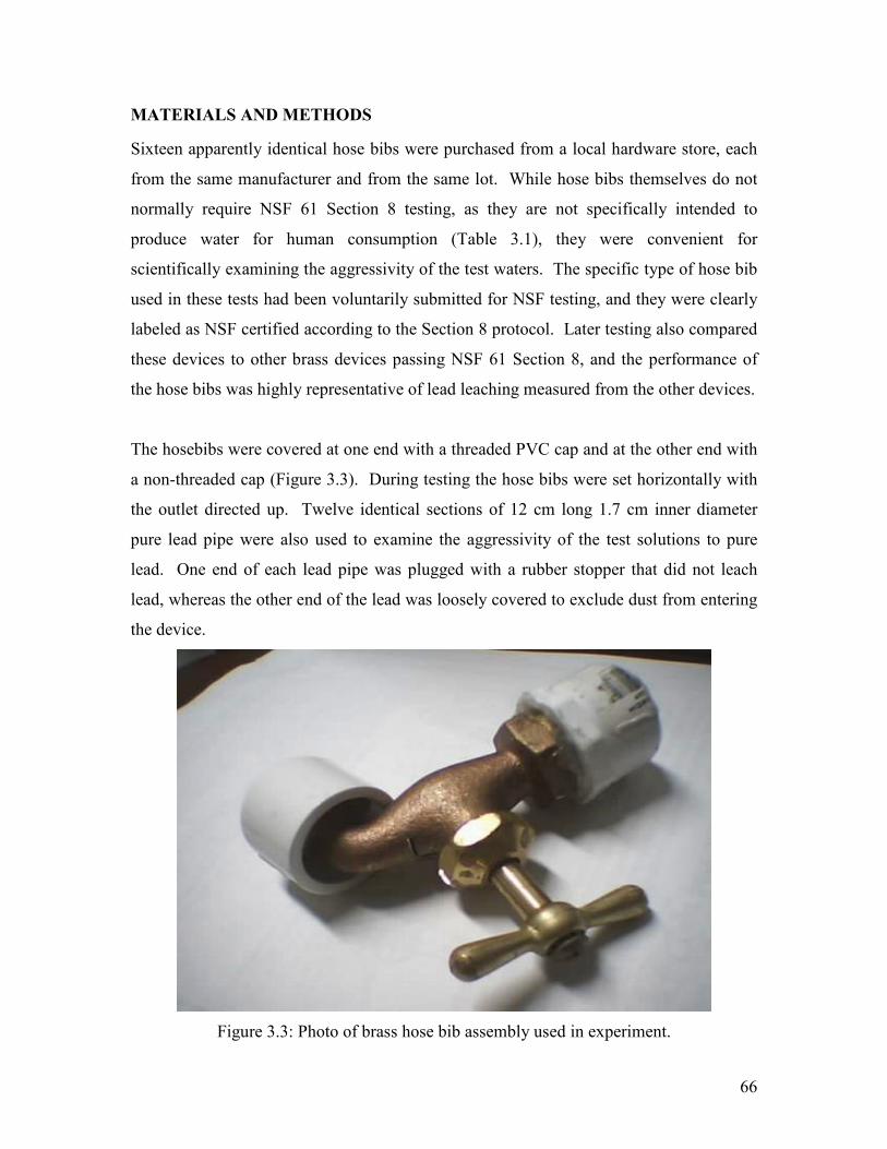
66

MATERIALS AND METHODS

Sixteen apparently identical hose bibs were purchased from a local hardware store, each

from the same manufacturer and from the same lot. While hose bibs themselves do not

normally require NSF 61 Section 8 testing, as they are not specifically intended to

produce water for human consumption (Table 3.1), they were convenient for

scientifically examining the aggressivity of the test waters. The specific type of hose bib

used in these tests had been voluntarily submitted for NSF testing, and they were clearly

labeled as NSF certified according to the Section 8 protocol. Later testing also compared

these devices to other brass devices passing NSF 61 Section 8, and the performance of

the hose bibs was highly representative of lead leaching measured from the other devices.

The hosebibs were covered at one end with a threaded PVC cap and at the other end with

a non-threaded cap (Figure 3.3). During testing the hose bibs were set horizontally with

the outlet directed up. Twelve identical sections of 12 cm long 1.7 cm inner diameter

pure lead pipe were also used to examine the aggressivity of the test solutions to pure

lead. One end of each lead pipe was plugged with a rubber stopper that did not leach

lead, whereas the other end of the lead was loosely covered to exclude dust from entering

the device.

Figure 3.3: Photo of brass hose bib assembly used in experiment.

67

The leaded samples were rinsed twice with de-ionized water, and then rinsed twice and

later filled with water from one of four different solutions:

1) NSF pH 5.0 water: 203.25 mg/L MgCl2 (51.82 mg/L as Mg) and 347.25

mg/L NaH2PO4 (77 mg/L as P) with 2 mg/L as Cl2.

2) NSF pH 5.0 water without phosphate: same recipe as pH 5 water but

without NaH2PO4.

3) NSF pH 10 water: 476.75 mg/L sodium borate (110.4 mg/L-B) at pH 10

dosed with 2 mg/L as Cl2.

4) Aerated NSF pH 10 water: Same recipe as NSF pH 10 water but aerated for

an hour, then readjusted to pH 10.

For comparison, the same leaded materials were exposed to a relatively non-aggressive

tap water containing 30.5 mg/L alkalinity as CaCO3, pH 8.6, 40 mg/L of Cl- and 50 mg/L

of SO4-2. In each case, chlorine was added from fresh solutions of reagent grade sodium

hypochlorite (bleach) when fresh solutions were made up weekly. Each condition was

tested in triplicate. pH was precisely adjusted to the target value using 1 N HCl or 1 N

NaOH.

Water was changed in the devices as per the published ANSI/NSF 61, Section 8 schedule.

Basically, after the product is rinsed as described above, the protocol calls for a minimum

of 24 hours between water changes and allows up to 10 water changes over a time period

up to 14 days. In this work, water in the device was changed every 24 hours, except

when samples were taken for lead analysis after the 2nd, 9th, 25th and 58th days of

exposure. All sampling was after a 16 hour stagnation time. The same schedule was

followed for the pure lead pipes except that the experiments were terminated after the

25th day. On occasion, samples collected from the pure lead pipes were passed through a

0.45 µm pore size nylon syringe filter to quantify soluble lead.

68

Another short-term experiment was designed to test the ability of the NSF protocol to

detect plumbing products that would pose an obvious lead hazard. For the test, an “in-

line device” was made of pure lead that held 6.3 mL of water. This device was then

tested according to the NSF protocol using the pH 5 water with only 2 days of exposure,

which is allowable under NSF 61 but which maximizes the likelihood a product would

fail. Samples were collected from the pipe after a 13 hour dwell time and were preserved

with 2% nitric acid and held for at least 28 hours before analysis.

All samples were analyzed for phosphorous, lead, copper, and zinc using a Jobin Yvon

Ultima Induced Coupled Plasma-Emission Spectroscopy (ICP-ES) as per standard

method 3120 B (APHA, 1998).

RESULTS AND DISCUSSION

Results are presented in five sections including: 1) considerations of test water chemistry,

2) effect of the phosphate on leaching propensity of the NSF pH 5.0 water, 3) effect of

CO2 influx on leaching propensity of the NSF pH 10 water, 4) ability of the NSF protocol

to detect an obviously flawed product, and 5) retrospective analysis and

recommendations.

Consideration of Test Water Chemistry.

Many believe that the two NSF Section 8 test waters were specifically designed to extract

a very high amount of lead from a product. To the extent this is true, the test would be

more protective, since concentrations of lead leached to the test water would be much

higher than would ever be encountered in practice. But close examination of the test

water chemistry and methodology reveal potential problems with that belief.

69

For the NSF pH 5 water, the concern is the presence of 2.5 mM of orthophosphate. This

is a level of orthophosphate expressed, in common units, as 77 mg/L as P or 240 mg/L as

PO4. Orthophosphate is present in the test solution to act as a pH buffer, but it is also

specifically added to drinking water to reduce lead leaching (e.g., Schock et al, 1996).

Nationally, about half of all large public utilities add phosphate corrosion inhibitors to

their drinking water (McNeill & Edwards, 2002). The concentration of orthophosphate in

the NSF pH 5.0 water is between 20-100 times higher than the level of phosphate

commonly added to water by utilities to control lead leaching to drinking water.

Solubility models have been useful in predicting changes to lead leaching in response to

phosphate inhibitor dosing. The models predict, and field evidence supports, that even

low doses of phosphate dramatically reduce lead solubility even at pH 5 (Figure 3.4);

therefore, it is expected that the presence of the phosphate would reduce lead leaching to

the test solution (Schock, 1989a; Schock el al, 1996; Edwards et. al., 1999 and

2002a&b). For example, a water at pH 5 in equilibrium with the atmosphere can hold

millions of ppb lead in solution, but the same water with 77 mg P/L orthophosphate

present can hold only a few hundred of micrograms per liter (ppb) of lead in solution.

This suggests that the NSF pH 5 water may not be as aggressive as is commonly

believed, due to the very high concentrations of inhibitor that are present.

70

Considering the NSF pH 10 water, which is a pure water buffered with a high

concentration of borate, confidential discussions with laboratories that conduct such

testing revealed that this water is of highly variable aggressiveness. Laboratories

observed that generally products fail more easily in “fresh” solutions, whereas they pass

more easily in older or “seasoned” pH 10 waters. The test protocol itself does not specify

age of the solutions to be used, or the type of containers used (i.e., open or closed to the

atmosphere), which could affect CO2 exchange rates with the water. Some labs use fresh

waters while others make up large quantities of water to use over a period of months. If

it were proven that this difference in approach caused any variability in results, it would

be problematic since the same product might fail in one lab and then pass the test in

others. It also has been observed that high concentrations of borate, such as are used in

the NSF pH 10 test water, can provide corrosion inhibition through unspecified

mechanisms (Butler and Ison, 1966)

The notion that storage of the test water would alter corrosivity is anticipated based on

potential dissolution of carbon dioxide from air to the alkaline solution. Lead solubility

is extremely sensitive to presence of CO2 in this pH range. In fact, over a reasonable

range of CO2 that might dissolve into the water in a period of months, solubility models

predict that influx of even small amounts of CO2 to the NSF pH 10 water would

dramatically decrease lead leaching (Figure 3.5). This is consistent with water utility

experiences, in that high pH and low carbonate waters are known to be highly non-

aggressive to lead leaching based on both solubility models and practical data (Schock,

1980; Schock et al, 1983; Dodrill & Edwards, 1995; Edwards et. al., 1999). In fact, the

high pH and low alkalinity condition is specifically targeted to control lead leaching in

many water systems.

Experiments in the following two sections examine the lead leaching ability of the NSF

pH 5.0 water and pH 10 waters.

71

Figure 3.4: Equilibrium solubility of lead as a function of phosphate concentration at pH 5.0. Dissolved inorganic carbon is assumed to be that present at equilibrium with air

(0.14 mg/L).

Figure 3.5: Equilibrium solubility of lead as a function of dissolved inorganic carbon

(DIC) at pH 10.

72

Effect of Phosphate on Lead Leaching Propensity of the NSF pH 5 Water.

The concentration of copper, zinc and lead leached from the brass hose bibs and pure lead

pipes were studied as a function of time. Results after 9 days of dump and fill exposure

are selected as illustrative. The phosphate (i.e., inhibitor) in pH 5 water markedly

decreased leaching of lead from both brass (Figure 3.6) and pure lead pipe (Figure 3.7).

For instance, for brass on the 9th day of exposure, average release from the water without

phosphate in brass hose bibs was 0.185 mg/L, consistent with the relatively high

aggressiveness of distilled water noted in Gardels & Sorg (1989). In the NSF pH 5 water

but with the orthophosphate, lead leaching was 5 times lower at 0.038 mg/L (Figure 3.6).

This difference is deemed significant at greater than 99% confidence using a t-test

assuming equal variance (P = 0.005). As a further point of comparison, leaching of lead

to the relatively non-aggressive tap water was 0.16 mg/L. Thus, the non-aggressive tap

water actually leached more than 4 times less lead than did the supposedly aggressive

NSF pH 5 water. Clearly, the NSF pH 5 is actually not aggressive in the context of lead

leaching from leaded brass.

Not surprisingly, levels of lead leached from pure lead pipes during the test were orders

of magnitude higher than for brass (Figure 3.7), consistent with the hazardous nature of

lead pipe in practical situations. More than 25 times less lead was leached to the NSF pH

5 water relative to the same water without phosphate. The NSF pH 5 water leached 3.5

times less lead than did the non-aggressive tap water at pH 8.5. Most of the lead leached

from the pure lead pipes in these tests was particulate, and in the non-aggressive tap

water soluble lead was virtually undetectable.

73

The presence of phosphate in the NSF pH 5 water decreased lead leaching, but its effects

on copper were complex in comparison to both field and laboratory experience (Schock,

et al., 1995; Schock & Fox, 2001). In this test, it increased copper leaching by 14 times

relative to the same samples for pH 5 without phosphate buffer (Figure 3.8). This is the

result of a complex interaction of low pH with low dissolved inorganic carbon (DIC)

concentration, which is consistent with several research studies. The general expectation

(Edwards et. al., 1996 and 2002a; Lytle & Schock, 1996) is that copper phosphate solids

are not predicted to form in low DIC waters at this very low pH, and the phosphate buffer

tended to reduce the final pH of water at the end of the test (pH = 5.2) relative to the

same water without buffer (pH = 7.77). Since the final pH was lower the phosphate

could exert no inhibiting action on copper leaching, and the NSF pH 5.0 water is more

aggressive for copper relative to the same water without phosphate (Edwards et. al.,

2002a). This effect should not be confused with well established benefits from phosphate

inhibitors in reducing copper leaching in high alkalinity waters at circa neutral pH.

The effect of test duration was also studied (Figure 3.9). As expected, a higher amount of

lead was leached from each device at the start of experiment, and it gradually decreased

with time as the sample aged. However, in the presence of phosphate buffer, lead

leaching was relatively low even from the very first sample collected and aging was less

of an issue. In fact, in the presence of phosphate buffer, lead leaching was less than 0.05

mg/L in just 9 days. The opposite effect was observed for copper in the presence of

phosphate. Specifically, with phosphate the copper surface did not passivate, whereas in

the absence of phosphate relatively low amounts of copper were leached from the start of

the experiment (Figure 3.9). Leaching of zinc from the brass was relatively insensitive to

the level of phosphorous, and leaching decreased markedly with exposure time (data not

shown).

74

Figure 3.6: Amount of lead leached after an overnight stagnation after 9 days from brass hose bibs. Result is average of triplicate samples. All error bars in this paper denote

90% confidence intervals.

Average Amount of lead leached at the end of 9th day

0

0.05

0.1

0.15

0.2

0.25

NSF pH 5 Water NSF pH 5 Water

without P

Tap Water

Lead leached (mg/L)

75

Figure 3.7: Total and soluble lead leached after an overnight stagnation from the pure lead pipes after 9 days of dump and fill.

Total Lead

0

20

40

60

80

100

120

140

160

180

200

NSF pH 5 NSF pH 5

Without

Phosphorous

NSF pH 10 Tap Water

Type of water

Amount of lead leached (mg/l)

2.44 mg/L

62.9 mg/L

8.69 mg/L

175 mg/L

Soluble Lead

0

10

20

30

40

50

60

70

NSF pH 5 NSF pH 5

Without

Phosphorous

NSF pH 10 Tap Water

Type of water

Amount of lead leached (mg/l) .

0.638 mg/L

28.7 mg/L

0 mg/L

53.7 mg/L

76

Figure 3.8: Amount of copper leached after an overnight stagnation after 9 days of dump

and fill for NSF pH 5 water with and without phosphate.

Total Copper

0

0.5

1

1.5

2

2.5

3

3.5

4

4.5

NSF pH 5 Water NSF pH 5 Water without P

Total C

opper (m

g/L)

77

Total Lead

0

0.5

1

1.5

2

0 10 20 30 40 50 60

Days

Amount of Lead Leached (mg/L)

NSF pH 5 Water

NSF pH 5 Water without Phosphate

Figure 3.9: Lead and copper leached after an overnight stagnation as a function of time

for brass hose bibs.

Total Copper

0

1

2

3

4

0 10 20 30 40 50 60

Days

Amount of Copper Leached (mg/L)

NSF pH 5 Water

NSF pH 5 Water without Phosphate

78

Effect of aeration on Lead Leaching Propensity of the NSF pH 10 Water.

After one hour of mild aeration, the NSF pH 10 water had a final pH of 9.2 and an

inorganic carbon content of 37 mg/L. This is only about 30% of the inorganic carbon

expected for a water equilibrated at pH 9.2 CO2 with the atmosphere, so the water

remains highly undersaturated and could have held much more CO2 (Lytle et al, 1998).

This aerated solution was deemed a reasonable compromise between a fresh solution and

what might normally be encountered after months of storage in open containers in

practice, since the aeration increased the inorganic carbon in this highly buffered solution

while only slightly lowering the pH. The pH of this water was re-adjusted back to 10

with freshly prepared NaOH in order to isolate the effect of inorganic carbon alone on the

results. The same water prepared without aeration had a pH of 10 and a typical inorganic

carbon content of 1.0 mg/L. Solubility curves predict that lead solubility (and therefore

soluble lead leaching) would actually be minimized at only 4 mg/L inorganic carbon and

maximized at 0 mg/L carbon (Figure 3.10).

Inorganic carbon can have very complex effects on lead leaching as a function of

exposure time, since carbonate can form soluble complexes with lead in solution but

carbonate can also form highly insoluble lead solids on the surface of the plumbing

material. Since it takes time to form the insoluble lead solids, and the kinetics relate to

both carbonate and hydroxide ion activities, the presence of inorganic carbon can

increase lead leaching for a time before ultimately decreasing lead leaching (Schock &

Gardels; 1983; Schock, 1989b; Schock et. al. 1996; Edwards & McNeill, 2002b).

Consistent with that expectation, the first measurement (Figure 8) demonstrated higher

lead leaching in the aerated water (high carbonate) relative to the same water without

aeration (lower carbonate). But by the 9th day of testing the two results were nearly

identical, and at every time thereafter the aerated water with higher carbonate contained

much less lead. In this case copper showed nearly identical trends to lead (Figure 3.10),

as would be expected given short term importance of soluble cupric carbonate complexes

relative to the longer term importance of insoluble cupric oxide and hydroxycarbonate

solids on the pipe wall (Schock, et. al., 1995; Edwards et. al., 1996).

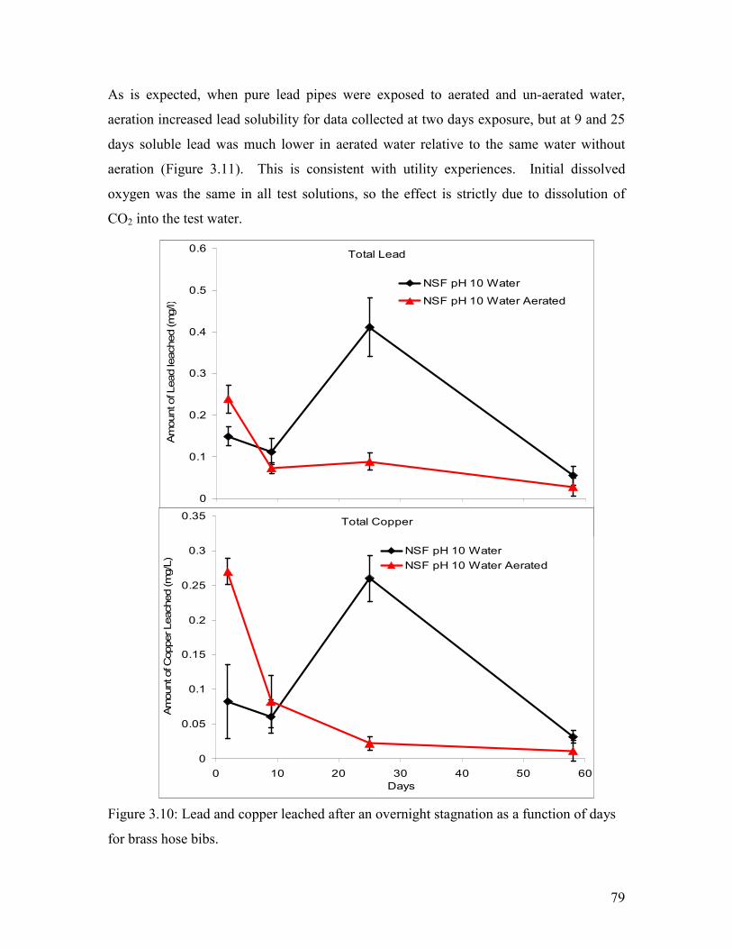
79

As is expected, when pure lead pipes were exposed to aerated and un-aerated water,

aeration increased lead solubility for data collected at two days exposure, but at 9 and 25

days soluble lead was much lower in aerated water relative to the same water without

aeration (Figure 3.11). This is consistent with utility experiences. Initial dissolved

oxygen was the same in all test solutions, so the effect is strictly due to dissolution of

CO2 into the test water.

Figure 3.10: Lead and copper leached after an overnight stagnation as a function of days

for brass hose bibs.

Total Lead

0

0.1

0.2

0.3

0.4

0.5

0.6

0 10 20 30 40 50 60

Days

Amount of Lead leached (mg/l)

NSF pH 10 Water

NSF pH 10 Water Aerated

Total Copper

0

0.05

0.1

0.15

0.2

0.25

0.3

0.35

0 10 20 30 40 50 60

Days

Amount of Copper Leached (mg/L)

NSF pH 10 Water

NSF pH 10 Water Aerated

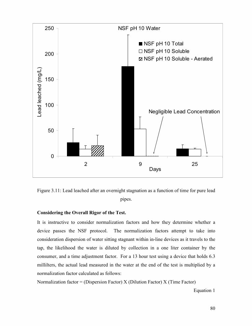
80

Figure 3.11: Lead leached after an overnight stagnation as a function of time for pure lead

pipes.

Considering the Overall Rigor of the Test.

It is instructive to consider normalization factors and how they determine whether a

device passes the NSF protocol. The normalization factors attempt to take into

consideration dispersion of water sitting stagnant within in-line devices as it travels to the

tap, the likelihood the water is diluted by collection in a one liter container by the

consumer, and a time adjustment factor. For a 13 hour test using a device that holds 6.3

millilters, the actual lead measured in the water at the end of the test is multiplied by a

normalization factor calculated as follows:

Normalization factor = (Dispersion Factor) X (Dilution Factor) X (Time Factor)

Equation 1

NSF pH 10 Water

0

50

100

150

200

250

2 9 25Days

Lead leached (mg/L)

NSF pH 10 Total

NSF pH 10 Soluble

NSF pH 10 Soluble - Aerated

Negligible Lead Concentration

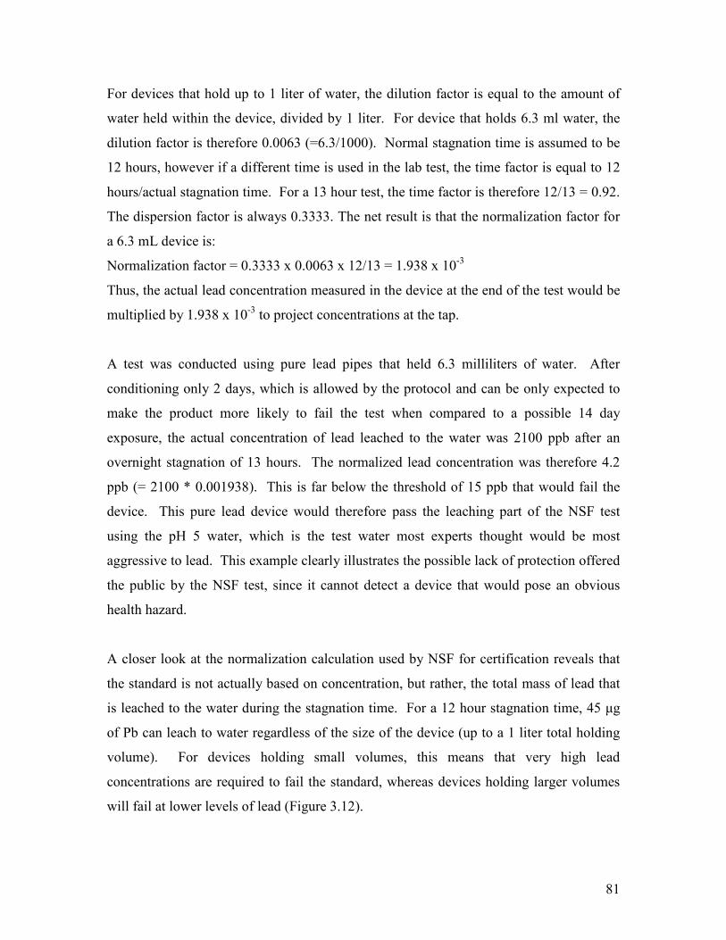
81

For devices that hold up to 1 liter of water, the dilution factor is equal to the amount of

water held within the device, divided by 1 liter. For device that holds 6.3 ml water, the

dilution factor is therefore 0.0063 (=6.3/1000). Normal stagnation time is assumed to be

12 hours, however if a different time is used in the lab test, the time factor is equal to 12

hours/actual stagnation time. For a 13 hour test, the time factor is therefore 12/13 = 0.92.

The dispersion factor is always 0.3333. The net result is that the normalization factor for

a 6.3 mL device is:

Normalization factor = 0.3333 x 0.0063 x 12/13 = 1.938 x 10-3

Thus, the actual lead concentration measured in the device at the end of the test would be

multiplied by 1.938 x 10-3 to project concentrations at the tap.

A test was conducted using pure lead pipes that held 6.3 milliliters of water. After

conditioning only 2 days, which is allowed by the protocol and can be only expected to

make the product more likely to fail the test when compared to a possible 14 day

exposure, the actual concentration of lead leached to the water was 2100 ppb after an

overnight stagnation of 13 hours. The normalized lead concentration was therefore 4.2

ppb (= 2100 * 0.001938). This is far below the threshold of 15 ppb that would fail the

device. This pure lead device would therefore pass the leaching part of the NSF test

using the pH 5 water, which is the test water most experts thought would be most

aggressive to lead. This example clearly illustrates the possible lack of protection offered

the public by the NSF test, since it cannot detect a device that would pose an obvious

health hazard.

A closer look at the normalization calculation used by NSF for certification reveals that

the standard is not actually based on concentration, but rather, the total mass of lead that

is leached to the water during the stagnation time. For a 12 hour stagnation time, 45 µg

of Pb can leach to water regardless of the size of the device (up to a 1 liter total holding

volume). For devices holding small volumes, this means that very high lead

concentrations are required to fail the standard, whereas devices holding larger volumes

will fail at lower levels of lead (Figure 3.12).

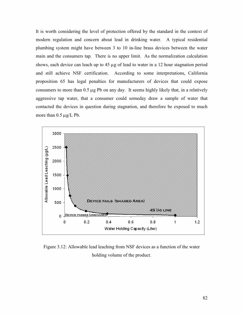
82

It is worth considering the level of protection offered by the standard in the context of

modern regulation and concern about lead in drinking water. A typical residential

plumbing system might have between 3 to 10 in-line brass devices between the water

main and the consumers tap. There is no upper limit. As the normalization calculation

shows, each device can leach up to 45 µg of lead to water in a 12 hour stagnation period

and still achieve NSF certification. According to some interpretations, California

proposition 65 has legal penalties for manufacturers of devices that could expose

consumers to more than 0.5 µg Pb on any day. It seems highly likely that, in a relatively

aggressive tap water, that a consumer could someday draw a sample of water that

contacted the devices in question during stagnation, and therefore be exposed to much

more than 0.5 µg/L Pb.

Figure 3.12: Allowable lead leaching from NSF devices as a function of the water

holding volume of the product.

83

Retrospective Evaluation and Recommendations.

Any reasonable test of a product’s lead leaching tendency requires significant

compromises to be made. Some compromises made in the NSF 61, Section 8 protocol

appear to have been problematic. This section retrospectively attempts to document

“what went wrong” in the NSF certification process in the context of current problems

with LCR compliance and elevated levels of lead in schools. Hopefully, lessons can be

learned, and the certification program can be modified, such that the original intent of the

testing can be achieved.

As part of the Drinking Water Additives Program, Task Groups were formed by the

National Sanitation Foundation in 1986 and 1987 to develop standards for lead and other

trace metal contamination from plumbing devices and materials in contact with drinking

water (McClelland & Gregorka, 1986; McClelland et. al., 1989). One of the issues

discussed is the all important identity and nature of the test water. In an internal memo,

Schock (1987) stated “I think it is possibly quite misleading, if not erroneous, to use a

buffer system consisting of species which can function as major corrosion inhibitors….”

and “..the strategy of pH buffering using salts that have a profound effect on metal

leaching can not give test results that have any meaning when applied to realistic field

situations…” At that time, the effect of phosphate as an important plumbosolvency

inhibitor had already been established by numerous studies (Schock & Wagner, 1985).

Also, during this time period, NSF conducted an internal exposure methods study using

the original pH 5 and pH 10 proposed solutions, plus a pH 8 water. These tests indicated

that the pH 5 water with orthophosphate caused significantly less Pb release upon 24

hours of exposure than either the pH 8 or pH 10 water. Five test waters were later tested

without any phosphate whatsoever (Schock, 1989a).

84

By early 1989, the Mechanical Plumbing Products Task Group of NSF adopted the high

alkalinity, pH 8 water as the preferred test water for a new “Section 9” for Mechanical

Plumbing Devices. This water met the criteria of being both relatively aggressive

towards lead and copper, and also being easier to control in composition which is

important given that many laboratories would do testing. Interestingly, the February 1,

1989 draft standard for Section 9 had the following proposed coverage:

“This section covers the following plumbing devices installed in the water

distribution system of a building and components or materials used in

devices as follows: kitchen faucets; laundry faucets; lavatory faucets, bar

sink faucets; rough, in line control valves; backflow prevention devices;

water coolers; drinking fountains; water heaters/storage devices/tanks;

water meters and related fittings; supplies and supply stops; drinking

water treatment units; ice makers and similar devices as are intended by

the manufacturer for drinking and culinary purposes.”

Clearly, it was originally intended that many in-line devices and water meters, now

covered in Section 8, were to have been covered in Section 9. This change may prove to

be important given the relatively non-rigorous nature of Section 8 as revealed in this

research. Water industry personnel should be made aware of this potential problem.

Representatives of the water industry also expressed serious reservations early on as to

the apparent lack of rigor in the developing NSF Section 8 and Section 9 standards. In a

letter to NSF dated April 6, 1992, John Sullivan of the American Water Works

Association Government Affairs Office wrote the following about the proposed NSF

Section 9 standard:

85

“I am astounded at the agreement reached by your Ad Hoc Committee… Originally your broad standard was lead (or any other Contaminant) in

drinking water from any indirect source…was restricted to a contribution 10

percent of a maximum contaminant level (MCL). Because of objections

regarding lead from the Plumbing Manufacturers Institute, this requirement

was debated in the drinking wter community and AWWA offered the

compromise restriction of between 30 and 50 percent of the action level.

…Your agreement allows plumbing fixtures alone to trigger utility action

levels through June 1995 and well beyond, depending on stocks available!

Allowance of a level of 22 parts per billion for plumbing fixture contributions

will cause many utilities to exceed the action level through no fault of the

utility. …This agreement does Not at all address the utilities’ problem of

compliance with the law and the real contribution of brass plumbing

fixture…. Our previously stated compromise is still firm- we cannot agree to

the position of your Ad Hoc Committee…. We are also discussing the entire

issue with EPA to try and reach some resolution regarding Compliance or

modification of the rule, if that is legally necessary!”

It is also well known that manufacturers have invested considerable money and effort in

producing brass devices that can achieve NSF certification using surface washes or

application of coatings. However, there is no guarantee that the techniques reducing lead

leaching over a short term exposure in a test water at pH 5 loaded with phosphate

inhibitor will have anything to do with reducing lead leaching to real water. The NSF

testing protocol does not take into account possible sacrificial behavior of leaded brass

when it is galvanically coupled to copper in normal plumbing configurations (Dudi,

2004; Schock, 1989a), thereby enhancing lead leaching relative to a test on a stand alone

product. Another important issue to be explored is the higher aggressivity of chloramine

versus chlorine in the context of lead leaching (Edwards, 2004a; Edwards et al., 2004b;

Dudi, 2004). At a minimum, the NSF Section 8 protocol needs significant revision if it is

to meet its intended purpose of protecting public health in real drinking waters.

From a broader perspective, it would also seem desirable to have a standard that is open

to public scrutiny and written in a comprehensible manner. Copies of the standard have

numerous typos and directions are extremely difficult to follow. It is NSF policy to sell

copies of the standard for several hundred dollars per copy, although older versions of the

standard are sometimes provided free of charge in some instances, as in the case of this

investigation.

86

It may take years to sort out the public health significance of the problem with leaded

brass. Previous researchers attempting to quantify the leaching propensity of leaded

brass devices have tended to use more realistic waters regardless of NSF test protocol

specifications (e.g., Gardels & Sorg, 1989; Maas et. al., 2002a-e; Patch et. al., 1998).

The collective work of Maas and Patch (1997-2002) demonstrates a significant leaching

potential for “lead-free” devices, as defined by the Safe Drinking Water Act (EPA, 2004).

A dramatic reduction in the allowable lead content of brass products would seem highly

desirable relative to experiences to date under the voluntary standards program, unless

the testing protocol can be brought more in line with known drinking water treatment

chemistry and field experiences with lead sampling and exposure analysis. Future

research should address these problems in greater detail.

87

CONCLUSIONS

- The use of phosphate buffer in NSF pH 5.0 test waters dramatically reduces lead

leaching from brass devices, rendering the water less aggressive for lead than many

tap waters. The addition of phosphate to the pH 5 water increases copper leaching

relative to the same water without phosphate, making it more aggressive than many

tap waters.

- Influx of carbon dioxide to the pH 10 water can dramatically alter its propensity to

leach lead. Over the short term, preventing CO2 influx increases lead solubility by

preventing formation of soluble lead carbonate complexes. After about one week

exposure time, dramatic reductions in lead leaching are observed, most likely due to

formation of lead scales on the device that limit lead solubility. A failure to specify

“freshness” of the solutions therefore allows unacceptable variability, and may allow

certification of devices that leach excessive lead to water. Use of high levels of

borate might also be an issue.

- It has been shown that a small device made of pure lead can pass the NSF leaching

test, and would only be prohibited from public sale by the 8% limit under the 1996

amendments to SDWA. The NSF test therefore lacks the rigor necessary to prevent

installation of devices that pose an obvious public health hazard.

88

- The NSF 61 Section 8 standard for brass in-line devices does not appear to offer a

stringent level of protection against lead exposure relative to modern regulations such

as California’s Proposition 65. While potential problems with in-line devices are not

always detected through first draw LCR monitoring, there is a potential for devices to

contribute to LCR exceedences and to human exposure. Most certainly, leaching of

significant lead from new in-line devices is not compatible with the EPA maximum

contaminant level goal of 0 ppb. Changing the normalization formula and accounting

for multiple devices should be considered. It would also be highly desirable to tie the

results of a performance test to at least some field experience, account for more

aggressive waters with chloramine, and consider the possible increases to lead

leaching from galvanic connections to copper.

- A marked reduction in allowable lead content of brass (from the very high 8% level

currently allowed) should be carefully considered.

89

ACKNOWLEDGEMENTS

The authors acknowledge the financial support of the National Science Foundation under

grant DMI-0329474. Opinions and findings expressed herein are those of the authors and

do not necessarily reflect the views of the National Science Foundation or of the USEPA.

Any mention of products or trade names does not constitute recommendation for use by

the National Science Foundation or USEPA.

REFERENCES

ASDWA. (2001). Association of State Drinking Water Administrators Survey on State

Adoption of ANSI/NSF Standards 60/61. Washington, DC.

APHA. (1998). Standard Methods for the Examination of Water and Wastewater. 20th

Edition, United Book Press, Inc; Baltimore, Maryland.

Butler, G. and H.C.K. Ison. (1966). Corrosion and Its Prevention in Waters, London,

Leonard Hill, 281 pp.

Crowell, M.K. (2002). Safe Water Drinking Program Lead Ban Surveillance Project

2002. Pennsylvania Department of Environmental Protection, Bureau of Water

Supply and Wastewater Management.

Dodrill, D. & Edwards, M. (1995). Corrosion Control on the Basis of Utility

Experience. Journal AWWA, 87:7:74.

Dudi, A. (2004). Reconsidering Lead Regulations in Drinking Water: Testing of

Products, Chloramination and Galvanic Corrosion. Virginia Tech MS Thesis.

Edwards, M; Schock, M.R.; & Meyer, T.E., (1996). pH, Alkalinity and Copper

Corrosion By-Products. Journal AWWA. 88(3), 81-94.

Edwards, M.; Jacobs, S.; & Dodrill, D. (1999) Desktop Guidance for Mitigating Pb and

Cu Corrosion By-Products. Journal AWWA., 91:5:66-77.

Edwards, M.; Hidmi, L.; & Gladwell, D. (2002b). Phosphate Inhibition of Soluble

Copper Corrosion By-Product Release. Corrosion Science. V. 44 1057-1071.

Edwards, M. & McNeill, L.S. (2002a) Effect of Phosphate Inhibitors on Lead Release

from Pipes. Journal AWWA. V. 94, No. 1, 79-90.

90

Edwards, M. (March 5, 2004a). Testimony to the 108th Congress of the United States.

Lead in DC Drinking Water. House Committee on Government Reform (29

pages).

Edwards, M., Abhijeet, D. (2004b). Role of chlorine and chloramine in corrosion of

lead-bearing plumbing materials. Journal American Water Works Association.

V. 96, No. 10 69-81.

EPA. (2004). Web page accessed 5/24/2004.

http://www.epa.gov/safewater/lead/testing.htm

EPA. (2005). Web page accessed 2/18/2005.

http://oaspub.epa.gov/trs/trs_proc_qry.org_info?P_REG_AUTH_ID=1&p_list_op

tion_cd=ORG

Federal Register, 56:110:26460 (June 7, 1991) Lead and Copper. Final Rule.

Federal Register, 65:8:1949 (January 12, 2000). National Primary Drinking Water

Regulations for Lead and Copper. Final Rule, U. S. Environmental Protection

Agency, CFR 40 Parts 141 and 142).

Gardels, M.C. & Sorg, T.J. (1989) A Laboratory Study of the Leaching of Lead from

Water Faucets. Journal AWWA, V. 81, No. 7 101-113.

Hazan, S. S.; Gebhart, A. M.; & Epstein, P. S. (1994) “Evaluation of Mechanical

Products and Plumbing Products for Lead Under ANSI/NSF Standard 61.” Proc.

AWWA, New York, New York, June 19-23.

Hendrix, J. (2004). Safe Drinking Water Program Lead Ban Surveillance Project 2004.

Pennsylvania Department of Environmental Protection, Bureau of Water Supply

and Wastewater Management.

Lytle, D.A. & Schock, M.R. (1996). Stagnation Time, Composition, pH and

Orthophosphate Effects on Metal Leaching from Brass (EPA/600/R-96-103).

Lytle, D.A.; Schock, M.R.; Clement, J.A.; & Spencer, C.M. (1998) Using aeration of

corrosion control. Journal AWWA V. 90, No. 3 74-88.

Maas, R.P.; Patch, S.C.; Morgan D.M.; & Kawaguchi. H. (1997). Lead Leaching From

Brass Water Meters Under Pressurized Flow Conditions. Proceedings of The

American Water Works Association Annual Conference, pp. 589-602.

91

Maas, R.P.; Parker A.; & Patch. S.C. (1998). Lead Leaching From In-Service Leaded-

Brass Water Meters. N.C. Journal AWWA, Vol 1:270-279.

Maas, R.P.; Patch, S.C.; Morgan D.M.; & Loucaides, S.C. (1999a). Lead Leaching

From Los Angeles In-Service Brass Water Meters. UNC Asheville Environmental

Quality Institute Technical Report #99-070. 12 p.

Maas, R.P.; Patch, S.C.; Morgan D.M.; & Loucaides, S.C. (1999b). Lead Leaching

From Los Angeles In-Service Brass Curb Valves. UNC Asheville Environmental

Quality Institute Technical Report #99-068. 17 p.

Maas, R.P. (2002a). Estimation of Human Lead Exposure From Leaded Brass Water

Works Parts Installed in Residential Service. UNC Asheville Environmental

Quality Institute White Paper. April 2002. 9 p.

Maas, R.P.; Patch, S.C.; & Parker, A.F. (2002b). An Assessment of Lead Exposure

Potential From Residential Cut-off Valves. Journal of Environmental health,

Vol. 65(1):9-14.

Maas, R.P.; Patch, S.C.; & Lagasse, M. (2002c). Measurements of Lead, Bismuth and

Selenium Discharge From Water Service Valves and Fittings Manufactured From

Sebilay (EnvironBrass) Brass Alloy. UNC-Asheville Environmental Quality

Institute Technical Report #02-105. 11p.

Maas, R.P., Patch, S.C.; Berkowitz, J.; & LaGasse, M. (2002d). Comparison of Lead

Discharge From Conventional Leaded Brass Versus No-Lead Type Water Service

Valves and Fittings. UNC Asheville Environmental Quality Institute Technical

Report #02-097. 29 p.

Maas, R.P.; Patch, S.C.; LaGasse, M.; & Morgan, D.M. (2002e). Lead Discharge From

Leaded-Brass Residential Gate Valves, Pressure-Reducing Valves and Back-Flow

Preventers. UNC Asheville Environmental Quality Institute Technical Report

#02-098.

McClelland, N. I. & Gregorka, D. A. (1986). “The Drinking Water Additives

Program.” Water Engr. Mgmt., 12:18.

McClelland, N. I.; Gregorka, D. A. & Carlton, B. D. (1989) “The Drinking-Water

Additives Program.” Envir. Sci. & Technol., 23:1:14.

92

McNeill, L.S. & Edwards, M. (2002) Phosphate Inhibitor Use at US Utilities. Journal

AWWA, V. 94, No. 7, 57-63.

Nakamura, D. (January 31, 2004). Water in DC Exceeds EPA Limit. Page A1.

NSF. 2000. (2000a) Drinking Water System Components-Health Effects. ANSI/NSF 61.

Patch, S.C.; Maas, R.P.; & Pope, J. (1998). Lead Leaching from Faucet Fixtures Under

Residential Conditions. Journal of Environmental Health, 61(3): 18-21.

Schock, M. R. (1980) Response of Lead Solubility to Dissolved Carbonate in Drinking

Water. Jour. AWWA 72:695-704.

Schock, M.R. & Gardels, M.C. (1983) Plumbosolvency Reduction by High pH and Low-

Carbonate Solubility Relationships. Journal AWWA, 75:2:87.

Schock, M.R. & Wagner, I. (1985) “The Corrosion and Solubility of Lead in Drinking

Water.” Ch. 4 in: Internal Corrosion of Water Distribution Systems. AWWA

Research Foundation/DVGW Forschungsstelle, Denver, CO, p.213.

Schock, M.R. (October 19,1987). Personal communication to Tom. S. Grable, NSF

Mechanical Devices Task Group.

Schock, M. R. (1989b) “Extraction Water Justification Report,” internal report prepared

for National Sanitation Foundation, Ann Arbor, MI.

Schock, M. R. (1989a) Understanding Corrosion Control Strategies for Lead. Journal

AWWA 81:88-100.

Schock, M.R., D.A. Lytle and J.A. Clement. (1995). Effect of pH, DIC, Orthophosphate

and Sulfate on Drinking Water Cuprosolvency. Cincinnati, OH: USEPA, Office

of Research and Development, EPA/600/R-95/085,

http://www.epa.gov/ORD/WebPubs/effect.

Schock, M.R.; Wagner, I. & Oliphant, R.J. (1996) “Corrosion and Solubility of Lead in

Drinking Water” in Internal Corrosion of Water Distribution Systems. 2nd

Edition. AWWARF/DVGW-Technologiezentrum. AWWA, Denver, CO.

Schock, M.R. and J.C. Fox. (2001). Solving Copper Corrosion Problems while

Maintaining Lead Control in a High Alkalinity Water Using Orthophosphate. In

Proc. American Water Works Association Annual Conference. June 3-7,

Washington, DC.

93

Wade, E.M. (2003). Safe Drinking Water Program Lead Ban Surveillance Project 2003.

Pennsylvania Department of Environmental Protection, Bureau of Water Supply

and Wastewater Management.

Ziegler, M.A. (2001). 2001 Safe Drinking Water Program Lead Ban Surveillance Project.

Pennsylvania Department of Environmental Protection, Bureau of Water Supply

and Wastewater Management.

94