Examples of isometric shifts on

Topology and its Applications 159 (2012) 608–622

Contents lists available at SciVerse ScienceDirect

Topology and its Applications

www.elsevier.com/locate/topol

Examples of isometric shifts on C(X) ✩

Jesús Araujo

Departamento de Matemáticas, Estadística y Computación, Facultad de Ciencias, Universidad de Cantabria, Avda. de los Castros, s. n., E-39071 Santander, Spain

a r t i c l e i n f o a b s t r a c t

Article history:Received 2 March 2011Received in revised form 15 October 2011Accepted 15 October 2011

MSC:primary 47B38secondary 46E15, 54C35, 54H20

Keywords:Isometric shiftWeighted composition operatorSpaces of continuous functions

We give two independent methods for obtaining examples of separable spaces X forwhich C(X) admits an isometric shift. The first one allows us in particular to constructexamples with infinitely many nonhomeomorphic components in any infinite-dimensionalnormed space. The second one applies for instance to sequences adjoined to any n-dimensional compact manifold (for n � 2) or to the Sierpinski curve. The combination ofboth techniques leads to examples with different special features involving a convergentsequence adjoined to the Cantor set.

© 2011 Elsevier B.V. All rights reserved.

1. Introduction

Given a compact and Hausdorff space X , C(X) denotes the Banach space of all K-valued continuous functions on Xendowed with the usual sup norm (where K stands for R or C). Recall that a linear map T : C(X) → C(X) is said to be anisometric shift (see [11,19]) if

(1) T is an isometry,(2) The codimension of the image im T of T in C(X) is 1,(3)

⋂∞n=1 im T n = {0}.

The general form of an isometric shift is well known (see [16]). There exist a closed subset Y ⊂ X , a continuous andsurjective map φ : Y → X , and a function a ∈ C(Y ), |a| ≡ 1, such that (T f )(x) = a(x) · f (φ(x)) for all x ∈ Y and all f ∈ C(X).This description allows the classification of isometric shifts into two types. T is said to be of type I if Y can be taken to beequal to X \ {p}, where p ∈ X is an isolated point, and is said to be of type II if Y can be taken equal to X . Moreover, if Tis of type I, then the map φ : X \ {p} → X is indeed a homeomorphism (throughout “homeomorphism” will be synonymouswith “surjective homeomorphism”).

The study of isometric shifts of type II was mainly carried out by Haydon in [18], where a general method for providingisometric shifts was given, as well as concrete examples. However, it is remarkable the scarcity of examples of isometricshifts of type I. Indeed, a simple problem such as if there is a nonseparable X such that C(X) admits an isometric shift wasopen for a long time (see [16]); it was recently solved in [6], where several examples were given.

Therefore, if we leave out those contained in [6], all known examples are separable. In particular, all the examples of typeI isometric shifts provided in [16] are primitive, that is, X coincides with the closure clX (N ) of the set N := {1,2,3, . . .}

✩ Research partially supported by the Spanish Ministry of Science and Education (Grant number MTM2006-14786).E-mail address: [email protected].

0166-8641/$ – see front matter © 2011 Elsevier B.V. All rights reserved.doi:10.1016/j.topol.2011.10.010

http://dx.doi.org/10.1016/j.topol.2011.10.010

http://www.ScienceDirect.com/

http://www.elsevier.com/locate/topol

mailto:[email protected]

http://dx.doi.org/10.1016/j.topol.2011.10.010

J. Araujo / Topology and its Applications 159 (2012) 608–622 609

(where by n we denote the isolated point φ1−n(p), for every n ∈ N). The first example of a non-primitive isometric shiftwas given in [14], where X \ clX (N ) is a finite nonempty subset. Later, in [17], the authors gave an example for whichX \ clX (N ) is the compactification of a countably infinite set of isolated points.

Nevertheless, all these examples of compact spaces which admit type I isometric shifts have a dense set of isolatedpoints, that is, they are compactifications of integers. Two different examples where the set of isolated points is not densewere given in [27] and [8], respectively.

In this paper, we will see that the setting of type I isometric shifts is indeed much more complicated and rich than onecould think in principle, and certainly very different from that of type II shifts.

In particular, we will give two different methods for constructing isometric shifts of type I on separable spaces whichare not compactifications of integers. The first one allows us, in some cases, to provide examples in which X \ clX (N )

has a countably infinite number of components, all of which are infinite, even in Cn or in �2 (see Theorems 5.6 and 3.1,Corollaries 3.2, 3.3 and 3.4, and Remark 3.2). Compare this fact with the result in [16] stating that C(X) does not admit anyisometric shifts whenever X has a countably infinite number of components, all of which are infinite. The second methoddeals with the possibility of taking the weight function a constantly equal to 1, that is, the possibility of finding an isometricshift which is also an algebra isomorphism when considering the restrictions of the images to C(X \{1}). The approach mustbe necessarily different, and no result related to the first method can be given (see Proposition 6.1 and Theorem 6.2). Asparticular spaces where this technique can be applied, we have that if X is a convergent sequence adjoined to a compactn-manifold, n � 2, then C(X) always admits many isometric shifts of this kind (see Example 3.5). Compare this with thefact that if M is a compact manifold, then C(M) does not admit any isometric shift, as proved in [14, Theorem 6.1]. Finally,a combination of both methods allows us to provide different examples involving a sequence adjoined to the Cantor set (seeTheorem 3.6).

Let us say that the above classification into two types is not mutually exclusive, that is, there are isometric shifts whichare of both types. We will be interested in those which are purely of type I, that is, those that are not of type II.

Related questions concerning isometric shifts have also been studied recently in, for instance, [7,10,15,20,21,24–26,28](see also references therein).

2. Preliminaries and notation

Throughout topological spaces are assumed to be Tychonoff (which implies in particular they are Hausdorff), but notnecessarily compact unless stated otherwise.

Two special spaces we will use are the Cantor set and the unit circle in C, which will be denoted by K and T, respec-tively. Some powers of T will appear; in particular, T0 will be the set {0}.

For a set A, card A denotes its cardinality if A is finite, and card A := ∞ otherwise. If there is no possibility of confusion,given a set of indexes A and spaces Xs all of them equal to X , we denote the product

∏s∈A Xs as X A and Xκ , indistinctly,

where κ is the cardinality of A. As usual, ℵ0 and c denote the cardinalities of N and R, respectively. A result which willbe widely used is the following: Given a separable space W with at least two points and a cardinal κ , the power W κ

is separable if and only if κ � c (see [13, Corollary 2.3.16]). All results will be valid if we assume whether or not theContinuum Hypothesis holds.

Given a family (Xn) of pairwise disjoint topological spaces, we denote its topological sum by∑

n Xn or X1 +· · ·+ Xn +· · · .For a topological space X , we will denote by β X its Stone–Cech compactification. Also, N ∪ {∞∞∞} will be the one-pointcompactification of N .

In general, given a continuous map f defined on a space X , we also denote by f its restrictions to subspaces of X andits extensions to other spaces containing X . Given a homeomorphism φ : X → X , we denote φn := φ ◦ · · · ◦ φ︸︷︷︸

n

, for n ∈ N.

We will usually write T = T [a, φ,�] to describe a codimension 1 linear isometry T : C(X) → C(X), where X is compactand contains N . It means that φ : X \ {1} → X is a homeomorphism, satisfying in particular φ(n + 1) = n for all n ∈ N. Italso means that a ∈ C(X \ {1}), |a| ≡ 1, and that � is a continuous linear functional on C(X) with ‖�‖ � 1. Finally, thedescription of T we have is (T f )(x) = a(x) f (φ(x)), when x �= 1, and (T f )(1) = �( f ), for every f ∈ C(X).

We now give some basic definitions that will be used in particular in Sections 3 and 5.

Definition 2.1. We say that P ⊂ N is an initial subset if either P = N or P = {1, . . . , N} for some N ∈ N.

Definition 2.2. Given an initial subset P, a sequence (pn)n∈P of natural numbers is said to be P-compatible if

• if P = {1}, then p1 > 1, and• if P �= {1}, then pn+1 is an even multiple of pn for every n.

Thanks to our first method we will construct spaces subject to certain restrictions concerning denseness. For this reasonwe introduce the following definition.

610 J. Araujo / Topology and its Applications 159 (2012) 608–622

Definition 2.3. Let X be compact, and suppose that T = T [a, φ,�] : C(X) → C(X) is a non-primitive isometric shift oftype I. For n ∈ N, we say that T is n-generated if n is the least number with the following property: There exist n pointsx1, . . . , xn ∈ X \ clX (N ) such that the set{

φk(xi): k ∈ Z, i ∈ {1, . . . ,n}}is dense in X \ clX (N ).

We say that T is ∞-generated if it is not n-generated for any n ∈ N.

Notice that the above definition does not make sense when T is an isometric shift not of type I. In fact, it is provedin [16, Theorem 2.5] that for such isometric shifts, there exists a point x ∈ X such that {φk(x): n ∈ Z} is dense in X . Inparticular, if T is a non-primitive isometric shift of both types I and II, then it is 1-generated; an example was mentionedabove as appearing in [27].

3. Separable examples

In this section, we provide some results which easily lead to different examples. We do it in particular contexts whereour methods can be applied. These contexts involve separately: 1) copies of (finite or infinite) separable powers of T;2) copies of separable infinite powers of any compact spaces; 3) any compact manifold and some sets as the Sierpinskicurve; 4) two different situations (the only possible involving a convergent sequence) for the Cantor set.

Theorem 3.1 and Corollary 3.3 are consequences of results given in Section 5 (see also Remarks 3.1 to 3.3). In both casesit is possible not only to ensure the existence of one isometric shift, but also to give infinitely many of them attending tothe notion of n-generated shift.

Theorem 3.1. Let P be an initial subset of N and let (pn)n∈P be a P-compatible sequence. Suppose that (κn)n∈P and (Zn)n∈P are asequence of cardinals and a sequence of (nonempty) compact spaces satisfying at least one of the following two conditions:

Condition 1. For every n ∈ P, 0 � κn � c and Zn := Tκn .

Condition 2. For every n ∈ P, ℵ0 � κn � c and Zn := Knκn , where Kn is separable.

Then, for N = card P, there exists a compactification ωX0 of

X0 :=∑n∈P

Zn + · · · + Zn︸︷︷︸pn

such that ωX0 \ X0 is countable when P = N and ωX0 = X0 when P is finite, and such that C(X) admits an N-generated isometricshift purely of type I (where X := ωX0 + N ∪ {∞∞∞}).

Since each infinite-dimensional normed space contains a copy of Tn for every n ∈ N, we have the next result.

Corollary 3.2. Every infinite-dimensional normed space contains a compact subset X with infinitely many pairwise nonhomeomorphiccomponents such that C(X) admits an ∞-generated isometric shift purely of type I.

Corollary 3.3. With the same notation as in Theorem 3.1, if s := sup{κn: n ∈ P} = ℵ0 (and further each Kn is metrizable if we areunder Condition 2), then X may be taken to be contained in �2 , endowed with the norm topology. Moreover, if we are under Condition 1and s < ℵ0 , then X may be taken to be contained in Cs .

We easily deduce the following corollary, using the case when s = 1.

Corollary 3.4. In R2 , we can find a compact set X having a countably infinite number of components (each of them being infinite), andsuch that C(X) admits an isometric shift which is ∞-generated.

Remark 3.1. In Condition 2 of Theorem 3.1, it is possible to include T as one (or many) of the spaces Kn , but the constructionof the associated homeomorphism will be different from the one we use when under Condition 1.

Remark 3.2. Notice that each copy of a power of T given in Theorem 3.1 is a connected component of X \ clX (N ), and theyare indeed all the infinite connected components of X (if we assume κn �= 0 for every n). The same comment applies tocopies of powers of Kn when every Kn are connected. This implies that we can construct examples where we may decideat will on the number of (different) infinite connected components of X \ clX (N ).


Remark 3.3. In Theorem 3.1, we deal with powers of T and spaces Kn , which are compact, and we refer to “a compactifi-cation”. Similar results can be given to powers of noncompact spaces, and then work with an appropriate compactification(such as the Stone–Cech compactification, as will be stated in Section 5).

All the previous results are based on our first method. As for the second method, given in Section 6, it provides someother examples.

Example 3.5. In some cases, given a compact space W , it is possible to find a compact space X such that C(X) admits anisometric shift purely of type I for which a ≡ 1, and such that W = X \ N . This happens for instance in any of the threefollowing cases:

• if W is a separable infinite power of a compact space with at least two points,• if W is a compact n-manifold (with or without boundary), for n � 2,• if W is the Sierpinski curve.

Also in the case when the weight a is equal to 1, it is possible to find examples where the number of infinite connectedcomponents is n, for every n ∈ N (see Corollary 6.3).

We finally give a general theorem involving the Cantor set. The set {xn: n ∈ N} will play the rôle of N . To get it wecombine the results of Sections 5 and 6.

Theorem 3.6. Suppose that (xn) is an eventually nonconstant sequence in R \ K which converges to a point L ∈ R. Let X := K ∪{xn: n ∈ N} ∪ {L}. We have

• If L /∈ K, then for each n ∈ N ∪ {∞}, there exists an isometric shift purely of type I on C(X) which is n-generated.• If L ∈ K, then there exists an isometric shift purely of type I on C(X) which also satisfies the additional condition that a ≡ 1.

Remark 3.4. Recall that, as mentioned by the authors, by [17, Theorem 1.9] we can conclude that if X consists of a conver-gent sequence adjoined to a nonseparable Cantor cube, then C(X) does not admit an isometric shift. This is not true in theseparable case, as shown in [27, Example 20] for an isometric shift of both types I and II. Example 3.5 and Theorem 3.6 sayalso the contrary in the separable case for isometric shifts which are not of type II. Theorem 3.6 provides indeed completelydifferent families of isometric shifts purely of type I. Recall finally that in [18, Theorem 1], it is proved that in the casewhere K = R, C(K) admits an isometric shift (necessarily not of type I because K has no isolated points).

4. Some results on product spaces and LLL-transitivity

Recall that given a topological space W and a homeomorphism φ from W onto itself, the semiflow (W , φ) is defined asthe sequence (φn)n∈N of iterates of φ. Sometimes we will say that φ is itself a semiflow, if it is clear to which topologicalspace we are referring to. On the other hand, for a point x ∈ W , we denote Orb+(φ, x) := {φn(x): n ∈ N}. Our definitionswill refer to this semiorbit.

Definition 4.1. We say that a semiflow (W , φ) is

• (topologically) transitive if there exists a point w ∈ W such that Orb+(φ, w) is dense in W ;• (topologically) totally transitive if there exists a point w ∈ W such that Orb+(φk, w) is dense in W for every k ∈ N.

In the above contexts, we will also say that (W , φ, w) is transitive and totally transitive, respectively. If there is no possibilityof confusion we may also say that φ is (totally) transitive.

Remark 4.1. In this paper, we will use the above definitions of transitivity and total transitivity. Nevertheless we must remarkthat there are some others that we will not use: In particular, φ is sometimes called transitive if there exists a point x ∈ Wsuch that {φn(x): n ∈ Z} is dense in W , and totally transitive if φn is transitive (in the latter sense) for every n ∈ N. Bothdefinitions of transitivity agree when W is a complete separable metric space without isolated points: Indeed, in such casethe set of points satisfying that Orb+(φ, w) is dense in W is a dense Gδ-set (see [23, Chapter 18]). This implies also thatthe set of points w satisfying that Orb+(φn, w) is dense for every n is also a dense Gδ-set, and both definitions of totaltransitivity are equivalent.

All our results on isometric shifts will depend on some of the above notions: Plain transitivity will be necessary to getresults in Section 6, whereas most separable examples will rely on a flow for which a given power is transitive. This willallow us in particular to obtain n-generated isometric shifts, for n �= ∞. On the other hand, we will use total transitivity


to construct ∞-generated isometric shifts. To do so, we still need another definition, that of L-transitivity, which will beintroduced later.

Before giving an example that we will use to provide examples of isometric shifts, let us recall that given a fam-ily of semiflows ((Zi,hi))i∈I , it is possible to define a new semiflow (hi)i∈I : ∏

i∈I Zi → ∏i∈I Zi coordinatewise, that is,

(hi)i∈I ((zi)i∈I ) := (hi(zi))i∈I for each (zi)i∈I . The new semiflow (∏

i∈I Zi, (hi)i∈I ) will be called product of (Zi,hi), i ∈ I .

Example 4.1. If we take the unit circle T, and ρ is an irrational number, then the rotation semiflow [ρ] : T → T sendingeach z ∈ T to ze2πρi satisfies that (T, [ρ], z) is transitive for every z ∈ T (see [29, Proposition III.1.4]). Indeed, since thesame applies to kρ for every k ∈ N, we have that (T, [ρ], z) is totally transitive for every z ∈ T. It is easy to see thatthis fact can be generalized to separable powers of T (using the ideas of [29, III.1.14]): Let Λ := {ρα: α ∈ R} be a set ofirrational numbers linearly independent over Q. If P is any nonempty subset of R and (TP, [ρα]α∈P) is the product ofrotation semiflows (Tα, [ρα]), then (TP, [ρα]α∈P, (zα)α∈P) is totally transitive for any choice of points zα ∈ Tα , α ∈ P.

The following lemma is well known and easy to prove.

Lemma 4.2. Suppose that W , Z are topological spaces, and that φ : W → W and ψ : Z → W are homeomorphisms. If (W , φ, w) istransitive (respectively, totally transitive), then (Z ,ψ−1 ◦ φ ◦ ψ,ψ−1(w)) is transitive (respectively, totally transitive).

Theorem 4.3. Let W be a separable topological space homeomorphic to W N . Then there exists a homeomorphism φ : W → W whichfixes a point of W and has a dense set of periodic points, and such that (W , φ) is totally transitive.

Proof. We will prove that (W Z,Σ) is totally transitive, where Σ is the usual bilateral shift map on W Z (defined as (Σx)m =xm+1 for every x = (xn)n∈Z ∈ W Z and m ∈ Z).

Suppose that {x1, x2, . . . , xn, . . .} is a dense subset of W . We assume that this set is infinite, but a similar proof wouldwork in the finite case. For each n ∈ N, consider Dn := {x1, . . . , xn} and the Cartesian product Dn

n , which consists of n-tuplesPn

i (i = 1, . . . ,nn) of the form

Pni = (

Pni (1), Pn

i (2), . . . , Pni (n)

),

with each Pni ( j) ∈ Dn .

We are going to define inductively a special element w = (wn) ∈ W Z . Let A := {(i, j) ∈ N2: i � j j}, and let ψ : N →Z × N × A be a bijective map. For each n ∈ N, denote by ψ1(n) and ψ2(n) the first and second coordinates of ψ(n),respectively. As for the third coordinate of ψ(n), which is an element of A, we denote it by (ψ3(n),ψ4(n)). We start theinduction process by considering ψ1(1) ∈ Z and ψ2(1) ∈ N. Pick n1 ∈ N of the form n1 = ψ1(1) + l1ψ2(1), for l1 ∈ N, anddefine wn1+1 := Pψ4(1)

ψ3(1)(1), wn1+2 := Pψ4(1)

ψ3(1)(2), . . . , wn1+ψ4(1) := Pψ4(1)

ψ3(1)(ψ4(1)). Next suppose that we have defined n1, . . . ,nk

(of the form ψ1(1)+ l1ψ2(1), . . . ,ψ1(k)+ lkψ2(k), respectively) in such a way that ni +ψ4(i) � ni+1 for i = 1, . . . ,k − 1. Then

we take nk+1 := ψ1(k + 1) + lk+1ψ2(k + 1) for lk+1 ∈ N, such that nk + ψ4(k) � nk+1, and define wnk+1+1 := Pψ4(k+1)

ψ3(k+1)(1),

wnk+1+2 := Pψ4(k+1)

ψ3(k+1)(2), . . . , wnk+1+ψ4(k+1) := Pψ4(k+1)

ψ3(k+1)(ψ4(k + 1)).

Indeed the rest of coordinates of w , that is, those which cannot be obtained following this process, can be taken withoutany requirements. For this reason we fix a point x ∈ W , and define wn := x for every n /∈ ⋃∞

k=1{nk + 1, . . . ,nk + ψ4(k)}.It is now easy to check that (W Z,Σ, w) is totally transitive. Also we have that Σ(0) = 0 (being 0 the point with all

coordinates equal to 0). Finally, we get the desired conclusion from Lemma 4.2. �Taking into account the properties of the homeomorphism given in Theorem 4.3, we immediately obtain the following

corollary.

Corollary 4.4. Let W be a separable topological space, and let κ be an infinite cardinal, κ � c. Then there exists a homeomorphism φ

from W κ onto itself, having a fixed point and a dense set of periodic points, such that (W κ ,φ) is totally transitive.

Finally, by Lemma 4.2, the fact that the Cantor set is homeomorphic to {0,1}N gives us the following corollary.

Corollary 4.5. There exists a homeomorphism φ from K onto itself, having a fixed point and a dense set of periodic points, such that(K, φ) is totally transitive.

Corollary 4.5 will be used to construct examples of isometric shifts according to the method given in Section 5, wherethe following definition will be fundamental.

Definition 4.2. Let P and L be nonempty subsets of N. For each n ∈ P, let (Zn,hn,1n) be a transitive semiflow. We say thatthe (finite or infinite) sequence ((Zn,hn,1n))n∈P is L-transitive if for every k ∈ L and i ∈ N, the point (hi

n(1n))n∈P ∈ ∏n∈P

Zn

belongs to the closure of Orb+((hkn)n∈P, (1n)n∈P).


We will write (Zn,hn,1n)n∈P for short, or (Zn,hn,1n) if there is no confusion about the set P.

Example 4.6. Let (Z ,h,1) be transitive. Obviously, if P is a nonempty subset of N and we take (Zn,hn,1n) = (Z ,h,1) forevery n ∈ P, then A := (Zn,hn,1n)n∈P is L-transitive, for L := {1}. In the same way, it is also immediate that if L is anynonempty subset of N and (Z ,h,1) is L-transitive, then A is L-transitive. With this example we also see that our notionof L-transitivity does not imply that (

∏n∈P

Zn, (hn), (1n)) is transitive.

Example 4.7. Let Λ and (Tα, [ρα]) be as in Example 4.1. If P ⊂ N and {Pn: n ∈ P} is a pairwise disjoint family of (nonempty)subsets of R, then the sequence (TPn , [ρα]α∈Pn , (zα)α∈Pn )n∈P is N-transitive for any choice of points zα .

Consequently we see that, if (ni) and (l j) are any (finite or infinite) sequences in N∪{ℵ0}, then it is possible to constructan N-transitive sequence based on ni copies of Ti and on l j copies of Tκ j (where each κ j is an infinite cardinal with κ j � c)for all i, j taken simultaneously.

Remark 4.2. Let P ⊂ N, and for each n ∈ P, let Zn be a separable space. Let Z := ∏n∈P

Zn . We know by the proof ofTheorem 4.3 that (ZZ,Σ, (wn)) is totally transitive for a certain point (wn) ∈ ZZ (where Σ is the bilateral shift map).Clearly, if u = (un) ∈ ZZ , then for every n ∈ Z, un can be written as un = (un(m))m∈P , where un(m) ∈ Zm . It is easy tocheck that (Σu)n(m) = un+1(m) for every n ∈ Z and m ∈ P. Consequently, if for m ∈ P, Σm is the bilateral shift map on ZZ

m ,then it turns out that (ZZ

m,Σm, (wn(m))n∈Z) is totally transitive. It is not difficult to see that (ZZm,Σm, (wn(m))n∈Z)m∈P is

N-transitive due to its relation with (ZZ,Σ, (wn)). We then have a way to find an N-transitive sequence based on copiesof spaces Zκ (being homeomorphic to (Zκ )Z) where Z is separable and κ � c is an infinite cardinal.

Remark 4.3. Let (Z ,h,1) be L-transitive for L ⊂ N. Suppose that Z is (homeomorphic to) a dense subset of Zn , and thath can be extended continuously to a homeomorphism hn from Zn onto itself, for every n ∈ P ⊂ N. Then the sequence(Zn,hn,1n)n∈P is L-transitive.

We can state this fact more in general. For this, we say that given two semiflows (Z ,h), (Y ,k), and two points 1 ∈ Z ,1′ ∈ Y , (Z ,h,1) is a dense restriction of (Y ,k,1′) if Z is a dense subset of Y , 1 = 1′ , and h is the restriction of k to Z .

Consider P1,P2 ⊂ N. For each n ∈ P1 and m ∈ P2, let (Zn,hn) and (Ym,km) be semiflows, and let 1n ∈ Zn for every n ∈ P1.Suppose that for every n ∈ P1, there exists m ∈ P2 such that (Zn,hn,1n) is a dense restriction of (Ym,km,1mn ). On the otherhand, suppose that the converse also holds, that is, for each m ∈ P2, there exists n ∈ P1 such that (Zn,hn,1n) is a denserestriction of (Ym,km,1mn ). Then, for L ⊂ N, we have that (Zn,hn,1n)n∈P1 is L-transitive if and only if (Ym,km,1mn )m∈P2 is.

Example 4.8. Taking into account Remark 4.3, we see that if in Examples 4.7 and Remark 4.2, we define Z 1n = Orb+(hn,1n)

(or any subset containing this semiorbit), then both (Z 1n ,hn,1n)n∈N and (β Z 1

n ,hn,1n)n∈N are N-transitive.

5. A method for obtaining examples of n-generated shifts

In this section, we give a method for constructing examples of isometric shifts purely of type I which are n-generated,allowing the case n = ∞. These operators will be based on separable spaces consisting of the topological sum of a discon-nected space and N ∪ {∞∞∞}. In the case when n = ∞, we construct these spaces as compactifications of topological sumswith infinitely many summands.

5.1. Notation and assumptions

5.1.1. The numbers pn, and the sets P0 and N0We take P0 and (pn)n∈P0 to be an initial subset of N and a P0-compatible sequence, respectively. N0 will be taken as

the set N if P0 = N, and it will be taken as {1, . . . , p1 + · · · + p P0 } if P0 = {1, . . . , P0}.

5.1.2. The sets An and the maps sn and πMake sets on N0 in the following way. First A1 := {1, . . . , p1}, and in general, if n + 1 ∈ P0, n � 1, then take An+1 :=

{p1 +· · ·+ pn +1, . . . , p1 +· · ·+ pn + pn+1}. We write An = {an1, . . . ,an

pn} for each n, and define sn : An → An as sn(an

1) := anpn

,and sn(an

j ) := anj−1, for j = 2,3, . . . , pn . Finally define the map π : N0 → P0 sending each k ∈ N0 into the only number n ∈ P0

with k ∈ An .

5.1.3. The basic familyWe assume that (Zn,hn,1n)n∈P0 is L0-transitive, where L0 := {2pn: n ∈ P0}. By the way we have taken the numbers pn ,

it is obvious that when P0 := {1, . . . , P0}, this is equivalent to saying that it is {2p P0 }-transitive.

5.1.4. The spaces Xn and X0 , and the maps χn

Define Xn as the topological sum of pn spaces Zn , that is, Xn coincides (homeomorphically) with the product An × Zn .


Let us define next χn : An × Zn → An × Zn as

χn(an

j , z) := (

sn(an

j

),h−1

n (z)),

for every j ∈ {1, . . . , pn} and z ∈ Zn .Our next step consists of defining the space X0 as the topological sum of all Xn , which is clearly completely regular.

A point x ∈ X0 will be represented as x = (k, z) where k ∈ N0 and z ∈ Zπ(k) .

5.1.5. The maps φ and a defined on X0The complete definitions of φ and a will require more than one step. The first one will be given here, and the others will

be made later by extending them continuously. We start defining φ : X0 → X0 as φ(k, z) := χπ(k)(k, z) for every (k, z) ∈ X0.It is easy to see that φ is a homeomorphism. We also define the continuous function a : X0 → K as

• a(an1, z) = −1 for n ∈ P0 and z ∈ Zn ,

• a ≡ 1 on the rest of X0.

5.1.6. The spaces X and ωX0 , and the complete definitions of φ and aWe consider ωX0 as any compactification of X0 such that the following two properties hold:

• The map φ admits a continuous extension to ωX0, φ : ωX0 → ωX0, which is a homeomorphism.• The map a admits a continuous extension to ωX0, a : ωX0 → K.

It is clear that a space like this always exists, as we can take ωX0 to be the Stone–Cech compactification of X0. Never-theless, for instance in Theorems 3.1 and 3.6, as well as in Corollaries 3.2, 3.3, and 3.4, ωX0 is much simpler. Notice thatwe are not assuming in principle that each Zn is compact, so a process of compactification is in general done even whenP0 is finite.

Finally define our space X as the topological sum of ωX0 and N ∪ {∞∞∞}. Then extend a to a continuous mapa : X \ {1} → K by defining a ≡ 1 on N ∪ {∞∞∞}. This will be the complete definition of a.

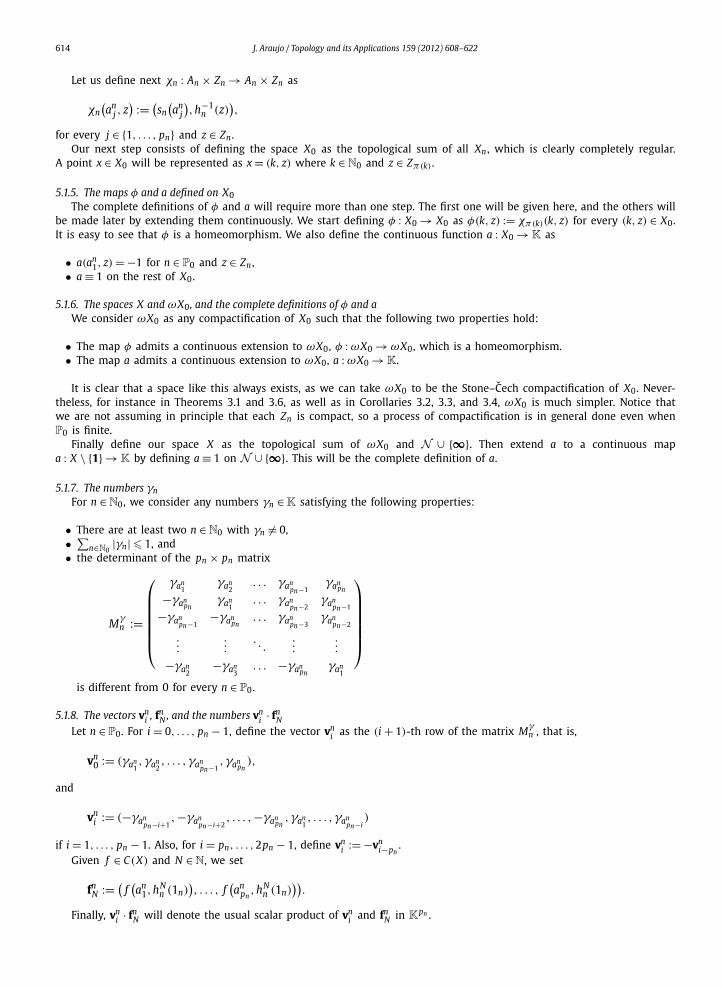
5.1.7. The numbers γn

For n ∈ N0, we consider any numbers γn ∈ K satisfying the following properties:

• There are at least two n ∈ N0 with γn �= 0,• ∑

n∈N0|γn| � 1, and

• the determinant of the pn × pn matrix

Mγn :=

⎛⎜⎜⎜⎜⎜⎜⎝

γan1

γan2

. . . γanpn−1

γanpn

−γanpn

γan1

. . . γanpn−2

γanpn−1−γan

pn−1−γan

pn. . . γan

pn−3γan

pn−2

......

. . ....

...

−γan2

−γan3

. . . −γanpn

γan1

⎞⎟⎟⎟⎟⎟⎟⎠

is different from 0 for every n ∈ P0.

5.1.8. The vectors vni , fn

N , and the numbers vni · fn

N

Let n ∈ P0. For i = 0, . . . , pn − 1, define the vector vni as the (i + 1)-th row of the matrix Mγ

n , that is,

vn0 := (γan

1, γan

2, . . . , γan

pn−1, γan

pn),

and

vni := (−γan

pn−i+1,−γan

pn−i+2, . . . ,−γan

pn, γan

1, . . . , γan

pn−i)

if i = 1, . . . , pn − 1. Also, for i = pn, . . . ,2pn − 1, define vni := −vn

i−pn.

Given f ∈ C(X) and N ∈ N, we set

fnN := (

f(an

1,hNn (1n)

), . . . , f

(an

pn,hN

n (1n)))

.

Finally, vn · fn will denote the usual scalar product of vn and fn in Kpn .
i N i N


5.1.9. The map � and the isometry TWe now define � in the dual space C(X)′ as

�( f ) :=∑n∈P0

( ∑m∈An

γm f (m,1n)

)

for every f ∈ C(X). Obviously ‖�‖ � 1.Finally we introduce the codimension 1 linear isometry T := T [a, φ,�]. In particular we see that, for k ∈ N and z ∈ Zπ(k) ,

(T f )(k, z) := − f (φ(k, z)) if k coincides with aπ(k)1 , and (T f )(k, z) = f (φ(k, z)) otherwise. It is easy to check that T is not an

isometric shift of type II since we deal with at least one pn �= 1 and two γn �= 0.

5.2. The results

In this subsection we follow the notation given in Subsection 5.1.

Lemma 5.1. If f ∈ ⋂∞i=1 T i(C(X)), then f is constant on N ∪ {∞∞∞}. Moreover

f(

N ∪ {∞∞∞}) ≡∞∑

n=1

vn[k mod 2pn] · fn

N ,

where this value is the same for every N ∈ N and k ∈ N ∪ {0}.

Proof. We will give the proof in the case when P0 = N, since the other cases are similar.It is easy to see that, if k = tpn for some t ∈ Z and n ∈ N, then φk(m, z) = (m,h−k

n (z)) whenever m ∈ An and z ∈ Zn . Fromthis we easily deduce the following claim.

Claim 5.2. Let m ∈ An and k = tpn for some t ∈ Z, n ∈ N. We have that, given any z ∈ Zn,

• if t is odd, then (T k f )(m,hkn(z)) = − f (m, z), and

• if t is even, then (T k f )(m,hkn(z)) = f (m, z).

Now, the proof of the next claim is easy, taking into account that f (k) = (T −k+1 f )(1).

Claim 5.3. For every k ∈ N ,

f (k) = �(T −k f

)=

∑n∈P0

( ∑m∈An

γm(T −k f

)(m,1n)

).

Claim 5.4. Let n, N ∈ N, and k ∈ N ∪ {0}. Then∑m∈An

γm(T −k f

)(m,hN−k

n (1n)) = vn

[k mod 2pn] · fnN .

Let us prove Claim 5.4. For simplicity, we denote y := hNn (1n) and wi := f (an

i , y), for i = 1, . . . , pn , that is, fnN =

(w1, . . . , w pn ). Notice first that, for every (m, z) ∈ Xn , f (m, z) = a(m, z)(T −1 f )(χn(m, z)), so taking into account that themaps a and 1/a coincide, we see that (T −1 f )(m, z) = a(χ−1

n (m, z)) f (χ−1n (m, z)). Consequently, if m ∈ An , then(

T −1 f)(

m,h−1n (y)

) = a(χ−1

n

(m,h−1

n (y)))

f(χ−1

n

(m,h−1

n (y)))

,

which means that (T −1 f )(anpn

,h−1n (y)) = − f (an

1, y), and (T −1 f )(ani ,h−1

n (y)) = f (ani+1, y) for i ∈ {1,2, . . . , pn − 1}. It is clear

that in this case

pn∑i=1

γani

(T −1 f

)(an

i ,h−1n (y)

) = −γanpn

w1 + γan1

w2 + · · · + γanpn−1

w pn

= vn · fn .
1 N


Of course a similar process shows that, if k ∈ {2, . . . , pn − 1}, then(T −k f

)(m,h−k

n (y)) = a

(χ−1

n

(m,h−k

n (y)))(

T 1−k f)(

χ−1n

(m,h−k

n (y)))

=(

2∏i=1

a(χ−i

n

(m,h−k

n (y))))(

T 2−k f)(

χ−2n

(m,h−k

n (y)))

...

=(

k∏i=1

a(χ−i

n

(m,h−k

n (y))))

f(χ−k

n

(m,h−k

n (y)))

,

that is,(T −k f

)(an

pn,h−k

n (y)) = −wk,(

T −k f)(

anpn−1,h−k

n (y)) = −wk−1,

...(T −k f

)(an

pn−k+1,h−kn (y)

) = −w1, and(T −k f

)(an

j ,h−kn (y)

) = wk+ j

for j ∈ {1, . . . , pn − k}. As above this implies that∑m∈An

γm(T −k f

)(m,h−k

n (y)) = vn

k · fnN . (5.1)

Next, suppose for instance that k = apn + b, where a is odd and b ∈ {0, . . . , pn − 1}. According to Claim 5.2, we have that(T −apn−b f

)(m,h−apn−b

n (y)) = (

T −apn(T −b f

))(m,h−apn−b

n (y))

= −(T −b f

)(m,h−b

n (y)),

and it is immediate from equality (5.1) that∑m∈An

γm(T −apn−b f

)(m,h−apn−b

n (y)) = −vn

b · fnN = vn

pn+b · fnN .

The case when a is even is similar. This finishes the proof of Claim 5.4.Next fix any ε > 0, and take n0 ∈ N such that

‖ f ‖∞∑

n=n0+1

( ∑m∈An

|γm|)

< ε.

Define, for each k ∈ N,

B(k) :=n0∑

n=1

( ∑m∈An

γm(T −k f

)(m,1n)

).

By Claim 5.3, it is clear that for every k,∣∣ f (k) − B(k)∣∣ < ε. (5.2)

Now make a partition of the set of natural numbers as follows. For i = 0, . . . ,2pn0 − 1, let

Mi := {n ∈ N: n = i mod 2pn0}.Fix any N ∈ N. Since (Zn,hn,1n)n∈P0 is L0-transitive and 2pn0 ∈ L0, then (hN

1 (11), . . . ,hNn0

(1n0 )) is a limit point of

{(hl1(11), . . . ,hl

1(1n0 )): l ∈ Mi} in∏n0

n=1 Zn , for each i = 0, . . . ,2pn0 − 1. Then, taking into account that the map P f :∏n0n=1 Zn → Kp1+···+pn0 sending each (z1, . . . , zn0 ) into

P f (z1, . . . , zn0) := (f(a1, z1

), . . . , f

(a1

p , z1), . . . , f

(an0 , zn0

), . . . , f

(an0

p , zn0

))
1 1 1 n0


is continuous, we deduce that there exists an increasing subsequence (uij) in Mi such that, for each n ∈ {1,2, . . . ,n0} and

each m ∈ An ,

limj→∞

f(m,h

uij

n (1n)) = f

(m,hN

n (1n)).

Consider each of the sequences (uij) given above. By Claim 5.4, it is clear that due to our assumptions on the numbers pn ,

B(ui

j

) =n0∑

n=1

vn[ui

j mod 2pn] · fnui

j

=n0∑

n=1

vn[i mod 2pn] · fn

uij.

Now, using equality (5.2) and taking limits we obtain that, for each i = 0, . . . ,2pn0 − 1,∣∣∣∣∣ f (∞∞∞) −n0∑

n=1

vn[i mod 2pn] · fn

N

∣∣∣∣∣ � ε.

We conclude that, for every k ∈ N ∪ {0} and N ∈ N,

f (∞∞∞) =∞∑

n=1

vn[k mod 2pn] · fn

N .

In particular, the sum∑∞

n=1 vn[k mod 2pn] · fn

N does not depend neither on k nor on N . On the other hand, it is clear byClaims 5.3 and 5.4 that, taking N = k,

f (k) =∞∑

n=1

vn[k mod 2pn] · fn

N

for every k ∈ N , so we deduce that f is constant on N ∪ {∞∞∞}. �Lemma 5.5. The set {χk

n (an1,1n): k ∈ Z} is dense in Xn for each n ∈ P0 .

Proof. First, for n ∈ P0 fixed, (Zn,hn,1n) is transitive by hypothesis, so {χ−kn (an

1,hin(1n)): k ∈ pnN, i = 0, . . . , pn −1} is dense

in {an1} × Zn . Also, since (Zm,hm,1m)m∈P0 is {2pn}-transitive, it is easy to check that, for i = 1, . . . , pn − 1, each point hi

n(1n)

belongs to the closure of {h2 jpnn (1n): j ∈ N}. Taking both facts into account, we see that {χ−k

n (an1,1n): k ∈ pnN} is dense in

{an1} × Zn , and this implies that {χ−k

n (an1,1n): k ∈ N} is dense in Xn . �

Theorem 5.6. T is a shift purely of type I. Also, T is ∞-generated if P0 = N, and it is P0-generated if P0 = {1,2, . . . , P0}.

Proof. We split the proof into two parts.

Case 1. Suppose that P0 = {1}. Recall that we are assuming in this case that p1 �= 1. Let us prove that, if f ∈ ⋂∞l=1 T l(C(X)),

then f = 0. Fix any i = 0, . . . , p1 −1. First we have, by Lemma 5.1 that, given any N ∈ N, v1[i mod 2p1] · f1

N = v1[i+p1 mod 2p1] · f1

N .

Taking into account the definition of v1i , this means that −v1

i · f1N = v1

i · f1N , and consequently the product of the matrix Mγ

1and the vector f1

N is 0. Since Mγ1 is invertible, we conclude that f1

N = 0. Since this happens for every N ∈ N, we conclude bydenseness that f ≡ 0 on ωX0. Finally the value given in Lemma 5.1 for f on N ∪ {∞∞∞} must also be 0, and we are done.

The fact that T is 1-generated follows from Lemma 5.5.

Case 2. Suppose that P0 �= {1}. We just give the proof in the case P0 = N, since the other cases are similar. Let f ∈⋂∞l=1 T l(C(X)) with ‖ f ‖ � 1.Let us prove first that f ≡ 0 on N ∪ {∞∞∞}. By hypothesis we have that if n < i, then pi = 2lpn for some l ∈ N, so taking

into account that vn[k mod 2pn] = −vn

[pn+k mod 2pn] for every k ∈ N ∪ {0}, we deduce that

pi∑vn[k mod 2pn] =

2pn∑vn[k mod 2pn] + · · · +

2lpn∑vn[k mod 2pn] = 0.

k=1 k=1 k=2(l−1)pn+1


This implies that, for every N ∈ N and i ∈ N \ {1},

pi∑k=1

f (k) =pi∑

k=1

( ∞∑n=1

vn[k mod 2pn] · fn

N

)

=pi∑

k=1

(i−1∑n=1

vn[k mod 2pn] · fn

N +∞∑

n=i

vn[k mod 2pn] · fn

N

)

=i−1∑n=1

pi∑k=1

vn[k mod 2pn] · fn

N +pi∑

k=1

∞∑n=i

vn[k mod 2pn] · fn

N

=pi∑

k=1

∞∑n=i

vn[k mod 2pn] · fn

N .

Now, by Claim 5.4, taking into account that f is constant on N ∪ {∞∞∞}, we have that

pi∣∣ f (1)

∣∣ �pi∑

k=1

∞∑n=i

∣∣vn[k mod 2pn] · fn

N

∣∣ � pi

∞∑n=p1+···+pi−1+1

|γn|,

for every i ∈ N \ {1}. Consequently, as i goes to infinity, the term∑∞

n=p1+···+pi−1+1 |γn| goes to 0, and we easily concludethat f (1) = 0, and f ≡ 0 on N ∪ {∞∞∞}.

We deduce then that∑∞


N = 0 for every k ∈ N ∪ {0} and N ∈ N.We must now show that this implies that fn

N = 0 ∈ Kpn . First notice that for n0 ∈ N \ {1} and k ∈ N ∪ {0},∣∣2vn0[k mod 2pn0 ] · fn0

N

∣∣ = ∣∣vn0[k mod 2pn0 ] · fn0

N − vn0[k+pn0 mod 2pn0 ] · fn0

N

∣∣=

∣∣∣∣∣n0∑

n=1

vn[k mod 2pn] · fn

N −n0∑

n=1

vn[k+pn0 mod 2pn] · fn

N

∣∣∣∣∣, (5.3)

and ∣∣∣∣∣2n0−1∑n=1

vn[k mod 2pn] · fn

N

∣∣∣∣∣ =∣∣∣∣∣n0−1∑n=1

vn[k mod 2pn] · fn

N +n0−1∑n=1


N

∣∣∣∣∣=

∣∣∣∣∣n0∑

n=1

vn[k mod 2pn] · fn

N +n0∑

n=1


N

∣∣∣∣∣. (5.4)

Next take any ε > 0 and n1 ∈ N such that∑∞

n=n1+1(∑

m∈An|γm|) < ε . This obviously gives that |∑n1

n=1 vn[k mod 2pn] ·fn

N | < ε

for every k ∈ N ∪ {0} and N ∈ N. Let us prove that |vn[k mod 2pn] · fn

N | < ε for every n � n1. Of course the result is true for thecase when n1 = 1. Next, if we assume that it holds for n1 � l, we can easily prove it for n1 = l + 1 using equalities (5.3)and (5.4).

We deduce that vn[k mod 2pn] · fn

N = 0 for every n, N ∈ N and k ∈ N ∪ {0}. Due to the properties of each matrix Mγn , we

conclude that fnN = 0 and, by denseness, f must be equal to 0, and T is a shift.

Finally, notice that, given a point x ∈ Xn , the set {φk(x): k ∈ Z} is contained in Xn , which implies that T is ∞-generated.Notice also that if P0 �= N, to prove that T is P0-generated we use both the above fact and Lemma 5.5. �Remark 5.1. In the above proof, we borrow some of the ideas of [17, Theorem 3.5], where the sequence (2n) plays afundamental rôle when proving the existence of an isometric shift of type I on C(X), for X = βN + N ∪ {∞∞∞}. On theother hand, we must add that the proof of Lemma 5.1 is valid even if we just assume that the sequence (pn)n∈P0 satisfiesthat each pn+1 is an integer multiple of pn (and pn+1 > pn), instead of being an P0-compatible sequence. Nevertheless, inTheorem 5.6 our requirements on the sequence (pn) are necessary. Let us see it: Suppose that there exist two different pn

(for instance, p1 and p2) which are odd, and that γ1 = γp1+1 �= 0, and γi = 0 for every other i � p1 + p2. Consider thefunction f ∈ C(X) satisfying

• f ({a1i } × Z1) ≡ 1 if i ∈ {1, . . . , pn1 } is odd, and f ({a1

i } × Z1) ≡ −1 if i is even, and

• f ({a2} × Z2) ≡ −1 if i ∈ {1, . . . , pn2 } is odd, and f ({a2} × Z2) ≡ 1 if i is even,
i i


and is equal to 0 in the rest of X . It is easy to check that∑∞


N ≡ 0 for every k ∈ N ∪ {0} and every N ∈ N.Nevertheless we can see that T f = − f , and consequently T is not a shift.

Remark 5.2. Let us see that the condition on (Zn,hn,1n)n∈P0 of being L0-transitive (following the notation given in Sub-section 5.1.3) is not redundant in Theorem 5.6. Consider for instance the case of Z1 consisting of the union of two copiesof a totally transitive set W (with respect to a homeomorphism r and a point w), that is, Z1 := (Z/2Z) × W . It is clearthat the point 11 := (0, w) ∈ (Z/2Z) × W is transitive for the map h1 : Z1 → Z1, defined as h1(a, x) := (a + 1, r(x)) forevery (a, x) ∈ (Z/2Z) × W . Let A1 := {1,2} and X1 := {1,2} × Z1. We may also consider some other sets Xn defined as inSubsection 5.1, although they will play no rôle in what follows. Define finally χ1 : X1 → X1, X , φ and T using the notationgiven in Subsections 5.1.6 and 5.1.9. In particular, for 1 ∈ N , (T f )(1) = γ1 f (1,11) + γ2 f (2,11) for every f ∈ C(X). We havethat T is a codimension 1 linear isometry, but it is not a shift because the function f defined as f ≡ γ1 on {2} × {0} × W ,f ≡ −γ2 on {1} × {0} × W , and f ≡ 0 on the rest of X , satisfies T 2 f = − f .

5.3. Proofs of Theorem 3.1 and Corollary 3.3

Proof of Theorem 3.1. We give the proof in the case P = N, the other cases being similar. We use the notation given inSubsection 5.1, and then apply Theorem 5.6. We consider {a1

1} × Z1, . . . , {a1p1

} × Z1, and call them Y 11 , . . . , Y p1

1 , respectively.

On the other hand, for each n � 2, we consider {an1} × Zn, . . . , {an

pn} × Zn , and call them Y −pn/2

n , . . . , Y pn/2n , respectively.

For each k ∈ Z \ {0}, we define a number Ik ∈ N in the following way. If k = ±1, . . . ,±p2/2, then Ik := 2, and in general,if n � 2 and k = ±(pn/2 + 1), . . . ,±pn+1/2, then Ik := n + 1. Now, for each k ∈ Z \ {0}, we define Y k as the topological sumof all Y k

n (n � Ik), which is locally compact. Then consider its compactification by one point, denoted ∞k .Let X0 := Y 1

1 + · · · + Y p11 + ⋃∞

|k|=1 Y k . It is clear that if we identify ∞k with the number 1/k ∈ R for each k ∈ Z \ {0},and in {0} ∪ {±1/k: k ∈ N} we have the usual topology induced from R, then ωX0 := X0 ∪ {0} ∪ {±1/k: k ∈ N} becomes acompactification of X0.

Next, by Example 4.7 and Remark 4.2, for each n ∈ N, we can find a homeomorphism hn : Zn → Zn , and a point 1n ∈ Zn

such that (Zn,hn,1n) is N-transitive. Finally, Theorem 5.6 provides us a way to construct an isometric shift as we want. �Proof of Corollary 3.3. First it is clear that if s ∈ N, then the process of the proof of Theorem 3.1 can be done in Cs.

On the other hand, since the countable powers of metrizable spaces are also metrizable, so each Zn can be embeddedin [0,1]N (see [13, Theorem 2.3.23]). We can use the famous result that states that �2 is homeomorphic to RN (see [5]) tofinish the proof. �Remark 5.3. It is well known (and easy to see) that the weight of a separable compact space is at most c, and consequentlysuch a space can be homeomorphically embedded in the Tychonoff cube [0,1]c (see [13, Theorem 2.3.23]). Consider nextthe real linear space B := �1(R) of all R-valued maps f on R such that f (x) �= 0 for at most countably many x ∈ R, andsuch that ‖ f ‖1 := ∑

x∈R| f (x)| < +∞. ‖ · ‖1 determines a Banach space structure on B, whose dual B′ can be identified with

the (real) Banach space �∞(R) of all R-valued bounded maps on R endowed with the supremum norm (see [22, p. 137]).We have that the set T := { f ∈ B′: 0 � f (x) � 1 ∀x ∈ R} is a closed subset of B′ in the weak∗-topology; also, it is norm-

bounded in B′ , so by Alaoglu’s Theorem it is compact. On the other hand, it is clear that the canonical map from [0,1]conto T is indeed a homeomorphism, so each separable compact space can be homeomorphically embedded in any openball of B′ (with the weak∗-topology).

6. A method for obtaining examples of composition operators

In this section, we will analyze in particular the case when the weight a ∈ C(X \ {1}) is constantly equal to 1. Themost basic examples of this type of isometric shifts can be constructed for X = βN and X = N ∪ {∞}, and come from theidentifications with respect to the usual shifts defined on the sequence spaces �∞ (of all bounded sequences) and c (of allconvergent sequences), respectively.

A first approach shows that constructions similar to that given in Section 5 (that is, based on the topological sum of acompact space and N ∪ {∞∞∞}) do not yield an isometric shift.

Proposition 6.1. Let X be compact, and suppose that X = X1 + X2 , with X1 �= ∅ and N being a dense subset of X2 . Suppose also thatφ : X \ {1} → X is a homeomorphism (with φ(n + 1) = n for n ∈ N ). Let T : C(X) → C(X) be a codimension 1 linear isometry suchthat (T f )(x) = f (φ(x)) for every f ∈ C(X) and x ∈ X \ {1}. Then T is not an isometric shift.

Proof. Since we are assuming that T is a linear isometry, then there exists � in the dual space C(X)′ , ‖�‖ � 1, such that(T f )(1) = �( f ) for every f ∈ C(X). Take α0 := �(ξX1 ) and α1 := �(ξX2 ), where ξXi denotes the characteristic functionon Xi . If α0 = 0, then define f0 := ξX1 . Otherwise, there exists γ ∈ K such that γα0 + α1 = 1, and define f0 := γ ξX1 + ξX2 .Then it is easy to check that in either case T f0 = f0, so T is not a shift. �


The above proposition gives us a clue on how to proceed in order to find isometric shifts of type I with a = 1. This willbe done next.

6.1. A remark about notation

In this section, we deal with a compact space Y , for which we assume that there exists a homeomorphism χ : Y → Ysuch that the following two properties hold: 1) It is transitive with respect to a point 1Y ∈ Y , that is, the set {χn(1Y ): n ∈ N}is dense in Y . 2) There exists a point 0Y ∈ Y \ {1Y } which is periodic for χ , of prime period N ∈ N.

Spaces satisfying both requirements can be found for instance in Example 3.5. On the one hand, we have all separableinfinite powers of any compact space with more than one point (see Corollary 4.4). On the other hand, related to this,chaotic homeomorphisms (in the Devaney sense, meaning in particular that they are transitive and have a dense set ofperiodic points; see [9]) provide a rich source of examples. It is well known that, for n � 2, every n-dimensional compactmanifold admits a homeomorphism of this kind (as proved in [1]), and indeed the set of all chaotic measure-preservinghomeomorphisms on it is dense in the space of all measure-preserving homeomorphisms (see also [12,4,3]). Finally, asannounced in [2, Remark 1], these results give us a very different example satisfying the above requirements, as is theSierpinski curve.

We denote 00Y := 0Y , . . . , 0N−1

Y := χ N−1(0Y ). Next we take a compactification of N by N points ∞∞∞0, . . . ,∞∞∞N−1. Namely,for k = 0, . . . , N − 1, define Nk := {n ∈ N : n = k mod N}, and consider the one-point compactification Nk ∪ {∞∞∞k} of Nk .

Let X be the union of Y and N ∪ {∞∞∞0, . . . ,∞∞∞N−1}, where each point ∞∞∞k is identified with the point 0kY of Y . From now

on we will just use the notation ∞∞∞k to denote this point both as a member of Y and of N ∪ {∞∞∞0, . . . ,∞∞∞N−1}.Define the map φ : Y → Y as φ := χ−1. Next take any two numbers δ1, δ2 ∈ K \ {0} satisfying |δ1| + |δ2| � 1 and

(δ1 + δ2)N �= 1, and define � : C(X) → K as

�( f ) := δ1 f (1Y ) + δ2 f(χ N(1Y )

)for every f . It is immediate to see that � is linear and continuous, and that ‖�‖ � 1. Finally we define T : C(X) → C(X) asT := T [1, φ,�]. It is clear that T is not an isometric shift of type II since we are assuming that both δi are different from 0.

6.2. The results

Theorem 6.2. Assume that we follow the notation given in Subsection 6.1. Then T is an isometric shift purely of type I.

Proof. Suppose that f ∈ ⋂∞n=1 T n(C(X)) satisfies ‖ f ‖ � 1. It is clear that for every n ∈ N ,

f (n) = (T −n+1 f

)(1)

= δ1(T −n f

)(1Y ) + δ2

(T −n f

)(χ N(1Y )

)= δ1 f

(χn(1Y )

) + δ2 f(χn+N(1Y )

). (6.1)

Let us now see that f (∞∞∞k) = 0 for k = 0, . . . , N − 1. For each k, define Nk := {n ∈ N: n = k mod N}, and Mk :={χn(1Y ): n ∈ Nk}. We know that there exists λ(0) ∈ {0, . . . , N − 1} such that ∞∞∞0 belongs to the closure of Mλ(0) . Takinginto account that χ is transitive and that χ N (∞∞∞0) = ∞∞∞0, we deduce that there exists an increasing sequence (ni) in Nλ(0)

such that both ( f (χni (1Y ))) and (( f ◦ χ N )(χni (1Y ))) converge to f (∞∞∞0). As a consequence, we have by equality (6.1) that

f (∞∞∞λ(0)) = limi→∞

f (ni)

= limi→∞

δ1 f(χni (1Y )

) + δ2 f(χni+N(1Y )

)= (δ1 + δ2) f (∞∞∞0).

In the same way, we see that, if N > 1, then for any k ∈ {1, . . . , N −1}, there exists λ(k) with f (∞∞∞λ(k)) = (δ1 +δ2) f (∞∞∞k), andthat λ(k) can be taken equal to λ(0)+k mod N . Then f (∞∞∞k) = (δ1 + δ2)

N f (∞∞∞k) for every k, which implies that f (∞∞∞k) = 0.Our next step consists of proving that δ1 f (x) + δ2 f (χ N (x)) = 0 for every x ∈ Y . Notice first that limn→∞ f (n) = 0, so by

equality (6.1), limn→∞ δ1 f (χn(1Y )) + δ2 f (χn+N (1Y )) = 0. Now, as above, if x ∈ Y , then there exists an increasing sequence(mi) in N such that ( f (χmi (1Y ))) and ( f (χmi+N (1Y ))) converge to f (x) and f (χ N (x)), respectively. Consequently,

δ1 f (x) + δ2 f(χ N(x)

) = limi→∞ δ1 f

(χmi (1Y )

) + δ2 f(χmi+N(1Y )

) = 0,

as we wanted to see.In particular, the above implies by equality (6.1) that f (n) = 0 for every n ∈ N . It also implies that, for every x ∈ Y ,

f (x) = −(δ2/δ1) f (χ N (x)), so


f (x) = (−1)n(

δ2

δ1

)n

f(χnN(x)

)for every n ∈ N. Obviously, to keep f bounded, we need either that f ≡ 0 on Y or that |δ1| = |δ2|. But remark that in thelatter case | f (x)| = | f (χnN (x))| for every x ∈ Y and every n ∈ N. Now fix k ∈ {0, . . . , N − 1}, and notice that ∞∞∞k belongsto the closure of Mλ(k) . We deduce that | f (∞∞∞k)| = | f (χλ(k)(1Y ))|, and that f (χλ(k)+nN (1Y )) = 0 for every n ∈ N ∪ {0}.A similar process allows us to show that f (χ i+nN (1Y )) = 0 for every i ∈ {0, . . . , N − 1} and n ∈ N ∪ {0}. By denseness, f ≡ 0on Y , as we wanted to prove. �

The proof of the following corollary is now easy.

Corollary 6.3. Let n ∈ N. Let Y0 be a connected and compact space with more than one point, and suppose that φ : Y0 → Y0 is ahomeomorphism having a periodic point, and such that φn is transitive. Then there exist a compact space X and an isometric shiftpurely of type I on C(X) with a ≡ 1, such that X \ N consists exactly of n connected components with more than one point, eachhomeomorphic to Y0 .

7. The case of the Cantor set

Here we use results given in Sections 5 and 6 to prove Theorem 3.6.

Proof of Theorem 3.6. Without loss of generality we assume that (xn) is strictly monotone. Suppose first that L /∈ K. Thenthe result is an immediate consequence of Corollary 3.3 (see also its proof). If we take Zn = K for each n ∈ N, then ωX0 willbe a compact, metrizable and zero-dimensional set without isolated points, which implies that ωX0 is itself homeomorphicto the Cantor set, and we are done.

Suppose next that L ∈ K. It is well known that if Zp is the ring of p-adic integers (p � 2), then there exists a homeo-morphism i : Zp → K. By Corollary 4.5, there are a homeomorphism φ : K → K and points w, M in K such that (K, φ, w)

is totally transitive and φ(M) = M . Let L0 := i−1(L), M0 := i−1(M) ∈ Zp , and define s : Zp → Zp as s(t) := t − L0 + M0 forevery t ∈ Zp . Obviously j := i ◦ s ◦ i−1 is a homeomorphism from K onto itself such that j(L) = M . As in Lemma 4.2, it iseasy to see that (K, j−1 ◦ φ ◦ j, j−1(w)) is totally transitive, and that j−1 ◦ φ ◦ j(L) = L.

Our final step consists of applying Theorem 6.2 (where we identify K with Y and L with 0Y = ∞∞∞), and the proof isfinished. �Remark 7.1. In Theorem 3.6, when L /∈ K, there is no isometric shift with a ≡ 1. This is an immediate consequence ofProposition 6.1.

Acknowledgement

The author would like to thank Professor Francisco Santos for useful conversations.

References

[1] J.M. Aarts, F.G.M. Daalderop, Chaotic homeomorphisms on manifolds, Topology Appl. 96 (1999) 93–96.[2] J.M. Aarts, L.G. Oversteegen, The dynamics of the Sierpinski curve, Proc. Amer. Math. Soc. 120 (1994) 965–968.[3] S. Alpern, V.S. Prasad, Typical Dynamics of Volume Preserving Homeomorphisms, Cambridge University Press, Cambridge, 2000.[4] S. Alpern, V.S. Prasad, Maximally chaotic homeomorphisms of sigma-compact manifolds, Topology Appl. 105 (2000) 103–112.[5] R.D. Anderson, Hilbert space is homeomorphic to the countable infinite product of lines, Bull. Amer. Math. Soc. 72 (1966) 515–519.[6] J. Araujo, On the separability problem for isometric shifts on C(X), J. Funct. Anal. 256 (2009) 1106–1117.[7] J. Araujo, J.J. Font, Codimension 1 linear isometries on function algebras, Proc. Amer. Math. Soc. 127 (1999) 2273–2281.[8] J. Araujo, J.J. Font, Isometric shifts and metric spaces, Monatshefte Math. 134 (2001) 1–8.[9] J. Banks, J. Brooks, G. Cairns, G. Davis, P. Stacey, On Devaney’s definition of chaos, Amer. Math. Monthly 99 (1992) 332–334.

[10] L.-S. Chen, J.-S. Jeang, N.-C. Wong, Disjointness preserving shifts on C0(X), J. Math. Anal. Appl. 325 (2007) 400–421.[11] R.M. Crownover, Commutants of shifts on Banach spaces, Michigan Math. J. 19 (1972) 233–247.[12] F. Daalderop, R. Fokkink, Chaotic homeomorphisms are generic, Topology Appl. 102 (2000) 297–302.[13] R. Engelking, General Topology, Heldermann Verlag, Berlin, 1989.[14] F.O. Farid, K. Varadajaran, Isometric shift operators on C(X), Can. J. Math. 46 (1994) 532–542.[15] J.J. Font, Isometries on function algebras with finite codimensional range, Manuscripta Math. 100 (1999) 13–21.[16] A. Gutek, D. Hart, J. Jamison, M. Rajagopalan, Shift operators on Banach spaces, J. Funct. Anal. 101 (1991) 97–119.[17] A. Gutek, J. Norden, Type 1 shifts on C(X), Topology Appl. 114 (2001) 73–89.[18] R. Haydon, Isometric shifts on C(K ), J. Funct. Anal. 135 (1996) 157–162.[19] J.R. Holub, On shift operators, Canad. Math. Bull. 31 (1988) 85–94.[20] K. Izuchi, Douglas algebras which admit codimension 1 linear isometries, Proc. Amer. Math. Soc. 129 (2001) 2069–2074.[21] J.-S. Jeang, N.-C. Wong, Isometric shifts on C0(X), J. Math. Anal. Appl. 274 (2002) 772–787.[22] G. Köthe, Topological Vector Spaces I, Springer Verlag, Berlin, 1969.[23] J.C. Oxtoby, Measure and Category, Springer Verlag, New York, 1971.[24] M. Rajagopalan, T.M. Rassias, K. Sundaresan, Generalized backward shifts on Banach spaces C(X, E), Bull. Sci. Math. 124 (2000) 685–693.


[25] M. Rajagopalan, K. Sundaresan, Backward shifts on Banach spaces C(X), J. Math. Anal. Appl. 202 (1996) 485–491.[26] M. Rajagopalan, K. Sundaresan, An account of shift operators, J. Anal. 8 (2000) 1–18.[27] M. Rajagopalan, K. Sundaresan, Generalized shifts on Banach spaces of continuous functions, J. Anal. 10 (2002) 5–15.[28] T.M. Rassias, K. Sundaresan, Generalized backward shifts on Banach spaces, J. Math. Anal. Appl. 260 (2001) 36–45.[29] J. de Vries, Elements of Topological Dynamics, Kluwer Academic Publishers, Dordrecht, 1993.

Documents

Examples of isometric shifts on