Examples solving an ODE using finite elements method.Mathematica and Matlab implementation and animation

Nasser M. Abbasi

Sept 28,2006 page compiled on August 19, 2015 at 10:35am

1 Introduction

This is a basic review of Finite Elements Methods from Mathematical point of view with examples ofhow it can be used to numerically solve first and second order ODE’s. Currently I show how to use FEMto solve first and second order ODE. I am also working on a detailed derivation and implementationusing FEM to solve the 2D Poisson’s equation but this work is not yet completed.

FEM is a numerical method for solving differential equations (ordinary or partial). It can also beused to solve non-linear differential equations but I have not yet studied how this is done. FEM is amore versatile numerical method than the finite difference methods for solving differential equations as itsupports more easily different types of geometry and boundary conditions, in addition the solution of thedifferential equation found using FEM can be used at any point in the domain and not just on the gridpoints as the case is with finite difference methods. On the other hand FEM is more mathematicallycomplex method, and its implementation is not as straight forward as with finite difference methods.

Considering only ordinary differential equations with constant coefficients over the x domain (realline).

ady

dx+ b y (x ) = f (x )

ady

dx+ b y (x ) − f (x ) = 0

defined over 0 ≤ x ≤ 1 with the boundary condition y (0) = y0. In the above, only when y (x ) is the exactsolution, call it ye (x ) , do we have the above identity to be true.

In other words, only when y = ye we can write that adyedx + b ye (x ) − f (x ) = 0. Such a differential

equations can be represented as an operator L

L := (y,x ) → ady

dx+ by (x ) − f (x ) (1)

If we know the exact solution, call it ye (x ) then we write

L (ye ,x ) → adyedx+ bye (x ) − f (x )

→ 0

FEM is based on the weighted residual methods (WRM) where we assume that the solution of andifferential equation is the sum of weighted basis functions represented by the symbol ϕi in here. This is

1

in essence is similar to Fourier series, where we represent a function as a weighted sums of series madeup of the basis functions which happened to be in that case the sin and cosine functions.

So the first step in solving the differential equation is to assume that the solution, called y (x ) , canbe written as

y (x ) =N∑j=1

qj ϕj (x )

Where qj are unknown coefficients (the weights) to be determined. Hence the main computationalpart of FEM will be focused on determining these coefficients.

When we substitute this assumed solution in the original ODE such as shown in the above example,equation (1) now becomes

L (y,x ) = ady

dx+ by (x ) − f (x )

= R (x )

Where R (x ) is called the differential equation residual, which is a function over x and in general willnot be zero due to the approximate nature of our assumed solution. Our goal is to to determine thecoefficients qj which will make R (x ) the minimum over the domain of the solution.

The optimal case is for R (x ) to be zero over the domain. One method to be able to achieve this is byforcing R (x ) to meet the following requirement∫

Ω

R (x ) vi (x ) dx = 0

for all possible sets of function vi (x ) which are also defined over the same domain. The functionsvi (x ) are linearly independent from each others. If we can make R (x ) satisfy the above for each one ofthese functions, then this implies that R (x ) is zero. And the solution y (x ) will be as close as possibleto the exact solution. We will find out in FEM that the more elements we use, the closer to the exactsolution we get. This property of convergence when it comes to FEM is important, but not analyzedhere.

Each one of these functions vi (x ) is called a test function (or a weight function), hence the name ofthis method.

In the galerkin method of FEM, the test functions are chosen from the same class of functions as thetrial functions as will be illustrated below.

By making R (x ) satisfy the above integral equation (called the weak form of the original differentialequation) for N number of test functions, where N is the number of the unknown coefficients qi , then weobtain a set of N algebraic equations, which we can solve for qi .

The above is the basic outline of all methods based on the weighted residual methods. The choiceof the trial basis functions, and the choice of the test functions, determine the method used. Differentnumerical schemes use different types of trial and test functions.

In the above, the assumed solution y (x ) is made up of a series of trial functions (the basis). Thissolution is assumed to be valid over the whole domain. This is called a global trial function. In methodssuch as Finite Elements and Finite volume, the domain itself is descritized, and the assumed solution ismade up of a series of solutions, each of which is defined over each element resulting from the discretizationprocess.

In addition, in FEM, the unknown coefficients, called qi above, have a physical meaning, they are takenas the solution values at each node. The trial functions themselves are generated by using polynomial

2

interpolation between the nodal values. The polynomial can be linear, quadratic or cubic polynomialor higher order. Lagrangian interpolation method is normally used for this step. The order of thepolynomial is determined by the number of unknowns at the nodes. For example, if our goal is todetermine the displacement at the nodes, then we have 2 unknowns, one at each end of the element.Hence a linear interpolation will be sufficient in this case, since a linear polynomial a0 + a1x contain2 unknowns, the a1 and a0. If in addition to the displacement, we wish to also solve for the rotationat each end of the element, hence we have a total of 4 unknowns, 2 at each end of the element, whichare the displacement and the rotation. Hence the minimum interpolating polynomial needed will be acubic polynomial a0 + a1x + a2x + a3x . In the examples below, we assume that we are only solving fordisplacement, hence a linear polynomial will be sufficient.

At first, we will work with global trial functions to illustrate how to use weighted residual method.

2 Weighted Residual method. Global trial functions.

The best way to learn how to use WRM is by working over and programming some examples.We analyze the solution in terms of errors and the effect of changing N on the result.

2.1 First example. First order ODE

Given the following ODEdy

dx− y (x ) = 0

defined over 0 ≤ x ≤ 1 with the boundary condition y (0) = 1, we wish to solve this numerically using theWRM. This ODE has an exact solution of y = ex .

The solution using WRM will always follow these steps.STEP 1Assume a solution that is valid over the domain 0 ≤ x ≤ 1 to be a series solution of trial (basis)

functions. We start by selecting a trial functions. The assumed solution takes the form of

y (x ) = y0 +N∑j=1

qj ϕj (x )

Where ϕj (x ) is the trial function which we have to choose, and qj are the N unknown coefficients tobe determined subject to a condition which will be shown below. y0 is the assumed solution which needsto be valid only at the boundary conditions. Hence in this example, since we are given that the solutionmust be 1 at the initial condition x = 0, then y0 = 1 will satisfy this boundary condition. Hence our trialsolution is

y = 1 +N∑j=1

qj ϕj (x )

STEP 2Now decide on what trial function ϕ (x ) to use. For this example, we can select the trial functions

to be polynomials in x or trigonometric functions. Let use choose a polynomial ϕj (x ) = x j , hence ourassumed solution becomes

y = 1 +N∑j=1

qj xj (1)

3

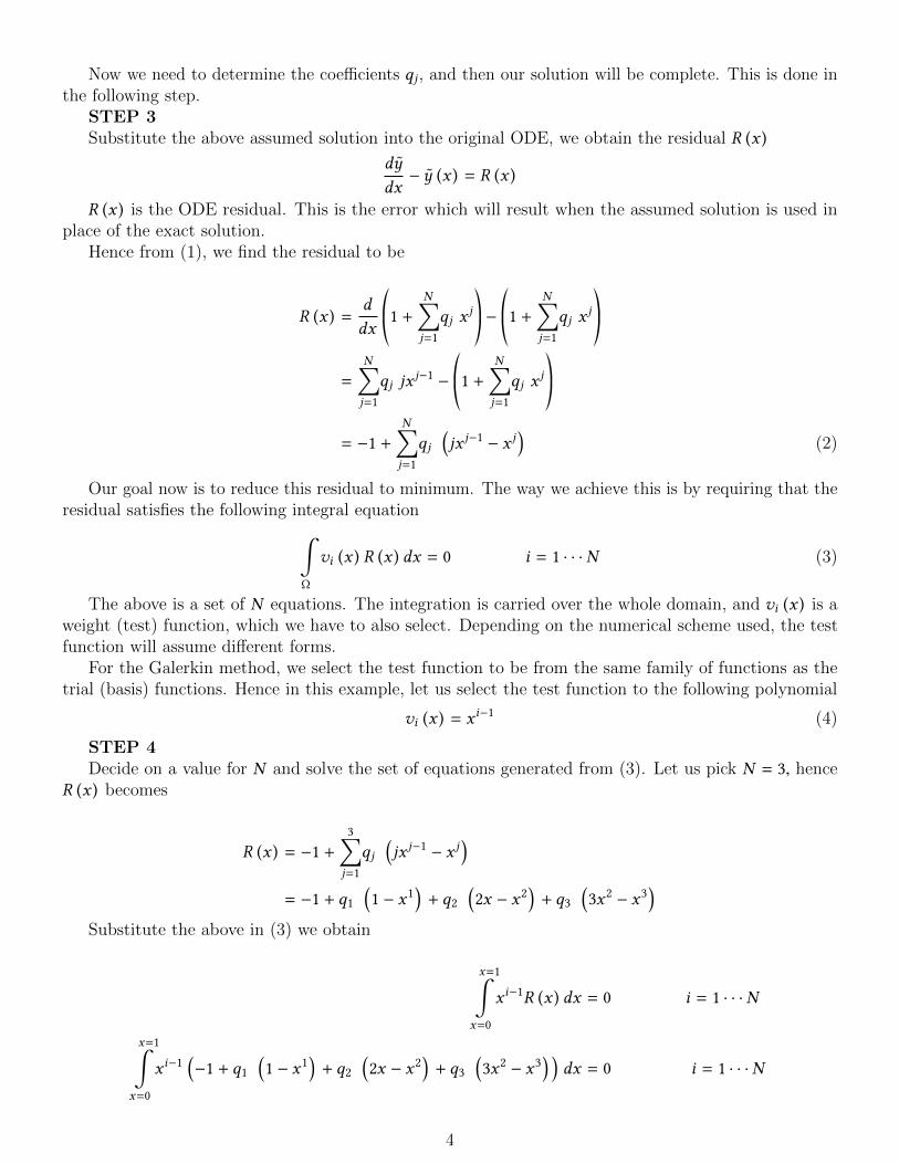
Now we need to determine the coefficients qj , and then our solution will be complete. This is done inthe following step.

STEP 3Substitute the above assumed solution into the original ODE, we obtain the residual R (x )

dy

dx− y (x ) = R (x )

R (x ) is the ODE residual. This is the error which will result when the assumed solution is used inplace of the exact solution.

Hence from (1), we find the residual to be

R (x ) =d

dx*.,1 +

N∑j=1

qj xj+/-−

*.,1 +

N∑j=1

qj xj+/-

=

N∑j=1

qj jxj−1 −

*.,1 +

N∑j=1

qj xj+/-

= −1 +N∑j=1

qj(jx j−1 − x j

)(2)

Our goal now is to reduce this residual to minimum. The way we achieve this is by requiring that theresidual satisfies the following integral equation∫

Ω

vi (x ) R (x ) dx = 0 i = 1 · · ·N (3)

The above is a set of N equations. The integration is carried over the whole domain, and vi (x ) is aweight (test) function, which we have to also select. Depending on the numerical scheme used, the testfunction will assume different forms.

For the Galerkin method, we select the test function to be from the same family of functions as thetrial (basis) functions. Hence in this example, let us select the test function to the following polynomial

vi (x ) = xi−1 (4)

STEP 4Decide on a value for N and solve the set of equations generated from (3). Let us pick N = 3, hence

R (x ) becomes

R (x ) = −1 +3∑j=1

qj(jx j−1 − x j

)= −1 + q1

(1 − x1

)+ q2

(2x − x2

)+ q3

(3x2 − x3

)Substitute the above in (3) we obtain

x=1∫x=0

xi−1R (x ) dx = 0 i = 1 · · ·N

x=1∫x=0

xi−1(−1 + q1

(1 − x1

)+ q2

(2x − x2

)+ q3

(3x2 − x3

) )dx = 0 i = 1 · · ·N

4

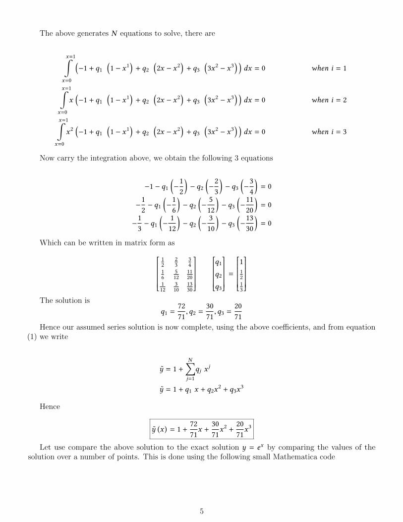
The above generates N equations to solve, there are

x=1∫x=0

(−1 + q1

(1 − x1

)+ q2

(2x − x2

)+ q3

(3x2 − x3

) )dx = 0 when i = 1

x=1∫x=0

x(−1 + q1

(1 − x1

)+ q2

(2x − x2

)+ q3

(3x2 − x3

) )dx = 0 when i = 2

x=1∫x=0

x2(−1 + q1

(1 − x1

)+ q2

(2x − x2

)+ q3

(3x2 − x3

) )dx = 0 when i = 3

Now carry the integration above, we obtain the following 3 equations

−1 − q1(−12

)− q2

(−23

)− q3

(−34

)= 0

−12− q1

(−16

)− q2

(−512

)− q3

(−1120

)= 0

−13− q1

(−112

)− q2

(−310

)− q3

(−1330

)= 0

Which can be written in matrix form as

12

23

34

16

512

1120

112

310

1330

q1

q2

q3

=

11213

The solution is

q1 =7271,q2 =

3071,q3 =

2071

Hence our assumed series solution is now complete, using the above coefficients, and from equation(1) we write

y = 1 +N∑j=1

qj xj

y = 1 + q1 x + q2x2 + q3x

3

Hence

y (x ) = 1 +7271

x +3071

x2 +2071

x3

Let use compare the above solution to the exact solution y = ex by comparing the values of thesolution over a number of points. This is done using the following small Mathematica code

5

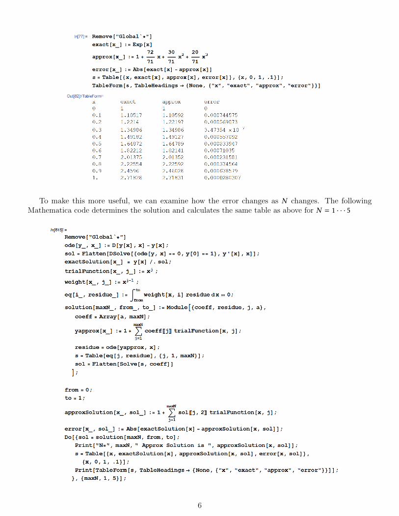
To make this more useful, we can examine how the error changes as N changes. The followingMathematica code determines the solution and calculates the same table as above for N = 1 · · · 5

6

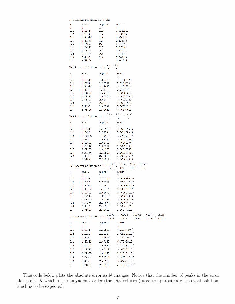
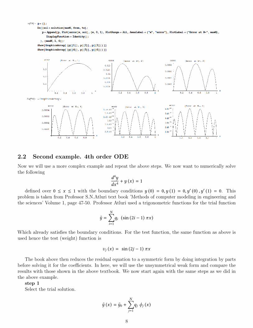
This code below plots the absolute error as N changes. Notice that the number of peaks in the errorplot is also N which is the polynomial order (the trial solution) used to approximate the exact solution,which is to be expected.

7

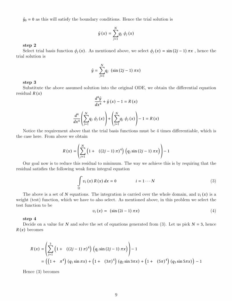
2.2 Second example. 4th order ODE

Now we will use a more complex example and repeat the above steps. We now want to numerically solvethe following

d4y

dx4+ y (x ) = 1

defined over 0 ≤ x ≤ 1 with the boundary conditions y (0) = 0,y (1) = 0,y′ (0) ,y′ (1) = 0. Thisproblem is taken from Professor S.N.Atluri text book ’Methods of computer modeling in engineering andthe sciences’ Volume 1, page 47-50. Professor Atluri used a trigonometric functions for the trial function

y =N∑i=1

qi (sin (2i − 1) πx )

Which already satisfies the boundary conditions. For the test function, the same function as above isused hence the test (weight) function is

vj (x ) = sin (2j − 1) πx

The book above then reduces the residual equation to a symmetric form by doing integration by partsbefore solving it for the coefficients. In here, we will use the unsymmetrical weak form and compare theresults with those shown in the above textbook. We now start again with the same steps as we did inthe above example.

step 1Select the trial solution.

y (x ) = y0 +N∑j=1

qj ϕj (x )

8

y0 = 0 as this will satisfy the boundary conditions. Hence the trial solution is

y (x ) =N∑j=1

qj ϕj (x )

step 2Select trial basis function ϕj (x ) . As mentioned above, we select ϕj (x ) = sin (2j − 1) πx , hence the

trial solution is

y =N∑j=1

qj (sin (2j − 1) πx )

step 3Substitute the above assumed solution into the original ODE, we obtain the differential equation

residual R (x )d4y

dx4+ y (x ) − 1 = R (x )

d4

dx4*.,

N∑j=1

qj ϕj (x )+/-+

*.,

N∑j=1

qj ϕj (x )+/-− 1 = R (x )

Notice the requirement above that the trial basis functions must be 4 times differentiable, which isthe case here. From above we obtain

R (x ) = *.,

N∑j=1

(1 + ( (2j − 1) π )4

) (qj sin (2j − 1) πx

) +/-− 1

Our goal now is to reduce this residual to minimum. The way we achieve this is by requiring that theresidual satisfies the following weak form integral equation∫

Ω

vi (x ) R (x ) dx = 0 i = 1 · · ·N (3)

The above is a set of N equations. The integration is carried over the whole domain, and vi (x ) is aweight (test) function, which we have to also select. As mentioned above, in this problem we select thetest function to be

vi (x ) = (sin (2i − 1) πx ) (4)

step 4Decide on a value for N and solve the set of equations generated from (3). Let us pick N = 3, hence

R (x ) becomes

R (x ) = *.,

3∑j=1

(1 + ( (2j − 1) π )4

) (qj sin (2j − 1) πx

) +/-− 1

=( (1 + π 4

)(q1 sinπx ) +

(1 + (3π )4

)(q2 sin 3πx ) +

(1 + (5π )4

)(q3 sin 5πx )

)− 1

Hence (3) becomes

9

∫Ω

vi (x ) R (x ) dx = 0 i = 1 · · ·N

1∫0

(sin (2i − 1) πx ) R (x ) dx = 0 i = 1 · · ·N

1∫0

(sin (2i − 1) πx ) ( (

1 + π 4)(q1 sinπx ) +

(1 + (3π )4

)(q2 sin 3πx ) +

(1 + (5π )4

)(q3 sin 5πx )

)− 1

dx = 0 i = 1 · · ·N

The above generates N equations to solve for the coefficients qi

1∫0

(sinπx ) ( (

1 + π 4)(q1 sinπx ) +

(1 + (3π )4

)(q2 sin 3πx ) +

(1 + (5π )4

)(q3 sin 5πx )

)− 1

dx = 0 i = 1

1∫0

(sin 3πx ) ( (

1 + π 4)(q1 sinπx ) +

(1 + (3π )4

)(q2 sin 3πx ) +

(1 + (5π )4

)(q3 sin 5πx )

)− 1

dx = 0 i = 2

1∫0

(sin 5πx ) ( (

1 + π 4)(q1 sinπx ) +

(1 + (3π )4

)(q2 sin 3πx ) +

(1 + (5π )4

)(q3 sin 5πx )

)− 1

dx = 0 i = 3

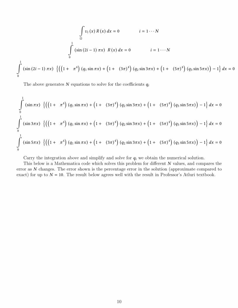
Carry the integration above and simplify and solve for qi we obtain the numerical solution.This below is a Mathematica code which solves this problem for different N values, and compares the

error as N changes. The error shown is the percentage error in the solution (approximate compared toexact) for up to N = 10. The result below agrees well with the result in Professor’s Atluri textbook.

10

3 Finite element method

3.1 Example one. First order ODE, linear interpolation

Let us first summarize what we have discussed so far. Given a differential equation defined over domain

Ω, we assume its solution to be of the form u (x ) =N∑j=1

qj ϕj (x ) .

The function ϕj (x ) is called the jth basis function. qj ϕj (x ) is called a trial function.The function ϕj (x ) is made up of functions called the shape functions Nk as they are normally called

in structural mechanics books.qj are the unknown coefficients which are determined by solving N set of equations generated by

11

setting N integrals of the form

∫Ω

R (x ) vi (x ) dx to zero. Where R (x ) is the differential equation residual

and vi (x ) is the ith weight function where i = 1 · · ·N . In all what follows N is the taken as the numberof nodes.

In FEM, we also carry the same basic process as was described above, the differences are the following:We divide the domain itself into a number of elements. Next, the ϕj (x ) function is found by assuming

the solution to be an interpolation between the nodes of the element. The solution values at the nodesare the qi and are of course unknown except at the boundaries as given by the problem.

We start by deciding on what interpolation between the nodes to use. We will use polynomialinterpolation. Then qjϕj (x ) will become the interpolation function.

In addition, the coefficients qj represent the solution at the node j. These are the unknowns, whichwe will solve for by solving the weak form integral equation as many times as there are unknowns tosolve for.

By solving for the nodal values, we can then use the interpolating function again to find the solutionat any point between the nodes.

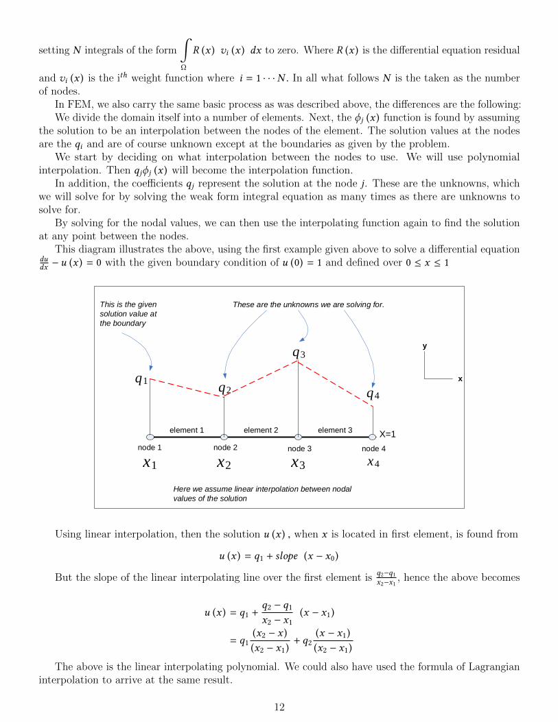
This diagram illustrates the above, using the first example given above to solve a differential equationdudx − u (x ) = 0 with the given boundary condition of u (0) = 1 and defined over 0 ≤ x ≤ 1

x1 x2 x3

X=1

This is the given

solution value at

the boundary

These are the unknowns we are solving for.

Here we assume linear interpolation between nodal

values of the solution

x

y

node 1 node 2 node 3 node 4

element 1 element 2 element 3

q1q2

q3

x4

q4

Using linear interpolation, then the solution u (x ) , when x is located in first element, is found from

u (x ) = q1 + slope (x − x0)

But the slope of the linear interpolating line over the first element isq2−q1x2−x1

, hence the above becomes

u (x ) = q1 +q2 − q1x2 − x1

(x − x1)

= q1(x2 − x )

(x2 − x1)+ q2

(x − x1)

(x2 − x1)

The above is the linear interpolating polynomial. We could also have used the formula of Lagrangianinterpolation to arrive at the same result.

12

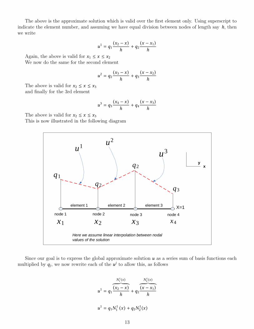
The above is the approximate solution which is valid over the first element only. Using superscript toindicate the element number, and assuming we have equal division between nodes of length say h, thenwe write

u1 = q1(x2 − x )

h+ q2

(x − x1)

h

Again, the above is valid for x1 ≤ x ≤ x2We now do the same for the second element

u2 = q2(x3 − x )

h+ q3

(x − x2)

h

The above is valid for x2 ≤ x ≤ x3and finally for the 3rd element

u3 = q3(x4 − x )

h+ q4

(x − x3)

h

The above is valid for x2 ≤ x ≤ x3This is now illustrated in the following diagram

q2

q3

u1u2

u3

x1 x2 x3

X=1

Here we assume linear interpolation between nodal

values of the solution

xy

node 1 node 2 node 3 node 4

element 1 element 2 element 3

q2

x4

q1

Since our goal is to express the global approximate solution u as a series sum of basis functions eachmultiplied by qj , we now rewrite each of the u j to allow this, as follows

u1 = q1

N 11 (x )︷ ︸︸ ︷

(x2 − x )

h+ q2

N 12 (x )︷ ︸︸ ︷

(x − x1)

h

u1 = q1N11 (x ) + q2N

12 (x )

13

Again, the above is valid for x1 ≤ x ≤ x2. Notice the use of the following notation: Since each elementwill have defined on it 2 shape functions, N1 (x ) and N2 (x ) , then we use a superscript to indicate theelement number. Hence for element 1, we will write N 1

1 (x ) and N 12 (x ).

We now do the same for the second element

u2 = q2

N 21 (x )︷ ︸︸ ︷

(x3 − x )

h+ q3

N 22 (x )︷ ︸︸ ︷

(x − x2)

hu2 = q2N

21 (x ) + q3N

22 (x )

The above is valid for x2 ≤ x ≤ x3and finally for the 3rd element

u3 = q3

N 31 (x )︷ ︸︸ ︷

(x4 − x )

h+ q4

N 32 (x )︷ ︸︸ ︷

(x − x3)

hu3 = q3N

31 + q4N

32

The above is valid for x2 ≤ x ≤ x3The global trial function is

u (x ) = u1 + u2 + u3

=(q1N

11 + q2N

12

)+

(q2N

21 + q3N

22

)+

(q3N

31 + q4N

32

)= q1N

11 + q2

(N 12 + N

21

)+ q3

(N 22 + N

31

)+ q4

(N 32

)The shape function for node 1 is

ϕ1 = N 11

=x2 − x

h

And the shape function for node 2 is

ϕ2 = N 12 + N

21

=(x − x1)

h+

(x3 − x )

h

The shape function for node 3 is

ϕ3 = N 22 + N

31

=(x − x2)

h+

(x4 − x )

h

The shape function for the last node is

ϕ4 = N 32

=x − x3h

14

Hence for the first node, the shape function is ϕ1 =(x2−x )

h , for the last node ϕn =(x−xn−1)

h and theshape function for any internal node is

ϕj =x − xj−1

h+xj+1 − x

h

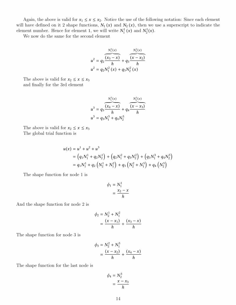
The approximate solution is

u (x ) =Number Nodes∑

i=1

qiϕi

This completes the first part, which was to express the global approximate solution as sum of basisfunctions, each multiplied by an unknowns q coefficients.

The diagram below illustrates the above.

x1 x2 x3

X=1

x

y

node 1 node 2 node 3 node 4

element 1 element 2 element 3

q1q2

q3

u1 q1N11x q2N2

1x

u2 q2N12x q3N2

2x

u3 q3N13 q4N2

3

x4

q4

The diagram below illustrates the numbering used.

15

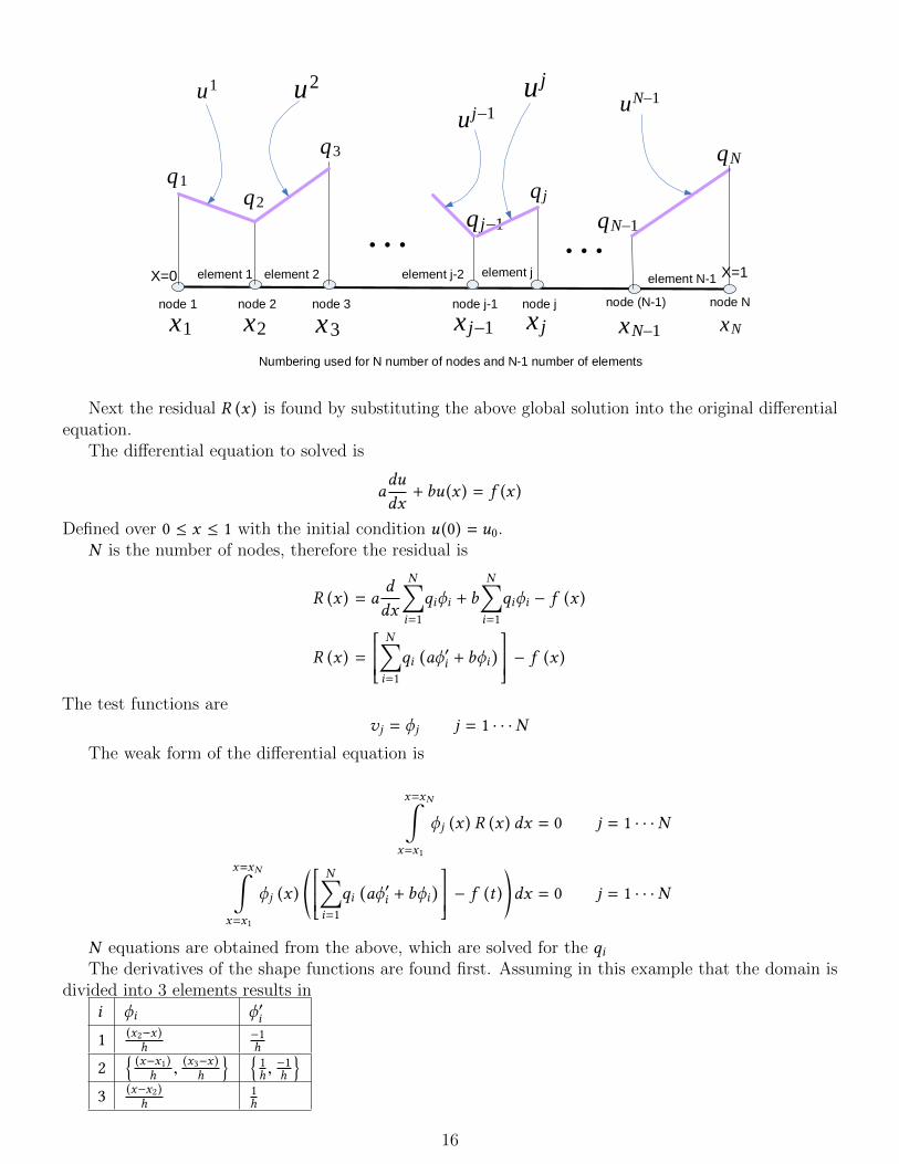
x1 x2

X=1

node 1 node 2 node 3 node j-1

element 1 element 2 element j-2

q1

q2

x j1

node j

x j

element j

xN1

element N-1

q j1

q j

qN1

qN

u1 u2

u j1

u j

uN1

node (N-1) node N

X=0

q3

x3 xN

Numbering used for N number of nodes and N-1 number of elements

Next the residual R (x ) is found by substituting the above global solution into the original differentialequation.

The differential equation to solved is

adu

dx+ bu (x ) = f (x )

Defined over 0 ≤ x ≤ 1 with the initial condition u (0) = u0.N is the number of nodes, therefore the residual is

R (x ) = ad

dx

N∑i=1

qiϕi + bN∑i=1

qiϕi − f (x )

R (x ) =

N∑i=1

qi(aϕ′i + bϕi

) − f (x )

The test functions arevj = ϕj j = 1 · · ·N

The weak form of the differential equation is

x=xN∫x=x1

ϕj (x ) R (x ) dx = 0 j = 1 · · ·N

x=xN∫x=x1

ϕj (x ) *,

N∑i=1

qi(aϕ′i + bϕi

) − f (t )+

-dx = 0 j = 1 · · ·N

N equations are obtained from the above, which are solved for the qiThe derivatives of the shape functions are found first. Assuming in this example that the domain is

divided into 3 elements results ini ϕi ϕ′i

1 (x2−x )h

−1h

2(x−x1)

h , (x3−x )h

1h ,−1h

3 (x−x2)h

1h

16

In general, if there are N nodes, then for the first node

ϕ1 =(x2 − x )

h

ϕ′1 =−1h

And for the last node

ϕN =(x − xN−1)

h

ϕ′N =1h

And for any node in the middle

ϕi =(x − xi−1)

h

ϕ′i =1h

for xi−1 ≤ x ≤ xi and

ϕi =(xi+1 − x )

h

ϕ′i =−1h

for xi ≤ x ≤ xi+1.Looking back at the weak form integral above, it is evaluated as follows

x=xN∫x=x1

ϕj*,

N∑i=1

qi(aϕ′i + bϕi

) − f (x )+

-dx = 0 j = 1 · · ·N

For the first node only, j = 1, the following results

x=xN∫x=x1

ϕ1 *,

N∑i=1

qi(aϕ′i + bϕi

) − f (x )+

-dx = 0

Since ϕ1 is none zero only over x1 ≤ x ≤ x2, and given that ϕ1 =x2−xh ,ϕ

′1 =

−1h ,ϕ2 =

(x−x1)h due to the

range of integration limits, and that ϕ′2 =1h , then the above can simplified to give

x=x2∫x=x1

ϕ1( [q1

(aϕ′1 + bϕ1

)+ q2

(aϕ′2 + bϕ2

) ]− f (x )

)dx = 0

x=x2∫x=x1

(x2 − x )

h

( [q1

(−a

h+ b

(x2 − x )

h

)+ q2

(a1h+ b

(x − x1)

h

) ]− f (x )

)dx = 0

17

The above simplifies further to

−q1

((3a + 2b (x1 − x2) ) (x1 − x2)

2

6h2

)− q2

(−3a + b (x1 − x2) ) (x1 − x2)2

6h2−

x=x2∫x=x1

ϕ1 f (x ) = 0

−q1

((3a + 2b (x1 − x2) ) (x1 − x2)

2

6h2

)− q2

(−3a + b (x1 − x2) ) (x1 − x2)2

6h2−1h

x=x2∫x=x1

(x2 − x ) f (x ) = 0

Since x2 − x1 = h and x1 − x2 = −h the above reduces

−q1

((3a − 2bh) h2

6h2

)− q2

(−3a − bh) h2

6h2−1h

x=x2∫x=x1

(x2 − x ) f (x ) = 0

q1

(2bh − 3a

6

)+ q2

(bh + 3a

6

)−1h

x=x2∫x=x1

(x2 − x ) f (x ) = 0

The above equation gives the first row in the global stiffness matrix for any first order linear ODE ofthe form adu

dx +bu (x ) = f (x ). The above shows that numerical integration is only needed to be performed

on the term

x=x2∫x=x1

(x2 − x ) f (x )

Next the last equation is found, which will be the last row of the stiffness matrix. For the last nodeonly j = N the following results

x=xN∫x=xN−1

ϕN*,

N∑i=1

qi(aϕ′i + bϕi

) − f (x )+

-dx = 0

Since ϕN domain of influence is xN−1 ≤ x ≤ xN , the above simplifies to

x=xN∫x=xN−1

ϕN

( [qN−1

(aϕ′N−1 + bϕN−1

)+ qN

(aϕ′N + bϕN

) ]− f (x )

)dx = 0

Since ϕN−1 =(xN−x )

h ,ϕ′N−1 =−1h ,ϕN =

x−xN−1h ,ϕ′N =

1h the above becomes

x=xN∫x=xN−1

x − xN−1h

( [qN−1

(−a

h+ b

(xN − x )

h

)+ qN

(a1h+ b

x − xN−1h

) ]− f (x )

)dx = 0

Which simplifies to

−qN−1(3a + b (xN−1 − xN ) ) (xN−1 − xN )

2

6h2− qN

(−3a + 2b (xN−1 − xN ) ) (xN−1 − xN )2

6h2−

1h

x=xN∫x=xN−1

(x − xN−1) f (x ) dx = 0

Letting xN−1 − xN = −h in the above becomes

18

qN−1

(bh − 3a

6

)+ qN

(3a + 2bh)6

−1h

x=xN∫x=xN−1

(x − xN−1) f (x ) = 0

Hence the last line of the stiffness matrix can be determined directly except for the term under theintegral which needs to be evaluated using numerical integration.

Now the equation that represents any internal node is found. This will be any row in the globalstiffness matrix between the first and the last row.

For any j other than 1 or N the following results

x=x j∫x=x j−1

ϕj*,

N∑i=1

qi(aϕ′i + bϕi

) − f (x )+

-dx +

x=x j+1∫x=x j

ϕj*,

N∑i=1

qi(aϕ′i + bϕi

) − f (x )+

-dx = 0

Where the integral was broken into two parts to handle the domain of influence of the shape functions.

x=x j∫x=x j−1

ϕj

(qj−1

(aϕ′j−1 + bϕj−1

)+ qj

(aϕ′j + bϕj

)− f (x )

)dx+

x=x j+1∫x=x j

ϕj

(qj

(aϕ′j + bϕj

)+ qj+1

(aϕ′j+1 + bϕj+1

)− f (x )

)dx = 0

For xj−1 ≤ x ≤ xj , ϕj =x−x j−1

h ,ϕ′j =1h ,ϕj−1 =

x j−xh ,ϕ

′j−1 =

−1h

For xj ≤ x ≤ xj+1, ϕj =x j+1−x

h ,ϕ′j =−1h ,ϕj+1 =

x−x jh ,ϕ

′j+1 =

1h

Hence the weak form integral can be written as

x=x j∫x=x j−1

x − xj−1

h

(qj−1

(−a

h+ b

xj − x

h

)+ qj

(ah+ b

x − xj−1

h

)− f (x )

)dx+

x=x j+1∫x=x j

xj+1 − x

h

(qj

(−a

h+ b

xj+1 − x

h

)+ qj+1

(ah+ b

x − xj

h

)− f (x )

)dx = 0

Which simplifies to

qj−1*.,

(−3a − b

(x j−1 − x j

) ) (x j−1 − x j

) 26h2

+/-+ qj

( (3a − 2b

(x j−1 − x j

) ) (x j−1 − x j

) 2)6h2

−1h

x=x j∫x=x j−1

(x − x j−1

)f (x ) dx+

qj*.,

(−3a − 2b

(x j − x j+1

) ) (x j − x j+1

) 26h2

+/-+ qj+1

*.,

(3a − b

(x j − x j+1

) ) (x j − x j+1

) 26h2

+/-−

1h

x=x j+1∫x=x j

(x j+1 − x

)f (x ) dx = 0

For equal distance between elements, xj − xj+1 = −h,xj−1 − xj = −h the above simplifies to

19

qj−1

((−3a + bh) h2

6h2

)+ qj

((3a + 2bh) h2

)6h2

−1h

x=x j∫x=x j−1

(x − xj−1

)f (x ) dx+

qj

((−3a + 2bh) h2

6h2

)+ qj+1

((3a + bh) h2

6h2

)−1h

x=x j+1∫x=x j

(xj+1 − x

)f (x ) dx = 0

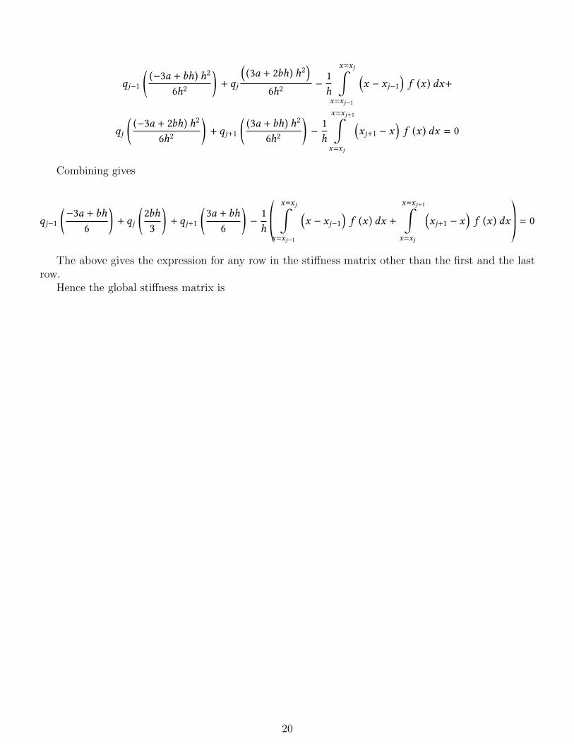
Combining gives

qj−1

(−3a + bh

6

)+ qj

(2bh3

)+ qj+1

(3a + bh

6

)−1h

*..,

x=x j∫x=x j−1

(x − xj−1

)f (x ) dx +

x=x j+1∫x=x j

(xj+1 − x

)f (x ) dx

+//-= 0

The above gives the expression for any row in the stiffness matrix other than the first and the lastrow.

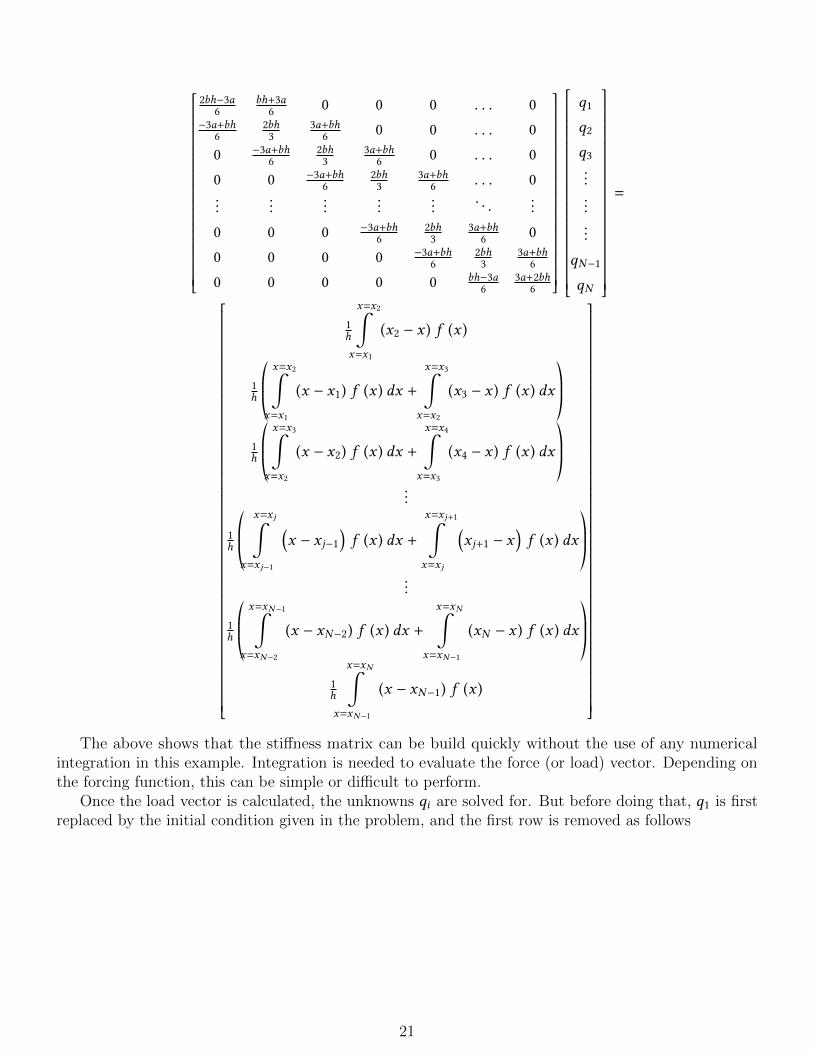
Hence the global stiffness matrix is

20

2bh−3a6

bh+3a6 0 0 0 . . . 0

−3a+bh6

2bh3

3a+bh6 0 0 . . . 0

0 −3a+bh6

2bh3

3a+bh6 0 . . . 0

0 0 −3a+bh6

2bh3

3a+bh6 . . . 0

......

......

.... . .

...

0 0 0 −3a+bh6

2bh3

3a+bh6 0

0 0 0 0 −3a+bh6

2bh3

3a+bh6

0 0 0 0 0 bh−3a6

3a+2bh6

q1

q2

q3.........

qN−1

qN

=

1h

x=x2∫x=x1

(x2 − x ) f (x )

1h

*..,

x=x2∫x=x1

(x − x1) f (x ) dx +

x=x3∫x=x2

(x3 − x ) f (x ) dx+//-

1h

*..,

x=x3∫x=x2

(x − x2) f (x ) dx +

x=x4∫x=x3

(x4 − x ) f (x ) dx+//-

...

1h

*..,

x=x j∫x=x j−1

(x − xj−1

)f (x ) dx +

x=x j+1∫x=x j

(xj+1 − x

)f (x ) dx

+//-

...

1h

*..,

x=xN−1∫x=xN−2

(x − xN−2) f (x ) dx +

x=xN∫x=xN−1

(xN − x ) f (x ) dx+//-

1h

x=xN∫x=xN−1

(x − xN−1) f (x )

The above shows that the stiffness matrix can be build quickly without the use of any numericalintegration in this example. Integration is needed to evaluate the force (or load) vector. Depending onthe forcing function, this can be simple or difficult to perform.

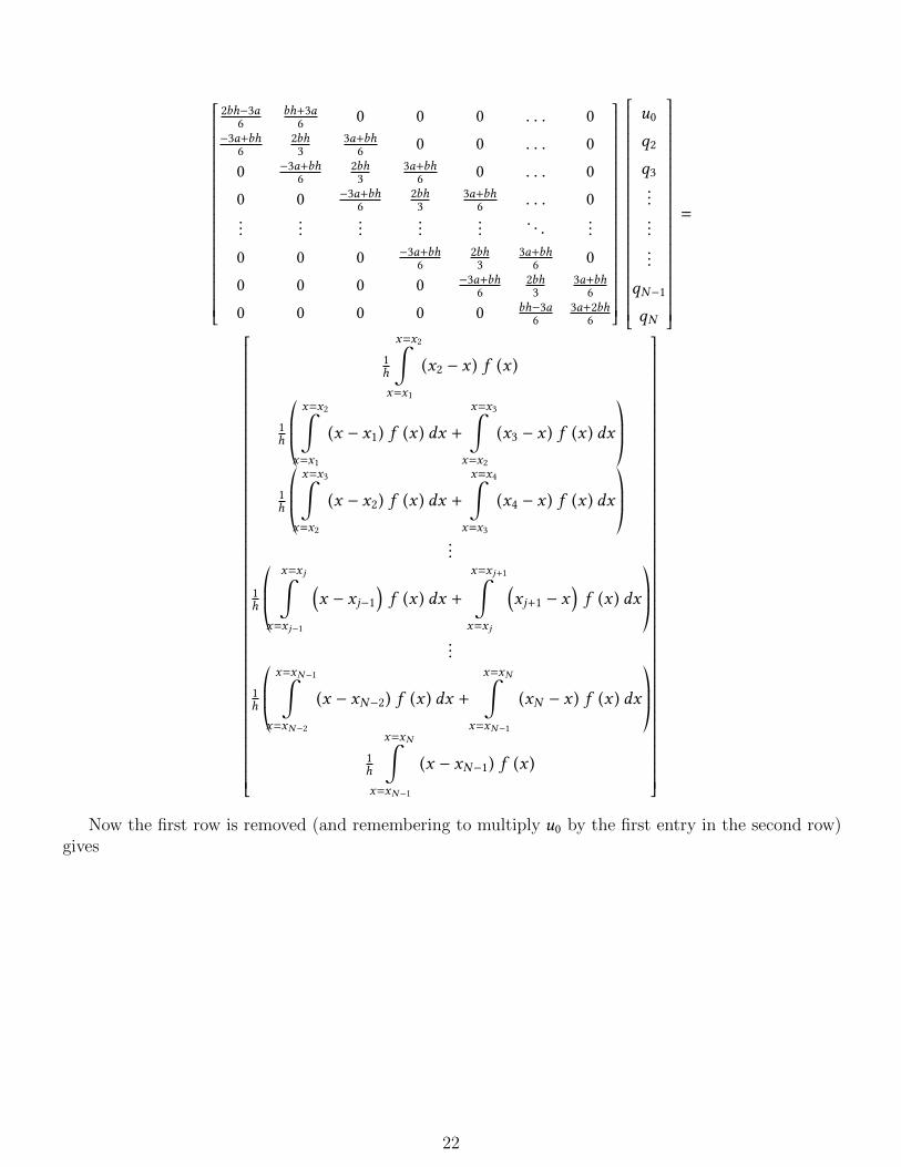
Once the load vector is calculated, the unknowns qi are solved for. But before doing that, q1 is firstreplaced by the initial condition given in the problem, and the first row is removed as follows

21

2bh−3a6

bh+3a6 0 0 0 . . . 0

−3a+bh6

2bh3

3a+bh6 0 0 . . . 0

0 −3a+bh6

2bh3

3a+bh6 0 . . . 0

0 0 −3a+bh6

2bh3

3a+bh6 . . . 0

......

......

.... . .

...

0 0 0 −3a+bh6

2bh3

3a+bh6 0

0 0 0 0 −3a+bh6

2bh3

3a+bh6

0 0 0 0 0 bh−3a6

3a+2bh6

u0

q2

q3.........

qN−1

qN

=

1h

x=x2∫x=x1

(x2 − x ) f (x )

1h

*..,

x=x2∫x=x1

(x − x1) f (x ) dx +

x=x3∫x=x2

(x3 − x ) f (x ) dx+//-

1h

*..,

x=x3∫x=x2

(x − x2) f (x ) dx +

x=x4∫x=x3

(x4 − x ) f (x ) dx+//-

...

1h

*..,

x=x j∫x=x j−1

(x − xj−1

)f (x ) dx +

x=x j+1∫x=x j

(xj+1 − x

)f (x ) dx

+//-

...

1h

*..,

x=xN−1∫x=xN−2

(x − xN−2) f (x ) dx +

x=xN∫x=xN−1

(xN − x ) f (x ) dx+//-

1h

x=xN∫x=xN−1

(x − xN−1) f (x )

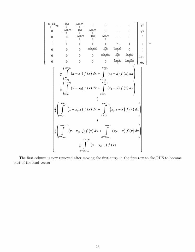
Now the first row is removed (and remembering to multiply u0 by the first entry in the second row)gives

22

−3a+bh6 u0

2bh3

3a+bh6 0 0 . . . 0

0 −3a+bh6

2bh3

3a+bh6 0 . . . 0

0 0 −3a+bh6

2bh3

3a+bh6 . . . 0

......

......

.... . .

...

0 0 0 −3a+bh6

2bh3

3a+bh6 0

0 0 0 0 −3a+bh6

2bh3

3a+bh6

0 0 0 0 0 bh−3a6

3a+2bh6

q2

q3.........

qN−1

qN

=

1h

*..,

x=x2∫x=x1

(x − x1) f (x ) dx +

x=x3∫x=x2

(x3 − x ) f (x ) dx+//-

1h

*..,

x=x3∫x=x2

(x − x2) f (x ) dx +

x=x4∫x=x3

(x4 − x ) f (x ) dx+//-

...

1h

*..,

x=x j∫x=x j−1

(x − xj−1

)f (x ) dx +

x=x j+1∫x=x j

(xj+1 − x

)f (x ) dx

+//-

...

1h

*..,

x=xN−1∫x=xN−2

(x − xN−2) f (x ) dx +

x=xN∫x=xN−1

(xN − x ) f (x ) dx+//-

1h

x=xN∫x=xN−1

(x − xN−1) f (x )

The first column is now removed after moving the first entry in the first row to the RHS to becomepart of the load vector

23

2bh3

3a+bh6 0 0 . . . 0

−3a+bh6

2bh3

3a+bh6 0 . . . 0

0 −3a+bh6

2bh3

3a+bh6 . . . 0

......

......

. . ....

0 0 −3a+bh6

2bh3

3a+bh6 0

0 0 0 −3a+bh6

2bh3

3a+bh6

0 0 0 0 bh−3a6

3a+2bh6

q2

q3.........

qN−1

qN

=

1h

*..,

x=x2∫x=x1

(x − x1) f (x ) dx +

x=x3∫x=x2

(x3 − x ) f (x ) dx+//-−

(−3a+bh

6 u0)

1h

*..,

x=x3∫x=x2

(x − x2) f (x ) dx +

x=x4∫x=x3

(x4 − x ) f (x ) dx+//-

...

1h

*..,

x=x j∫x=x j−1

(x − xj−1

)f (x ) dx +

x=x j+1∫x=x j

(xj+1 − x

)f (x ) dx

+//-

...

1h

*..,

x=xN−1∫x=xN−2

(x − xN−2) f (x ) dx +

x=xN∫x=xN−1

(xN − x ) f (x ) dx+//-

1h

x=xN∫x=xN−1

(x − xN−1) f (x )

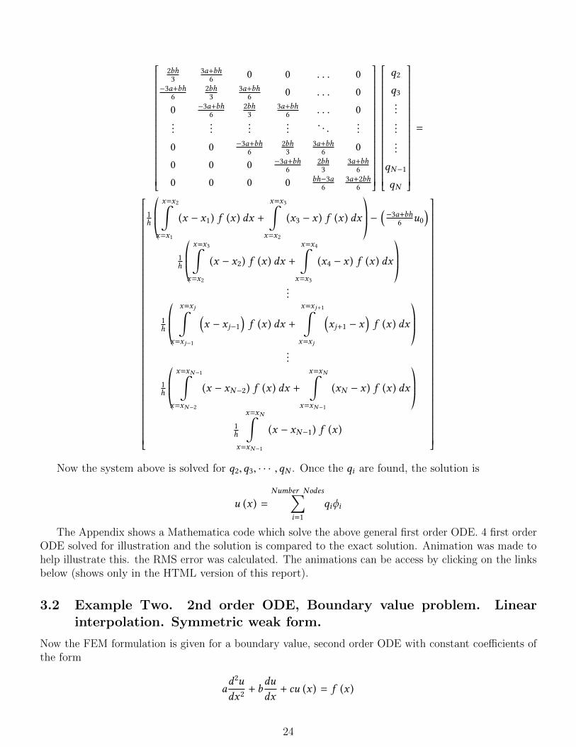
Now the system above is solved for q2,q3, · · · ,qN . Once the qi are found, the solution is

u (x ) =Number Nodes∑

i=1

qiϕi

The Appendix shows a Mathematica code which solve the above general first order ODE. 4 first orderODE solved for illustration and the solution is compared to the exact solution. Animation was made tohelp illustrate this. the RMS error was calculated. The animations can be access by clicking on the linksbelow (shows only in the HTML version of this report).

3.2 Example Two. 2nd order ODE, Boundary value problem. Linearinterpolation. Symmetric weak form.

Now the FEM formulation is given for a boundary value, second order ODE with constant coefficients ofthe form

ad2u

dx2+ b

du

dx+ cu (x ) = f (x )

24

with the initial conditions u (x0) = u0 (called essential Dirichlet condition), and the Neumann boundarycondition du

dx = β at L, for x0 ≤ x ≤ LAs before, the solution is assumed to be of the form

u =N∑i=1

qiϕi

And the unknown q are found by solving N algebraic equations

L∫x0

ϕjR (x ) dx = 0 j = 1 · · ·N

Where R (x ) is the ODE residual obtained by substituting the assumed solution into the originalODE. Hence the above becomes (For simplicity, j = 1 · · ·N is not written each time as it is assumed tobe the case)

L∫x0

ϕj

(ad2u

dx2+ b

du

dx+ cu (x ) − f (x )

)dx = 0

L∫x0

ϕjad2u

dx2dx +

L∫x0

ϕj

(bdu

dx+ cu (x ) − f (x )

)dx = 0taдA1 (1)

Applying integration by parts on

L∫x0

ϕjad2udx2

dx . Since

d

dx

(a ϕj

du

dx

)= aϕj

d2u

dx2+ aϕ′j

du

dx

then integrating both sides of the above gives

L∫x0

d

dx

(a ϕj

du

dx

)dx =

L∫x0

aϕjd2u

dx2dx +

L∫x0

aϕ′jdu

dxdx

[aϕj

du

dx

] L

x0

=

L∫x0

aϕjd2u

dx2dx +

L∫x0

aϕ′jdu

dxdx

HenceL∫

x0

aϕjd2u

dx2dx =

[aϕj

du

dx

] L

x0

−

L∫x0

aϕ′jdu

dxdx

Substituting the above in equation A1 gives

[aϕj

du

dx

] L

x0

−

L∫x0

aϕ′jdu

dxdx +

L∫x0

ϕj

(bdu

dx+ cu (x ) − f (x )

)dx = 0 (A2)

25

Consider the term [aϕj

du

dx

] L

x0

= aϕjdu

dx

x=L− aϕj

du

dx

x=x0First consider the term aϕj

dudx

x=L. Sincedudx = β at L then this term becomes aβ

[ϕj

]x=L

. But[ϕj

]x=L

is non zero only for the N th shape function evaluated at x = L. Since linear interpolation is used, the N th

shape function is ϕN =x−xN−1

h which have the value of 1 at x = xN . Hence

aϕjdu

dx

x=L= aβ whenj = Notherwise0

Now consider the term aϕjdudx

x=x0 , since at x = x0 all shape functions will be zero except for ϕ1 which

has the value of 1 at x = x0. Hence this simplifies to adudx

x=x0

recalling that dudx =

ddx

N∑i=1

qiϕi =N∑i=1

qiϕ′i .

But at x = x0 only ϕ1 is defined and its has the slope of −1h , hence

adu

dx

x=x0=−aq1h

when j = 1, otherwise 0

However, q1 = u0 since that is by definition the initial condition. Finally one obtains

[aϕj

du

dx

] L

x0

=

aq1h j = 1

aβ j = N

Hence the symmetric weak form equation A2 can now be simplified more giving

aq1h j = 1

aβ j = N

−

L∫x0

aϕ′jdu

dxdx +

L∫x0

ϕj

(bdu

dx+ cu (x ) − f (x )

)dx = 0 j = 1 · · ·N (A3)

The trial function obtain by linear interpolation are used. These are shown again in this table

i ϕi ϕ′i

1 (x2−x )h

−1h

1 < i < N(x−xi−1)

h , (xi+1−x )h

1h ,−1h

N (x−xN−1)h

1h

The global stiffness matrix is now constructed. For the first equation (which corresponds to the firstrow in the global stiffness matrix) the result is

aq1h−

L∫x0

aϕ′1du

dxdx +

L∫x0

ϕ1

(bdu

dx+ cu (x ) − f (x )

)dx = 0

Since u =N∑i=1

qiϕi , and since ϕ1 domain of influence is only from x1 to x2 then above becomes

26

aq1h−

x2∫x1

aϕ′1d

dx(q1ϕ1 + q2ϕ2) dx +

x2∫x1

ϕ1

(bd

dx(q1ϕ1 + q2ϕ2) + c (q1ϕ1 + q2ϕ2) − f (x )

)dx = 0

But ϕ1 =(x2−x )

h and ϕ′1 =−1h and over the domain from x1 to x2, ϕ2 =

(x−x1)h ,ϕ′2 =

1h , hence the above

becomes

aq1h−

x2∫x1

−a

h

(−q1h+q2h

)dx +

x2∫x1

(x2 − x )

h

(b

(−q1h+q2h

)+ c

(q1

(x2 − x )

h+ q2

(x − x1)

h

)− f (x )

)dx = 0

The above simplifies to

aq1h−q1h2

(ax1 −

b (x1 − x2)2

2−c (x1 − x2)3

3− ax2

)+q2h2

(−ax1 +

b (x1 − x2)2

2−c (x1 − x2)3

6+ ax2

)−

1h

x2∫x1

(x2 − x ) f (x ) = 0

−q1h2

(−ah + ax1 −

b (x1 − x2)2

2−c (x1 − x2)3

3− ax2

)+q2h2

(−ax1 +

b (x1 − x2)2

2−c (x1 − x2)3

6+ ax2

)−

1h

x2∫x1

(x2 − x ) f (x ) = 0

The above gives the first row in the stiffness matrix. Since it is assumed that each element will havethe same length, hence x1 − x2 = −h, and the above becomes

−q1h2

(−ah + ax1 −

bh2

2+ch3

3− ax2

)+q2h2

(−ax1 +

bh2

2+ch3

6+ ax2

)−1h

x2∫x1

(x2 − x ) f (x ) = 0

−q1

(−a

h+ax1h2−b

2+ch

3−ax2h2

)+ q2

(−ax1h2+b

2+ch

6+ax2h2

)−1h

x2∫x1

(x2 − x ) f (x ) = 0

For the last equation, which will be the last row in the global stiffness matrix

aβ −

xN∫xN−1

aϕ′Ndu

dxdx +

xN∫xN−1

ϕN

(bdu

dx+ cu (x ) − f (x )

)dx = 0

Since u =N∑i=1

qiϕi , and since ϕN domain of influence is only from xN−1 to xN The above becomes

aβ−

xN∫xN−1

aϕ′Nd

dx(qN−1ϕN−1 + qNϕN ) dx+

xN∫xN−1

ϕN

(bd

dx(qN−1ϕN−1 + qNϕN ) + c (qN−1ϕN−1 + qNϕN ) − f (x )

)dx = 0

But ϕN =(x−xN−1)

h and ϕ′N =1h and over the domain from xN−1 to xN , ϕN−1 =

(xN−x )h ,ϕ′N−1 =

−1h hence

the above becomes

27

aβ −

xN∫xN−1

a

h

(qN−1

(−1h

)+ qN

1h

)dx+

xN∫xN−1

(x − xN−1)

h

(b

(qN−1

(−1h

)+ qN

1h

)+ c

(qN−1

(xN − x )

h+ qN

(x − xN−1)

h

)− f (x )

)dx = 0

The above simplifies to

aβ −qN−1h2

(−axN−1 −

b (xN−1 − xN )2

2−c (xN−1 − xN )

3

6+ axN

)+

qNh2

(+axN−1 +

b (xN−1 − xN )2

2−c (xN−1 − xN )

3

3− axN

)−1h

xN∫xN−1

(x − xN−1) f (x ) = 0

The above represents the last row in the global stiffness matrix. Since it is assumed that each elementwill have the same length, hence xN−1 − xN = −h, and the above becomes

aβ −qN−1h2

(−axN−1 −

bh2

2+ch3

6+ axN

)+qNh2

(axN−1 +

bh2

2+ch3

3− axN

)−1h

xN∫xN−1

(x − xN−1) f (x ) = 0

aβ − qN−1

(−axN−1h2

−b

2+ch

6+axNh2

)+ qN

(axN−1h2

+b

2+ch

3−axNh2

)−1h

xN∫xN−1

(x − xN−1) f (x ) = 0

The expression for any row in between the first and the last rows is now found. For a general node jthe result is

−

x j+1∫x j−1

aϕ′jdu

dxdx +

x j+1∫x j−1

ϕj

(bdu

dx+ cu (x ) − f (x )

)dx = 0

Breaking the integral into halves to make it easier to write the trial functions over the domain ofinfluence gives

−*..,

x j∫x j−1

aϕ′jdu

dxdx +

x j+1∫x j

aϕ′jdu

dxdx

+//-+

x j∫x j−1

ϕj

(bdu

dx+ cu (x ) − f (x )

)dx +

x j+1∫x j

ϕj

(bdu

dx+ cu (x ) − f (x )

)dx = 0

Considering the first domain xj−1 ≤ x ≤ xj gives

−

x j∫x j−1

aϕ′jdu

dxdx +

x j∫x j−1

ϕj

(bdu

dx+ cu (x ) − f (x )

)dx

Over this range, u = qj−1ϕj−1 + qjϕj hencedudx = qj−1ϕ

′j−1 + qjϕ

′j where ϕj−1 =

x j−xh ,ϕ

′j−1 =

−1h ,ϕj =

x−x j−1h ,ϕ′j =

1h hence the above becomes

28

−

x j∫x j−1

a1h

(qj−1

(−1h

)+ qj

1h

)dx +

x j∫x j−1

x − xj−1

h

(b

(qj−1

(−1h

)+ qj

1h

)+ c

(qj−1

xj − x

h+ qj

x − xj−1

h

)− f (x )

)dx

(A4)Now considering the second domain xj ≤ x ≤ xj+1 gives

−

x j+1∫x j

aϕ′jdu

dxdx +

x j+1∫x j

ϕj

(bdu

dx+ cu (x ) − f (x )

)dx

Over this range, u = qjϕj + qj+1ϕj+1 hence dudx = qjϕ

′j + qj+1ϕ

′j+1 where ϕj =

x j+1−xh ,ϕ′j =

−1h ,ϕj+1 =

x−x jh ,ϕ

′j+1 =

1h hence the above becomes

−

x j+1∫x j

(−a

h

) (−qj

h+qj+1

h

)dx+

x j+1∫x j

xj+1 − x

h

(b

(−qj

h+ qj+1

1h

)+ c

(qjxj+1 − x

h+ qj+1

x − xj

h

)− f (x )

)dx (A5)

Combine A4 and A5 and simplify we obtain

qj−1

h2*.,−axj−1 −

b(xj−1 − xj

) 22

−c(xj−1 − xj

) 36

+ axj+/-

+qj

h2*.,axj−1 +

b(xj−1 − xj

) 22

−c(xj−1 − xj

) 33

−b

(xj − xj+1

) 22

−c(xj − xj+1

) 33

− axj+1+/-

+qj+1

h2*.,−axj +

b(xj − xj+1

) 22

−c(xj − xj+1

) 36

+ axj+1+/-−

x j∫x j−1

x − xj−1

hf (x ) dx −

x j+1∫x j

xj+1 − x

hdx = 0

Since we are assuming each element will have the same length, hence xj−1 − xj = −h, xj − xj+1 = −hand the above becomes

qj−1

(−axj−1

h2−b

2+ch

6+axj

h2

)+qj

(axj−1

h2+2ch3−axj+1

h2

)

+qj+1

(−axj

h2+b

2+ch

6+axj+1

h2

)−

x j∫x j−1

x − xj−1

hf (x ) dx −

x j+1∫x j

xj+1 − x

hf (x ) dx = 0

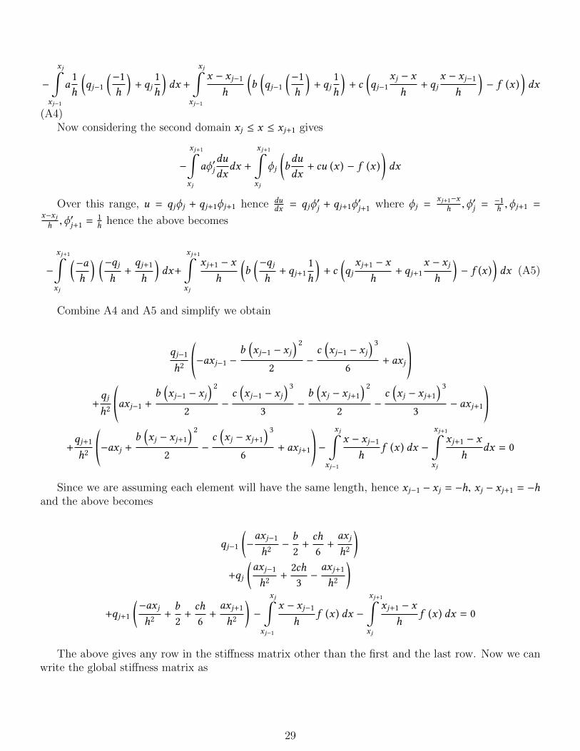
The above gives any row in the stiffness matrix other than the first and the last row. Now we canwrite the global stiffness matrix as

29

(−ah +

ax1h2− b

2 +ch3 −

ax2h2

) (−ax1h2+ b

2 −ch6 +

ax2h2

)0 0(

−ax1h2− b

2 +ch6 +

ax2h2

) (ax1h2+ 2ch

3 −ax3h2

) (−ax2h2+ b

2 +ch6 +

ax3h2

)0

0(−ax j−1h2− b

2 +ch6 +

ax jh2

) (ax j−1h2+ 2ch

3 −ax j+1h2

) (−ax jh2+ b

2 +ch6 +

ax j+1h2

)0 0

. . . · · ·

0 0(−axN−1h2− b

2 +ch6 +

axNh2

) (axN−1h2+ b

2 +ch3 −

axNh2

)

q1

q2......

qj...

qN−1

qN

=

1h

x2∫x1

(x2 − x ) f (x )

...

...

...

1h

x j∫x j−1

(x − xj−1

)f (x ) dx + 1

h

x j+1∫x j

(xj+1 − x

)f (x ) dx

...

...

1h

xN∫xN−1

(x − xN−1) f (x ) − aβ

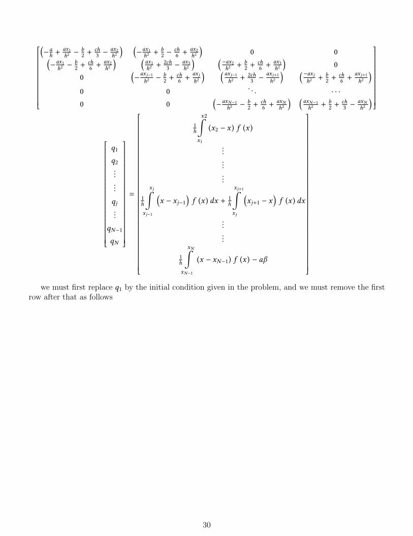
we must first replace q1 by the initial condition given in the problem, and we must remove the firstrow after that as follows

30

(−ah +

ax1h2− b

2 +ch3 −

ax2h2

) (−ax1h2+ b

2 −ch6 +

ax2h2

)0 0(

−ax1h2− b

2 +ch6 +

ax2h2

) (ax1h2+ 2ch

3 −ax3h2

) (−ax2h2+ b

2 +ch6 +

ax3h2

)0

0 0. . . · · ·

0 0. . . · · ·

0 0(−axN−1h2− b

2 +ch6 +

axNh2

) (axN−1h2+ b

2 +ch3 −

axNh2

)

u0

q2......

qj...

qN−1

qN

=

1h

x2∫x1

(x2 − x ) f (x )

...

...

...

1h

x j∫x j−1

(x − xj−1

)f (x ) dx + 1

h

x j+1∫x j

(xj+1 − x

)f (x ) dx

...

...

1h

xN∫xN−1

(x − xN−1) f (x ) − aβ

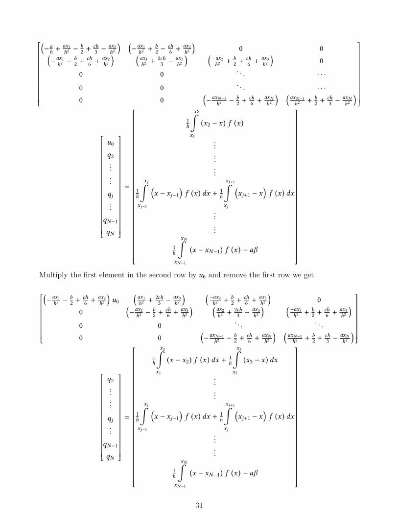
Multiply the first element in the second row by u0 and remove the first row we get

(−ax1h2− b

2 +ch6 +

ax2h2

)u0

(ax1h2+ 2ch

3 −ax3h2

) (−ax2h2+ b

2 +ch6 +

ax3h2

)0

0(−ax2h2− b

2 +ch6 +

ax3h2

) (ax2h2+ 2ch

3 −ax4h2

) (−ax3h2+ b

2 +ch6 +

ax4h2

)0 0

. . .. . .

0 0(−axN−1h2− b

2 +ch6 +

axNh2

) (axN−1h2+ b

2 +ch3 −

axNh2

)

q2......

qj...

qN−1

qN

=

1h

x2∫x1

(x − x2) f (x ) dx + 1h

x3∫x2

(x3 − x ) dx

...

...

1h

x j∫x j−1

(x − xj−1

)f (x ) dx + 1

h

x j+1∫x j

(xj+1 − x

)f (x ) dx

...

...

1h

xN∫xN−1

(x − xN−1) f (x ) − aβ

31

Now move the first element of the first row above to the RHS and remove the first column we obtain

(ax1h2+ 2ch

3 −ax3h2

) (−ax2h2+ b

2 +ch6 +

ax3h2

)0 0

0(−ax2h2− b

2 +ch6 +

ax3h2

) (ax2h2+ 2ch

3 −ax4h2

) (−ax jh2+ b

2 +ch6 +

ax j+1h2

)...

. . . · · ·. . .

0 0(−axN−1h2− b

2 +ch6 +

axNh2

) (axN−1h2+ b

2 +ch3 −

axNh2

)

q2......

qj...

qN−1

qN

=

1h

x2∫x1

(x − x2) f (x ) dx + 1h

x3∫x2

(x3 − x ) dx −(−ax1h2− b

2 +ch6 +

ax2h2

)u0

...

...

1h

x j∫x j−1

(x − xj−1

)f (x ) dx + 1

h

x j+1∫x j

(xj+1 − x

)f (x ) dx

...

...

1h

xN∫xN−1

(x − xN−1) f (x ) − aβ

Now we solve for the vector [q2,q3, · · · ,qN ]T and this completes our solution.

A Matlab implementation is below which solves any second order ODE. This code was used togenerate an animation. This animation can be accessed by clicking on the link below.

4 References

1. Methods of computer modeling in engineering and the sciences. Volume 1. By Professor Satya N.Atluri. Tech Science Press.

2. Class lecture notes. MAE 207. Computational methods. UCI. Spring 2006. Instructor: ProfessorSN Atluri.

3. Computational techniques for fluid dynamics, Volume I. C.A.J.Fletcher. Springer-Verlag

32