Embed Size (px)
Citation preview

T. Schulthess17th Workshop on HPC in Meteorology @ ECMWF, Reading, Wednesday October 26, 2016
Thomas C. Schulthess
1
Exascale computing: endgame or new beginning for climate modelling
T. Schulthess17th Workshop on HPC in Meteorology @ ECMWF, Reading, Wednesday October 26, 2016
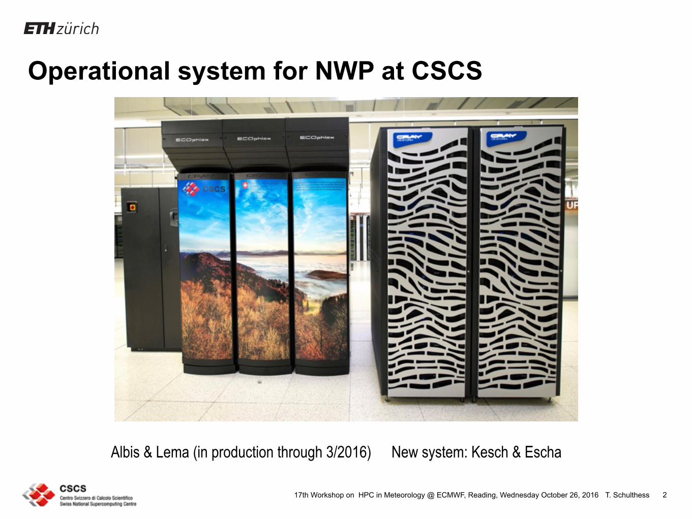
Operational system for NWP at CSCS
2
Albis & Lema (in production through 3/2016) New system: Kesch & Escha
T. Schulthess17th Workshop on HPC in Meteorology @ ECMWF, Reading, Wednesday October 26, 2016
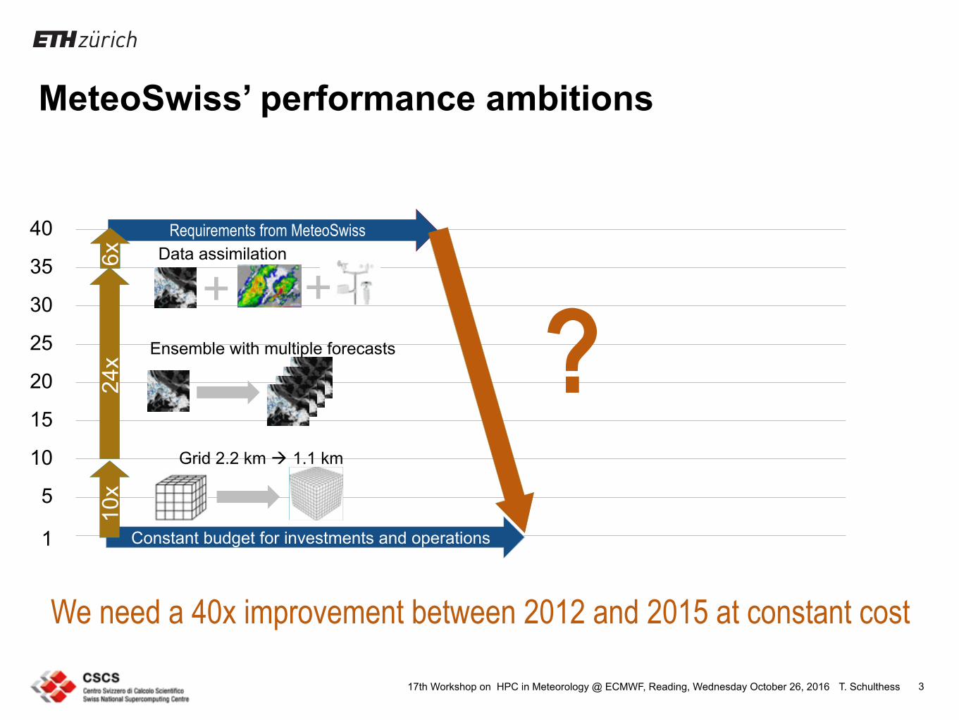
MeteoSwiss’ performance ambitions
3
1
5
10
15
20
25
30
35
40
Constant budget for investments and operations
24x Ensemble with multiple forecasts
Grid 2.2 km ! 1.1 km
10x
Requirements from MeteoSwissData assimilation6x
We need a 40x improvement between 2012 and 2015 at constant cost
?
T. Schulthess17th Workshop on HPC in Meteorology @ ECMWF, Reading, Wednesday October 26, 2016 4
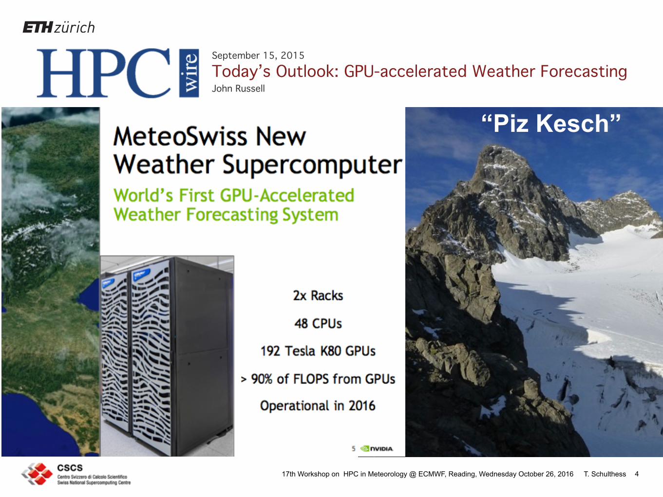
September 15, 2015
Today’s Outlook: GPU-accelerated Weather ForecastingJohn Russell
“Piz Kesch”
T. Schulthess17th Workshop on HPC in Meteorology @ ECMWF, Reading, Wednesday October 26, 2016 5
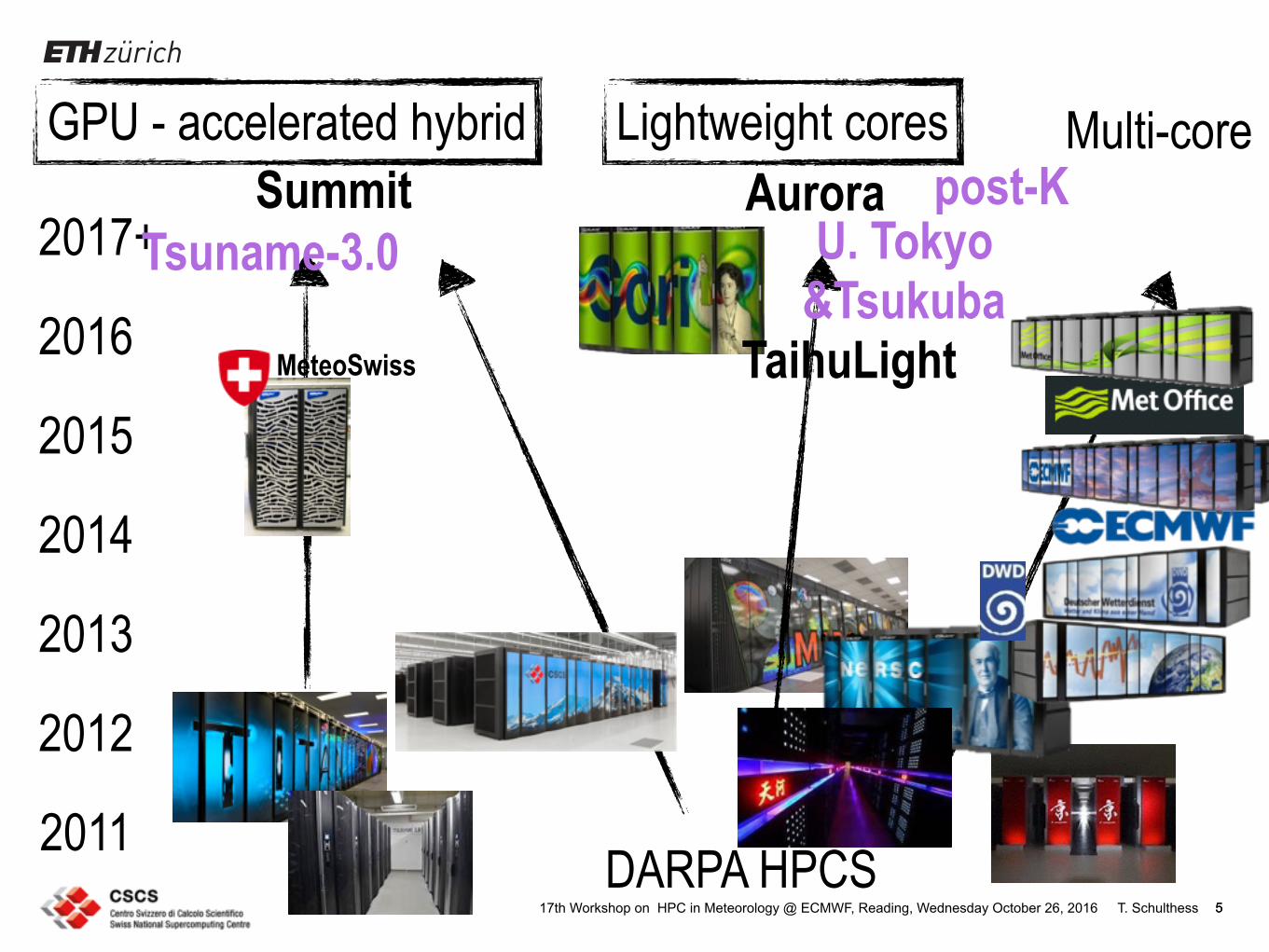
2012
2013
2014
2015
2016
2017+Summit Aurora
Lightweight coresGPU - accelerated hybrid
DARPA HPCS
Tsuname-3.0 U. Tokyo &Tsukuba
2011
post-KMulti-core
MeteoSwiss
5
TaihuLight

T. Schulthess17th Workshop on HPC in Meteorology @ ECMWF, Reading, Wednesday October 26, 2016 6
State of the art implementation of new system for MeteoSwiss
• New system needs to be installed Q3/2015
• Assuming 2x improvement in per-socket performance:~20x more X86 sockets would require 30 Cray XC cabinets
Current Cray XC30/XC40 platform (space for 40 racks XC)
New system for Meteo Swiss if we build it like the German Weather Service (DWD) did theirs, or UK Met Office, or ECMWF … (30 racks XC)
Albis & Lema: 3 cabinets Cray XE6 installed Q2/2012
Thinking inside the box was not a good option!CSCS machine room
6
T. Schulthess17th Workshop on HPC in Meteorology @ ECMWF, Reading, Wednesday October 26, 2016
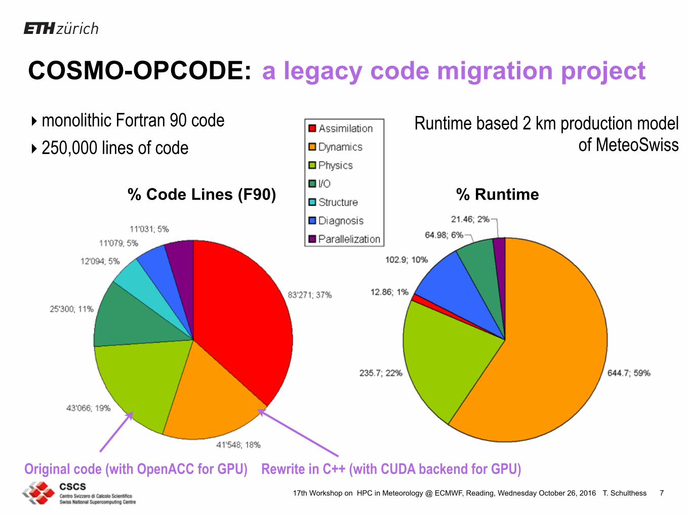
COSMO-OPCODE:
7
% Code Lines (F90) % Runtime
Runtime based 2 km production model of MeteoSwiss
Original code (with OpenACC for GPU) Rewrite in C++ (with CUDA backend for GPU)
‣monolithic Fortran 90 code ‣ 250,000 lines of code
a legacy code migration project
T. Schulthess17th Workshop on HPC in Meteorology @ ECMWF, Reading, Wednesday October 26, 2016
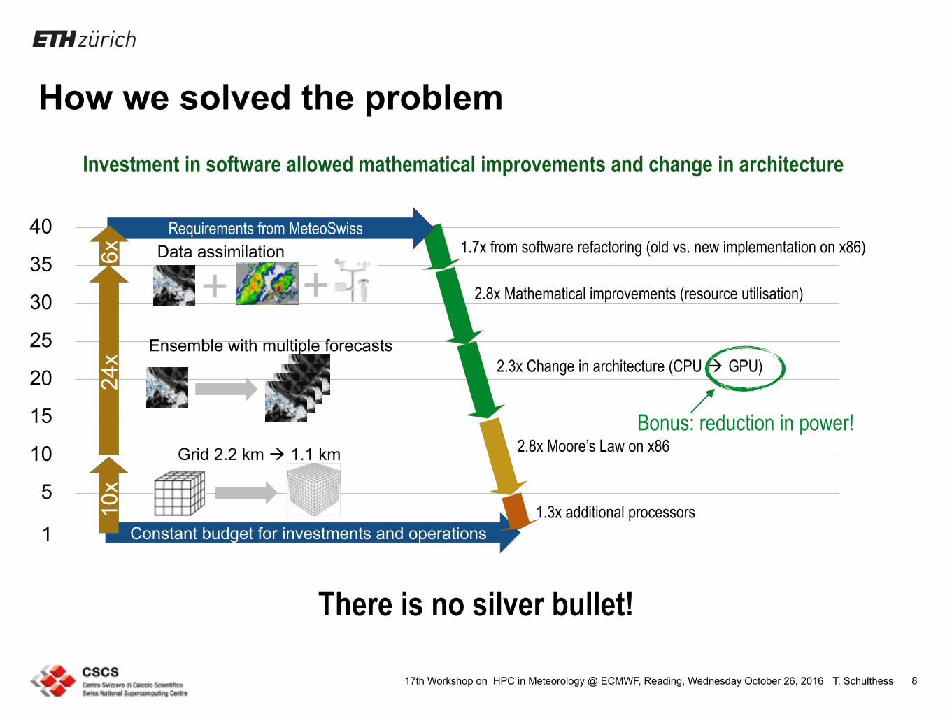
How we solved the problem
8
1
5
10
15
20
25
30
35
40
Constant budget for investments and operations
Grid 2.2 km ! 1.1 km
24x Ensemble with multiple forecasts
Data assimilation
10x
1.7x from software refactoring (old vs. new implementation on x86)
2.8x Mathematical improvements (resource utilisation)
2.8x Moore’s Law on x86
2.3x Change in architecture (CPU ! GPU)
1.3x additional processors
Requirements from MeteoSwiss
6x
Investment in software allowed mathematical improvements and change in architecture
There is no silver bullet!
Bonus: reduction in power!

T. Schulthess25 Years CSCS, Lugano, Wednesday October 19, 2016 9
$500,000,000 $2,000,000,000
$13,000Source: Andy Keane @ ISC’10
Why commodity processors?
T. Schulthess17th Workshop on HPC in Meteorology @ ECMWF, Reading, Wednesday October 26, 2016 10
T. Schulthess17th Workshop on HPC in Meteorology @ ECMWF, Reading, Wednesday October 26, 2016
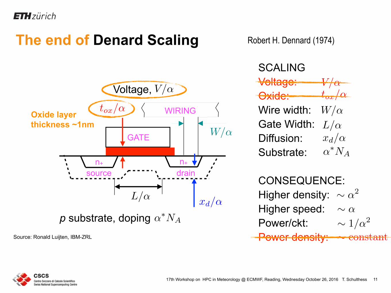
The end of Denard Scaling
11
L/
W/
tox
/
xd/
NA 1/2
constant
n+ n+
source drain
GATE
WIRING
p substrate, doping
Voltage, V/
SCALING Voltage: Oxide: Wire width: Gate Width: Diffusion: Substrate:
CONSEQUENCE: Higher density: Higher speed: Power/ckt: Power density:
V/tox
/
W/
L/
NA
xd/
↵2
↵
Oxide layer thickness ~1nm
Source: Ronald Luijten, IBM-ZRL
The end of Robert H. Dennard (1974)
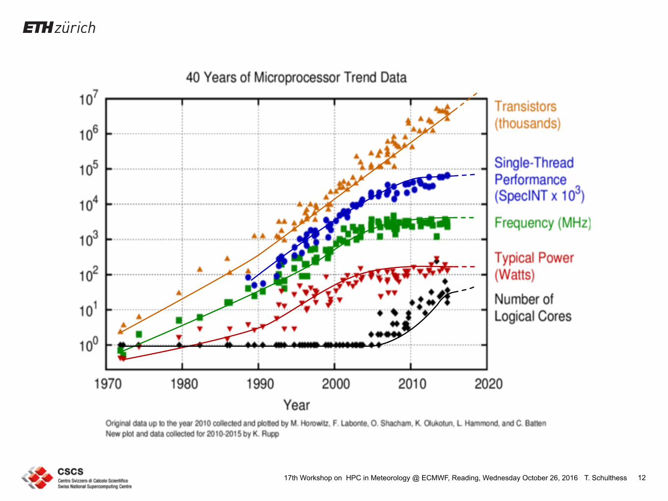
T. Schulthess17th Workshop on HPC in Meteorology @ ECMWF, Reading, Wednesday October 26, 2016 12
T. Schulthess17th Workshop on HPC in Meteorology @ ECMWF, Reading, Wednesday October 26, 2016
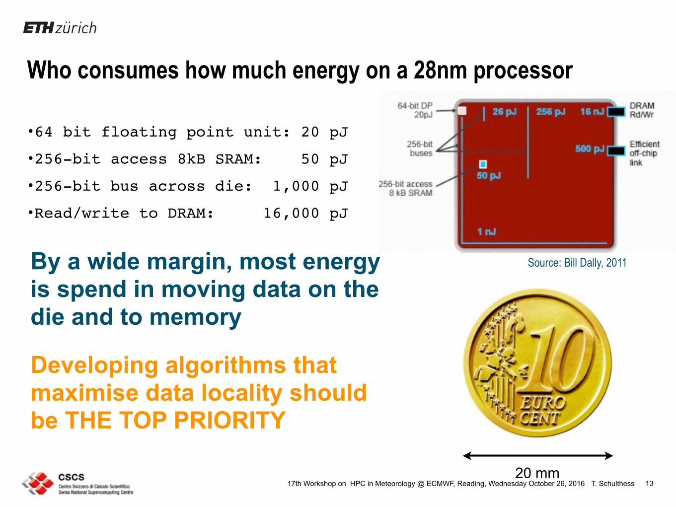
Who consumes how much energy on a 28nm processor
13
•64 bit floating point unit: 20 pJ
•256-bit access 8kB SRAM: 50 pJ
•256-bit bus across die: 1,000 pJ
•Read/write to DRAM: 16,000 pJ
20 mm
Source: Bill Dally, 2011By a wide margin, most energy is spend in moving data on the die and to memory
Developing algorithms that maximise data locality should be THE TOP PRIORITY
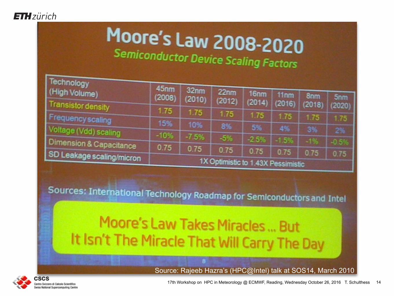
T. Schulthess17th Workshop on HPC in Meteorology @ ECMWF, Reading, Wednesday October 26, 2016 14
Source: Rajeeb Hazra’s (HPC@Intel) talk at SOS14, March 2010

T. Schulthess17th Workshop on HPC in Meteorology @ ECMWF, Reading, Wednesday October 26, 2016
“Piz Daint”
15
Cray XC30 with 5272 hybrid, GPU accelerated compute nodes
Compute node: > Host: Intel Xeon E5 2670 (SandyBridge 8c) > Accelerator: One NVIDIA K20X GPU (GK110)
13 m (~0.43 µs)
2.5 GHz (~0.38 ns)
0.73 GHz (~1.4ns)
Latency (μs) Bandwidth (GB/s)Aries chip 1.28 9.89Within Chassis 1.61 9.65Between Chassis 1.58 9.82Between Groups 2.53 9.63

T. Schulthess17th Workshop on HPC in Meteorology @ ECMWF, Reading, Wednesday October 26, 2016
Architectural diversity is here to stay, because it is a consequence of the dusk of CMOS scaling
(Moore’s Law)
16
What are the implications?
Complexity in software is one, but we don’t understand all implications
Physics of the computer matters more than ever
T. Schulthess17th Workshop on HPC in Meteorology @ ECMWF, Reading, Wednesday October 26, 2016 17
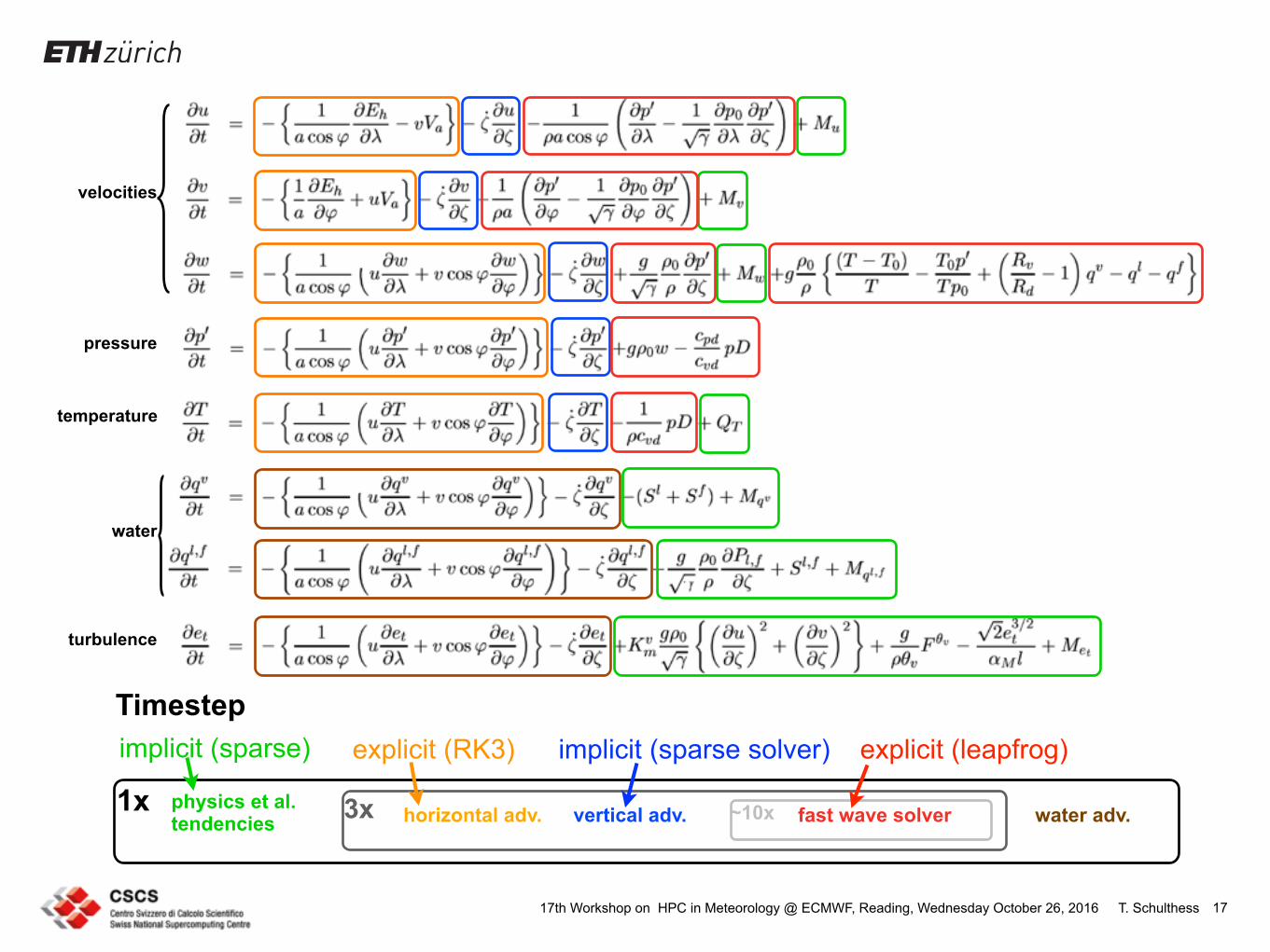
velocities
pressure
temperature
water
turbulence
physics et al. tendencies vertical adv. water adv.horizontal adv.3x fast wave solver~10x1x
Timestepexplicit (leapfrog)implicit (sparse solver)explicit (RK3)implicit (sparse)

T. Schulthess17th Workshop on HPC in Meteorology @ ECMWF, Reading, Wednesday October 26, 2016
Stencil example: Laplace operator in 2D
18
lap(i,j,k) = –4.0 * data(i,j,k) + data(i+1,j,k) + data(i-1,j,k) + data(i,j+1,k) + data(i,j-1,k);

T. Schulthess17th Workshop on HPC in Meteorology @ ECMWF, Reading, Wednesday October 26, 2016 19
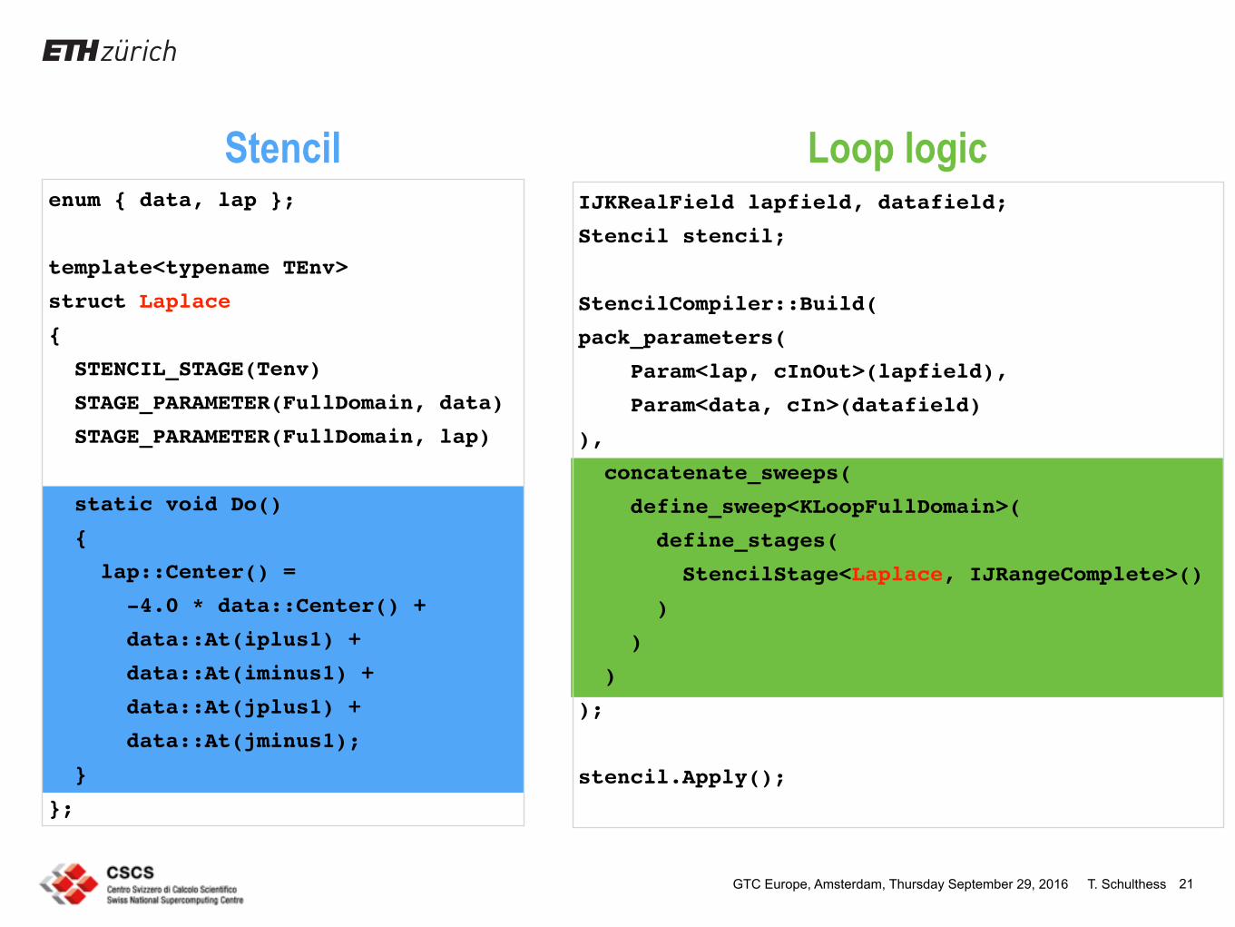
1. Loop-logic defines stencil application domain and order2. Stencil defines the operator to be applied
do k = kstart, kend do j = jstart, jend do i = istart, iend lap(i, j, k) = -4.0 * data(i, j , k) + & data(i+1, j, , k) + data(i-1, j , k) + & data(i , j+1, k) + data(i , j-1, k) end do end doend do
Two main components of an operator on a structured grid
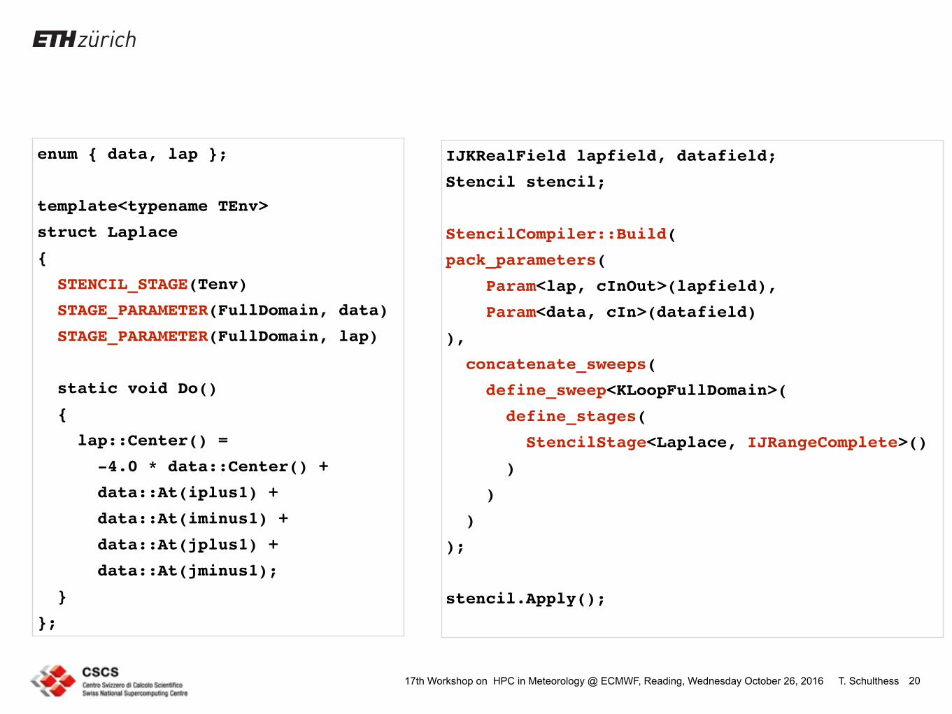
T. Schulthess17th Workshop on HPC in Meteorology @ ECMWF, Reading, Wednesday October 26, 2016 20
IJKRealField lapfield, datafield;
Stencil stencil;
StencilCompiler::Build(
pack_parameters(
Param<lap, cInOut>(lapfield),
Param<data, cIn>(datafield)
),
concatenate_sweeps(
define_sweep<KLoopFullDomain>(
define_stages(
StencilStage<Laplace, IJRangeComplete>()
)
)
)
);
stencil.Apply();
enum data, lap ;
template<typename TEnv>
struct Laplace
STENCIL_STAGE(Tenv)
STAGE_PARAMETER(FullDomain, data)
STAGE_PARAMETER(FullDomain, lap)
static void Do()
lap::Center() =
-4.0 * data::Center() +
data::At(iplus1) +
data::At(iminus1) +
data::At(jplus1) +
data::At(jminus1);
;
T. SchulthessGTC Europe, Amsterdam, Thursday September 29, 2016 21
enum data, lap ;
template<typename TEnv>
struct Laplace
STENCIL_STAGE(Tenv)
STAGE_PARAMETER(FullDomain, data)
STAGE_PARAMETER(FullDomain, lap)
static void Do()
lap::Center() =
-4.0 * data::Center() +
data::At(iplus1) +
data::At(iminus1) +
data::At(jplus1) +
data::At(jminus1);
;
IJKRealField lapfield, datafield;
Stencil stencil;
StencilCompiler::Build(
pack_parameters(
Param<lap, cInOut>(lapfield),
Param<data, cIn>(datafield)
),
concatenate_sweeps(
define_sweep<KLoopFullDomain>(
define_stages(
StencilStage<Laplace, IJRangeComplete>()
)
)
)
);
stencil.Apply();
Stencil Loop logic
T. SchulthessGTC Europe, Amsterdam, Thursday September 29, 2016 22
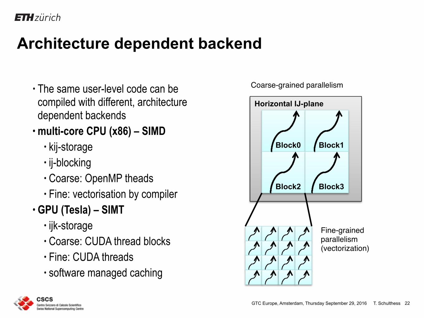
Architecture dependent backend
• The same user-level code can be compiled with different, architecture dependent backends
• multi-core CPU (x86) – SIMD • kij-storage • ij-blocking • Coarse: OpenMP theads • Fine: vectorisation by compiler
• GPU (Tesla) – SIMT • ijk-storage • Coarse: CUDA thread blocks • Fine: CUDA threads • software managed caching
STELLA backends
• The same high-level user code can be compiled using different backends
• CPU (x86 multi-core) • kij-storage • ij-blocking • Coarse: OpenMP threads • Fine: vectorization by compiler
• GPU (NVIDIA) • ijk-storage • Coarse: CUDA thread blocks • Fine: CUDA threads • software managed caching
A single switch chooses the
STELLA backend
Horizontal IJ-plane
Block0 Block1
Block2 Block3
Coarse-grained parallelism"
Fine-grained parallelism (vectorization)"
T. SchulthessGTC Europe, Amsterdam, Thursday September 29, 2016 23
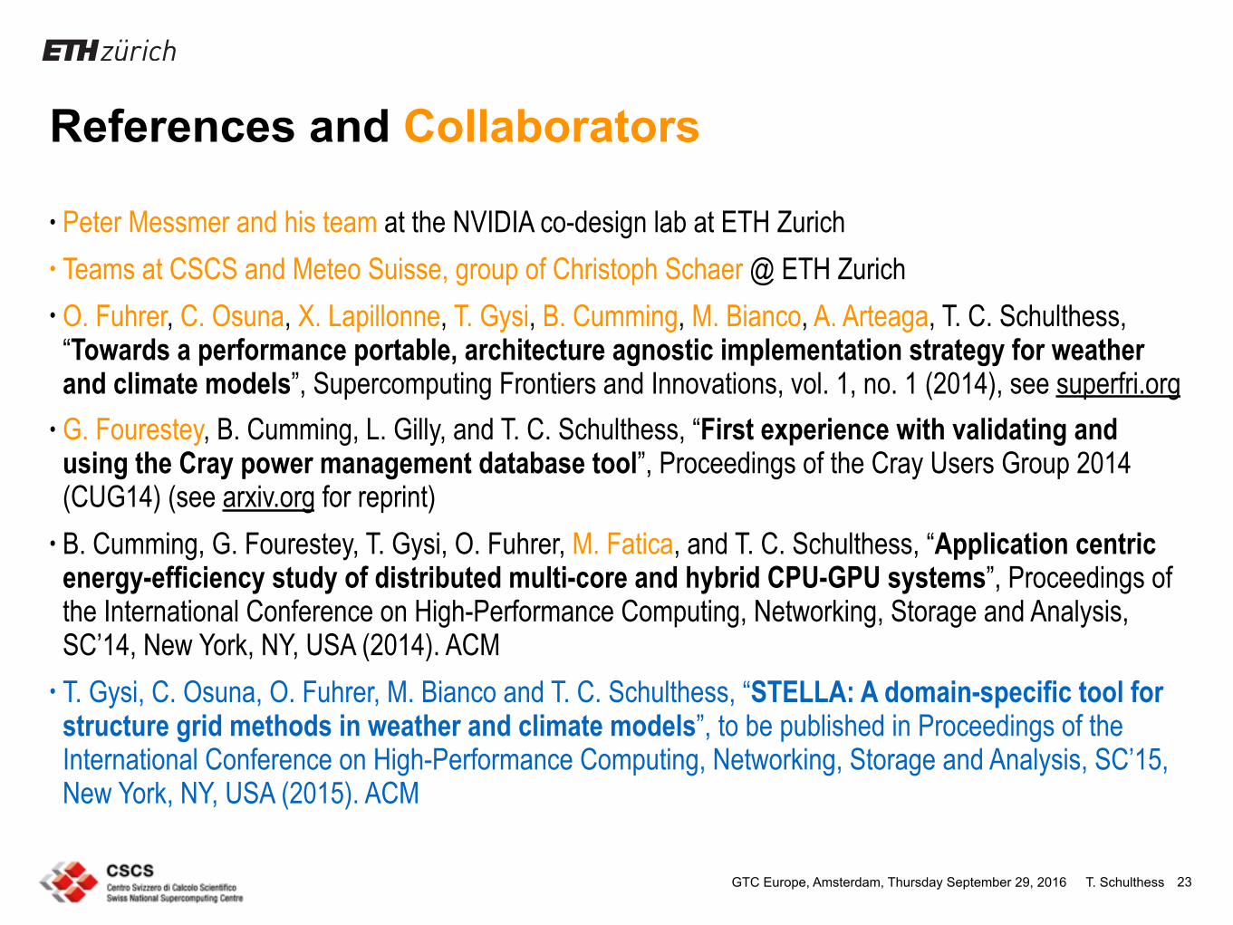
References and Collaborators
• Peter Messmer and his team at the NVIDIA co-design lab at ETH Zurich • Teams at CSCS and Meteo Suisse, group of Christoph Schaer @ ETH Zurich • O. Fuhrer, C. Osuna, X. Lapillonne, T. Gysi, B. Cumming, M. Bianco, A. Arteaga, T. C. Schulthess, “Towards a performance portable, architecture agnostic implementation strategy for weather and climate models”, Supercomputing Frontiers and Innovations, vol. 1, no. 1 (2014), see superfri.org
• G. Fourestey, B. Cumming, L. Gilly, and T. C. Schulthess, “First experience with validating and using the Cray power management database tool”, Proceedings of the Cray Users Group 2014 (CUG14) (see arxiv.org for reprint)
• B. Cumming, G. Fourestey, T. Gysi, O. Fuhrer, M. Fatica, and T. C. Schulthess, “Application centric energy-efficiency study of distributed multi-core and hybrid CPU-GPU systems”, Proceedings of the International Conference on High-Performance Computing, Networking, Storage and Analysis, SC’14, New York, NY, USA (2014). ACM
• T. Gysi, C. Osuna, O. Fuhrer, M. Bianco and T. C. Schulthess, “STELLA: A domain-specific tool for structure grid methods in weather and climate models”, to be published in Proceedings of the International Conference on High-Performance Computing, Networking, Storage and Analysis, SC’15, New York, NY, USA (2015). ACM
T. Schulthess17th Workshop on HPC in Meteorology @ ECMWF, Reading, Wednesday October 26, 2016
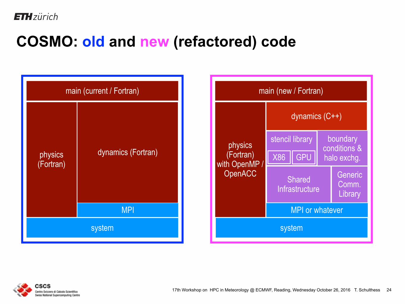
COSMO: old and new (refactored) code
24
main (current / Fortran)
physics (Fortran)
dynamics (Fortran)
MPI
system
main (new / Fortran)
physics (Fortran)
with OpenMP / OpenACC
dynamics (C++)
MPI or whatever
system
Generic Comm. Library
boundary conditions & halo exchg.
stencil library
X86 GPU
Shared Infrastructure

T. SchulthessGTC Europe, Amsterdam, Thursday September 29, 2016 25
Physical model
Algorithmic description
Compilation
Computer
Imperative codelap(i,j,k) = –4.0 * data(i,j,k) + data(i+1,j,k) + data(i-1,j,k) + data(i,j+1,k) + data(i,j-1,k);
Domain science & applied mathematics
Computer engineering
370 NATURE PHYSICS | VOL 11 | MAY 2015 | www.nature.com/naturephysics
COMMENTARY | FOCUS
Whereas this long-term sustained exponential growth had profound impact on the productivity of scientists and opened many new avenues in physics research, not all types of problems in scientific computing have seen the same performance improvements. For example, the sustained performance of climate codes, as documented by the European Centre for Medium-Range Weather Forecasts (ECMWF) over approximately the same period as the Top500 project, has improved only by a factor of 100 per decade (Peter Bauer, manuscript in preparation). This is still an exponential growth, but it demonstrates the significant decrease in efficiency for software applications in some fields. This is more important, as meteorological and climate simulations have been around since the dawn of modern computing1. They rely on complex, but typically well-engineered computer codes that have been designed to run on the top supercomputing systems. If experts use computers inefficiently, what does this say about the applications developed by regular researchers?
In this Commentary, I discuss state-of-the-art programming and parallelization in physics today. I try to analyse the challenges in writing efficient scientific software and examine possible ways in which physicists can deal with the rapidly increasing complexity of computer architectures. To do so it is important to first recall the main uses of computing in physics.
Imperative code
Compilation
Physical modelMathematical description
Algorithmic description
Computer
Domain science and applied mathematics
Computer engineering
= − ∇p + ρg − 2Ω×(ρv) + F
= − (cpd /cvdp∇· v + (cpd /cvd−1)Qh
= p· +Qh
= − ∇ · Fv − (Il + I f)= ∇ · (P l,f + F l,f) + Il,f
= p[Rd (1+(Rυ/Rd−1) qυ− q l−qf)T ]−1
ODSLMN ± GDWDLMNGDWDLMNGDWDLMNGDWDLMNGDWDLMN
Wind ρv·
Pressure p·
Water ρq· υ
ρq· l,f
Density ρ
Temperature ρcpd T·
Figure 1 | Traditional computational science workflow. A physical model (of the atmosphere, for instance) is first translated into mathematical equations (here, non-hydrostatic compressible Euler equations), which in turn are solved with algorithms (such as finite differences on a structured grid), implemented in a program (for example, stencil code), and subsequently compiled into machine code that executes on a canonical computer architecture. The green line marks the separation of work. The physical model image is adapted from ref. 9, NPG. The supercomputer image © British Crown Copyright, The Met Office / Science Photo Library.
Predictions and data analysisLong before the advent of modern computing, modelling and simulation were used in physics in two ways. The first and best known (which we call the traditional way) is the use of computers to solve challenging theoretical problems that have no known analytical solution. In this case, the theory is well understood and the governing equations are solved numerically with elaborate computational methods to make quantitative and verifiable predictions. Sometimes the numerical solution of a theoretical problem may lead to new insights in its own right, as was the case with the discovery of the fluctuation theorem2. This was an argument for defining computer simulations as a third, independent pillar of science, complementing theory and experiment3. For our purpose, this distinction is not necessary, as from a computational point of view we are still solving known equations. The simulations are carefully planned — that is, the mathematical analysis and algorithms are well known and the elaborate computer codes, as in the case of climate simulations, have been developed and optimized. Scientists, and physicists in particular, will not shy away from great efforts in using cutting-edge technologies to solve such problems, and they will use imperative programming languages such as C or FORTRAN with machine-level codes to squeeze every last bit of performance out of a computing system.
The second, and profoundly different, use is the analysis of experimental data with the help of modelling and simulations before the theory and governing equations are known. This is essentially what Johannes Kepler did when he analysed Tycho Brahe’s planetary orbit data with heliocentric elliptical models to discover the three famous laws that now carry his name — Newton’s theory of gravitation, which explains Kepler’s laws, came later. Scientists today use computers to rapidly prototype models, thereby assimilating in a matter of seconds or minutes many orders of magnitude more data than Kepler did in months of laborious manual computations. Along with the development of electronic computing came large experimental facilities, which significantly increased the importance of systematic exploratory tools for data analysis. This lead to a substantial improvement of mathematical algorithms over the past few decades, which, together with the emergence of social media on the World Wide Web, have made this exploratory use relevant to areas outside of natural sciences, for instance in economics and social sciences. These have, in turn, led to the argument that a fundamentally new, fourth paradigm of science is emerging: ‘data science’3. For our present purpose, however, this distinction is again not necessarily important. But, for this second exploratory use of modelling and simulation scientists use more descriptive programming languages like Python or Ruby, and they rely on existing libraries even if they are not optimized.
Scientists and computer engineersProgramming serves two complementary purposes: one is to specify the computation and the other is to manage computer resources. Most scientists are familiar with the former, whereas the latter is considered to be primarily the concern of computer engineers. The distinction is important as it allows a clear separation of concerns: scientists only need to know about the complexity of models and mathematics, and system engineers only need to focus on the complexity of the computer.
In this ideal case, the programming environment allows scientists to specify the computational tasks in terms of human-readable equations — descriptive programming — that are independent of the underlying system, which is portable across many platforms. The Python programming language, with its many associated libraries and tools, provides such an environment, but at the cost of performance. When the computation is big and has to be scaled, performance does matter. In this case scientists have the choice of algorithms
© 2015 Macmillan Publishers Limited. All rights reserved
Mathematical description
Schulthess, Nature Physics, vol 11, 369-373 (2015)

T. SchulthessGTC Europe, Amsterdam, Thursday September 29, 2016 26
Imperative code
Compilation
Computer
Domain science & applied mathematics
Computer engineering
Physical model
Mathematical description
Algorithmic description
Schulthess, Nature Physics, vol 11, 369-373 (2015)

T. SchulthessGTC Europe, Amsterdam, Thursday September 29, 2016 27
Physical model
Mathematical description
Algorithmic description
Imperative code
Compilation
Computer
Domain science & applied mathematics
Computer engineering Schulthess, Nature Physics, vol 11, 369-373 (2015)
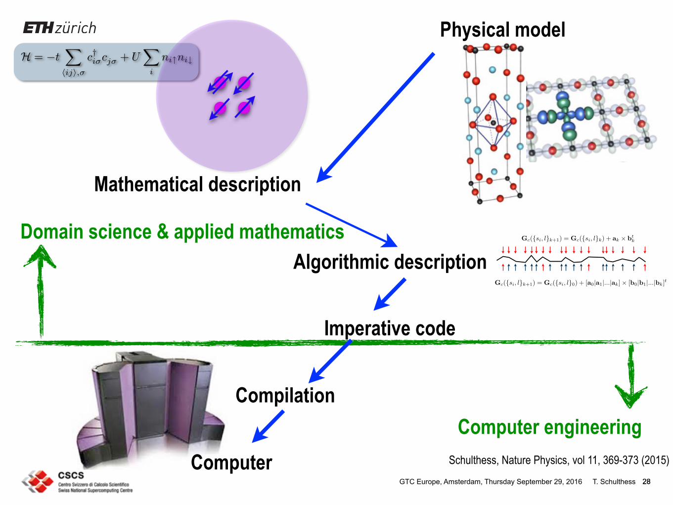
T. SchulthessGTC Europe, Amsterdam, Thursday September 29, 2016 28
Imperative code
Compilation
Computer
Domain science & applied mathematics
Computer engineering
Physical model
Mathematical description
H = −t!
⟨ij⟩,σ
c†iσcjσ + U!
i
ni↑ni↓
Algorithmic descriptionGc(si, lk+1) = Gc(si, l0) + [a0|a1|...|ak] × [b0|b1|...|bk]t
Gc(si, lk+1) = Gc(si, lk) + ak × btk
28
Schulthess, Nature Physics, vol 11, 369-373 (2015)

T. SchulthessGTC Europe, Amsterdam, Thursday September 29, 2016 29
Physical model
Algorithmic description
Imperative code
Compilation
lap(i,j,k) = –4.0 * data(i,j,k) + data(i+1,j,k) + data(i-1,j,k) + data(i,j+1,k) + data(i,j-1,k);
Domain science & applied mathematics
Computer engineering
370 NATURE PHYSICS | VOL 11 | MAY 2015 | www.nature.com/naturephysics
COMMENTARY | FOCUS
Whereas this long-term sustained exponential growth had profound impact on the productivity of scientists and opened many new avenues in physics research, not all types of problems in scientific computing have seen the same performance improvements. For example, the sustained performance of climate codes, as documented by the European Centre for Medium-Range Weather Forecasts (ECMWF) over approximately the same period as the Top500 project, has improved only by a factor of 100 per decade (Peter Bauer, manuscript in preparation). This is still an exponential growth, but it demonstrates the significant decrease in efficiency for software applications in some fields. This is more important, as meteorological and climate simulations have been around since the dawn of modern computing1. They rely on complex, but typically well-engineered computer codes that have been designed to run on the top supercomputing systems. If experts use computers inefficiently, what does this say about the applications developed by regular researchers?
In this Commentary, I discuss state-of-the-art programming and parallelization in physics today. I try to analyse the challenges in writing efficient scientific software and examine possible ways in which physicists can deal with the rapidly increasing complexity of computer architectures. To do so it is important to first recall the main uses of computing in physics.
Imperative code
Compilation
Physical modelMathematical description
Algorithmic description
Computer
Domain science and applied mathematics
Computer engineering
= − ∇p + ρg − 2Ω×(ρv) + F
= − (cpd /cvdp∇· v + (cpd /cvd−1)Qh
= p· +Qh
= − ∇ · Fv − (Il + I f)= ∇ · (P l,f + F l,f) + Il,f
= p[Rd (1+(Rυ/Rd−1) qυ− q l−qf)T ]−1
ODSLMN ± GDWDLMNGDWDLMNGDWDLMNGDWDLMNGDWDLMN
Wind ρv·
Pressure p·
Water ρq· υ
ρq· l,f
Density ρ
Temperature ρcpd T·
Figure 1 | Traditional computational science workflow. A physical model (of the atmosphere, for instance) is first translated into mathematical equations (here, non-hydrostatic compressible Euler equations), which in turn are solved with algorithms (such as finite differences on a structured grid), implemented in a program (for example, stencil code), and subsequently compiled into machine code that executes on a canonical computer architecture. The green line marks the separation of work. The physical model image is adapted from ref. 9, NPG. The supercomputer image © British Crown Copyright, The Met Office / Science Photo Library.
Predictions and data analysisLong before the advent of modern computing, modelling and simulation were used in physics in two ways. The first and best known (which we call the traditional way) is the use of computers to solve challenging theoretical problems that have no known analytical solution. In this case, the theory is well understood and the governing equations are solved numerically with elaborate computational methods to make quantitative and verifiable predictions. Sometimes the numerical solution of a theoretical problem may lead to new insights in its own right, as was the case with the discovery of the fluctuation theorem2. This was an argument for defining computer simulations as a third, independent pillar of science, complementing theory and experiment3. For our purpose, this distinction is not necessary, as from a computational point of view we are still solving known equations. The simulations are carefully planned — that is, the mathematical analysis and algorithms are well known and the elaborate computer codes, as in the case of climate simulations, have been developed and optimized. Scientists, and physicists in particular, will not shy away from great efforts in using cutting-edge technologies to solve such problems, and they will use imperative programming languages such as C or FORTRAN with machine-level codes to squeeze every last bit of performance out of a computing system.
The second, and profoundly different, use is the analysis of experimental data with the help of modelling and simulations before the theory and governing equations are known. This is essentially what Johannes Kepler did when he analysed Tycho Brahe’s planetary orbit data with heliocentric elliptical models to discover the three famous laws that now carry his name — Newton’s theory of gravitation, which explains Kepler’s laws, came later. Scientists today use computers to rapidly prototype models, thereby assimilating in a matter of seconds or minutes many orders of magnitude more data than Kepler did in months of laborious manual computations. Along with the development of electronic computing came large experimental facilities, which significantly increased the importance of systematic exploratory tools for data analysis. This lead to a substantial improvement of mathematical algorithms over the past few decades, which, together with the emergence of social media on the World Wide Web, have made this exploratory use relevant to areas outside of natural sciences, for instance in economics and social sciences. These have, in turn, led to the argument that a fundamentally new, fourth paradigm of science is emerging: ‘data science’3. For our present purpose, however, this distinction is again not necessarily important. But, for this second exploratory use of modelling and simulation scientists use more descriptive programming languages like Python or Ruby, and they rely on existing libraries even if they are not optimized.
Scientists and computer engineersProgramming serves two complementary purposes: one is to specify the computation and the other is to manage computer resources. Most scientists are familiar with the former, whereas the latter is considered to be primarily the concern of computer engineers. The distinction is important as it allows a clear separation of concerns: scientists only need to know about the complexity of models and mathematics, and system engineers only need to focus on the complexity of the computer.
In this ideal case, the programming environment allows scientists to specify the computational tasks in terms of human-readable equations — descriptive programming — that are independent of the underlying system, which is portable across many platforms. The Python programming language, with its many associated libraries and tools, provides such an environment, but at the cost of performance. When the computation is big and has to be scaled, performance does matter. In this case scientists have the choice of algorithms
© 2015 Macmillan Publishers Limited. All rights reserved
Mathematical description
Schulthess, Nature Physics, vol 11, 369-373 (2015)

T. SchulthessGTC Europe, Amsterdam, Thursday September 29, 2016 30
Algorithmic description
Imperative code
Compilation
lap(i,j,k) = –4.0 * data(i,j,k) + data(i+1,j,k) + data(i-1,j,k) + data(i,j+1,k) + data(i,j-1,k);
Domain science & applied mathematics
Computer engineering
370 NATURE PHYSICS | VOL 11 | MAY 2015 | www.nature.com/naturephysics
COMMENTARY | FOCUS
Whereas this long-term sustained exponential growth had profound impact on the productivity of scientists and opened many new avenues in physics research, not all types of problems in scientific computing have seen the same performance improvements. For example, the sustained performance of climate codes, as documented by the European Centre for Medium-Range Weather Forecasts (ECMWF) over approximately the same period as the Top500 project, has improved only by a factor of 100 per decade (Peter Bauer, manuscript in preparation). This is still an exponential growth, but it demonstrates the significant decrease in efficiency for software applications in some fields. This is more important, as meteorological and climate simulations have been around since the dawn of modern computing1. They rely on complex, but typically well-engineered computer codes that have been designed to run on the top supercomputing systems. If experts use computers inefficiently, what does this say about the applications developed by regular researchers?
In this Commentary, I discuss state-of-the-art programming and parallelization in physics today. I try to analyse the challenges in writing efficient scientific software and examine possible ways in which physicists can deal with the rapidly increasing complexity of computer architectures. To do so it is important to first recall the main uses of computing in physics.
Imperative code
Compilation
Physical modelMathematical description
Algorithmic description
Computer
Domain science and applied mathematics
Computer engineering
= − ∇p + ρg − 2Ω×(ρv) + F
= − (cpd /cvdp∇· v + (cpd /cvd−1)Qh
= p· +Qh
= − ∇ · Fv − (Il + I f)= ∇ · (P l,f + F l,f) + Il,f
= p[Rd (1+(Rυ/Rd−1) qυ− q l−qf)T ]−1
ODSLMN ± GDWDLMNGDWDLMNGDWDLMNGDWDLMNGDWDLMN
Wind ρv·
Pressure p·
Water ρq· υ
ρq· l,f
Density ρ
Temperature ρcpd T·
Figure 1 | Traditional computational science workflow. A physical model (of the atmosphere, for instance) is first translated into mathematical equations (here, non-hydrostatic compressible Euler equations), which in turn are solved with algorithms (such as finite differences on a structured grid), implemented in a program (for example, stencil code), and subsequently compiled into machine code that executes on a canonical computer architecture. The green line marks the separation of work. The physical model image is adapted from ref. 9, NPG. The supercomputer image © British Crown Copyright, The Met Office / Science Photo Library.
Predictions and data analysisLong before the advent of modern computing, modelling and simulation were used in physics in two ways. The first and best known (which we call the traditional way) is the use of computers to solve challenging theoretical problems that have no known analytical solution. In this case, the theory is well understood and the governing equations are solved numerically with elaborate computational methods to make quantitative and verifiable predictions. Sometimes the numerical solution of a theoretical problem may lead to new insights in its own right, as was the case with the discovery of the fluctuation theorem2. This was an argument for defining computer simulations as a third, independent pillar of science, complementing theory and experiment3. For our purpose, this distinction is not necessary, as from a computational point of view we are still solving known equations. The simulations are carefully planned — that is, the mathematical analysis and algorithms are well known and the elaborate computer codes, as in the case of climate simulations, have been developed and optimized. Scientists, and physicists in particular, will not shy away from great efforts in using cutting-edge technologies to solve such problems, and they will use imperative programming languages such as C or FORTRAN with machine-level codes to squeeze every last bit of performance out of a computing system.
The second, and profoundly different, use is the analysis of experimental data with the help of modelling and simulations before the theory and governing equations are known. This is essentially what Johannes Kepler did when he analysed Tycho Brahe’s planetary orbit data with heliocentric elliptical models to discover the three famous laws that now carry his name — Newton’s theory of gravitation, which explains Kepler’s laws, came later. Scientists today use computers to rapidly prototype models, thereby assimilating in a matter of seconds or minutes many orders of magnitude more data than Kepler did in months of laborious manual computations. Along with the development of electronic computing came large experimental facilities, which significantly increased the importance of systematic exploratory tools for data analysis. This lead to a substantial improvement of mathematical algorithms over the past few decades, which, together with the emergence of social media on the World Wide Web, have made this exploratory use relevant to areas outside of natural sciences, for instance in economics and social sciences. These have, in turn, led to the argument that a fundamentally new, fourth paradigm of science is emerging: ‘data science’3. For our present purpose, however, this distinction is again not necessarily important. But, for this second exploratory use of modelling and simulation scientists use more descriptive programming languages like Python or Ruby, and they rely on existing libraries even if they are not optimized.
Scientists and computer engineersProgramming serves two complementary purposes: one is to specify the computation and the other is to manage computer resources. Most scientists are familiar with the former, whereas the latter is considered to be primarily the concern of computer engineers. The distinction is important as it allows a clear separation of concerns: scientists only need to know about the complexity of models and mathematics, and system engineers only need to focus on the complexity of the computer.
In this ideal case, the programming environment allows scientists to specify the computational tasks in terms of human-readable equations — descriptive programming — that are independent of the underlying system, which is portable across many platforms. The Python programming language, with its many associated libraries and tools, provides such an environment, but at the cost of performance. When the computation is big and has to be scaled, performance does matter. In this case scientists have the choice of algorithms
© 2015 Macmillan Publishers Limited. All rights reserved
Mathematical description
Physical model
Schulthess, Nature Physics, vol 11, 369-373 (2015)
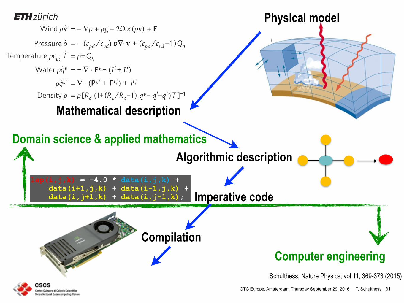
T. SchulthessGTC Europe, Amsterdam, Thursday September 29, 2016 31
Physical model
Algorithmic description
Imperative code
Compilation
lap(i,j,k) = –4.0 * data(i,j,k) + data(i+1,j,k) + data(i-1,j,k) + data(i,j+1,k) + data(i,j-1,k);
Domain science & applied mathematics
Computer engineering
370 NATURE PHYSICS | VOL 11 | MAY 2015 | www.nature.com/naturephysics
COMMENTARY | FOCUS
Whereas this long-term sustained exponential growth had profound impact on the productivity of scientists and opened many new avenues in physics research, not all types of problems in scientific computing have seen the same performance improvements. For example, the sustained performance of climate codes, as documented by the European Centre for Medium-Range Weather Forecasts (ECMWF) over approximately the same period as the Top500 project, has improved only by a factor of 100 per decade (Peter Bauer, manuscript in preparation). This is still an exponential growth, but it demonstrates the significant decrease in efficiency for software applications in some fields. This is more important, as meteorological and climate simulations have been around since the dawn of modern computing1. They rely on complex, but typically well-engineered computer codes that have been designed to run on the top supercomputing systems. If experts use computers inefficiently, what does this say about the applications developed by regular researchers?
In this Commentary, I discuss state-of-the-art programming and parallelization in physics today. I try to analyse the challenges in writing efficient scientific software and examine possible ways in which physicists can deal with the rapidly increasing complexity of computer architectures. To do so it is important to first recall the main uses of computing in physics.
Imperative code
Compilation
Physical modelMathematical description
Algorithmic description
Computer
Domain science and applied mathematics
Computer engineering
= − ∇p + ρg − 2Ω×(ρv) + F
= − (cpd /cvdp∇· v + (cpd /cvd−1)Qh
= p· +Qh
= − ∇ · Fv − (Il + I f)= ∇ · (P l,f + F l,f) + Il,f
= p[Rd (1+(Rυ/Rd−1) qυ− q l−qf)T ]−1
ODSLMN ± GDWDLMNGDWDLMNGDWDLMNGDWDLMNGDWDLMN
Wind ρv·
Pressure p·
Water ρq· υ
ρq· l,f
Density ρ
Temperature ρcpd T·
Figure 1 | Traditional computational science workflow. A physical model (of the atmosphere, for instance) is first translated into mathematical equations (here, non-hydrostatic compressible Euler equations), which in turn are solved with algorithms (such as finite differences on a structured grid), implemented in a program (for example, stencil code), and subsequently compiled into machine code that executes on a canonical computer architecture. The green line marks the separation of work. The physical model image is adapted from ref. 9, NPG. The supercomputer image © British Crown Copyright, The Met Office / Science Photo Library.
Predictions and data analysisLong before the advent of modern computing, modelling and simulation were used in physics in two ways. The first and best known (which we call the traditional way) is the use of computers to solve challenging theoretical problems that have no known analytical solution. In this case, the theory is well understood and the governing equations are solved numerically with elaborate computational methods to make quantitative and verifiable predictions. Sometimes the numerical solution of a theoretical problem may lead to new insights in its own right, as was the case with the discovery of the fluctuation theorem2. This was an argument for defining computer simulations as a third, independent pillar of science, complementing theory and experiment3. For our purpose, this distinction is not necessary, as from a computational point of view we are still solving known equations. The simulations are carefully planned — that is, the mathematical analysis and algorithms are well known and the elaborate computer codes, as in the case of climate simulations, have been developed and optimized. Scientists, and physicists in particular, will not shy away from great efforts in using cutting-edge technologies to solve such problems, and they will use imperative programming languages such as C or FORTRAN with machine-level codes to squeeze every last bit of performance out of a computing system.
The second, and profoundly different, use is the analysis of experimental data with the help of modelling and simulations before the theory and governing equations are known. This is essentially what Johannes Kepler did when he analysed Tycho Brahe’s planetary orbit data with heliocentric elliptical models to discover the three famous laws that now carry his name — Newton’s theory of gravitation, which explains Kepler’s laws, came later. Scientists today use computers to rapidly prototype models, thereby assimilating in a matter of seconds or minutes many orders of magnitude more data than Kepler did in months of laborious manual computations. Along with the development of electronic computing came large experimental facilities, which significantly increased the importance of systematic exploratory tools for data analysis. This lead to a substantial improvement of mathematical algorithms over the past few decades, which, together with the emergence of social media on the World Wide Web, have made this exploratory use relevant to areas outside of natural sciences, for instance in economics and social sciences. These have, in turn, led to the argument that a fundamentally new, fourth paradigm of science is emerging: ‘data science’3. For our present purpose, however, this distinction is again not necessarily important. But, for this second exploratory use of modelling and simulation scientists use more descriptive programming languages like Python or Ruby, and they rely on existing libraries even if they are not optimized.
Scientists and computer engineersProgramming serves two complementary purposes: one is to specify the computation and the other is to manage computer resources. Most scientists are familiar with the former, whereas the latter is considered to be primarily the concern of computer engineers. The distinction is important as it allows a clear separation of concerns: scientists only need to know about the complexity of models and mathematics, and system engineers only need to focus on the complexity of the computer.
In this ideal case, the programming environment allows scientists to specify the computational tasks in terms of human-readable equations — descriptive programming — that are independent of the underlying system, which is portable across many platforms. The Python programming language, with its many associated libraries and tools, provides such an environment, but at the cost of performance. When the computation is big and has to be scaled, performance does matter. In this case scientists have the choice of algorithms
© 2015 Macmillan Publishers Limited. All rights reserved
Mathematical description
Schulthess, Nature Physics, vol 11, 369-373 (2015)

T. SchulthessSimons Foundation Lectures, Frontier of Data Science, New York, Wednesday, May 11, 2016 32
Science applications using a descriptive and dynamic developer environment
Physical modelMathematical description
Algorithmic description
Imperative code
Architecture 1
Compiler frontend
Optimisation / low-level libraries / runtime
Architecture specific backends
Architecture 2 Architecture N…
Multi-disciplinary co-design of tools, libraries, programming environment
dynamic environmentfor model develop.
tools forhigh-performance
scientific computing
Schulthess, Nature Physics, vol 11, 369-373 (2015)
iPython/notebookJUPYTER

T. Schulthess17th Workshop on HPC in Meteorology @ ECMWF, Reading, Wednesday October 26, 2016
The good news
33
C++ 11, 14, HPX-3, … 17, 20, …
C++ standard is evolving quickly and implementations follow!

T. Schulthess17th Workshop on HPC in Meteorology @ ECMWF, Reading, Wednesday October 26, 2016 34
Who will pay for the implementation of Fortran, OpenACC, OpenMP, …?

T. Schulthess17th Workshop on HPC in Meteorology @ ECMWF, Reading, Wednesday October 26, 2016 35
Source: Andy Keane @ ISC’10
for 8 GPUs, or $16k a piece
$500,000,000 $2,000,000,000
$13,000

T. Schulthess17th Workshop on HPC in Meteorology @ ECMWF, Reading, Wednesday October 26, 2016 36

T. Schulthess17th Workshop on HPC in Meteorology @ ECMWF, Reading, Wednesday October 26, 2016 37
Areas of interest include (but are not limited to):
- Theuseofadvancedcomputingsystemsforlarge-scalescientificapplications- Implementationstrategiesforscienceapplicationsinenergy-efficientcomputing architectures- Domain-specific,languages,librariesorframeworks- Theintegrationoflarge-scaleexperimentalandobservationalscientificdataandhigh- performance data analytics and computing- Bestpracticesforsustainablesoftwaredevelopmentandscientificapplication development
Committee ChairsJackWells(OakRidgeNationalLaboratory,USA)TorstenHoefler(ETHZurich,Switzerland)
Submission GuidelinesWeinvitepapersof5-10pagesinlength,whichwillberevieweddoubleblind.Fullsubmis-sionsguidelinescanbefoundatwww.pasc17.org.
-Submissionsclose:12 December 2016-Firstreviewnotification:31 January 2017-Revisedsubmissionsclose:1 March 2017-Finalacceptancenotification:11 April 2017
Conference Participation and ProceedingsAcceptedmanuscriptswillbepublished in the ACM Digital Libraryonthefirstdayoftheconference.Authorswillbegiven30-minutepresentationslotsattheconference,groupedintopicallyfocused,parallelsessions.
Post-Conference Journal SubmissionFollowingtheconference,authorswillhavetheopportunity to develop their papers for publication in a relevant, computationally focused, domain-specific journal.
Authorsthusstandtobenefitfromtherapidandbroaddisseminationofresultsaffordedbytheconferencevenueandassociatedproceedings,and,fromtheimpactassociatedwithpublicationinahigh-qualityscientificjournal.
The Platform for Advanced Scientific Computing (PASC) invites submissions for the PASC17 Conference, co-sponsored by the Association for Computing Machinery (ACM) and SIGHPC, which will be held at the Palazzo dei Congressi in Lugano, Switzerland, from June 26 to 28, 2017.
PASC17isaninterdisciplinaryeventinhighperformancecomputingthatbringstogetherdomainscience,appliedmathematicsandcomputerscience-wherecomputerscienceisfocusedonenablingtherealizationofscientificcomputation.
Wearesolicitinghigh-qualitycontributionsoforiginalresearchrelatingtohighperformancecomputingineightdomain-specifictracks:
pasc17.pasc-conference.org
CLIMATE &WEATHER
SOLID EARTH DYNAMICS
LIFE SCIENCES
CHEMISTRY&MATERIALS
PHYSICS
COMPUTER SCIENCE & APPLIED MATHEMATICS
ENGINEERING
EMERGING DOMAINS (SPECIAL TOPIC: PRECISION MEDICINE)
Call for Papers