Embed Size (px)
Citation preview
Excel 2007/2010 for Researchers
Jamie DeCoster Institute for Social Science Research
University of Alabama
September 7, 2010
I’d like to thank Joe Chandler for comments made on an earlier version of these notes. If you wish to cite the contents of this document, the APA reference for them would be
DeCoster, J. (2010). Excel 2007/2010 for Researchers. Retrieved (month, day, and year you downloaded this file, without the parentheses) from http://www.stat-help.com/notes.html
All rights to this document are reserved
Table of Contents
Introduction ..................................................................................................................................... 1 Parts of an Excel Worksheet ........................................................................................................ 1
Editing and selecting ....................................................................................................................... 4 Entering and Editing Data ........................................................................................................... 4 Selecting Cells ............................................................................................................................. 5 Inserting and Deleting Rows and Columns ................................................................................. 6 Copy, Cut, and Paste.................................................................................................................... 6 Search and Replace ...................................................................................................................... 7 Data Validation ............................................................................................................................ 8
Altering the Display ...................................................................................................................... 11 Changing Text Attributes .......................................................................................................... 11 Changing the Size of Rows and Columns ................................................................................. 14 Simultaneously Viewing Different Parts of One Spreadsheet................................................... 16 Hiding and Filtering................................................................................................................... 18 Sorting Data ............................................................................................................................... 21
Formulas ....................................................................................................................................... 22 Formulas Without Functions ..................................................................................................... 22 Formulas With Functions .......................................................................................................... 23 Descriptions of Specific Functions ............................................................................................ 24 Nested Functions ....................................................................................................................... 26 Copy and Paste with Formulas .................................................................................................. 28 Goal Seek ................................................................................................................................... 29
Autofill .......................................................................................................................................... 31 Using the Fill Handle ................................................................................................................. 31 Copying Cell Contents............................................................................................................... 31 Incrementing Cell Values .......................................................................................................... 32 Formulas .................................................................................................................................... 33
Graphing data ................................................................................................................................ 34 Pie Charts ................................................................................................................................... 34 Column charts, bar charts and line charts .................................................................................. 34 Scatterplots ................................................................................................................................ 36 Customizing Charts ................................................................................................................... 37
Importing and Exporting Files ...................................................................................................... 38 Importing Data from a Word Processor .................................................................................... 38 Importing Data from SPSS or SAS ........................................................................................... 40 Exporting Data to a Word Processor ......................................................................................... 40 Exporting Data to SPSS or SAS ................................................................................................ 40
The Analysis Toolpak ................................................................................................................... 42 Installation ................................................................................................................................. 42 Analysis Input and Output ......................................................................................................... 42 Descriptive Statistics ................................................................................................................. 43 Inferential Statistics ................................................................................................................... 43 Random Number Generation ..................................................................................................... 48
1
1
INTRODUCTION In these notes we hope to provide a basic introduction to Microsoft Excel from the perspective of a researcher. Excel is a versatile and often overlooked program, and can be used to help a researcher at several different points in the scientific process. You can use Excel for:
• Entering the data from a study. Excel is designed to store information in a tabular format, which is perfect for creating a data set for analysis. It also contains a number of functions to make data entry easier and more accurate.
• Performing calculations. Excel’s formulas allow you to easily perform a broad range of mathematical calculations. These calculations can be based on the values entered into particular cells of the spreadsheet, which enables you to quickly see how changing the entry might affect the result of the equation.
• Analyzing data. Excel has the ability to perform t-tests, correlation, regression, and ANOVA. It also has built-in functions that can provide you with the p-values of all of the most commonly used statistics, including Z, t, F, and chi-square.
• Graphing. Excel can make a wide variety of graphs that can be copied and pasted into word processing documents and presentations.
• Exporting data sets. If you want perform your analyses in a more advanced statistical program, such as SPSS or SAS, Excel can save your tables in a format that can be read by these programs very easily.
• Randomization. Excel has a set of functions that allow you to generate random numbers with a wide variety of characteristics. These can be very useful if you want to randomly assigning subjects to conditions within an experiment.
One of its greatest features is that all of these things can be done without any complicated programming. Excel also has the ability for you to create much more powerful functions, if you want to make use of either its array functions or if you are interested in doing some of your own programming in VBA (visual basic for applications). In these notes, however, we will stick to the basic functions that come pre-programmed in Excel. Parts of an Excel Worksheet Figure 1 below graphically illustrates the parts of an Excel spreadsheet. With Office 2007, Microsoft has moved from the familiar menu-driven interface to a new tabbed ribbon interface. In this document we will explain how to use Excel functions using this new interface. If you are working with an earlier version of Excel, we have a different set of notes entitled "Excel 2003 for Researchers" that will explain how to use Excel using the menus. If you are working with Office 2007 but would prefer to use the menu-driven interface from Office 2003, you can purchase a relatively cheap program from http://www.addintools.com that will replace the tabbed ribbon with the original Office 2003 menus.

2
2
Row
Column
1
2
3
5
4
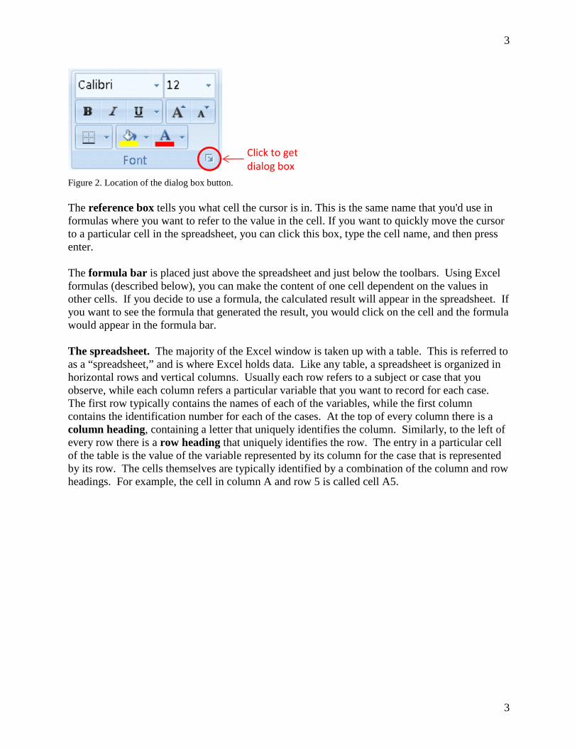
Figure 1. Parts of an Excel 2007 Spreadsheet. Number 1 is the tab menu, number 2 is where the command groups are displayed, number 3 is the reference box, number 4 is the formula bar, and number 5 is the spreadsheet. As you can see, the columns are vertical groups of cells, while rows are horizontal groups of cells. Tabs and command selections. At the top of the Excel window you will see a set of tabs, underneath of which are a set of command groups. Each command group will contain a number of different commands. Clicking on different tabs will change the command groups that are available. When describing how to do something in the ribbon interface, we will let you know where to find the command by telling you what tab it is in, what command group it is in, and finally the name of the specific command. We will do this using the following format. Tab Command group Command Sometimes an action doesn't have a specific button associated with it. Instead you have to find the appropriate command group and then click the little box in the lower-right hand corner to get the command group dialog box, illustrated in Figure 2 below. In this case we'll say "dialog box" instead of giving you a specific command.
3
3
Figure 2. Location of the dialog box button. The reference box tells you what cell the cursor is in. This is the same name that you'd use in formulas where you want to refer to the value in the cell. If you want to quickly move the cursor to a particular cell in the spreadsheet, you can click this box, type the cell name, and then press enter. The formula bar is placed just above the spreadsheet and just below the toolbars. Using Excel formulas (described below), you can make the content of one cell dependent on the values in other cells. If you decide to use a formula, the calculated result will appear in the spreadsheet. If you want to see the formula that generated the result, you would click on the cell and the formula would appear in the formula bar. The spreadsheet. The majority of the Excel window is taken up with a table. This is referred to as a “spreadsheet,” and is where Excel holds data. Like any table, a spreadsheet is organized in horizontal rows and vertical columns. Usually each row refers to a subject or case that you observe, while each column refers a particular variable that you want to record for each case. The first row typically contains the names of each of the variables, while the first column contains the identification number for each of the cases. At the top of every column there is a column heading, containing a letter that uniquely identifies the column. Similarly, to the left of every row there is a row heading that uniquely identifies the row. The entry in a particular cell of the table is the value of the variable represented by its column for the case that is represented by its row. The cells themselves are typically identified by a combination of the column and row headings. For example, the cell in column A and row 5 is called cell A5.
Click to get dialog box
4
4
EDITING AND SELECTING Entering and Editing Data Once you have opened an Excel spreadsheet, the first thing you need to do is to enter some data for it to work on. Entering data in Excel is a very easy task. All you need to do is click the specific cell that you want to edit, and then type in what you want the contents of that cell to be. You can then press the Tab key to move to the next cell to the right, or the Enter key to move to the next cell down. This allows you to enter your data very quickly without ever having to use the mouse. You can press Alt-Enter if you want to put a carriage return inside a cell entry. If you type an entry that is longer than the boundaries of the cell, your entry will overlap any empty cells to the right of the one you are editing. This does not actually place any information in these cells – Excel simply uses the unused space for display. If the cell to the right of the one you are editing contains data, then Excel will only display whatever characters fit in the established boundaries of the cell. The information is not lost, but it cannot be seen directly in the spreadsheet. You can see the full contents in the formula bar if you select the cell. Later on we will discuss ways you can have Excel display the full entry, such as by increasing the width of the cell or by using text wrapping. If you want to overwrite the contents of a cell that you’ve already entered, you just click on the cell and start typing. Your new entry will overwrite any data that was originally in the cell. If you want to edit the contents of a cell, you double-click the cell. Optionally, you can click the cell once to select it, and then click the place in the formula bar where you want to begin editing. This is most useful if the cell entry is very long, since you can specify exactly where you want the editing cursor to be placed. Anything you type will be inserted into the cell entry at the point that the cursor is placed. You can move the cursor within the entry by pressing the left and right arrow keys. You can use the backspace and delete keys to delete single characters before and after the cursor, respectively. You can also press the home key to immediately move the cursor in front of the first character of the entry, and the end key to move the cursor after the last character of the entry. Most often you will move yourself through an Excel spreadsheet using the mouse and the arrow keys. However, spreadsheets can become very large, so there are some shortcut keys that allow you to move quickly through your document. Some of the ones you will likely use most often are:
• Home: moves you to the far left cell of the current line • End: moves you to the far right cell of the current line • Page Up: scrolls the spreadsheet up one page • Page Dn: scrolls the spreadsheet down one page • Ctrl-Home: immediately moves you to the upper-left cell in the spreadsheet • Ctrl-End: immediately moves you to the lower-right cell in the spreadsheet
You can also move the scroll bars on the bottom and right of the spreadsheet to quickly change the cells you are viewing.
5
5
Selecting Cells There are a number of times when you will want to select cells in Excel. Sometimes you will want to copy or move the contents of a cell to another place in the spreadsheet. Sometimes you will want to select a range of cells for Excel to use in a function or formula. Sometimes you will want to take a portion of an Excel table and copy it into a word-processing document or a web page. In every case you select cells in the same way. To select a single cell:
• Click the cell once. To select an entire column
• Click the column heading. To select several adjacent columns
• Click the column heading of the leftmost column you want to select and hold the button down.
• Move the mouse pointer to the rightmost column you want to select. • Release the button.
To select an entire row
• Click the row heading. To select several adjacent rows
• Click the row heading of the top row you want to select and hold the button down. • Move the mouse pointer to the bottom row you want to select. • Release the button.
To select the entire spreadsheet
• Click the empty grey box at the upper-left hand corner of the spreadsheet. You may alternatively click Ctrl-A.
To select a group of cells that are all next to each other on the same screen
• Click a cell in one of the corners and hold the button down. • Move the mouse pointer to the opposite corner. • Release the button.
To select a group of cells that are all next to each other but are spread across several screens
• Click the upper-left cell once. • Press Shift and click the lower-right cell.
To select a group of cells that are not next to each other
• Click the first cell. • Press Ctrl and click all of the remaining cells.
6
6
Inserting and Deleting Rows and Columns If you want to clear the values from a set of cells without actually removing the corresponding cells from the spreadsheet, you can simply select the cells and press the Delete key. If you want to alter what cells you actually have in your spreadsheet you will need to perform the following procedures. To insert a column in your spreadsheet
• Select the column to the right of where you want the new column placed. • Choose Home → Cells → Insert
To insert a row in your spreadsheet
• Select the row below where you want the new row to be placed. • Choose Home → Cells → Insert
To delete a column or row in your spreadsheet
• Select the column or row you want to delete. • Choose Home → Cells → Delete
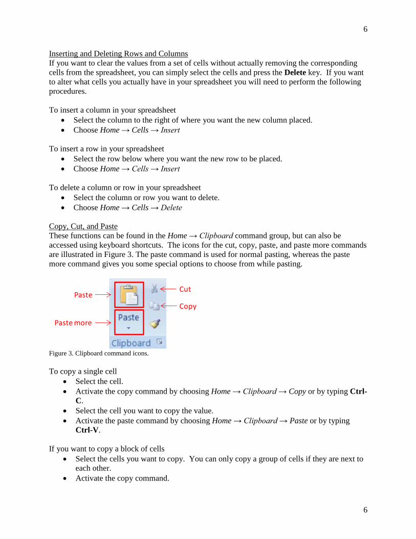
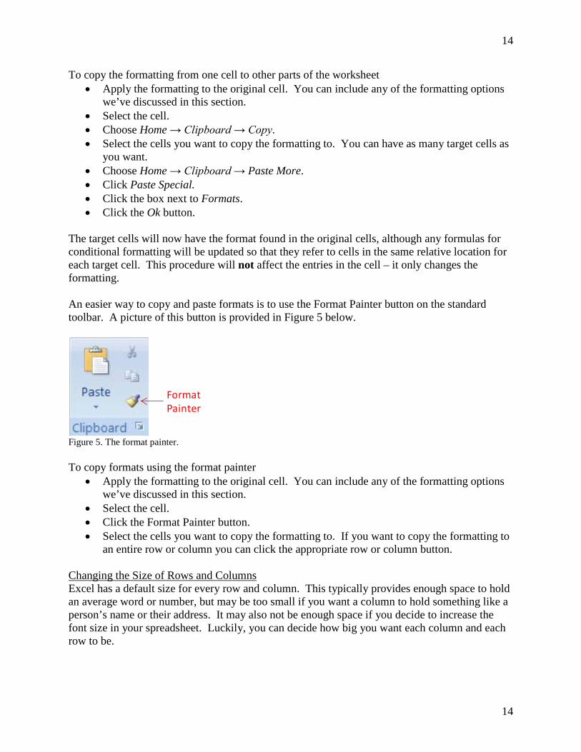
Copy, Cut, and Paste These functions can be found in the Home → Clipboard command group, but can also be accessed using keyboard shortcuts. The icons for the cut, copy, paste, and paste more commands are illustrated in Figure 3. The paste command is used for normal pasting, whereas the paste more command gives you some special options to choose from while pasting.
Cut
Copy
Paste more
Paste
Figure 3. Clipboard command icons. To copy a single cell
• Select the cell. • Activate the copy command by choosing Home → Clipboard → Copy or by typing Ctrl-
C. • Select the cell you want to copy the value. • Activate the paste command by choosing Home → Clipboard → Paste or by typing
Ctrl-V. If you want to copy a block of cells
• Select the cells you want to copy. You can only copy a group of cells if they are next to each other.
• Activate the copy command.
7
7
• Select the cell in the upper-left corner of the block where you want the cells to be copied. • Activate the paste command.
If you want to cut and paste a single cell
• Select the cell. • Activate the cut command by choosing Home → Clipboard → Cut or by typing Ctrl-X. • Select the cell you want to copy the value. • Activate the paste command.
If you want to cut and paste a block of cells
• Select the cells you want to cut. You can only cut and paste a group of cells if they are next to each other.
• Select the cut function. • Select the cell in the upper-left corner of the block where you want the cells to be pasted. • Select the paste function.
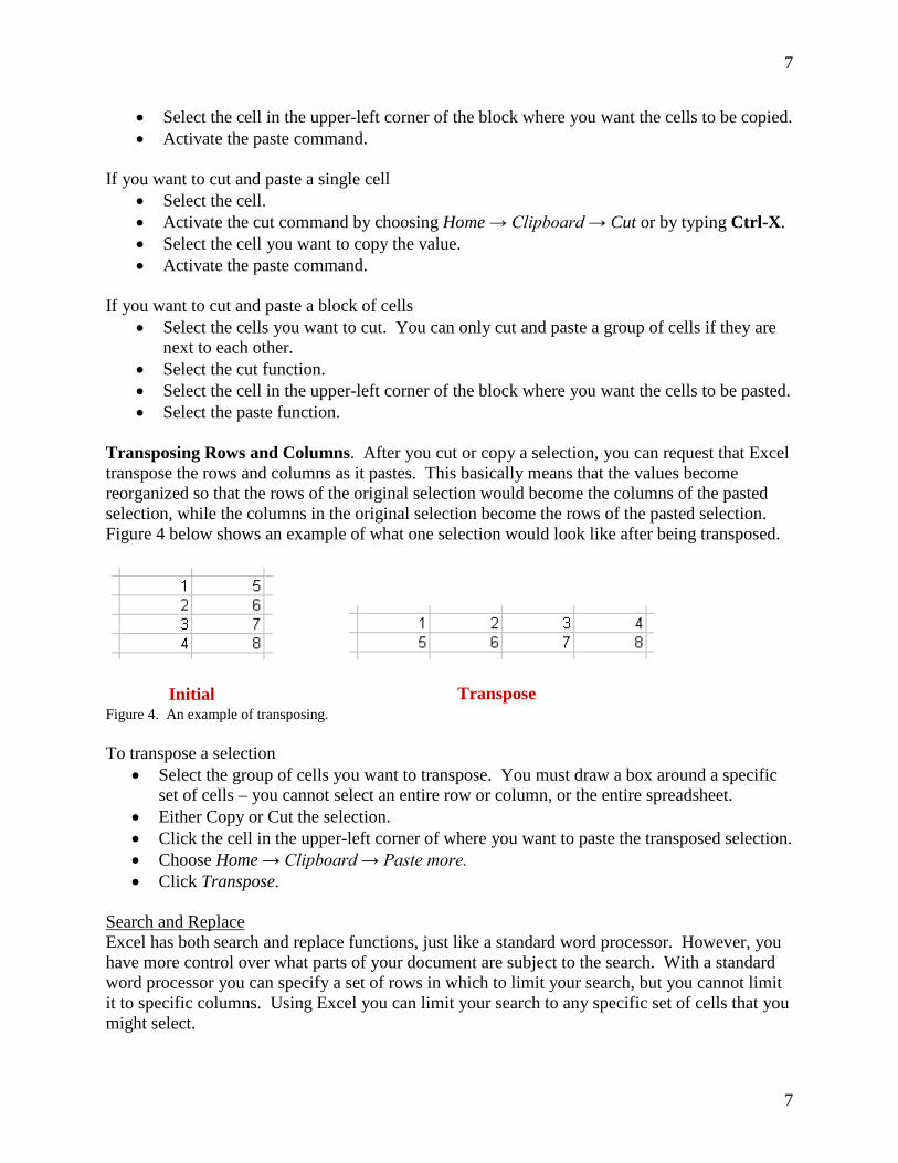
Transposing Rows and Columns. After you cut or copy a selection, you can request that Excel transpose the rows and columns as it pastes. This basically means that the values become reorganized so that the rows of the original selection would become the columns of the pasted selection, while the columns in the original selection become the rows of the pasted selection. Figure 4 below shows an example of what one selection would look like after being transposed. Figure 4. An example of transposing. To transpose a selection
• Select the group of cells you want to transpose. You must draw a box around a specific set of cells – you cannot select an entire row or column, or the entire spreadsheet.
• Either Copy or Cut the selection. • Click the cell in the upper-left corner of where you want to paste the transposed selection. • Choose Home → Clipboard → Paste more. • Click Transpose.
Search and Replace Excel has both search and replace functions, just like a standard word processor. However, you have more control over what parts of your document are subject to the search. With a standard word processor you can specify a set of rows in which to limit your search, but you cannot limit it to specific columns. Using Excel you can limit your search to any specific set of cells that you might select.
Initial Transpose
8
8
To perform a search • Select the cells that you want searched. If you do not select any cells then Excel will
search the entire spreadsheet. • Press Ctrl-F or choose Home → Editing → Find & Select and then click Find. • Type the text that you want to find into the box below Find what: • Click the button labeled Find Next. • Excel will then locate the first instance of the text that you entered. If the first instance
was not the one you were looking for, you can continue clicking Find Next until you have found the entry you want.
To perform a search and replace
• Select the cells that you want searched. If you do not select any cells then Excel will search the entire spreadsheet.
• Press Ctrl-H or choose Home → Editing → Find & Select and then click Replace. • Type the old text in box below Find what: • Type the new text in the box below Replace with: • Click the button labeled Find Next. • Excel will move to the first instance of the text that you entered.
o If you want to replace that instance of the old text, click the button labeled Replace. Excel will then move to the next instance of the old text.
o If you do not want to replace that instance of the old text but wish to continue searching, click the button labeled Find Next. Excel will then move to the next instance of the old text.
o If you want Excel to go through the entire document and replace all instances of the old text with the new text without confirmation, click the button labeled Replace all.
o If you want to stop the search and replace, click the button labeled Close. Data Validation Using data validation, you can control what types of values can be entered into various areas of your spreadsheet. You can specify both the type of entry as well as the specific range of values that are acceptable. You can even limit the entries to a specific set of values, which can then be chosen through a drop-down menu. You can have Excel display a message of your choosing in a “tool tip” box as soon as a cell with data validation is selected. Typically you will have this message tell the user what types of values should be put into the cell, so they are not surprised by any data validation errors they might receive. The box is reasonably small and does not interfere with data entry. You can choose exactly how you want Excel to react when someone does try to enter an invalid value. You can force the user to change the value into something that is acceptable, or you can just have a warning box pop up to tell the person that their entry doesn’t fit inside the acceptable range. To turn on data validation for a set of cells
• Select the cells you want to validate.
9
9
• Choose Data → Data Tools → Data Validation. • Click the Settings tab to specify what values are acceptable. First you use the drop-down
menu to choose what type of data will be contained in the cells. You then specify what range of values of that type are acceptable. You can have this range be constant, or you can have it depend on the entries in other cells of the worksheet. In the latter case you just define the minimum and maximum values as worksheet cells instead of as specific values.
o If you want to turn off data validation you can select Any value. o If you want to restrict entries to be integers, you select Whole number. This will
disallow entries with letters and numbers with anything after the decimal point. o If you want to restrict entries to be numbers but want to allow fractions, you select
Decimal. This disallows entries having any non-numeric characters in them. You also have the option of specifying the range of acceptable values.
o If you want to restrict entries to a list of pre-defined values, you select List. Using list validation is more complicated than the other validation types, and so we will cover it in more detail below.
o If you want to restrict entries to be times or dates, you select Time or Date, respectively. You can also specify a range of acceptable times or dates.
o If you want to allow the entries to be text, you select Text length. This actually allows users to make any type of entry they want. However, you can control the size of the entries by specifying the minimum and maximum size for valid entries.
o By default, the box next to Ignore blank will be checked. This allows users of the spreadsheet skip entering values into this cell. If you want to force users to enter an acceptable value when they select the cell you can uncheck this box.
• Click the Input Message tab to define a tool-tip message you want displayed as soon as someone selects one of the validated cells. You will usually use this tell users what type of data should be put in the cell. The text you type into the box beneath Title will appear at the top of the message in bold, while the text you type into the box beneath Input message will be displayed below the title in a normal font. If you do not define either of these, Excel will not present a tool-tip message when users select one of the validated cells.
• Click the Error Alert tab to define how Excel reacts when someone enters an invalid value.
o In the drop-down menu below Style you define what type of message Excel will present when someone tries to enter invalid data. A Stop message forces users to change the entry to a valid form before
they can proceed. It gives them a Retry option, allowing them to edit their entry, and a Cancel option, which deletes the entry.
A Warning message pops up a window that asks if users want to make an invalid entry. Users can select Yes, the entry is left as it is. If they select No, they are allowed to edit their entry. If they select Cancel, the invalid entry is deleted.
An Information message pops up a window stating that the entry is invalid. Users can then select Ok, which leaves the entry as it is, or Cancel, which deletes it.
10
10
o In the remaining boxes you can customize the message that is presented to users when they make an invalid entry. The text you type into the box beneath Title will appear at the top of the message in bold, while the text you type into the box beneath Error message will be displayed below the title in a normal font. If you do not define either of these, Excel will present a default error message.
List validation lets you specify exactly what values are allowed in a set of cells. One of the nice things about this type of validation is that it gives people using the worksheet the option of choosing values from a pull-down menu instead of having to type them in manually. To use list validation
• Type the list of valid values into the worksheet somewhere outside the cells where you are actually entering your data.
• Select the cells you want to validate. • Choose Data → Data Tools → Data Validation • Click the Settings tab. • Choose List from the pull-down menu in the Allow box. • Click the small button on the right-hand side of the box below Source. • Select the cells containing the acceptable values. • Press the Enter key. • Check the box next to In-cell dropdown if you want your users to be able to choose
values from a pull-down menu. This does not prevent them from typing values in directly.
• Choose the desired settings from the Input Message and Error Alert tabs as described above.
• Click the OK button.
11
11
ALTERING THE DISPLAY Sometimes the way that Excel presents your spreadsheet doesn’t meet your needs. Luckily you can customize many different aspects of the display. Changing Text Attributes When choosing how the contents of a cell should be displayed, you should first consider the general type of information that the cell will hold. Excel has defined a number of default presentation styles depending on whether a cell contains words, a number, a date, a dollar amount, and so forth. For example, if you tell Excel that a given cell is meant to contain a dollar amount, it will automatically display it with a dollar sign in front and round the amount to two decimal places. To select the general type of information that a set of cells will hold
• Select the cells you want to define. You will usually want to select an entire column, since each column usually holds information of a single type.
• Click on the pull-down menu in the Home → Number command group. • Choose the type that you want.
If you want, you can customize the display even further. For example, you can choose how many decimal points to display in a number, the symbol for currency (such as $, ₤, or €), or the way dates should be displayed. To access these more detailed options
• Select the cells you want to define. • Choose Home → Number → Dialog box. • Choose the type that you want. • Customize the specific nature of the display by selecting options on the right of the list.
You have control over several other aspects of text appearance within your spreadsheet. You can change the size, font, and color of the text in any of the cells. You can have different styles in different parts of the spreadsheet. To change the appearance of text within a set of cells
• Select the cells you want to change. • Select the new text attributes you want the contents of those cells to have in the Home →
Font command group. You can also change the justification and orientation of the text within the cells. You can choose to have the text justified to the left, center, or right of the cell. You can choose to have the text run vertically or at an angle. You can also control whether text exceeding the cell width automatically wraps to the next line or whether it is hidden. To change the justification or orientation of a set of cells
• Select the cells you want to change. • Select the alignment and orientation options you want the contents of those cells to have
in the Home → Alignment command group.
12
12
Conditional Formatting. One nice feature of Excel is that you can have it make the appearance of a cell depend on the value it contains. This can be used to highlight values that may be of special interest. There are quick formatting options that can change the appearance of a cell depending on whether it has low, medium or high values. To use quick formatting
• Choose Home → Styles → Conditional Formatting. • Click Data Bars, Color Scales, or Icon Sets, depending on how you want the value of the
cell to be illustrated. Selecting Data Bars will put small bar charts in each cell, Color Scales will shade the background of the cell between two colors representing low and high values, and Icon Sets will put a different icon in each cell depending on whether the value is low, medium, or high.
• A window will pop up asking you to select the exact appearance of the Data Bars, Color Scales or Icon Sets. Click whichever one you want.
You can also have Excel apply a formatting type any time that the cell value meets a particular criterion. To create a conditional format based on the cell value
• Select the cells for which you want to define conditional formatting • Choose Home → Styles → Conditional Formatting. • Click Highlight Cell Rules or Top/Bottom Rules. Highlight Cell Rules will allow you to
apply special formatting to cells that meet a specific criterion. Top/Bottom Rules will allow you to apply special formatting to cells that have either high or low values relative to others you have selected.
• Identify the type of rule you want to apply in the first window that pops up. • Set the specific criterion and determine the way you want the identified cells formatted in
the second window that pops up. Finally, you can choose to have a conditional format applied whenever the value of a particular formula is true. The benefit of using a formula is that you have more flexibility when defining the condition under which the formatting will be applied. Using formulas, you can have the formatting of a cell dependent on the value of other cells in the spreadsheet, or on the location of the cell in the worksheet. To create a conditional format based on a formula
• Select the cells for which you want to define conditional formatting • Choose Home → Styles → Conditional Formatting. • Click New Rule. • Click Use a formula to determine which cells to format in the window that pops up. • Type the formula in the box next to Format values where this formula is true. Be sure to
start your formula with an equals sign. The formatting will be applied whenever this formula is true. See the section on formulas below for more details about how to write
13
13
formulas. If you want to make the formatting dependent on the value of the current cell in some way you will need to explicitly refer to the cell in your formula.
• Click the button labeled Format to define the conditional format. o Selections in the Font tab are used to define the size, style, and color of the text in
the cell. o Selections in the Border tab can be used to set a border around the cell. o Selections in the Patterns tab can be used to set the color and shading in the
background of the cell. Below are some example formulas that you might find useful.
• =ROW()=ODD(ROW()) o Applies a format to every other row of a spreadsheet. This can be used to add
shading to make a table easier to read when combined with a pattern. • =COLUMN()=ODD(COLUMN())
o Applies a format to every other column of a spreadsheet. This can be used to add shading to make a table easier to read when combined with a pattern.
• =(MOD(ROW(), 5) = 1) o Applies a format to every fifth row. This can be used to add lines separating your
rows into groups of five when combined with a border. • =$A1 < 60
o You would need to set this formula up in row 1 and then apply it to the remainder of the spreadsheet. It will make the formatting dependent on the value in the first column of each row. If you would apply this to the entire row, then the whole row would have the conditional format whenever the value in the first column was less than 60.
• =A1 > average($A1:$G1) o You would need to set this formula up in cell a1 and then apply it to the
remainder of the cells. This would apply the format to the cell if its mean was greater than the mean of the cells from column A to column G in that particular row.
Copying and Pasting Formats. You have several options if you want to apply a set of formats to a number of different cells. First, you can simply select all of the cells and then define the formatting. However, this may not work if you are interested in using conditional formats based on formulas. Often times such conditional formats should be slightly different depending on the cell that is being formatted. For example, let us say that we wanted to use a conditional format to highlight the entire row when the value in the first column was over 100. Since every single row would require a different formula (since each row would base its formatting on a different cell), we could not just select the entire spreadsheet and define our formula. This does not mean, however, that we have to define the formatting for each row separately. Instead, we could define the formatting for a single row and then copy the formatting to the other cells in the spreadsheet. Excel automatically updates any formulas when you copy them to new cells (see Copy and Paste with Formulas below), so the formatting for any given cell would depend on the value of the first cell in its own row.
14
14
To copy the formatting from one cell to other parts of the worksheet • Apply the formatting to the original cell. You can include any of the formatting options
we’ve discussed in this section. • Select the cell. • Choose Home → Clipboard → Copy. • Select the cells you want to copy the formatting to. You can have as many target cells as
you want. • Choose Home → Clipboard → Paste More. • Click Paste Special. • Click the box next to Formats. • Click the Ok button.
The target cells will now have the format found in the original cells, although any formulas for conditional formatting will be updated so that they refer to cells in the same relative location for each target cell. This procedure will not affect the entries in the cell – it only changes the formatting. An easier way to copy and paste formats is to use the Format Painter button on the standard toolbar. A picture of this button is provided in Figure 5 below.
FormatPainter
Figure 5. The format painter. To copy formats using the format painter
• Apply the formatting to the original cell. You can include any of the formatting options we’ve discussed in this section.
• Select the cell. • Click the Format Painter button. • Select the cells you want to copy the formatting to. If you want to copy the formatting to
an entire row or column you can click the appropriate row or column button. Changing the Size of Rows and Columns Excel has a default size for every row and column. This typically provides enough space to hold an average word or number, but may be too small if you want a column to hold something like a person’s name or their address. It may also not be enough space if you decide to increase the font size in your spreadsheet. Luckily, you can decide how big you want each column and each row to be.
15
15
To change the size of a row • Move the cursor to the line that is just below of the row heading. The cursor should
change to a horizontal bar with up and down arrows. • Click the mouse button. • Drag the cursor up or down to change the size of the row.
To change the size of a column
• Move the cursor to the line that is just to the right of the column heading. The cursor should change to a vertical bar with arrows to the left and right.
• Click the mouse button. • Drag the cursor to the left or to the right to change the size of the column.
You can also change the size of a row or column through the menus by choosing Home → Cells → Format and then clicking either Row Height or Column Width. In this case you must enter a specific height or width in terms of point size (72 points = 1 inch). It’s usually easier to just resize a single column using the mouse (as described above), while it’s better to use the menu selections if you want to precisely control the size. Autofitting. Excel can autofit rows and columns, meaning that the size is automatically selected so that it is just large enough to fit the largest entry that you have. To autofit one or more rows
• Select the rows you want to autofit. • Choose Home → Cells → Format. • Click Autofit Row Height
To autofit one or more columns
• Select the columns you want to autofit. • Choose Home → Cells → Format. • Click Autofit Column Width
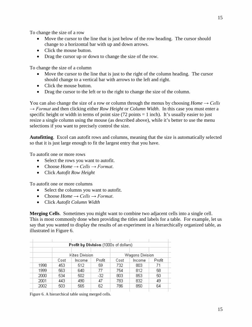
Merging Cells. Sometimes you might want to combine two adjacent cells into a single cell. This is most commonly done when providing the titles and labels for a table. For example, let us say that you wanted to display the results of an experiment in a hierarchically organized table, as illustrated in Figure 6.
Figure 6. A hierarchical table using merged cells.

16
16
As you can see, we have a single cell over the top of the table in which we put the title. In addition, you see that we merge three cells for each of the two division titles. Merging the cells for titles and labels makes it easier to keep the various elements in our table aligned. If we change the widths of one of the columns in the table, the title and the labels automatically change to keep them centered. If you merge cells that already contain information, the merged cell will take the value that was in the upper-left hand corner of the cells that you merged. Our example only merged cells horizontally, but it is perfectly possible to merge cells vertically as well. To merge a group of cells into a single cell
• Select the cells you want to merge. • Choose Home → Alignment → Merge & Center.
If you click the Merge & Center button while selecting a single cell that has already been merged, it will turn it back into a collection of individual cells. If you have any information in the merged cell, it will be placed in the cell that is in the upper-left hand corner of the group that composed the merged cell. Simultaneously Viewing Different Parts of One Spreadsheet. Usually your spreadsheet will take up more than a single screen. If you need to work with rows or columns that are not next to each other, it can grow tedious to constantly scroll back and forth. Luckily, Excel has two features that reduce the amount of scrolling you have to do. Freezing Panes. One of the most common reasons you might want to view different parts of a spreadsheet is to see the labels that you gave a row or column at the same time that you are viewing data from that column. In this case, the best solution would be to freeze the column or row that contains the labels, so that the labels do not scroll as you switch your view to different sections of the spreadsheet. One important limitation of freezing panes is that the rows to be frozen must all be at the top of the spreadsheet, and the columns to be frozen must all be at the far left of the spreadsheet. To freeze a set of rows or columns
• Position the cursor so that it is below any rows to be frozen and to the right of any columns to be frozen. For example, if you wanted to freeze the top row and the first two columns, you should position the cursor in cell C2.
• Choose View → Window → Freeze Panes. • Click Freeze Panes.
To unfreeze all rows and columns
• Choose View → Window → Freeze Panes. • Click Unfreeze Panes.
The Freeze Panes function does not influence on the way your worksheet looks when you print it. This means that you can’t use this function to make sure a row or a column containing labels is included on each page of your printout. However, Excel does allow you to do this using a different procedure.
17
17
To print row or column labels on every page of your output
• Choose Page Layout → Page Setup → Print Titles. • If you want to print the contents of one or more rows at the top of each page
o Click the button to the right of the Rows to repeat at top box. o Select the rows you want repeated in your worksheet. o Press the Enter key.
• If you want to print the contents of one or more columns on the left side of each page o Click the button to the right of the Columns to repeat at left box. o Select the columns you want repeated in your worksheet. o Press the Enter key.
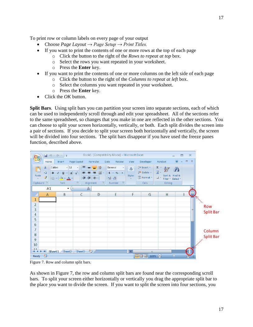
• Click the OK button. Split Bars. Using split bars you can partition your screen into separate sections, each of which can be used to independently scroll through and edit your spreadsheet. All of the sections refer to the same spreadsheet, so changes that you make in one are reflected in the other sections. You can choose to split your screen horizontally, vertically, or both. Each split divides the screen into a pair of sections. If you decide to split your screen both horizontally and vertically, the screen will be divided into four sections. The split bars disappear if you have used the freeze panes function, described above.
RowSplit Bar
ColumnSplit Bar
Figure 7. Row and column split bars. As shown in Figure 7, the row and column split bars are found near the corresponding scroll bars. To split your screen either horizontally or vertically you drag the appropriate split bar to the place you want to divide the screen. If you want to split the screen into four sections, you
18
18
simply use both the row and the column split bars. If you want to remove a split, simply move your cursor over the bar and drag it to the edge of the screen. Hiding and Filtering There are two different functions that allow you to remove either rows or columns from the visible part of the spreadsheet without actually deleting them. The Hide function lets you pick a specific row or column to hide, while the Filter function hides rows that fail to meet a specific criterion you set. Hiding Rows or Columns. Sometimes you want Excel to display, print, or export only a certain subset of the data in your spreadsheet. One way to accomplish this is to hide the rows or columns that you don’t want included. If you want them back at a later point in time, you can then choose to unhide them. You can only hide an entire row or an entire column – you can’t hide a specific selection of cells. To hide a set of rows or columns
• Select the rows or columns you want to hide. • Choose Home → Cells → Format. • Click Hide & Unhide. • Click Hide Columns or Hide Rows depending on what you want to hide.
To unhide a row
• Select both the rows above and below the row you want to unhide. If you want to unhide the first row or first column, you instead move the cursor to the first row and column by entering A1 in the reference box.
• Select the rows or columns you want to unhide. If you wanted to unhide the first row or first column, you don't have to select anything.
• Choose Home → Cells → Format. • Click Hide & Unhide. • Click Unhide Columns or Unhide Rows depending on what you want to unhide.
Filtering Rows. Sometimes you may only want to see cases that have particular values on a variable. In this case you can ask Excel to filter your spreadsheet. There are two ways to establish a filter. Using the autofilter, you can limit the visible rows to those that have a particular value in a column. To turn on the autofilter
• Make sure that your first row contains the names of the variables. The autofilter can only be used if you have such a header row.
• Choose Data → Sort & Filter → Filter. Once you turn on the autofilter, you will see that the first row in every column now has a pull-down menu associated with it. If click on the pull-down menu for a column, you will see a list of all of the values that appear in that column. Next to each value is a checkbox. If the box is checked, rows with that value are displayed. If it is not checked, then rows with that value are hidden. If you select a value, then Excel will only display the rows that have that value. If you
19
19
check the box next to (Select All), then Excel will not filter the rows based on the values in that column (although it may still limit the displayed rows based on the autofilter settings for other columns. The icon of the pull-down button for a given column will change whenever your data set is currently being filtered based on the values in that column (it will look like a funnel with an arrow instead of just an arrow). To turn off the autofilter you simply choose Data → Sort & Filter → Filter a second time. You can also use the advanced filter, which allows you to base the filtering on much more complex conditions. Just like the autofilter, you can only use the advanced filter if you have a header row. To use the advanced filter you must first locate a place at least one cell away from the data for you to type in a filter criteria table. The filter criteria table should be placed either above or below your data table so that the filtering process does not hide it. In the first row of this table, you put the labels for the columns that will be used to form your criteria. The rows below the labels are used to define your criteria. To be visible after filtering, a row in the data set must meet the criteria described in at least one of the filter rows. For a row in the data set to meet the criteria of a filter row, its values must match any limits defined in the columns of the filter row. Therefore, you can make a criterion more restrictive by adding limits in additional columns of the filter row. You can make the filter as a whole less restrictive by adding additional rows to the filter table. This is a bit abstract, so we’ll look at some concrete examples. Imagine that we had a data set containing information about different countries. One column contains the name of the country, one contains the name of the continent the country is on, and one contains the population of the country. If we wanted to only view the entry for Germany, we would use the following filter criteria table. Country Germany If we wanted to see all of the countries that were either in Africa, Europe, or Asia, you would use the following filter criteria table. Continent Africa Europe Asia If we wanted to see all countries in Asia with populations less than 10,000,000, you would use the following filter criteria table. Continent Population Asia <10000000 If you wanted to see countries in Africa, Europe, and Asia that had populations less than 10,000,000, you would use the following filter criteria table.
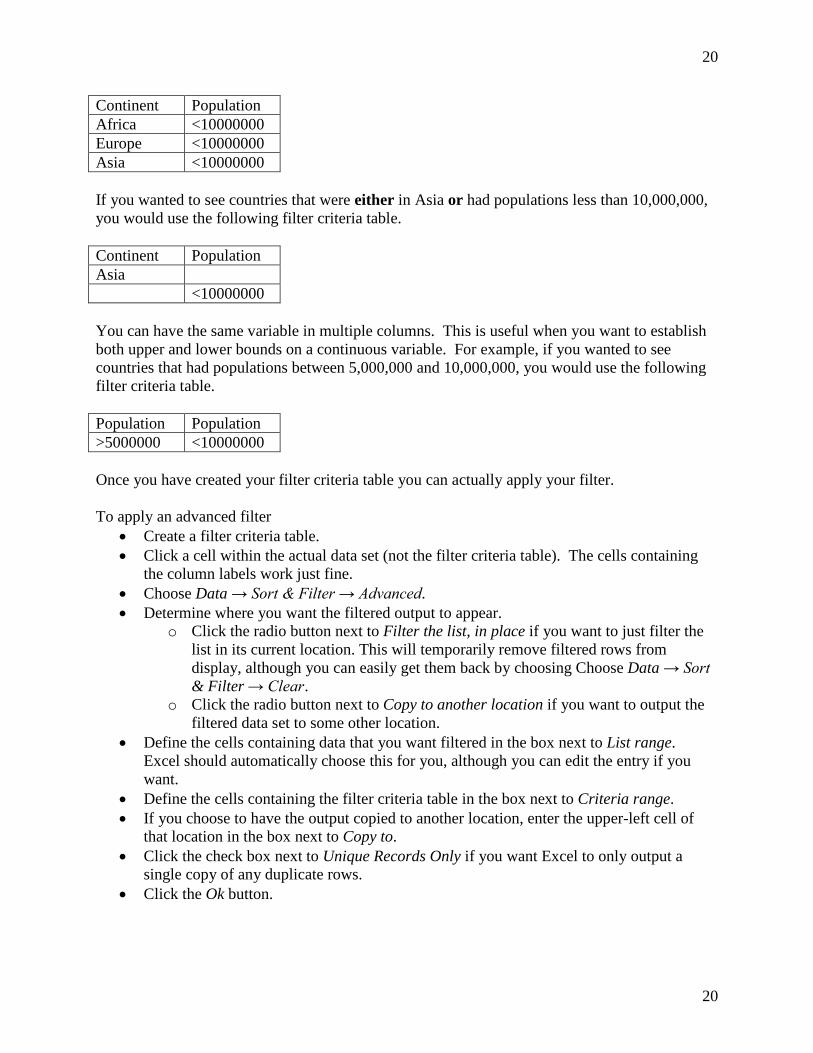
20
20
Continent Population Africa <10000000 Europe <10000000 Asia <10000000 If you wanted to see countries that were either in Asia or had populations less than 10,000,000, you would use the following filter criteria table. Continent Population Asia <10000000 You can have the same variable in multiple columns. This is useful when you want to establish both upper and lower bounds on a continuous variable. For example, if you wanted to see countries that had populations between 5,000,000 and 10,000,000, you would use the following filter criteria table. Population Population >5000000 <10000000 Once you have created your filter criteria table you can actually apply your filter. To apply an advanced filter
• Create a filter criteria table. • Click a cell within the actual data set (not the filter criteria table). The cells containing
the column labels work just fine. • Choose Data → Sort & Filter → Advanced. • Determine where you want the filtered output to appear.
o Click the radio button next to Filter the list, in place if you want to just filter the list in its current location. This will temporarily remove filtered rows from display, although you can easily get them back by choosing Choose Data → Sort & Filter → Clear.
o Click the radio button next to Copy to another location if you want to output the filtered data set to some other location.
• Define the cells containing data that you want filtered in the box next to List range. Excel should automatically choose this for you, although you can edit the entry if you want.
• Define the cells containing the filter criteria table in the box next to Criteria range. • If you choose to have the output copied to another location, enter the upper-left cell of
that location in the box next to Copy to. • Click the check box next to Unique Records Only if you want Excel to only output a
single copy of any duplicate rows. • Click the Ok button.
21
21
Notice that changing the characteristics of your filter table does not immediately affect the content of the data table. If you want to update your filter you must click on a cell within the table and then choose Data → Sort & Filter → Advanced again. To turn off the advanced filter you choose Data → Sort & Filter → Clear. Sorting Data Excel can arrange the values in the rows of your spreadsheet so that they are in either ascending or descending order with regard to the values in a column. You can sort data based on the values of one, two, or three columns. If you want to sort your data based on the value of two or three columns, Excel will sort first on one column, then within the levels of the first column it will sort on the value of the second column, and so forth. Typically you will apply the results of the sort to all of the columns in your spreadsheet in order to maintain the linkages between items in the same row. However, the sort does not have to affect the entire spreadsheet – you can just sort the values in a single column if you want. To sort your data
• Select the section of your spreadsheet you want sorted. If you only select a single cell, Excel will sort the entire spreadsheet.
• Choose Data → Sort & Filter → Sort. • If the first row in your spreadsheet contains the names of the columns, check the box next
to My data has headers. • Select the column you want to base the sort on using the pull-down menu beneath
Column. • Select what you want the values sorted by using the pull-down menu beneath Sort On.
You will usually want this set to Values. • Select the order in which you want the values sorted using the pull-down menu beneath
Order. • If you want to sort on additional columns, click Add Level. This will give you additional
rows on which you can define sorting criteria. Excel will first sort your data by the variable in the first row. If you have multiple rows with the same level on the first variable, it will then sort them within that level based on the sort defined in your second row. You can have as many sort criteria as you like.
22
22
FORMULAS Up to this point we have assumed that the user enters all of the values in the Excel spreadsheet. However, one of the most useful features of Excel is that you can define the value of a cell to be the result of a formula. Using formulas can save you a lot of work compared to doing the calculations by hand. Anything that you would ordinarily do using a calculator can be done in Excel. In addition, you can have the formula make reference to other cells of the spreadsheet, so that the calculated value for one cell depends on the entry found in one or more other cells of the spreadsheet. You can quickly see how changes in that variable affect the results of the formula by simply altering the values in those cells. To have the value of a cell determined by a formula, you type an equals sign (=) as the first character in the cell. You can also just click the equals sign found in the formula bar. You then type out the formula that Excel should use to determine the result of that cell. There are many different things you can have in the formula, such as
• Numbers • Cell references (written in the standard Excel format, such as B10 or E6) • Arithmetic operations
o Addition (+) o Subtraction (-) o Multiplication (*) o Division (/) o Raising something to a power (^)
• Parentheses (used to determine the order in which calculations are made) • Functions (preset computations based either on a single value, such as a cosine, or a
range of values, such as an average) Formulas Without Functions Creating formulas without functions is relatively easy. In this case, you can type out the formulas just like you would type them out on a normal calculator. For example, if you just wanted a cell to be the sum of the values in cells A3 and A4 divided by 10, you would use the formula =(A3+A4)/10 The nice thing about using Excel instead of a calculator is that if you need to do the same basic computation a number of times, you only need to replace the entries in the cells and Excel will automatically calculate the new result. This reduces both the number of keypresses you need to make and your chances of making an error, since you only need to type the formula in once. Excel requires that your formulas follow a specific syntax. For example, you must have an equal number of left and right parentheses in your formula. If for some reason you type in a formula that Excel doesn’t understand, it will give you an error message force you to correct the formula before you can do anything else. If worse comes to worse you can always just delete the entire formula and try again.
23
23
Formulas With Functions Excel has a wide variety of functions that you can use as part of your formulas. A function basically takes an input and provides you with a corresponding output. Sometimes a function requires several different kinds of inputs. Each type of input that a function requires is called an argument. For example, the function FDIST (designed to return the p-value for an F statistic) requires three different arguments: the value of the F statistic, the numerator degrees of freedom, and the denominator degrees of freedom. Each argument may take either a single value, or else it may take multiple values. For example, both the LOG (logarithm) and MIN (minimum) functions have a single argument. However, the argument for the LOG function is a single value, while the argument for the MIN function will typically be a list of values. You must give a function values for all of its arguments for it to give you an output. There are two basic ways to enter a function into a spreadsheet formula. One way to include a function in your formula is to select the formula from the pull-down menu in far left of the formula bar. The menu doesn’t appear until you either click the equals sign in the formula bar or type an equals sign as the first character in a cell. The first pull-down menu contains the most commonly used functions, such as IF, AVERAGE, and STDEV. The last selection in this menu is More Functions, which will allow you to select from a much larger list of functions that is organized in submenus. Clicking on a function in this menu once will provide you with information about that function, including both a list of the arguments it takes as well as a description of what it produces as an output. To select a function, you double-click it. Excel will then open up a window that will help you insert the function into your formula. The window will have a box for each argument the function can take. You can either type arguments directly into each argument box, or else you can click the button at the right-hand side of the box to use the mouse to select cells from the spreadsheet to fill the argument. When you have filled in all the values you click Ok. You do not have to use a mouse if you want to use cells for function arguments. You can also type in cell references manually, using the following guidelines.
• If you want an argument to be equal to the value of a single cell, you simply use the cell reference. For example, B4 (cell B4).
• If you want an argument to be a set of rows or columns, you use the notation start heading:end heading. For example, 12:15 (row 12 through row 15). The values for start heading and end heading would be the same if you only want to include the values in a single row or column. For example, D:D (row D).
• If you want the input for a function to be a set of cells that are in a block somewhere in your spreadsheet you use the notation upper-left cell:lower-right cell. For example, C3:E6 (the 12 cells in the block between C3 and E6).
• If you want an argument to be equal to a set of cells that are not in a block, you can type in their references separated by commas. For example, A1,B2,C3,D4 (cells A1, B2, C3, and D4).
• You can also include multiple rows, columns, and blocks of cells separated by commas if you like. For example, 5:5,D:D,A3 (the cells that are either in row 5, column D, or in cell A3).
24
24
The second way to use a function is to just type it in as part of your formula. When typing in a function you first put the function name, then a left parenthesis, then the function arguments separated by commas, and finally end with a right parenthesis. All of the following would be examples of formulas that include functions.
• =SQRT(2) o Provides the square root of 2
• =LOG(A2) – LOG(B2) o Provides the difference between the logarithm of the value in cell A2 and the
logarithm of the value in cell B2. • =AVERAGE(A2, A3, B3:F22)
o Provides the average of the values in cells A2, A3, and in the box between cells B3 and F22.
• =ZTEST(A:A, 0, 2.5) o Provides the p-value for a Z test comparing the mean of the values in cell A to the
value of 0, assuming that the population standard deviation is 2.5. For functions with multiple arguments like the last example, you cannot use commas to indicate that several cells are part of the same argument because commas are already being used to separate the arguments. For these functions, any arguments based on cells in the spreadsheet must therefore all come from a block that can be identified without using commas. You can use the Excel Help if you want more detailed information about a given function. To activate Excel Help you can either press F1 or else you can click the office assistant. Then you just type in the name of the function that you want to learn more about in the box that appears. Excel should then pop up a list of selections, one of which should offer you help on the specific function you entered. Descriptions of Specific Functions Excel has hundreds of different functions that you can use in your formulas. In this section we will list those that would most likely be of interest to a researcher. Computational Functions. There are functions that can provide you with summary information on a set of cells, such as
• SUM (adds together the cell values) • AVERAGE (arithmetic mean) • STDEV (standard deviation) • VAR (variance) • DEVSQ (sum of squared deviations from the arithmetic mean) • GEOMEAN (geometric mean) • HARMEAN (harmonic mean)
25
25
Order Functions. There are functions that allow you to locate specific observations within a set of cells, such as
• MEDIAN (the value at the 50th percentile) • PERCENTILE (allows you to find a value in the list at the percentile you define) • QUARTILE (allows you to find any of the quartiles) • MIN (minimum value) • MAX (maximum value) • MODE (the most common value) • LARGE (finds the Nth largest item in the list) • SMALL (finds the Nth smallest item in the list)
Transformation Functions. There are also several transformation functions that statisticians might find useful, such as
• LN (natural log) • EXP (exponential function: ex) • SQRT (square root) • STANDARDIZE (outputs the standardized value, where you provide the mean and
standard deviation as arguments) • FISHER (Fisher’s r-to-Z transformation) • FISHERINV (Fisher’s Z-to-r transformation)
Inferential Functions. There are functions that will provide you with an estimate of the relationship between the values in two sets of cells. Most of these functions require two sets of cells as arguments, where the number of cells in each argument is the same. For those functions, corresponding cells in the two arguments would represent measurements on the same object. More advanced statistics can be obtained using Excel’s Analysis Toolpak (described below), but some that can be obtained simply through functions are
• CHITEST (chi-square interaction test for detecting a relationship in a frequencies table) • CORREL (correlation) • COVAR (covariance) • FTEST (Tests whether two variances are equal. Notice that this can only be used to
perform an ANOVA indirectly, requiring you to obtain estimates of the overall and pooled variances on your own.)
• TTEST (t test) • INTERCEPT (provides the intercept from the least-squares regression equation
predicting the second set of cells from the first) • SLOPE (provides the slope from the least-squares regression equation predicting the
second set of cells from the first) • RSQ (r2, indicating the proportion of variance in the second set of cells that can be
explained by the first set of cells)
26
26
Distribution Functions. There are functions that can provide you with the p-values associated with various statistical distributions. Excel also has inverse functions for many of these, which can provide you with the test statistic if you provide the p-value.
• BETADIST, BETAINV (beta distribution) • BINOMDIST (binomial distribution) • CHIDIST, CHIINV (chi-square distribution) • EXPONDIST (exponential distribution) • FDIST, FINV (F distribution) • GAMMADIST, GAMMAINV (gamma distribution) • HYPGEOMDIST (hypergeometric distribution) • LOGNORMDIST, LOGINV (lognormal distribution) • NEGBINOMDIST (negative binomial distribution) • NORMDIST, NORMINV (normal distribution, where you get to provide the mean and
the standard deviation) • NORMSDIST, NORMSINV (standard normal distribution, with a mean of 0 and a
standard deviation of 1) • POISSON (Poisson distribution) • TDIST, TINV (t distribution)
The IF Function. The IF function is one of the most useful functions, earning a discussion in its own section. IF requires three arguments: a condition to be evaluated, a value that the cell would have if the condition is true, and a value that the cell would have if the condition is false. For example, the formula =IF(A2>5, 1, 0) would set the value of this cell to 1 if cell A2 was greater than 5, and would set it to 0 if it was not. You can also have the values set to be text, but you need to enclose the text with quotes. For example, the formula =IF(A2<60, “fail”, “pass”) would set the value of the cell to fail if cell A2 was greater than 60 and pass if it was not. Nested Functions You can actually use the result of one function as the argument for another function. For example, let us say that you had a list of numbers in cells A2 through A21 that you wanted to standardize. The following formula would standardize the first value, and similar formulas could be used to standardize the remaining formulas. =STANDARDIZE(A2, AVERAGE(A2:A21), STDEV(A2:A21)) The STANDARDIZE function takes three arguments: a value to standardize, as well as the mean and standard deviation of the distribution on which you want to base the standardization. Instead
27
27
of having constant values for the mean and standard deviation, the formula above computes these as the average and standard deviation of the values in cells A2 through A21. As a second example, let us say that you wanted to test whether mean of the values in these cells is significantly different from another variable measured on the same subjects, contained in cells B2 through B21. To do this you must first calculate a t-statistic, and then determine whether the p-value for this statistic is less than.05. Normally we would have to do this as two separate steps, computing the test statistic with the formula =TTEST(A2:A21, B2:B21, 1) And then taking the result of that (which we’ll call T) and putting it into the formula =TDIST(T, 18, 1) However, the following nested formula does it in a single step. =TDIST(TTEST(A2:A21, B2:B21, 1), 18, 1) Nested IF Functions. One of the most useful ways to use nesting is with the IF function, where you put an IF function as one of the last two arguments of another IF function. The formula below is an example of a nested IF function. =IF(A2<60, “low”, IF (A2<80, “medium”, “high”)) This formula actually can result in three different values. If the value of cell A2 is below 60 then the formula produces the result low. If the value of A2 is 60 or above then Excel moves to the second IF function. In this case, the formula produces the result medium if the value of cell A2 is below 80, and produces the result high if it is not. The end result is that this formula can produce three different values: low if cell A2 is below 60, medium if cell A2 is 60 or above but less than 80, and high if cell A2 is 80 or above. Even though their conditions overlap, there is no confusion between the low and medium categories because the second IF function will never be evaluated if the value of A2 is below 60. It is possible to extend the idea of nested IF functions even further, providing you with an easy way to create a set of categories based on the value of a continuous variable. For example, let us say that the value in cell A2 represented a percentile score, on which we wanted to base a set of grades. This could be done using the formula =IF(a2<60, “F”, IF(a2<70, “D”, IF(a2<80, “C”, IF(a2<90, “B”, “A”)))) This formula produces the value F if cell A2 is below 60, the value D if cell A2 is 60 or above but below 70, the value C if cell A2 is 70 or above but below 80, the value B if cell A2 is 80 or above but below 90, and the value A if cell A2 is 90 or above.
28
28
As you can see, you can use nested IF formulas to create a set of categorical values based on a continuous value found in another cell. You will end up needing a number of IFs equal to the number of categories you want – 1. However, Excel will only allow you to nest a total of 8 functions, for a maximum of 9 different categories. Luckily, there is a way to get around this limit by spreading your formula across different columns. Let us say that the value in cell A2 represented a percentile score, and you wanted to use a formula to assign a grade using the +/- system (A, A-, B+, B, B-, C+, C, C-, D, F). Here we have 10 categories, so we can’t use a single formula to assign the grade. What we will do instead is use one column (B2) to assign the grade if it is a C, D, or F, a second column (C2) to assign the grade if it is an A or B, and then a third column (D2) to combine the results from the first two so that we can have all the grades in a single column. The formula in cell B2 would be =IF(A2<60, "F", IF( A2<70, "D", IF(A2<73, "C-", IF(A2<77, "C", IF(A2<80, "C+", -1))))) the formula in cell C2 would be =IF(A2<80, -1, IF(A2<83, "B-", IF(A2<87, "B", IF(A2<90, "B+", IF(A2<93, "A-", "A"))))) and the formula in cell D2 would be =IF(B2=-1, C2, B2) If the grade is between an F and C+, it appears in cell B2 and a –1 appears in cell C2. If the grade is between B- and A, it appears in cell C2 and a –1 appears in cell B2. Cell D2 takes on the value of whichever of those two columns does not have a value of –1. You can therefore always find the grade in column D2, no matter what it is. Copy and Paste with Formulas After copying a cell containing a formula, you have two different ways to paste it into a new cell. You can either paste the formula that was used to generate the cell value, or you can paste the cell value itself (separating it from the formula). Copying the Formula. You can simply use the standard copy and paste commands listed above if you want to copy the formula from the cell. Excel will automatically update any cell references so that the new formula refers to cells in the same relative location as in the original formula. For example, if you copy the formula =SQRT(A2) from cell B2 and then copy it into cell B3, Excel would automatically update it to be =SQRT(A3)
29
29
since cell A3 is in the same location relative to cell B3 (one to the left) as cell A2 was to the original cell B2. If you don’t want Excel to change a particular cell reference in a formula, you should put a dollar sign ($) in front of the column letter and the row number. So, if you wanted to copy the above formula in cell B2 but always wanted the formula to refer to cell A2 when it was copied, the formula should be =SQRT($A$2) You can also allow Excel to update only the row or only the column reference. In this case you would put a dollar sign in front of whichever part you didn’t want to change. For example, let us say that you always wanted the formula to refer to the cell that is in the same row as where you copy it, but always wanted it to refer to the value in column A, no matter what column you end up copying it to. In this case, the formula should be =SQRT($A2) Copying the Value. Sometimes you just want to copy the value in the cell and not the formula. To do this you would
• Select the cells to be copied. • Select the copy function. • Select the cell you want to copy the value into. • Choose Home → Clipboard → Paste More. • Click Paste Special. • Click the button next to Values. • Click the Ok button.
In this case, the new cells would contain the values from the copied columns. However, these are no longer being calculated by a formula, and so would not automatically update if you changed other parts of the spreadsheet. Goal Seek Goal seek allows you to work with your formula in the reverse direction. It requires that you have a formula that results in a numeric value as a function of the values in other cells of the spreadsheet. You can then specify a value that you want the formula to have, and Excel will figure out what input value you will need to get it. Goal seek only works with one input at a time. If your formula references more than one other cell, you will need to choose one to be the target of the procedure. To use goal seek
• Choose Data → Data Tools → What-if Analysis. • Click Goal Seek. • Type the name of the cell whose formula you want to use in the box beside Set cell. • Type the formula result that you want in the box beside To value.

30
30
• Type the name of the input cell whose value you want to change in order to get the new formula value in the box beside By changing cell.
• Click Ok.
31
31
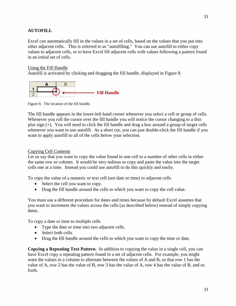
AUTOFILL Excel can automatically fill in the values in a set of cells, based on the values that you put into other adjacent cells. This is referred to as “autofilling.” You can use autofill to either copy values to adjacent cells, or to have Excel fill adjacent cells with values following a pattern found in an initial set of cells. Using the Fill Handle Autofill is activated by clicking and dragging the fill handle, displayed in Figure 8. Figure 8. The location of the fill handle. The fill handle appears in the lower-left hand corner whenever you select a cell or group of cells. Whenever you roll the cursor over the fill handle you will notice the cursor changing to a thin plus sign (+). You will need to click the fill handle and drag a box around a group of target cells whenever you want to use autofill. As a short cut, you can just double-click the fill handle if you want to apply autofill to all of the cells below your selection. Copying Cell Contents Let us say that you want to copy the value found in one cell to a number of other cells in either the same row or column. It would be very tedious to copy and paste the value into the target cells one at a time. Instead you could use autofill to do this quickly and easily. To copy the value of a numeric or text cell (not date or time) to adjacent cells
• Select the cell you want to copy. • Drag the fill handle around the cells to which you want to copy the cell value.
You must use a different procedure for dates and times because by default Excel assumes that you want to increment the values across the cells (as described below) instead of simply copying them. To copy a date or time to multiple cells
• Type the date or time into two adjacent cells. • Select both cells. • Drag the fill handle around the cells to which you want to copy the time or date.
Copying a Repeating Text Pattern. In addition to copying the value in a single cell, you can have Excel copy a repeating pattern found in a set of adjacent cells. For example, you might want the values in a column to alternate between the values of A and B, so that row 1 has the value of A, row 2 has the value of B, row 3 has the value of A, row 4 has the value of B, and so forth.
Fill Handle
32
32
To copy a repeating pattern of text
• Select a set of adjacent cells defining the pattern. • Drag the fill handle around the cells to which you want to copy the pattern. You may end
up with incomplete copies of the pattern if you select a number of cells that is not evenly divided by the number of cells in the pattern.
To have Excel repeat a pattern of numbers
• Select the column in which you want the pattern to repeat. • Set the content type to Text using the pulldown menu in the Home → Number command
group. • Type the sequence you want to repeat, with one number in each cell, at the top of the
column. • Select the cells composing the sequence. • Drag the fill around the cells in which you want the sequence to repeat.
Incrementing Cell Values Autofill can also be used to have Excel generate a list of incremented values. For example, let us say that you wanted the different rows to represent different days of the year, and that you wanted the value in the first column to be the date. It would be very tedious to fill in the values of this column by hand. Using autofill, you can type in the first date and then use the autofill function to automatically generate the appropriate values for the remaining 364 rows. To generate a list of automatically incremented dates or times
• Select the cell containing the date or time • Drag the fill handle around the cells to which you want to copy the cell value.
o If you drag the cursor up or to the left, then the next cells will have increasingly earlier dates or times.
o If you drag the cursor down or to the right, then the next cells will have increasingly later dates or times.
By default, Excel will increment days by 1 day and times by 1 hour. If you want to create a list using a different increment
• Type the first two dates or times in the list in two adjacent cells. • Select both cells. • Drag the fill handle around the cells to which you want to copy the cell value.
o If you drag the cursor up or to the left, then the cells will be decreased by the increment that you define.
o If you drag the cursor down or to the right, then the cells will be increased by the increment that you define.
To generate a list of incremented numbers (which can be incremented by any constant amount)
• Type the first two numbers in the list in two adjacent cells. • Select both cells.
33
33
o Drag the fill handle around the cells to which you want to copy the cell value. If you drag the cursor up or to the left, then the next cells will have numbers decreased by the increment you define.
o If you drag the cursor down or to the right, then the next cells will have numbers increased by the increment you define.
Formulas To use autofill to copy a formula from one cell to adjacent cells
• Select the cell containing the formula you want to copy. • Drag the fill handle around the cells to which you want to copy the cell value.
When you copy formulas using autofill, Excel will automatically change the cell references in the formula so that they refer to cells in the same relative location as those in the original formula. For example, let us say you have a formula in cell A6 that calculates the sum of the values in cells A1 through A5. If you autofill to copy the formula to cell B6, the new formula will calculate the sum of the values in cells B1 through B5. You can prevent Excel from making these changes by putting a dollar sign ($) in front of any elements that you want to stay constant. More detail on this can be found in the section on Copy and Paste with Formulas. People will often write formulas that calculate something based on the values within the same row. Using autofill you can easily apply such a formula to all of the rows in your spreadsheet. The easiest way to do this is to first define the formula in the top row of the data set and then use autofill to copy the formula to all the below it in the same column.
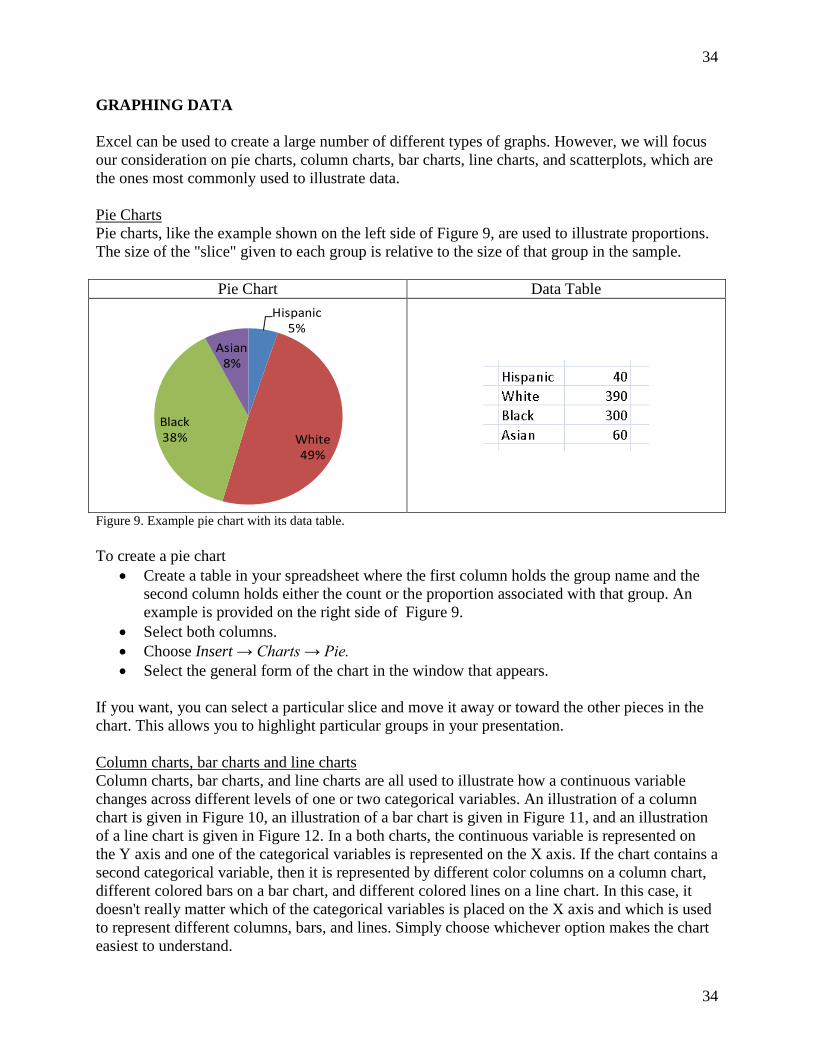
34
34
GRAPHING DATA Excel can be used to create a large number of different types of graphs. However, we will focus our consideration on pie charts, column charts, bar charts, line charts, and scatterplots, which are the ones most commonly used to illustrate data. Pie Charts Pie charts, like the example shown on the left side of Figure 9, are used to illustrate proportions. The size of the "slice" given to each group is relative to the size of that group in the sample.
Pie Chart Data Table Hispanic
5%
White49%
Black38%
Asian8%
Figure 9. Example pie chart with its data table. To create a pie chart
• Create a table in your spreadsheet where the first column holds the group name and the second column holds either the count or the proportion associated with that group. An example is provided on the right side of Figure 9.
• Select both columns. • Choose Insert → Charts → Pie. • Select the general form of the chart in the window that appears.
If you want, you can select a particular slice and move it away or toward the other pieces in the chart. This allows you to highlight particular groups in your presentation. Column charts, bar charts and line charts Column charts, bar charts, and line charts are all used to illustrate how a continuous variable changes across different levels of one or two categorical variables. An illustration of a column chart is given in Figure 10, an illustration of a bar chart is given in Figure 11, and an illustration of a line chart is given in Figure 12. In a both charts, the continuous variable is represented on the Y axis and one of the categorical variables is represented on the X axis. If the chart contains a second categorical variable, then it is represented by different color columns on a column chart, different colored bars on a bar chart, and different colored lines on a line chart. In this case, it doesn't really matter which of the categorical variables is placed on the X axis and which is used to represent different columns, bars, and lines. Simply choose whichever option makes the chart easiest to understand.
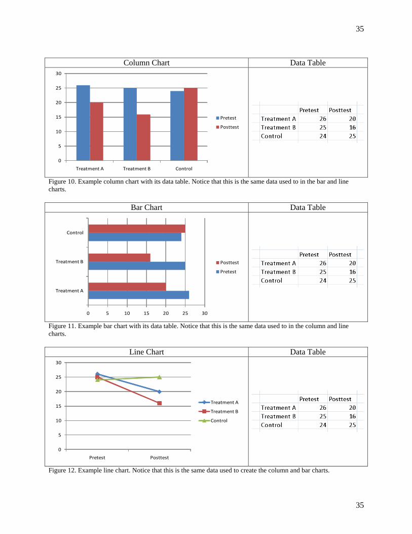
35
35
Column Chart Data Table
0
5
10
15
20
25
30
Treatment A Treatment B Control
Pretest
Posttest
Figure 10. Example column chart with its data table. Notice that this is the same data used to in the bar and line charts.
Bar Chart Data Table
0 5 10 15 20 25 30
Treatment A
Treatment B
Control
Posttest
Pretest
Figure 11. Example bar chart with its data table. Notice that this is the same data used to in the column and line charts.
Line Chart Data Table
0
5
10
15
20
25
30
Pretest Posttest
Treatment A
Treatment B
Control
Figure 12. Example line chart. Notice that this is the same data used to create the column and bar charts.
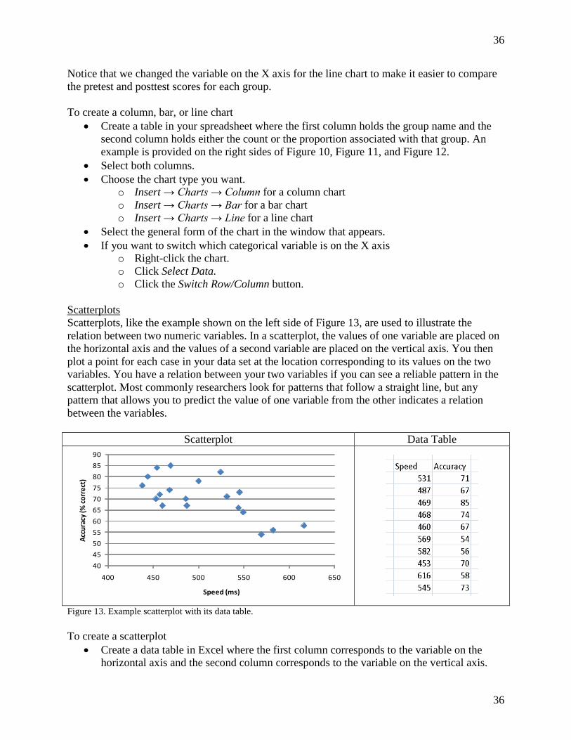
36
36
Notice that we changed the variable on the X axis for the line chart to make it easier to compare the pretest and posttest scores for each group. To create a column, bar, or line chart
• Create a table in your spreadsheet where the first column holds the group name and the second column holds either the count or the proportion associated with that group. An example is provided on the right sides of Figure 10, Figure 11, and Figure 12.
• Select both columns. • Choose the chart type you want.
o Insert → Charts → Column for a column chart o Insert → Charts → Bar for a bar chart o Insert → Charts → Line for a line chart
• Select the general form of the chart in the window that appears. • If you want to switch which categorical variable is on the X axis
o Right-click the chart. o Click Select Data. o Click the Switch Row/Column button.
Scatterplots Scatterplots, like the example shown on the left side of Figure 13, are used to illustrate the relation between two numeric variables. In a scatterplot, the values of one variable are placed on the horizontal axis and the values of a second variable are placed on the vertical axis. You then plot a point for each case in your data set at the location corresponding to its values on the two variables. You have a relation between your two variables if you can see a reliable pattern in the scatterplot. Most commonly researchers look for patterns that follow a straight line, but any pattern that allows you to predict the value of one variable from the other indicates a relation between the variables.
Scatterplot Data Table
4045505560657075808590
400 450 500 550 600 650
Accu
racy
(% co
rrec
t)
Speed (ms)
Figure 13. Example scatterplot with its data table. To create a scatterplot
• Create a data table in Excel where the first column corresponds to the variable on the horizontal axis and the second column corresponds to the variable on the vertical axis.
37
37
You should have one line in the table for each point on the plot. An example is provided on the right side of Figure 13.
• Select both columns. • Choose Insert → Charts → Scatter. • Select the general form of the chart in the window that appears.
Customizing Charts Each of the different types of charts can be highly customized. You can customize the overall chart appearance, you can select the colors, fill, and line styles of different chart elements, and select the content, font, and style of the row and column titles. Clicking on a chart will add three "Chart Tools" to your tabs: Design, Layout, and Format. Below are the most useful functions for customizing the appearance of the chart.
• The Design → Chart Layout command group offers you a number of variations on how the chart is set up and how the elements of the chart are labeled. For example, when a pie chart is selected, the this command group will allow you to choose from a chart that includes the percentages and group names in the chart, one which has the percentages in the chart and the group names in a legend, and one which only has the group names in the chart.
• The Design → Chart Styles command group offers you a number of different color schemes for your chart.
• The Layout → Insert command group provides commands that allow you to add new elements to the chart, like text boxes and shapes.
• The Layout → Labels command group provides commands that let you put labels on the top of the chart or on the chart axes. You can control the font, font size, effects, and orientation of the labels.
• The Format → Size command group allows you to change the dimensions of the chart. By default, changing one dimension will automatically resize the other dimension to keep the same aspect ratio.
If you right-click a pie slice, column, bar, line, or point and then select Format Data Series, Excel will allow you to change the color or pattern associated with that group throughout the chart. The exact options that are available will depend on the type of chart, but in any case, the choices you make here will only apply to the selected group. If you right-click an axis in your graph and then select Format Axis you can customize the range of values that are displayed on the axis.
38
38
IMPORTING AND EXPORTING FILES While it is quite possible to work a data set of data entirely within Excel, often times you may want to combine your work in Excel with some other program. For example, you may come across a data set that was originally entered in Word that you want to examine within Excel. Alternatively, you might want to export a data set created in to a more powerful program for data analysis, such as SPSS or SAS. Luckily, Excel has functions that make it easy to both import and export data. Importing Data from a Word Processor Formatting the Word Processing Document. In order for you to read in data from a word processor you must have the document organized in a way that allows Excel to know what values should be placed in what columns in the spreadsheet. There are two different ways to do this. In a delimited file, data that will go into different columns in the spreadsheet are separated by a specific character, such as a tab, space, or comma. A delimited file (using a comma as the delimiter) would look something like 1,1,tudor mansion,434 1,2,car,446 1,3,koala bear,331 2,1,swiss chalet,843 2,2,boat,754 2,3,tiger,1023 You must be careful to choose an appropriate delimiter. Specifically, your delimiter should not be a character that would actually appear in any of the entries, or else Excel will not be able to tell when the character should be considered part of a cell value and when the character should be treated as a delimiter. For example, it would be inappropriate to use a space as a delimiter in the data set above because some of the actual data entries contain spaces. Usually the tab character is a good choice for a delimiter. In a fixed-width file, data that will go into different columns in the spreadsheet are placed in specific columns in text file. A fixed-width file would look something like 11tudormansion 434 12car 446 13koala bear 331 21swiss chalet 843 22boat 754 23tiger 1023 Here, for example, the content of the third spreadsheet column would always be contained in columns 3 through 17 in the word document. You should be careful when entering in data in a fixed-width format, because many fonts don’t make all of the letters the same width. In this case you could have two words that appear to be in the same location but which are actually in different columns. It is therefore always a good idea to use nonproportional font (such as courier) when working with a fixed-width file in a word processor.
39
39
Excel can read both delimited and fixed-width files. Each provides you with a clear way of knowing what characters from the text file should be placed into each column in the spreadsheet. However, most people find delimited files easier to work with than fixed-width files. Once you have a word-processing document that is in either a delimited or fixed-width format, you save it as a “text file” before you can try to load it into Excel. A text file contains all the words and numbers from the document, but does not have any special formatting. Any word processor will allow you to save a file in text format. To save a Word document as a text file
• Choose Windows button → Save as. • Click the button on the right-hand side of the Save as type box. • Choose Text Only. • Click the Save button.
Reading a Text File Into Excel. Once you have saved the data as a text file, you must now load it into Excel. To read a text file into Excel
• Choose Windows button → Open. • Click the button on the right-hand side of the Files of type box. • Choose Text Files. • Either select the file you want to open using the explorer window or type the name
directly into the File name box. • Click the Open button. • Click the radio button next to either Delimited or Fixed Width to indicate the way that
you formatted the text file. • Click the Next button. • For delimited data files
o At the top of the next window, Excel will ask you to indicate what characters you used as delimiters. Make sure that the boxes next to your delimiters are checked and those that are not your delimiters are unchecked.
o Excel will now show you how it thinks you want to divide the contents of the file into different spreadsheet cells. This should be correct if you applied the formatting properly.
o Click the Next button. • For fixed-width data files
o Excel will now show you how it thinks you want to divide the contents of the file into different spreadsheet cells. Excel does its best to guess where the divisions should be, but you may need to make changes to import the file properly. You can move existing divisions by clicking on the dividing line and dragging it to a new location. You can completely remove a divider by dragging its line outside the box. You can add a new division by clicking on a location where there currently is no line.
o Click the Next button. • Excel now provides you with the opportunity to define the variable type for each
spreadsheet column. By default, Excel assumes that each column will be of the General
40
40
type, which automatically converts cells with numbers to numeric format and cells with letters to text format. There is usually no need to change this.
• Click the Finish button. At this point the data from your word processing document should be imported into an Excel spreadsheet. Importing Data from SPSS or SAS To convert an SPSS data set to an Excel file
• Open the data set you want to convert • Choose File → Save as • Click the button on the right-hand side of the Save as type box. • Choose Excel. • Click the Save button.
You can use the following code to convert a SAS data set to an Excel file. PROC DBLOAD DBMS=xls DATA=sasdata; PATH='c:\exceldata.xls'; PUTNAMES=yes; LOAD; RUN; You should replace sasdata in the first line with the name of the SAS data set you want to convert, and you should replace c:\exceldata.xls in the second line with the path and filename of the Excel file that you want SAS to create. Exporting Data to a Word Processor You can use the basic copy and paste functions to copy the contents of an Excel spreadsheet into a word processing program. In this case, the contents of the spreadsheet will usually appear as a table in the word processing document. You also have the option of saving the contents of a spreadsheet to a text file, if you want to load it into a word processor just as a set of characters on a line instead of entries in a table. To save an Excel spreadsheet as a text file
• Choose Windows button → Save as. • Click the button on the right-hand side of the Save as type box. • Choose Text (tab delimited). • Click the Save button.
Excel will then convert the contents of your spreadsheet to a tab-delimited text file, which should be readable by any word processor. Exporting Data to SPSS or SAS Both SAS and SPSS can directly load Excel files as data sets. You don't need to format them in any special way. However, you should try to make your column names match the variable name
41
41
requirements of whichever software you will be using or else your variables will be renamed by the statistical software. To load an Excel worksheet into SPSS
• Choose File → Open → Data • Click the button on the right-hand side of the Files of type box • Choose Excel. • Either select the file you want to open using the explorer window or type the name
directly into the File name box. • Click the Open button. • Click the check box next to Read variable names if the first row of your spreadsheet
contains the variable names. • Click the Ok button.
To load an Excel worksheet into SAS
• Choose File → Import Data • Check the box next to Standard Data Source • Choose Microsoft Excel Spreadsheet from the drop-down menu. • Click the Next button. • Enter the path and filename of the Excel spreadsheet in the box that appears. You can
also click the Browse button to find the file using Windows Explorer. • Click the Next button. • Type in the name you want to give the data set in the box beneath Member. • Click the Finish button.
This also provides an easy way to transport data sets between SAS and SPSS. You go to the original program and convert the data set to Excel format (as described in Importing Data from SPSS or SAS). You then go to the second program and import the Excel data set you just created.
42
42
THE ANALYSIS TOOLPAK Although it is not well known, Excel has the ability to perform a wide variety of statistical analyses. These are performed using the Analysis Toolpak, which is a statistical add-in that is distributed with Excel. The Toolpak will allow you to calculate descriptive statistics, t-tests, correlations, regressions, and ANOVAs. The Toolpak also contains procedures that allow you to generate lists of random numbers. Installation While the Analysis Toolpak is distributed with Excel, it is typically not installed automatically. To see if it is installed you should open up the Tools menu. If there is a Data Analysis selection available, then the Toolpak is already installed. If the selection is not available, then the Toolpak is not installed. To install the Analysis Toolpak
• Choose Microsoft button → Excel Options. This button is on the bottom of the window, rather than on the left.
• Click Add-ins. • Click Analysis Toolpak. • Click the Go button next to the Manage pulldown at the bottom of the screen. • A window will pop up with a list of addons. Check the box next to Analysis Toolpak. • Click Ok. • Excel will then take you through a set of installation screens. You should follow the
instructions it gives you. o The file required to install the Toolpak, Analys32.xll, may or may not have been
copied to your computer when you originally installed Excel. If it was, it should be located in C:\Program Files\Microsoft Office\Office\Library\Analysis If it is there, Excel should detect the file automatically.
o If the file was not originally copied to your computer, you will need to insert your Microsoft Office disk in order to complete the installation.
Once the installation is finished, you should have an Analysis command group added to the Data tab in Excel. Analysis Input and Output In a data set, different columns typically represent different variables, while different rows represent different subjects. The value in a particular cell within the table would therefore be the value on the variable corresponding to its column for the subject corresponding to its row. However, Excel does give you the option of reversing the organization of the data, so that the rows correspond to variables and the columns correspond to subjects. Each of these functions will produce a reasonably detailed output. This output will take up several rows and columns, so you will need to specify where you want it to be placed for each of these procedures. There are three options.
43
43
• You can put the results in the current spreadsheet. If you want to use this option, you will need to specify the cell which will be the upper-left hand corner the output.
• You can put the results in a new spreadsheet in the current file. • You can put the results in a new file.
The output will often contain values that will exceed the standard cell widths, so you will probably want to resize the columns containing the output. The easiest way to do this would be to select the output columns and then autofit the column width. Descriptive Statistics Descriptive statistics provide you with information about the distribution of a single variable. To receive descriptive statistics on a set of cells
• Choose Data → Analysis → Data Analysis. • Select Descriptive Statistics. • Click the Ok button. • Define the range of cells you want to examine in the Input Range box. You can select
entire rows or columns if you like. • Indicate whether the variables in your data set correspond to rows or columns by clicking
the appropriate radio button next to Grouped By. Excel will provide separate statistics for each variable.
• If the first row or column in your selection contains labels, click the box next to Labels in First Row/Column.
• Choose where you want the results to be printed using the radio buttons at the top of the Output Options box.
• Click the box next to whichever statistics you want to see. o Summary Statistics provides all the basic descriptive statistics, including the
mean, median, mode, standard deviation, and sum. o Confidence Interval for Mean will, not surprisingly, provide you with a
confidence interval around the mean. You can specify what confidence level you want to use.
o Kth Largest sorts your data and finds the cell that is K down from the top. o Kth Smallest sorts your data and finds the cell that is K up from the bottom.
You may want to autofit the columns containing the output so that you can read it easier. Inferential Statistics Inferential statistics allow you to determine the relationship between two or more variables measured on a group of subjects. Correlation. A correlation provides a measure of the linear relationship between a pair of numeric variables. If your variables contained in different columns, then Excel assumes that values from the same row are taken from the same subject. If your variables are contained in different rows, then Excel assumes that values in the same column are taken from the same subject. A table that displays all of the correlations among a set of variables is called a correlation matrix.
44
44
To obtain a correlation matrix for a group of variables
• Choose Data → Analysis → Data Analysis. • Select Correlation. • Click the Ok button. • Define the range of cells you want to examine in the Input Range box. You can select
entire rows or columns if you like. • Indicate whether the variables in your data set correspond to rows or columns by clicking
the appropriate radio button next to Grouped By. • If the first row or column in your selection contains labels, click the box next to Labels in
First Row/Column. • Choose where you want the results to be printed using the radio buttons in the Output
Options box. • Click the Ok button.
The output for a correlation analysis contains a table with the names of the variables listed both on the top row and on the left column. The value in the table will be the correlation between the variable listed at the top of its column and the variable listed to the left of its row. Linear Regression. Linear regression allows you to build an equation that predicts the value of a dependent variable (DV) from the value of one or more independent variables (IVs). It also allows you to determine whether each IV can account for a significant amount of the variability in the DV. Unlike correlations, for linear regression your data must be organized so that the variables correspond to the columns and the subjects correspond to the rows. To conduct a simple linear regression
• Choose Data → Analysis → Data Analysis. • Select Regression • Click the Ok button. • Define the range of cells composing the DV in the Input Y Range box. You must provide
the specific cell references for the DV – you cannot simply specify an entire column. • Define the range of cells that compose the IVs in the Input X Range box. Each column
that you specify will represent a different IV. The IVs must be next to each other, and each have the same number of cells as the DV. Just like with the DV, you need to provide the specific cell references that define the set of IVs.
• If the first row contains the variable names, check the box next to Labels. • If you want to build a regression model that does not have an intercept parameter, check
the box next to Constant is Zero. • By default Excel will produce 95% confidence intervals around the regression model
parameters. If you want a set of confidence intervals using a different confidence level o Check the box to the left of Confidence Level. o Enter the confidence level you want in the box to the left of the percent sign.
• Choose where you want the results to be printed using the radio buttons at the top of the Output Options box.
45
45
• You can have Excel provide a number of diagnostics for the regression model in the output.
o Checking the box next to Residuals will provide you with a list of the unstandardized residuals.
o Checking the box next to Standardized Residuals will provide you with a list of the standardized residuals
o Checking the box next to Residual Plots will provide you with a set of graphs, each plotting the values of an IV versus the residuals.
o Checking the box next to Line Fit Plots will provide you with a graph of the predicted values versus the observed values.
o Checking the box next to Normal Probability Plot will provide you with a graph of the percentiles of your residuals compared to the percentiles of the standard normal distribution. If your residuals are normally distributed you would expect this plot to be approximately a straight line.
• Click the Ok button. The output for a regression analysis will include model characteristics, such as the R2 and adjusted R2, an ANOVA table for the full model, the model parameters, and a statistical test of the significance of each parameter. While Excel does not provide you with an option to create interaction terms between the components in your model, you can always create them yourself manually by adding a new column to your data set that is the product of the two variables whose interaction you want to examine. Within-Subjects t-Test. A within-subjects t-test is used to test for a difference between the means of two variables measured on the same subjects. If your variables contained in different columns, then Excel assumes that values from the same row are taken from the same subject. If your variables are contained in different rows, then Excel assumes that values in the same column are taken from the same subject. To perform a within-subjects t-test
• Choose Data → Analysis → Data Analysis. • Select t-Test: Paired Two Sample for Means. • Click the Ok button. • Define the range of cells composing the first variable in the Variable 1 Range box and the
range of cells composing the second variable in the Variable 2 Range box. You can select entire rows or columns if you like, but there must be the same number of observations in each of the variables.
• Enter the expected difference between the means under the null hypothesis in the Hypothesized Mean Difference box. This will usually be 0.
• If the first row or column contains the variable names, check the box next to Labels. • Type in the critical value for the test in the box next to Alpha. • Choose where you want the results to be printed using the radio buttons in the Output
Options box. • Click the Ok button.
46
46
Excel will provide you with some descriptive information about the two variables in the t-test, the t statistic, its degrees of freedom, and the p-values for both one-tailed and two-tailed tests. Between-Subjects t-Test. A between-subjects t-test is used to test whether there is a difference between the means of two variables, each measured on a different group of subjects. There are two different ways to perform a t-test: assuming equal variances or assuming unequal variances. The test assuming equal variances is more powerful, while the test assuming unequal variances is more general. The basic way that you perform and interpret the results for a between-subjects t-test is the same as for a within-subjects t-test, except that you do not have the requirement that there be the same number of cells in each variable. To perform a between-subjects t-test assuming equal variances
• Choose Tools Data Analysis. • Select t-Test: Two Sample Assuming Equal Variances. • Follow the remaining steps described under Within-subjects t-test.
To perform a between-subjects t-test assuming unequal variances
• Choose Data → Analysis → Data Analysis. • Select t-Test: Two Sample Assuming Unequal Variances. • Follow the remaining steps described under Within-subjects t-test.
One-Way Between-Subjects ANOVA. A one-way ANOVA is used to determine if a categorical IV has a significant effect on a continuous DV. It does this by testing whether the mean value of the DV is the same across the different levels of the IV. A between-subjects ANOVA (which is the only type that can be tested using the Analysis Toolpak) assumes that different subjects were examined at each level of the IV. To perform an ANOVA in Excel, you need to have the observations from the different levels of the IV be either in different columns or in different rows of your spreadsheet. To perform a between-subjects ANOVA
• Choose Data → Analysis → Data Analysis. • Select ANOVA: Single Factor. • Click the Ok button. • Define the range of cells you want to examine in the Input Range box. You can select
entire rows or columns if you like. • Indicate whether the variables in your data set correspond to rows or columns by clicking
the appropriate radio button next to Grouped By. • If the first row or column in your selection contains labels, click the box next to Labels in
First Row/Column. • Type in the critical value for the test in the box next to Alpha. • Choose where you want the results to be printed using the radio buttons in the Output
Options box. • Click the Ok button.
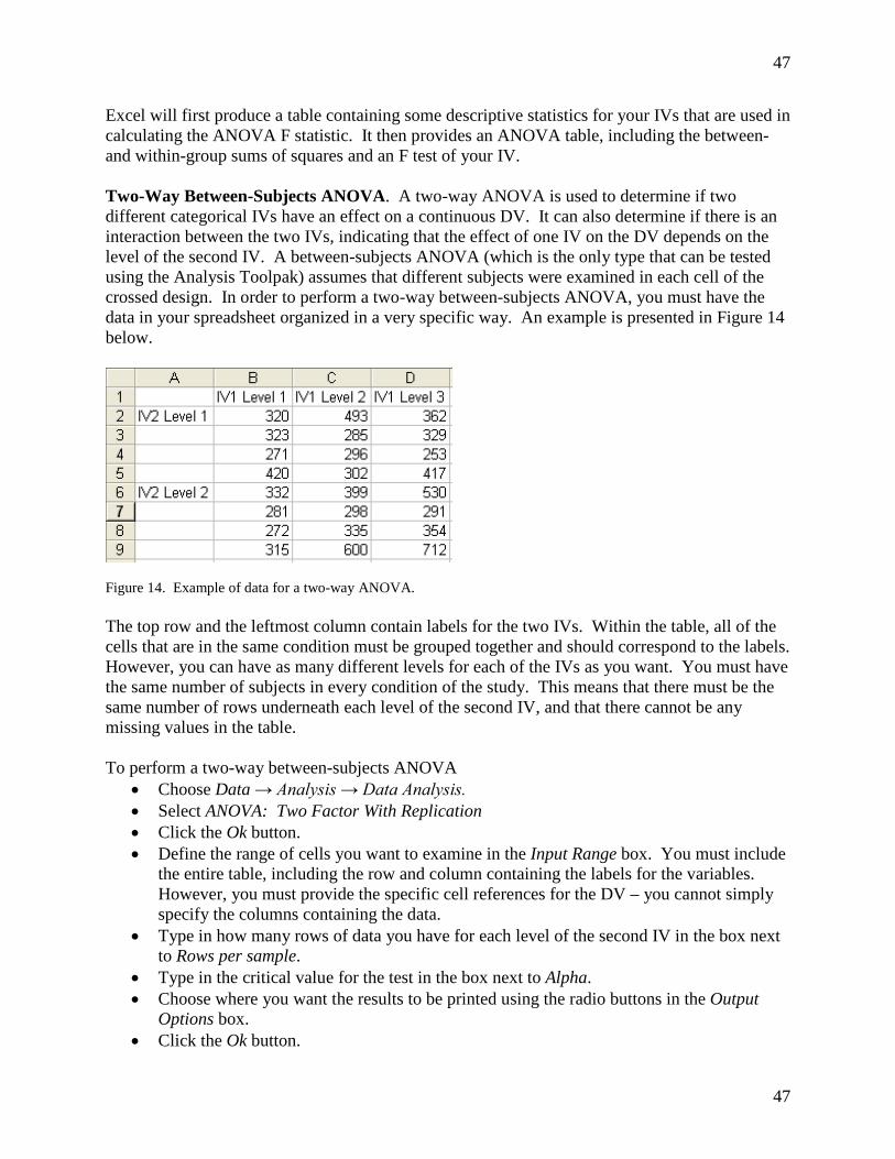
47
47
Excel will first produce a table containing some descriptive statistics for your IVs that are used in calculating the ANOVA F statistic. It then provides an ANOVA table, including the between- and within-group sums of squares and an F test of your IV. Two-Way Between-Subjects ANOVA. A two-way ANOVA is used to determine if two different categorical IVs have an effect on a continuous DV. It can also determine if there is an interaction between the two IVs, indicating that the effect of one IV on the DV depends on the level of the second IV. A between-subjects ANOVA (which is the only type that can be tested using the Analysis Toolpak) assumes that different subjects were examined in each cell of the crossed design. In order to perform a two-way between-subjects ANOVA, you must have the data in your spreadsheet organized in a very specific way. An example is presented in Figure 14 below.
Figure 14. Example of data for a two-way ANOVA. The top row and the leftmost column contain labels for the two IVs. Within the table, all of the cells that are in the same condition must be grouped together and should correspond to the labels. However, you can have as many different levels for each of the IVs as you want. You must have the same number of subjects in every condition of the study. This means that there must be the same number of rows underneath each level of the second IV, and that there cannot be any missing values in the table. To perform a two-way between-subjects ANOVA
• Choose Data → Analysis → Data Analysis. • Select ANOVA: Two Factor With Replication • Click the Ok button. • Define the range of cells you want to examine in the Input Range box. You must include
the entire table, including the row and column containing the labels for the variables. However, you must provide the specific cell references for the DV – you cannot simply specify the columns containing the data.
• Type in how many rows of data you have for each level of the second IV in the box next to Rows per sample.
• Type in the critical value for the test in the box next to Alpha. • Choose where you want the results to be printed using the radio buttons in the Output
Options box. • Click the Ok button.
48
48
The output will first provide descriptive statistics for all possible combinations of the levels of your two IVs. It follows this with an ANOVA table, including the between- and within-group sums of squares and an F test for your two IVs and the interaction term. Random Number Generation The Analysis Toolpak also has the ability to provide you with lists of random numbers. These random numbers can have several different properties. They can be drawn from a predefined distribution, such as uniform, normal, or Poisson distribution. Combined with a simple formula, you can use the uniform distribution generate a list of integers within a specified range. For example, you could ask Excel to generate a list of random numbers between 1 and 100. You can also draw random values from a customized distribution, where you specify a list of values and the probability that each will be chosen. Finally, you can also use the Toolpak to generate a nonrandom list of repeating numbers with properties that you define. To draw a list of random numbers from a predefined distribution
• Choose Data → Analysis → Data Analysis. • Select Random Number Generation. • Click the Ok button. • Type in the number of columns you want to fill with random numbers in the Number of
Variables box. • Type in how many random numbers you want placed in each column in the Number of
Random Numbers box. • Choose the distribution that you want to use from the Distribution pull-down menu. The
last two entries, Patterned and Discrete, are used to perform special tasks that we will discuss below.
• Each distribution will require to enter one or more values in the Parameters box that define the exact characteristic of the distribution used to generate the random numbers. For example, the normal distribution requires you to provide its mean and standard deviation.
• You can optionally enter a number in the Random Seed box if you want to be able to obtain the same random numbers at a later point in time. If you put different numbers in this box you will get different random lists. However, the same number always produces the exact same random output.
• Choose where you want the results to be printed using the radio buttons in the Output Options box.
• Click the Ok button. To generate a list of random integers
• Choose Data → Analysis → Data Analysis. • Select Random Number Generation. • Click the Ok button. • Type in the number of columns you want to fill with random numbers in the Number of
Variables box. • Type in how many random numbers you want placed in each column in the Number of
Random Numbers box.
49
49
• Select Uniform from the Distribution pull-down menu. • Define the upper and lower bounds of the distribution.
o Set the lower bound equal to the lowest integer you want to appear – 1. For example, if you want to generate a list of integers ranging from 1 to 100, you should set the lower bound equal to 0.
o Set the upper bound equal to the highest integer you want to appear. For example, if you want to generate a list of integers ranging from 1 to 100, you should set the upper bound equal to 100.
• Enter a number in the Random Seed box if you want to be able to obtain the same random numbers at a later point in time.
• Choose where you want the initial results to be printed using the radio buttons in the Output Options box. This will not be the final list of integers, but will be a list of continuous numbers that we use to generate our list of integers.
• Click the Ok button. Excel will now place a list of continuous numbers in the location you specify.
• For each column of random numbers you just created, create a new column in your spreadsheet defined by the formula =INT (cell containing a random number you just created) + 1. For example, if you put a random value in cell A5, you would use the formula =INT(A5) + 1 to obtain a corresponding random integer. The logic behind this formula is as follows.
o Your original list will contain numbers between (but not including) 0 and the upper bound of your range.
o The INT function rounds continuous numbers down to the nearest integer. This will generate a list of integers between your lower bound – 1 and your upper bound – 1.
o We add 1 to these values to make the list of random numbers between your lower bound and your upper bound.
To randomly draw items from a customized distribution
• Create a list of values and probabilities in an Excel spreadsheet o The first column contains the values as they should appear in your randomly
generated list. These must be numbers. o The second column, located directly to the right of the first column, contains the
probability that the value in the same row will be selected. The sum of all the probabilities must equal 1.
• Choose Data → Analysis → Data Analysis. • Select Random Number Generation. • Click the Ok button. • Type in the number of columns you want to fill with random numbers in the Number of
Variables box. • Type in how many random numbers you want placed in each column in the Number of
Random Numbers box. • Select Discrete from the Distribution pull-down menu. • Specify which cells describe your distribution in the Value and Probability Input Range
box. You must provide the specific cell boundaries – you cannot simply specify the two columns containing the values and their probabilities.
50
50
• Choose where you want the results to be printed using the radio buttons in the Output Options box.
• Click the Ok button. To generate a nonrandom repeating list of numbers
• Choose Data → Analysis → Data Analysis. • Select Random Number Generation. • Click the Ok button. • Select Patterned from the Distribution pull-down menu. • Specify which numbers you want included in the first row of the Parameters box.
o The first two boxes should contain the lower bound and upper bound of the list. o The third box specifies the which of the numbers within that range will be
included in the list. It will include the lower bound, (lower bound + step), (lower bound + 2*step), (lower bound + 3*step), and so on, up to the upper bound. The upper bound is always included, even if it is not a multiple of the step.
• Specify how many times Excel should print each number before it moves to the next one in the list in the second row of the Parameters box.
• Specify how many times you want the entire set repeated in the third row of the Parameters box.
• Choose where you want the results to be printed using the radio buttons in the Output Options box.
• Click the Ok button.


![[Jamie Oliver] Genial Kochen Mit Jamie Oliver. the(Bookos.org)](https://img.pdfslide.net/doc/110x75/5489a299b479590e7c8b46ca/jamie-oliver-genial-kochen-mit-jamie-oliver-thebookosorg.jpg)