9 SCIENTIFIC HIGHLIGHT OF THE MONTH

Exchange interactions, spin waves, and

transition temperatures in itinerant magnets

I. Turek,1,2,5 J. Kudrnovsky,3 V. Drchal,3 and P. Bruno4

1 Institute of Physics of Materials, Academy of Sciences of the Czech Republic,

Zizkova 22, CZ-61662 Brno, Czech Republic2 Department of Electronic Structures, Charles University in Prague,

Ke Karlovu 5, CZ-12116 Prague 2, Czech Republic3 Institute of Physics, Academy of Sciences of the Czech Republic,

Na Slovance 2, CZ-18221 Prague 8, Czech Republic4 Max-Planck-Institut fur Mikrostrukturphysik, Weinberg 2, D-06120 Halle, Germany

5 Center for Computational Materials Science, Technical University of Vienna,

Getreidemarkt 9/158, A-1060 Vienna, Austria

Abstract

The contribution reviews an ab initio two-step procedure to determine exchange inter-

actions, spin-wave spectra, and thermodynamic properties of itinerant magnets. In the

first step, the selfconsistent electronic structure of a system is calculated for a collinear spin

structure at zero temperature. In the second step, parameters of an effective classical Heisen-

berg Hamiltonian are determined using the magnetic force theorem and the one-electron

Green functions. The Heisenberg Hamiltonian and methods of statistical physics are em-

ployed in subsequent evaluation of magnon dispersion laws, spin-wave stiffness constants,

and Curie/Neel temperatures. Applicability of the developed scheme is illustrated by se-

lected properties of various systems like transition and rare-earth metals, disordered alloys

including diluted magnetic semiconductors, ultrathin films, and surfaces.

1 Introduction

The quantitative description of ground-state and finite-temperature properties of metallic sys-

tems represents a long-term challenge for solid state theory. Practical implementation of density

functional theory (DFT) [1, 2, 3] led to excellent parameter-free description of ground-state

112

properties of metallic magnets, including traditional bulk metals and ordered alloys as well as

systems without the perfect three-dimensional periodicity, like, e.g., disordered alloys, surfaces

and thin films. On the other hand, an accurate quantitative treatment of excited states and

finite-temperature properties of these systems remains an unsolved problem for ab initio theory

[4, 5, 6, 7] despite the formal extension of the DFT to time-dependent phenomena [8] and fi-

nite temperatures [9]. The usual local spin-density approximation (LSDA) [3] fails to capture

important features of excited states, in particular the magnetic excitations responsible for the

decrease of the magnetization with temperature and for the magnetic phase transition.

In developing a practical parameter-free scheme for the finite-temperature magnetism, one has

to rely on additional assumptions and approximations the validity of which has to be chosen

on the basis of physical arguments. The purpose of this contribution is to review theoretical

backgrounds, numerical aspects, and selected results of an approach formulated nearly two

decades ago [10, 11] (see Ref. [12] for a recent review), and applied by the present authors

to a number of qualitatively different systems [13, 14, 15, 16, 17, 18, 19, 20], including also

yet unpublished results. The review is organized as follows: Section 2 lists the underlying

physical concepts and approximations of the scheme and Section 3 deals with computational

details and specific problems related to its numerical implementation. Examples of applications

are given in Section 4: bulk transition metals (Section 4.1), rare-earth metals (Section 4.2),

disordered alloys (Section 4.3), diluted magnetic semiconductors (Section 4.4), two-dimensional

ferromagnets (Section 4.5), and surfaces of bulk ferromagnets (Section 4.6). Comparisons to

other authors using the same (or similar) approach are made throughout Section 4, while a

critical discussion of the scheme and a brief comparison to alternative approaches are left to the

last section (Section 5).

2 Formalism

It is well known that magnetic excitations in itinerant ferromagnets are basically of two different

types, namely, the Stoner excitations, in which an electron is excited from an occupied state of

the majority-spin band to an empty state of the minority-spin band and creates an electron-hole

pair of triplet spin, and the spin-waves, or magnons, which correspond to collective transverse

fluctuations of the magnetization direction. Near the bottom of the excitation spectrum, the

density of states of magnons is considerably larger than that of corresponding Stoner excitations

(associated with longitudinal fluctuations of the magnetization), so that the thermodynamics

in the low-temperature regime is completely dominated by magnons and Stoner excitations

can be neglected. Therefore it seems reasonable to extend this approximation up to the Curie

temperature and to derive an ab initio technique of finite-temperature magnetism by neglecting

systematically the Stoner excitations.

With thermodynamic properties in mind, we are primarily interested in the long-wavelength

magnons with the lowest energy. We adopt the adiabatic approximation [21] in which the

precession of the magnetization due to a spin-wave is neglected when calculating the associated

change of electronic energy. The condition of validity of this approximation is that the precession

time of the magnetization should be large as compared to characteristic times of electronic

113

motion, i.e., the hopping time of an electron from a given site to a neighboring one and the

precession time of the spin of an electron subject to the exchange field. In other words, the spin-

wave energies should be small as compared to the band width and to the exchange splitting. This

approximation becomes exact in the limit of long wavelength magnons, so that the spin-wave

stiffness constants calculated in this way are in principle exact.

This procedure corresponds to evaluation of changes of the total energy of a ferromagnet due to

infinitesimal changes of the directions of its local magnetic moments associated with individual

lattice sites R. The directions of the moments are specified by unit vectors eR. An exact

calculation of the total energy EeR of a prescribed spin configuration leads to the constrained

density functional theory [22], which allows to obtain the ground state energy for a system subject

to certain constraints. The latter are naturally incorporated into the DFT in terms of Lagrange

multipliers. In the present case, the constraint consists in imposing a given configuration of

spin-polarization directions, namely, along eR within the atomic (Wigner-Seitz) cell R. The

Lagrange multipliers can be interpreted as magnetic fields B⊥R constant inside the cells with

directions perpendicular to the unit vectors eR. Note that intracell non-collinearity of the

spin-polarization is neglected since we are primarily interested in low-energy excitations due to

intercell non-collinearity. In the so-called frozen-magnon approach, one chooses the constrained

spin-polarization configuration to be the one of a spin-wave with the wave vector q and computes

the spin-wave energy E(q) directly by employing the generalized Bloch theorem for a spin-spiral

configuration [23].

In a real-space approach, adopted here, one calculates directly the energy change associated with

a constrained rotation of the spin-polarization axes in two cells eR and eR′ . This represents

a highly non-trivial task which requires selfconsistent electronic structure calculations for non-

collinear spin-polarized systems without translational periodicity. Restriction to infinitesimal

changes of the moment directions, δuR = eR−e0, perpendicular to the direction of the ground-

state magnetization e0, leads to an expansion of EeR to second order in δuR of the form

[11, 24]

∆EδuR =∑

RR′

ARR′ δuR · δuR′ . (1)

This expression can be extended to finite changes of the moment directions using an effective

Heisenberg Hamiltonian (EHH)

HeffeR = −∑

RR′

JRR′ eR · eR′ . (2)

The constants JRR′ in Eq. (2), the pair exchange interactions, are parameters of the EHH which

satisfy JRR′ = JR′R and JRR = 0. They are related to the coupling constants ARR′ of Eq. (1)

by

ARR′ = −JRR′ + δRR′

(

∑

R′′

JR′′R

)

(3)

so that an important sum rule∑

R

ARR′ =∑

R′

ARR′ = 0 (4)

is satisfied which guarantees that the total energy remains invariant upon a uniform rotation of

the magnetization.

114

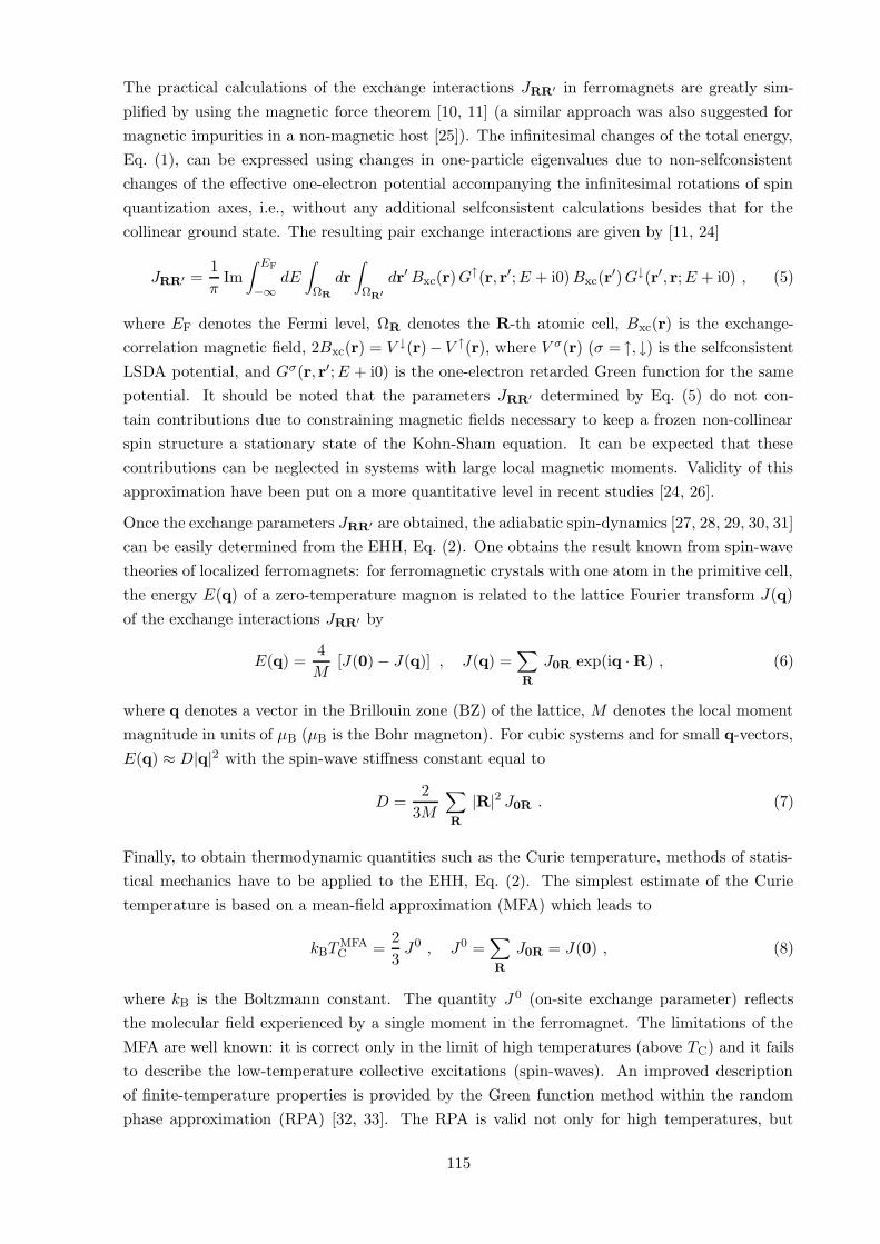
The practical calculations of the exchange interactions JRR′ in ferromagnets are greatly sim-

plified by using the magnetic force theorem [10, 11] (a similar approach was also suggested for

magnetic impurities in a non-magnetic host [25]). The infinitesimal changes of the total energy,

Eq. (1), can be expressed using changes in one-particle eigenvalues due to non-selfconsistent

changes of the effective one-electron potential accompanying the infinitesimal rotations of spin

quantization axes, i.e., without any additional selfconsistent calculations besides that for the

collinear ground state. The resulting pair exchange interactions are given by [11, 24]

JRR′ =1

πIm

∫ EF

−∞dE

∫

ΩR

dr

∫

ΩR′

dr′ Bxc(r) G↑(r, r′; E + i0) Bxc(r′) G↓(r′, r; E + i0) , (5)

where EF denotes the Fermi level, ΩR denotes the R-th atomic cell, Bxc(r) is the exchange-

correlation magnetic field, 2Bxc(r) = V ↓(r)− V ↑(r), where V σ(r) (σ = ↑, ↓) is the selfconsistent

LSDA potential, and Gσ(r, r′; E + i0) is the one-electron retarded Green function for the same

potential. It should be noted that the parameters JRR′ determined by Eq. (5) do not con-

tain contributions due to constraining magnetic fields necessary to keep a frozen non-collinear

spin structure a stationary state of the Kohn-Sham equation. It can be expected that these

contributions can be neglected in systems with large local magnetic moments. Validity of this

approximation have been put on a more quantitative level in recent studies [24, 26].

Once the exchange parameters JRR′ are obtained, the adiabatic spin-dynamics [27, 28, 29, 30, 31]

can be easily determined from the EHH, Eq. (2). One obtains the result known from spin-wave

theories of localized ferromagnets: for ferromagnetic crystals with one atom in the primitive cell,

the energy E(q) of a zero-temperature magnon is related to the lattice Fourier transform J(q)

of the exchange interactions JRR′ by

E(q) =4

M[J(0) − J(q)] , J(q) =

∑

R

J0R exp(iq · R) , (6)

where q denotes a vector in the Brillouin zone (BZ) of the lattice, M denotes the local moment

magnitude in units of µB (µB is the Bohr magneton). For cubic systems and for small q-vectors,

E(q) ≈ D|q|2 with the spin-wave stiffness constant equal to

D =2

3M

∑

R

|R|2 J0R . (7)

Finally, to obtain thermodynamic quantities such as the Curie temperature, methods of statis-

tical mechanics have to be applied to the EHH, Eq. (2). The simplest estimate of the Curie

temperature is based on a mean-field approximation (MFA) which leads to

kBTMFAC =

2

3J0 , J0 =

∑

R

J0R = J(0) , (8)

where kB is the Boltzmann constant. The quantity J 0 (on-site exchange parameter) reflects

the molecular field experienced by a single moment in the ferromagnet. The limitations of the

MFA are well known: it is correct only in the limit of high temperatures (above TC) and it fails

to describe the low-temperature collective excitations (spin-waves). An improved description

of finite-temperature properties is provided by the Green function method within the random

phase approximation (RPA) [32, 33]. The RPA is valid not only for high temperatures, but

115

also at low temperatures, and it describes correctly the spin-waves. In the intermediate regime

(around TC), it represents a rather good approximation which may be viewed as an interpolation

between the high and low temperature regimes. The RPA formula for the Curie temperature is

given by(

kBTRPAC

)−1=

3

2

1

N

∑

q

[

J0 − J(q)]−1

, (9)

where N denotes the number of q-vectors used in the BZ-average. It can be shown that T RPAC is

always smaller than T MFAC . It should be noted, however, that both the MFA and the RPA fail

to describe correctly the critical behavior and yield in particular incorrect critical exponents.

Finally, the Curie temperature can also be estimated purely numerically by employing the

method of Monte Carlo simulations applied to the EHH. This approach is in principle exact but

its application to real itinerant systems requires inclusion of a sufficient number of neighboring

shells due to long-ranged interactions JRR′ (see Section 3.2).

3 Numerical implementation

3.1 Selfconsistent electronic structure

Efficient evaluations of the pair exchange interactions, Eq. (5), require a first-principle tech-

nique which provides the one-electron Green function in the real space. The results reported

here are based on selfconsistent LSDA calculations using the all-electron non-relativistic (scalar-

relativistic) tight-binding linear muffin-tin orbital (TB-LMTO) method and the atomic-sphere

approximation (ASA) [34, 35, 36], with the exchange-correlation potential parametrized accord-

ing to Ref. [37]. The energy integrals over the occupied part of the valence band were expressed

as integrals over an energy variable along a closed path C starting and ending at the Fermi en-

ergy (with the occupied part of the valence band lying inside C). The integrals were numerically

evaluated using the Gaussian quadrature method [35, 36]. Other Green function techniques, es-

pecially the the Korringa-Kohn-Rostoker (KKR) method [38, 39], are equally suitable in the

present context.

Within the ASA, the Green function for a closely packed solid can be written in the form [35, 40]

(the spin index σ is omitted for brevity in Section 3.1)

G(r + R, r′ + R′; z) = − δRR′

∑

L

ϕRL(r<, z) ϕRL(r>, z)

+∑

LL′

ϕRL(r, z) GRL,R′L′(z) ϕR′L′(r′, z) . (10)

In Eq. (10), the variables r, r′ refer to positions of points inside the individual atomic spheres,

z denotes a complex energy variable, the symbol r< (r>) denotes that of the vectors r, r′ with

the smaller (larger) modulus, and L,L′ are the angular momentum indices, L = (`,m). The

functions ϕRL(r, z) and ϕRL(r, z) denote, respectively, properly normalized regular and irregular

solutions of the Schrodinger equation for the spherically symmetric potential inside the R-

th atomic sphere. All multiple-scattering effects are contained in the Green function matrix

GRL,R′L′(z) which is given in terms of the potential functions PR`(z) and the structure constants

116

SRL,R′L′ of the LMTO method by

GRL,R′L′(z) = λR`(z) δRL,R′L′ + µR`(z) gRL,R′L′(z) µR′`′(z) , (11)

where the quantities on the r.h.s. are defined as

µR`(z) =√

PR`(z) , λR`(z) = − 1

2

PR`(z)

PR`(z),

gRL,R′L′(z) =

[P (z) − S]−1

RL,R′L′. (12)

In the last equation, the symbol P (z) denotes a diagonal matrix of potential functions defined as

PRL,R′L′(z) = PR`(z) δRL,R′L′ and an overdot means energy derivative. The matrix gRL,R′L′(z)

will be referred to as the auxiliary (or KKR-ASA) Green function. The quantities PR`(z),

µR`(z), λR`(z), SRL,R′L′ , and gRL,R′L′(z) can be expressed in any particular LMTO represen-

tation (canonical, screened); the resulting Green function matrix, Eq. (11), the Green function,

Eq. (10), and all derived physical quantities are invariant with respect to this choice. However,

the most screened (tight-binding) representation is the best suited for most calculations and

it has been employed in the present implementation. The energy dependence of the potential

functions PR`(z) is parametrized in terms of three standard potential parameters, i.e., with the

second-order accuracy [34, 35].

3.2 Parameters of the classical Heisenberg Hamiltonian

Substitution of the Green function Gσ(r, r′; z) in the ASA (Section 3.1) into Eq. (5) yields an

expression suitable for computations [11, 12, 14], namely,

JRR′ = − 1

8πi

∫

CtrL

[

∆R(z) g↑RR′(z) ∆R′(z) g↓R′R(z)]

dz ,

∆R(z) = P ↑R(z) − P ↓

R(z) , (13)

where trL denotes the trace over the angular momentum index L and energy integration is

performed along the contour C described in Section 3.1. The quantities gσRR′(z) (σ = ↑, ↓) denote

site-off-diagonal blocks of the auxiliary Green-function matrices with elements gσRL,R′L′(z) while

∆R(z) are diagonal matrices related to the potential functions P σR`(z). The diagonal elements

of ∆R(z) play a role of energy- and `-dependent exchange splittings on individual atoms while

the expression (13) for the exchange interactions JRR′ has a form of a bare static transversal

susceptibility.

Well converged calculations of the exchange interactions JRR′ for bulk metals with perfect

translational symmetry for distances d = |R − R′| up to ten lattice constants a require high

accuracy of the full BZ-averages (inverse lattice Fourier transforms) defining the site-off-diagonal

blocks gσRR′(z) [35, 36]. In particular, we have used typically a few millions of k-points in the

full BZ for the energy point on the contour C closest to the Fermi energy, and the number of k-

points then progressively decreased for more distant energy points [14, 17]. A typical evaluation

of exchange interactions requires about two hours on P4-based personal computers.

The calculated Heisenberg exchange parameters for bcc Fe (with experimental value of its lattice

constant) are shown in Fig. 1. One can see dominating ferromagnetic interactions for the first

117

and second nearest-neighbor shells followed by weaker interactions of both signs and decreasing

magnitudes for bigger distances d = |R −R′| (Fig. 1, left panel). The same qualitative features

were found for other 3d ferromagnets: fcc Co, fcc Ni [14] and hcp Co [18].

-0.5

0.0

0.5

1.0

1.5

2.0

1 2 3 4 5 6 7 8 9 10

J (

mR

y)

d/a

Fe bcc

-6-5

-4-3-2-101

234

56

1 2 3 4 5 6 7 8 9 10

(d/a

)3 J (

mR

y)

d/a

Fe bcc

Figure 1: Exchange interactions JRR′ for bcc Fe as a function of the distance |R − R′| = d

without (left panel) and with (right panel) a prefactor d3.

An analysis of the exchange interactions JRR′ , Eq. (13), in the limit of large distances d =

|R − R′| has been given in Ref. [14] for a a single-band model using the stationary-phase ap-

proximation [41]. For a weak ferromagnet, one reveals a characteristic Ruderman-Kittel-Kasuya-

Yoshida (RKKY) asymptotic behavior

JRR′ ∝sin[(

k↑F + k↓

F

)

· (R − R′) + Φ]

|R − R′|3 , (14)

where kσF is a Fermi wave vector in a direction such that the associated group velocity is parallel

to R − R′, and Φ denotes a phase factor. The exchange interaction according to Eq. (14) has

an oscillatory character with an envelope decaying as |R − R′|−3. On the other hand, for a

strong ferromagnet with a fully occupied majority band the corresponding Fermi wave vector is

imaginary, namely, k↑F = i K↑

F, and one obtains an exponentially damped RKKY behavior

JRR′ ∝sin[

k↓F · (R − R′) + Φ

]

exp[

−K↑F · (R − R′)

]

|R − R′|3 . (15)

The qualitative features of these RKKY-type oscillations will not be changed in realistic ferro-

magnets. This is illustrated for bcc Fe (weak ferromagnet) in Fig. 1 (right panel) which proves

undamped oscillations of the quantity |R − R′|3JRR′ . It should be noted that due to the sp-d

hybridization no itinerant ferromagnet is a truly strong ferromagnet – the only exceptions are

half-metallic ferromagnets.

3.3 Magnetic properties from the Heisenberg Hamiltonian

The RKKY-like asymptotic behavior, Eq. (14), leads to numerical difficulties in calculations of

the magnon spectra and the spin-wave stiffness constants. The lattice Fourier transform of the

118

exchange interactions, Eq. (6), is not an absolutely convergent sum and its convergence with

respect to the number of shells included has to be carefully checked (see Section 4.1). Note,

however, that the lattice sum over |J0R|2 does converge so that J(q) is defined unambiguously

in the L2 sense.

0 2 4 6 8dmax/a

0

200

400

600

800

1000

D [m

eV.A

2]

η = 0.0

η = 0.2

η = 0.4

η = 0.6

η = 0.8

Ni

Figure 2: Spin-wave stiffness of fcc Ni as a function of dmax (in units of lattice constant) for

various values of the damping factor η.

The lattice sum for the spin-wave stiffness constant, Eq. (7), is not convergent at all, and the

values of D as functions of a cut-off distance dmax exhibit undamped oscillations for all three

cubic 3d ferromagnets [14]. To resolve this difficulty we suggested to regularize the original

expression, Eq. (7), by replacing it by the formally equivalent expression which is, however,

numerically convergent

D(η) =2

3Mlim

dmax→∞

∑

|R|<dmax

|R|2 J0R exp(−η|R|/a) ,

D = limη→0

D(η) , (16)

where a is the lattice constant. The quantity η plays a role of a damping parameter which makes

the lattice sum absolutely convergent as it is seen from Fig. 2 for the case of fcc Ni.

It can be shown that the quantity D(η) is an analytical function of the variable η for any value

η > 0 and it can be extrapolated to the value η = 0. We therefore perform calculations for a set

of values η ∈ (ηmin, ηmax) for which D(η) is a smooth function with a well defined limit for large

dmax. The limit η → 0 is then determined at the end of calculations by a quadratic least-square

extrapolation method. The procedure is illustrated in Fig. 3 for the cubic Fe, Co and Ni. Note

that these convergence problems are less serious in half-metallic magnets due to the exponential

damping described by Eq. (15).

Direct calculations of the Curie temperatures in the MFA according to Eq. (8) face convergence

problems similar to the magnon spectra. Alternatively, one can evaluate the on-site exchange

parameter J0 using a sum rule valid also for systems without translational periodicity [11]:

J0R =

∑

R′

JRR′ =1

8πi

∫

CtrL

[

∆R(z)(

g↑RR(z) − g↓RR(z))

119

0 0.2 0.4 0.6 0.8 1η

0

200

400

600

800

D [m

eV.A

2]

Fe

Ni

Co

Figure 3: Spin-wave stiffness coefficients D(η) for bcc Fe, fcc Co, and fcc Ni as a function of the

parameter η (open symbols) and extrapolated values for η = 0 (filled symbols). The solid line

indicates the quadratic fit function used for extrapolation.

+ ∆R(z) g↑RR(z) ∆R(z) g↓RR(z)]

dz . (17)

This sum rule involves only the site-diagonal blocks of the auxiliary Green functions and its

reliable evaluation for perfect crystals requires only a few thousands of k-points in the irreducible

part of the BZ, i.e., accuracy usual in most selfconsistent LSDA calculations.

Another numerical problem is encountered in computations of the Curie temperature in the

RPA due to the singularity of the averaged function in Eq. (9) for |q| → 0. We have therefore

calculated T RPAC using the expression

(

kBTRPAC

)−1= − 3

2limz→0

Gm(z) , Gm(z) =1

N

∑

q

[

z − J0 + J(q)]−1

, (18)

where z is a complex energy variable and the quantity Gm(z) is a magnon Green function

corresponding (up to the prefactor 4/M) to the magnon dispersion law, Eq. (6). The magnon

Green function was evaluated for energies z in the complex energy plane and its value for z = 0

was obtained using an analytical continuation technique [42].

4 Applications

4.1 Transition metals

Calculated magnon energy spectra E(q) for bcc Fe are presented in Fig. 4. Corresponding plots

of E(q) for fcc Co and Ni [14] exhibit parabolic, almost isotropic behavior for long wavelengths.

On the contrary, in bcc Fe we observe some anisotropy of E(q), i.e., E(q) increases faster along

the Γ−N direction and more slowly along the Γ−P direction. In agreement with Refs. [27, 43, 44]

we observe a local minima around the point H along Γ−H and H−N directions in the range of

short wavelengths. They are indications of the so-called Kohn anomalies which are due to long-

range interactions mediated by the RKKY interactions similarly like Kohn-Migdal anomalies in

120

phonon spectra are due to long-range interactions mediated by Friedel oscillations. It should be

mentioned that minima in dispersion curve of bcc Fe appear only if the summation in Eq. (6)

is done over a sufficiently large number of shells, in the present case for more than 45 shells.

0

200

400

600

Ene

rgy

[meV

]

N P H NΓ Γ

Fe

Figure 4: Magnon dispersion law along high-symmetry lines in the Brillouin zone of bcc Fe

compared to experiment (filled circles: pure Fe at 10 K [45], empty squares: Fe(12% Si) at room

temperature [46]).

Present results for dispersion relations compare well with available experimental data of mea-

sured spin-wave spectra for Fe and Ni [45, 46, 47]. For low-lying part of spectra there is also a

good agreement of present results for dispersion relations with those of Refs. [27, 44] obtained

using the frozen-magnon approach. There are, however, differences for a higher part of spectra,

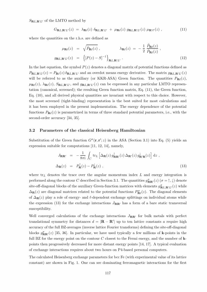
in particular for the magnon bandwidth of bcc Fe which can be identified with the value of E(q)

evaluated at the high-symmetry point q = H in the bcc BZ. The origin of this disagreement is

unclear. We have carefully checked the convergence of the magnon dispersion laws E(q), see

Fig. 5, with the number of shells included in Eq. (6) and it was found to be weak for 50 – 70

shells and more, i.e., for the cut-off distance dmax ≥ 6a.

The results for spin stiffness coefficient D calculated for the three cubic ferromagnetic metals

are summarized in Tab. 1 together with available experimental data [48, 49, 50]. There is a

reasonable agreement between theory and experiment for bcc Fe and fcc Co but the theoretical

values of D are considerably overestimated for fcc Ni. It should be noted that measurements

refer to the hcp Co while the present calculations were performed for fcc Co. A similar agreement

between calculated and measured spin-wave stiffness constants was obtained by Halilov et al.

[27] using the frozen-magnon approach. Our results are also in accordance with those obtained

by van Schilfgaarde and Antropov [44] who used the spin-spiral calculations to overcome the

problem of evaluation of D from Eq. (7). On the other hand, this problem was overlooked in

Refs. [11, 51, 52] so that a good agreement of D, calculated for a small number of coordination

shells, with experimental data seems to be fortuitous. Finally, the results of Brown et al. [53]

obtained by the layer KKR method in the frozen potential approximation are underestimated

for all metals and the best agreement is obtained for Ni.

Calculated values of Curie temperatures for both the MFA and RPA as well as corresponding

121

0

100

200

300

400

500

600

700

0 2 4 6 8 10

Mag

non

band

wid

th (

meV

)

d /amax

bcc Fe

Figure 5: The magnon bandwidth for bcc Fe as a function of the cut-off distance dmax. The

bandwidth is identified with the magnon energy at the high-symmetry point H in the bcc

Brillouin zone.

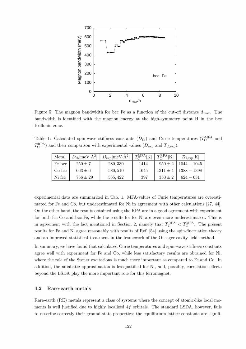
Table 1: Calculated spin-wave stiffness constants (Dth) and Curie temperatures (T MFAC and

TRPAC ) and their comparison with experimental values (Dexp and TC,exp).

Metal Dth[meV·A2] Dexp[meV·A2] TMFAC [K] TRPA

C [K] TC,exp[K]

Fe bcc 250 ± 7 280, 330 1414 950 ± 2 1044 − 1045

Co fcc 663 ± 6 580, 510 1645 1311 ± 4 1388 − 1398

Ni fcc 756 ± 29 555, 422 397 350 ± 2 624 − 631

experimental data are summarized in Tab. 1. MFA-values of Curie temperatures are overesti-

mated for Fe and Co, but underestimated for Ni in agreement with other calculations [27, 44].

On the other hand, the results obtained using the RPA are in a good agreement with experiment

for both fcc Co and bcc Fe, while the results for fcc Ni are even more underestimated. This is

in agreement with the fact mentioned in Section 2, namely that T RPAC < TMFA

C . The present

results for Fe and Ni agree reasonably with results of Ref. [54] using the spin-fluctuation theory

and an improved statistical treatment in the framework of the Onsager cavity-field method.

In summary, we have found that calculated Curie temperatures and spin-wave stiffness constants

agree well with experiment for Fe and Co, while less satisfactory results are obtained for Ni,

where the role of the Stoner excitations is much more important as compared to Fe and Co. In

addition, the adiabatic approximation is less justified for Ni, and, possibly, correlation effects

beyond the LSDA play the more important role for this ferromagnet.

4.2 Rare-earth metals

Rare-earth (RE) metals represent a class of systems where the concept of atomic-like local mo-

ments is well justified due to highly localized 4f orbitals. The standard LSDA, however, fails

to describe correctly their ground-state properties: the equilibrium lattice constants are signifi-

122

cantly smaller than the experimental ones due to an overestimated 4f -contribution to cohesion,

and the ground-state magnetic structures in the LSDA are qualitatively wrong as well. In the

case of Gd in hcp structure, the antiferromagnetic (AFM) stacking of the (0001) atomic planes

was predicted [55] in contrast to the observed ferromagnetic (FM) state [56]. The most sophis-

ticated methods beyond the LSDA, which improve the situation, take explicitly into account

the on-site Coulomb interaction of the 4f electrons, like the LSDA+U scheme [57, 58] and the

self-interaction corrected (SIC) LSDA approach [59, 60]. Ground-state magnetic structures of

4f electron systems are often non-collinear and incommensurate with the underlying chemical

unit cell [56] which presents another complication for ab initio techniques.

We have treated two RE metals, namely, hcp Gd [17] and bcc Eu [18], in a simplified manner

taking the 4f states as a part of the atomic core (with the majority 4f level occupied by 7

electrons and the minority 4f level empty). The other valence orbitals were included in the

standard LSDA. This ‘open-core’ approach was often employed in selfconsistent spin-polarized

calculations of RE-based systems during the last decade [60, 61, 62, 63] and it yielded the correct

FM structure of hcp Gd. The theoretical equilibrium Wigner-Seitz radii s (sGd = 3.712 a.u.

with the experimental value of c/a = 1.597, sEu = 4.190 a.u.) are only slightly smaller than

the experimental values (sGd = 3.762 a.u., sEu = 4.238 a.u.). Different spin configurations were

considered for both metals: FM, AFM, and the disordered local moment (DLM) state [21].

The theoretical equilibrium values of s are nearly insensitive to the spin structures and the FM

ground state of Gd exhibits a non-negligible energy separation from the AFM and DLM states

in contrast to the bcc Eu, where the DLM state is slightly more stable than the FM state.

0.0

0.1

0.2

1 2 3 4 5 6

J (m

Ry)

d/a

Gd

0.0

0.1

0.2

1 2 3 4 5 6

J (m

Ry)

d/a

Eu

Figure 6: Exchange interactions JRR′ for hcp Gd (left panel) and bcc Eu (right panel) as

functions of the distance |R − R′| = d. The crosses and squares in the left panel refer to pairs

of sites R, R′ lying in even (AA) and odd (AB) hcp(0001) planes, respectively.

The exchange interactions in Gd and Eu, derived for the FM state and the theoretical equilibrium

Wigner-Seitz radius s, are shown in Fig. 6. Their distance-dependence is qualitatively similar

to the 3d transition metals, the magnitudes of the dominating nearest-neighbor interactions are,

however, smaller by a factor of five, cf. Fig. 1. Moreover, as illustrated in Fig. 7 by calculating

the on-site exchange parameter J 0 as a function of the cut-off distance dmax used in the real-

space sum in Eq. (8), there is a profound difference between the two 4f metals concerning the

123

oscillating interactions of more distant atoms. In the hcp Gd, they are not strong enough to

destroy the FM spin structure, as indicated by the positive converged value of J 0. Note that

the negative exchange interaction between the second Gd nearest neighbors is in qualitative

agreement with experiment [64]. On the other hand, the contribution of more distant sites to

J0 is very important in the case of bcc Eu and it yields for the converged quantity a negligible

resulting value (J0 = −0.03 mRy). Such a situation indicates an instability of the FM state

with respect to a more complicated spin structure. This feature agrees qualitatively with an

experimentally observed helical spin structure, the wave vector of which lies along the Γ − H

direction in the bcc BZ [65, 66].

1.0

1.5

2.0

2.5

3.0

3.5

1 2 3 4 5 6 7

Gd

J0 (m

Ry)

-0.5

0.0

0.5

1.0

1.5

2.0

1 2 3 4 5 6 7 8 9 10

J0 (m

Ry)

dmax/a

Eu

Figure 7: The on-site exchange parameter J 0 for hcp Gd (top panel) and bcc Eu (bottom panel)

as a function of the cut-off distance dmax used in the real-space summation in Eq. (8). The

horizontal lines mark exact values of J 0 obtained from the sum rule, Eq. (17).

Table 2: Calculated magnetic transition temperatures (T MFA and TRPA) and their comparison

with experimental values (Texp) for hcp Gd (Curie temperature) and bcc Eu (Neel temperature).

Calculations were performed with experimental values of lattice parameters.

Metal T MFA[K] TRPA[K] Texp[K]

Gd hcp 334 300 293

Eu bcc 151 111 91

Calculations of the magnon spectra and the Curie temperature for hcp Gd require a trivial

generalization of Eqs. (6, 9) to the case of two equivalent atoms in the hcp unit cell [67]. The

resulting Curie temperatures are given in Tab. 2 together with the experimental value [56] while a

comparison of the calculated magnon dispersion law with experiment [56] is presented in Fig. 8.

The theoretical magnon spectra included finite temperature of the experiment (T = 78 K)

124

which leads within the RPA to a simple rescaling of the magnon energies proportionally to the

temperature-dependent average magnetization [32]. The latter dependence was calculated in

the RPA from the classical EHH [67].

0

10

20

30

Γ M K Γ A

Gd

Mag

non

ener

gy (

meV

)

Figure 8: Magnon dispersion law along high-symmetry lines in the Brillouin zone of hcp Gd

calculated for T = 78 K (lines) and compared to experiment (filled circles - Ref. [56]).

The calculated magnon energies are higher than experimental. A recent theoretical study by

Halilov et al. [43, 62] revealed that this effect can be partly explained by assumed collinearity

between the localized 4f -moment and the valence part of the local moment. Inclusion of a

possible non-collinearity between the localized and itinerant moments leads to a softening of the

magnon energies, reducing them by a factor of 1.5 in the upper part of the spectrum. However,

the lower part of the spectrum that is more important for an RPA estimation of the Curie

temperature is less influenced by the non-collinearity. On the other hand, the calculated Curie

temperatures both in the MFA and in the RPA agree very well with experiment (Tab. 2). This

degree of agreement proves that the present approach based on interatomic exchange interactions

represents a better starting point to RE magnetism than a theory based on intraatomic exchange

integrals formulated in Ref. [68]. The latter scheme provided values of the Curie temperature

for Gd in a wide interval between 172 K and 1002 K, depending on further approximations

employed.

Determination of the magnetic ground state of Eu from the EHH, Eq. (2), is a difficult task

in view of the highly-dimensional manifold of a priori possible states as well as a number of

qualitatively different spin structures encountered in RE-based systems [56]. Here we consider

only spin spirals specified by a single q-vector as

eR = (sin(q · R), 0, cos(q · R)) , (19)

since the spin structure observed for bcc Eu at low temperatures belongs to this class [65, 66].

The minimum of the Hamiltonian Heff corresponds then to the maximum of the lattice Fourier

transform J(q), Eq. (6). A scan over the whole BZ reveals that the absolute maximum of J(q)

(for the theoretical equilibrium Wigner-Seitz radius s = 4.19 a.u.) is obtained for a vector q = Q

on the Γ − H line, namely, at Q = (1.69, 0, 0) a−1 , see Fig. 9. The magnitude of Q determines

the angle ω between magnetic moments in the neighboring (100) atomic layers. In the present

case, it is equal to ω = 48. Similar values were obtained for the experimental value of the

125

Wigner-Seitz radius sexp = 4.238 a.u.: Q = (1.63, 0, 0) a−1 , ω = 47. Both data sets are in

surprising agreement with experimental results which report the spin-spiral q-vector inside the

Γ − H line and the angle per layer equal to ωexp = 49 [65] and ωexp = 47.6 ± 1.2 [66].

-1.5

-1.0

-0.5

0.0

0.5

1.0

1.5

J(q)

(m

Ry)

Eu

Γ N P Γ H N

Figure 9: The lattice Fourier transform J(q) of the exchange interactions in bcc Eu along

high-symmetry lines in the Brillouin zone.

The resulting maximum J(Q) can be used to get the Neel temperature in the MFA in complete

analogy to Eq. (8) [56]:

kBTMFAN =

2

3J(Q) , (20)

whereas the RPA leads to the following modification of Eq. (9) [32, 69]:

(

kBTRPAN

)−1=

3

4

1

N

∑

q

[J(Q) − J(q)]−1 + [W (q, Q)]−1

,

W (q, Q) = J(Q) − 1

2J(q + Q) − 1

2J(q − Q) . (21)

Both theoretical values and the experimental Neel temperature are given in Tab. 2. The MFA-

value is substantially higher than experiment while the RPA reduces the theoretical value of TN

significantly so that a good agreement with experiment is obtained.

4.3 Substitutionally disordered alloys

The present real-space approach to exchange interactions can be generalized to substitutionally

disordered alloys either by using a supercell technique or by combining it with the coherent-

potential approximation (CPA). Both alternatives have their own merits and drawbacks. The

CPA takes properly into account the effects of finite lifetime of electronic states due to disorder

but it has difficulties to include effects of varying local environments as well as of short-range

order (both chemical and magnetic) on electronic properties.

In the following, we sketch the modification of the expression for the exchange interactions,

Eq. (13), to a random alloy within the LMTO-CPA formalism [35, 36, 70]. We assume that the

lattice sites R are randomly occupied by alloy components Q = A,B, . . ., with concentrations

cQR. We neglect any correlations between occupations of different lattice sites and we neglect

local environment effects, i.e., the LSDA selfconsistent potentials inside R-th cell depend solely

on occupation of the site R by an atom Q = A,B, . . ..

126

The CPA-configurational average of the auxiliary Green function, Eq. (12), can be written as

〈gRR′(z)〉 = gRR′(z) =

[P(z) − S]−1

RR′, (22)

where the spin index σ is omitted, S is the structure constant matrix and P(z) is a non-

random site-diagonal matrix of coherent potential functions PR(z) attached to individual lattice

sites which describe effective atoms forming an effective CPA medium. The coherent potential

functions satisfy a set of selfconsistency conditions (Soven equation) which guarantees that

average single-site scattering due to real atoms with respect to the effective medium vanishes.

The CPA leads also to conditional averages of individual blocks of the Green functions. The

site-diagonal block gRR(z) of the Green function averaged over all alloy configurations with site

R occupied by an atom Q is given by

gQRR(z) = gRR(z) fQ

R(z) = fQR(z) gRR(z) , (23)

where the prefactors fQR(z) and fQ

R(z) are defined as

fQR(z) =

1 +[

PQR (z) −PR(z)

]

gRR(z)−1

,

fQR(z) =

1 + gRR(z)[

PQR (z) −PR(z)

]−1. (24)

Similarly, the site-off-diagonal block gRR′(z) averaged over all alloy configurations with two sites

R 6= R′ occupied respectively by atomic species Q and Q′ is given by

gQQ′

RR′(z) = fQR(z) gRR′(z) fQ′

R′ (z) . (25)

Derivation of the conditionally averaged pair exchange interaction between two sites R 6= R ′

occupied respectively by components Q and Q′ can be performed similarly like in the case

without substitutional randomness by employing the magnetic force theorem [11] and the so-

called vertex-cancellation theorem [71, 72]. It leads to an expression

JQQ′

RR′ = − 1

8πi

∫

CtrL

[

∆QR(z) gQQ′,↑

RR′ (z) ∆Q′

R′(z) gQ′Q,↓R′R (z)

]

dz ,

∆QR(z) = P Q,↑

R (z) − P Q,↓R (z) , (26)

which is fully analogous to Eq. (13). The conditional average of the on-site exchange interaction,

Eq. (17), yields a formula

J0,QR =

1

8πi

∫

CtrL

[

∆QR(z)

(

gQ,↑RR(z) − gQ,↓

RR(z))

+ ∆QR(z) gQ,↑

RR(z) ∆QR(z) gQ,↓

RR(z)]

dz . (27)

It should be noted, however, that the sum rule for the averaged pair and on-site interactions,

J0,QR =

∑

R′Q′

JQQ′

RR′ cQ′

R′ , (28)

which can be easily obtained from the corresponding sum rule, Eq. (17), valid for any configu-

ration of the alloy, is not exactly satisfied by the expressions (26) and (27). According to our

127

experience, the two sides of Eq. (28) deviate up to 15% for typical binary transition-metal alloys

(FeV, FeAl). This violation of an important sum rule indicates that vertex corrections must

be taken into account in averaging exchange interactions in random alloys. On the other hand,

the small relative difference of both sides of the sum rule (28) proves that the role of vertex

corrections for exchange interactions is less significant than in transport properties, as argued

in Ref. [73].

Let us now consider the case of two isolated impurities in a non-magnetic host. The exchange

interaction between impurity sites R 6= R′ can be calculated exactly and compared to the low-

concentration limit of the CPA expression, Eq. (26). The latter case corresponds to a binary

alloy with cAR → 0 and cB

R → 1 for all lattice sites, with the coherent potential functions

PσR(z) → P 0

R(z) where P 0R(z) = P B

R (z) are the non-spin-polarized host potential functions, and

with the average Green function substituted by that of the non-random host, gσRR′(z) → g0

RR′(z).

Direct calculation of the exchange interaction for two impurities embedded in a crystal gives a

result (the so-called two-potential formula [74]) which differs from the low-concentration limit

of the CPA expression by matrix quantities XσRR′(z) defined in terms of single-site t-matrices

of impurities τσR(z) as

XσRR′(z) =

(

1 − g0RR′(z) τσ

R′(z) g0R′R(z) τσ

R(z))−1

,

τσR(z) =

[

PA,σR (z) − P 0

R(z)]

1 + g0RR(z)

[

PA,σR (z) − P 0

R(z)]−1

. (29)

The quantities XσRR′(z) – which enter the impurity-impurity interaction as multiplicative pref-

actors at the site-off-diagonal blocks g0RR′(z) of the host Green function – describe multiple

scatterings of electrons between the two impurity sites; their absence in the exchange interac-

tion derived from the low-concentration limit of Eq. (26) reflects a systematic neglect of such

multiple-scattering processes in single-site theories like the CPA.

-0.5

0.0

0.5

1.0

1.5

2.0

1 2 3 4 5 6 7 8 9 10

J (

mR

y)

d/a

Fe - 20% Al

-1.0

-0.5

0.0

0.5

1.0

1.5

1 2 3 4 5 6 7 8 9 10

(d/a

)3 J (

mR

y)

d/a

Fe - 20% Al

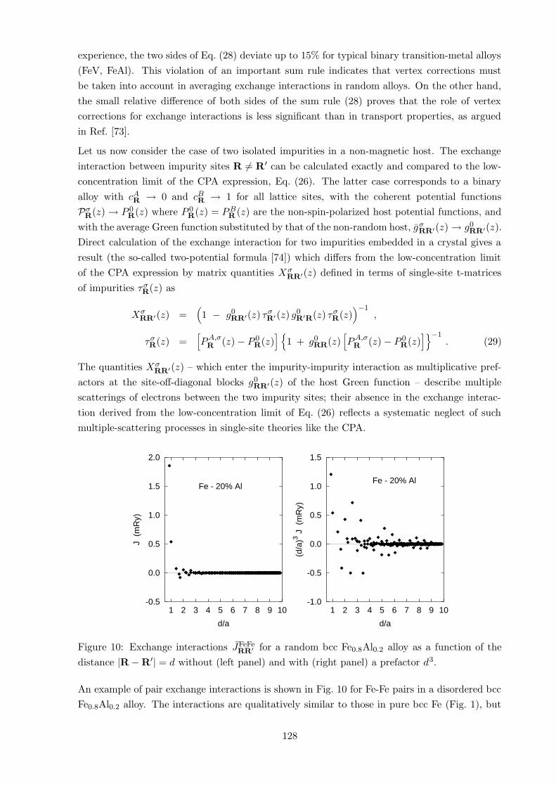
Figure 10: Exchange interactions JFeFeRR′ for a random bcc Fe0.8Al0.2 alloy as a function of the

distance |R − R′| = d without (left panel) and with (right panel) a prefactor d3.

An example of pair exchange interactions is shown in Fig. 10 for Fe-Fe pairs in a disordered bcc

Fe0.8Al0.2 alloy. The interactions are qualitatively similar to those in pure bcc Fe (Fig. 1), but

128

a more careful analysis of the long-distance behavior reveals an exponentially damped RKKY-

like oscillations (Fig. 10, right panel). This feature can be explained by damping of electron

states due to the alloy disorder which leads to exponential decay of site-off-diagonal blocks of

the averaged Green functions gσRR′(z) with increasing distance |R−R′|. It should be mentioned

that this exponential damping refers only to averaged exchange interactions in contrast to those

in each alloy configuration which exhibit a much slower decay for large interatomic separations

(see Ref. [73] and references therein).

Calculation of magnon spectra in disordered alloys represents a non-trivial task since the cor-

responding equation of motion for the two-time Green function for spin operators, obtained

from the standard decoupling procedure for higher-order Green functions [32], contains a more

complicated type of disorder than purely diagonal disorder. The magnons (and also phonons)

in random alloys are featured by simultaneous presence of diagonal, off-diagonal and environ-

mental disorder; the latter is closely related to the Goldstone theorem for these excitations.

An extension of the CPA to this case has been studied since early 1970’s. Two most recent

approaches are based on a cumulant expansion [75] and on an augmented-space formalism [76];

the former scheme is combined with the RPA and provides a value for the Curie temperature.

Both formulations are rather complicated which allowed to perform numerical calculations for

environmental disorder limited to nearest neighbors only, but they seem promising for future

studies with true long-range interactions.

The Curie temperature of a random alloy in the MFA can be obtained in a way similar to that

leading to Eq. (8). Let us restrict ourselves to the case of a homogeneous random alloy (with all

lattice sites equivalent). In analogy to previous on-site exchange parameters, Eqs. (8, 27), one

can introduce quantities

J0,QQ′=∑

R′Q′

JQQ′

RR′ , KQQ′= J0,QQ′

cQ′, (30)

where KQQ′are effective exchange parameters among magnetic moments of the alloy con-

stituents. The Curie temperature is then equal to

kBTMFAC =

2

3κmax , (31)

where κmax is the maximal eigenvalue of the matrix KQQ′. This type of estimation has been

used for diluted magnetic semiconductors as described in Section 4.4.

4.4 Diluted magnetic semiconductors

Diluted magnetic semiconductors (DMS) represent a new class of materials with potential tech-

nological applications in spintronics. They have recently attracted much interest because of the

hole-mediated ferromagnetism [77, 78]. Curie temperatures higher than the room temperature

are desirable for practical applications, whereas the currently prepared samples exhibit the TC’s

only slightly above 100 K [78, 79]. The most frequently studied DMS is a III-V-based compound

(Ga1−xMnx)As in the zinc-blende structure with Mn-concentration in the range 0 < x < 0.1.

Since Mn atoms are in a high-spin state in these systems, the above described formalism is

well suited for reliable quantitative investigations of the exchange interactions and the Curie

temperatures.

129

0

1

2

0 1 2 3

Mn-

Mn

exc

hang

e in

tera

ctio

n (

mR

y)

d/a

(Ga,Mn,As)As

y = 0.0

y = 0.01

-4

-2

0

2

4

0 0.05 0.1

1st-

nn J

(m

Ry)

Mn-concentration x

(Ga,Mn,As)As

y = 0.0

y = 0.005

y = 0.01

Figure 11: The Mn-Mn exchange interactions in (Ga0.95−yMn0.05Asy)As as a function of

the Mn-Mn distance d (left panel) and the first nearest-neighbor Mn-Mn interaction in

(Ga1−x−yMnxAsy)As (right panel).

The (Ga,Mn)As compound is a substitutionally disordered system with Mn atoms substituting

Ga atoms on the cation sublattice. Application of the TB-LMTO-CPA formalism to this sys-

tem employs so-called empty spheres located at interstitial positions of GaAs semiconductor for

matters of space filling, so that the zinc-blende structure is described in terms of four fcc sublat-

tices with substitutional disorder only on the cation sublattice. The pair exchange interactions

between Mn atoms JMnMnRR′ in the (Ga1−xMnx)As alloy with x = 0.05 are shown in Fig. 11 (left

panel); interactions between the other components are much smaller and negligible concerning

their possible influence on magnetic properties. The first nearest-neighbor interaction is positive

and bigger than the (mostly positive) interactions between more distant Mn atoms. Analysis

of the behavior of JMnMnRR′ for large interatomic distances reveals exponentially damped RKKY-

like oscillations which have two origins: the effect of alloying which introduces an exponential

damping in the site-off-diagonal blocks of the averaged Green functions for both spin channels

(see Section 4.3), and an additional exponential damping due to a half-metallic character of the

system [77], i.e., the alloy Fermi energy lies in a band gap of the minority band (see Section 3.3).

The calculated Curie temperature in MFA for the (Ga0.95Mn0.05)As alloy is around 300 K, i.e.,

substantially higher than the experimental values [78, 79]. A reason for this discrepancy can be

found in structural imperfections of the compound which lead to reduction of the number of holes

in the valence band. The most probable candidates for such lattice defects are native defects,

such as As-antisite atoms [77] and Mn-interstitial atoms [80]. In the following, we demonstrate

the influence of the former on the exchange interactions of (Ga,Mn)As compounds [18, 20].

The combined effect of Mn-impurities and As-antisites can be simulated within the CPA using

an alloy (Ga1−x−yMnxAsy)As with y denoting the As-antisite concentration. The influence of

As-antisites on the Mn-Mn exchange interactions is shown in Fig. 11 (left panel): the positive

values of JMnMnRR′ are reduced; the most dramatic reduction is found for the dominating coupling

between the nearest-neighbors. The dependence of the nearest-neighbor Mn-Mn interaction on x

130

and y is shown in Fig. 11 (right panel). For a fixed Mn-concentration x, the interaction decreases

monotonously with increasing content of As-antisites y, ending finally at negative values. This

change of sign correlates nicely with a predicted instability of the ferromagnetic state with

respect to formation of a state featured by disordered directions of the Mn-moments [16, 81].

0

100

200

300

0 0.05 0.1 0.15

Cur

ie t

empe

ratu

re (

K)

Mn-concentration x

y=0.0

y=0.01

exp.

Figure 12: Curie temperatures of (Ga1−x−yMnxAsy)As: calculated (full symbols) and experi-

mental [78] (open squares).

The Curie temperatures were estimated in the MFA as described in Sections 2 and 4.3. However,

in view of the much bigger Mn-Mn interactions as compared to interactions between other

constituent atoms, the Curie temperature comes out equal to

kBTMFAC =

2

3x∑

R′

JMnMnRR′ , (32)

where the lattice sites R, R′ are confined to the cation fcc sublattice and x denotes the Mn-

concentration. The resulting Curie temperatures are summarized in Fig. 12 [16]. The T MFAC for

a fixed x is monotonously decreasing with increasing As-antisite concentration y, in analogy to

the y-dependence of the first nearest-neighbor Mn-Mn interaction (Fig. 11, right panel). The

TC for a fixed y exhibits a non-monotonous dependence on the Mn-content x reaching a flat

maximum for x > 0.1. The latter behavior results from an interplay of two effects: an increase

of TMFAC with increasing x, Eq. (32), and the non-trivial dependence of the first nearest-neighbor

Mn-Mn interaction as a function of (x, y), see Fig. 11 (right panel). Note, however, that the

next-neighbor exchange couplings also contribute significantly to the Curie temperature, see

Eq. (32). A detailed comparison of calculated and measured concentration dependences of

the Curie temperature indicates a correlation between the two concentrations x and y in real

samples, namely, an increase of the As-antisite concentration with increasing Mn-content [16].

However, this possible explanation of the measured Curie temperatures does not rule out other

lattice defects in the system.

Curie temperatures of DMS’s have recently been calculated from first principles using alternative

approaches [20, 82, 83]. The simplest estimation is based on the total-energy difference ∆E

between the DLM state and the ferromagnetic state [16, 82]. The quantity ∆E can be obtained

from selfconsistent calculations using the CPA and it can be – within the EHH and the MFA –

131

-80-60-40-20

0 20 40 60

J(q)

(m

Ry)

L Γ X W K Γ

Mn-Mn

Figure 13: The lattice Fourier transform of the Mn-Mn exchange interaction for

(Ga0.95−yMn0.05Asy)As along high-symmetry lines of the bcc Brillouin zone: y = 0.0 (full line),

y = 0.01 (long dashes), y = 0.015 (short dashes), y = 0.02 (dotted line), y = 0.025 (dashed-

dotted line).

identified with the lattice sum in Eq. (32) multiplied by x2, which yields an expression

kBTMFAC =

2 ∆E

3 x. (33)

According to our experience for (Ga,Mn)As alloys [16], the values of TMFAC are higher by 10 to

15% as compared to the values of T MFAC from Eq. (32).

A combination of the frozen-magnon and supercell approaches was used to study Curie temper-

atures in (Ga,Mn)As (without structural defects) in the MFA and the RPA [83]. It yielded a

non-monotonous dependence of the TC on the Mn-concentration, very similar to that depicted

in Fig. 12 (results for y = 0). The RPA values were about 20% smaller than the MFA values;

the latter compare well with the present results. It should be noted, however, that the supercell

approach was limited to a few special Mn-concentrations (x = 0.03125, 0.0625, 0.125, 0.25) and

that the first nearest-neighbor Mn-Mn interactions could not be determined due to the special

atomic order of the supercells.

Probably the most reliable way of obtaining the Curie temperature from parameters of the EHH

is the Monte Carlo simulation. A recent investigation for (Ga,Mn)As alloys proved that the

Monte Carlo results yield Curie temperatures only slightly smaller (less than 10%) as compared

to the MFA while an RPA estimation of the Curie temperature was found between the MFA and

the Monte Carlo values [20]. This success of MFA can be explained by a few special features

of the Mn-Mn exchange interactions: they are essentially ferromagnetic, not oscillating, and

decaying exponentially with increasing distance, see Fig. 11 (left panel). Their lattice Fourier

transforms, shown in Fig. 13, become rather dispersionless, except for a small region around

the Γ point, which leads to the small differences among the Curie temperatures evaluated in

different ways [20].

Group-IV DMS’s, like Mn-doped Ge, have been studied only recently [84, 85], but their Curie

temperatures are very similar to those of III-V DMS’s. The main difference between the two

classes of DMS’s lies in positions occupied by Mn atoms: they are located on one fcc sublattice

of the zinc-blende structure in the (Ga,Mn)As compound (without native defects) but they

132

-2

-1

0

1

2

3

0 1 2 3

JMn,

Mn

(mR

y)

d/a

Ge0.95 Mn0.05

same

different

fcc sublattices

-4

-2

0

2

4

6

8

0 0.02 0.04 0.06 0.08

1st

and 2nd N

N JM

n,M

n (

mR

y)

Mn-concentration x

Ge1-x Mnx

2nd1st

Figure 14: The Mn-Mn exchange interactions in Ge0.95Mn0.05 as a function of the Mn-Mn

distance d (left panel) and the first and the second nearest-neighbor Mn-Mn interactions in

Ge1−xMnx (right panel). The pair interactions are divided according to positions of the two Mn

atoms on two fcc Ge-sublattices.

occupy lattice sites of two fcc sublattices of the diamond structure in the (Ge,Mn) case. The

latter system thus contains Mn-Mn pairs with a short distance which is known to support

antiferromagnetic exchange coupling of Mn-moments.

-2

-1

0

1

2

3

4

5

6

1 3 5 7 9 11 13 15 17

(d/a

)3 JM

n,M

n (m

Ry)

(d/a) along bond-direction

Ge-Mn

x = 0.005 x = 0.025

Figure 15: The Mn-Mn exchange interactions multiplied by d3 in Ge1−xMnx as a function of

the Mn-Mn distance d for Mn-Mn pairs along the bond direction.

The calculated Mn-Mn exchange interactions in (Ge,Mn) alloys are shown in Fig. 14. It can

be seen that the interactions exhibit strong concentration dependence, as illustrated in right

panel of Fig. 14 for the first and second nearest-neighbor interactions: for 6% of Mn we find

antiferromagnetic coupling between Mn neighbors on different fcc sublattices in a qualitative

agreement with results of supercell calculations in Ref. [84]. The negative first nearest-neighbor

interaction appears for alloys with more than 3% Mn, whereas the next-neighbor interactions

133

are essentially ferromagnetic (Fig. 14, left panel). Note that the concentration dependence of

the second nearest-neighbor interaction (Fig. 14, right panel) is very similar to that between the

first nearest Mn-Mn neighbors in the Ga1−xMnxAs alloy (Fig. 11, right panel).

The asymptotic behavior of JMnMnRR′ is presented in Fig. 15 for Mn-Mn pairs along the bond

direction, i.e., along a zig-zag line following the [110] direction. Besides the exponential damping

of the RKKY-type oscillations, discussed above, one can see a pronounced change of the periods

of oscillations with Mn-concentration. This property agrees fully with the RKKY picture which

leads to oscillation periods inversely proportional to the characteristic size of the hole of the

Fermi surface. It can be also seen that the ferromagnetic character of couplings for x = 0.025

is preserved up to a distance of about 4a (a is the fcc lattice constant) which is bigger than the

average distance of about 3.4a between two Mn-impurities.

0

50

100

150

200

0 0.01 0.02 0.03

Cur

ie te

mpe

ratu

re (

K)

Mn-concentration x

Ge-Mn

MFAexp

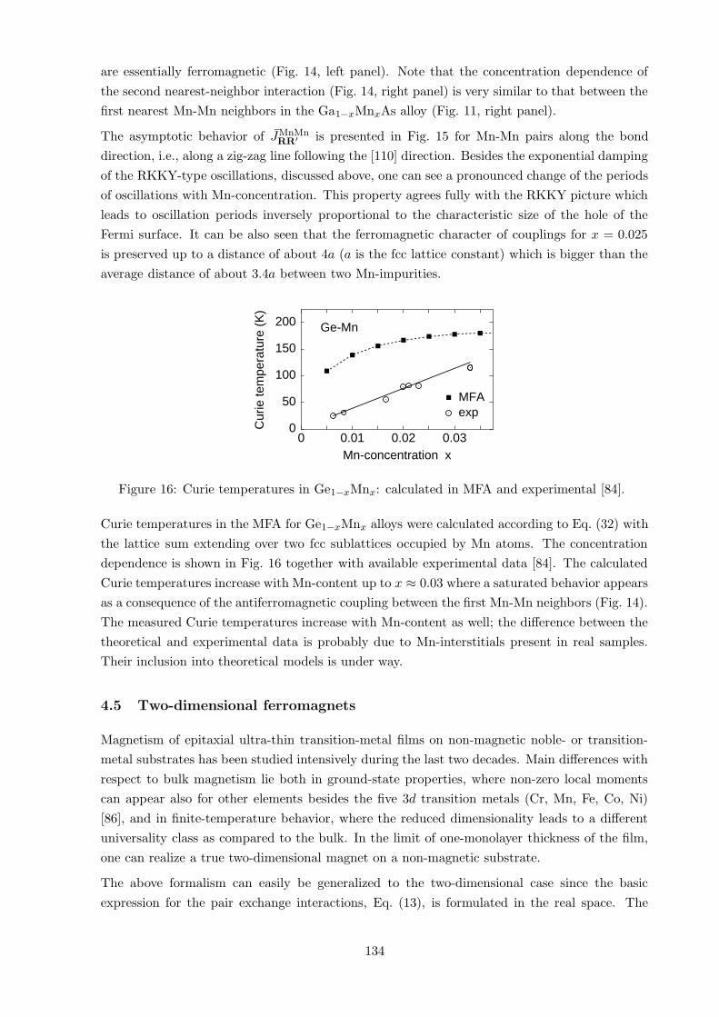
Figure 16: Curie temperatures in Ge1−xMnx: calculated in MFA and experimental [84].

Curie temperatures in the MFA for Ge1−xMnx alloys were calculated according to Eq. (32) with

the lattice sum extending over two fcc sublattices occupied by Mn atoms. The concentration

dependence is shown in Fig. 16 together with available experimental data [84]. The calculated

Curie temperatures increase with Mn-content up to x ≈ 0.03 where a saturated behavior appears

as a consequence of the antiferromagnetic coupling between the first Mn-Mn neighbors (Fig. 14).

The measured Curie temperatures increase with Mn-content as well; the difference between the

theoretical and experimental data is probably due to Mn-interstitials present in real samples.

Their inclusion into theoretical models is under way.

4.5 Two-dimensional ferromagnets

Magnetism of epitaxial ultra-thin transition-metal films on non-magnetic noble- or transition-

metal substrates has been studied intensively during the last two decades. Main differences with

respect to bulk magnetism lie both in ground-state properties, where non-zero local moments

can appear also for other elements besides the five 3d transition metals (Cr, Mn, Fe, Co, Ni)

[86], and in finite-temperature behavior, where the reduced dimensionality leads to a different

universality class as compared to the bulk. In the limit of one-monolayer thickness of the film,

one can realize a true two-dimensional magnet on a non-magnetic substrate.

The above formalism can easily be generalized to the two-dimensional case since the basic

expression for the pair exchange interactions, Eq. (13), is formulated in the real space. The

134

magnetic properties resulting from a two-dimensional EHH can be obtained in a similar way

like in the bulk case, see Eqs. (6, 7, 8, 9), with the reciprocal-space vector q replaced by a

two-dimensional vector q‖ in the surface Brillouin zone (SBZ) and with the real-space sums

restricted to lattice sites R, R′ of the magnetic film. The site-off-diagonal blocks gσRR′(z) of the

Green function in Eq. (13) are determined using the surface Green function technique [35, 36],

while the definition of ∆R(z) remains unchanged. The magnon energies are given by

E(q‖) =4

M

[

J(0‖) − J(q‖)]

+ ∆ , J(q‖) =∑

R

J0R exp(iq‖ · R) , (34)

where ∆ is a magnetic anisotropy energy which is a consequence of relativistic effects (spin-orbit

interaction, magnetostatic dipole-dipole interaction). The Curie temperature in the MFA is

given by Eq. (8) while the RPA leads to an expression

(

kBTRPAC

)−1=

6

M

1

N‖

∑

q‖

1

E(q‖), (35)

where N‖ is the number of q‖-vectors used in the SBZ-average.

-1

0

1

1 2 3 4 5 6 7

(d/a

)2 J (

mR

y)

d/a

Co

Figure 17: Exchange interactions JRR′ multiplied by a prefactor d2 for Co-moments in a Co-

overlayer on an fcc Cu(001) substrate as a function of the distance |R − R′| = d.

The calculated pair exchange interactions JRR′ in a Co-monolayer on an fcc Cu(001) substrate

are shown in Fig. 17. The first nearest-neighbor interaction dominates and the next-neighbor

interactions exhibit an RKKY-like oscillatory behavior with an envelope decaying proportionally

to |R − R′|−2, in contrast to the bulk decay proportional to |R − R′|−3. Note, however, that

the present case is not strictly two-dimensional due to the indirect exchange interactions of two

Co-overlayer atoms via the Cu-substrate, which becomes weakly polarized in the atomic layers

adjacent to the overlayer.

The indirect interaction between the magnetic atoms, which is mediated by the non-magnetic

atoms, has important consequences for magnetic properties of magnetic films placed on a non-

magnetic substrate and covered by a non-magnetic cap-layer of a finite thickness. As reported

in a recent experiment [87], the Curie temperature of fcc(001)-Fe ultrathin films on a Cu(001)

substrate varies in a non-monotonous manner as a function of the Cu cap-layer thickness. Such

a behavior clearly cannot be explained within a localized picture of magnetism.

Motivated by this finding we performed a systematic study of Fe- and Co-monolayers on an fcc

Cu(001) substrate capped by another Cu-layer of varying thickness [13, 15]. Figure 18 presents

the magnon spectra in two limiting cases, namely, for an uncovered Fe-overlayer on Cu(001)

135

0

100

200

300

400

500

Ene

rgy

[meV

]

M X MΓ

Fe

DOS

Figure 18: Magnon dispersion laws (left panel) and corresponding densities of states (right panel)

for an Fe-layer embedded in fcc Cu (full lines) and an Fe-overlayer on fcc Cu(001) (dashed lines).

We have set here ∆ = 0 in Eq. (34).

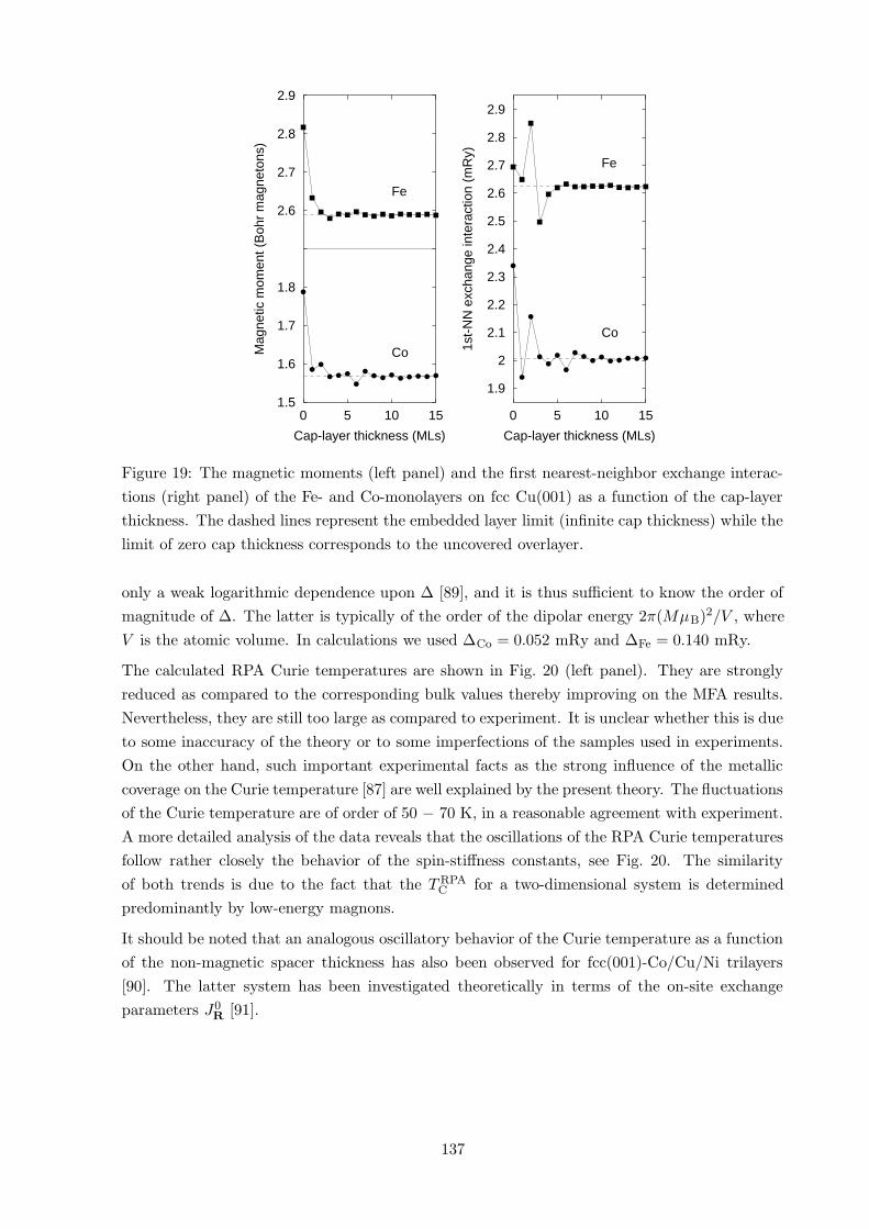
and for an Fe-monolayer embedded in bulk Cu, and figure 19 shows the full dependence of

the magnetic moments and the first nearest-neighbor exchange interactions on the cap-layer

thickness. The magnon spectra and the magnon densities of states exhibit all typical features

of two-dimensional bands with the nearest-neighbor interactions which are here only slightly

modified by non-vanishing interactions in next shells. The magnetic moments drop substantially

on capping while their sensitivity to increasing cap-layer thickness is rather small. On the other

hand, the behavior of the nearest-neighbor exchange interaction is more complicated and it

reflects interference effects in the Cu-cap layer. The oscillations visible in right panel of Fig. 19

are due to quantum-well states in the Cu-cap layer formed between the vacuum and the magnetic

layer which, in turn, influence properties of the magnetic layer. Note that the values of the

nearest-neighbor exchange interaction are significantly enhanced (roughly by a factor 2 or more)

as compared with their bulk counterparts (cf. Fig. 1).

Calculations of the Curie temperatures of the two-dimensional ferromagnets represent a more

difficult task than in the bulk case. The MFA Curie temperatures of the monolayers are typically

of the same order of magnitude as the corresponding bulk temperatures [13] due to the fact

that the reduced coordination is approximately compensated by the increase of the exchange

interactions. This observation is in a strong disagreement with experimental data which yield

the Curie temperatures of the order 150 − 200 K. This failure is due to the fact that the MFA

violates the Mermin-Wagner theorem [88] due to the neglect of collective transverse fluctuations

(spin-waves) and it is thus inappropriate for two-dimensional systems.

Application of the RPA to the Curie temperature of a two-dimensional isotropic EHH, Eq. (35)

with ∆ = 0, yields a vanishing T RPAC in agreement with the Mermin-Wagner theorem. Finite

values of T RPAC require non-zero values of the magnetic anisotropy energy ∆ which is taken here

as an adjustable parameter. This is not a serious problem as the RPA Curie temperature has

136

1.5

1.6

1.7

1.8

2.6

2.7

2.8

2.9

0 5 10 15

Mag

netic

mom

ent (

Boh

r m

agne

tons

)

Cap-layer thickness (MLs)

Fe

Co

1.9

2

2.1

2.2

2.3

2.4

2.5

2.6

2.7

2.8

2.9

0 5 10 15

1st-

NN

exc

hang

e in

tera

ctio

n (m

Ry)

Cap-layer thickness (MLs)

Fe

Co

Figure 19: The magnetic moments (left panel) and the first nearest-neighbor exchange interac-

tions (right panel) of the Fe- and Co-monolayers on fcc Cu(001) as a function of the cap-layer

thickness. The dashed lines represent the embedded layer limit (infinite cap thickness) while the

limit of zero cap thickness corresponds to the uncovered overlayer.

only a weak logarithmic dependence upon ∆ [89], and it is thus sufficient to know the order of

magnitude of ∆. The latter is typically of the order of the dipolar energy 2π(MµB)2/V , where

V is the atomic volume. In calculations we used ∆Co = 0.052 mRy and ∆Fe = 0.140 mRy.

The calculated RPA Curie temperatures are shown in Fig. 20 (left panel). They are strongly

reduced as compared to the corresponding bulk values thereby improving on the MFA results.

Nevertheless, they are still too large as compared to experiment. It is unclear whether this is due

to some inaccuracy of the theory or to some imperfections of the samples used in experiments.

On the other hand, such important experimental facts as the strong influence of the metallic

coverage on the Curie temperature [87] are well explained by the present theory. The fluctuations

of the Curie temperature are of order of 50 − 70 K, in a reasonable agreement with experiment.

A more detailed analysis of the data reveals that the oscillations of the RPA Curie temperatures

follow rather closely the behavior of the spin-stiffness constants, see Fig. 20. The similarity

of both trends is due to the fact that the T RPAC for a two-dimensional system is determined

predominantly by low-energy magnons.

It should be noted that an analogous oscillatory behavior of the Curie temperature as a function

of the non-magnetic spacer thickness has also been observed for fcc(001)-Co/Cu/Ni trilayers

[90]. The latter system has been investigated theoretically in terms of the on-site exchange

parameters J0R [91].

137

200

300

400

500

600

700

0 5 10 15

Cur

ie te

mpe

ratu

re (

K)

Cap-layer thickness (MLs)

Fe

Co

300

400

500

300

400

500

600

0 5 10 15

Stif

fnes

s co

nsta

nt (

meV

A )2

o .

Cap-layer thickness (MLs)

Fe

Co

Figure 20: The Curie temperatures (left panel) and the spin-stiffness constants (right panel)

of the Fe- and Co-monolayers on fcc Cu(001) as a function of the cap-layer thickness. The

dashed lines represent the embedded layer limit (infinite cap thickness) while the limit of zero

cap thickness corresponds to the uncovered overlayer case.

4.6 Surfaces of ferromagnets

Reduced coordination at surfaces of transition-metal ferromagnets leads to an enhancement

of surface magnetic moments over their bulk values [86]. For the ferromagnetic hcp Gd, an

enhancement of its Curie temperature at (0001) surface over the bulk value was observed [92].

Theoretical explanation of the latter fact was provided by total-energy calculations using an

LSDA+U approach [93]. An important role was ascribed to a small inward relaxation of the

top surface layer. However, more recent works have thrown serious doubts on these conclusions,

both on side of experiment [94] and theory [63].

We have recently performed calculations for low-index surfaces of bcc Fe, hcp Co, and hcp Gd [19]

focused on layer-resolved local quantities like the magnetic moments and the on-site exchange

parameters J0R, Eq. (17). Note, however, that for inhomogeneous systems like surfaces, a direct

relation between the Curie temperatures and the on-site exchange parameters J 0R cannot be

given. Hence, the latter quantities reflect merely the strength of the exchange interaction and

its spatial variations in layered systems [91].

Figure 21 presents the results for Fe- and Co-surfaces. It is seen that the well-known surface

enhancement of the moments is accompanied by a more complicated layer-dependence of the

on-site exchange parameters exhibiting a minimum in the top surface layer and a maximum

in the first subsurface layer. A qualitative explanation follows from Eqs. (13, 17) which show

that J0R reflects the exchange splitting on the R-th site as well as the splittings and number

of its neighbors. Hence, the reduction of J 0R in the top surface layer is due to the reduced

coordination, whereas the maximum in the first subsurface position is due to the full (bulk-like)

138

1.5

2.0

2.5

3.0

0 1 2 3 4 5 6

Mag

netic

mom

ent (

µ B)

Layer

Fe(001)

Fe(110)

Co(0001)

6

10

14

18

0 1 2 3 4 5 6

On-

site

exc

hang

e pa

ram

eter

(m

Ry)

Layer

Co(0001)

Fe(001)

Fe(110)

Figure 21: Layer-resolved magnetic moments (left panel) and on-site exchange parameters J 0R

(right panel) at surfaces of bcc Fe and hcp Co. The layer numbering starts from the top surface

layer, denoted by 0.

coordination of these sites and the enhanced surface local moments, see Fig. 21. Note that the

layer-dependence of the on-site exchange parameters and its explanation are analogous to the

case of hyperfine magnetic fields at the nuclei of iron atoms [35, 95].

The Gd(0001) surface was treated in the ‘open-core’ approach mentioned in Section 4.2. Two

models of the surface structure were used: with lattice sites occupying the ideal truncated bulk

positions (unrelaxed structure) and with a 3% contraction of the interlayer separation between

the two topmost atomic layers (inward relaxation). The magnitude of the contraction was set

according to LEED measurements [96] and previous full-potential calculations [63]. The layer-

resolved quantities are presented in Figure 22. The layer-resolved magnetic moments exhibit

a small surface enhancement followed by Friedel-like oscillations around the bulk value. These

oscillations can be resolved also in the layer-dependence of the on-site exchange parameters J 0R

which, however, start with reduced values in the top surface layer due to the reduced coordina-

tion, as discussed for Fe- and Co-surfaces. The maximum of the on-site exchange parameters

is found in the second subsurface layer, in contrast to the transition-metal surfaces, which can

be explained by the reduced Gd-moments in the first subsurface layer. The surface relaxation

does not modify investigated layer-dependences substantially: it leads to a small reduction of

the local moments and the on-site exchange parameters in the first two top surface layers and a

tiny enhancement in the second subsurface layer as compared to the ideal surface.

One can conclude that the surface enhancement of the local magnetic moments of the three

ferromagnetic metals is not accompanied by an analogous trend of on-site exchange parameters

which might be an indication of a surface-induced enhancement of Curie temperatures. However,

a calculation of the pair exchange interactions and an improved treatment of the EHH beyond

the MFA remain important tasks for future.

139

7.4

7.5

7.6

7.7

7.8

7.9

8.0

0 1 2 3 4 5 6

Mag

netic

mom

ent (

µ B)

Layer

Gd(0001)

ideal

relaxed

2.0

3.0

4.0

0 1 2 3 4 5 6

On-

site

exc

hang

e pa

ram

eter

(m

Ry)

Layer

Gd(0001)

ideal

relaxed

Figure 22: Layer-resolved magnetic moments (left panel) and on-site exchange parameters J 0R

(right panel) at the (0001) surface of hcp Gd as calculated with the lattice sites in the ideal

truncated bulk positions and with the top surface layer relaxed towards the bulk. The layer

numbering starts from the top surface layer, denoted by 0.

5 Discussion and outlook

Exchange interactions and related quantities can be extracted from selfconsistent electronic

structure calculations in a number of different ways; each of them has its own advantages

and disadvantages. The simplest approach lies in obtaining the exchange interactions from

total-energy differences calculated directly for various (usually collinear) spin configurations

[63, 97, 98]. The usefulness of such schemes is, however, rather limited mainly due to a finite

number of configurations used for the mapping.

The real-space method presented here allows to get a set of pair interactions even for very distant

atoms only from a single selfconsistent calculation. It has therefore been used independently

in a number of papers for very different systems [51, 99, 100, 101]. A widely used alternative

approach, the so-called frozen-magnon approach, relies on constrained DFT calculations for true

spin spirals and subsequent derivation of the coupling constants from the total energies of the

spirals [27, 43, 44]. The frozen-magnon approach can be implemented with the magnetic force

theorem [83] or can be formulated in terms of torques instead of total energies [102]. The real-

space and frozen-magnon approaches are formally equivalent to each other. The quantities that

are directly calculated (the pair exchange interactions JRR′ in the former case, the magnon

energies E(q)’s in the latter) are related to each other by a lattice Fourier transformation,

Eq. (6). For this reason, their advantages and disadvantages refer mainly to their computational

efficiency. For calculations of spin-wave dispersion curves (for a moderate number of q-points)

and of the spin-wave stiffness D, the frozen-magnon approach is superior, for it does not require

to perform the Fourier transformation and the delicate analysis explained in Section 3.3. The

real-space approach seems to be more efficient for calculations of the Curie temperature, where

the MFA estimation can be obtained from Eq. (8) and the sum rule (17), i.e., from a single

real-space calculation, whereas a BZ-average of the magnon energies E(q) is required in the

140

frozen-magnon approach. The real-space technique is better also when a fine scan over the full

BZ is needed like, e.g., in RPA calculations of the Curie temperature, Eq. (9), or in searching

for instabilities of the ferromagnetic state (see Section 4.2), since the set of calculated JRR′ for

typically 200 shells provides a fast and accurate parametrization of J(q), which considerably

reduces the computational effort.

The central idea of mapping the infinitesimal changes of single-particle energies onto an effec-

tive classical Hamiltonian for localized spins has been used also for a quantitative description of

effects beyond the bilinear isotropic exchange interaction in Eq. (2). Higher terms in expansion

of the single-particle energies with respect to rotation angles give rise to biquadratic exchange

interaction, important especially in metallic multilayers [103]. Inclusion of relativistic effects,

leading to anisotropic exchange interaction and Dzialoshinskii-Moriya interaction, has been dis-

cussed for bulk systems [52, 104] and thin films [105]. In both cases, the gap in the spin-wave

spectrum for zero wavevector can be calculated with accuracy better than used in Section 4.5

for quantity ∆ in Eq. (34). The magnetic force theorem and expressions for effective interaction

parameters have recently been formulated also for highly correlated systems treated beyond the

LSDA [106].

It should be noted, however, that certain aspects of finite-temperature itinerant magnetism

cannot be reproduced by effective Hamiltonians with one unit vector per atomic site only. An

ab initio study based on a model Hamiltonian with bilinear, biquadratic and bicubic terms

depending on the magnitude of local magnetic moments was formulated in Ref. [107]. The

parametrization of the model was obtained from selfconsistent calculations for a number of spin-

spiral states. The calculated Curie temperature of bcc Fe agrees well with experiment while the

Curie temperatures of fcc Co and fcc Ni were underestimated by about 20 − 25%.

Another ab initio approach based on effective Hamiltonians acting on more than one magnetic

vector per atom was worked out in Refs. [43, 62]. It is based on a well-defined spatial separability

of the sp- and d-components of the spin density in late 3d transition metals leading thus to

two spin vectors per atom. Results of this approach for the magnon spectrum of fcc Ni seem

to describe qualitatively well finer details in the experimental data around 100 − 150 meV

(sometimes denoted as an ‘optical’ magnon), which are manifestation of non-adiabatic effects

[43]. In the case of heavy RE-metals (Gd through Tm), three moment vectors per site were

considered: the conduction electron (spd) spin moment vector and the 4f electron spin and

orbital moment vectors. The effective Hamiltonian in the latter case contains also intrasite spin-

orbit coupling interaction and crystal-field terms. A first-principles approach to crystal-field

parameters in RE-based systems can be found in Refs. [60, 108].

As mentioned in Section 2, the pair exchange interactions according to Eq. (5) do not contain

contributions from constraining magnetic fields which appear as Lagrange multipliers in the

constrained DFT. Their effect has been recently addressed in Refs. [24, 26]; it leads to a mod-

ification of the pair exchange interactions and related quantities. The changes of the moment

directions δuR and the constraining fields B⊥R satisfy linear relations [24]

MR δuR =∑

R′

(

KRR′ δuR′ + χRR′ B⊥R′

)

, (36)

where MR denotes the magnitude of R-th local moment in units of µB and where the exchange-

141

correlation response function KRR′ and the bare transverse susceptibility χRR′ are given by

KRR′ =2

πIm

∫ EF

−∞dE

∫

ΩR

dr

∫

ΩR′

dr′ G↑(r, r′; E + i0) Bxc(r′) G↓(r′, r; E + i0) ,

χRR′ =2

πIm

∫ EF

−∞dE

∫

ΩR

dr

∫

ΩR′

dr′ G↑(r, r′; E + i0) G↓(r′, r; E + i0) . (37)

As a consequence of non-zero constraining fields, the exchange parameters JRR′ get renormalized

values given explicitly by [24]

J renRR′ = JRR′ − 1

2

(M − KT ) X−1 (M − K)

RR′, (38)

where M,K,X denote, respectively, matrices with elements MR δRR′ , KRR′ , χRR′ , and where

KT denotes the transpose of K. The evaluation of Eq. (38) for real systems remains yet to be

performed.

Some physical insight into the nature of this renormalization can be obtained for Bravais lattices

assuming a sufficiently rigid magnetization within an atomic cell [24]. With a definition of an

average exchange splitting on site R,

∆R =2

MR

∫

ΩR

dr m(r) Bxc(r) , (39)

where m(r) is the spin density, it can be shown that the renormalization of the pair interactions,

Eq. (38), leads to a simple renormalization of the magnon energies E(q) which is significant

for high-energy magnons E(q) > ∆ (where ∆ = ∆R for a Bravais lattice). In particular, the

spin-wave stiffness constant D does not undergo any renormalization. The Curie temperature

evaluated in the RPA becomes renormalized according to a formula

(

kBTRPA,renC

)−1=(

kBTRPAC

)−1− 6

M∆, (40)

which means that the renormalized Curie temperatures are enhanced as compared to the un-

renormalized ones. The values for the bulk cubic 3d ferromagnets are summarized in Table 3. It

can be seen that the renormalization of exchange parameters improves considerably the agree-

ment between theory and experiment for Fe and Ni, in contrast to Co, where the unrenormalized

Curie temperature is closer to experiment than the renormalized one. A quantitative analysis

for bulk Gd shows that the effect of constraining fields is completely negligible [26].

Table 3: Curie temperature calculated within the RPA by using the bare (T RPAC ) and renormal-

ized (T RPA,renC ) exchange interactions and their comparison with experimental values (TC,exp).

Metal T RPAC [K] TRPA,ren

C [K] TC,exp[K]

Fe bcc 950 1057 1044 − 1045

Co fcc 1311 1771 1388 − 1398

Ni fcc 350 634 624 − 631

As is well known, the exact magnon dispersion law is obtained from poles of the dynamical

transverse susceptibility while the effective exchange interactions are closely related to the static

142

transverse susceptibility [26]. Susceptibility calculations within the DFT are, however, quite

involved even for systems with perfect three-dimensional translational symmetry [109, 110],

which calls for additional approximations. The calculations can be simplified using again the

adiabatic approximation and the ASA as done in Ref. [102]. The spin-wave spectrum of bcc Fe

calculated from the susceptibility agrees very well with that from a frozen-magnon approach,

whereas differences between the two approaches are found in results for fcc Co and fcc Ni [102].

However, for a correct reproduction of the ‘optical’ magnon branch of fcc Ni (including the

lifetime effects), full susceptibility calculations [110] are inevitable.

Susceptibility calculations have been employed in another successful approach to finite-tempe-

rature magnetism, based on the DLM state with local magnetic moments pointing to random

directions [21, 111]. In contrast to the previous techniques starting from the magnetic ground

state and its excitations, the DLM theory is focused on the paramagnetic state whereby no

particular form of an effective spin Hamiltonian has to be assumed. The transition temperature

is derived from divergence of the susceptibility of the DLM state which is related to a direct

correlation function. An efficient evaluation of the latter quantity represents the most difficult

part of computations. This mean-field technique has been applied to bulk bcc Fe and fcc Ni [54];

an especially good agreement between the calculated and experimental Curie temperatures has

been achieved by including effects of correlations in terms of Onsager cavity fields. Applications

to thin transition-metal films have been restricted to the mean-field level [112, 113]; the results

for the Curie temperatures reproduce a number of experimentally observed trends with respect

to the thickness of magnetic films and of non-magnetic capping layers. In the case of Fe and

Co monolayers on a Cu(001) substrate, however, the theory predicts unrealistically high Curie

temperatures, in full agreement with the MFA values from the EHH, see Section 4.5 and Ref. [13].

The most important feature of the described ab initio approach to exchange interactions lies in

its real-space formulation, which opens a way to study long-range interactions encountered in

itinerant magnets including systems without three-dimensional translational invariance (random

alloys, low-dimensional magnets). The inherent limitation to cases with large local magnetic

moments makes the approach especially suitable for applications to systems like transition-metal

surfaces and thin films, diluted magnetic semiconductors, rare-earth metals and compounds, etc.

Acknowledgements

We are grateful to L. Bergqvist, G. Bihlmayer, S. Blugel, G. Bouzerar, M. Divis, P. Franek, F.

Maca, M. Pajda, J. Rusz and P. Weinberger for collaboration at various stages of the project,

and to P. Dederichs, B. Gyorffy, P. Levy, A. Liechtenstein, A. Shick, L. Szunyogh and L. Udvardi

for helpful discussions.

We acknowledge the financial support provided by the Grant Agency of the Czech Republic (No.

106/02/0943), the Academy of Sciences of the Czech Republic (No. A1010203 and Z2041904), the

Ministry of Education of the Czech Republic (MSM113200002), the Center for Computational

Materials Science in Vienna (GZ 45.504), and the RT Network ‘Computational Magnetoelec-

tronics’ (Contract HPRN-CT-2000-00143) of the European Commission.

143

References

[1] P. Hohenberg and W. Kohn. Phys. Rev., 136:B864, 1964.

[2] W. Kohn and L. J. Sham. Phys. Rev., 140:A1133, 1965.

[3] U. von Barth and L. Hedin. J. Phys. C, 5:1629, 1972.

[4] J. B. Staunton. Rep. Progr. Phys., 57:1289, 1994.

[5] J. Kubler. Theory of Itinerant Electron Magnetism. Clarendon Press, Oxford, 2000.

[6] K. Baberschke, M. Donath, and W. Nolting, editors. Band-Ferromagnetism, volume 580 of Lecture

Notes in Physics. Springer, Berlin, 2001.

[7] P. Mohn. Magnetism in the Solid State. Springer, Berlin, 2003.

[8] E. Runge and E. K. U. Gross. Phys. Rev. Lett., 52:997, 1984.

[9] N. D. Mermin. Phys. Rev., 137:A1441, 1965.

[10] A. I. Liechtenstein, M. I. Katsnelson, and V. A. Gubanov. J. Phys. F, 14:L125, 1984.

[11] A. I. Liechtenstein, M. I. Katsnelson, V. P. Antropov, and V. A. Gubanov. J. Magn. Magn. Mater.,

67:65, 1987.

[12] V. P. Antropov, B. N. Harmon, and A. N. Smirnov. J. Magn. Magn. Mater., 200:148, 1999.

[13] M. Pajda, J. Kudrnovsky, I. Turek, V. Drchal, and P. Bruno. Phys. Rev. Lett., 85:5424, 2000.

[14] M. Pajda, J. Kudrnovsky, I. Turek, V. Drchal, and P. Bruno. Phys. Rev. B, 64:174402, 2001.

[15] P. Bruno, J. Kudrnovsky, M. Pajda, V. Drchal, and I. Turek. J. Magn. Magn. Mater., 240:346,

2002.

[16] J. Kudrnovsky, I. Turek, V. Drchal, F. Maca, J. Masek, P. Weinberger, and P. Bruno. J. Super-

conductivity, 16:119, 2003.

[17] I. Turek, J. Kudrnovsky, G. Bihlmayer, and S. Blugel. J. Phys.: Condens. Matter, 15:2771, 2003.

[18] I. Turek, J. Kudrnovsky, V. Drchal, P. Bruno, and S. Blugel. Physica Status Solidi B, 236:318,

2003.

[19] I. Turek, G. Bihlmayer, S. Blugel, and P. Weinberger. Czech. J. Phys., 53:81, 2003.

[20] G. Bouzerar, J. Kudrnovsky, L. Bergqvist, and P. Bruno. Phys. Rev. B, 68:081203, 2003.

[21] B. L. Gyorffy, A. J. Pindor, J. Staunton, G. M. Stocks, and H. Winter. J. Phys. F, 15:1337, 1985.

[22] P. H. Dederichs, S. Blugel, R. Zeller, and H. Akai. Phys. Rev. Lett., 53:2512, 1984.

[23] L. M. Sandratskii. J. Phys.: Condens. Matter, 3:8565, 1991.

[24] P. Bruno. Phys. Rev. Lett., 90:087205, 2003.

[25] A. Oswald, R. Zeller, P. J. Braspenning, and P. H. Dederichs. J. Phys. F, 15:193, 1985.

[26] V. P. Antropov. J. Magn. Magn. Mater., 262:L192, 2003.

[27] S. V. Halilov, H. Eschrig, A. Y. Perlov, and P. M. Oppeneer. Phys. Rev. B, 58:293, 1998.

[28] V. P. Antropov, M. I. Katsnelson, M. van Schilfgaarde, and B. N. Harmon. Phys. Rev. Lett., 75:729,

1995.

[29] V. P. Antropov, M. I. Katsnelson, B. N. Harmon, M. van Schilfgaarde, and D. Kusnezov. Phys.

Rev. B, 54:1019, 1996.

144

[30] Q. Niu and L. Kleinman. Phys. Rev. Lett., 80:2205, 1998.

[31] Q. Niu, X. Wang, L. Kleinman, W.-M. Liu, D. M. C. Nicholson, and G. M. Stocks. Phys. Rev.

Lett., 83:207, 1999.

[32] S. V. Tyablikov. Methods of Quantum Theory of Magnetism. Plenum Press, New York, 1967.

[33] C. S. Wang, R. E. Prange, and V. Korenman. Phys. Rev. B, 25:5766, 1982.

[34] O. K. Andersen and O. Jepsen. Phys. Rev. Lett., 53:2571, 1984.

[35] I. Turek, V. Drchal, J. Kudrnovsky, M. Sob, and P. Weinberger. Electronic Structure of Disordered

Alloys, Surfaces and Interfaces. Kluwer, Boston, 1997.

[36] I. Turek, J. Kudrnovsky, and V. Drchal. In H. Dreysse, editor, Electronic Structure and Physical

Properties of Solids, volume 535 of Lecture Notes in Physics, page 349. Springer, Berlin, 2000.

[37] S. H. Vosko, L. Wilk, and M. Nusair. Can. J. Phys., 58:1200, 1980.

[38] P. Weinberger. Electron Scattering Theory for Ordered and Disordered Matter. Clarendon Press,

Oxford, 1990.

[39] A. Gonis. Green Functions for Ordered and Disordered Systems. North-Holland, Amsterdam, 1992.

[40] O. Gunnarsson, O. Jepsen, and O. K. Andersen. Phys. Rev. B, 27:7144, 1983.

[41] P. Bruno. Phys. Rev. B, 52:411, 1995.

[42] K. C. Hass, B. Velicky, and H. Ehrenreich. Phys. Rev. B, 29:3697, 1984.

[43] S. Halilov. In D. J. Singh and D. A. Papaconstantopoulos, editors, Electronic Structure and Mag-

netism of Complex Materials, volume 54 of Springer Series in Materials Science, chapter 1, page 1.

Springer, Berlin, 2003.

[44] M. van Schilfgaarde and V. P. Antropov. J. Appl. Phys., 85:4827, 1999.

[45] C. K. Loong, J. M. Carpenter, J. W. Lynn, R. A. Robinson, and H. A. Mook. J. Appl. Phys.,

55:1895, 1984.

[46] J. W. Lynn. Phys. Rev. B, 11:2624, 1975.

[47] H. A. Mook and D. McK. Paul. Phys. Rev. Lett., 54:227, 1985.

[48] G. Shirane, V. J. Minkiewicz, and R. Nathans. J. Appl. Phys., 39:383, 1968.

[49] H. A. Mook, J. W. Lynn, and M. R. Nicklow. Phys. Rev. Lett., 30:556, 1973.

[50] R. Pauthenet. J. Appl. Phys., 53:2029 and 8187, 1982.

[51] D. Spisak and J. Hafner. J. Magn. Magn. Mater., 168:257, 1997.

[52] V. P. Antropov, M. I. Katsnelson, and A. I. Liechtenstein. Physica B, 237-238:336, 1997.

[53] R. H. Brown, D. M. C. Nicholson, X. Wang, and T. C. Schulthess. J. Appl. Phys., 85:4830, 1999.

[54] J. B. Staunton and B. L. Gyorffy. Phys. Rev. Lett., 69:371, 1992.

[55] M. Heinemann and W. M. Temmerman. Phys. Rev. B, 49:4348, 1994.

[56] J. Jensen and A. R. Mackintosh. Rare Earth Magnetism. Clarendon, Oxford, 1991.

[57] B. N. Harmon, V. P. Antropov, A. I. Liechtenstein, I. V. Solovyev, and V. I. Anisimov. J. Phys.

Chem. Solids, 56:1521, 1995.

[58] A. B. Shick, A. I. Liechtenstein, and W. E. Pickett. Phys. Rev. B, 60:10763, 1999.

[59] P. Strange, A. Svane, W. M. Temmerman, Z. Szotek, and H. Winter. Nature, 399:756, 1999.

145

[60] M. Richter. J. Phys. D, 31:1017, 1998.

[61] M. S. S. Brooks, L. Nordstrom, and B. Johansson. J. Phys.: Condens. Matter, 3:2357, 1991.

[62] A. Y. Perlov, S. V. Halilov, and H. Eschrig. Phys. Rev. B, 61:4070, 2000.

[63] P. Kurz, G. Bihlmayer, and S. Blugel. J. Phys.: Condens. Matter, 14:6353, 2002.

[64] P. A. Lindgard. Phys. Rev. B, 17:2348, 1978.

[65] N. G. Nereson, C. E. Olsen, and G. P. Arnold. Phys. Rev., 135:A176, 1964.

[66] A. H. Millhouse and K. A. McEwen. Solid State Commun., 13:339, 1973.

[67] P. Franek. Master’s thesis, Charles University, Prague, 2003.

[68] M. S. S. Brooks and B. Johansson. In K. H. J. Buschow, editor, Handbook of Magnetic Materials,

volume 7, chapter 3, page 139. North-Holland, Amsterdam, 1993.

[69] I. Turek, J. Kudrnovsky, M. Divis, P. Franek, G. Bihlmayer, and S. Blugel. Phys. Rev. B, (submit-

ted).

[70] J. Kudrnovsky and V. Drchal. Phys. Rev. B, 41:7515, 1990.

[71] P. Bruno, J. Kudrnovsky, V. Drchal, and I. Turek. Phys. Rev. Lett., 76:4254, 1996.

[72] J. Kudrnovsky, V. Drchal, I. Turek, P. Bruno, P. Dederichs, and P. Weinberger. In H. Dreysse,

editor, Electronic Structure and Physical Properties of Solids, volume 535 of Lecture Notes in

Physics, page 313. Springer, Berlin, 2000.

[73] P. M. Levy, S. Maekawa, and P. Bruno. Phys. Rev. B, 58:5588, 1998.

[74] S. D. Drell and L. Verlet. Phys. Rev., 99:849, 1955.

[75] G. Bouzerar and P. Bruno. Phys. Rev. B, 66:014410, 2002.

[76] S. Ghosh, P. L. Leath, and M. H. Cohen. Phys. Rev. B, 66:214206, 2002.

[77] H. Akai. Phys. Rev. Lett., 81:3002, 1998.

[78] H. Ohno. J. Magn. Magn. Mater., 200:110, 1999.

[79] K. W. Edmonds et al. Appl. Phys. Lett., 81:4991, 2002.

[80] F. Maca and J. Masek. Phys. Rev. B, 65:235209, 2002.

[81] P. A. Korzhavyi et al. Phys. Rev. Lett., 88:187202, 2002.

[82] K. Sato, P. H. Dederichs, and H. Katayama-Yoshida. Europhys. Lett., 61:403, 2003.

[83] L. M. Sandratskii and P. Bruno. Phys. Rev. B, 66:134435, 2002.

[84] Y. D. Park et al. Science, 295:651, 2002.

[85] B. T. Jonker et al. cond-mat/0302231.

[86] M. Weinert and S. Blugel. In L. H. Bennett and R. E. Watson, editors, Magnetic Multilayers,

page 51. World Scientific, Singapore, 1994.

[87] R. Vollmer, S. van Dijken, M. Schleberger, and J. Kirschner. Phys. Rev. B, 61:1303, 2000.

[88] N. D. Mermin and H. Wagner. Phys. Rev. Lett., 17:1133, 1966.

[89] P. Bruno. Mater. Res. Soc. Symp. Proc., 321:299, 1992.

[90] A. Ney, F. Wilhelm, M. Farle, P. Poulopoulos, P. Srivastava, and K. Baberschke. Phys. Rev. B,

59:R3938, 1999.

146

[91] E. I. Isaev, L. V. Pourovskii, A. M. N. Niklasson, Yu. Kh. Vekilov, B. Johansson, and I. A.

Abrikosov. Phys. Rev. B, 65:024435, 2001.

[92] E. D. Tober et al. Phys. Rev. Lett., 81:2360, 1998.

[93] A. B. Shick, W. E. Pickett, and C. S. Fadley. Phys. Rev. B, 61:R9213, 2000.

[94] C. S. Arnold and D. P. Pappas. Phys. Rev. Lett., 85:5202, 2000.

[95] S. Blugel. In Magnetismus von Festkorpern und Grenzflachen. Forschungszentrum Julich, 1993.

[96] J. Giergiel, A. W. Pang, H. Hopster, X. Guo, S. Y. Tong, and D. Weller. Phys. Rev. B, 51:10201,

1995.

[97] D. Spisak and J. Hafner. Phys. Rev. B, 65:235405, 2002.

[98] D. Kodderitzsch, W. Hergert, W. M. Temmerman, Z. Szotek, A. Ernst, and H. Winter. Phys. Rev.

B, 66:064434, 2002.

[99] R. F. Sabiryanov, S. K. Bose, and O. N. Mryasov. Phys. Rev. B, 51:8958, 1995.

[100] S. Frota-Pessoa, R. B. Muniz, and J. Kudrnovsky. Phys. Rev. B, 62:5293, 2000.

[101] L. Szunyogh and L. Udvardi. J. Magn. Magn. Mater., 198-199:537, 1999.

[102] O. Grotheer, C. Ederer, and M. Fahnle. Phys. Rev. B, 63:100401(R), 2001.

[103] O. N. Mryasov, A. J. Freeman, and A. I. Liechtenstein. J. Appl. Phys., 79:4805, 1996.

[104] V. P. Antropov and A. I. Liechtenstein. Mater. Res. Soc. Symp. Proc., 253:325, 1992.

[105] L. Udvardi, L. Szunyogh, K. Palotas, and P. Weinberger. Phys. Rev. B, 68:1044XX, 2003.

[106] M. I. Katsnelson and A. I. Lichtenstein. Phys. Rev. B, 61:8906, 2000.

[107] N. M. Rosengaard and B. Johansson. Phys. Rev. B, 55:14975, 1997.

[108] P. Novak and J. Kuriplach. Phys. Rev. B, 50:2085, 1994.

[109] J. Callaway, A. K. Chatterjee, S. P. Singhal, and A. Ziegler. Phys. Rev. B, 28:3818, 1983.

[110] S. Y. Savrasov. Phys. Rev. Lett., 81:2570, 1998.

[111] J. B. Staunton, S. S. A. Razee, L. Szunyogh, and B. L. Gyorffy. Physica B, 318:316, 2002.

[112] S. S. A. Razee, J. B. Staunton, L. Szunyogh, and B. L. Gyorffy. Phys. Rev. B, 66:094415, 2002.

[113] S. S. A. Razee, J. B. Staunton, L. Szunyogh, and B. L. Gyorffy. Phys. Rev. Lett., 88:147201, 2002.

147