CEPA Center for Economic Policy Analysis

Exchange rate indeterminacy in portfolio balance, Mundell-Fleming, and uncovered interest rate parity models

Lance Taylor (CEPA)

CEPA Working Paper 2000-21

April 2002

Center for Economic Policy Analysis New School University

80 Fifth Avenue, Fifth Floor, New York, NY 10011-8002 Tel. 212.229.5901 ! Fax 212.229.5903

www.newschool.edu/cepa

1

April 2002

Exchange rate indeterminacy in portfolio balance, Mundell-Fleming, and

uncovered interest rate parity models

Lance Taylor*

With full stock/flow accounting respected, the two-country open economy portfolio balance model has just two independent equations for asset market clearing. It can determine home and foreign interest rates but not the exchange rate. If asset market equilibria vary smoothly over time, the balance of payments equation in the Mundell-Fleming model is not independent and cannot set the exchange rate either. The familiar fixed reserves/ "floating rate" vs. endogenous reserves/"fixed rate" dichotomy does not exist, and "fundamentals-based" econometric models of the exchange rate are bound to fail. An alternative is a two-country IS/LM model with exchange rate dynamics added. Its dynamic properties under uncovered interest rate parity are briefly explored. Key words: Exchange rate, Mundell-Fleming model JEL classifications: F32, F41

For three decades, a central doctrine of open economy macroeconomics has been that the

portfolio balance and Mundell-Fleming (or IS/LM/BP) models - the workhorses of international

finance for policy and teaching purposes - both contain three independent equations that

determine three variables: the home and foreign interest rates and the spot exchange rate.

The gist of this paper is that received wisdom is incorrect. If economic actors satisfy

standard balance sheet and portfolio allocation restrictions, then setting the exchange rate is

beyond the models' reach. The key reason why is that in the short run the home and foreign

economies' nominal net foreign asset (or NFA) holdings are constant. Not only are one country's

external assets the other's liabilities, but at a given exchange rate their net positions can only

____________________________

Address for correspondence: Lance Taylor, CEPA, 80 Fifth Avenue, 5th Floor, New York NY 10011, USA; e-mail taylorl@newschool.edu * Center for Economic Policy Analysis, New School University. Thanks to Wynne Godley for starting me down this track and suggesting the accounting framework, and to Robert Blecker, Serguei Braguinsky, John Eatwell, Duncan Foley, Will Milberg, Jorn Rattso, Jaime Ros, Peter Skott, and careful referees for directions and encouragement along the way. Support from the Ford and John D. and Catherine T. MacArthur Foundations is gratefully acknowledged.

2

change over time via current account surpluses or deficits. In temporary equilibrium, each

country's NFA constraint forces its money market to clear when its bond market is satisfied and

vice-versa.

The arguments supporting these findings proceed in the Keynesian spirit of the models

concerned. We begin in section 1 with an analysis of stock and flow accounts in a two-country

macroeconomic system. Portfolio balance, Mundell-Fleming, and uncovered interest rate parity

(UIP) exchange rate theories are quickly sketched in section 2. The inability of the portfolio

balance model to set the exchange rate is demonstrated in section 3. Section 4 does the same

for Mundell-Fleming. The independent temporary equilibrium conditions that do exist boil down to

linked IS/LM models for the two countries, with activity levels and interest rates (X and *X and i

and *i respectively) as the endogenous variables. Comparative static exercises become of

interest, taking the spot exchange rate ( e ), its expected change over time (ε ), and other

variables as pre-determined. Examples for a "small" home country are presented in section 5.

Section 6 sketches dynamic extensions under the assumption that UIP applies, and a few

additional considerations appear in section 7.

Before jumping into the details, three methodological observations are worth adding.

First, although no one seems to have noted it in the standard models, the irrelevance of the

exchange rate to temporary equilibrium in open economy asset markets has been pointed out in

other contexts, e.g. in a two-country growth model by Foley and Sidrauski (1971), an overlapping

generations model by Kareken and Wallace (1981), and a computable general equilibrium model

by Rosensweig and Taylor (1990).

Second, intertemporal optimization as surveyed by Obstfeld and Rogoff (1995) could be

added to the analysis without altering the tenor of the results. In temporary equilibrium,

intertemporal models incorporate portfolio balances and a real side macro model. Over time, they

use Euler differential equations to determine the exchange rate via UIP and consumption levels

via optimal saving rules a la Ramsey (1928). The Euler equations determine changes in

consumption levels and the exchange rate by intertemporal arbitrage. They are not directly

relevant to the discussion of temporary equilibrium in sections 3-5, which focuses on levels of

3

stocks and flows. In section 6, it is argued that the traditional interpretation of the portfolio balance

model, if correct, would be inconsistent with the intertemporal arbitrage underlying UIP.

Comments about Ramsey rules appear in section 7.

Finally, the results here help explain why an enormous empirical literature finds that

"fundamentals-based" models of the exchange rate have negligible predictive power. If the

standard models cannot determine the spot rate, then econometric tests based upon them will

almost certainly fail.

1. Accounting conundrums

Often the best way to attack a problem in economics is to make sure your accounting is

right. Tables 1 and 2 attempt this task for international trade and financial relations. It is

unfortunately true that full accounting in models containing real and financial sectors requires a

wagonload of symbols. The details in both tables are needed to demonstrate the results that

follow. They follow broadly from a scheme proposed by Godley (1996).

Table 1 sets out the home and foreign countries' flow accounts in the form of a

spreadsheet or social accounting matrix (SAM). Table 2 presents the corresponding balance

sheets. Since the emphasis is on external transactions, economic actors in each country are

aggregated into just three groups - a private sector comprising households and non-financial

business, government, and the banking system which consolidates commercial and central

banks. Variables referring to the home and foreign private sectors are labeled with subscripts h

and f respectively. The foreign country's stocks and flows are denoted by asterisks in both tables.

Tables 1 and 2 here

As shown in Table 2, the primary assets underlying the flow accounts in the SAM are

capital stocks valued at their asset prices (qPK and *** KPq where q and *q are "valuation ratios"

or levels of "Tobin's q") and outstanding short-term bonds or T-bills issued by the two

governments (T and *T , with interest rates i and *i respectively). Both banking systems carry a

subscript b, but they are distinguished by their asset portfolios. The home system's assets are

4

home bonds bT and foreign bonds as reserves with a value *eR ; the foreign system holds

foreign bonds *bT and home bonds as reserves with a local value eR / . The banks have zero net

worth and their liabilities are the money supplies M and *M respectively. In their portfolios, the

private sectors hold the relevant capital stock qPK or *** KPq , both flavors of bonds, and the

local form of money M or *M .1

In the SAM, the two main accounting conventions are that corresponding row and column

totals are equal, and that in each country the entries in each row are valued at the same price.

Accounts for the home country appear to the left, and for the foreign to the right. Cross-border

flows are mediated by "Exchange conversions" between the two sides (the conversions also

involve a sign change because an inflow to one country is an outflow from the other). The spot

exchange rate, e, is the home currency price of foreign currency.

Output and income generation relationships appear toward the northwest of each

country's section of the SAM. Real output levels are X and *X in the home and foreign countries

respectively, with prices P and *P . The corresponding costs of production are broken down in

columns (1) and (1*). Total values of output PX and ** XP include payments for nominal value-

added (V and *V ) and imports ( aXeP * and eXPa /** ). Both countries are assumed to have

"workshop economies," in which imports are reworked for domestic and foreign sales, thus

becoming elements of cost.2 Real imports are scaled to outputs by coefficients a and *a , which

could depend on relative prices such as the real exchange rate PeP /* in models of the

neoclassical persuasion.

Rows (A) and (A*) show that outputs are used for the usual purposes - private

consumption, government spending, investment, and exports. For future reference, note how

exports in cells (A, 6) and (A*, 6*) are valued in local prices. The row and column totals in (A) and

(1) and (A*) and (1*) are the same, in line with the accounting convention noted above.

Rows (B)-(D) and (B*)-(D*) show how incomes of the private sectors, governments, and

banks are generated; their outlays and levels of saving appear in columns (2)-(4) and (2*)-(4*). In

5

rows (B) and (B*), the private sectors receive incomes from value-added and interest payments

on their holdings of local and external bonds (for the home private sector, the receipts are hiT

and **hTei respectively). The simplest way to deal with interest incomes on bank assets is to

assume that they are passed along to the private sectors. In row (D), for example, the home

banking system has interest income **ReiiTY bb += . It transfers these returns bΠ to the

private sector in column (4): bb Y=Π . As a result of such maneuvers, savings of the banking

systems are equal to zero in cells (G, 4) and (G*, 4*). The governments get their revenues from

taxes on private incomes ( hYτ and **fYτ ) in rows (C) and (C*).

Rows (E)-(G) and (E*)-(G*) show the different sectors' flows of funds. The accounting

convention is the "sources" of funds (saving and increases in liabilities) are positive and "uses"

(increases in assets) are negative. The equation for the home private sector in row (E),

hS PI− M&− hT&− *hTe &− 0= ,

shows that it uses its saving hS for capital formation PI and increased holdings of home money

M& , home bonds hT& , and foreign bonds valued by the exchange rate *hTe & (the "dot" over each

variable stands for its change over time). Combined with differentiation of the home household

balance sheet in Table 2, this flow of funds equation gives the change in nominal home private

sector wealth as

KPqPqTeS hh )(* &&&& +++=Ω ,

i.e. Ω& is the sum of saving and capital gains (or losses) from changing asset prices.

Row (F) shows that home government saving gS must be negative if it is issuing a

positive flow of new bonds ( 0<−= TSg& when 0>T& ). In row (G), the fact that the banking

system's saving has been set to zero means that the growth of the money supply responds solely

to changes in bank assets, *ReTM b&&& += .

Three international payments flows go in each direction, for a total of six. See rows (H)-

(M) and (H*)-(M*). In terms of their national prices, exports of the home and foreign countries

6

(that is, foreign and home imports) take the values ** XPa and aXP * in cells (A, 6) and (A*, 6*).

Between rows (I)-(I*) and (H*)-(H), home and foreign exports are converted to the other country's

prices by the inverse of the exchange rate ( e/1 ) and its level (e) respectively (together with the

sign switches mentioned above) and then become imports in columns (1*) and (1).

Second, in column (7) the home private sector and banks hold foreign bonds in quantities

*hT and *R . The values of their interest receipts in home prices are hTei * and **Rei . With

*** RTT hext += as home's gross foreign assets, its total interest income is **extTei in cell (J, 7).

After an exchange conversion between rows (J) and (J*), the foreign government's interest

payments in local prices on its bonds held abroad count as a fiscal outlay **extTi in cell (J*, 3*).

The home government's interest payments on its gross external liabilities RTT fext += are

treated analogously in column (7*), rows (K*)-(K), and column (3).

Finally, foreign asset holdings change over time, e.g. RTT fext&&& += is the equation for

foreign accumulation of the home government's bonds at home prices. The exchange conversion

is between rows (L) and (L*), and column (10*) gives bond accumulation in foreign prices.

The transactions appearing in the SAM correspond to the usual categories in balance of

payments accounts, i.e. trade in goods and services, factor payments, and movements of capital.

In a formal model, the trade flows would be driven by activity levels and relative prices, and

interest rates would adjust to make sure that asset markets (incorporating both foreign and home

flows) clear. Interest rates on asset stocks would set the levels of factor payments.

As Godley (1996) emphasizes, an apparent puzzle in the SAM is the fact that while it

includes numerous international transactions, there is no "balance of payments" per se. It is not

obvious why all the cross-border flows with their exchange conversions should add up to some

over-riding "balance," especially since all have their own separate determinants.

But the standard accounting does make sense. To see why, it is helpful to think in terms

of net foreign assets N of the home country, which can be defined as

extextfh TeTRTRTeN −=+−+= *** )()( , (1)

7

or (in the present example) home's holdings of foreign bonds valued at the spot exchange rate

minus the value of its own bonds held abroad. In (1) it is clear that N follows from historically

given gross asset and liability positions, i.e. its level is set by the home economy's history of

current account deficits and surpluses and the ways in which they were financed. It is shown

below that net foreign assets cannot "jump" in unconstrained fashion in temporary equilibrium -

any change in the level of gross assets has to be met by an equal change in gross liabilities to

hold N left unchanged. In this way, (1) becomes a binding constraint on macroeconomic

adjustment.

Net foreign assets can take either sign (including holdings of equity, they were about -$2

trillion for the US at century's end). As nominal magnitudes, N and its foreign counterpart eN /−

are subject to capital gains and losses due to movements in the exchange rate. These are

discussed below, so for the moment we concentrate on quantity changes in N. Summing and

substitutions among the rows and columns of the SAM give the following chain of equalities:

NRTRTePISS fhgh&&&&& =+−+=−+ )()( **

(2) ffh SRTiaXePRTeiXPa −=++−++= )]([)]([

******

where fS stands for the home country's "foreign saving" or current account deficit (if the home

country is saving less than it invests, then the rest of the world must be providing saving to make

up the shortfall).

In the first line of (2) the sum of domestic sources of saving minus investment is equal to

the increase in net foreign assets. In turn, in the second line N& is equal to the surplus on current

account (trade plus factor payments) or fS− . All presentations of an economy's "balance of

payments" are rearrangements of equations like those in (2). What they are basically saying is

that (apart from capital gains and losses), net foreign assets evolve over time in response to the

current account. Decisions about how net assets are "stored" in terms of national portfolio

allocations (including amounts held in the form of international reserves) are discussed below.

8

2. Determining exchange rates

Three standard exchange rate models are considered in this paper - portfolio balance,

Mundell-Fleming, and UIP. A "floating" rate freely adjusting over time (perhaps with discontinuous

"jumps") is the focus of attention.

UIP emerges from intertemporal foreign currency arbitrage as analyzed in the 1920s by

Keynes (1923), among others. It gives a rule by which the exchange rate can be calculated as an

asset price from expected changes in its value over time. UIP is intrinsically dynamic, because it

is based on arbitrage of own rates of return over time.

If ε is the expected short-term change in the spot rate e , the UIP rule can be written as

)/( *iie −= ε . (3)

The current exchange rate should be equal to its expected change, capitalized by the difference

between the two interest rates, *ii − .3

In line with Keynes's (1936) predilections in Chapter 17 of The General Theory, (3) can

be restated in the form of an own-rate of interest (after the standard approximation that

0)/( * ≈ieε on the right-hand side),

eiieii /)1)(/( *** εε +≈++= . (4)

That is, the home interest rate will exceed the foreign rate whenever the home currency

is generally expected to depreciate or weaken. If 0>ε , a Japanese investor going into dollars

subjectively anticipates that the dollar/yen spot rate will increase (making future conversion back

to yen more costly) and has to be compensated by an American rate i that exceeds *i . The

"spread" between the interest rates will become greater as e/ε , the expected relative change in

the exchange rate, rises.

In contrast with UIP's emphasis on expectations about spot exchange rates in the future,

macro level theories concentrate on the exchange rate's linkages with aggregates such as the

trade balance, the composition of asset portfolios, or the overall balance of payments. A floating

rate is supposed to arrive at a level that "clears" macro balances. With the rate fixed, the

balances may not achieve equilibrium in well-determined ways.

9

The two widely accepted Keynesian models incorporating the financial side of the

balance of payments date from the 1960s and 1970s.4 The younger concentrates on "portfolio

balances," and claims that the exchange rate along with the two bond interest rates is determined

by equilibrium conditions in three of four relevant financial markets - for home and foreign moneys

M and *M and bonds T and *T (the fourth market is supposed to clear by Walras's Law). It is

shown below that this claim is incorrect because there is just one independently clearing asset

market in each country.

The other model is usually attributed to Mundell (1963) and Fleming (1962). In an open

economy described by a 3 x 3 system of equations, adjustment dynamics are based on the ideas

that the output level responds to excess commodity demand from an IS relationship and the

interest rate shifts in response to asset market imbalances in an LM. The floating rate is

supposed to adjust when the balance of payments (or BP) does not clear. On the other hand, if

the exchange rate is pegged then international reserves have to be the adjusting variable, making

monetary policy endogenous. Solving all three equations simultaneously gives the usual stability

and comparative static results.

The Mundell-Fleming "duality" between reserves and the exchange rate evidently

presupposes that a balance of payments exists, with a potential disequilibrium that has to be

cleared. But as we have already seen in connection with Table 1, the balance of payments is at

most an accumulation rule for net foreign assets and has no independent status as an equilibrium

condition - an argument spelled out in detail below. The Mundell-Fleming duality is irrelevant, and

in temporary equilibrium the exchange rate does not depend on how a country operates its

monetary (especially international reserve) policy.

The bottom line assessment of the portfolio balance and Mundell-Fleming models is that

they are not satisfactory approaches to exchange rate determination. In contemporary markets it

appears that the rate is extrinsic to macro equilibrium as it emerges from adjustments in variables

such as interest rates or the general level of economic activity. A floating exchange rate is not a

"price" that equilibrates markets. Apart, perhaps, from the markets in which its own future values

are set via UIP or other intertemporal behavioral practices.

10

Evidently, dynamic considerations have to brought in. Though it does not fit the data

(Blecker, 2002), UIP is the obvious intertemporal model to consider. A formulation incorporating

IS, LM, and UIP is presented in section 6. It generates cyclical dynamics, as opposed to the

saddlepath jumps characteristic of more recently popular dynamic optimization models mentioned

above.

3. Portfolio Balance

The portfolio balance model was introduced as a natural extension of Tobin's (1969)

financial market analysis from closed to open economy macroeconomics. The basic idea was that

a floating exchange rate should be determined by some contemporary market-clearing

mechanism - the message of subsequent surveys such as those by Branson and Henderson

(1985) and Isard (1995). In this section, we will see how this rather plausible notion fails. In other

words, if it is not fixed by the authorities, the exchange rate is determined by forces beyond those

contained in a temporary equilibrium asset allocation model.

The basic assumptions in this section are that:

Private sectors and banking systems at home and abroad are the only actors holding

financial assets. They take the form of national money supplies and short-term government bonds

or T-bills that pay home and foreign interest rates i and *i respectively. The money supplies are

backed by home and foreign bonds held by the two banking systems.5

Both private sectors and banks satisfy their balance sheet restrictions, i.e. the total values

of their assets are always equal to the total values of their liabilities plus net worth.

Apart from capital gains and losses induced by jumps in the exchange rate, total net

foreign assets N (or eN /− ) held by banks and the private sector in each country are constant in

the short run. The reason is already clear from equation (2) above, which shows that N can only

change over time in response to a surplus or deficit on current account.

A portfolio balance model is assumed to re-equilibrate in the short run to shocks such as

operations of the monetary authorities and exogenous shifts in asset preferences. In the new

temporary equilibrium, portfolio compositions may shift. In line with their key role in clearing asset

markets, home and foreign interest rates are taken as the main endogenous variables.

11

Under these hypotheses, it will be shown that if the two markets for bonds clear, then so

will the two markets for national moneys and vice versa. There are just two independent asset

market equilibrium conditions in the system.

Traditionally, portfolio balance models are set up to deal with only the financial side of an

open economy. Following this practice, capital stocks are ignored in the rest of this section. In the

home banking system, the stock of M changes with open market operations in home T-bills

(purchases and sales of bonds by the banking authorities) and shifts in the level of reserves. That

is, M responds to its asset base as manipulated by banks. Notation to represent such

interventions is introduced below. Many presentations treat banking system liabilities as pre-

determined. But since bT and *R can jump in the short run, just setting M instead of considering

shifts in its underlying assets mis-specifies the analysis.

For algebraic convenience, asset holdings are set up as shares of private sector wealth

levels Ω and *Ω . The shares can depend on interest rates, wealth levels themselves, the level

of economic activity, the exchange rate, its expected change, and other variables. The home

excess demand and supply functions can be written as

0=−Ω Mµ , (5)

0=Ω−ηhT , (6)

and

0* =Ω− φheT . (7)

Similarly, asset balance equations for the foreign private sector are

0*** =−Ω Mµ , (5*)

0/ ** =Ω−ηeTf , (6*)

and

0*** =Ω−φfT . (7*)

If the private sectors respect their balance sheets, the demand proportions must satisfy the

restrictions 1=++ φηµ and 1*** =++ φηµ .

12

There are four asset market equilibrium conditions. Two state that excess demands for

money vanish in (5) and (5*). The others set excess supplies for the two flavors of T-bills equal to

zero,

0** =−−Ω−Ω−=−−−− RTeTRTTTT bbfh ηη (8)

and

0/ ********** =−−Ω−Ω−=−−−− RTeTRTTTT bbfh φφ . (8*)

Finally, as noted above the home economy's net foreign assets N are defined by

equation (1). To explore the implications, we can use home's gross external assets and liabilities

as already defined in connection with Tables 1 and 2, *** RTT hext += and RTT fext += . Then

N is set in the "point-slope" representation of (1) in Figure 1. Its controlling variables are the

exchange rate and historically given levels *extT and extT of external claims. Exchange rate

changes generate capital gains or losses in N . Devaluation or a higher value of e rotates the

"External assets" line representing (1) counter-clockwise around the ( *extT , extT ) point, bidding up

home's net foreign assets in home ( N ) and foreign ( eN / ) currency terms.6 The line also

constrains external asset positions when they jump away from their initial values if the model's

temporary equilibrium is perturbed. The totals *extT and extT have to rise or fall together to hold

N constant. This simultaneous increase in home's foreign assets and liabilities is directly

analogous to a firm running up deposits at a bank from which it takes a loan, a standard practice

in most lending operations. Because N is defined by e , *extT , and extT in (1), it is argued below

that the equation cannot sensibly be "solved" for the exchange rate.

FIGURE 1

Uniformly in the literature, the portfolio balance model has been set up with the balance

sheet identities *hh eTTM ++=Ω and *** / ff TeTM ++=Ω used to define levels of wealth.

Then Ω and *Ω are plugged into asset market balances which are solved for the interest and

13

exchange rates. This algorithm makes sense insofar as private wealth is pre-determined at any

time by a history of capital gains and saving flows (instantaneous capital gains due to a

contemporary exchange rate movement can also be taken into account). But the standard

formulation leaves out the fact that asset holdings of the private sectors are not fully free to vary.

Besides Walras's Law, they are constrained by the balance sheets of the banking systems and

(especially) the NFA constraint. These restrictions make dependent two and not just one of the

market equilibrium conditions (5), (5*), (8), and (8*), raising from zero to one the degrees of

freedom available to the underlying triple of variables i, *i , and e .

One way to incorporate balance sheet restrictions into Tobin-style models is to express

the wealth levels Ω and *Ω in the market balance equations in terms of national primary assets.7

Walras's Law takes a step in that direction. It can be written as

.0]*)/([)*()()( ******** =−−Ω−Ω−+−−Ω−Ω−+Ω−+Ω− RTeTeRTeTMeM bb φφηηµµ

If the banking systems satisfy their balance sheets and the "adding up" restrictions 1=++ φηµ

and 1*** =++ φηµ on portfolio allocations apply, this equation reduces to

** eTTe +=Ω+Ω , (9)

or worldwide wealth is equal to the value of outstanding government debt.

Equation (9) is familiar but not immediately helpful since it does not pin levels of national

wealth. To determine Ω and *Ω explicitly it suffices to assume that either (8) or (8*) holds, or

that at least one bond market clears. Along with the maintained assumption that there are "no

black holes" in balance sheets, if (8) holds then we can write the balance sheet for the home

private sector in the forms

)()()()( ***** RTTReTeTRTTTeRTeTTM fhhbfbhh +−++=+−−−++=++=Ω

or from (1),

NT +=Ω . (10)

Substitution into Walras's Law (9) then gives

eNT /** −=Ω . (10*)

14

Each nation's wealth is made up of its outstanding government debt plus its net foreign

assets. By shifting the values of N and eN / (as discussed above), changes in the exchange

rate affect Ω and *Ω . Home devaluation raises home and reduces foreign wealth.

Now we can use (10) and (10*) to show that equations (5) and (8) for money and T-bill

market balance in the home country are equivalent (similar manipulations work for the foreign

country as well). With (10) setting Ω , equation (5) for money demand-supply balance becomes

*)( eRTMNT b +==+µ . (11)

Using (10) and (10*), equation (8) for the bond market can be written as

RTTeNTeNT b −−=−++ )/()( **ηη . (12)

Formulas (11) and (12) superficially look different, but a few quick substitutions show that

they are the same. To get (11) from (12), for example, one can substitute for R from (1), rearrange

the resulting expression, and impose the condition 1=++ µφη . This result parallels the

standard finding that in a closed economy if the bond market clears then so does the money

market. The net foreign asset constraint is the bridge that allows this reasoning to be extended to

a two-country capital market.

As already noted, equation (1) enters the system as a binding restriction on spot

transactions in external securities. Consider a shift in foreign preferences toward home bonds, so

that fT and extT jump up. If the foreign country's reserves R stay constant, then some element in

the term *** )( exth eTRTe =+ has to jump up as well. The obvious candidate is *R . To acquire

more home bonds, the foreign private sector must transfer foreign bonds that it holds across the

frontier, valued at the spot rate e . They will immediately show up in home's international

reserves, as *extT and extT slide up from their initial values *

extT and extT along the External

assets line in Figure 1. More reserves feed immediately into an increase in home's money supply.

Empirically, reserve upswings after capital inflows that lead to growth of the money supply are

frequently observed. Since the Southern Cone crises around 1980, they have been a familiar

precursor to emerging market debt cycles touched off by surging capital inflows.

15

Although recent experience underlines the practical difficulties, in principle such a

monetary expansion can be controlled. This observation leads to a comment made by readers of

previous versions of this paper. They accepted the equivalence of each country's two asset

market balances, but sought to preserve the traditional portfolio balance model by banning

reserve changes. For example, one reader wrote that "...the exchange rate could float and each

country's central bank could control both components of its monetary base. The exchange rate

would adjust so as to keep net foreign assets N constant. This is the outcome under flexible

rates. Note that it determines perfectly the current exchange rate..." [emphasis added].

There are at least two fatal errors in this argument. One is that the banking system does

have tools at its disposal to control both components bT and *eR of the money supply with N

constant and no need for a floating rate. The other problem is that if one simply follows the reader

and postulates constant reserves without specifying what the banking system does to hold them

steady, then an exchange rate that varies to satisfy the NFA constraint generates implausible

results.

To see how the home banking system can control its asset position, suppose that the

interest rates i and *i adjust to clear the excess supply functions for home and foreign bonds.

These relationships shift in response to changes in the spot exchange rate (through substitution

effects and its wealth effects on N , eN /− , Ω , and *Ω ), the expected change in the exchange

rate (via substitution effects), levels of wealth and output, etc. Continuing with the example above,

assume that the foreign demand functions for foreign and home bonds shift from **Ωφ and **Ωη

to *** ∆−Ωφ and *** ∆+Ωη respectively. Home's immediate capital inflow makes its reserves

and money supply increase by *∆e . It is well known (Isard, 1995) that home's central bank can

counter such a shock to portfolio holdings in at least two ways. It can offset the reserve increase

by selling a quantity *Γe of foreign bonds and using the proceeds to buy home bonds (perhaps

with the help of the foreign central bank), and reverse the monetary expansion by selling a

quantity Λ of home bonds in a domestic open market operation.

After these portfolio adjustments, the home bond market balance can be written as

16

0)(][ **** =∆+Ω−Ω−−Λ−Γ+− ηη eReTT b (8a)

where bT stands for the initial level of banking system holdings of home bonds and

][ * Λ−Γ+ eTb is the level after the interventions, and the foreign balance as

0)()( ****** =∆−Ω−Ω−−− φφ eRTTe b . (8a*)

From (1) extended to include *∆ and *Γ , the new level of reserves is

***** )( Γ−∆+Ω++Ω−= eeRNeR ηφ . (1a)

To hold home banks' bond stock at bT , the authorities can de-monetize (or "sterilize") the

effects of their foreign bond sale by setting *Γ=Λ e in the bracketed term on the left-hand side of

(8a). Then after a substitution from (1a) into (8a*) to remove terms in *eR , we get the

simultaneous equations

0*** =Ω−Ω−∆−−− ηη eeRTT b (13)

and

(10*) 0)()( ****** =Ω+−Γ+−−− ηφeeRNTTe b . (13*)

Assuming existence conditions are satisfied, for any value of e (13) and (13*) will solve for i and

*i as functions of *∆ and *Γ . Plugging the interest rate solutions into φ and *η in (1a) gives

)(),( ***** Γ−∆+Γ∆++= efRNeR (1b)

as a reduced form. The function ),( ** Γ∆f gauges the amount by which *Γ would have to differ

from *∆ to hold *R to its initial value. Although practical applications could prove difficult, (1b)

shows that for a given *∆ the central bank can use *Γ to steer *R to the level it desires. Net

foreign assets stay constant and bond markets clear via changing interest rates, with no need for

e to be an endogenous variable "dual" to the policy-determined stock of reserves.8

Of course, following the reader's suggestion above one might simply postulate that

reserves do not change, without taking into consideration tools such as Λ and *Γ that the

banking authorities can use to make this situation come about (this was the theoretical stance

taken by Mundell and Fleming in setting up their model, which the reader carried over to portfolio

17

balance). It might then look reasonable to assume that e adjusts to hold N constant in (1) if the

system is perturbed. But there are difficulties.

One is that in the real world (as opposed to optimal growth models in which asset prices

can jump to hold net worth constant), it is hard to find cases in which wealth determines the

values of its components, especially in the short run. The nominal net worth of a household, firm,

nation, or the world is determined by its real asset positions and the relevant asset prices. For

players individually and in the aggregate, their net worth does not determine asset valuations -

causality runs the other way.

Further, in empirical practice, (1) or (1a) would not be a good "third equation" for the

exchange rate because the impact of a jump in fT (with the other variables in the equation held

constant) would be to increase the value of e . This depreciation could reverse if portfolio

compositions shift strongly with e , or when feedback through the bond markets is taken into

account. However, it is disturbing. Capital inflows are supposed to strengthen, not weaken, the

local currency. The portfolio balance model, traditionally interpreted, gives the expected

appreciation. If the two interest rates varied to clear each country's money market (with reserve

levels and money supplies held constant by assumption), then the third equation could be the

home country bond balance (8) or (8a). Under standard assumptions discussed below, one would

have 0/ >∂∂ eη and 0/)( * >∂∂ eeη so (absent a strong wealth effect via *Ω ) e would decline

in response to an exogenous portfolio shift of the sort discussed above. Trying to save the model

by replacing dependent equation (8) with independent (1) subverts its original intent.

To close, it makes sense to work through the short-run comparative static implications of

the equilibrium conditions (13) and (13*), with home and foreign interest rates as the endogenous

variables. In home's financial markets, changes in i and *i are usually assumed to have effects

with opposite signs. A higher level of i will reduce excess demand for home money and excess

supply of home bonds, with a higher *i working the other way. If home and foreign bonds are

close substitutes in (8a) or (13), then the Home bond market schedule in Figure 2 will have a

slope of a bit more than 45 degrees.

18

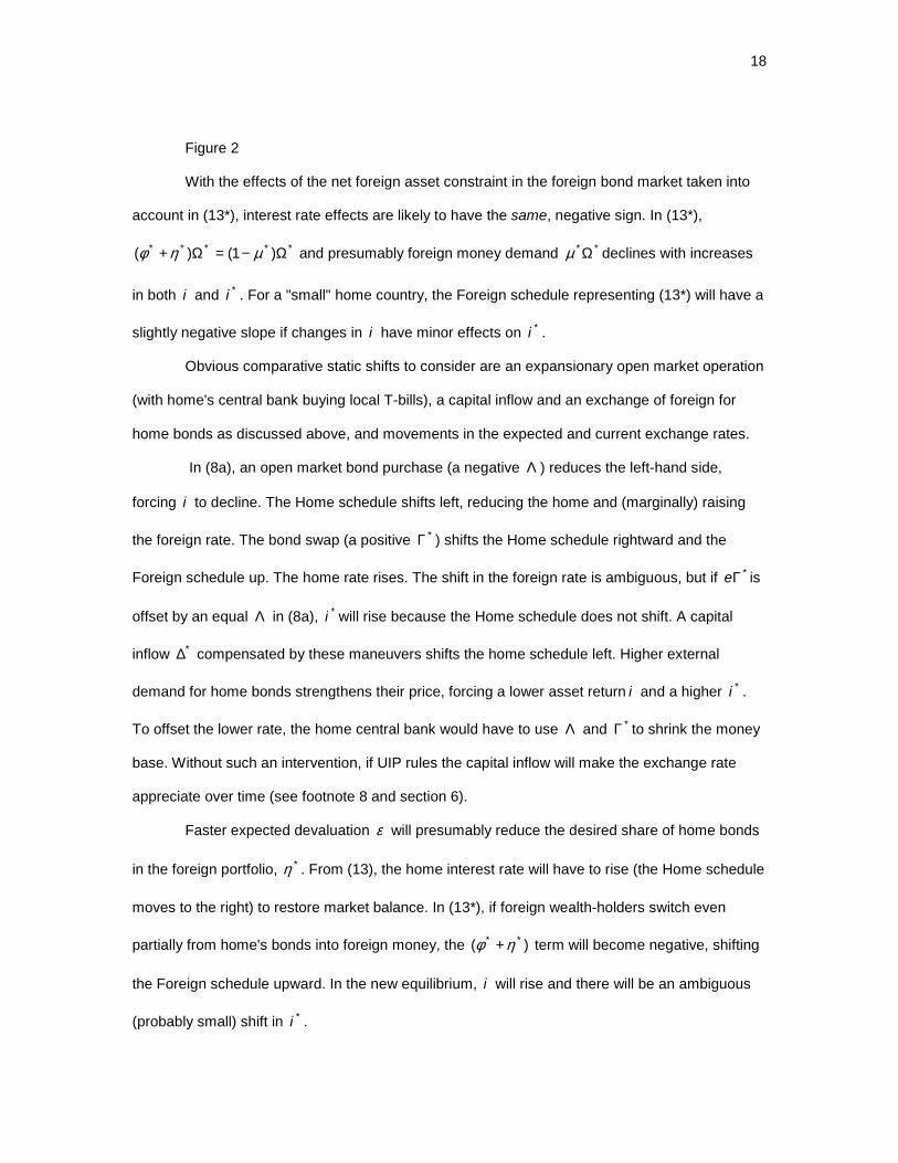
Figure 2

With the effects of the net foreign asset constraint in the foreign bond market taken into

account in (13*), interest rate effects are likely to have the same, negative sign. In (13*),

***** )1()( Ω−=Ω+ µηφ and presumably foreign money demand **Ωµ declines with increases

in both i and *i . For a "small" home country, the Foreign schedule representing (13*) will have a

slightly negative slope if changes in i have minor effects on *i .

Obvious comparative static shifts to consider are an expansionary open market operation

(with home's central bank buying local T-bills), a capital inflow and an exchange of foreign for

home bonds as discussed above, and movements in the expected and current exchange rates.

In (8a), an open market bond purchase (a negative Λ ) reduces the left-hand side,

forcing i to decline. The Home schedule shifts left, reducing the home and (marginally) raising

the foreign rate. The bond swap (a positive *Γ ) shifts the Home schedule rightward and the

Foreign schedule up. The home rate rises. The shift in the foreign rate is ambiguous, but if *Γe is

offset by an equal Λ in (8a), *i will rise because the Home schedule does not shift. A capital

inflow *∆ compensated by these maneuvers shifts the home schedule left. Higher external

demand for home bonds strengthens their price, forcing a lower asset return i and a higher *i .

To offset the lower rate, the home central bank would have to use Λ and *Γ to shrink the money

base. Without such an intervention, if UIP rules the capital inflow will make the exchange rate

appreciate over time (see footnote 8 and section 6).

Faster expected devaluation ε will presumably reduce the desired share of home bonds

in the foreign portfolio, *η . From (13), the home interest rate will have to rise (the Home schedule

moves to the right) to restore market balance. In (13*), if foreign wealth-holders switch even

partially from home's bonds into foreign money, the )( ** ηφ + term will become negative, shifting

the Foreign schedule upward. In the new equilibrium, i will rise and there will be an ambiguous

(probably small) shift in *i .

19

In both (13) and (13*), dimensionally alert asset-holders will deflate expected

depreciation by the current exchange rate e to create a rate of return e/ε comparable to the

others in the model. For a given ε , a discrete (jump) devaluation of the spot rate e will increase

*η , forcing i to decline and *i to shift either way. These responses could be reversed by

devaluation's effects on various terms in the market balance and net foreign asset equations, but

in keeping with most of the literature we ignore such wealth effects.

Finally, stocks of bonds and the real side of the economy with its transactions demands

notwithstanding, in an extreme case the only relevant arguments in the home asset equation (13)

could be i , *i , e , and ε . Although uncovered interest rate parity applies to expectations about

future values of the spot rate, the literature often postulates that contemporaneous partial

derivatives force these four variables to be related in a UIP form such as 0)/( * =++− eii ε .

Because foreigners know as much about arbitrage as do home-dwellers, this formula would be

their asset market equation too. The whole world would have just one asset relationship. Non-

market or institutional forces would have to set most asset prices and rates of return. This

situation is far from the original goal of the portfolio balance model to determine all financial

variables by contemporary market-clearing only.

4. Mundell-Fleming

Compared to portfolio balance, the Mundell-Fleming model is an accounting mare's nest.

It puts a flow commodity market balance (the IS curve) together with a stock asset market

equilibrium (the LM curve), and throws in part of (2) above as a BP relationship. Will this last

equation be satisfied when commodity and asset markets are in balance?

In this section, the answer is shown to be "Yes," regardless of central bank interventions.

The BP equation is not independent, i.e. there cannot be an external imbalance for an exchange

rate adjustment to remove.

To demonstrate this result, the key assumption is that asset market balances are

satisfied continuously over time, i.e. the existence of stock equilibria implies that flow equilibria

exist as well. The relevant specification is in terms of flow-of-funds relationships from Table 1

20

which when supplemented by terms for capital gains and losses are time-derivatives of balance

sheets in Table 2.9 The equilibrium condition needed from the real side is savings-investment

balance. We will assume that adjustment mechanisms exist to generate the relevant equality in IS

equation (16) below.

To be consistent with the presence of investment in cells (A, 5) and (A*, 5*) of the SAM in

Table 1, private sectors must now be allowed to hold capital stocks. In the home economy the

three asset demand functions (5)-(7) continue to apply, along with a stock demand for capital

0=−Ω qPKκ ,

with 1=+++ κφηµ . The valuation ratio q adjusts to clear this equation, and may also enter as

an argument in the investment demand function. This brusque treatment of capital finance could

be considerably expanded as in Franke and Semmler (1999), but it suffices in terms of our

present preoccupations with the exchange rate and balance of payments.

The immediate task is to show how Mundell-Fleming flow equations relate to portfolio

balance. The following discussion focuses on relationships among the flows in Table 1 and the

definitions of the change in home's net foreign assets in (2). It is consistent with any equilibrium

theory of asset accumulation and portfolio choice - Keynesian, intertemporal optimization, or

otherwise.

The first point to recall is that from (2), foreign savings fS is equal to the current account

deficit,

)]([)]([ ******RTeiXPaRTiaXePS hff ++−++= , (14)

and the flows of funds of the rest of the world with the home economy become

0)]()([ ** =+−++ RTRTeS fhf

&&&& . (15)

Foreign savings and flow capital inflows to home's private sector and central bank are the foreign

country's sources of funds. Flow acquisitions of home's securities by its private sector and banks

are the uses.

21

In other words, fS equals the increase in home's foreign debt ( RTf&& + ) less the increase

in its foreign holdings )( ** RTe h&& + . For this Mundell-Fleming BP relationship to be independent, it

must be possible for the home economy's increase in net foreign assets (the bracketed term in

(15)) to differ from its current account surplus fS− when home and foreign IS and LM

relationships are satisfied. Only in such circumstances will the exchange rate or some other

variable have play to restore the balance of payments to temporary equilibrium.

It is easy to see that this situation normally does not arise. First note that the sum of the

flow of funds in rows (E)-(G) in Table 1 and (15) gives

0=−++ PISSS fgh (16)

or macroeconomic saving-investment balance applies. Because equality in (16) is assumed to be

assured by real side IS equilibrium, only three of the four flows of funds (including (15)) can be

independent relationships. They are further constrained by flow clearing of asset markets. The

relevant equations appear in columns (8)-(10) and (9*)-(10*) in the SAM, together with associated

exchange conversions.

All asset markets can be assumed to clear in flow terms if the interest rates i and *i are

free to adjust, the banks satisfy their flows of funds restrictions, and the results of last section

apply. Then the proof that the balance of payments must clear is trivial. Substitutions through the

flows of funds under the assumption that commodity markets are in equilibrium (i.e. (16) is valid)

immediately produce equation (15).

There is no need for the exchange rate or anything else to vary to ensure that this

equality will hold. In the textbook diagram, BP always passes through the IS/LM intersection,

regardless of the value of e . As in the portfolio balance model, the triple intersection will occur

whether or not central banks use flow transactions such as *Γ& and Λ& (which could be

incorporated in the foregoing accounting in straightforward fashion) to regulate changes in their

holdings of home and foreign bonds.

It may be helpful to explore the implications of this result in more intuitive terms. If

equality did not hold in (15), then in the double-entry bookkeeping of the flows of funds and flow

22

asset balances some other equality would have to be violated. For example, suppose that the

home country is running up external arrears by not meeting contracted payment obligations on

outstanding debt so that the current account surplus fS− falls short of the bracketed term in (15).

There are two possible forms of repercussion on home’s flow asset market balances and flows of

funds. One is that some other flow of funds relationship is not satisfied. The other is that if home’s

domestic flows of funds equalities hold, then some flow asset market balance must fail to clear.

Consider the second case. The obvious counterpart to a non-clearing balance of

payments is the domestic bond market in columns (9) and (10*) and rows (L) and (L*) of the

SAM. The run-up in external arrears would be reflected into a flow excess supply of home bonds -

foreigners are not picking up enough domestic securities to provide home the wherewithal to

meet its external obligations. Under such circumstances (as discussed above), a spot devaluation

of appropriate magnitude could be expected to erase the excess supply through a substitution

effect and remove the disequilibrium.

The rub is that if home's other financial markets are in equilibrium then this sort of

adjustment is unnecessary - we know from the analysis of the portfolio balance model that if the

home money market clears then so will the market for bonds. And with both money and bond

markets in balance, there is no room in the accounting for an open balance of payments gap.

The other possibility is that the non-clearing balance of payments is reflected into another

flow of funds relationship subject to the equilibrium condition (16). For example, one can imagine

and even observe - as in recent Asian, Latin American, and Russian experiences - situations in

which the home country is running up external arrears at the same time as the domestic private

sector is undertaking investment projects that aren’t working out (the sum of the terms in row (E)

exceeds zero). An exchange rate realignment might even reverse such simultaneous build-ups of

external and internal bad debt. But at the macroeconomic level such situations are unusual. A

normal, well-regulated banking sector at home is not in the business of providing non-performing

loans to corporations. In harmonious times, the balance of payments emerges automatically from

output and asset market equilibria.

23

Finally, taking exchange rate movements into account, net foreign assets evolve

according to the relationship

)()()( **** RTeRTRTeN hfh +++−+= &&&&&& . (17)

If N& were pre-determined, then (17) could be treated as an "extra" equation to be solved for e& in

a "floating rate" case in which central banks use flow interventions like *Γ& and Λ& to control *R&

and R& . But in line with the discussion of (1) above, there are no obvious economic forces that

would make N& anything but the passive sum of the variables on the right-hand side. Even if N&

were pre-determined, faster capital inflows fT& in (17) would in counter-intuitive fashion speed up

exchange rate depreciation e& . The usual Mundell-Fleming floating rate story does not emerge

naturally from consistent stock-flow accounting.

5. IS/LM comparative statics

The model thus reduces to linked IS/LM systems for the two countries. Financial markets

are described by equations (8a) and (13*), which clear (after home central bank interventions and

other shocks) via adjustments in i and *i . Commodity markets are described by (16) and its

analog in the foreign country. Saving and investment functions can be assumed to respond to the

usual variables - interest rates, activity levels, profit rates emerging from the technology and

institutions underlying V and *V , perhaps q and *q , and so on.

For present purposes, it makes sense to see how a Keynesian version behaves, with

activity levels in both countries determined by effective demand. Because BP equations are not

independent, the spot exchange rate has to be taken as a pre-determined variable in the short

run. We also assume that the home country is "small" in commodity markets, in that the foreign

country's reserves stay constant, and in the sense of Figure 2.

Table 3 gives signs of responses of commodity excess demand and bond excess supply

functions to the endogenous variables - output levels X and *X and interest rates i and *i in

the two-country model - as well as to e and ε . The IS row shows that as usual home excess

demand is reduced by increases in both X and i . Higher foreign output *X stimulates home

24

demand via exports while changes in the foreign interest rate *i are assumed to have no direct

effects. In line with the possibility of contractionary devaluation (Krugman and Taylor, 1978), a

higher value of e may either reduce or increase home's aggregate demand. Faster expected

depreciation ε has no direct effect.

Table 3

In the LM row, by increasing transactions demand for money, a higher X raises the

excess supply of home T-bills, while a higher i cuts it back. Increases in *X and *i also raise

excess supply, while e and ε have the effects discussed in connection with Figure 2. Foreign

IS* and LM* schedules are not affected by output and interest rate changes in a small home

country, and the remaining signs in the last two rows are analogous to those already discussed.

Given the assumptions of Table 3, it is easy to work out how X and i respond to the

other variables. (For simplicity, we consider only direct effects of e and ε in the IS and LM rows,

without solving though IS* and LM*.) Increases in both *i and ε reduce X and raise i . Even if

home and foreign bonds are close substitutes in home portfolios as in Figure 2, it will be true that

1/ * <∂∂ ii because the fall in X reduces excess supply of T-bills. A higher *X puts pressure on

home financial markets and bids up i . The effect on X is ambiguous - increased export sales vs.

domestic demand contraction due to a higher interest rate.

If devaluation is expansionary, a higher e raises X but has an ambiguous impact on i .

The interest rate will rise if the output increase is strong and/or the wealth and substitution effects

of devaluation on home asset equilibrium are weak. A weaker currency is supposed to take

pressure off interest rates, but that outcome does not have to happen.

If devaluation is contractionary, it unambiguously reduces i . The feedback effect on

effective demand leaves the final response of X unclear. Exchange appreciation in this case will

be associated with a higher interest rate and possibly a reduction in output. Strong exchange

rates, high interest rates, and slow growth have been characteristic of many semi-industrialized

25

economies in the 1990s. If the fall in e is the driving force (perhaps because exchange

appreciation is pursued as an anti-inflationary tool), the output and interest rate responses may

reflect a situation in which effective demand is reduced or not strongly stimulated by devaluation.

So what happens to the balance of payments while these changes are going on? As in

the portfolio balance model, reserve changes (as manipulated by central banks) will be the

accommodating variables in both countries when their current accounts (driven largely by IS

adjustments and interest rate changes) and holdings of external T-bills (driven by portfolio

choices) shift over time. In the medium run, the current account will be the "autonomous"

component of the balance of payments, so long as asset markets clear smoothly. Unless foreign

portfolio preferences shift away from home's T-bills as its current account deficits or debt-service

obligations become "too large," there is nothing in the model to prevent a country from running an

external deficit indefinitely. Perhaps the United States since the 1980s is a case in point.

6. UIP and Dynamics

To summarize the last three sections, the exchange rate is not set by temporary macro

equilibrium conditions. It must evolve over time subject to rules based on expectations about its

values in the future. In a world of shifting and perhaps unstable expectations, no simple dynamic

theory is likely to emerge. The best candidate is UIP and it does not reliably fit the data.

However, because UIP relies on arbitrage arguments which "should be true" and has interesting

dynamic properties, a scenario based upon it is worth sketching as an illustration of the sorts of

results that a standard hypothesis can generate in conjunction with a demand-driven IS/LM-

based growth model operating along Keynesian lines. Of course, other model "closures" or

causal structures are possible.10

Under myopic perfect foresight (or MPF) about changes in the exchange rate

with dtdee /== &ε , the UIP formula (3) or (4) can be restated as a differential equation

)( *iiee −=& . (18)

In the two-country IS/LM system the interest rates i and *i are functions of the exchange rate and

other variables. A long-run "equilibrium" rate e , which may or may not easily be attained, is

defined by the condition *ii = .

26

Together with the IS/LM model, (18) makes up a well-defined dynamic system. On the

right-hand side, i and *i are functions of e , e& , and other variables Q , so (18) becomes

),,( Qeefe && = . This equation can be converted to the standard form ),( Qege =& . Assuming MPF, if

the portfolio balance model really did have three independent equations among i , *i , e , e& , and

other variables, it would itself be a dynamic system for the exchange rate, inconsistent in general

with UIP (not to mention full intertemporal arbitrage and optimization).11

Differential equations incorporating MPF in growth and financial models are usually

unstable. An asset price feeds back positively into its own rate of growth, giving rise to saddlepath

dynamics (under appropriate transversality conditions) or a bubble. However, at an initial

equilibrium at which *ii = and ee = , 0/ <deed & in (18) if devaluation reduces the home interest

rate as discussed above. This local stability opens up possibilities for cyclical exchange rate

dynamics not present in most MPF formulations.12

Before turning to that, however, it is worth noting how UIP supports standard Mundell-

Fleming conclusions. From the comparative statics discussed above, a capital inflow with the

money supply held constant is likely to make i fall and *i rise. If the differential equation (18) is

stable, the exchange rate will decline over time, driving the interest rates back together. The

"floating rate" scenario of a capital inflow leading to appreciation applies dynamically, except that

e is not floating in the traditional sense, but is being determined in forward markets via UIP.

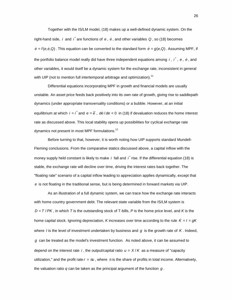
As an illustration of a full dynamic system, we can trace how the exchange rate interacts

with home country government debt. The relevant state variable from the IS/LM system is

PKTD /= , in which T is the outstanding stock of T-bills, P is the home price level, and K is the

home capital stock. Ignoring depreciation, K increases over time according to the rule gKIK ==&

where I is the level of investment undertaken by business and g is the growth rate of K . Indeed,

g can be treated as the model's investment function. As noted above, it can be assumed to

depend on the interest rate i , the output/capital ratio KXu /= as a measure of "capacity

utilization," and the profit rate ur π= , where π is the share of profits in total income. Alternatively,

the valuation ratio q can be taken as the principal argument of the function g .

27

The time derivative of T is iTPKT += γ& where γ is the government's "primary deficit"

(outlays apart from interest payments less revenue) as scaled to the value of the capital stock.

Using the foregoing information, a differential equation for D becomes

DgPiD ])ˆ[( −−+= γ& , (19)

where PPP /ˆ &= is the inflation rate. The steady state value of the debt/capital ratio is

)]ˆ(/[ PigD −−= γ . As is well-known, an economy with 0>γ can only sustain a stable

debt/capital ratio when its capital stock growth rate exceeds the real rate of interest. This

condition has tended to fail recently in industrialized economies (and fail strongly in developing

debtor countries such as Argentina!). We will assume, however, that at least some of the time

g can exceed ( Pi ˆ− ).

Another complication is that the components of the bracketed term on the right-hand side

of (19) depend on D. A higher value is analogous to an increase inT in (8). Excess supply of T-

bills goes up, forcing their interest rate i to rise. In most IS/LM models with an inflation equation

adjoined, the inflation rate P and growth rate g would go down. The derivative of the bracketed

term in (19) with respect to D would be positive, which could make the total derivative

dDDd /& positive around a steady state with 0>D . This potentially unstable case is the focus of

the following discussion.

Effects of the exchange rate e on D& in (19) go through the interest rate directly, as well

as through shifts in g and P induced by interest and output changes. If 0/ <∂∂ ei in the IS/LM

system, we get a direct negative impact of e on D& . If the inflation and growth rates rise with a

lower i , it is clear that 0/ <deDd & . Finally, because a higher D increases i , 0/ >dDed & in (18).

Figure 3 is a phase diagram for the system (18)-(19) in which there is a chance for

cyclical stability. The initial equilibrium at which 0== eD && resides at point A. Suppose that there

is a permanent monetary expansion, driving down i . To bid up the interest rate again, D would

have to rise and e to fall. The curves shift as illustrated.

28

Figure 3

Along the dynamic trajectory, the lower interest rate initially sets off exchange

appreciation and a declining debt/capital ratio. The falling exchange rate begins to push up the

interest rate, increasing the bracketed term in (19) until D starts to rise at point B. Both variables

are now putting upward pressure on the interest rate. When i rises above *i in (18), the

exchange rate begins to depreciate. The trajectory may or may not converge to the new

equilibrium at E.13 Even if it does, the economy is likely to go through cycles. An initial monetary

contraction would create a depreciation-then-appreciation exchange rate history. Since the late

1970s, the secular US external deficit has been accompanied by (so far) two such cycles with

periods exceeding 10 years.

7. Conclusions

One should not take results from a two-dimensional dynamic system too seriously, but

the foregoing narrative illustrates that a properly specified open economy macro model does

contain interesting possibilities. Moreover, they would carry over to intertemporal models which

incorporate UIP, but replace effective demand with Say's Law and derive a private savings (=

investment) rate from a Ramsey-style dynamic optimization. Even with these changes,

intertemporal models have to satisfy accounting relationships like those in Tables 1 and 2. Their

dynamics cannot be less complicated than the trajectory of Figure 3, and as sketched in footnote

12, outright instabilities are also possible. There is no reason to expect monotonic or saddlepoint

"stability."

This observation differs strikingly from early predictions based on the portfolio balance

and Mundell-Fleming models. In one familiar example based on the former, suppose that the

home country runs a current account deficit. Its reserves will fall, leading to monetary contraction

and a higher interest rate. If UIP applies, the exchange rate will depreciate over time, presumably

leading to a better trade performance and a new long-run equilibrium in which the current account

is balanced and exchange and interest rates are stable. In the traditional model "... stock-flow

29

adjustments in the presence of capital mobility will generally move the exchange rate in the right

direction to eliminate a current account deficit in the long run" (Blecker, 1999, p. 57).

This comforting story follows the pattern of Hume's price/specie flow chronicle in

asserting that the existence of a current account deficit stimulates price adjustments such as

depreciation that will make the deficit disappear. But in fact, there is no reason for such

adjustments to happen. In (18), a floating exchange rate has no fundamentals such as a real rate

of return or a trade deficit that can make it self-stabilizing.

As one referee observed, this observation helps explain why "... all fundamentals-based

exchange rate models ... were doomed to fail empirically." The evidence is well summarized by

Frankel and Rose (1995). Although most of the emphasis herein has been on Keynesian

specifications, points raised above apply to widely used monetarist econometric models as well.

They usually start out correctly by postulating just two equations linking money demand to the

interest rate and price level in the home and foreign countries (the exchange rate and its

expected change are not included as arguments in these functions, though from the analysis

herein they should be). The models add the assumption that money markets clear via price

adjustments with supplies pre-determined, i.e. price levels are set by the equation of exchange

modified for interest rate effects. Purchasing power parity is then used as an "extra equation" to

determine the exchange rate from the two national price levels. Because neither a tight link

between an economy's money supply and its price level nor PPP is ever strongly supported by

the data, it is scarcely surprising that these formulations failed. Similar observations apply to

extensions based on UIP, rational expectations, gradual price adjustment, etc.

The bottom line is that e can only float against its own expected future values and

interest rates. In the real world such expectations are determined in part by intrinsically

unpredictable and non-rational forces. In open economy macroeconomics more generally, having

one temporary equilibrium condition fewer than has been supposed opens up a range of

possibilities for exchange rate determination. They should be explored.

30

Notes

1. Unrealistically, the private sector in each country is assumed to hold only the local

money. It is straightforward to deal with the general case by using more symbols, but the SAM

already has too many!

2. Other specifications such as treating imports as negative exports or additional

components of consumption demand are possible, but would not change the main results to be

presented below.

3. For the moment, ε can be interpreted in a Keynesian sense as summarizing the

market's perceptions or views about how the exchange rate is likely to shift over time; a more

contemporary interpretation in terms of myopic perfect foresight appears in section 6 below. Also

note that ε stands for an absolute as opposed to a percentage change per unit of time in e (the

latter interpretation appears frequently in the literature)

4. The macro relationships that must be considered in the contemporary world relate to

both the current and capital accounts. Before and in the first decades after World War II, it made

sense to concentrate only on the trade account. A model proposed 40-odd years ago by Salter

(1959) and Swan (1960) does contain a plausible exchange rate fundamental - the traded/non-

traded goods price ratio. As far as trade is concerned, the exchange rate can be interpreted as

becoming increasingly over-valued when this internal price ratio falls. But for the industrialized

countries at least, payments related to trade are now such a tiny share of total external

transactions that the model is obsolete (Eatwell and Taylor, 2000). In turn, Salter-Swan was the

culmination of a long string of models of the trade account, which assumed that capital flows were

exogenous. They included an elasticities approach (featuring "Marshall-Lerner conditions" on

trade elasticities), an absorption approach, and analysis of internal vs. external balance which led

to Salter-Swan. A monetary approach to the balance of payments worked out in the 1950s and

1960s fed into the portfolio balance and Dornbusch models discussed below, as well as many

econometric attempts to predict shits in the spot rate (see section 7). Williamson and Milner

(1991) is a solid mainstream summary of all this history.

31

5. We stick with the standard literature in assuming that the monetary authorities

intervene to control their holdings of assets. A Post Keynesian scenario in which interest rates are

set exogenously and money supplies adjust would be straightforward to work through.

6. The diagram presupposes that the home country is a net creditor at the ruling

exchange rate. To get to the net debtor case, the External assets schedule can be rotated

clockwise via exchange appreciation until it crosses the vertical axis above the origin.

7. Another way is to linearize three asset market balance equations around an initial

equilibrium and attempt to solve them for "small" changes in i, *i , and e , subject to the

accounting restrictions mentioned in the text. After great labor, the Jacobian matrix of this system

will turn out to be singular. Such an exercise was the genesis of this paper.

8. The interest rate changes could induce shifts in the exchange rate over time. On the

basis of the comparative static results below, it seems likely that the compensated capital inflow

discussed in the text will make i fall and *i rise. Under UIP and myopic perfect foresight (section

6), the exchange rate would tend to appreciate, 0<e& .

9. To keep the analysis simple, all variables are assumed to be continuously

differentiable functions of time. In practice, both stock and flow variables can change

discontinuously. But if in so doing they obey all relevant balance sheet and income statements,

the transition from portfolio balance to Mundell-Fleming accounting goes through. The extensive

theory and notation required to deal with such eventualities as well as changes in prices is best

avoided here. Foley (1975) and Burgstaller (1994) take up the complications. In theory,

accounting consistency between stock and flow variables is a means for linking the future to the

present; in practice (in discrete time) it will be observed in sectoral balance sheet and flow of

funds accounts because they are constructed that way.

10. For example, both the well-known model by Dornbusch (1976) and the one herein

stand on IS and LM (but not BP) foundations. But for Dornbusch, output is set by Say's Law

(perhaps transiently relaxed by "sticky price" short-term output dynamics); the money market

balance is combined with UIP and regressive exchange rate expectations around purchasing

power parity or PPP (an "extra equation") to make e depend on the real money supply M/P;

32

changes in P over time are driven by the difference between aggregate demand and output; and

since this difference is non-zero away from the steady state the short-run current account is

endogenous and implicitly offset by capital flows or reserve movements which are sterilized to let

the central bank control M. Because it obeys PPP and the quantity theory in the long run, the

model is much more closely tied to "fundamentals" than the one presented in the text.

11. As observed by Branson and Handerson (1985), there were many papers in the

1970s and early 1980s devoted to dynamic analysis of a portfolio balance model augmented by

IS and BP relationships. A typical "finding" was that the dynamic system could be unstable if

home country net foreign assets were negative. Unfortunately this literature was flawed because

it assumed the spot rate could be set by portfolio balances and also treated the BP equation as

being an independent restriction on the dynamic system.

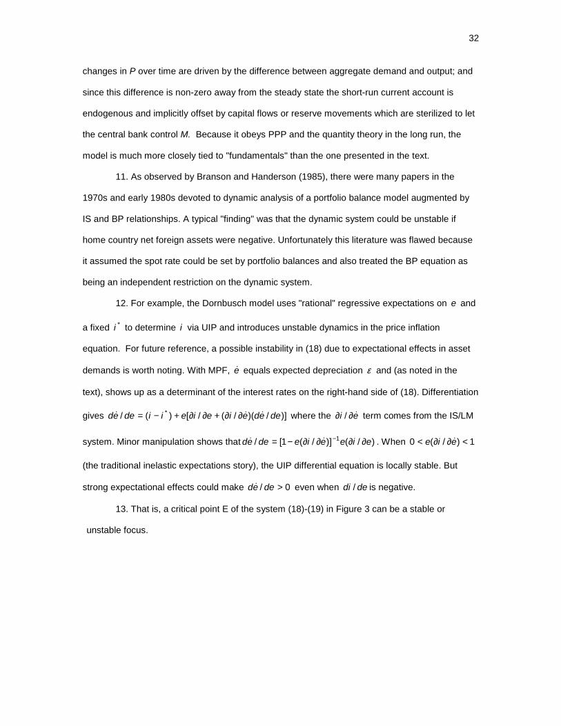
12. For example, the Dornbusch model uses "rational" regressive expectations on e and

a fixed *i to determine i via UIP and introduces unstable dynamics in the price inflation

equation. For future reference, a possible instability in (18) due to expectational effects in asset

demands is worth noting. With MPF, e& equals expected depreciation ε and (as noted in the

text), shows up as a determinant of the interest rates on the right-hand side of (18). Differentiation

gives )]/)(/(/[)(/ * deedeieieiideed &&& ∂∂+∂∂+−= where the ei &∂∂ / term comes from the IS/LM

system. Minor manipulation shows that )/()]/(1[/ 1 eieeiedeed ∂∂∂∂−= −&& . When 1)/(0 <∂∂< eie &

(the traditional inelastic expectations story), the UIP differential equation is locally stable. But

strong expectational effects could make 0/ >deed & even when dedi / is negative.

13. That is, a critical point E of the system (18)-(19) in Figure 3 can be a stable or

unstable focus.

33

References

Blecker, Robert A. (1999) Taming Global Finance: A Better Architecture for Growth and Equity,

Washington DC: Economic Policy Institute

Blecker, Robert A. (2002) "Capital Mobility, Macroeconomic Imbalances, and the Risk of Global

Contraction," in John Eatwell and Lance Taylor (eds.) International Capital Markets:

Systems in Transition, New York: Oxford University Press

Branson, William H., and Dale W. Henderson, "The Specification and Influence of Asset Markets"

in Ronald W. Jones and Peter B. Kenen (eds.) Handbook of International Economics,

Vol. 2, Amsterdam: North-Holland

Burgstaller, Andre (1994) Property and Prices: Towards a Unified Theory of Value, New York:

Cambridge University Press

Dornbusch, Rudiger (1976) "Expectations and Exchange Rate Dynamics," Journal of Political

Economy, 84: 1161-1176

Eatwell, John, and Lance Taylor (2000) Global Finance at Risk: The Case for International

Regulation, New York: New Press

Fleming, J. Marcus (1962) "Domestic Financial Policies under Fixed and Floating Exchange

Rates," IMF Staff Papers, 9: 369-379

Foley, Duncan K. (1975) "On Two Specifications of Asset Equilibrium in Macroeconomic Models,"

Journal of Political Economy, 83: 303-324

Foley, Duncan K., and Miguel Sidrauski (1971), Monetary and Fiscal Policy in a Growing

Economy, New York: Macmillan

Franke, Reiner, and Willi Semmler (1999) "Bond Rate, Loan Rate, and Tobin's q in a Temporary

Equilibrium Model of the Financial Sector," Metroeconomica, 50: 351-385

Frankel, Jeffrey A., and Andrew K. Rose (1995) "Empirical Research on Nominal Exchange

Rates" in Gene Grossman and Kenneth Rogoff (eds.), Handbook of International

Economics, Vol. 3, Amsterdam: North-Holland

34

Godley, Wynne (1996). "A Simple Model of the Whole World with Free Trade, Free Capital

Movements, and Floating Exchange Rates." Unpublished manuscript, The Jerome Levy

Institute, Bard College

Isard, Peter (1995) Exchange Rate Economics, Cambridge: Cambridge University Press

Kareken, John, and Neil Wallace (1981) "On the Indeterminacy of Equilibrium Exchange Rates,"

Quarterly Journal of Economics, xx: 207-222

Keynes, John Maynard (1923) A Tract on Monetary Reform, London:Macmillan

Keynes. John Maynard (1936) The General Theory of Employment, Interest, and Money, London:

Macmillan

Krugman, Paul, and Taylor, Lance (1978), "Contractionary Effects of Devaluation." Journal of

International Economics vol. 8, pp. 445-456

Mundell, Robert A. (1963) "Capital Mobility and Stabilization Policy under Fixed and Flexible

Exchange Rates." Canadian Journal of Economics and Political Science, 29: 475-485

Obstfeld, Maurice, and Kenneth Rogoff (1995) "The Intertemporal Approach to the Current

Account" in Gene Grossman and Kenneth Rogoff (eds.), Handbook of International

Economics, Vol. 3, Amsterdam: North-Holland

Ramsey, Frank P. (1928) "A Mathematical Theory of Saving," Economic Journal, 38: 543-559

Rosensweig, Jeffrey A., and Lance Taylor (1990) "Devaluation, Capital Flows, and Crowding-Out:

A CGE Model with Portfolio Choice for Thailand" in Lance Taylor (ed.) Socially Relevant

Policy Analysis, Cambridge MA: MIT Press

Salter, W. E. G. (1959) "Internal and External Balance: The Role of Price and Expenditure

Effects," Economic Record, 35: 226-238

Swan, Trevor (1960) "Economic Control in a Dependent Economy," Economic Record, 36: 51-66

Tobin, James (1969) "A General Equilibrium Approach to Monetary Theory," Journal of Money,

Credit, and Banking, 1: 15-29

Williamson, John, and Chris Milner (1991) The World Economy, New York: New York University

Press

35

Table 2: Balance Sheets for Two Countries

Home Country

Private Sector Banking System Government

M Ω bT M T

hT *eR

*heT

qPK

Foreign Country

Private Sector Banking System Government

*M *Ω *bT *M *T

*fT eR /

eTf /

*** KPq

Table 3: Signs of Market Responses in a Linked IS/LM Model

X i *X *i e ε IS - - + 0 ± 0 LM + - + + - + IS* 0 0 - - ± 0 LM* 0 0 + - + -

36

Foreign external assets extT External assets slope e= extT eN / *

extT Home external assets *extT

N− Figure 1 Determination of net foreign assets from initial external holdings

37

Foreign interest rate *i Foreign A B Home Home interest rate i Figure 2 Effects of devaluation of the home currency. Home monetary expansion is similar, except that only the Home schedule shifts.

38

Debt/capital ratio D D E C A 0=e& B 0=∆& Exchange rate e

Figure 3 Adjustment dynamics for the exchange rate and debt/capital ratio after a "permanent" monetary expansion.

Table 1: A Two-Country SAM with Trade and Current home expenditures Home ext. receipts Changes in home claims Exchange conversions Output Cap. Foreign Home For. For. Home Costs Private Gov’t. Banks form. Exports interest Money bonds bonds Totals to Home to For. (1) (2) (3) (4) (5) (6) (7) (8) (9) (10) (11)

Output (A) PC PG PI ** XPa PX Incomes

Private (B) V hiT bΠ **hTei hY

Gov't. (C) hYτ gY

Banks (D) biT **Rei bY Flows of funds

Private (E) hS PI− M&− hT&− *hTe &− 0

Gov't. (F) gS T& 0

Banks (G) 0 M& bT&− *Re &− 0 External

Imports (H) aXeP * e

Exports (I) ** XPa− e/1

Int. in (J) **extTei− e

Int. out (K) extiT e/1

Change (L) extT&− e/1 in ext. liab.

Change (M) *extTe & e

in ext. assets Totals (N) PX hY gY bY 0 0 0 0 0 0

Interest Flows and International Capital Movements Current foreign expenditures Foreign ext. receipts Changes in foreign claims Output Cap. Home For. Home Costs Private Gov’t. Banks form. Exports interest Money bonds bonds Totals (1*) (2*) (3*) (4*) (5*) (6*) (7*) (8*) (9*) (10*) (11*)

**CP **GP **IP aXP * ** XP (A*) Output Incomes

*V **fTi *

bΠ eiTf / *fY (B*) Private

**fYτ *

gY (C*) Gov't.

**bTi eiR / *

bY (D*) Banks Flows of funds

*fS **IP− *M&− *

fT&− eTf /&− 0 (E*) Private

*gS *T& 0 (F*) Gov't

0 *M& *bT&− eR /&− 0 (G*) Banks

External

aXP *− (H*) Exports

eXPa /** (I*) Imports

**extTi (J*) Interest out

eiText /− (K*) Interest in

eText /& (L*) Change in ext. assets

*extT&− (M*) Change in ext. liab.

** XP *fY *

gY *bY 0 0 0 0 0 0 (N*) Totals