Exchange Rates and Local Labor Markets - Federal Reserve Bank

0

Exchange Rates and Local Labor Markets

Linda Goldberg and Joseph Tracy

Federal Reserve Bank of New York and NBER

ABSTRACT

We document the consequences of real exchange rate movements for the employment, hours,

and hourly earnings of workers in manufacturing industries across individual states. Exchange

rates have statistically significant wage and employment implications in these local labor

markets. The importance and size of these dollar-induced effects vary considerably across

industries and are more pronounced in some U.S. regions. In addition to the importance of

exchange rate shocks, we confirm prior research results showing that relatively strong local

conditions drive up wages, in local industries, while anticipated future (positive) local shocks

reduce current wages.

January 25, 1999 revision

JEL codes: F31, F3, F4, J30, E24

The views expressed in this paper are those of the individual authors and do not necessarily reflect the positionof the Federal Reserve Bank of New York or the Federal Reserve System. Address correspondences to Linda S.Goldberg or Joe Tracy, Federal Reserve Bank of NY, Research Department, 33 Liberty St, New York, NY10045. fax: 212-720-6831; email: [email protected] or [email protected] . Jenessa Guntherand Henry Schneider provided valuable research assistance. We appreciate the useful comments of AndrewRose, Jane Little, Jose Campa, and participants of the NBER Conference on Trade and Wages in MontereyCA, February 1998.

1

I. Introduction

With the increased internationalization of the U.S. economy, the implications of dollar

movements for workers has emerged as a pressing question. A literature has developed that

considers this and related themes. First, the exchange-rate pass-through literature discusses

the degree to which prices of goods -- whether exported, imported, or produced domestically

for home consumption -- are influenced by exchange rates. In the United States export prices

tend to be fairly stable in dollar terms. Import prices appear to be more responsive to

exchange rates movements, but this responsiveness varies considerably across types of goods

and across trading partners. Import-competing products show much smaller elasticities of

response to exchange rates.1 Exchange rates also matter for producer profitability, and for

decisions about capital spending and employment. Industry features –such as their trade

orientation and competitive structure -- scale the importance of these exchange rate effects.2

The labor market effects of exchange rates are an open question. For the United

States, analyses using data through the mid-1980s show that exchange rates have had

significant implications for wages (Revenga 1992) and for employment across manufacturing

industries (Branson and Love 1988).3 A recent cross-country, cross-industry study by Burgess

and Knetter (1996) found statistically significant effects of exchange rates for employment,

with the size of these effects related to industry characteristics such as competitive structure.

However, recent work by Campa and Goldberg (1998) found weaker implications of

exchange rates for employment in U.S. industries, but more pronounced effects for wages.

This study used a longer time series than previous empirical work (about twenty-five years of

annual data) and focussed on two-digit industry employment, wages, overtime activity and

overtime wages. The testing methodology allows for exchange rate transmission channels to

vary over time with industry trade exposures to exchange rates through both revenues and

1See Goldberg and Knetter (1997) for a survey. The distribution of exchange rate elasticities of the set ofUnited States import prices thus far examined appears to be centered around 0.5, but the set of goods studied isby no means exhaustive.2See Clarida (1997) and Sheets (1996) on profitability and exchange rates. Campa and Goldberg(forthcoming) show that investment spending is time-varying in accordance with the export and importedinput orientation of producers across various industries and across countries and is strongest in industries withlow price-over-cost markups (which can be viewed as closer to perfectly competitive market structures).

2

costs. Exchange rate effects were statistically significant mainly for wages, and strongest in

industries that are more trade oriented and in industries that generally have lower profit

margins.

The combination of significant wage responsiveness to exchange rates, without

comparable employment effects poses some interesting questions. One possible reconciling

argument is that a dollar appreciation, for example, could lead workers to lose their jobs, but

then be re-employed at lower wages within the same broad industry group but in a different

narrower industry definition. Such findings would be consistent with observed patterns of

labor force adjustment to oil price shocks (Davis and Haltiwanger, 1997). If this is the case, a

related question is whether workers take new positions in a similar industry within a local

labor market, or if they look for opportunities in a similar industry elsewhere in the country.

Employment changes can entail worker relocation as well as the type of wage adjustments

from moving within and across manufacturing industries that have been detailed by Revenga

(1992). Another argument is that under adverse employment conditions from a dollar

appreciation, for example, workers may engage in less on-the-job search for better paying

jobs.4 Under these conditions, one might observe relatively stable employment with magnified

wage restraint. By unraveling these issues, we hope to better understand the degree of labor

market disruption associated with dollar fluctuations.

The present paper examines more than two decades of data on average hourly

earnings, hours, and employment for 2-digit industries located within the individual states of

the United States. This approach has several advantages over prior studies. First, since the

trade orientation of industries varies by industry location, we are able to better identify the

magnitude of currency shocks hitting local industries. Second, we are able to consider the

spillovers of exchange rate effects across local industries. From a local labor market

perspective, such spillovers may help explain the magnified wage responses and reduced

employment sensitivity to exchange rates. Third, by examining state-level data, we capture

3Examining the 1970s into the early 1980s, Branson and Love estimate that durable goods producers had jobswere most responsive to exchange rates. Using Revenga’s computed elasticities, the estimated effects on jobsare increasing gradually to the extent that import competition exists in an industry.4 See Mortensen (1986) for a discussion of on-the-job search models.

3

the adjustments made by workers who might move across state lines, yet remain within the

same broad industry.

We find that real exchange rates contribute significant explanatory power to

regressions on average hourly earnings, hours, and employment. In pooled industry

regressions, dollar appreciations (depreciations) are associated with small but statistically

significant declines (increases) in hourly earnings by workers. In individual industry

regressions, we observe significant variability across industries in the levels of these earnings

implications and even in the sign of these effects. Moreover, even within individual industries,

some regions are particularly sensitive to dollar movements. Cross-industry spillovers, which

we interpret as providing an indirect means of worker exposure to exchange rates, are

significant for average hourly earnings and for employment within high-markup industries.

In contrast with results drawn from nationally-aggregated data for industries, the state-

level data exhibit more pronounced responsiveness of employment and hours worked within

industries. On balance, dollar appreciations (depreciations) are associated with employment

declines (increases) for high- and low- profit-margin industry groups. As industries increase

their export orientation, the adverse consequences of appreciations for employment also

increase. However, some of these adverse consequences are counteracted as industries

increase their reliance on imported inputs. Both forces are significant in determining the

employment effects of exchange rates, and they differ qualitatively and quantitatively across

regions and across industries.

Finally, our analysis also focuses on and confirms the type of dynamic patterns of

adjustment in local labor markets previously reported by Topel (1986). Using Topel’s

methodology, we construct state- and industry-specific relative demand shocks, both actual

and anticipated. Similar to Topel’s finding using micro date, we find that wages increase in

response to current relative demand shocks and decrease in response to expected future

relative demand shocks.

4

II. The Theory

Our theoretical set-up pairs a model of dynamic labor demand and exchange rate

exchange rate exposure (Campa and Goldberg 1998) with a dynamic local labor supply

specification. The theory shows clear reasons why industries should be differentially affected

by exchange rates. One reason is that industries differ in trade orientation. But, even

controlling for these differences, exchange rate effects on wages and employment should vary

across industries depending on: (i) the industry product demand elasticity at home and abroad;

(ii ) the initial labor share in production; and (iii ) the elasticity of labor supply facing the

industry in that locality. Industries with high labor demand elasticity with respect to wages

will exhibit more employment response and less wage response to exchange rate movements.

Each industry within each locality (defined as a state in our data) can experience

shocks that alter its wages directly or indirectly.Direct effectsof exchange rates arise through

own-industry trade orientation.Indirect effectsarise through spillovers across local industries

via expected alternative wages. Local unemployment rates are important since they influence

the probability that a worker will be able to find a job that offers the alternative wage. Some

shocks can change the current or future attractiveness of an entire locality and lead to labor

supply shifts through in- or out-migration, as in Topel (1986).

Controlling for direct and indirect effects of exchange rates could help identify the

separate channels for wage and employment responsiveness. For example, if an industry is

export-oriented, in general a dollar appreciation is expected to reduce the competitiveness of

its products, and as a consequence place downward pressure on industry wages and lead to

layoffs. However, if other local industries also are export-oriented, the dollar appreciation can

lower the alternative wage available to workers and locally expand the labor supply to the

initial industry. The offsetting direction of movement in labor demand and labor supply to the

industry may lead to magnified wage effects and muted employment effects.

A. Exchange Rates and Labor Demand:We begin with profit maximizing producers who

sell to both domestic and foreign markets. Producers make decisions in a dynamic and

uncertain environment, and consider the future paths of all variables influencing their

profitability. The unknowns for the producer are aggregate demand in domestic and foreign

5

markets,y andy*, and the exchange rate,e, defined as domestic currency per unit of foreign

exchange. Production uses three factors: domestic laborL, other domestic inputsZ, and

imported inputs,Z*. Respective factor prices are denoted byw, s, and es*. Labor is a

homogeneous input into production and levels of non-labor inputs can be adjusted in the

short-run without additional costs.

Producers optimize over levels of factor inputs and total output in order to maximize

expected profits,π , (equation 1) subject to the constraints posed by the production function

(equation 2) and product demand conditions in domestic and foreign markets (equation 3).

Revenues arise from domestic market sales,q, and foreign market sales,q*. In both markets,

the exchange rate influences demand by altering the relative price of home products versus

those of foreign competitors. The exchange rate also directly enters costs through the

domestic price of imported inputs.

( )

( )( )

( ) ��

�

�

��

�

�

∆−−−−

+= �

∞

=

t

ttttttt

ttttt

tttt

tt

ttt

ttt

Lc

ZsZseLw

qeyqpe

qeyqp

ZZLQeyy

**

*,*:**

,:

,*,,max,*,

0

φπ (1)

subject to Q q q= + * , βααβ −−= 1* ZZLQ , (2)

and ( ) ( ) η/1,,: −= qeyaeyqp and ( ) ( ) */1**,**,:** η−= qeyaeyqep (3)

The time discount factor is defined by τ

τδφ Π=t . In equations (2) and (3) we have dropped

the period t time subscripts for convenience.5 A Cobb-Douglas production structure is

assumed for simplicity, but our main results also will hold under a more general CES

production structure. In equation (3) the parametersη= andη* are the domestic and foreign

product demand elasticities facing producers. The demand curves in domestic and foreign

5 A Cobb-Douglas production structure is assumed for simplicity, but ourmain results also will hold under amore general CES production structure.

6

markets include multiplicative demand shifters,( )eya , and ( )eya *,* , which capture the

influence of real income differences across markets and exchange rates.

It is assumed that an industry’s labor inputL is costly to adjust. We assume quadratic

adjustment costs that are proportional to the prevailing wage in the industry (equation 4). The

parameterb allows for additional industry variation in the cost of adjusting employment levels.

( ) ( )212 −−=∆ tttt LL

bwLc (4)

Following Nickell (1986), the solution of this optimization problem is a dynamic

equation for optimal labor demand, where labor adjusts toward a target level~L that would be

optimal in the absence of adjustment costs. The speed of adjustment of labor demand to~L ,

(1-µ), is reduced when industries face high adjustment costs,b, and have low wage

sensitivity of marginal revenue product. Nickell shows that labor demand in any period can

be approximated by

( )( ) ( )�∞

=+− −−+=

01

~11

jjt

jtt LggLL µδµδµµ (5)

whereg is the rate of real wage growth for an industry. Solving the optimal labor problem of

equations (1) to (4), Campa and Goldberg (1998) show that the labor demand targetL~

is

sensitive to exchange rates, with the effects of exchange rates transmitted through three

separate channels – revenues from home market sales, revenues from foreign market sales,

and costs of imported inputs into production. The elasticity of response ofL~

to exchange

rates is

( )( ) ( )( )( ) ( )( )( )( ) �

�

�

�

��

�

�

∂∂−

+⋅−++⋅++⋅=

∂∂

−

−−−

1

1*11

**

11*1*11~~

ZQes

pepp

e

L

e

Lpeeppe

α

ηηηηχηηβ

(6)

where ( )iiiiiii qpqpqp **** +=χ represents the share of export sales in revenues, and

eppe *andηη are domestic and foreign price elasticities with respect to exchange rates.

Observe that the three groups of terms on the right-hand side of equation (6) correspond to

the three exposure channels: the sensitivity to exchange rates of labor demand through

7

revenues from domestic sales, revenues from foreign market sales, and the costs of

productive inputs. By invoking basic relationships on exchange-rate pass-through

elasticities and ex-ante law of one price, we rewrite this relationship as:

( ) ( ) ( )( )αχηηβ

111 **11~~

−−− ∂∂−+++=∂∂

ZQkMp

e

L

e

L(6’)

Equation (6’) clearly shows the three channels and industry features which magnify

or reduce the degree of industry response to exchange rate movements. First, more import

penetration of domestic markets (M) increases the sensitivity of labor demand to exchange

rates by increasing the price competitiveness of foreign goods. Second, more export-

orientation (m) increases the sensitivity of labor demand to exchange rates, since export

revenues are relatively more responsive to exchange rates. Third, greater reliance on

imported components (higherα) can offset or even reverse the adverse consequences of a

stronger currency (for example) on industry labor demand. Fourth, more labor intensive

production (i.e. highβ) is associated with reduced sensitivity of labor demand to exchange

rates. Finally, industries characterized by greater competition among firms (with lowη or η*)

are expected to have labor demands that are more sensitive to exchange rates.

Using equations (5) and (6’), and introducing log-linearized terms for domestic and

foreign aggregate demand conditions, we generate the following reduced form for optimal

labor demand by an industry.6

( ) ( )��

�

�

��

�

�

+++

++++++−+=

− *654

3,32,31,30,3*

2101

1

tti

tiii

ttiiii

scscwc

ecMcccycyccLL

t

tt

αχµµ (7)

where all variables other thanχ, M, andα are defined in logs.7 All variables and parameters

are specific to an industry except foryt and yt*

.8 Within an industry, state or regional

differences in labor demand may arise from local differences in trade exposures.

6 Changes in foreign currency input costs through foreign wages are absorbed into theα term.

8

B. Labor Supply: Our approach to labor supply focuses on the behavior of forward-looking

workers in a local labor market. These workers choose their labor supply to an industry by

considering the wages offered by that industry relative to the alternative wage (as offered

locally by other industries). Local labor supply also responds to both current and expected

future local demand conditions, all relative to conditions outside of the locality. As Topel

(1986) demonstrates, these conditions can lead to in-migration or out-migration from an area.

A reduced form representation for labor supply to an industryi in a localityr is

( ) trr

tir

tiririr

t yawwaaL 321 ˆ +−+= (8)

where try is a vector of terms for local relative conditions (current relative strength of the

locality, and expected future relative strength), andirw is the alternative wage in industries

outside of industryi in the locality.9 Exchange rates can shift the labor supply curve facing an

industry in a locality through their impact on the alternative wage, with the magnitude of the

shift depending on the trade orientation of the other local industries,irX .10 The likelihood

that industryi workers could get this alternative wage depends on the tightness of local labor

markets. We proxy this tightness as inversely related to the local unemployment rateUnempr.

So, trr

tirr

tir UnempaeXaw ''ˆ 54 +≈ , and we write the new reduced form equation for labor

supply as:

trr

tirr

trr

tirir

t UnempaeXayawaairL 54321 ++++= (9)

7 The actual parameters on the shocks introduced in our equation (7) depend on the perceived degree ofpermanence of the shock. A shock that is transitory will have a much smaller impact on labor demand than ashock that is viewed as permanent.8 Real bilateral exchange rates all are exogenous to an industry. These bilateral exchange rates with currenciesof individual countries are weighted differently for each industry, depending on the importance of a country asthe industry’s trading partner.9 Labor supply is upward sloping in an industry’s wage if there is heterogeneity in the workforce, either interms of preferences for industry job attributes or mobility costs.10 The alternative wage should be viewed as an equilibrium alternative wage, so that it ---in fact--- would be afunction of all of the variables that shift labor demand (as shown in equation 7). Introducing this full set ofterms at this point would complicate notation and have no bearing on our ultimate estimation structure or ourinterpretation of the exchange rate channels. The existence of these other terms would matter for theinterpretation on coefficients on the domestic and foreign income and factor price terms in the regressions ifone were to attempt a semi-structural interpretation of these coefficients.

9

for industryi in a state / regionr.

C. Labor Market Equilibrium: Setting labor demand by a local industry (equation 7) equal

to local labor supply (equation 9) yields equations in industry employment and wages:11

( ) 1764,53,52,51,50,5

63210 *

−++⋅+++++

++++=

tii

tri

tiririiiiiii

trir

ti

ti

tiirir

t

LyeXMX

Unempsyyw

ωωωαωωωωωωωωω

(10a)

( ) 1764,53,52,51,50,5

43210 *

−++⋅+++++

++++=

tii

tr

tiririiiiiii

trir

ti

ti

tiir

tir

LyeXMX

UnempsyyL

λλλαλλλλλλλλλ

(10b)

Equations (10a) and (10b) form the basis for our tests of exchange rate and local demand

effects on the labor market of industryi operating in regionr. The wage and employment response

in an industry to local shocks depends on the elasticities of labor demand and supply, as well as the

costs of adjusting employment in that industry. When labor demand or supply curves are steep –

indicating low employment sensitivity to wages -- shocks to either demand or supply lead to

relatively less employment response and more wage response. When industries have high labor

force adjustment costs, the short-run shift in labor demand in response to any given shock is

smaller. Given an industry’s trade orientation, a more concentrated (and less competitive) industry

will experience a smaller labor demand shift from any given shock.

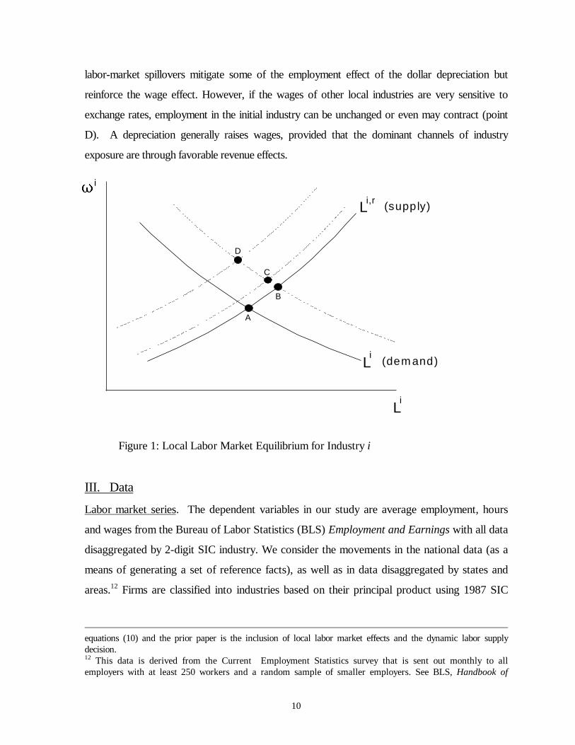
The effects of a dollar depreciation on wage and employment in a particular industry are

illustrated in Figure 1. For an industry with primary external orientation through its export sales, a

dollar depreciation increases labor demand. In the absence of a labor supply shift, labor market

equilibrium moves from point A to point B. Thedirect effectsof the depreciation are expanded

employment and higher wages in the industry. Yet, ifother local industries are also trade-oriented,

labor supply to industryi might contract if alternative wages rise in those other industries. The

decline in labor supply to industryi because of the exposure of other local industries moves the

equilibrium to point C or point D. These indirect effects can be moderate (point C), so that local-

11 The coefficients on the interacted exchange rate terms are interpreted in relation to the individual labor demandand labor supply equations in Campa and Goldberg (1998). The main difference between the current system of

10

labor-market spillovers mitigate some of the employment effect of the dollar depreciation but

reinforce the wage effect. However, if the wages of other local industries are very sensitive to

exchange rates, employment in the initial industry can be unchanged or even may contract (point

D). A depreciation generally raises wages, provided that the dominant channels of industry

exposure are through favorable revenue effects.

Figure 1: Local Labor Market Equilibrium for Industryi

III. Data

Labor market series. The dependent variables in our study are average employment, hours

and wages from the Bureau of Labor Statistics (BLS)Employment and Earningswith all data

disaggregated by 2-digit SIC industry. We consider the movements in the national data (as a

means of generating a set of reference facts), as well as in data disaggregated by states and

areas.12 Firms are classified into industries based on their principal product using 1987 SIC

equations (10) and the prior paper is the inclusion of local labor market effects and the dynamic labor supplydecision.12 This data is derived from the Current Employment Statistics survey that is sent out monthly to allemployers with at least 250 workers and a random sample of smaller employers. See BLS, Handbook of

C

D

A

B

L

L

i,r

i

Li

qi

(supply)

(dem and)

11

classifications. We exclude Alaska, Hawaii, and the District of Columbia from the state data.

The data span 1971 through 1995.

The employment datacapture all persons on establishment payrolls who received pay

for any part of the pay period that includes the 12th day of the month. Proprietors, self-

employed, unpaid volunteers and family workers, and domestic workers are excluded. Persons

on paid vacation or sick leave are counted, as are workers who are unemployed or on strike

for some but not all of the pay period. Thehours datareflect hours paid, which may differ

from scheduled hours or hours worked. Overtime hours and hours paid to workers on

vacation or sick leave are included. Worker absenteeism and work stoppages cause paid hours

to fall below scheduled hours and are not included.

The earningsdata reflect average weekly earnings divided by average weekly hours.

Workers who are not paid weekly have their earnings and hours expressed on a weekly basis.

Earnings reflect payments for all workers who were on the payroll for any part of the pay

period covering the 12th of the month. Gross payroll prior to deductions for social security,

life insurance, tax withholding, and union dues is used. Overtime, holiday, and incentive pay as

well as regular bonus payments are included, while non-regular bonus payments are excluded.

Firm contributions to fringe benefits, such as health insurance and retirement accounts, are not

included.

Exchange rate series. Our empirical work uses export and import real exchange rates for each

industry. These industry-specific real exchange rates are constructed by weighting the bilateral real

exchange rates of U.S. trading partners in accordance with the importance of these partners in

industry exports or imports in each year. To convert nominal exchange rates into real series, the

nominal measures are adjusted by the GDP deflators of the respective trade partners (International

Financial Statisticsdata). The resulting real trade-weighted dollar exchange rates follow the

empirical convention that an increase in the exchange rate corresponds to an appreciation of the

dollar. This convention is opposite that used in our theoretical section.

Methods(1997) for details. This sampling implies that smaller employer response to stimuli may be less wellcaptured by the data set.

12

We use industry-specific exchange rates, rather than a common trade-weighted measure,

because these better reflect the actual shocks to individual industries. The industry-specific series

are generally highly correlated with the overall real exchange rate for the United States (Appendix

Table 1 provides correlation coefficients). However, for some industries the export exchange rates

clearly are more similar to the aggregate real exchange rate measure than are the import exchange

rates. The industry for which the export exchange rate is least correlated with the aggregate

measure is Lumber and Wood Products, with a 0.63 correlation coefficient. On the import index

side, the correlation coefficients between the industry exchange rates and the aggregate real

exchange rate were as low as 0.36 for the Petroleum and Coal Industry, 0.50 for Paper and Allied

Products, and 0.58 for Lumber and Wood Products. Therefore, our industry-specific series are

most relevant for capturing industry-specific shocks to import-competitiveness or imported input

providers.

Industry trade orientation series. In some regression specifications, we interact the real exchange

rates with measures of industry export share and imported input share (Campa and Goldberg, 1997

constructions, based on U.S. Department of Commerce series and U.S. input-output tables). These

industry series are not differentiated across states or regions of the United States.

We are able to perform such state differentiation for our export measures by using a shorter

time series of export data reported by state of origin and by industry, compiled by the

Massachusetts Institute for Social and Economic Research (MISER).13 These series are only

available by 2-digit SIC beginning in 1988. For our regressions, we take this information on the

relative importance of exports to an industry in a state over this shorter time period, and use it to

scale – at the state level -- the longer annual series on national export orientation numbers for each

industry .

These state-specific data on industry exports make a powerful statement about the diversity

of export-orientation of industries located in different areas of the United States. To demonstrate

this point, Map 1 shows the degree of export orientation of production in each state, based on the

MISER data.14 The larger and heavily export-oriented areas include the Pacific region, Texas,

13 Comparable numbers are not available for imported input share of industries by state.14 To construct this map we used MISER data on the export-orientation of manufacturing industries in each state,weighted these series by the importance of the specific industry within the state, and assumed a zero export share on

13

Florida, New York, Vermont, and the Carolinas. Indeed, according to these measurements, which

use the value of exports to gross state product, Vermont is the most export-oriented state.

Map 2 shows the biased view of state-export orientation that would arise if one used

national export shares for individual industries of individual states. This map presents the ratio of

state export orientation as implied by the MISER data versus that implied by the overall national

export shares of the industries.15 A value greater than one on this map indicates that the export

orientation of a state (based on MISER data) is greater than that implied using the national data on

industry export orientation. The states with dark shading have the most understated export

orientation when the national data on industry export shares is used; the states without shading

have the most overstated export orientation from national series. For some states this

misrepresentation can be enormous. The national aggregates vastly overstate the export

orientation of manufacturing industries in the Mountain region and vastly understate the export

orientation of various coastal and border areas.

Other data. Aggregate demand conditions are proxied by (the change in log) real GDP

(IMF International Financial Statistics, line 99b). Other factor costs are captured by (the change

in log) real oil prices (line 001) and the (change in log) 10-year T-bill rate deflated by the wholesale

price index. The aggregate prime age male unemployment rate is our proxy for national labor

market tightness. The state prime age male unemployment rate is our proxy for local labor market

tightness.

Our regressions also include measures of local relative demand shocks. We use an

adaptation of Topel’s (1986) empirical methodology for measuring current and anticipated

relative demand shocks to a local labor market. Like Topel, we use states as our definition of

a local labor market. For each industry in a state we adjust the employment in the state by

subtracting out the employment for that industry. The current relative demand shock for

industry i in state r during year t measures the percent deviation of the adjusted state

output of non-manufacturing industries.

� ��

��

��

��

�⋅��

�

��

�⋅�

�

��

�

j GSPjindustry

exportsMISER

employmentingmanufacturstatetotal

jindustryinemploymentstate

GSPtotal

GSPingmanufactur ,

this measure is computed using data for each year between 1988 and 1994, and averaged over these sevenyears of data.

14

employment from its trend relative to the percent deviation of national employment from its

trend in yeart (see the appendix for details). This variable captures the extent to which the

current local labor demand conditions deviate from labor demand conditions nationally.

We use the persistence of this measure of local relative demand shocks to control for

future local relative demand shocks. We regress the current local relative demand shock

measure for a given industry and state on its value lagged one and two years and on the

current national demand shock measure. We use this estimated model to generate forecasts of

future relative demand shocks to the locality. Our measure for anticipated future local relative

demand shocks is a weighted average of the one, two, and three-year ahead forecasts.

IV. Empirical Results

A. Regression method. Starting with the basic forms of equations (10a) and (10b), we

estimate the wage and employment equations in first differences using weighted-least-squares

with lagged industry employment providing the weights. The estimation equations are

( ) 1764,53,52,51,50,5

63210

−∆+∆+∆⋅+++++

∆+∆++∆+=∆

tii

tiri

tiiririiiiirii

trir

tii

tiirir

t

LyeXMX

Unempstimeyw

ωωωαωωωωωωωωω

(10a)

( ) 1764,53,52,51,50,5

43210

−∆+∆+∆⋅+++++

∆+∆++∆+=∆

tii

tir

tiiririiiiirii

trir

tii

tiirir

t

LyeXMX

UnempstimeyL

λλλαλλλλλλλλλ

(10b)

The implied unit of observation is a worker in manufacturing, not a state or SIC aggregate.

All regressions include industry fixed effects, industry time trends, and lagged changes in

industry employment. Regressions using state data also include state fixed effects and state

time trends. All regressions control for the percent change in real GDP, the percent change in

real oil prices, the percent change in real interest rates, and the unemployment rate (at national

or state levels as appropriate). The regressions using state level data allow the coefficients on

15 Again, we assume that the non-manufacturing industries within a state have no export orientation. The impliedstate export share is the weighted average of the industry export shares where the weights are the industry shares instate output.

15

these aggregate variables to vary by industry.16 The interacted-trade-shares for each industry

are lagged by one period to avoid simultaneity issues.

All of our specifications include both the industry-specific export and import exchange

rates. The export exchange rate series proxies the relevant stimuli to export market sales. The

import exchange rate series combines the two other trade transmission channels for exchange

rates, as shown in our theoretical derivation. Ideally, we would include separate measures for

imported input exchange rates and import-competition exchange rates. However, the import

penetration of industries is highly correlated with the imported input shares of industries.

Because of this strong correlation, the data do not allow us to effectively distinguish between

the import competition channel and the imported input channel of exchange rate stimuli.

Thus, by including only one import term, we recognize that the estimated parameter on the

import exchange rate is likely to be combining the two distinct exposure effects. A priori, we

cannot predict the sign of its coefficient.

B. Regression Results: Nationally Aggregated Series for Industries. As a first pass through

the data, we examine industry data on labor market outcomes collected at a national level.

These regressions (shown in Appendix Table 2) consider whether exchange rate movements

are associated with changes in the employment, hours or wages of workers who are

differentiated from each other only in terms of the industries in which they work. In these

national data, if a worker changes jobs within a two-digit industry, but moves across state

lines, there will not be an observable change in employment. Because of this feature, such data

may mask the extent of possible disruption attributable to exchange rates. Employment

changes show up in this data only when a worker moves in or out of a two-digit industry.

The regressions using industry aggregates on wages, hours, and employment impose

various parameter constraints. The elasticity of labor market outcomes to exchange rate

movements are constrained to be common across all industries, or to differ across industries

or over time only due to differences in the industry trade orientation. We do not investigate

with the national data differences in elasticities due to other industry-specific features, like

16 By including the industry-specific coefficients, along with the state and industry fixed effects and trendterms, we reduce the likelihood that our regressions are plagued by the problems caused by combiningexplanatory variables based on different levels of aggregation.

16

competitive structure (as in Campa and Goldberg 1998), labor market norms, or costs of

adjusting the workforce. Given these cross-industry restrictions, it is not surprising that

exchange rate implications appear small and generally insignificant for each of our labor

market variables.

C. Regression Results: Data Disaggregated by States and by Industries. The main body of our

empirical work, presented in Tables 1 to 5, uses our full dataset on labor market outcomes, by

industry, by state, and over time for 1971 through 1995 (about 8,000 observations). Tables 1

through 3 separately consider the elasticities of response of, respectively, real average hourly

earnings, weekly hours, and employment. The industries are grouped together according to

their average price-over-cost markups.17 High markup industries, all else equal, would be

expected to have less responsive labor market outcomes.

For each industry group, Tables 1 to 3 presents the results of three different

specifications of exchange rate effects on the associated labor market outcome. The most

constrained specifications are those given in columns 1 and 4 of each table where the

exchange rate effects are constrained to be common across industries in the group and over

time. In columns 2 and 5, the exchange rate elasticities are allowed to vary with the size of

the export orientation or the import orientation of an industry in a state and at any point in

time. The coefficients on the exchange rate terms in these regressions are interpreted as the

direct (and contemporaneous) implications for labor markets.18

Other useful summaries of the effects of exchange rates on the three dependent

variables are given in Tables 4 and 5. Table 4 provides independently estimated exchange rate

elasticities for each industry. For the results reported in Table 4, we constrain the industry-

specific elasticities to be constant over time and across localities in the United States. In

separate tests, we consider whether the data reject equality of the industry exchange rate

elasticities across regions of the United States. If the answer is yes (reject equality), we report

17 The “Low Markup” group of industries includes primary metal products, fabricated metal products,transportation equipment, food and kindred products, textile mill products, apparel and mill products, lumber andwood products, furniture and fixtures, paper and allied products, petroleum and coal products, and leather andleather products.

17

an “r” superscript on the associated term in Table 4. For those industries where the data reject

equality across regions, Table 5 provides details on the regional variation in the exchange rate

effects.

Exchange rates and average hourly earnings (Table 1). In state-level data, real exchange rates

matter for average hourly earnings, even in the most constrained regression specifications. For

both high and low markup industries, dollar appreciations generally lower the hourly earnings

of workers.19 For both categories of industries, the estimated magnitudes of the direct effects

are small, with an average net effect of at most -0.1 percent from a 10 percent dollar

appreciation. Indirect effects, from local industry spillovers, are significant but on net go in

the opposite direction to that expected from the alternative wage arguments.

The first two columns of Table 4 report the industry-specific estimates of average

hourly earning elasticities with respect to export and import exchange rates. Exchange rates

enter significantly in fourteen of the twenty industries. The separate channels for exchange

rate effects can be large and sometimes offsetting. Clear examples of these counteracting

forces are found in the Food, Chemical, and Transportation Equipment industries. In eight

industriesthe net elasticities of hourly earnings responses to exchange ratesare significantly

different from zero, but the sign pattern is mixed.

Table 5A shows the pattern of regional differences in earnings sensitivity for Food,

Electronics, Instruments and Miscellaneous Manufacturing. For Electronics, the West South

Central and Pacific regions are most significantly effected by changes in the real exchange

rates of export and of imported input partners.

Exchange rates and average weekly hours (Table 2). Dollar movements have significant

implications for average weekly hours in manufacturing. When the dollar appreciates against

the currencies of its export partners, hours worked decline for both high and low markup

industries. Symmetrically, when the dollar appreciates against the currencies of countries from

18 We averaged the ratio of the Miser industry export orientation (by state) to the aggregate industry exportorientation for the years covered by the Miser data. We then adjusted the aggregate industry export orientationrates in each state and year by this average ratio.

18

which the U.S. industries purchase inputs, hours worked expand. These two effects largely

offset each other so that the net effect of dollar movements on hours is small. We find no

important cross-industry spillover effects of exchange rates on hours.

Estimates of industry-specific coefficients for the two transmission channels tell a

similar story (Table 4, columns 3 and 4). In eleven of the twenty industries, average weekly

hours respond significantly to dollar movements through either the export or the import

channels. While both channels for the exchange rate effects often are significant, the net effect

on hours is significantly different from zero only in the case of Textile Mill Products and

Fabricated Metal Products (where a 10 percent appreciation reduces average weekly hours by

1.1 percent and 0.6 percent, respectively). Regional differences in the responsiveness of hours

to dollar movements are evident for six of the twenty manufacturing industries. As shown in

Table 5B, no single region has industry hours that are uniformly more responsive to exchange

rates.

Exchange rates and average industry employment (Table 3): The data show that exchange rate

movements are clearly correlated with changes in industry employment. For high-markup and

low-markup industries, these regressions support the expected pattern of direct effects

through export and imported-input channels. Dollar appreciations against export partners are

associated with employment declines (both through direct and indirect industry effects), while

appreciations against input providers are associated with employment expansion.20

There is considerable heterogeneity across industries in the effect of dollar movements

on employment (Table 4). In thirteen of the twenty industries, employment is responsive to

exchange rates through at least one of the trade channels. At the state level some of these

local employment effects are very large, even in net terms. Regional differences in

employment elasticities are important for six of the twenty manufacturing industries.

Over the full time period (1971 through 1995) the net effect of a dollar appreciation

appears to be expansion of employment. However, tests of the stability and robustness of the

19 The key exception is the positive earnings effect found for dollar appreciations through the export channelin high markup industries.

19

regression coefficients across different subperiods suggest that caution is warranted. The

coefficient estimates are fairly stable or sign-consistent into the mid-late 1980s, but for the late

1980s and early 1990s the fit of the regression equations significantly deteriorates. In many

cases, there are even sign reversals on many estimated coefficients.

Actual versus anticipated shocks, and local labor markets: Finally, the results from our

constructed measures of state relative demand shocks are of independent interest for

understanding the dynamics of labor market adjustment to stimuli. Using Current Population

Survey data from 1977-1979, Topel (1986) finds that an increase in his current relative

demand shock measure leads to significantly higher average weekly wages. In contrast, an

increase in his expected future relative demand shock measure leads to significantly lower

average weekly wages. Topel interprets the positive wage response to the current shock as

consistent with a labor demand shift with a stable labor supply, and the negative wage

response to expected future shocks as consistent with a labor supply shift with a stable labor

demand. Current labor supply shifts in advance of expected future labor demand shifts as

workers attempt to arbitrage lifetime earnings differentials across separate labor markets.

While our study uses aggregate data and not micro data and controls for a different set

of variables, our results nonetheless confirm Topel’s pattern of wage adjustments to these

state relative demand shock measures. Average weekly wages show a large positive and

statistically significant response to current relative demand shocks. In addition, average

weekly wages fall in response to expected future relative demand shocks (Table 2, data row

8). For both high and low-markup industries, the elasticity with respect to the current shock

is more than double the elasticity with respect to the expected future shock.

If the local market experiences a demand shock that is large relative to the stocks

experienced by other localities, we also expect local employment and hours to increase.21

From Table 2, we observe a significant qualitative difference across high versus low markup

industries on the response of hours worked. Hours worked in low-markup-industries are very

20 Again, the exception is for dollar appreciations through the export channel for high markup industrieswhere we find a positive employment effect. However, when we interact the export exchange rate with theindustry export intensity we find the predicted negative employment effect.21 Topel (1986) only looks at the impact on average weekly earnings.

20

sensitive to relative local demand conditions: hours increase in response to the current

(favorable) shocks, and decrease in anticipation of future (favorable) shocks. Table 3 confirms

the same sign pattern of employment adjustment to these shocks, and suggests that market-

structure may play a role in determining the magnitude of responsiveness to current shocks.

Whereas wages were more responsive to current shocks, hours and employment is more

responsive to perceived future conditions.

V. Conclusions

In this paper we have used labor market data disaggregated by industry and by state to

explore the labor market implications of exchange rates. This approach offers several potential

advantages over prior studies. First, we can better specify the alternative wage by using data

at the state versus the national level. Second, given the nonrandom distribution of industry

employment across labor markets, aggregate industry level data may pick up spurious state or

region labor market effects. Third, we are able to introduce state and industry-specific export

orientation data, and can consider spillovers within and across labor markets. Finally, and

importantly, if exchange rate movements lead to reallocation of workers and jobs across state

lines, but still within similar industries, we are likely to pick up some effects that may be

missed in industry data aggregated up from the state to the national level.

We find that local industries differ significantly in their earnings, hours, and

employment responses to exchange rates. Industry wages unambiguously respond to dollar

movements in eight of the twenty manufacturing industries, with possible effects surfacing in

fourteen of the twenty industries. A dollar depreciation is sometimes associated with earnings

growth, but sometimes with wage restraint. For some industries, there are significant regional

differences in these elasticities. Employment is unambiguously responsive to exchange rates in

twelve of the twenty manufacturing industries. The employment effects of exchange rates are

much more easily discerned in the local labor markets than in nationally aggregated series.

However, there are clear issues of the stability of empirical specifications which become

especially pronounced by the late 1980s. This lack of stability leads us to suggest caution in

interpreting and identifying industry-specific responses of labor market outcomes to dollar

movements.

21

References

BLS Handbook of Methods, US Department of Labor, Bureau of Labor Statistics, April 1997,

Bulletin 2490, Chapter 2 (Employment, Hours, and Earnings from the Establishment

Survey)

Branson, W., and J. Love. 1988. “United States Manufacturing and the Real Exchange Rate.”

In R. Marston, ed.,Misalignment of Exchange Rates: Effects on Trade and Industry,

University of Chicago Press.

Burgess, S. and M. Knetter 1996. An International Comparison of Employment Adjustment

to Exchange Rate Fluctuations. NBER working paper 5861 (December).

Campa, J., and L. Goldberg. “Investment, Pass-Through and Exchange Rates: A Cross-

Country Comparison.” ForthcomingInternational Economic Review.

Campa, J., and L. Goldberg. 1997. “The Evolving External Orientation of Manufacturing:

Evidence from Four Countries.”FRBNY Economic Policy Review(July): 53-81.

Campa, J., and L. Goldberg. 1998. Employment versus Wage Adjustment and the U.S. Dollar.

NBER working paper 6749 (October).

Clarida, R.. 1997. “The Real Exchange Rate and U.S. Manufacturing Profits: A Theoretical

Framework with Some Empirical Support.”International Journal of Finance and

Economics2, no. 3 (July): 177-88.

Davis, S. and J. Haltiwanger. 1997. “Sectoral Job Creation and Destruction Responses to Oil

Price Changes and Other Shocks”. manuscript, University of Chicago.

Goldberg, P. and M. Knetter. 1997. “Goods Prices and Exchange Rates: What Have We

Learned?”Journal of Economic Literature. Vol. XXXV no.3 (September): 1243-1272.

Mortensen, Dale. 1986. “Job Search and Labor Market Analysis”. InHandbook of Labor

Economicsvol. 2, editors Orley Ashenfelter and Richard Layard (Elsevier Press): 848-

919.

Nickell, S.J. 1986. Dynamic Models of Labour Demand.Handbook of Labor Economics

(Elsevier Science Publishers).

Revenga, A. 1992. “Exporting Jobs? The Impact of Import Competition on Employment and

Wages in U.S. Manufacturing.”Quarterly Journal of Economics107 (1): pp.255-284.

22

Sheets, N.. 1996. “The Exchange Rate and Profit in Developed Economies: An Intersectoral

Analysis”. Working paper, Board of Governors of the Federal Reserve System.

Topel, R. 1986. "Local Labor Markets."Journal of Political Economy, vol. 94, no 3, part 2,

pp: S111-143.

23

AppendixLocal Relative Demand Conditions and Forecast. For each stater and industryi, we

construct a time-series of private-sector nonagricultural employment excluding employment in

that industry22 and regress its logarithm on a quadratic time trend. The residuals from these

regressions, ritε measure the deviations from trend employment in stater exclusive of industry

i at time t. Similarly, we regress the logarithm of national private sector non-agricultural

employment in yeart on a quadratic time trend. The residuals from this regression,ε t ,

capture the aggregate business cycle. Relative local demand shocks in stater and industryi in

yeart are defined as

tritt

riy εε −=∆ , (A1)

so that the relative demand shock measures the local employment shock as a deviation from

the national employment shock.

We use the persistence of these relative demand shocks to develop a measure of the

expected future relative shock to a state/industry. Specifically, for each state/industry we

estimate the following regression

tri

triri

triri

tri yyy εβαα +∆+∆=∆ −− 2211 (A2)

The relative demand shock for industryi in stater is modeled as a function of two lags of the

relative demand shock and the current national shock. Ifβri is positive, then this industry/state

experiences relative cycles that are magnified by the aggregate cycle. This empirical model is

used to generate one to three-year ahead forecasts of the relative demand shocks for each

industry/state. We use a second-order autoregressive model to forecast the national

employment shocks. Following Topel, we summarize these forecasts into a single weighted

average of the forecasts, with weights declining linearly over the forecast horizon.

22 Here is where we deviate from Topel’s methodology. Since we are interested in explaining the impacts ofrelative demand shocks on the wage, hours, and employment in an industry/state, we must remove any directcontribution of that industry/state from our measure of the relative demand shock. We do this by subtractingthe employment movements in that industry from our time-series on state employment. This implies that eachmanufacturing industry in a state will have a slightly different series of estimated relative demand shocks.

24

Table 1. Response Elasticities of Average Hourly Earnings of Workers in Industries within Individual StatesHigh Markup Industries Low Markup Industries

(1) (2) (3) (4) (5) (6)Own Industry Channels: percent change in• Export exchange rates .053***

(.013)-.009(.007)

• Import exchange rates -.050***(.009)

.004(.009)

• [State] Industry export orientation with export exchange rates .011(.008)

.011(.009)

-.009***(.003)

-.010***(.003)

• [State] Industry imported input orientation with import exchange rates -.025***(.008)

-.025***(.009)

.007(.006)

.004(.006)

Cross-Industry Spillovers: percent change in• Other industry export orientation with export exchange rates -.005

(.010).002***(.001)

• Other industry imported input orientation with import exchange rates .190***(.041)

.011***(.004)

State-specific relative demand shock .249***(.056)

.248***(.056)

.271***(.057)

.164***(.049)

.173***(.049)

.166***(.049)

Forecasted state-specific relative demand shock -.118**(.061)

-.116*(.061)

-.124**(.062)

-.584***(.055)

−.0634(.055)

-.0538(.055)

Adjusted R-square .387 0.383 0.387 0.347 0.371 0.350

Test for joint significance ofexchange rate terms: F -statisticOwn Industry channels

• Non-interacted 14.64*** .83• Interacted with trade orientation 5.07* 4.25* 4.29* 5.35*

Cross-Industry Spillovers 10.74*** 7.57***Own-Industry & Cross-Industry Spillovers 7.92*** 5.94*

Notes:BLS Employment and Earnings: States & Area data. Weighted least squares estimation using prior period’s employment levels as weights. Standarderrors are given in parentheses. Number of observations is 7,991. Other control variables include industry specific responses to real GDP changes, real oilprice changes, real interest rate changes, and state unemployment rate. Industry fixed effects, state fixed effects, and industry- and state-specific time trendsare included in all specifications.a Own-industry and other-industry export orientation measures are adjusted using Miser data to reflect average state/industry differences.** Significant at the 5% level.* Significant at the 10% level.

25

Table 2. Response Elasticities of Average Hours of Workers in Industries within Individual StatesHigh Markup Industries Low Markup Industries

(1) (2) (3) (4) (5) (6)Own Industry Channels: percent change in• Export exchange rates -.031***

(.008)-.029***

(.005)• Import exchange rates .034***

(.006).019***(.007)

• [State] Industry export orientation with export exchange rates -.020***(.005)

-.016***(.006)

-.009***(.002)

-.009***(.002)

• [State] Industry imported input orientation with import exchange rates .0306(.0052)

.0013(.0002)

.0069(.0049)

.000***(.000)

Cross-Industry Spillovers: percent change in• Other industry export orientation with export exchange rates -.009

(.007)-.001(.001)

• Other industry imported input orientation with import exchange rates .016(.026)

-.001(.003)

State-specific relative demand shock -.015(.036)

-.004(.036)

.005(.037)

.091***(.038)

.096***(.038)

.097***(.038)

Forecasted state-specific relative demand shock -.030(.039)

-.036(.039)

-.043(.040)

-.161***(.042)

−.163***(.042)

-.164***(.043)

Adjusted R-square 0.210 0.211 0.211 0.261 0.258 0.258Test for joint significance ofexchange rate terms: F -statistic

Own Industry channels• Non-interacted 16.82*** 15.53***• Interacted with trade orientation 17.11*** 17.88*** 7.08* 6.78*

Cross-Industry Spillovers 1.1 .38Own-Industry & Cross-Industry Spillovers 9.11*** 3.73


26

Table 3. Response Elasticities of Average Employment of Workers in Industries within Individual StatesHigh Markup Industries Low Markup Industries

(1) (2) (3) (4) (5) (6)Own Industry Channels: percent change in• Export exchange rates .064***

(.018)-.030***

(.009)• Import exchange rates .033***

(.013).041***(.011)

• [State] Industry export orientation with export exchange rates -.035***(.011)

-.051***(.012)

-.003***(.004)

-.003(.004)

• [State] Industry imported input orientation with import exchange rates .118***(.011)

.106***(.012)

.072***(.008)

.072***(.008)

Cross-Industry Spillovers: percent change in• Other industry export orientation with export exchange rates .038***

(.014)-.001(.001)

• Other industry imported input orientation with import exchange rates .189***(.056)

-.003(.005)

State-specific relative demand shock .110(.078)

.156**(.077)

.142*(.078)

.237***(.064)

.244***(.064)

.245***(.064)

Forecasted state-specific relative demand shock -.625***(.085)

-.661***(.084)

-.643***(.084)

-.719***(.072)

−.729***(.072)

-.729***(.072)

Adjusted R-square 0.568 0.575 0.578 0.565 0.567 0.567Test for joint significance ofexchange rate terms: F -statistic

Own Industry channels• Non-interacted 39.17*** 27.62***• Interacted with trade orientation 69.66*** 40.59*** 39.76*** 39.62***

Cross-Industry Spillovers 10.71** .51Own-Industry & Cross-Industry Spillovers 40.39*** 20.13***


27

Table 4: Estimated Industry-Specific Elasticities of Labor Market Outcomes to Exchange Rates% Change in RealAverage Hourly

Earnings% Change in Weekly

Hours% Change inEmployment

Industry Export Import Export Import Export ImportFood & Kindred Products −0.203**

(0.023)0.233**r

(0.031)0.005

(0.017)−0.003r

(0.023)−0.045(0.031)

0.087**(0.041)

Tobacco Products −0.084(0.067)

−0.034(0.055)

−0.036(0.049)

−0.007(0.040)

0.103(0.085)

0.098(0.069)

Textile Mill Products 0.036(0.031)

−0.073**(0.033)

−0.114**(0.023)

0.004(0.024)

0.005(0.043)

−0.007(0.046)

Apparel & Other Textile Products 0.002(0.014)

−0.015(0.029)

−0.044**r

(0.010)0.065**(0.022)

0.082**r

(0.019)−0.036r

(0.040)Lumber & Wood Products −0.068**

(0.018)0.129**(0.034)

−0.006(0.013)

−0.029(0.025)

0.074**r

(0.023)−0.043r

(0.046)Furniture & Fixtures 0.086

(0.053)−0.077(0.073)

0.007(0.039)

−0.014(0.054)

0.091(0.072)

0.000(0.099)

Paper & Allied Products 0.001(0.023)

0.073**(0.021)

−0.004(0.017)

0.020(0.016)

0.072**(0.031)

0.009r

(0.027)Printing & Publishing 0.032

(0.030)−0.022(0.020)

0.008(0.022)

0.005(0.015)

0.095**(0.039)

−0.031(0.026)

Chemical & Allied Products 0.144**(0.027)

−0.101**(0.020)

0.000r

(0.020)0.006r

(0.015)−0.006(0.037)

0.019(0.028)

Petroleum & Coal Products 0.078(0.057)

−0.146**(0.062)

0.106**(0.042)

−0.061(0.045)

0.021(0.059)

−0.011(0.060)

Rubber & Misc. Plastic Products 0.042(0.033)

−0.069*(0.040)

−0.058**(0.024)

0.076**(0.030)

0.065(0.042)

0.188*(0.051)

Leather & Leather Products 0.036(0.070)

0.015(0.045)

−0.061(0.052)

0.067**r

(0.033)−0.126r

(0.096)0.097

(0.062)Stone, Clay, and Glass Products 0.139**

(0.052)−0.118**(0.036)

−0.037(0.038)

0.044*(0.026)

0.153**(0.067)

0.011(0.047)

Primary Metal Industries 0.095**(0.032)

−0.139**(0.032)

−0.065**r

(0.023)0.060**r

(0.024)−0.054(0.041)

0.124**(0.041)

Fabricated Metal Products 0.152**(0.024)

−0.113**(0.019)

−0.088**(0.018)

0.031**(0.014)

0.010(0.032)

0.149**(0.025)

Industrial Machinery & Equipment 0.090**(0.025)

−0.047**(0.015)

−0.069**(0.018)

0.052**(0.011)

−0.097**r

(0.032)0.129**(0.019)

Electronic & Other ElectricEquipment

0.043r

(0.037)−0.049r

(0.030)−0.088**(0.027)

0.085**(0.022)

0.473**(0.048)

−0.161**(0.038)

Transportation Equipment 0.235**(0.027)

−0.126**(0.016)

0.002r

(0.020)−0.005(0.011)

0.235**r

(0.032)0.048**(0.018)

Instruments & Related Products −0.124*r

(0.070)0.066r

(0.055)−0.077(0.051)

0.073*(0.041)

0.116(0.094)

−0.080(0.074)

Misc. Manufacturing −0.273**r

(0.108)0.334**r

(0.129)−0.050(0.079)

0.060(0.095)

0.157(0.128)

−0.114(0.152)

Notes:Based on specification (1) from Tables 2-4 where industry fixed-effects were interacted with the percentchange in the industry-specific export and import exchange rates. Standard errors are given in parentheses. **significant at the 5% level; * significant at the 10% level;r indicates statistically significant regional differences.

28

Table 5A Regional Differences in Exchange Rate Implications for Average Real Hourly Earnings

Combined Regional Coefficient,reported by region only if measurableIndustry name Reject Equality

AcrossRegions?

North-East

Mid-Atlantic

E.NorthCentral

W.NorthCentral

SouthAtlantic

E.SouthCentral

W.SouthCentral

XRER no -0.24***(0.09)

-0.28***(0.05)

-0.27**(0.04)

-0.21***(0.05)

-0.18***(0.04)

-0.26***(0.06)

-0.23***(0.05)

Food(SIC 20)

MRER yes 0.32***(0.11)

0.43***(0.06)

0.41***(0.06)

0.21***(0.07)

0.21***(0.06)

0.26***(0.08)

0.22***(0.07)

XRER yes -0.04(0.16)

-0.01(0.16)

-0.11(0.23)

-0.13(0.17)

-0.19(0.26)

-0.35*(0.21)

Electronics(SIC 36)

MRER yes (0.02)(0.12)

0.00(0.12)

0.04(0.17)

0.12(0.12)

0.06(0.20)

0.31*(0.16)

XRER yes 0.09(0.19)

-0.16(0.11)

0.11(0.18)

0.09(0.63)

-0.31(0.34)

0.40(0.60)

-0.65(0.40)

Instruments(SIC 38)

MRER yes -0.15(0.13)

0.12(0.09)

-0.13(0.14)

-0.04(0.49)

0.23(0.27)

-0.38(0.46)

0.49(0.31)

XRER yes -0.81*(0.40)

-0.18(0.12)

-1.00***(0.23)

-0.02(0.44)

-0.01(0.37)

-0.81(0.40)

-1.14***(0.35)

Misc.manufacturing(SIC 39) MRER yes -0.53

(0.49)0.14(0.55)

-0.39(0.67)

-0.74(.62)

0.81(0.63)

Note: * denotes statistical significance at the 10% level, ** denote significance at the 5% level, and *** indicate a 1%level of significance.

29

Table 5B Regional Differences in Exchange Rate Implications for Average Weekly Hours

Combined Regional Coefficient,reported by region only if measurable

Industry Name RejectEqualityAcrossRegions?

North-East Mid-Atlantic

E.NorthCentral

W.NorthCentral

SouthAtlantic

E.SouthCentral

W.SouthCentral

XRER no 0.04(0.06)

-0.01(0.03)

0.07**(0.03)

0.04(0.04)

-0.01(0.03)

0.03(0.04)

-.07*(0.04)Food

(SIC 20) MRER yes -0.05(0.08)

-0.11(0.08)

-0.09(0.08)

-0.03(0.08)

-0.01(0.09)

0.07(0.09)

XRER yes 0.05(0.05)

-0.00(0.02)

0.01(0.06)

0.02(0.16)

-0.07***(0.02)

-0.08***(0.03)

-0.14***0.04Apparel & Fabric

(SIC 23) MRER no 0.08(0.10)

0.03(0.04)

-0.03(0.11)

-0.20(0.30)

0.08*(0.05)

0.10*(0.06)

0.19**(0.09)

XRER yes 0.01(0.07)

0.04(0.03)

0.00(0.04)

-0.21*(0.10)

-0.08**(0.04)

-0.09(0.06)

0.01*(0.06)Chemicals &

Products(SIC 28)

MRER yes -0.02(0.05)

-0.01(0.02)

0.00(0.03)

0.17**(0.08)

0.07**(0.03)

0.05(0.05)

-0.06(0.04)

XRER no 0.03(0.07)

0.01(0.07)

-0.31**(0.15)

-0.14(0.13)

-0.10(0.23)

-0.23*(0.13)

-0.32**(0.14)Leather &

Products(SIC 31)

MRER yes 0.02(0.05)

0.02(0.04)

0.35***(0.12)

0.14(0.10)

0.06(0.16)

0.19*(0.10)

0.36***(0.11)

XRER yes 0.09(0.10)

0.04(0.10)

-0.20(0.15)

-0.10(0.11)

-0.17(0.12)

-0.09(0.13)Primary metal

products(SIC 33)

MRER yes 0.08(0.08)

0.04(0.04)

-0.01(0.03)

0.19*(0.11)

0.18*(0.06)

0.11(0.07)

0.19**(0.08)

XRER yes -0.15(0.10)

-0.10(0.09)

0.12**(0.05)

0.00(0.12)

-0.10(0.11)

-0.05(0.15)

-0.21*(0.12)Transportation

Equipment(SIC 37)

MRER no -0.05(0.07)

-0.15**(0.06)

-0.10(0.09)

-0.02(0.08)

-0.10(0.11)

0.06(0.09)

Note: One asterisk denotes statistical significance at the 10% level, two asterisks denote significance at the 5% level, andthree indicate a 1% level of significance.

30

Table 5C Regional Differences in Exchange Rate Implications for Average Employment

Combined Regional Coefficient,reported by region only if measurableIndustry Name Reject Equality

AcrossRegions?

North-East

Mid-Atlantic

E.NorthCentral

W.NorthCentral

SouthAtlantic

E.SouthCentral

W.SouthCentral

XRER yes 0.07(0.07)

0.04(0.03)

0.11(0.07)

-0.07(0.19)

0.06*(0.03)

-0.01(0.04)

0.03(0.06)Apparel & Fabric

(SIC 23) MRER yes -0.18(0.14)

-0.45**(0.18)

-0.12(0.39)

-0.16(0.15)

-0.21(0.16)

-0.36**(0.17)

XRER yes 0.09(0.08)

0.06(0.06)

-0.01(0.04)

0.10(0.12)

0.12***(0.04)

0.09**(0.04)

0.10**(0.05)Lumber & Wood

(SIC 24) MRER yes 0.31*(0.18)

-0.32**(0.13)

-0.02(0.08)

-0.28(0.31)

0.13*(0.08)

-0.14(0.10)

0.15(0.10)

XRER no 0.02(0.05)

0.07**(0.04)

0.01(0.03)

0.05(0.05)

0.06(0.04)

0.09*(0.05)

0.01(0.06)Paper Products

(SIC 26) MRER yes -0.03(0.04)

0.06**(0.03)

0.00(0.03)

0.06(0.08)

0.02(0.05)

-0.06(0.07)

0.01(0.08)

XRER yes 0.09(0.15)

-0.05(0.15)

-0.49*(0.28)

-0.39(0.27)

0.31(0.44)

-0.76***(0.26)

-0.10(0.30)Leather &

Products(SIC 31)

MRER no 0.02(0.10)

0.05(0.09)

0.41*(0.22)

0.26(0.21)

0.12(0.30)

0.39*(0.20)

0.24(0.23)

XRER yes -0.17(0.13)

0.05(0.09)

-0.09(0.07)

-0.26***(0.13)

0.07(0.12)

0.10(0.18)

-0.36***(0.13)Industrial

Machinery(SIC 35)

MRER no 0.12(0.08)

0.05(0.05)

0.16***(0.04)

0.26***(0.08)

0.13(0.08)

0.08(0.12)

0.27***(0.08)

XRER yes -0.16(0.19)

0.03(0.16)

0.55***(0.08)

0.22(0.20)

0.15(0.18)

0.40*(0.24)

-0.64***(0.21)Transportation

Equipment(SIC 37)

MRER no -0.17(0.13)

-0.28**(-0.28)

-0.23(0.16)

-0.24(0.15)

-0.26(0.18)

0.09(0.17)

Note: One asterisk denotes statistical significance at the 10% level, two asterisks denote significance at the 5% level, andthree indicate a 1% level of significance.

31

Appendix Table 1Correlation Coefficients between Industry-Specific real

exchange rates and an aggregate real exchange rate

Industry Name (Code)XRER with RER MRER with RER XRER with MRER

Food and Kindred Products (20) 0.89 0.93 0.92

Tobacco Products (21) 0.88 0.76 0.56

Textile Mill Products (22) 0.88 0.85 0.75

Apparel and Other Textiles (23) 0.77 0.82 0.61

Lumber and Wood Products (24) 0.63 0.58 0.48

Furniture and Fixtures (25) 0.79 0.82 0.71

Paper and Allied Products (26) 0.92 0.50 0.45

Printing and Publishing (27) 0.91 0.81 0.76

Chemical and Allied Products (28) 0.93 0.89 0.92

Petroleum and Coal Products (29) 0.90 0.36 0.34

Rubber and Misc. Plastic ( 30) 0.83 0.87 0.68

Leather and Leather Products (31) 0.91 0.65 0.55

Stone, Clay and Glass (32) 0.85 0.86 0.76

Primary Metal Industries (33) 0.90 0.82 0.81

Fabricated Metal Products (34) 0.84 0.80 0.60

Industrial Machinery and Equip. (35) 0.92 0.85 0.85

Electronic and Other Equip (36) 0.88 0.76 0.67

Transportation Equipment (37) 0.90 0.75 0.73

Instruments and Related Prods (38) 0.91 0.81 0.89

Miscellaneous Manufacturing (39) 0.90 0.88 0.90

The industry-specific export real exchange rates are denoted by XRER; industry specific import realexchange rates are denoted by MRER; the trade-weighted aggregate real exchange rate is the FederalReserve Bank of Dallas series.

32

Appendix Table 2: Nationally-Aggregate Industry Data on Earnings, Hours, and Employment: 1971-1995Percent Change in Real

Average Hourly EarningsPercent Change in Average

Weekly HoursPercent Change in Average

Employment(1) (2) (3) (4) (5) (6)

Percent change in:• Export exchange rates 0.018

(0.018)0.002

(0.008)0.072**

(0.027)• Import exchange rates −0.014

(0.014)−0.008(0.007)

0.023(0.022)

• Industry export orientation with export exchange rates −0.008(0.016)

−0.011(0.007)

0.016(0.022)

• Industry imported input orientation with importexchange rates

0.003(0.014)

−0.002(0.006)

0.046**

(0.021)% change in:

Real GDP 0.104**

(0.037)0.108**

(0.037)0.236**

(0.017)0.237**

(0.017)0.879**

(0.055)0.921**

(0.054)Real oil prices −0.035**

(0.004)−0.035**

(0.004)0.004**

(0.002)0.004**

(0.002)0.016**

(0.006)0.017**

(0.006)Real interest rates −0.009

(0.012)−0.011(0.012)

0.010*

(0.006)0.009*

(0.005)0.081**

(0.018)0.090**

(0.017)National unemployment rate 0.003*

(0.001)0.002*

(0.001)0.001

(0.001)0.001

(0.001)−0.009**

(0.002)−0.007**

(0.002)Lag employment growth −0.094**

(0.029)−0.094**

(0.029)−0.164**

(0.013)−0.164**

(0.013)0.106**

(0.043)0.137**

(0.041)

Adjusted R-square 0.6295 0.6283 0.5863 0.5893 0.5704 0.5675Test for joint significance ofexchange rate terms:

F –statistic/[ Change in adjusted R-square]• Non-interacted 0.69

[−0.0007]0.66

[−0.0008]5.87**

[0.0122]• Interacted with trade orientation 0.013

[−0.0019]1.91

[0.0022]4.79**

[0.0093]Notes:BLS Employment and Earnings: National data. Weighted least squares estimates with the weight being last period’s employment level. Standarderrors are given in parentheses. Specifications include a time trend and industry fixed effects. Number of observations is 368 for average hourly earnings andaverage weekly hours, and 400 for average employment.** significant at the 5% level;* significant at the 10% level.

33

Map 1: State Export Orientation, 1988 - 1994 Average

0.082

0.005

0.048

0.008

0.000

0.006

0.062

0.011

0.042

0.021

0.002

0.015

0.003

0.025

0.038

0.016

0.022

0.043

0.056

0.046

0.0270.028

0.047

0.034

0.033

0.032

0.019

0.020

0.114

0.040

0.000

0.033 0.038

0.022

0.082

0.027

0.042

0.049

0.0320.016

0.046 0.036

0.0250.021

0.032

0.059

0.048

Less Export Oriented

More Export Oriented

0.022

Notes: State export orientation is calculated as the weighted sum across manufacturing industries of the Miser export orientation.The Miser export orientation is Miser exports over gross state product where each is state and industry specific. The weight thatis used to sum across industries is state and industry specific employment over state manufacturing employment. The sum isthen multiplied by manufacturing gsp over total gsp.

35

Map 2: State Export Orientation: Ratio of Actual to Implied, 1988 - 1994 Average

2.53

0.45

1.60

0.25

0.23

0.39

1.59

0.53

0.09

0.94

1.08

0.68

0.17

1.06

0.54

1.53

2.17

0.60

0.71

1.20

0.98

1.72

2.64

0.74

0.93

0.88

0.87

0.89

0.72

4.00

0.80

0.73 1.01

0.59

1.00

2.06

0.60

0.45

1.08

0.53 0.79

1.24

0.53

0.69 0.54

0.72

0.63

1.30

Less Export Oriented than Implied by National Industry Aggregates

More Export Oriented than Implied by National Industry Aggregates

Notes: Ratio of actual to implied state export orientations is calculated as the weighted sum across manufacturing industriesof the Miser export orientation over the national industry export orientation. The Miser export orientation is Miser exports overgross state product where each is state and industry specific. The weight that is used to sum across industries is state andindustry specific employment over state manufacturing employment.

Documents

Exchange Rates and Local Labor Markets - Federal Reserve Bank