Embed Size (px)
Citation preview
DPRIETI Discussion Paper Series 17-E-064
Exchange Rates and the Swiss Economy
Willem THORBECKERIETI
KATO AtsuyukiRIETI
The Research Institute of Economy, Trade and Industryhttp://www.rieti.go.jp/en/
1
RIETI Discussion Paper Series 17-E-064 April 2017
Exchange Rates and the Swiss Economy
Willem THORBECKE* Research Institute of Economy, Trade and Industry
KATO Atsuyuki **
Research Institute of Economy, Trade and Industry
March 2017
Abstract Safe haven capital inflows, central bank policies, and other factors have produced large changes in the Swiss franc. We find that these exchange rate changes do not affect the volume of exports from Switzerland’s most advanced sectors such as pharmaceuticals and watches, but matter for exports of medium-high-technology products such as capital goods and machinery. We also report that appreciations do not affect stock prices and goods prices for the pharmaceutical and watch industries, but cause both stock and goods prices to tumble for the capital and machinery goods sectors. We conclude with policy lessons for Switzerland, for other countries facing safe haven inflows, and for the rest of the world.
JEL classification: F10, F40
Keywords: Export sophistication, Exchange rate elasticities, Switzerland
RIETI Discussion Papers Series aims at widely disseminating research results in the form of professional papers, thereby stimulating lively discussion. The views expressed in the papers are solely those of the author(s), and neither represent those of the organization to which the author(s) belong(s) nor the Research Institute of Economy, Trade and Industry.
Acknowledgments: We thank Yoshiyuki Arata, Hiroshi Ikari, Keiichiro Kobayashi, Keisuke Kondo, Masayuki Morikawa, Junko Shimizu, Makoto Yano, Hongyong Zhang, and other colleagues for many valuable comments. We also thank that RIETI staff for their kind help and cooperation. Any errors are our own responsibility. * Address: Research Institute of Economy, Trade and Industry, 1-3-1 Kasumigaseki, Chiyoda-ku, Tokyo, 100-8901 Japan; Tel.: + 81-3-3501-8248; Fax: +81-3-3501-8414; E-mail: [email protected] ** Address: Kakuma-machi, Kanazawa, Ishikawa 920-1192 Japan; Tel.: + 81-76-264-5534; E-mail: [email protected]
2
1. Introduction
During the Global Financial Crisis (GFC) and the Eurozone Crisis, safe haven capital
inflows caused the Swiss franc (CHF) to appreciate. Between the fourth quarter of 2007 and the
third quarter of 2011, the real effective exchange rate (reer) appreciated by 30 percent. In
September 2011 the Swiss National Bank (SNB) set a floor of 1.2 francs to the euro. The reer
then depreciated by 8 percent over the next quarter. In January 2015 the SNB abandoned the
floor, and the franc soared. How does the franc’s value affect Swiss exports and the Swiss
economy?
The IMF (2011) estimated aggregate prices elasticities for Swiss exports using data from
1979 to 2009. Employing an error correction model and quarterly data, it reported that a 10
percent appreciation would reduce goods exports by between 9 and 13 percent and would not
affect service exports.1 These estimates imply that the 30 percent appreciation of the CHF
between 2007 and 2011 should have devastated Swiss goods exports, something that has not
happened.
To investigate why, we estimate export elasticities using more recent data. Employing
cointegration techniques and quarterly data as the IMF (2011) did but over the 1989-2016 period,
we find no evidence that exchange rate changes affect aggregate exports.
One reason why the IMF’s (2011) finding and our finding may differ is because the
Swiss export basket was different over the IMF’s sample period and over our sample period. As
Sauré (2015) observed, the Swiss export basket changed dramatically starting in the late 1980s.
The share of pharmaceutical exports, after averaging less than 7 percent of Switzerland’s exports
in the 1980s, rose almost monotonically after 1989 and by 2011exceeded 25 percent. Sauré
1 The IMF (2011) focused on the nominal effective exchange rate, but found similar results for the real effective exchange rate.
3
noted that pharmaceutical products are often essential and covered by employees’ health
insurance. Thus the price elasticity of demand for these goods should be low. The growing share
of pharmaceutical exports in total exports may help explain the small aggregate price elasticities
that we find.
Another reason why exchange rates might not matter is that price elasticities for
technologically advanced exports may be small. The IMF (2013, p. 18) stated that Swiss
“…exporting industries may be built around production of very specific items, which are
particularly valued for their brands or special characteristics and hence face limited price
competition.”
We investigate the sophistication of Swiss exports and the Swiss export basket. To do
this, we use the methods of Hausmann, Hwang, and Rodrik (2007) and Kwan (2002). They
constructed product sophistication indices and country sophistication indices for a country’s
exports. They posited that products exported by richer countries tend to be more technologically
advanced. As Lall, Weiss, and Zhang (2006) noted, one reason for this is that goods exported by
wealthy countries have higher labor costs. To be competitive in world markets, they thus need to
be produced using more sophisticated production processes.
We find that Switzerland has the most sophisticated export structure in the world in most
years according to both Hausmann et al’s (2007) and Kwan’s (2002) measures. Watches and
pharmaceutical products rank first and third, respectively, in terms of product sophistication and
41 percent of Swiss exports in 2014 were in these two categories.2 We also investigate
Switzerland’s export structure using OECD classifications. They categorize technology levels
based on the ratio of R&D spending to value-added (see, e.g., Hatzichronoglou, 1997).
2 As discussed in Section 2, the 41 percent figure excludes exports of gold bars that were produced using imported gold bars.
4
According to this measure, 53 percent of Swiss manufacturing exports in 2014 were classified as
high-technology goods. This was two to five times higher than the corresponding values for the
G-7 countries. Given Switzerland’s advanced export structure, one might expect that its goods
do not compete primarily based on price and hence that exchange rate changes would only have
a limited impact on exports.
We also investigate price elasticities for individual sectors. We find that exchange rates
do not matter for the most sophisticated sectors, watches and pharmaceuticals. We do find,
however, that appreciations significantly reduce exports of specialized machinery, precision
instruments, machine tools, and other products employing Swiss engineering. The Swiss capital
goods industry is thus vulnerable to appreciations.
To shed additional light on how exchange rates affect individual sectors, we investigate
the ability of Swiss companies to pass-through exchange rate changes into export prices. We
find that CHF watch prices are not affected. We also find that the appreciation between May
2010 and August 2011 triggered a large drop in CHF export prices relative to CHF costs for the
capital goods and precision machinery sectors. Thus the appreciation squeezed profit margins in
these industries.
To understand more about how exchange rates affect industry profitability, we estimate
exchange rate exposures for individual sectors of the stock market. Theory posits that stock
prices equal the expected present value of future net cash flows. Investigating how the CHF
affects industry stock returns can thus indicate how industry profitability is affected. We find
that the pharmaceutical sector is not affected but that industrial machinery and other industrial
stocks are among the most harmed by an appreciation. This provides additional evidence that the
5
most research-intensive, high-technology products are not affected by exchange rate changes but
that medium-high-technology products are highly exposed.
Arbatli and Hong (2016) investigated the relationship between product sophistication and
Singapore’s exports. They calculated product sophistication using the methods of Hidalgo and
Hausmann (2009). They estimated export functions with product specific fixed effects using the
Mean Group estimator of Pesaran and Smith (1995) and annual data over the 1989-2013 period.
They found that highly sophisticated sectors such as pharmaceuticals have lower price
elasticities.
Auer and Sauré (2012) analyzed a panel of Swiss exports disaggregated along both
regional and industry lines. They employed data on the 25 largest categories of Swiss exports to
the 27 most important export markets over the 2005Q1-2010Q3 period. Using a gravity model,
they reported that a 10% appreciation of the CHF against a trading partner’s currency would
decrease Swiss exports to that partner by 4.2% and a 10% increase in the trading partner’s GDP
would increase Swiss exports to that partner by 9.2%. In a related paper, Auer and Sauré (2011)
provided two examples of high quality products (centrifuges and milling machinery) and two
examples of competitive sectors (clothing and frozen fish fillets). They noted that exchange rate
responses were smaller for Swiss exports of the two high quality products than for exports of the
two competitive goods.
Héricourt, Martin, and Orefice (2014) investigated whether high-end French exports are
less sensitive to exchange rate changes. They used annual panel data over the 1995-2010 period
and measured the quality of products using export unit values. They did not find that higher-end
exports were less sensitive to exchange rates than other exports.
6
The next section investigates Switzerland’s export structure using the methods of
Hausmann et al. (2007) and Kwan (2002). Section 3 estimates aggregate export elasticities for
Switzerland using Johansen maximum likelihood and dynamic ordinary least squares (DOLS)
estimation. Section 4 estimates sectoral trade elasticities using panel DOLS methods. Sections 5
and 6 use regression techniques to investigate how exchange rates affect export prices and stock
returns. Section 7 draws policy implications and concludes.
2. Measuring the sophistication of Swiss Exports
2.1 Data and Methodology
Kwan (2002) assumed that countries with higher incomes will export higher value added
products. He constructed a product sophistication index (PSI) by calculating a weighted average
of the per capita GDPs of the product’s exporters, using the countries’ shares of global exports as
weights. For example, if machine tools are only exported by country A, country B, country C,
and country D and if their respective shares of the global export market are 60%, 20%, 10%, and
10% and their respective per capita GDP values are $30,000, $20,000, $10,000, and $5,000 then
the PSI for machine tools would be $30,000*60% + $20,000*20% + $10,000*10% +
$5,000*10% = $23,500.
Formally, the product sophistication index for a product k can be written as:
𝑃𝑃𝑃𝑃𝐼𝐼𝑘𝑘 = ∑ 𝑥𝑥𝑗𝑗𝑘𝑘𝑌𝑌𝑗𝑗𝑗𝑗
𝑋𝑋𝑘𝑘, (1)
where PSIk is the product sophistication index for product k, xjk are exports of product k by
country j, Yj is per capita gross domestic product in country j, and Xk are total world exports of
product k. Equation (1) is thus a weighted average of the per capita GDPs of product k’s
exporters, using the countries’ shares of global exports of k as weights.
7
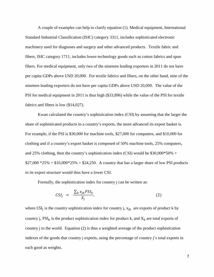
A couple of examples can help to clarify equation (1). Medical equipment, International
Standard Industrial Classification (ISIC) category 3311, includes sophisticated electronic
machinery used for diagnoses and surgery and other advanced products. Textile fabric and
fibers, ISIC category 1711, includes lower-technology goods such as cotton fabrics and spun
fibers. For medical equipment, only two of the nineteen leading exporters in 2011 do not have
per capita GDPs above USD 20,000. For textile fabrics and fibers, on the other hand, nine of the
nineteen leading exporters do not have per capita GDPs above USD 20,000. The value of the
PSI for medical equipment in 2011 is thus high ($33,896) while the value of the PSI for textile
fabrics and fibers is low ($14,027).
Kwan calculated the country’s sophistication index (CSI) by assuming that the larger the
share of sophisticated products in a country’s exports, the more advanced its export basket is.
For example, if the PSI is $30,000 for machine tools, $27,000 for computers, and $10,000 for
clothing and if a country’s export basket is composed of 50% machine tools, 25% computers,
and 25% clothing, then the country’s sophistication index (CSI) would be $30,000*50% +
$27,000 *25% + $10,000*25% = $24,250. A country that has a larger share of low PSI products
in its export structure would thus have a lower CSI.
Formally, the sophistication index for country j can be written as:
𝐶𝐶𝑃𝑃𝐼𝐼𝑗𝑗 = ∑ 𝑥𝑥𝑗𝑗𝑘𝑘𝑃𝑃𝑃𝑃𝐼𝐼𝑘𝑘𝑘𝑘
𝑋𝑋𝑗𝑗, (2)
where CSIj is the country sophistication index for country j, xjk are exports of product k by
country j, PSIk is the product sophistication index for product k, and Xk are total exports of
country j to the world. Equation (2) is thus a weighted average of the product sophistication
indexes of the goods that country j exports, using the percentage of country j’s total exports in
each good as weights.
8
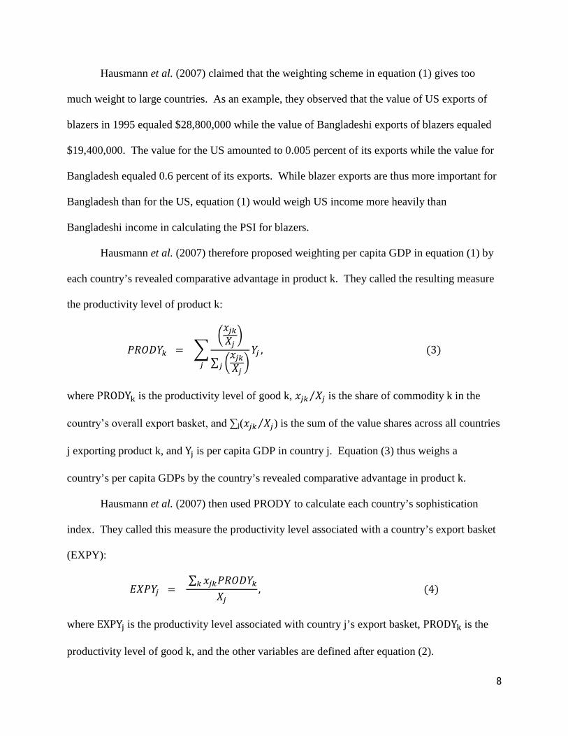
Hausmann et al. (2007) claimed that the weighting scheme in equation (1) gives too
much weight to large countries. As an example, they observed that the value of US exports of
blazers in 1995 equaled $28,800,000 while the value of Bangladeshi exports of blazers equaled
$19,400,000. The value for the US amounted to 0.005 percent of its exports while the value for
Bangladesh equaled 0.6 percent of its exports. While blazer exports are thus more important for
Bangladesh than for the US, equation (1) would weigh US income more heavily than
Bangladeshi income in calculating the PSI for blazers.
Hausmann et al. (2007) therefore proposed weighting per capita GDP in equation (1) by
each country’s revealed comparative advantage in product k. They called the resulting measure
the productivity level of product k:
𝑃𝑃𝑃𝑃𝑃𝑃𝑃𝑃𝑌𝑌𝑘𝑘 = ��𝑥𝑥𝑗𝑗𝑘𝑘𝑋𝑋𝑗𝑗�
∑ �𝑥𝑥𝑗𝑗𝑘𝑘𝑋𝑋𝑗𝑗�𝑗𝑗
𝑌𝑌𝑗𝑗𝑗𝑗
, (3)
where PRODYk is the productivity level of good k, 𝑥𝑥𝑗𝑗𝑘𝑘 𝑋𝑋𝑗𝑗⁄ is the share of commodity k in the
country’s overall export basket, and ∑j(𝑥𝑥𝑗𝑗𝑘𝑘 𝑋𝑋𝑗𝑗⁄ ) is the sum of the value shares across all countries
j exporting product k, and Yj is per capita GDP in country j. Equation (3) thus weighs a
country’s per capita GDPs by the country’s revealed comparative advantage in product k.
Hausmann et al. (2007) then used PRODY to calculate each country’s sophistication
index. They called this measure the productivity level associated with a country’s export basket
(EXPY):
𝐸𝐸𝑋𝑋𝑃𝑃𝑌𝑌𝑗𝑗 = ∑ 𝑥𝑥𝑗𝑗𝑘𝑘𝑃𝑃𝑃𝑃𝑃𝑃𝑃𝑃𝑌𝑌𝑘𝑘𝑘𝑘
𝑋𝑋𝑗𝑗, (4)
where EXPYj is the productivity level associated with country j’s export basket, PRODYk is the
productivity level of good k, and the other variables are defined after equation (2).
9
We use both Kwan’s (2002) approach (equations (1) and (2)) and Hausmann et al’s
(2007) approach (equations (3) and (4)) to measure PSI’s for individual products and CSI’s for
each country’s export basket. Exports are disaggregated at the four-digit ISIC level and are
measured in U.S. dollars for the world’s 89 leading exporters. Per capita GDP is also measured
in (constant) US dollars. These data are obtained from the CEPII-CHELEM database.
We also investigate Switzerland’s export structure using OECD classifications. They
categorize technology levels based on the ratio of R&D spending to value-added (see
Hatzichronoglou, 1997). Their measure provides independent evidence that we can compare
with the results obtained using Kwan’s (2002) and Hausmann et al.’s (2007) techniques.
2.2 Results
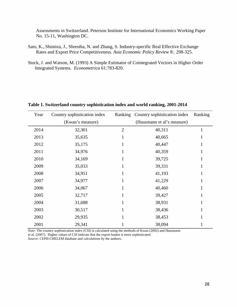
Table 1 presents the results over the 2001-2014 period. Results for earlier years are
available on request. According to Kwan’s (2002) measure Switzerland has the highest country
sophistication index for every year but one in the table. According to Hausmann et al’s (2007)
measure, Switzerland has the highest CSI for every year in the table.
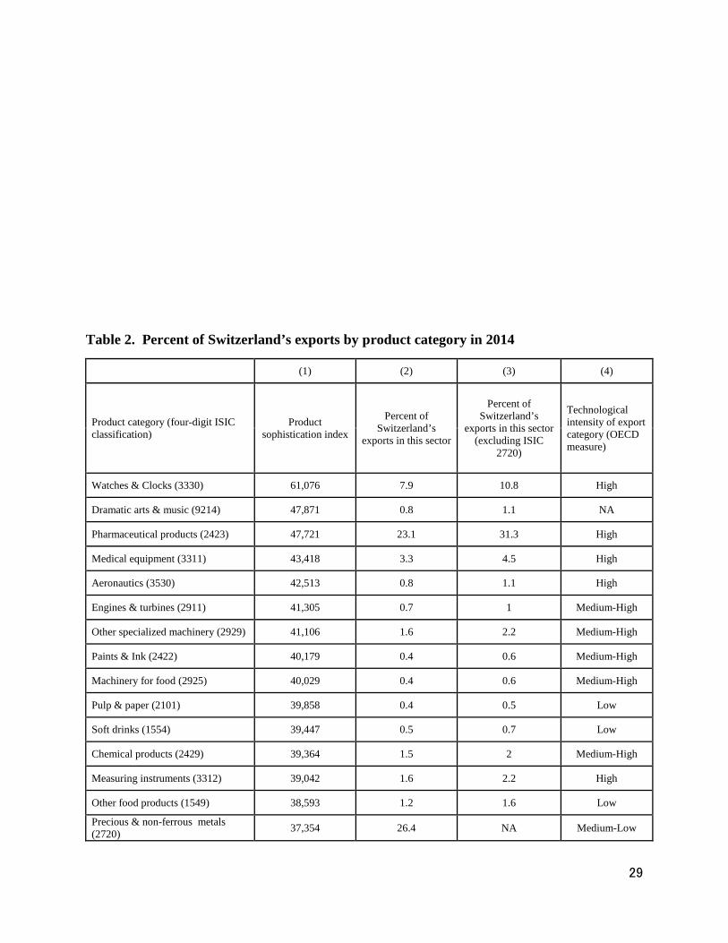
Table 2 presents the percentage of Swiss exports in individual four-digit ISIC categories
in 2014 and the associated product sophistication index calculated using Kwan’s (2002)
methodology. The results are similar when the PSI is calculated using Hausmann et al’s (2007)
approach. We focus on the results in column (3) excluding ISIC category 2720 (precious and
non-ferrous metals). This category averaged 3 percent of Switzerland’s exports from 1989 to
2011 and then jumped to average 32 percent of Swiss exports between 2012 and 2014. Imports
of this category also jumped to average 32 percent of imports between 2012 and 2014. This rise
in imports and exports of precious metals reflects gold bars that are imported, processed in
Switzerland, and then re-exported. Little of the value-added comes from Switzerland. We do
10
not believe that including category 2720 provides an accurate measure of Switzerland’s
industrial structure.
Abstracting from ISIC category 2720, 48% of Swiss exports in 2014 were in categories
with PSI’s above $43,000. For the G-7 countries, the corresponding values were 5% for Canada,
9% for France, 8% for Germany, 7% for Italy, 2% for Japan, 10% for the U.K., and 7% for the
U.S. Column (3) of Table 2 also indicates that 67 percent of Swiss exports were in categories
with PSIs above $35,000. For the G-7 countries, the corresponding values were 9% for Canada,
25% for France, 15% for Germany, 13% for Italy, 11% for Japan, 19% for the U.K., and 13% for
the U.S. The sophistication of Swiss exports is thus an outlier relative to other advanced
economies.
Another way to measure the sophistication of Swiss exports is to examine the percentage
of manufactured exports that are classified by the OECD as high-technology goods. For
Switzerland, abstracting from ISIC category 2720, 53% of exports in 2014 are classified as high-
technology goods based on this criterion. For the G-7 countries, the corresponding share of
high-technology exports was 13% for Canada, 28% for France, 20% for Germany, 11% for Italy,
20% for Japan, 24% for the U.K., and 21% for the U.S.
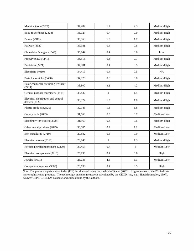
Table 2 indicates that 39% of exports are in ISIC category 24 (chemicals), 18% are in
category 29 (machinery and equipment), and 11% are in category 33 (medical, precision, and
optical instruments). Thus 70% of Swiss exports are from these three advanced industries.
By contrast, traditional lower-technology Swiss products make up a small share of
exports. Chocolates equal only 0.6 percent of exports; cheeses and dairy products only 0.4
percent; wines only 0.04 percent; and fruits only 0.01 percent.
11
Table 2 also indicates that intermediate goods exports such as engines, electronic
components, and parts for vehicles are not large. In total, intermediate goods accounted for 8%
of Swiss exports and 10% of Swiss imports) in 2014. Thus cross-border supply chains are not as
important in Switzerland as they are for East Asian countries, where the share of intermediate
goods in exports and imports often exceeds 30%. In addition, Table 2 indicates that primary
products exports are minuscule. Finally, although not shown in the table, abstracting from ISIC
category 2720 exports, 76 percent of Swiss exports in 2014 went to OECD countries.
Thus Switzerland exports sophisticated products largely to developed economies. One
might expect these to compete on quality more than on price, and thus for the price elasticities of
exports to be small. We investigate this issue in the next section.
3. Estimating export elasticities using time series methods
3.1 Data and Methodology
To estimate trade elasticities we use the workhorse imperfect substitutes model (see
Goldstein and Khan, 1985). Export functions can be written as:
ext = α1 + α2reert + α3yt* + εt , (5)
where ext represents real exports, reert represents the real effective exchange rate, and yt*
represents real foreign income.
We estimate equation (5) using dynamic ordinary least squares (DOLS). DOLS yields
consistent and efficient estimates (Stock and Watson, 1993). The DOLS estimator also has
smaller bias and root mean squared error than other cointegrating regression estimators in cases
where the sample is not large enough to justify applying asymptotic theory (Montalvo, 1995).

12
DOLS estimates of the long run parameters α1, α2, and α3 can be obtained from the following
regression:
)6(,** ,2,1321 t
K
Kkktk
K
Kkktkttt yreeryreerex εββααα +∆+∆+++= ∑∑
−=+
−=+
where K represents the number of leads and lags of the first differenced variables and the other
variables are defined above. We use the Schwarz Criterion to determine the number of leads and
lags.
Equation (5) can also be written in vector error correction form as:
Δext = β10 + φ1(ext-1 – α1 - α2reert-1 - α3yt-1*) + β11(L)Δext-1 +
β12(L)Δ reert-1 + β13(L)Δyt-1* + ν1t (7a)
Δreert = β20 + φ2(ext-1 – α1 - α2reert-1 - α3yt-1*) + β21(L)Δext-1 +
β22(L)Δ reert-1 + β23(L)Δyt-1* + ν2t (7b)
Δyt* = β30 + φ3(ext-1 – α1 - α2reert-1 - α3yt-1*) + β31(L)Δext-1 +
β32(L)Δ reert-1 + Β33(L)Δyt-1* + ν3t . (7c)
φ1, φ2 , and φ3 are error correction coefficients that measure how quickly exports, the real
exchange rate, and income respectively respond to disequilibria. If these endogenous variables
move towards their equilibrium values, the corresponding correction coefficients will be negative
and statistically significant. The L’s represent polynomials in the lag operator. We estimate
equations (7a) – (7c) using Johansen maximum likelihood methods.
Data on the volume of goods exports from Switzerland to the world are available from
the IMF’s International Financial Statistics (IFS) database. Quarterly data are available from
13
1989 to 2016.
CPI-deflated reer data are available from IFS and from the Bank for International
Settlements (BIS). We use both measures.3
For rest of the world income ( ) we use quarterly data on real income in OECD
countries. These data should be useful since the lion’s share of Swiss exports goes to OECD
countries. The data are seasonally adjusted and are obtained from the OECD.4
Augmented Dickey-Fuller tests indicate that the series are integrated of order one. The
trace statistic and the maximum eigenvalue statistic then allow us to reject at the 5% level the
null of no cointegrating relations against the alternative of one cointegrating relation.
3.2 Results
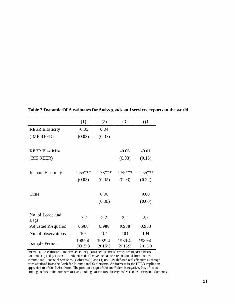
Table 3 presents the results from estimating equation (5). The first row presents the
results using the IMF reer variable and the second row using the BIS reer measure. The first and
third columns present results without a trend and the second and fourth columns present results
with a trend.
The exchange rate elasticities are very small and not statistically significant in any
specification. By contrast, the GDP elasticities are always significant at the 1 percent level and
range from 1.55 to 1.73. The results indicate that a 10 percent increase in rest of the world GDP
would increase exports by 16 to 17 percent.
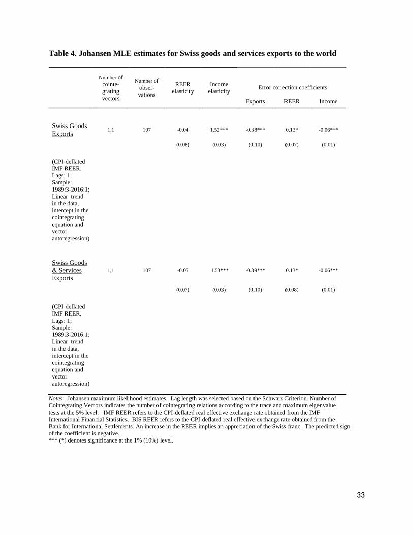
Table 4 provides Johansen maximum likelihood estimates for equations (7a) – (7c) with a
linear trend in the data. The exchange rate elasticities remain close to zero and are not
statistically significant. The GDP elasticites range from 1.52 to 1.53 and are significant at the 1
3 The website for the IMF is www.imf.org. The website for the BIS is www.bis.org. 4 The website for these data is http://stats.oecd.org
*ty
14
percent level. These findings indicate that a 10 percent increase in GDP would increase exports
by 15 percent.
The error correction coefficients for exports are negative and statistically significant,
indicating that exports return to their equilibrium values. The correction coefficients imply that
the gap between the current value of exports and the equilibrium value closes at a rate of 38 or
39 percent per quarter. This implies that 85 percent of the gap between actual and predicted
exports will close within a year. There is thus a tight relationship between exports and the
dependent variables.
The error correction coefficients for the exchange rate is not statistically significant at the
5 percent level. This indicates that this variable is weakly exogenous. The estimated exchange
rate elasticities can thus be interpreted as the response of exports to exogenous changes in reer.
The results reported here indicate that exchange rates do not affect aggregate exports. On
the other hand, there is a strong and very precisely estimated relationship between exports and
real GDP. The findings indicate that a slowdown in the rest of the world would cause a first
order decline in Swiss exports.
4. Estimating export elasticities using panel data
4.1 Data and Methodology
In this section we use the Mark-Sul weighted DOLS estimator to estimate trade
elasticities. We construct panel data sets including Switzerland’s exports to its major importing
countries over the 1989-2014 period. We exclude countries that were minor importers over part
of the sample period because these countries can have large percentage changes in imports due to
idiosyncratic factors rather than due to the macroeconomic variables in equation (5). The major
15
importing countries over the whole sample period are Austria, Belgium Canada, France,
Germany, Hong Kong, Israel, Italy, Japan, Netherlands, Spain, Sweden, the United Kingdom,
and the United States.
We obtain annual data on exports and real GDP from the CEPII-CHELEM database.
Exports are measured in U.S. dollars. We deflate this using the product of the Swiss franc unit
value index and the dollar/CHF exchange rate. These data are obtained from the IMF IFS
database.
We employ the CEPII-CHELEM bilateral real exchange rate between Switzerland and
each of the importing countries. An increase in the exchange rate represents an appreciation of
the exporter’s currency.
We perform a battery of panel unit root tests and Kao (1999) and Pedroni (2004)
cointegration tests on the variables. The results provide some evidence of cointegrating
relations among the variables.
We use Mark and Sul (2003) panel DOLS techniques to find trade elasticities. The
estimated model takes the form:
.,,1;,,1,
)8(
,,
*,,,2,,,1
*,2,10,,
NjTtu
yreryrerex
tji
p
pkktjkj
p
pkktjkjtjtjtji
==
+
∆+∆+++= ∑∑−=
−−=
− ααβββ
Here tjiex ,, represents real exports from Switzerland to country j, tjrer , represents the
bilateral real exchange rate between Switzerland and importing country j, and *
,tjy
represents real income in country j. Cross-section specific lags and leads of the first
differenced regressors are included to asymptotically remove endogeneity and serial
16
correlation.5 A sandwich estimator is employed to allow for heterogeneity in the long-run
residual variances. Individual specific fixed effects and individual specific time trends are
also included.
We also estimate elasticities for individual sectors. Economists since Orcutt (1950) have
recognized the benefits of estimating trade elasticities for individual sectors, since aggregate
estimates of price elasticities may be biased downwards. We investigate the following sectors:
capital goods, consumption goods, non-pharmaceutical products, pharmaceutical product, and
watches. 6 Data on sectoral exports come from the CEPII-CHELEM database and are deflated
using the same measure as before.
4.2 Results
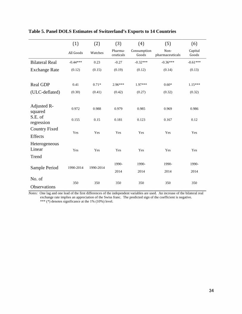
Table 5 present the findings. Column (1) presents the results for all goods and the
subsequent columns are ordered from the industry least affected by exchange rates to the
industry most affected. For all goods the exchange rate coefficient equals -0.44, and is
statistically significant at the 1 percent level. This implies that a 10 percent exchange rate
increase would decrease exports by 4.4 percent. This is very close to Auer and Sauré’s (2012)
findings with disaggregated data that indicated that a 10 percent appreciation would reduce
exports by 4.2 percent. The GDP elasticity is not statistically significant, although it is for
several individual sectors.
5 We employ one lead and one lag. 6 As defined by the CEPII-CHELM database, capital and equipment goods come from the following product categories: aeronautics, agricultural equipment, arms, commercial vehicles, computer equipment, construction equipment, electrical apparatus, electrical equipment, precision instruments, ships, specialized machines, and telecommunications equipment. Consumption goods come from the following categories: beverages, carpets, cars, cereal products, cinematographic equipment, clocks, clothing, consumer electronics, domestic electrical appliances, knitwear, miscellaneous manufactured articles, optics, pharmaceuticals, photographic equipment, preserved fruit and vegetable products, preserved meat and fish products, soaps and perfumes (including chemical preparations), sports equipment, toiletries, toys, and watches.
17
Columns (2) and (3) report results for watches and pharmaceutical products. In both
cases the exchange rate coefficients are not statistically significant, and for watches it is of the
wrong sign. This suggests that the exchange rate does not matter for these sophisticated
industries. In contrast, the GDP elasticity for pharmaceutical goods equals 2.96 and is
significant at the 1 percent level. This indicates that a 1 percent increase in income in importing
countries would increase pharmaceutical exports by 3 percent. This result may reflect the fact
that, as countries become wealthier, they can purchase more cutting edge drugs.
Column (4) reports results for consumption goods. The trade elasticities are both
significant at the 1 percent level. The results indicate that a 10 percent appreciation would
reduce exports by 3 percent and that a 10 percent increase in rest of the world GDP would
increase exports by 20 percent. Column (5) reports results for all exports other than
pharmaceuticals. The exchange rate coefficient is significant at the one percent level. It indicates
that a 10 percent appreciation would reduce non-pharmaceutical exports by 4 percent. The GDP
coefficient is significant at the ten percent level. It indicates that a 10 percent increase in rest of
the world GDP would increase exports by 6 percent.
The contrast between the GDP elasticity for pharmaceuticals and non-pharmaceuticals is
interesting. The elasticity for pharmaceuticals is large (2.96) and highly significant while the
elasticity for non-pharmaceuticals is small (0.6) and marginally significant. The tight link
between exports and aggregate GDP reported in the last section may partly reflect the strong
relationship between pharmaceutical exports and rest of the world GDP. In addition, the weak
link between both pharmaceutical and watch exports and exchange rates may be one reason why
the aggregate exchange rate elasticities reported in the previous section are small.
18
Column (6) reports elasticities for capital and equipment goods exports. The trade
elasticities are both significant at the 1 percent level. The exchange rate coefficient indicates that
a 10 percent appreciation would reduce capital goods exports by 6 percent and the GDP
coefficient indicates that a 10 percent increase in rest of the world GDP would increase exports
by 11.5 percent.
The important implication of these results is that the most sophisticated exports, watches
and pharmaceutical products, are not sensitive to exchange rates. On the other hand Swiss
capital goods exports, which are primarily medium high-technology products, are highly exposed
to appreciations. The recent 30 percent appreciation of the exchange rate thus put significant
downward pressure on capital goods exports.
5. The Pass-Through of Exchange Rate Changes to Export Prices
5.1 Data and Methodology
As Campa and Goldberg (2005) showed, export prices can be represented as the product
of marginal costs and firms’ markup. Employing their framework, Ceglowski (2010) expressed
the first difference of export prices as a function of current and lagged values of the first
difference of the exchange rate, foreign prices, domestic costs, and economic activity in the
destination market:
)9(,
04
03
0 0210 uycpep t
q
i
f
iti
p
iijti
p
i
p
i
f
itiijti
x
jt ∑ ∆∑ ∆∑ ∑ ∆∆∆=
−=
−= =
−−+++++= βββββ
where px
j is the price of exports in industry j, ej
is the exchange rate,
p f
measures foreign
prices, c j represents costs for industry j , and y f
represents economic activity in the export
market.
19
The Swiss franc price of exports by industry (px
j ) is available from the Swiss Federal
Customs Administration. The Swiss franc nominal effective exchange rate (ej ) is available
from the IMF International Financial Statistics database. The foreign price measure (p f
) is
calculated as the geometrically weighted average of the producer price index (PPI) in
Switzerland’s ten leading export destination, and the PPI data are obtained from the CEIC
database. The time-varying weights used to calculatep f
are determined by the share of Swiss
exports going to each of the countries. Costs (c j ) are represented by the PPI in Swiss industry
j, with the data obtained from the Swiss Federal Statistical Office. Economic activity in export
markets (y f
) is measured by a geometrically weighted average of industrial production (IP) in
Switzerland’s ten leading export destination, with the IP data sourced from the IMF
International Financial Statistics database.
To estimate equation (9), we can only use sectors where corresponding data for both
export prices and producer prices are available. We investigate the following sectors: (1) capital
goods, (2) clothing, (3) consumer durables, (4) food, (5) precision instruments, clocks, &
jewelry, and (6) watches & clocks. We also estimate equation (9) for all goods.
Individual sectoral data are available starting in April 2003 and data for all goods are
available starting in April 2000. The sample period for the individual sectors thus extends from
April 2003 to May 2016 and the sample period for all goods extends from April 2000 to May
2016. The estimation begins with six lags of ej
,
p f
, and c j and y f
. To avoid overfitting,
20
the lag length is then progressively reduced by one down to a minimum of two lags and the
Schwarz Criterion is used to choose between the models.
5.2 Results
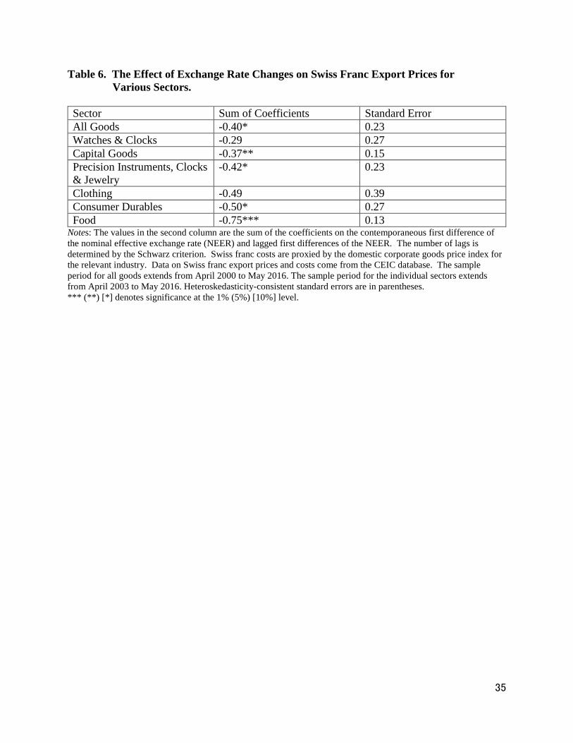
Table 6 reports the sum of the coefficients on the contemporaneous first difference of the
nominal effective exchange rate (ΔNEER) and lagged first differences of the NEER.7 A
negative coefficient implies that an appreciation would lower Swiss franc export prices. The
table presents the findings for all goods first, and the other results are ordered from the industry
where export prices fall the least following an appreciation to the industry where they fall the
most.
The first row reports results for all goods. The coefficient on NEER equals -0.40,
implying that a 10 percent appreciation of the franc would lower Swiss franc export prices by 4.0
percent. The coefficient is statistically significant at the 10 percent level.
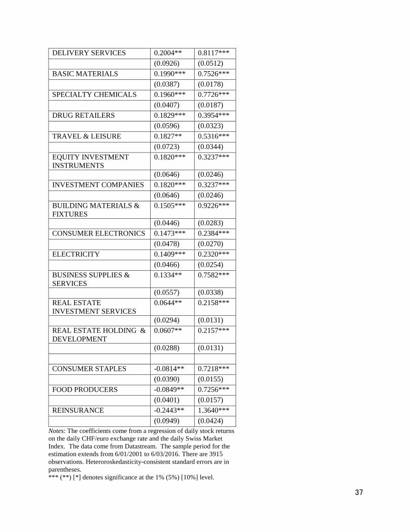
Figure 1 sheds light on the relationship between the exchange rate and export prices for
all goods. It shows that initially as the Swiss franc began appreciating during the GFC, Swiss
franc export prices increased rather than decreased. However, in May 2010 as the Euro Crisis
intensified and the franc appreciation accelerated, export prices tumbled. This fall continued
until the Swiss National Bank set a floor on the exchange rate in the third quarter of 2011. The
figure uses quarterly data, but the relationship is starker using monthly data. From May 2010 to
August 2011, the NEER appreciated logarithmically by 25 percent and export prices fell by 14
percent. This fall in prices squeezed profit margins for Swiss exporters. Then as the SNB
stabilized exchange rates in the third quarter of 2011, export prices began recovering.
7 Results for the other variables are available on request.

21
The second row of Table 6 reports the results for watches and clocks. The coefficient on
NEER equals -0.29, implying that a 10 percent appreciation of the franc would lower export
prices by 2.9 percent. The coefficient is not statistically significant though. These results imply
that an appreciation would have a small effect on average on export prices for watches. One
reason why the coefficient is not more precisely estimated is probably because there is a range of
watches, from high end ones produced by companies such as Rolex to lower end ones made by
companies such as Swatch. Luxury brands may be better able to pass through exchange rate
changes into foreign prices, whereas bargain brands may possess less pricing power.
The third row reports results for capital goods. The coefficient on NEER equals -0.37,
implying that a 10 percent appreciation of the franc would lower export prices by 3.7 percent.
The coefficient is statistically significant. Swiss manufacturing equipment and machine tools are
well-engineered, and do not compete only on price. Nevertheless, the large fall in export prices
during the Eurozone Crisis posed challenges for capital goods makers.
The fourth row presents results for precision instruments, clocks, & jewelry, the fifth row
for clothing, the sixth row for consumer durables, and the seventh for food. The results for
precision instruments are similar to the results for all goods. For consumer durables and food,
the degree of exchange rate pass through is least. For food, for instance, a 10 percent
appreciation will cause a 7.5 percent drop in Swiss franc export prices. Since consumer durables
and especially food tend to be more homogeneous, it is not surprising that firms in these sectors
have limited pricing power.
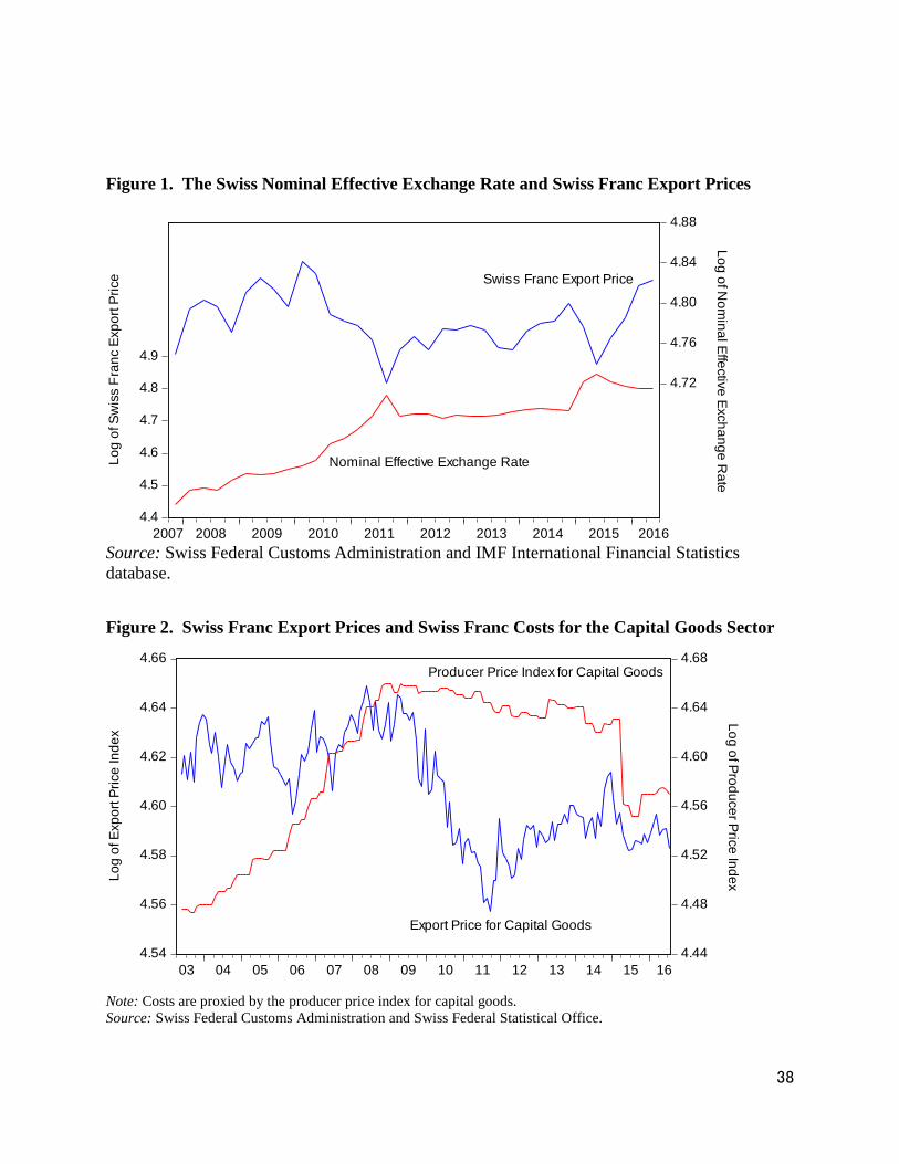
These results indicate that the CHF appreciation lowered Swiss franc export prices.
Figure 2 plots Swiss franc export prices for capital goods and Swiss franc costs as proxied by the
producer price index for capital goods. The figure indicates that prices tumbled relative to costs.
22
The important implication of these results is that the appreciation until 2011Q3 squeezed profit
margins for Swiss companies. To shed further light on this, the next section investigates how
exchange rate changes affect stock returns.
6. The Exchange Rate Exposure of Sectoral Stock Returns
6.1 Data and Methodology
We can investigate how exchange rates affect industry profitability by estimating
exchange rate exposures (see, e.g., Chamberlain, Howe, and Popper, 1997, Dominguez and
Tesar, 2006, or Jayasinghe and Tsui, 2008). This involves regressing industry stock returns
(∆Ri,t ) on exchange rate changes (∆et) and changes in aggregate stock market returns (∆RM,t):
∆Ri,t = αi + βi,e ∆et + βi,M ∆RM,t + εi,t . (7)
We estimate this model for a cross section of industries.
Stock return data are obtained from the Datastream database. Industry stock returns are
calculated as the daily change in the natural log of the industry stock index. The daily change in
the exchange rate is calculated as the daily change in the natural log of the Swiss franc to euro
nominal exchange rate. The variable ∆RM is measured as the daily change in the natural log of
the Swiss Market Index (SMI). The SMI is a value-weighted aggregate index that covers 90
percent of the market capitalization of Swiss companies.
The sample period extends from 1 June 2001 to 3 June 2016. There are 3915
observations.
6.2 Results
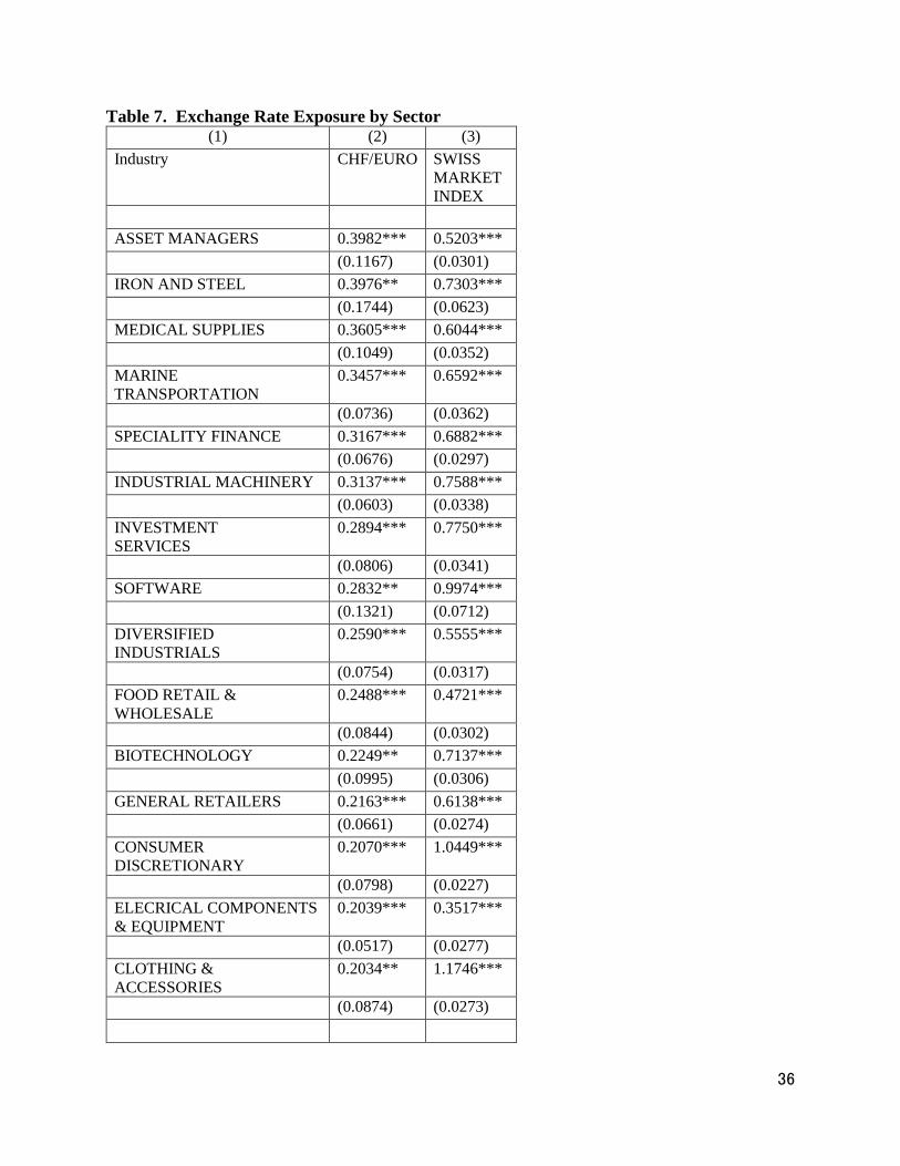
Table 7 presents the results. Only indexes with statistically significant exchange rate
exposures are listed. Column (2) presents the exchange rate exposures and column (3) presents
23
the market exposure. Positive values of the exchange rate exposure in column (2) implies that a
weaker Swiss franc raises stock returns. In other words, the larger the coefficient in column (2),
the more the sector is harmed by an appreciation of the Swiss franc.
The results indicate that the financial services industry is heavily exposed to a CHF
appreciation. Seven categories of financial services have statistically significant exposures.
Listed from the most exposed to the least exposed, these are: asset managers, specialty finance,
investment services, equity investment instruments, investment companies, real estate investment
services, and real estate holding & development. Across all industries, the category asset
managers is the most exposed and the category specialty finance is the fifth most exposed. For
asset managers, the results indicate that a 1 percent depreciation of the Swiss franc would
increase returns by 0.40 percent and for specialty finance the results indicate that a 1 percent
depreciation of the franc would raise returns by 0.32 percent.
The retail sector is also exposed to an appreciation of the Swiss franc. Food retailers &
wholesalers, general retailers, and drug retailers all have statistically significant exposures. For
food retailers & wholesalers, a 1 percent depreciation of the Swiss franc would increase returns
by 0.25 percent. The exposure of retailers could reflect the fact that many customers can respond
to an appreciation of the franc by going to neighboring countries and buying goods in euros.
Industrial machinery and diversified industrial stocks are also among the most harmed by
an appreciation. This could reflect the findings in the previous section indicating that a CHF
appreciation squeezed the profit margins of sectors such as capital good. The results indicate
that a 1 percent Swiss franc depreciation would increase returns on industrial machinery by 0.31
percent.
24
We can also learn from the industries that are not listed in Table 7 and thus do not have a
statistically significant exposure to exchange rate changes. One of these is the pharmaceutical
sector. Being so research-intensive and sophisticated, it may be able to maintain profit margins
in response to an appreciation of the Swiss franc. Another is specialty retail. Stores selling
specialized goods such as Swiss army knives may be less exposed to customers going to
neighboring countries to buy goods.
Table 7 also indicate that food producers and reinsurance companies benefit from CHF
appreciations. For food producers, this may reflect the fact that appreciations reduce the prices
of imported inputs. For instance, the cost of imported cocoa beans will fall as the CHF
appreciates. For reinsurance companies, this may reflect an imbalance between assets and
liabilities such that a stronger franc increases their net worth.
7. Conclusion
Switzerland produces sophisticated products, runs budget surpluses, maintains low
inflation, possesses a strong currency, and excels at wealth management. These factors make it
attractive to investors in times of turmoil, and has led to safe haven capital inflow and CHF
appreciations since the Global Financial Crisis. This paper investigates how exchange rates
affect the Swiss economy.
The results indicate that Swiss exports are very sensitive to rest of the world GDP. In
addition, companies exporting high-end watches and research-intensive pharmaceutical products
are able to weather appreciations well. However, companies exporting medium-high-technology
capital goods face shocks to profitability and export volume when the Swiss franc soars.
25
Several policy lessons flow from the findings reported here. First, the results indicate
that there is a tight relationship between Swiss exports and rest of the world GDP. The Swiss
economy is dependent on exports because of its small domestic market. Therefore Switzerland
has a strong interest in the economic welfare of its trading partners. It should foster this by, for
instance, maintaining free trade and scientific exchanges with developed countries and by
sharing its expertise in areas such as healthcare and education with developing economies.
Second, the findings indicate that the most advanced industries can maintain their exports
and their profitability in the face of exchange rate appreciations while medium-high- technology
industries suffer tumbling exports and stock prices. Japan, like Switzerland, experienced safe
haven capital inflows and exchange rate appreciations during the GFC. Japan’s export structure
contains fewer high-technology products and more medium high-technology products than
Switzerland’s does. The Japanese electronics sector, once the flagship of its economy, was
devastated by the strong yen after 2007 (see, e.g., Sato et al., 2013). The results here suggest
that if Japan could upgrade its industrial structure to include more high-technology goods, it
would be better able to handle the appreciations that accompany safe haven inflows. Japan does
not necessarily need to upgrade to the same goods that Switzerland produces, but rather produce
advanced goods that are consistent with Japan’s comparative advantage.
Finally, if the exchange rate is so important for Switzerland’s economy, how much more
important it must be for economies exporting labor-intensive goods and other lower-technology
products. Politicians in each country thus have a strong incentive to pursue stealth devaluations
to gain a larger share of limited world demand.8 This will likely lead to currency wars.
8 Rodrik (2008) reported that exchange-rate undervaluations increase economic growth. He found that exchange-rate undervaluations raise the share of the tradeable sector in total output. He then reported that the tradeable sector in developing countries tends to be inefficiently small because of government or market failures. He thus concludes that an undervalued exchange rate that increases the size of the tradeable sector will stimulate growth.
26
Economists should focus on how to reform the international monetary system to encourage
policymakers to pursue longer-run cosmopolitan interests rather than short-run nationalistic
agendas.
REFERENCES
Arbatli, E., and Hong, G. H. (2016) Singapore’s Export Elasticities: A Disaggregated Look into the Role of Global Value Chains and Economic Complexity. International Monetary Fund Working Paper No. 16-52, Washington DC.
Auer, R. and Sauré, P. (2011) Export Basket and the Effects of Exchange Rates on Export – Why
Switzerland Is Special. Federal Reserve Bank of Dallas, Globalization and Monetary Policy Institute Working Paper No. 77, Dallas, Texas.
Auer, R. and Sauré, P. (2012) CHF Strength and Swiss Export Performance – Evidence and
Outlook from a Disaggregated Analysis. Applied Economics Letters 19: 521-531. Campa, J., Goldberg, L. (2005) Exchange rate pass-through into import prices. The Review of
Economics and Statistics 87: 679-690. Ceglowski, J. (2010) Has pass-through to export prices risen? Evidence for Japan. Journal of the
Japanese and International Economies 24: 86-98. Chamberlain, S., Howe, J. S. and Popper, H. (1997) The Exchange Rate Exposure of U. S. and
Japanese Banking Institutions. Journal of Banking and Finance 21: 871-892. Dominguez, K. M. E., and Tesar, L. L. (2006) Exchange Rate Exposure. Journal of International
Economics 68: 188-218. Goldstein, M. and Khan, M. (1985) Income and Price Effects in Foreign Trade. Handbook of
International Economics (R. Jones, and P. P. Kenen, Eds.). Amsterdam Elsevier. Héricourt, J., Martin, P. and Orefice, G. (2014). Les exportateurs français face aux variations de l’euro. La Lettre du CEPII 340. Centre D’Etudes Prospectives et D’Information Internationales. Hatzichronoglou, T. (1997) Revision of the High-Technology Sector and Product Classification. OECD Science, Technology and Industry Working Paper No. 1997-02, Paris. Hausmann, R., Hwang, J. and Rodrik, D. (2007) What You Export Matters. Journal of Economic Growth 12:1-25.
27
Hidalgo, C. A., and Hausmann, R., (2009) The Building Blocks of Economic Complexity. Harvard University Mimeo. Available at: https://arxiv.org/ftp/arxiv/papers/0909/0909.3890.pdf.
International Monetary Fund (2013) Switzerland: Selected Issues Paper. IMF Country Report, No 13-129. Available at: http://www.imf.org/external/pubs/ft/scr/2013/cr13129.pdf. International Monetary Fund (2011) Switzerland: Selected Issues Paper. IMF Country Report, No 11-116. Available at: https://www.imf.org/external/pubs/ft/scr/2011/cr11116.pdf Jayasinghe, P. and Tsui, A. K. (2008) Exchange Rate Exposure of Sectoral Returns and Volatilities: Evidence from Japanese Industrial Sectors. Japan and the World Economy 20: 639-660. Kao, C. (1999) Spurious Regression and Residual-Based Tests for Cointegrated Regression in Panel Data. Journal of Econometrics 90: 1-44 Kwan, C. H. (2002) The Rise of China and Asia’s Flying Geese Pattern of Economic Development: An Empirical Analysis Based on US Import Statistics. Research Institute of Economy, Trade, and Industry Discussion Paper No. 02-E-009, Tokyo. Lall, S., Weiss, J. and Zhang, J. (2006) The "Sophistication" of Exports: A New Trade Measure. World Development 21: 153-172. Mark, N., and Sul, D. (2003) Cointegration Vector Estimation by Panel DOLS and Long‐run Money Demand. Oxford Bulletin of Economics and Statistics 65: 655-680. Montalvo, J. (1995) Comparing Cointegrating Regression Estimators: Some additional Monte Carlo evidence. Economics Letters 48: 229-234. Orcutt, G. (1950) Measurement of Price Elasticities in International Trade, Review of Economics and Statistics 32: 117-132. Pesaran, M. H. and Smith, R.P. (1995) Estimating Long-Run Relationships from Dynamic
Heterogeneous Panels. Journal of Econometrics 68: 79-113.
Pedroni, P. (2004) Panel Cointegration; Asymptotic and Finite Sample Properties of Pooled Time Series Tests with an Application to the Purchasing Power Parity Hypothesis. Econometric Theory 20: 597-625. Rodrik, D. (2008) The Real Exchange Rate and Economic Growth. Brookings Papers on Economic Activity 39: 365-412. Sauré, P. (2015) The Resilient Trade Surplus, the Pharmaceutical Sector, and Exchange Rate
28
Assessments in Switzerland. Peterson Institute for International Economics Working Paper No. 15-11, Washington DC. Sato, K., Shimizu, J., Shrestha, N. and Zhang, S. Industry-specific Real Effective Exchange Rates and Export Price Competitiveness. Asia Economic Policy Review 8:. 298-325. Stock, J. and Watson, M. (1993) A Simple Estimator of Cointegrated Vectors in Higher Order Integrated Systems. Econometrica 61:783-820.
Table 1. Switzerland country sophistication index and world ranking, 2001-2014
Year Country sophistication index Ranking Country sophistication index Ranking (Kwan’s measure) (Hausmann et al’s measure)
2014 32,301 2 40,311 1 2013 35,635 1 40,665 1 2012 35,175 1 40,447 1 2011 34,976 1 40,359 1 2010 34,169 1 39,725 1 2009 35,033 1 39,331 1 2008 34,951 1 41,193 1 2007 34,977 1 41,229 1 2006 34,067 1 40,460 1 2005 32,717 1 39,427 1 2004 31,688 1 38,931 1 2003 30,517 1 38,436 1 2002 29,935 1 38,453 1 2001 29,341 1 38,094 1
Note: The country sophistication index (CSI) is calculated using the methods of Kwan (2002) and Hausmann et al. (2007). Higher values of CSI indicate that the export basket is more sophisticated. Source: CEPII-CHELEM database and calculations by the authors.
29
Table 2. Percent of Switzerland’s exports by product category in 2014
(1) (2) (3) (4)
Product category (four-digit ISIC classification)
Product sophistication index
Percent of Switzerland’s
exports in this sector
Percent of Switzerland’s
exports in this sector (excluding ISIC
2720)
Technological intensity of export category (OECD measure)
Watches & Clocks (3330) 61,076 7.9 10.8 High
Dramatic arts & music (9214) 47,871 0.8 1.1 NA
Pharmaceutical products (2423) 47,721 23.1 31.3 High
Medical equipment (3311) 43,418 3.3 4.5 High
Aeronautics (3530) 42,513 0.8 1.1 High
Engines & turbines (2911) 41,305 0.7 1 Medium-High
Other specialized machinery (2929) 41,106 1.6 2.2 Medium-High
Paints & Ink (2422) 40,179 0.4 0.6 Medium-High
Machinery for food (2925) 40,029 0.4 0.6 Medium-High
Pulp & paper (2101) 39,858 0.4 0.5 Low
Soft drinks (1554) 39,447 0.5 0.7 Low
Chemical products (2429) 39,364 1.5 2 Medium-High
Measuring instruments (3312) 39,042 1.6 2.2 High
Other food products (1549) 38,593 1.2 1.6 Low
Precious & non-ferrous metals (2720) 37,354 26.4 NA Medium-Low
30
Machine tools (2922) 37,282 1.7 2.3 Medium-High
Soap & perfumes (2424) 36,127 0.7 0.9 Medium-High
Pumps (2912) 36,069 1.3 1.7 Medium-High
Railway (3520) 35,981 0.4 0.6 Medium-High
Chocolates & sugar (1543) 35,744 0.4 0.6 Low
Primary plastic (2413) 35,313 0.6 0.7 Medium-High
Pesticides (2421) 34,981 0.4 0.5 Medium-High
Electricity (4010) 34,419 0.4 0.5 NA
Parts for vehicles (3430) 34,378 0.6 0.8 Medium-High
Basic chemicals excluding fertilizer (2411) 33,800 3.1 4.2 Medium-High
General purpose machinery (2919) 33,437 1 1.4 Medium-High
Electrical distribution and control devices (3120) 33,322 1.3 1.8 Medium-High
Plastic products (2520) 32,143 1.3 1.8 Medium-High
Cutlery tools (2893) 31,663 0.5 0.7 Medium-Low
Machinery for textiles (2926) 31,569 0.4 0.6 Medium-High
Other metal products (2899) 30,005 0.9 1.2 Medium-Low
Iron metallurgy (2710) 29,882 0.6 0.9 Medium-Low
Electrical motors (3110) 29,746 1 1.3 Medium-High
Refined petroleum products (2320) 29,453 0.7 1 Medium-Low
Electrical components (3210) 26,938 0.4 0.6 High
Jewelry (3691) 26,735 4.5 6.1 Medium-Low
Computer equipment (3000) 20,630 0.4 0.5 High
Note: The product sophistication index (PSI) is calculated using the method of Kwan (2002). Higher values of the PSI indicate more sophisticated products. The technology intensity measure is calculated by the OECD (see, e.g., Hatzichronoglou, 1997). Source: CEPII-CHELEM database and calculations by the authors.
31
Table 3 Dynamic OLS estimates for Swiss goods and services exports to the world
(1) (2) (3) ()4
REER Elasticity -0.05 0.04 (IMF REER) (0.08) (0.07)
REER Elasticity -0.06 -0.01 (BIS REER) (0.08) (0.16)
Income Elasticity 1.55*** 1.73*** 1.55*** 1.66***
(0.03) (0.32) (0.03) (0.32)
Time 0.00 0.00
(0.00) (0.00)
No. of Leads and Lags 2,2 2,2 2,2 2,2
Adjusted R-squared 0.988 0.988 0.988 0.988 No. of observations 104 104 104 104
Sample Period 1989:4-2015:3
1989:4-2015:3
1989:4-2015:3
1989:4-2015:3
Notes: DOLS estimates. Heteroskedasticity-consistent standard errors are in parentheses. Columns (1) and (2) use CPI-deflated real effective exchange rates obtained from the IMF International Financial Statistics. Columns (3) and (4) use CPI-deflated real effective exchange
rates obtained from the Bank for International Settlements. An increase in the REER implies an appreciation of the Swiss franc. The predicted sign of the coefficient is negative. No. of leads and lags refers to the numbers of leads and lags of the first differenced variables. Seasonal dummies
32
are included in the regressions. *** denotes significance at the 1% level.
33
Table 4. Johansen MLE estimates for Swiss goods and services exports to the world
Number of
cointe-grating vectors
Number of obser-vations
REER elasticity
Income elasticity
Error correction coefficients
Exports REER Income
Swiss Goods Exports 1,1 107 -0.04 1.52*** -0.38*** 0.13* -0.06***
(0.08) (0.03) (0.10) (0.07) (0.01)
(CPI-deflated IMF REER. Lags: 1; Sample: 1989:3-2016:1; Linear trend in the data, intercept in the cointegrating equation and vector autoregression)
Swiss Goods & Services Exports
1,1 107 -0.05 1.53*** -0.39*** 0.13* -0.06***
(0.07) (0.03) (0.10) (0.08) (0.01)
(CPI-deflated IMF REER. Lags: 1; Sample: 1989:3-2016:1; Linear trend in the data, intercept in the cointegrating equation and vector autoregression)
Notes: Johansen maximum likelihood estimates. Lag length was selected based on the Schwarz Criterion. Number of Cointegrating Vectors indicates the number of cointegrating relations according to the trace and maximum eigenvalue tests at the 5% level. IMF REER refers to the CPI-deflated real effective exchange rate obtained from the IMF International Financial Statistics. BIS REER refers to the CPI-deflated real effective exchange rate obtained from the Bank for International Settlements. An increase in the REER implies an appreciation of the Swiss franc. The predicted sign of the coefficient is negative. *** (*) denotes significance at the 1% (10%) level.
34
Table 5. Panel DOLS Estimates of Switzerland’s Exports to 14 Countries
(1) (2) (3) (4) (5) (6)
All Goods Watches Pharma-ceuticals
Consumption Goods
Non-pharmaceuticals
Capital Goods
Bilateral Real -0.44*** 0.23 -0.27 -0.32*** -0.36*** -0.61***
Exchange Rate (0.12) (0.15) (0.19) (0.12) (0.14) (0.13)
Real GDP 0.41 0.71* 2.96*** 1.97*** 0.60* 1.15***
(ULC-deflated) (0.30) (0.41) (0.42) (0.27) (0.32) (0.32)
Adjusted R-squared 0.972 0.988 0.979 0.985 0.969 0.986
S.E. of regression 0.155 0.15 0.181 0.123 0.167 0.12
Country Fixed Yes Yes Yes Yes Yes Yes
Effects Heterogeneous Linear Yes Yes Yes Yes Yes Yes
Trend
Sample Period 1990-2014 1990-2014 1990- 1990- 1990- 1990-
2014 2014 2014 2014
No. of 350 350 350 350 350 350
Observations Notes: One lag and one lead of the first differences of the independent variables are used. An increase of the bilateral real exchange rate implies an appreciation of the Swiss franc. The predicted sign of the coefficient is negative. *** (*) denotes significance at the 1% (10%) level.
35
Table 6. The Effect of Exchange Rate Changes on Swiss Franc Export Prices for Various Sectors.
Sector Sum of Coefficients Standard Error All Goods -0.40* 0.23 Watches & Clocks -0.29 0.27 Capital Goods -0.37** 0.15 Precision Instruments, Clocks & Jewelry
-0.42* 0.23
Clothing -0.49 0.39 Consumer Durables -0.50* 0.27 Food -0.75*** 0.13
Notes: The values in the second column are the sum of the coefficients on the contemporaneous first difference of the nominal effective exchange rate (NEER) and lagged first differences of the NEER. The number of lags is determined by the Schwarz criterion. Swiss franc costs are proxied by the domestic corporate goods price index for the relevant industry. Data on Swiss franc export prices and costs come from the CEIC database. The sample period for all goods extends from April 2000 to May 2016. The sample period for the individual sectors extends from April 2003 to May 2016. Heteroskedasticity-consistent standard errors are in parentheses. *** (**) [*] denotes significance at the 1% (5%) [10%] level.
36
Table 7. Exchange Rate Exposure by Sector (1) (2) (3)
Industry CHF/EURO SWISS MARKET INDEX
ASSET MANAGERS 0.3982*** 0.5203***
(0.1167) (0.0301) IRON AND STEEL 0.3976** 0.7303***
(0.1744) (0.0623) MEDICAL SUPPLIES 0.3605*** 0.6044***
(0.1049) (0.0352) MARINE TRANSPORTATION
0.3457*** 0.6592***
(0.0736) (0.0362) SPECIALITY FINANCE 0.3167*** 0.6882***
(0.0676) (0.0297) INDUSTRIAL MACHINERY 0.3137*** 0.7588***
(0.0603) (0.0338) INVESTMENT SERVICES
0.2894*** 0.7750***
(0.0806) (0.0341) SOFTWARE 0.2832** 0.9974***
(0.1321) (0.0712) DIVERSIFIED INDUSTRIALS
0.2590*** 0.5555***
(0.0754) (0.0317) FOOD RETAIL & WHOLESALE
0.2488*** 0.4721***
(0.0844) (0.0302) BIOTECHNOLOGY 0.2249** 0.7137***
(0.0995) (0.0306) GENERAL RETAILERS 0.2163*** 0.6138***
(0.0661) (0.0274) CONSUMER DISCRETIONARY
0.2070*** 1.0449***
(0.0798) (0.0227) ELECRICAL COMPONENTS & EQUIPMENT
0.2039*** 0.3517***
(0.0517) (0.0277) CLOTHING & ACCESSORIES
0.2034** 1.1746***
(0.0874) (0.0273)
37
DELIVERY SERVICES 0.2004** 0.8117*** (0.0926) (0.0512)
BASIC MATERIALS 0.1990*** 0.7526*** (0.0387) (0.0178)
SPECIALTY CHEMICALS 0.1960*** 0.7726*** (0.0407) (0.0187)
DRUG RETAILERS 0.1829*** 0.3954*** (0.0596) (0.0323)
TRAVEL & LEISURE 0.1827** 0.5316*** (0.0723) (0.0344)
EQUITY INVESTMENT INSTRUMENTS
0.1820*** 0.3237***
(0.0646) (0.0246) INVESTMENT COMPANIES 0.1820*** 0.3237***
(0.0646) (0.0246) BUILDING MATERIALS & FIXTURES
0.1505*** 0.9226***
(0.0446) (0.0283) CONSUMER ELECTRONICS 0.1473*** 0.2384***
(0.0478) (0.0270) ELECTRICITY 0.1409*** 0.2320***
(0.0466) (0.0254) BUSINESS SUPPLIES & SERVICES
0.1334** 0.7582***
(0.0557) (0.0338) REAL ESTATE INVESTMENT SERVICES
0.0644** 0.2158***
(0.0294) (0.0131) REAL ESTATE HOLDING & DEVELOPMENT
0.0607** 0.2157***
(0.0288) (0.0131)
CONSUMER STAPLES -0.0814** 0.7218*** (0.0390) (0.0155)
FOOD PRODUCERS -0.0849** 0.7256*** (0.0401) (0.0157)
REINSURANCE -0.2443** 1.3640*** (0.0949) (0.0424)
Notes: The coefficients come from a regression of daily stock returns on the daily CHF/euro exchange rate and the daily Swiss Market Index. The data come from Datastream. The sample period for the estimation extends from 6/01/2001 to 6/03/2016. There are 3915 observations. Heteroroskedasticity-consistent standard errors are in parentheses. *** (**) [*] denotes significance at the 1% (5%) [10%] level.
38
Figure 1. The Swiss Nominal Effective Exchange Rate and Swiss Franc Export Prices
4.4
4.5
4.6
4.7
4.8
4.9
4.72
4.76
4.80
4.84
4.88
2007 2008 2009 2010 2011 2012 2013 2014 2015 2016
Nominal Effective Exchange Rate
Swiss Franc Export Price
Log of Nom
inal Effective Exchange Rate
Log
of S
wis
s Fr
anc
Expo
rt Pr
ice
Source: Swiss Federal Customs Administration and IMF International Financial Statistics database.
Figure 2. Swiss Franc Export Prices and Swiss Franc Costs for the Capital Goods Sector
4.54
4.56
4.58
4.60
4.62
4.64
4.66
4.44
4.48
4.52
4.56
4.60
4.64
4.68
03 04 05 06 07 08 09 10 11 12 13 14 15 16
Export Price for Capital Goods
Producer Price Index for Capital Goods
Log
of E
xpor
t Pric
e In
dex
Log of Producer Price Index
Note: Costs are proxied by the producer price index for capital goods. Source: Swiss Federal Customs Administration and Swiss Federal Statistical Office.