Embed Size (px)
Citation preview
Executive equity comepnsation and earnings management:
A quantile regression analysis
Chih-Ying Chen School of Accountancy
Singapore Management University E-mail: [email protected]
Phone: (+65) 68280987 Fax: (+65) 68280600
Ming-Yuan Li Department of Accounting
National Cheng-Kung University Tainan, Taiwan
E-mail: [email protected]: (+886) 6-2757575 ext. 53421
Fax: (+886) 6-2744104
Executive equity comepnsation and earnings management:
A quantile regression analysis
Abstract
Prior research has investigated the association between executive equity compensation and earnings management but the evidence is not conclusive. We investigate this question using the quantile regression approach which allows the coefficient on the independent variable (equity compensation) to shift across the distribution of the dependent variable (earnings management). Based on a sample of 18,203 U.S. non-financial firm-year observations from 1995 to 2008, we find that chief executive officer (CEO) equity compensation is positively associated with the absolute value of discretionary accruals at all quantiles of absolute discretionary accruals, but the association becomes weaker as the quantile decreases. The association between CEO equity compensation and signed values of discretionary accruals is positive (negative) when the discretionary accruals are at the high (medium and low) quantiles. The results are robust to alternative measures of equity incentives and earnings management and alternative model specifications. Overall, the quantile regression results suggest that equity compensation motivates income-increasing earnings management when the firm has low financial reporting quality, but mitigates income-increasing earnings management when the financial reporting quality is high. The results also demonstrate that the least-squares and least-sum optimization techniques which are used commonly in prior research do not capture the behavior of firms at the high and low quantiles of financial reporting quality. Keywords: Equity incentives, executive compensation, quantile regression, earnings
management, discretionary accruals JEL classification: G12; G32 Data Availability: All data are obtained from publicly available sources.
1. Introduction
Whether equity compensation motivates corporate executives to manage
earnings has been debated for years. Academic research also has investigated this
question but the evidence is not conclusive. Most studies find a positive association
between the chief executive officer (CEO) equity compensation and earnings
management, using proxies such as discretionary accruals and restatement of financial
report, but some others do not find a positive association. These different results are
obtained despite that the studies use similar proxies for equity incentives and earnings
management. However, research design could be a factor that causes the different
results. It is common in prior studies on equity compensation and earnings
management to use a matched-pairs sample where a restating firm is matched with a
non-restating firm using a small number of variables such as firm size and industry
classification. Instead of using this common approach, Armstrong et al. (2009) use a
propensity score matching process and find some evidence that the level of CEO
equity incentives has a modest negative relationship with the incidence of accounting
irregularities.
Our study adds to the research on CEO equity compensation and earnings
management by investigating their relationship across the entire distribution of
earnings management using the quantile regression, which does not require the
regression coefficients to be constant. In empirical research, the constant-coefficient
regression models, such as the ordinary least squared (OLS) and least-sum of absolute
deviations (LAD), are used extensively. However, these models only describe the
average behavior of the dependent variable (i.e., central distribution tendency) and the
resulting coefficient estimates are not necessarily indicative of the size and nature of
the effects of the independent variables on the tails of the dependent variable’s
1
distribution. In addition, the analytical framework in prior research tends to assume an
unconditional distribution of firm observations. This form of “sample truncation” may
yield invalid empirical results (Heckman, 1979).
The quantile regression (hereafter, QR) approach was developed by Koenker
and Basset (1978) and used widely in recent economics and finance research.
Quantile describes a division of observations into intervals based on the values of the
data. The QR model is a random-coefficient model in which the parameter of the
independent variable can be expressed as a monotonic function of a single scalar
random variable, hence capturing the systematic influences of the independent
variables on the location, scale, and shape of the conditional distribution of the
dependent variable. The QR approach can be used to examine whether the traditional
optimization techniques fail to address the behaviors in the tail regions of the
dependent variable’s distribution (e.g., at the 0.05 or 0.95 quantile).1 This approach
differs from segmenting the dependent variable into subsets according to its
unconditional distribution and then doing least squares fitting on these subsets. To the
extent that the sample segmentation and the relation between equity compensation
and earnings management are jointly determined, using QR can address the potential
problem in prior studies that assume segmentation of the sample is exogeneous.
We use discretionary accruals as a proxy for earnings management, where
positive (negative) values imply income-increasing (income-decreasing) earnings
management and larger absolute values imply more extreme earnings management.
We measure equity compensation as the fair value of stock options and restricted
stock granted to the CEO scaled by the CEO’s total compensation. The sample
1 As discussed below, the QR model minimizes a sum of weighted absolute residuals. For example, the results at the 0.90 quantile are estimated when the positive (negative) residuals are given a 90 (10) percent of weight. The LAD results are the same as the QR results at the 0.50 quantile where the positive and negative residuals are equally weighted.
2
consists of 18,203 observations of U.S. non-financial firms (S&P 500 and medium
and small cap) for the period from 1995 to 2008. We perform the QR at 19 quantiles,
starting from quantile 0.05 and increasing by 0.05 each time up to quantile 0.95.
In the OLS regression of absolute discretionary accruals, we find the
coefficient on equity compensation to be significantly positive. The QR results also
show a significantly positive coefficient on equity compensation at all quantiles of
absolute discretionary accruals, but the coefficient decreases monotonically as the
quantile decreases, and becomes very small at the low quantiles. The coefficients at
any two adjoining quantiles are significantly different from each other, indicating that
the relation between equity compensation and earnings management varies with the
likelihood of earnings management.
In the OLS regression of signed values of discretionary accruals, we find the
coefficient on equity compensation to be statistically insignificant. However, the QR
results show that the coefficient on equity compensation increases monotonically as
the quantile of signed values of discretionary accruals increases. The coefficient is
significantly negative at the 0.05 to 0.65 quantiles, statistically insignificant at the
0.70 to 0.80 quantiles, and significantly positive at the 0.85 to 0.95 quantiles.
Taken together, the QR results show that equity compensation is positively
associated with absolute and signed values of discretionary accruals only at the high
quantiles of these two accruals measures (i.e. low financial reporting quality). At the
medium and low quantiles of signed values of discretionary accruals, equity
compensation is negatively associated with discretionary accruals. The results are
robust to alternative measures of discretionary accruals and equity incentives (such as
lagged equity compensation to total compensation, and pay-for-performance
sensitivity) and alternative model specifications. Overall, the results suggest that
3
equity compensation motivates income-increasing earnings management in firms with
characteristics associated with lower financial reporting quality. Conversely, in firms
with high financial reporting quality, equity compensation mitigates income-
increasing earnings management. The results also demonstrate that the least-squares
and least-sum optimization techniques used commonly in prior research do not
capture the behavior of firms at the extreme quantiles of financial reporting quality.
Our study contributes to the literature in several ways. First, we employ a
methodology that recognizes heterogeneity in the dependent variable of the regression
(earnings management) and considers the entire distribution of the variable, hence
producing results that cannot be observed under the OLS and LAD approaches.
Second, we use an empirical model that produces quantile-varying estimators rather
than relying on a single measure of conditional central tendency, thereby linking
equity compensation and earnings management in a continuous and smooth manner.
Taking advantage of the less restrictive research design and empirical model, our
study provides evidence that helps to explain the inconsistent findings in prior
research concerning the relationship between CEO equity compensation and earnings
management.
The rest of the paper proceeds as follows. Section 2 reviews related studies
and develops the research questions. Section 3 discusses the theoretical models.
Section 4 describes the sample, variables, and empirical model. Section 5 discusses
the empirical results. Section 6 discusses the results for robustness tests and
alternative specifications. Section 7 summarizes and concludes the paper.
2. Related Studies and research questions
2.1 Studies on equity compensation and earnings management
4
Prior studies have investigated the association between CEO equity
compensation and earnings management extensively. Most studies find positive
associations. For example, Larcker, Richardson, and Tuna (2007) find a positive
association between compensation mix (equity compensation divided by total
compensation) and discretionary accruals, and Bergstresser and Philippon (2006) find
a positive association between incentive ratio and discretionary accruals. Some
studies, however, do not find a statistically significant association between equity
compensation and earnings management (Erickson, Hanlon, and Maydew 2006;
Baber, Kang, and Liang 2007). There is also research showing that the association is
negative. Armstrong, Jagolinzer, and Larcker (2010) find some evidence that
accounting irregularities occur less frequently at firms where CEOs have relatively
higher levels of equity incentives.
Some studies further investigate the association between the components of
equity compensation and earnings management. Harris and Bromiley (2007), Burns
and Kedia (2006), and Efendi, Srivastava, and Swanson (2007), find positive
associations only for option-related compensation, Cheng and Warfield (2005) find
positive associations for unvested options and stock ownership, and Johnson, Ryan,
and Tian (2009) find positive associations for vested stock holdings. O’Connor et al.
(2006) find that the association is positive for option-related equity components only
when conditioned on the board of directors’ composition and compensation structure.
2.2 Development of research questions
Our study differs from prior research on the association between equity
compensation and earnings management in that our analysis incorporates the potential
influences of financial reporting quality on the association. Prior studies document a
link between corporate governance and financial reporting quality (e.g., Dechow et al.
5
1996; Beasley 1996; Klein 2002), and a link between corporate governance and
executive compensation (e.g., Core, Holthausen, and Larcker 1999). Therefore, firms
with characteristics associated with low financial reporting quality likely have poor
corporate governance, which can lead to inefficient compensation contracts
(particularly stock options grants) that increase the manager’s incentives to engage in
earnings management.
Whether equity compensation motivates earnings management also depends
on the costs and benefits of earnings management, but the costs and benefits are likely
to vary with the firm’s financial reporting quality. When financial reporting quality is
lower, the expected costs of earnings management would be lower, as the (poor)
corporate governance is less likely to deter earnings management and detection of
earnings management is less likely to surprise the market participants. On the other
hand, the expected benefits of earnings management would also be lower if the
market participants perceive the financial reports to be of lower quality and discount
the reported numbers accordingly. Prior research has not provided theoretical
guidance on how the costs and benefits of earnings management vary with the quality
of financial reporting, but if such variation exists, whether equity compensation
motivates earnings management could also depend on the quality of financial
reporting.
To investigate the conditional relationship between equity compensation and
earnings management, one might think of a two-step estimation procedure which has
been used in prior studies but on issues different from ours. The typical procedure is
that in the first step the sample is partitioned on a factor, such as financial reporting
quality in the context of our study, and in the second step the traditional optimization
techniques (such as OLS or LAD) are used to fit the data and conduct comparative
6
analyses between the partitioned segments. This two-step analysis implicitly assumes
that the partitioning process is exogenous. However, to the extent that the link
between equity compensation and earnings management is conditional on the firm’s
financial reporting quality, the sample segmentation and the link between equity
compensation and earnings management should be analyzed jointly.
Based on the above discussion, we aim to investigate whether (and how) the
association between equity compensation and earnings management varies with the
perceived financial reporting quality of the firm. To investigate this question, it is
necessary to employ a methodology that can analyze the association over a range of
the values of the conditioned variable (financial reporting quality). Neither the OLS
and LAD approach, nor the two-step estimation procedure mentioned above, can
satisfy the need, but the quantile regression approach can. In the next section we
discuss the properties of the OLS, LAD, and quantile regression models, and
demonstrate that the quantile regression approach is an appropriate method to use in
our study.
3. Theoretical models
3.1 OLS and LAD models
Let (yit, xit), i = 1, 2…, N and t = 1, 2…, T, be a sample population, where
subscript i denotes the ith firm and t denotes the tth period. The dependent variable, yit,
is a proxy for the firm’s earnings management, and xit is a KX1 vector of explanatory
variables for yit. When the data have a panel structure, the following equation
represents a fixed-effects model:
ititit uxy +⋅= β' , (1)
where β is a KX1 vector of unknown parameters to be estimated.
7
The non-quantile model in Equation (1) is potentially limited due to the use of
a constant loading in each identified determinant of the explained variable.
Specifically, once the final result is derived from Equation (1), the values of all the
elements in the KX1 vector, β, are fixed across all firms.
Using the OLS optimization technique, we can obtain the estimator vector of β
from the following equation:
22 )'()(min β⋅∑ −∑ = iti
iti
it xyu . (2)
As to the β estimate in the LAD model, the sum of absolute errors can be
minimized by following the model below:
∑i
itu ||min = . (3) |'| β⋅∑ − iti
it xy
In Equations (2) and (3), the error terms are equally weighted, hence
represents the conditional mean and the conditional median functions in the OLS and
LAD optimization techniques, respectively.
β⋅'itx
3.2 Quantile regression model
A major limitation of the OLS and LAD models is that their estimates provide
only one measure of the central distribution tendency of the dependent variable and
fail to consider the behavior of the dependent variable in the tail regions. To address
this issue, various random-coefficient models have emerged as viable alternatives in
the field of statistical application. The quantile regression (QR hereafter) model is one
of those alternatives. We employ the QR approach in this study because the parameter
of the independent variable can be expressed as a monotonic function of a single,
scalar, random variable. The QR model captures systematic influences of the
conditioning variables on the location, scale, and shape of the conditional distribution
8
of the response. Therefore, implementing the QR model allows us to explore whether
the traditional optimization techniques fail to address the behaviors in the tail regions
of the dependent variable’s distribution (i.e., when the quality of financial reporting is
very high or low).
Assume that the θth quantile of the conditional distribution of the dependent
variable, , is linear in , the conditional QR model can be expressed as follows: ity itx
{ }
0)(
')(:inf)(
'
=
⋅=≡
+⋅=
itit
itititit
ititit
xuQuant
xxyFyxyQuant
uxy
θθ
θθ
θθ
βθ
β
, (4)
where )( itit xyQuantθ denotes the θth conditional quantile of yit on the regressor
vector xit; βθ is the unknown vector of parameters to be estimated for different values
of θ in (0,1); and uθit is the error term assumed to be drawn from a continuously
differentiable distribution function, Fuθ(.|x), and density function, fuθ(.|x). The value Fit
(.|x) denotes the conditional distribution of the dependent variable conditional on x.
By varying the value of θ from 0 to 1, the QR approach allows users to trace the entire
distribution of y conditional on x.
The estimator for βθ is obtained from:
∑ ∑ ⋅−×−+⋅−×=
∑ ∑ ×−+×
>⋅− <⋅−
> <
0': 0':
0: 0:
.|'|)1(|'|
)1(||min* *
θ θ
θ θ
β βθθ
θθ
βθβθ
θθ
itit itit
it it
xyit xyititititit
uit uititit
xyxy
uu (5)
Although the estimators in Equation (5) do not have an explicit form, the
9
minimization problem can be solved using linear programming techniques.2
Comparing Equation (5) with Equations (2) and (3) reveals a major feature of
the QR technique: the estimator vector of βθ varies with θ. By comparing the
behaviors with different θ further, one can characterize the dynamic estimator vector,
βθ, in various regions of financial reporting quality. A comparison of Equation (5)
with Equation (3) also reveals that the LAD estimator is a special case of the
quantile-varying estimator at the 0.50 quantile. Because the LAD estimators only
represent a special case of the quantile-varying estimator, they denote a single
measure of the central distribution tendency, without considering the behavior of
residuals in the tail region.
The QR approach has been widely used in many areas of applied economics
and econometrics, such as wage structure (Buchinsky, 1994, 1995; Mueller, 2000;
Angrist, et al., 2006; Chernozhukov and Hansena, 2006), earnings mobility (Trede,
1998; Eide and Showalter, 1999; Gosling, et al., 2000), and educational quality issues
(Eide and Showalter, 1998; Levin, 2001). There is also growing interest in employing
QR in finance research. Applications in this field include works on Value at Risk
(Taylor, 1999; Chernozhukov and Umantsev, 2001; Engle and Manganelli, 2004),
option pricing (Morillo, 2000), the cross section of stock market returns (Barnes and
Hughes, 2002), mutual fund investment styles (Bassett and Chen, 2001), hedge fund
strategies (Meligkotsidou, Vrontos, and Vrontos, 2009), and bankruptcy prediction (Li
and Miu, 2010). This study serves as the first attempt to apply the QR models in the
research on CEO equity compensation and earnings management.
In this study, we use the design-matrix bootstrap method to estimate the
2 See Koenker (2000) and Koenker and Hallock (2001) for related discussions.
10
standard error of the coefficients in the QR model. 3 In a Monte Carlo study,
Buchinsky (1994) recommends bootstrap methods for studies with relatively small
samples because bootstrap methods are robust when changes are made in bootstrap
sample size relative to the data sample size.4 Furthermore, we use the percentile
method proposed by Koenker and Hallock (2001) to construct confidence intervals for
each parameter in βθ, where the intervals are computed from the empirical distribution
of the sample of the bootstrapped estimates.5 In comparison with standard asymptotic
confidence intervals, the bootstrap percentile intervals are not symmetric around the
underlying parameter estimate. 6 Therefore, these bootstrap procedures can be
extended to handle the joint distribution of various QR estimators, which allows us to
test equality of the parameters across various quantiles (Koenker and Hallock 2001).
4. Sample, variables, and empirical model
4.1 Sample
Our sample consists of U.S. non-financial firms with the required financial
and compensation data available from Compustat and ExecuComp for the period from
1995 to 2008. We exclude financial firms (SIC 6000-6999) as discretionary accruals
are not appropriate measures of financial reporting quality (earnings management) for
them. The final sample consists of 18,203 firm-year observations from 2,320 unique
firms.
4.2 Measures of financial reporting quality and equity compensation
Earnings management is pervasive (Graham et al. 2005) but not always
3 Two approaches are generally used to estimate the covariance matrix of the regression parameter vector. The first derives the asymptotic standard errors of the estimators, while the second uses bootstrap methods to compute standard errors and construct confidence intervals. 4 Appendix A provides details of the bootstrap estimate of the standard error. 5 See Buchinsky (1998) for a detailed discussion of the percentile method. 6 This is useful when the true sampling distribution is not symmetric.
11
observable. However, firms with larger accruals are more likely to have restatements
(Richardson et al. 2003). Following prior studies related to ours (e.g., Bergstresser
and Philippon 2006; Larcker, Richardson, and Tuna 2007), we use discretionary
accruals as a measure of earnings management. We estimate discretionary accruals
using a cross-sectional version of modified Jones model after controlling for prior
performance, as Kothari, Leone, and Wasley (2005) find that performance-matched
discretionary accrual measures enhance the reliability of the inferences from earnings
management research. Specifically, we estimate the following equation by
year-industry (2-digit SIC):
tititi
ti
ti
titi
titi
ti ROATAPPE
TAARSALE
TATATACC
,1,31,
,2
1,
,,1
1,0
1,
, 1 εαααα +++Δ−Δ
+= −−−−−
,(6)
where TACC equals total accruals, TA equals total assets, ΔSALES equals change in
net sales, ΔAR equals change in net accounts receivable, PPE equals net property,
plant, and equipment, ROA equals rate of return on asset, and ε is an error term. The
subscripts, i and t, denote firm and year, respectively. Total accruals are separated into
two components: (i) nondiscretionary accruals, which equal the fitted value of total
accruals obtained from estimating Equation (6), and (ii) discretionary accruals
(denoted by DA), which equal the residuals from estimating Equation (6).
We measure equity incentives (denoted by EQCOM) as total value of the
CEO’s stock-based compensation (restricted stock and stock options) divided by total
compensation.7 This measure is termed compensation mix in some studies (e.g.,
Larcker, Richardson, and Tuna 2007). The value of stock options is computed based
on the Black-Scholes model as of the date the options are granted.
7 As discussed later, we obtain qualitatively similar results when measuring equity incentives by the pay-for-performance sensitivity.
12
4.3 Empirical model
The empirical model we estimate is a regression of discretionary accruals on
equity compensation and a set of control variables, including the book-to-market ratio
(a proxy for growth opportunities), net cash flows from operations, leverage, and size.
Prior studies have found associations between these factors and accruals (e.g., Becker
et al. 1998; Francis and Krishnan 1999; Myers, Myers, and Omer 2003; Menon and
Williams 2004). The model we estimate is as follows:
|DAi,t| or DAi,t = β0 + β1EQCOMi,t + β2BMi,t + β3OCFi,t + β4LEVi,t
+ β5SIZEi,t + εi,t, (7)
where DA equals discretionary accruals and EQCOM equals equity compensation
(both are defined previously), BM equals book value of equity divided by market
value of equity, OCF equals net cash flows from operations divided by lagged total
assets, LEV equals total liabilities divided by total assets, and SIZE equals natural
logarithm of total assets. See Table 1 for detailed variable definitions.
Earnings can be managed upward or downward depending on the manager’s
incentives. When the magnitude of earnings management is a concern but the
direction is not, the absolute value of discretionary accruals is an appropriate measure
of earnings management. However, if income-increasing earnings management is a
more serious concern than income-decreasing earnings management, it is more
appropriate to investigate the signed (raw) values of discretionary accruals. We think
it is important to analyze both situations, so we investigate both absolute and signed
values of discretionary accruals.
5. Empirical results
5.1 Descriptive statistics
13
Table 1, Panel A, presents descriptive statistics of the variables. The mean and
median of DA equals -0.0116 and -0.0055, respectively.8 The mean and median of
|DA| equals 0.0690 and 0.0367, respectively. In view of the distribution of DA, it is an
expected result that the mean of |DA| is much greater than the median. The mean
(median) of EQCOM equals 0.4210 (0.4502), which indicate that on average, the
CEOs in our sample receive more than 40 percent of their total pay in the form of
equity compensation. Except for the book-to-market value of equity, the other control
variables have symmetric distributions.
Table 1, Panel B, presents the Pearson correlation coefficients. EQCOM is
positively correlated with |DA| and negatively correlated with DA. These two
coefficients are statistically significant, though the magnitude is not large (both below
0.02). Net cash flows from operations, leverage, and firm size are negatively
correlated with |DA|, and leverage is positively correlated with DA. Some of the
control variables are correlated with each other, but a high correlation coefficient is
observed only between leverage and size.
5.2 Equity incentives and absolute discretionary accruals
Our study concentrates on the QR analysis, but we also estimate the OLS and
LAD regressions for the purpose of comparison with the QR results. Note that LAD
regression is the same as QR at the 0.5 quantile of the dependent variable.
Table 2 presents the estimated coefficient for equity compensation when the
dependent variable equals absolute discretionary accruals (|DA|). Panel A shows that
in the OLS regression, the coefficient on EQCOM equals 0.0247 (t-value = 3.45),
8 We estimate discretionary accruals based on the entire ExecuComp population with sufficient data from Compustat for estimating Equation (6). By construction, the average DA should be close to zero. However, some of the ExecuComp firms are not in our final sample due to lack of other data required for estimating the main regression in Equation (7). Our empirical results are not sensitive to the population of firms used to estimate discretionary accruals.
14
consistent with prior research findings that equity incentives are positively associated
with earnings management. The coefficient on EQCOM in the LAD regression equals
0.0157 (t-value = 12.39, see the result for quantile 0.5), consistent with the OLS
estimate.9
The QR results in Panel A of Table 2 show that the coefficient on EQCOM is
significantly positive at all quantiles of |DA|, increasing monotonically from 0.0017 at
the 0.05 quantile to 0.0973 at the 0.95 quantile. Panel B shows that the coefficient at
any two adjoining quantiles is significantly different from each other. However,
despite its statistical significance, the coefficient on EQCOM is very small at the low
quantiles. For example, based on the inter-quartile range of EQCOM (= 0.506), the
coefficient on EXCOM at the 0.05 and 0.10 quantile translates into a |DA| of only
0.086 percent and 0.157 percent, respectively, of lagged total assets.
We replicate the regressions after replacing the raw values of EQCOM by
decile rankings scaled to range between zero and one. The results (not tabulated)
indicate that the coefficient on EQCOM is significantly positive at all quantiles of
|DA|. It increases monotonically from 0.0015 at the 0.05 quantile to 0.0748 at the 0.95
quantile. These results are similar to those shown in Table 2.
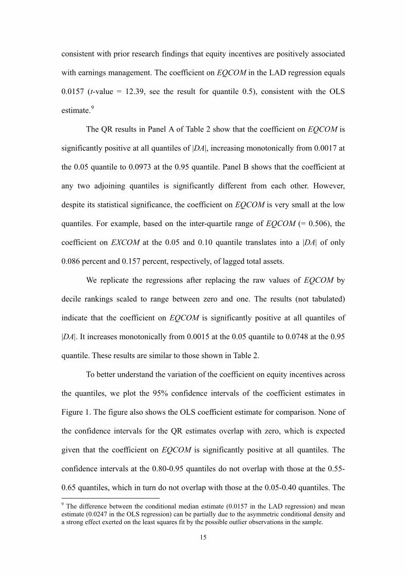
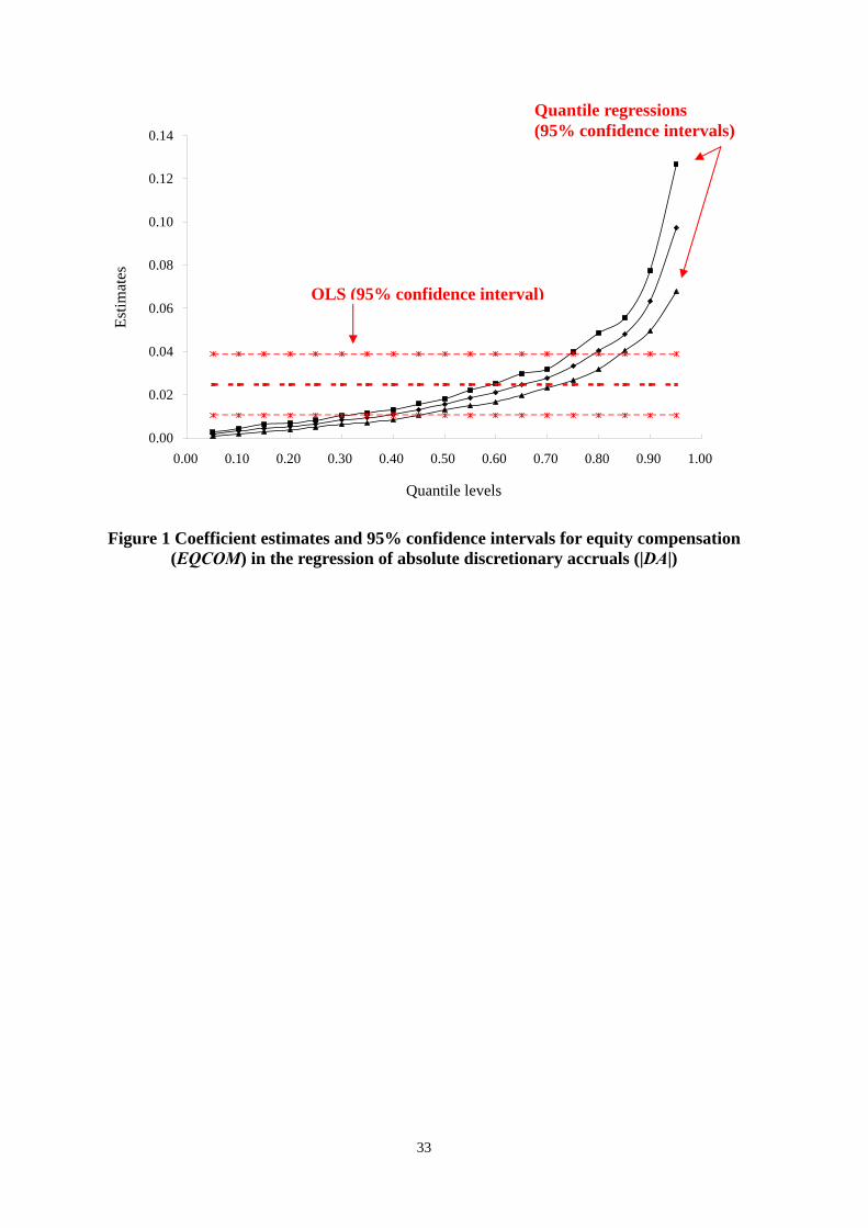
To better understand the variation of the coefficient on equity incentives across
the quantiles, we plot the 95% confidence intervals of the coefficient estimates in
Figure 1. The figure also shows the OLS coefficient estimate for comparison. None of
the confidence intervals for the QR estimates overlap with zero, which is expected
given that the coefficient on EQCOM is significantly positive at all quantiles. The
confidence intervals at the 0.80-0.95 quantiles do not overlap with those at the 0.55-
0.65 quantiles, which in turn do not overlap with those at the 0.05-0.40 quantiles. The 9 The difference between the conditional median estimate (0.0157 in the LAD regression) and mean estimate (0.0247 in the OLS regression) can be partially due to the asymmetric conditional density and a strong effect exerted on the least squares fit by the possible outlier observations in the sample.
15
95% confidence interval for the OLS estimate overlaps with only the QR estimates’
confidence intervals at the 0.35-0.80 quantiles. These findings show that the OLS
estimate does not capture the relation between CEO equity incentives and earnings
management at the high and low quantiles of absolute discretionary accruals (i.e.,
when the quality of financial reporting is very low or very high).
Taken together, the results in Table 2 and Figure 1 suggest that, on average,
higher equity incentives are associated with more extreme earnings management. But
the association is weaker when the firm has characteristics suggesting higher financial
reporting quality. When the quality of financial reporting is very high, the association
between equity incentives and earnings management becomes economically trivial,
and the OLS method overestimates the association.
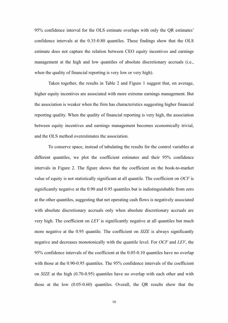
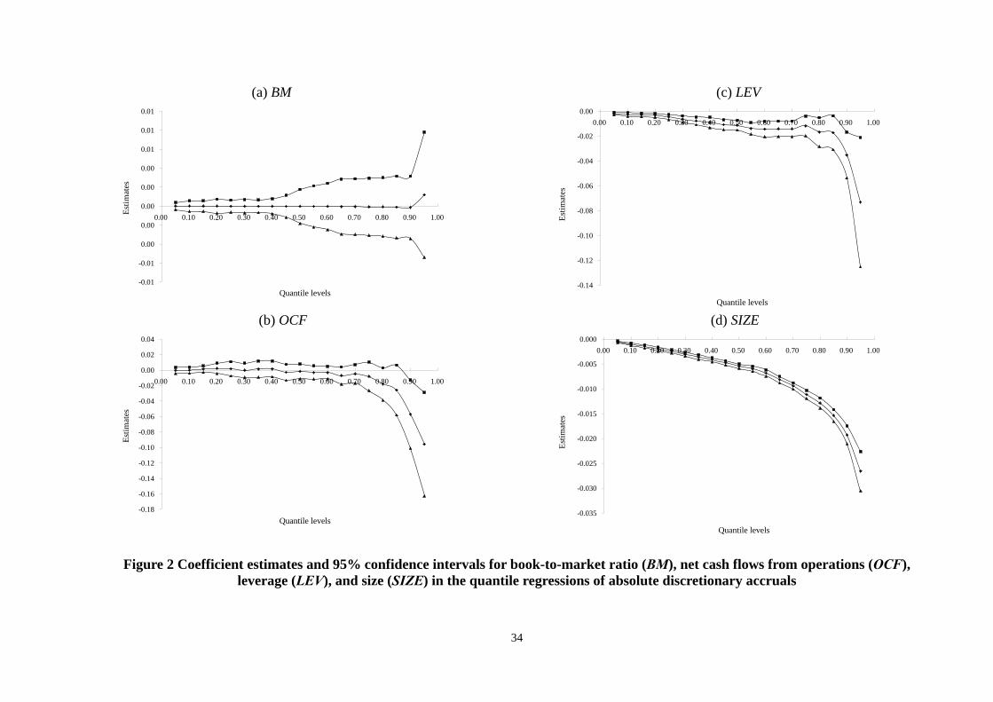
To conserve space, instead of tabulating the results for the control variables at
different quantiles, we plot the coefficient estimates and their 95% confidence
intervals in Figure 2. The figure shows that the coefficient on the book-to-market
value of equity is not statistically significant at all quantile. The coefficient on OCF is
significantly negative at the 0.90 and 0.95 quantiles but is indistinguishable from zero
at the other quantiles, suggesting that net operating cash flows is negatively associated
with absolute discretionary accruals only when absolute discretionary accruals are
very high. The coefficient on LEV is significantly negative at all quantiles but much
more negative at the 0.95 quantile. The coefficient on SIZE is always significantly
negative and decreases monotonically with the quantile level. For OCF and LEV, the
95% confidence intervals of the coefficient at the 0.05-0.10 quantiles have no overlap
with those at the 0.90-0.95 quantiles. The 95% confidence intervals of the coefficient
on SIZE at the high (0.70-0.95) quantiles have no overlap with each other and with
those at the low (0.05-0.60) quantiles. Overall, the QR results show that the
16
associations of net operating cash flows, leverage, and size with earnings management
are much stronger when the firm has lower financial reporting quality.10
5.3 Equity incentives and signed values of discretionary accruals
We replicate the above OLS and QR analyses using the signed values of
discretionary accruals (DA) as the dependent variable. The results for equity
incentives are presented in Table 3. Note that since the median (quantile 0.50) of DA
is close to zero, DA at the 0.55 quantile or above (0.45 quantile or below) in Table 3
are positive (negative).
Panel A of Table 3 shows that, in the OLS regression of DA, the coefficient on
EQCOM equals -0.0121 (t-value = -1.62). The LAD estimate of this coefficient equals
-0.0162 (t-value = -10.67, see the QR result at the 0.50 quantile in the same panel).
The QR results show that the coefficient on EQCOM increases monotonically with
the quantile level of DA, ranging from -0.0919 at the 0.05 quantile to 0.0266 at the
0.95 quantile, and the coefficient is significantly negative (positive) at the 0.05-0.65
(0.85-0.95) quantiles. Panel B shows that the coefficient at any two adjoining
quantiles is significantly different from each other.
When we replicate the regressions after replacing the raw values of EQCOM
by decile rankings scaled to range between zero and one, we find that the coefficient
on EQCOM increases monotonically from -0.0788 at the 0.05 quantile to 0.0208 at
the 0.95 quantile (results not tabulated). The coefficient is significantly negative
(positive) at the 0.05-0.70 (0.80-0.95) quantiles. These results are qualitatively similar
to those shown in Table 3.
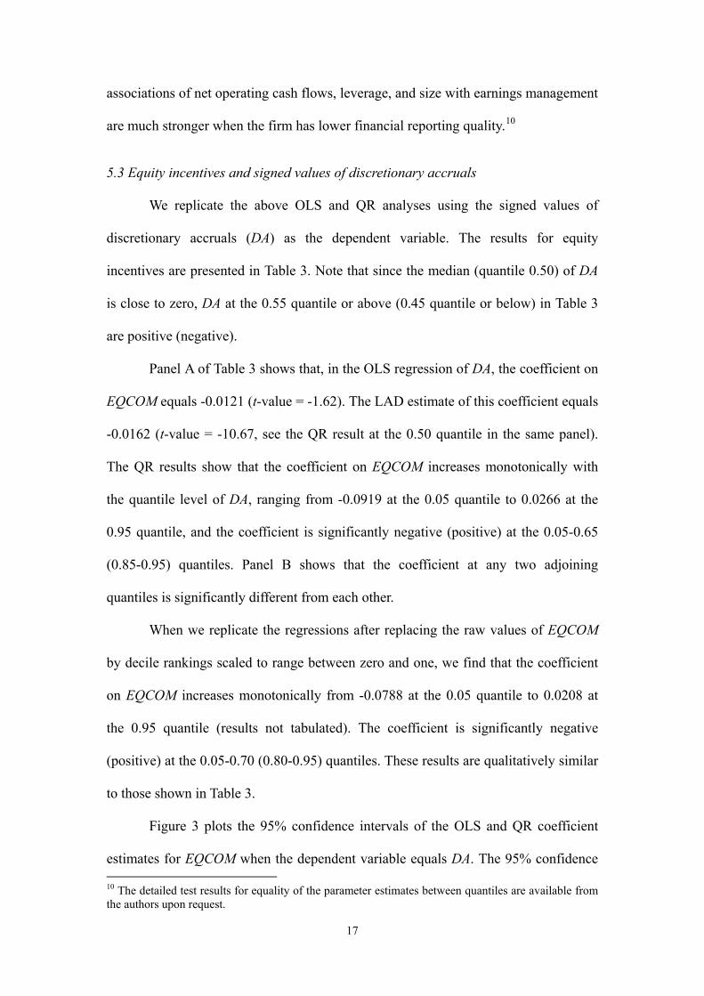
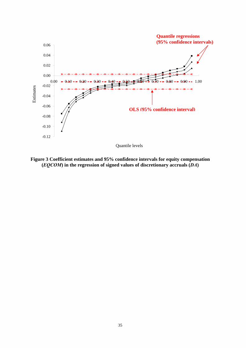
Figure 3 plots the 95% confidence intervals of the OLS and QR coefficient
estimates for EQCOM when the dependent variable equals DA. The 95% confidence 10 The detailed test results for equality of the parameter estimates between quantiles are available from the authors upon request.
17
intervals at the very high (0.90 and 0.95) and low (0.05 to 0.20) quantiles have no
overlap with the 95% confidence interval of the OLS estimate. Therefore, consistent
with the results from regression of |DA|, the findings in Table 3 and Figure 3 show
that the OLS estimate does not capture the relation between CEO equity incentives
and earnings management at the high and low quantiles of raw values of discretionary
accruals. Overall, the QR results show a positive association between equity
incentives and income-increasing earnings management only when the firm has
characteristics suggesting poor financial reporting quality (DA at high quantiles).
When the quality of financial reporting is relatively good, equity incentives are
negatively associated with income-increasing earnings management.
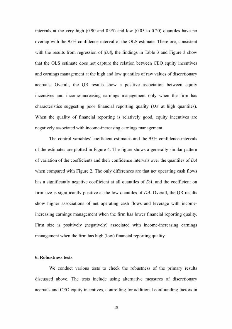
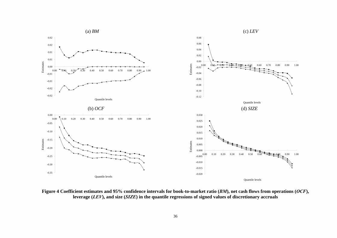
The control variables’ coefficient estimates and the 95% confidence intervals
of the estimates are plotted in Figure 4. The figure shows a generally similar pattern
of variation of the coefficients and their confidence intervals over the quantiles of DA
when compared with Figure 2. The only differences are that net operating cash flows
has a significantly negative coefficient at all quantiles of DA, and the coefficient on
firm size is significantly positive at the low quantiles of DA. Overall, the QR results
show higher associations of net operating cash flows and leverage with income-
increasing earnings management when the firm has lower financial reporting quality.
Firm size is positively (negatively) associated with income-increasing earnings
management when the firm has high (low) financial reporting quality.
6. Robustness tests
We conduct various tests to check the robustness of the primary results
discussed above. The tests include using alternative measures of discretionary
accruals and CEO equity incentives, controlling for additional confounding factors in
18
the regressions, using an instrumental variable approach to address the potential
endogeneity problem, and using a first-difference specification (i.e., changes model).
6.1 Using alternative measures of discretionary accruals and equity incentives
In the empirical analysis discussed above, we use discretionary accruals
adjusted for lagged performance, following the argument by Kothari, Leone, and
Wasley (2005) that performance-matched discretionary accrual measures enhance the
reliability of the inferences from earnings management research. Since some prior
studies on equity compensation and earnings management estimate discretionary
accruals using modified Jones model, we replicate all the regressions using this
alternative measure of discretionary accruals. The results (not shown) are similar to
those reported in the tables and figures. We also obtain similar regression results using
discretionary accruals adjusted for contemporaneous performance.
In the primary analysis we measure CEO equity incentives as total value of
restricted stock and stock options granted to the CEO divided by total compensation.
Some prior studies measure CEO equity incentives in a different way, such as the
pay-for-performance sensitivity and the value of stock options granted divided by
total compensation. Therefore, we replicate the regressions using these two alternative
measures of equity incentives.
Following the method in Core and Guay (2002), and Broussard, Buchenroth,
and Pilotte (2004), we define pay-for-performance sensitivity (PPS) as the partial
derivative of the Black-Scholes option value with respect to the stock price. 11
However, to mitigate the potential problem of heteroskedasticity, we use the natural
logarithm instead of the raw value.
11 Data on the Black-Scholes stock option values are no longer available on ExecuComp after 2006. To ensure use of consistent estimation method for option values across years, our analysis using PPS is limited to the 1995-2006 period.
19
Table 4, Panel A, shows the results for the regression of |DA| on PPS. The
OLS coefficient estimate for PPS is positive but not significantly different from zero.
The QR results show that the coefficient on PPS is positive but not statistically
significant at most of the below-median quantiles of |DA (except the 0.10 and 0.15
quantiles). However, the coefficient is significantly positive at all of the above-median
quantiles and increases with the quantile level. Untabulated results show that the
coefficient at each of the 0.65-0.95 quantiles is significantly different from the
coefficient at each of the 0.05-0.60 quantiles.
Table 4, Panel B, shows the results for the regression of DA on PPS. The OLS
coefficient estimate for PPS is negative but not significantly different from zero. The
QR results show that the coefficient on PPS is significantly negative at or below the
0.40 quantile and is significantly positive at the 0.95 quantile. Untabulated results
show that the coefficient at the 0.95 quantiles is significantly different from the
coefficient at the other quantiles.
Overall, the results when measuring the CEO equity incentives by
pay-for-performance sensitivity are qualitatively similar to those reported in Tables 2
and 3 for EQCOM. We also obtain similar results (not shown) when measuring the
CEO equity incentives by the ratio of stock option grants to total compensation
(Hanlon, et al. 2003).
6.2 Controlling for additional confounding factors
In the robustness tests we further control for several factors that could be
associated with discretionary accruals. Those factors include firm age, auditor type,
and audit opinion. Prior studies find that firms that are older or audited by a Big-N
auditor tend to have lower accruals, whereas firms that receive a qualified audit
opinion tend to have higher accruals. We measure firm age as the length of time (in
20
years) since the first year the firm’s financial data are available on Compustat.12
Auditor type is an indicator variable which equals one if the firm is audited by a
Big-N auditor an zero otherwise. Audit opinion is an indicator variable which equals
one if the firm receives a qualified audit opinion and zero otherwise. We also include
a set of indicator variables to control for the year effects. The results are similar to
those reported in Tables 2 and 3 after we include the above control variables in the
regressions.
6.3 Other robustness tests
Endogeneity could be a concern in empirical tests when the dependent and
independent variables are contemporaneous. To address this problem, we follow prior
studies to use the lagged value of equity compensation as an instrumental variable for
EQCOM and estimate the same QR model. The regression results (not tabulated) are
similar to those reported in the tables.
In the primary analyses we regress the level of discretionary accruals on the
level of equity incentives (equity-based compensation divided by total compensation).
This type of “levels model” could be subject to the correlated omitted variables
problem and may not be as powerful as the “changes model.” To address this concern,
we take the first difference of the variables in Equation (7) and estimate QR for the
new model. The regression results (not tabulated) are still similar to those reported in
the tables.
In summary, we conduct various robustness tests and find the QR results to be
largely consistent with those based on the models and measures of variables in the
primary analyses. The quantile-varying relationships between equity incentives and
12 We do not use the firm’s real age as it is not practical to collect such data manually for a large sample.
21
earnings management appear to be robust.
7. Summary and conclusions
The widespread use of equity-based compensation in executive compensation
packages has raised concerns that excessive equity compensation motivates earnings
management. A number of studies examine this issue but the evidence is not
conclusive. Our study contributes to this line of research by using a less restrictive
methodology and providing evidence that helps to reconcile the inconsistent results
among the prior studies. Specifically, we investigate the association between equity
compensation and earnings management using the quantile regression, which allows
the parameter estimates to vary over the distribution of the dependent variable. Unlike
the OLS and LAD regressions which rely on the central tendency distribution of the
dependent variable, the quantile regression also examines the dependent variable at
the tails of the distribution, thus facilitating an investigation of the relationship
between equity compensation and earnings management across the entire distribution
of the firms’ financial reporting quality.
We use discretionary accruals as a proxy for earnings management, where
higher (positive) accruals imply more income-increasing earnings management and
larger absolute discretionary accruals imply more extreme earnings management. We
measure equity compensation as the total value of restricted stock and stock options
granted to the CEO divided by the CEO’s total compensation, but we also use other
measures in the robustness tests. Our sample consists of 18,203 non-financial
firm-year observations in the U.S. (S&P 500 and medium and small cap) during the
period from 1995 to 2008.
The quantile regression results show that the association between equity
22
compensation and discretionary accruals varies substantially across the distribution of
the firms’ financial reporting quality (accruals), and some of the quantile regression
results are very different from the OLS regression results. We find that equity
compensation is positively associated with absolute discretionary accruals, but the
association is much stronger at the high quantiles of absolute discretionary accruals
and is economically trivial at the low quantiles. We also find that equity compensation
is positively associated with signed values of discretionary accruals only at the very
high quantiles of discretionary accruals, but it is negatively associated with signed
values of discretionary accruals at the low quantiles. The regression results are robust
to alternative measures of discretionary accruals and equity incentives and alternative
model specifications.
Overall, the evidence in our study suggests that equity compensation
motivates income-increasing earnings management only when the firm has
characteristics associated with lower financial reporting quality. We find no evidence
that equity compensation motivates earnings management when the firm’s financial
reporting quality is high. Our quantile regression results also demonstrate that the
OLS and LAD optimization techniques only capture the behaviors of firms with
financial reporting quality at the medium quantiles. Outside this range, the OLS and
LAD methods are more likely to overestimate (underestimate) the association
between equity compensation and earnings management as the firm’s financial
reporting quality moves towards the high (low) end.
23
References Abadie, A., J. Angrist, and G. Imbens. 2002. Instrumental variables estimates of the
effect of subsidized training on the quantiles of trainee earnings. Econometrica 70, 91-117.
Angrist, J., V. Chernozhukov, and I. Fernández-Val. 2006. Quantile regression under
misspecification, with an application to the U.S. wage structure. Econometrica 74, 539-563.
Armstrong, C. S., A. D. Jagolinzer, and D. F. Larcker. 2010. Chief executive officer
equity incentives and accounting irregularities. Journal of Accounting Research 48, 225-271.
Baber, W., S. Kang, and L. Liang. 2007. Shareholder rights, corporate governance,
and accounting restatement. Working paper, Georgetown University. Beasley, M. 1996. An empirical analysis of the relation between the board of director
composition and financial statement fraud. The Accounting Review 71, 443-465. Becker, C., M. DeFond, J. Jiambalvo, and K. Subramanyam. 1998. The effect of audit
quality on earnings management. Contemporary Accounting Research 15, 1-24. Bergstresser, D., and T. Philippon. 2006. CEO incentives and earnings management.
Journal of Financial Economics 80, 511-529. Broussard, J. P., S. A. Buchenroth, and E. A. Pilotte, 2004. CEO incentives, cash flow,
and investment. Financial Management 33, 51-70. Buchinsky, M. 1994. Changes in U.S. wage structure 1963-1987: An application of
quantile regression. Econometrica 62, 405-458. Buchinsky, M. 1998. Recent advances in quantile regression models. Journal of
Human Resources 27, 88-126. Burns, N., and S. Kedia. 2006. The impact of performance-based compensation on
misreporting. Journal of Financial Economics 79, 35-67. Cheng, Q., and T. D. Warfield. 2005. Equity incentives and earnings management.
The Accounting Review 80, 441-476. Chernozhukov, V., and C. Hansena. 2006. Instrumental quantile regression inference
for structural and treatment effect models. Journal of Econometrics 132, 491-525.
Core, J.E., and W. Guay. 2002. Estimating the value of employee stock option
portfolios and their sensitivities to price and volatility. Journal of Accounting Research 40, 613-630.
Core, J., R. Holthausen, and D. Larcker. 1999. Corporate governance, chief executive
24
officer compensation, and firm performance. Journal of Financial Economics 51, 371-406.
Dechow, P., R. Sloan, and A. Sweeney. 1995. Detecting earnings management. The
Accounting Review 70, 193-226. Dechow, P., R. Sloan, and A. Sweeney. 1996. Causes and consequences of earnings
manipulation: An analysis of firms subject to enforcement actions by the SEC. Contemporary Accounting Research 13, 1-36.
DeFond, M. L., and J. Jiambalvo. 1994. Debt covenant violation and manipulation of
accruals. Journal of Accounting and Economics 17, 145-177. Efendi, J., A. Srivastava, and E. P. Swanson. 2007. Why do corporate managers
misstate financial statements? The role of option compensation and other factors. Journal of Financial Economics 85, 667-708.
Erickson, M., M. Hanlon, and E. L. Maydew. 2006. Is there a link between executive
equity incentives and accounting fraud? Journal of Accounting Research 44, 113-143.
Francis, J. R., and J. Krishnan. 1999. Accounting accruals and auditor reporting
conservatism. Contemporary Accounting Research 16, 135-165. Gosling, A., S. Machin, and C. Meghir. 2000. The changing distribution of male
wages in the UK. Review of Economic Studies 67, 635-666. Graham, J. R., C. R. Harvey, and S. Rajgopal. 2005. The economic implications of
corporate financial reporting. Journal of Accounting and Economics 40, 3-73. Harris, J., and P. Bromiley. 2007. Incentives to cheat: The influence of executive
compensation and firm performance on financial misrepresentation. Organizational Science 18, 350-367.
Heckman, J. 1979. Sample selection bias as a specification error. Econometrica 47,
153-161. Holthausen, R. W., D. F. Larcker, and R. G. Sloan. 1995. Annual bonus schemes and
the manipulation of earnings. Journal of Accounting and Economics 19, 29-74. Jenkins, N. T. 2002. Auditor independence, audit committee effectiveness and
earnings management. Working paper, Washington University. Johnson, S. A., H. E. Ryan, and Y. S. Tian. 2009. Managerial incentives and corporate
fraud: The sources of incentives matters. Review of Finance 13, 115-145. Jones, J. J. 1991. Earnings management during import relief investigations. Journal of
Accounting Research 29, 193-228. Klein, A. 2002. Audit committee, board of director characteristics, and earnings
25
management. Journal of Accounting and Economics 33, 375-400. Koenker, R. 2000. Galton, edgeworth, frisch, and prospects for quantile regression in
econometrics. Journal of Econometrics 95, 347-374. Koenker, R., and G. Bassett. 1978. Regression quantiles. Econometrica 46, 33-50. Koenker, R., and K. F. Hallock. 2001. Quantile regression. Journal of Economic
Perspectives 15, 143-156. Kothari, S. P., A. J. Leone, and C. E. Wasley. 2005. Performance matched
discretionary accrual measures. Journal of Accounting and Economics 39, 163-197.
Larcker, D. F., and S. A. Richardson. 2004. Fees paid to audit firms, accrual choices,
and corporate governance. Journal of Accounting Research 42, 625-658. Larcker, D. F., S. A. Richardson, and I. Tuna. 2007. Corporate governance, accounting
outcomes, and organizational performance. The Accounting Review 82, 963-1008.
Levin, J. 2001. For whom the reductions count: A quantile regression analysis of class
size on scholastic achievement. Empirical Economics 26, 221-246. Menon, K., and D. D. Williams. 2004. Former audit partners and abnormal accruals.
The Accounting Review 79, 1095-1118. Mueller, R. 2000. Public- and private-sector wage differentials in Canada revisited.
Industrial Relations 39, 375-400. Myers, J. N., L. A. Myers, and T. C. Omer. 2003. Exploring the term of the
auditor-client relationship and the quality of earnings: A case for mandatory auditor rotation? The Accounting Review 78, 779-799.
O’Connor, J. P., R. L. Priem, J. E. Coombs, and K. M. Gilley. 2006. Do CEO stock
options prevent or promote fraudulent financial reporting? Academy of Management Journal 49, 483-500.
Richardson, S. A., A. I. Tuna, and M. Wu. 2003. Capital market pressures and
earnings management: The case of earnings restatements. Working paper, University of Pennsylvania.
Xie, B., W. N. Davidson, and P. J. Dadalt. 2002. Earnings management and corporate
governance: The roles of the board and the Audit Committee. Working paper, Southern Illinois University.
26
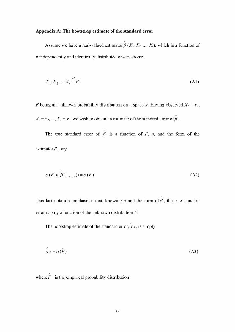
Appendix A: The bootstrap estimate of the standard error
Assume we have a real-valued estimator (X∧
β 1, X2, ..., Xn), which is a function of
n independently and identically distributed observations:
,~,...,, 21 FXXXiid
n (A1)
F being an unknown probability distribution on a space κ. Having observed X1 = x1,
X2 = x2, ..., Xn = xn, we wish to obtain an estimate of the standard error of . ∧
β
The true standard error of is a function of F, n, and the form of the
estimator , say
∧
β
∧
β
).())(.,.,...,.,,( FnF σβσ =∧
(A2)
This last notation emphasizes that, knowing n and the form of , the true standard
error is only a function of the unknown distribution F.
∧
β
The bootstrap estimate of the standard error, , is simply B
∧
σ
),(∧∧
= FB σσ (A3)
where∧
F is the empirical probability distribution
27
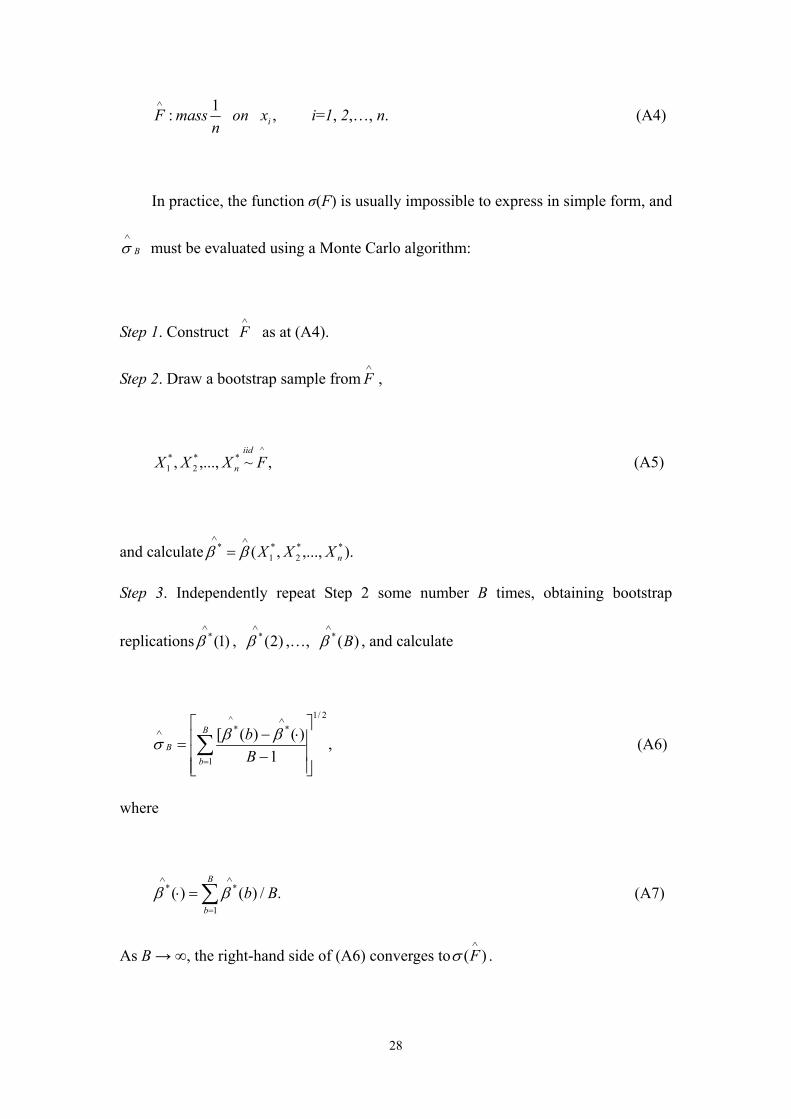
,1: ixonn
massF∧
i=1, 2,…, n. (A4)
In practice, the function σ(F) is usually impossible to express in simple form, and
must be evaluated using a Monte Carlo algorithm: B
∧
σ
Step 1. Construct ∧
F as at (A4).
Step 2. Draw a bootstrap sample from∧
F ,
,~,...,,^
**2
*1 FXXX
iid
n (A5)
and calculate ).,...,,( **2
*1
*nXXX
∧∧
= ββ
Step 3. Independently repeat Step 2 some number B times, obtaining bootstrap
replications , ,…, , and calculate )1(*∧
β )2(*∧
β )(* B∧
β
,1
)()([2/1
1
*^
*
⎥⎥⎥
⎦
⎤
⎢⎢⎢
⎣
⎡
−⋅−
= ∑=
∧∧ B
bB
Bb ββσ (A6)
where
./)()(1
** BbB
b∑=
∧∧
=⋅ ββ (A7)
As B → ∞, the right-hand side of (A6) converges to . )(
∧
Fσ
28
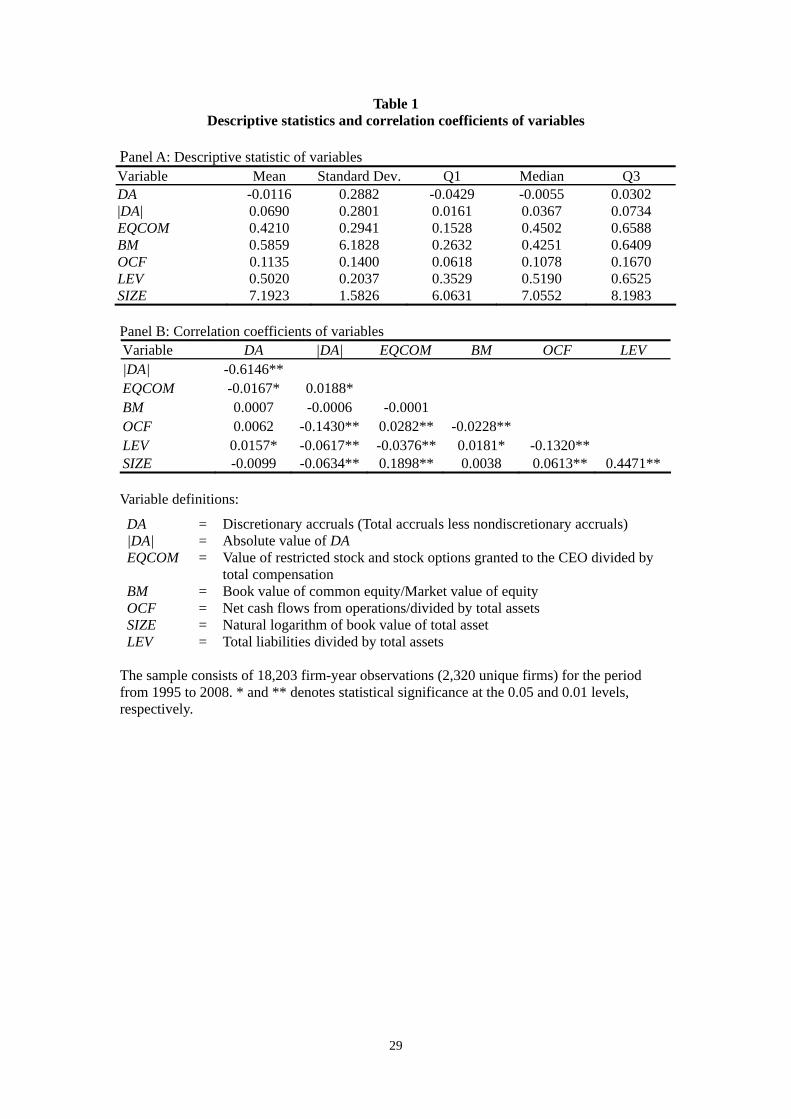
Table 1 Descriptive statistics and correlation coefficients of variables
Panel A: Descriptive statistic of variables Variable Mean Standard Dev. Q1 Median Q3 DA -0.0116 0.2882 -0.0429 -0.0055 0.0302 |DA| 0.0690 0.2801 0.0161 0.0367 0.0734 EQCOM 0.4210 0.2941 0.1528 0.4502 0.6588 BM 0.5859 6.1828 0.2632 0.4251 0.6409 OCF 0.1135 0.1400 0.0618 0.1078 0.1670 LEV 0.5020 0.2037 0.3529 0.5190 0.6525 SIZE 7.1923 1.5826 6.0631 7.0552 8.1983
Panel B: Correlation coefficients of variables Variable DA |DA| EQCOM BM OCF LEV |DA| -0.6146**
EQCOM -0.0167* 0.0188*
BM 0.0007 -0.0006 -0.0001
OCF 0.0062 -0.1430** 0.0282** -0.0228**
LEV 0.0157* -0.0617** -0.0376** 0.0181* -0.1320**
SIZE -0.0099 -0.0634** 0.1898** 0.0038 0.0613** 0.4471** Variable definitions:
DA = Discretionary accruals (Total accruals less nondiscretionary accruals) |DA| = Absolute value of DA EQCOM = Value of restricted stock and stock options granted to the CEO divided by
total compensation BM = Book value of common equity/Market value of equity OCF = Net cash flows from operations/divided by total assets SIZE = Natural logarithm of book value of total asset LEV = Total liabilities divided by total assets
The sample consists of 18,203 firm-year observations (2,320 unique firms) for the period from 1995 to 2008. * and ** denotes statistical significance at the 0.05 and 0.01 levels, respectively.
29
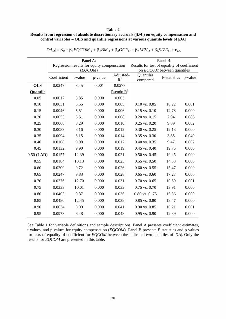
Table 2 Results from regression of absolute discretionary accruals (|DA|) on equity compensation and
control variables – OLS and quantile regressions at various quantile levels of |DA|
|DAi,t| = β0 + β1EQCOMi,t + β2BMi,t + β3OCFi,t + β4LEVi,t + β5SIZEi,t + εi,t,
Panel A:
Regression results for equity compensation (EQCOM)
Panel B: Results for test of equality of coefficient
on EQCOM between quantiles
Coefficient t-value p-value Adjusted-R2
Quantiles compared F-statistics p-value
OLS 0.0247 3.45 0.001 0.0278 Quantile Pseudo R2
0.05 0.0017 3.85 0.000 0.003 0.10 0.0031 5.55 0.000 0.005 0.10 vs. 0.05 10.22 0.001
0.15 0.0046 5.51 0.000 0.006 0.15 vs. 0.10 12.73 0.000
0.20 0.0053 6.51 0.000 0.008 0.20 vs. 0.15 2.94 0.086
0.25 0.0066 8.29 0.000 0.010 0.25 vs. 0.20 9.89 0.002
0.30 0.0083 8.16 0.000 0.012 0.30 vs. 0.25 12.13 0.000
0.35 0.0094 8.15 0.000 0.014 0.35 vs. 0.30 3.85 0.049
0.40 0.0108 9.08 0.000 0.017 0.40 vs. 0.35 9.47 0.002
0.45 0.0132 9.90 0.000 0.019 0.45 vs. 0.40 19.75 0.000
0.50 (LAD) 0.0157 12.39 0.000 0.021 0.50 vs. 0.45 19.45 0.000
0.55 0.0184 10.13 0.000 0.023 0.55 vs. 0.50 14.53 0.000
0.60 0.0209 9.72 0.000 0.026 0.60 vs. 0.55 15.47 0.000
0.65 0.0247 9.83 0.000 0.028 0.65 vs. 0.60 17.27 0.000
0.70 0.0276 12.70 0.000 0.031 0.70 vs. 0.65 10.59 0.001
0.75 0.0333 10.01 0.000 0.033 0.75 vs. 0.70 13.91 0.000
0.80 0.0403 9.37 0.000 0.036 0.80 vs. 0. 75 15.36 0.000
0.85 0.0480 12.45 0.000 0.038 0.85 vs. 0.80 13.47 0.000
0.90 0.0634 8.99 0.000 0.041 0.90 vs. 0.85 10.21 0.001
0.95 0.0973 6.48 0.000 0.048 0.95 vs. 0.90 12.39 0.000
See Table 1 for variable definitions and sample descriptions. Panel A presents coefficient estimates, t-values, and p-values for equity compensation (EQCOM). Panel B presents F-statistics and p-values for tests of equality of coefficient for EQCOM between the indicated two quantiles of |DA|. Only the results for EQCOM are presented in this table.
30
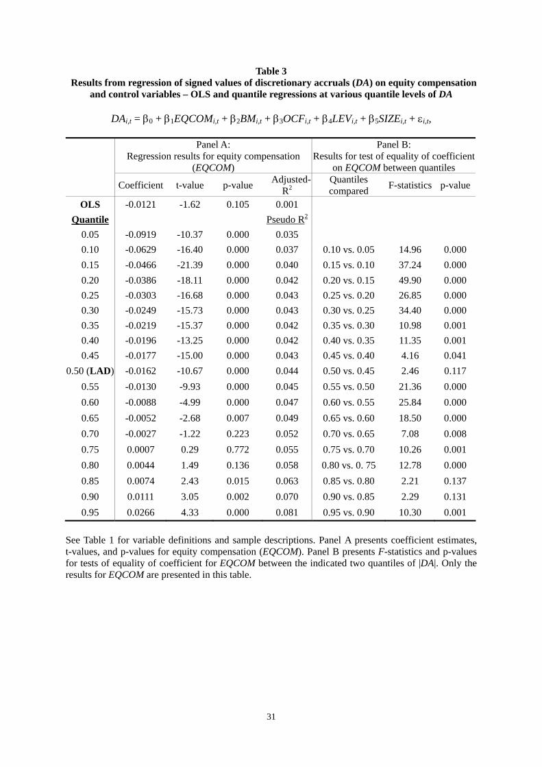
Table 3 Results from regression of signed values of discretionary accruals (DA) on equity compensation
and control variables – OLS and quantile regressions at various quantile levels of DA
DAi,t = β0 + β1EQCOMi,t + β2BMi,t + β3OCFi,t + β4LEVi,t + β5SIZEi,t + εi,t,
Panel A:
Regression results for equity compensation (EQCOM)
Panel B: Results for test of equality of coefficient
on EQCOM between quantiles
Coefficient t-value p-value Adjusted-R2
Quantiles compared F-statistics p-value
OLS -0.0121 -1.62 0.105 0.001 Quantile Pseudo R2
0.05 -0.0919 -10.37 0.000 0.035 0.10 -0.0629 -16.40 0.000 0.037 0.10 vs. 0.05 14.96 0.000
0.15 -0.0466 -21.39 0.000 0.040 0.15 vs. 0.10 37.24 0.000
0.20 -0.0386 -18.11 0.000 0.042 0.20 vs. 0.15 49.90 0.000
0.25 -0.0303 -16.68 0.000 0.043 0.25 vs. 0.20 26.85 0.000
0.30 -0.0249 -15.73 0.000 0.043 0.30 vs. 0.25 34.40 0.000
0.35 -0.0219 -15.37 0.000 0.042 0.35 vs. 0.30 10.98 0.001
0.40 -0.0196 -13.25 0.000 0.042 0.40 vs. 0.35 11.35 0.001
0.45 -0.0177 -15.00 0.000 0.043 0.45 vs. 0.40 4.16 0.041
0.50 (LAD) -0.0162 -10.67 0.000 0.044 0.50 vs. 0.45 2.46 0.117
0.55 -0.0130 -9.93 0.000 0.045 0.55 vs. 0.50 21.36 0.000
0.60 -0.0088 -4.99 0.000 0.047 0.60 vs. 0.55 25.84 0.000
0.65 -0.0052 -2.68 0.007 0.049 0.65 vs. 0.60 18.50 0.000
0.70 -0.0027 -1.22 0.223 0.052 0.70 vs. 0.65 7.08 0.008
0.75 0.0007 0.29 0.772 0.055 0.75 vs. 0.70 10.26 0.001
0.80 0.0044 1.49 0.136 0.058 0.80 vs. 0. 75 12.78 0.000
0.85 0.0074 2.43 0.015 0.063 0.85 vs. 0.80 2.21 0.137
0.90 0.0111 3.05 0.002 0.070 0.90 vs. 0.85 2.29 0.131
0.95 0.0266 4.33 0.000 0.081 0.95 vs. 0.90 10.30 0.001
See Table 1 for variable definitions and sample descriptions. Panel A presents coefficient estimates, t-values, and p-values for equity compensation (EQCOM). Panel B presents F-statistics and p-values for tests of equality of coefficient for EQCOM between the indicated two quantiles of |DA|. Only the results for EQCOM are presented in this table.
31
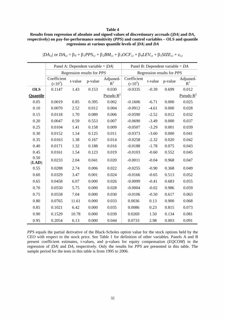
Table 4 Results from regression of absolute and signed values of discretionary accruals (|DA| and DA,
respectively) on pay-for-performance sensitivity (PPS) and control variables – OLS and quantile regressions at various quantile levels of |DA| and DA
|DAi,t| or DAi,t = β0 + β1PPSi,t + β2BMi,t + β3OCFi,t + β4LEVi,t + β5SIZEi,t + εi,t
Panel A: Dependent variable = |DA| Panel B: Dependent variable = DA Regression results for PPS Regression results for PPS
Coefficient (×103) t-value p-value Adjusted-
R2Coefficient
(×103) t-value p-value Adjusted-R2
OLS 0.1147 1.43 0.153 0.030 -0.0335 -0.39 0.699 0.012
Quantile Pseudo R2 Pseudo R2
0.05 0.0019 0.85 0.395 0.002 -0.1606 -6.71 0.000 0.025
0.10 0.0070 2.52 0.012 0.004 -0.0912 -4.61 0.000 0.028
0.15 0.0118 1.70 0.089 0.006 -0.0590 -2.52 0.012 0.032
0.20 0.0047 0.59 0.553 0.007 -0.0690 -3.49 0.000 0.037
0.25 0.0104 1.41 0.158 0.009 -0.0507 -3.29 0.001 0.039
0.30 0.0152 1.54 0.125 0.011 -0.0373 -3.60 0.000 0.041
0.35 0.0163 1.38 0.167 0.014 -0.0258 -2.32 0.020 0.042
0.40 0.0171 1.32 0.188 0.016 -0.0188 -1.78 0.075 0.043
0.45 0.0161 1.54 0.123 0.019 -0.0103 -0.60 0.552 0.045
0.50 (LAD) 0.0233 2.04 0.041 0.020 -0.0011 -0.04 0.968 0.047
0.55 0.0288 2.74 0.006 0.022 -0.0255 -0.90 0.368 0.049
0.60 0.0329 3.47 0.001 0.024 -0.0166 -0.65 0.513 0.052
0.65 0.0458 6.07 0.000 0.026 -0.0099 -0.41 0.683 0.055
0.70 0.0550 5.75 0.000 0.028 -0.0004 -0.02 0.986 0.059
0.75 0.0558 7.04 0.000 0.030 -0.0106 -0.50 0.617 0.063
0.80 0.0765 11.61 0.000 0.033 0.0036 0.13 0.900 0.068
0.85 0.1021 6.42 0.000 0.035 0.0086 0.23 0.815 0.073
0.90 0.1529 10.78 0.000 0.039 0.0269 1.50 0.134 0.081
0.95 0.2054 6.13 0.000 0.044 0.0733 2.98 0.003 0.091
PPS equals the partial derivative of the Black-Scholes option value for the stock options held by the CEO with respect to the stock price. See Table 1 for definition of other variables. Panels A and B present coefficient estimates, t-values, and p-values for equity compensation (EQCOM) in the regression of |DA| and DA, respectively. Only the results for PPS are presented in this table. The sample period for the tests in this table is from 1995 to 2006.
32
0.00
0.02
0.04
0.06
0.08
0.10
0.12
0.14
0.00 0.10 0.20 0.30 0.40 0.50 0.60 0.70 0.80 0.90 1.00
Quantile levels
Estim
ates
Quantile regressions (95% confidence intervals)
OLS (95% confidence interval)
Figure 1 Coefficient estimates and 95% confidence intervals for equity compensation
(EQCOM) in the regression of absolute discretionary accruals (|DA|)
33
(a) BM (c) LEV
-0.01
-0.01
0.00
0.00
0.00
0.00
0.00
0.01
0.01
0.01
0.00 0.10 0.20 0.30 0.40 0.50 0.60 0.70 0.80 0.90 1.00
Quantile levels
Estim
ates
-0.14
-0.12
-0.10
-0.08
-0.06
-0.04
-0.02
0.000.00 0.10 0.20 0.30 0.40 0.50 0.60 0.70 0.80 0.90 1.00
Quantile levels
Estim
ates
(b) OCF (d) SIZE
-0.18
-0.16
-0.14
-0.12
-0.10
-0.08
-0.06
-0.04
-0.02
0.00
0.02
0.04
0.00 0.10 0.20 0.30 0.40 0.50 0.60 0.70 0.80 0.90 1.00
Quantile levels
Estim
ates
-0.035
-0.030
-0.025
-0.020
-0.015
-0.010
-0.005
0.0000.00 0.10 0.20 0.30 0.40 0.50 0.60 0.70 0.80 0.90 1.00
Quantile levels
Estim
ates
Figure 2 Coefficient estimates and 95% confidence intervals for book-to-market ratio (BM), net cash flows from operations (OCF), leverage (LEV), and size (SIZE) in the quantile regressions of absolute discretionary accruals
34
-0.12
-0.10
-0.08
-0.06
-0.04
-0.02
0.00
0.02
0.04
0.06
0.00 0.10 0.20 0.30 0.40 0.50 0.60 0.70 0.80 0.90 1.00
Quantile levels
Estim
ates
Quantile regressions (95% confidence intervals)
OLS (95% confidence interval)
Figure 3 Coefficient estimates and 95% confidence intervals for equity compensation
(EQCOM) in the regression of signed values of discretionary accruals (DA)
35
(a) BM (c) LEV
-0.02
-0.02
-0.01
-0.01
0.00
0.01
0.01
0.02
0.02
0.00 0.10 0.20 0.30 0.40 0.50 0.60 0.70 0.80 0.90 1.00
Quantile levels
Estim
ates
-0.12
-0.10
-0.08
-0.06
-0.04
-0.02
0.00
0.02
0.04
0.06
0.08
0.00 0.10 0.20 0.30 0.40 0.50 0.60 0.70 0.80 0.90 1.00
Quantile levels
Estim
ates
(b) OCF (d) SIZE
-0.35
-0.30
-0.25
-0.20
-0.15
-0.10
-0.05
0.000.00 0.10 0.20 0.30 0.40 0.50 0.60 0.70 0.80 0.90 1.00
Quantile levels
Estim
ates
-0.020
-0.015
-0.010
-0.005
0.000
0.005
0.010
0.015
0.020
0.025
0.030
0.00 0.10 0.20 0.30 0.40 0.50 0.60 0.70 0.80 0.90 1.00
Quantile levels
Estim
ates
Figure 4 Coefficient estimates and 95% confidence intervals for book-to-market ratio (BM), net cash flows from operations (OCF), leverage (LEV), and size (SIZE) in the quantile regressions of signed values of discretionary accruals
36