Exercise 3: Advanced Material Models (Plasticity and ... · Exercise 3: Advanced Material Models (Plasticity and ... (click on Worksheet and right-click EPPLX → Create User Defined

www.uni-ulm.de/uzwr 1 / 8

Computational Methods in Materials Science – Lab 3 F. Niemeyer, U. Simon

Exercise 3: Advanced Material

Models (Plasticity and Anisotropy)

Goals Today you will learn how to use advanced material models beyond linear isotropic elasticity.

We will first have a look at plasticity with strain hardening. Then we will switch to wood as an

example for anisotropic material behavior.

1. Cold Forming For this first task, we will use a cantilever beam geometry, very similar to the previous models

you built (cf. Figure 1). Use the provided data in Table 1 to create the beam using Design-

Modeler.

Figure 1: Cantilever beam with load F applied at the right end

Given:

Table 1: Geometry and material data

� 1000 mm Beam length ℎ 60 mm Beam height � 40 mm Beam thickness

�� 22 000 N Force for load step 1 �� −25 000 N Force for load step 2 � 0 N Force for load step 3 73 100 MPa Young’s modulus of aluminium � 0.33 Poisson’s ratio

� 7310 MPa Tangent modulus �� 414 MPa Yield strength



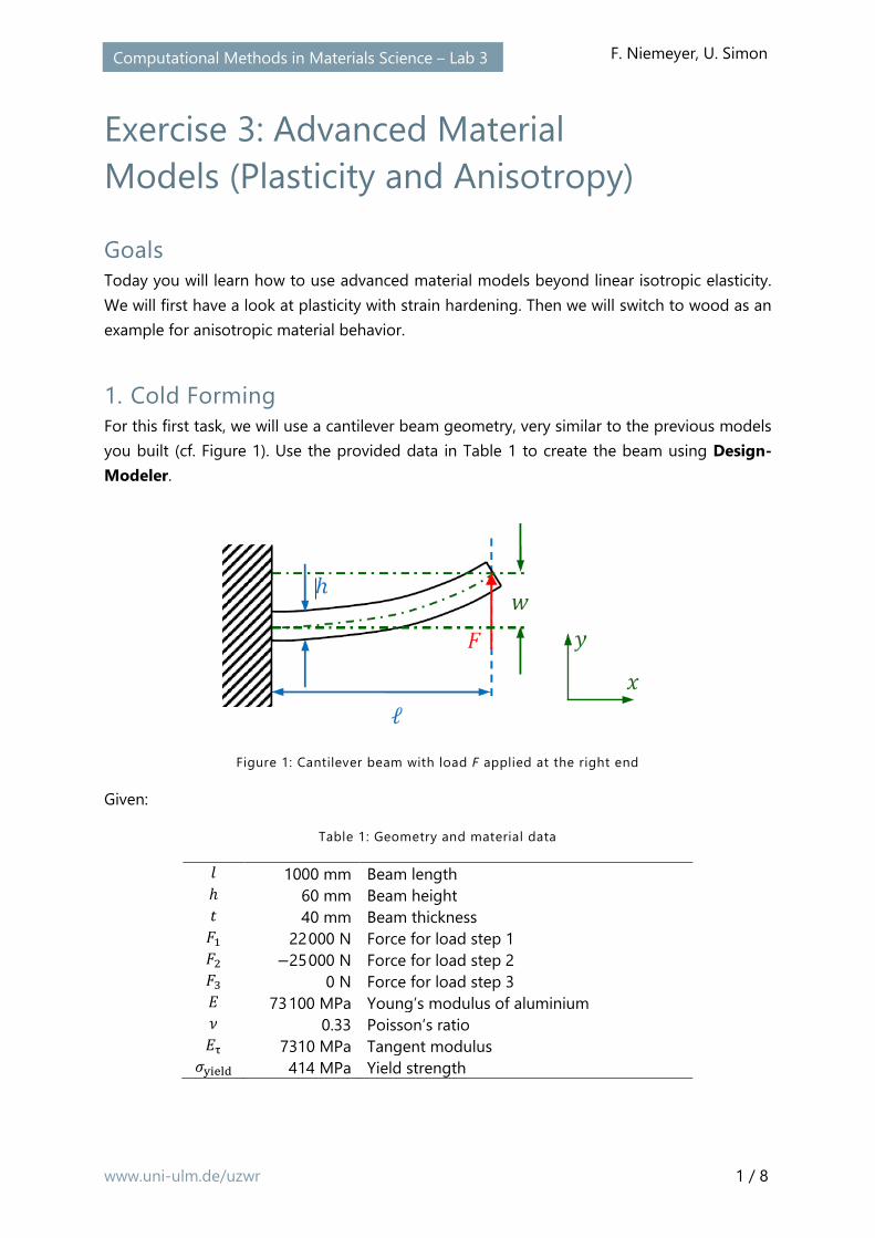
Add a new material to your Engineering Data. Use the material properties provided by Table

1 to define both the material’s Isotropic Elasticity as well as Bilinear Isotropic Hardening

(drag and drop from the Toolbox). Afterwards, selecting Bilinear Isotropic Hardening in the

properties windows should bring up a stress-strain curve resembling Figure 2.

Figure 2: Stress-strain curve for our elasto-plastic material

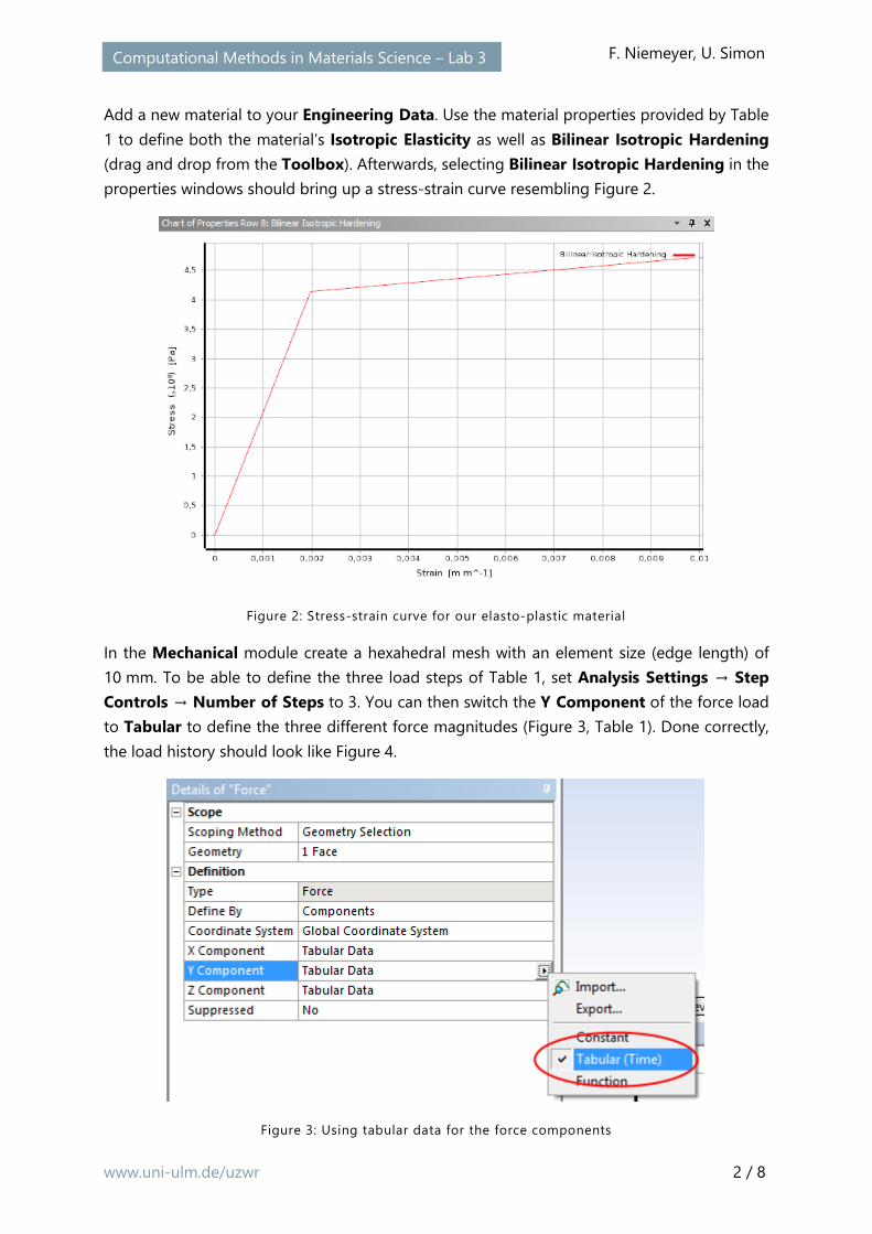
In the Mechanical module create a hexahedral mesh with an element size (edge length) of

10 mm. To be able to define the three load steps of Table 1, set Analysis Settings → Step

Controls → Number of Steps to 3. You can then switch the Y Component of the force load

to Tabular to define the three different force magnitudes (Figure 3, Table 1). Done correctly,

the load history should look like Figure 4.

Figure 3: Using tabular data for the force components



Figure 4: Load history with three distinct steps

Choose Force Convergence under Solution (A6) → Solution Information → Solution Out-

put. Also, enable support for large deformations by setting Analysis Settings → Solver Con-

trols → Large Deflection to On.

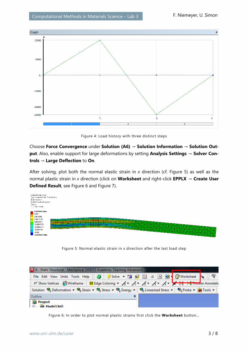
After solving, plot both the normal elastic strain in x direction (cf. Figure 5) as well as the

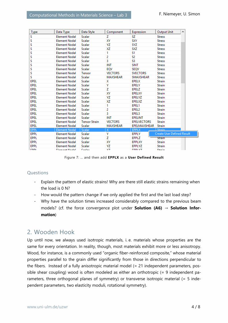
normal plastic strain in x direction (click on Worksheet and right-click EPPLX → Create User

Defined Result, see Figure 6 and Figure 7).

Figure 5: Normal elastic strain in x direction after the last load step

Figure 6: In order to plot normal plastic strains first click the Worksheet button…



Figure 7: … and then add EPPLX as a User Defined Result

Questions

- Explain the pattern of elastic strains! Why are there still elastic strains remaining when

the load is 0 N?

- How would the pattern change if we only applied the first and the last load step?

- Why have the solution times increased considerably compared to the previous beam

models? (cf. the force convergence plot under Solution (A6) → Solution Infor-

mation)

2. Wooden Hook Up until now, we always used isotropic materials, i. e. materials whose properties are the

same for every orientation. In reality, though, most materials exhibit more or less anisotropy.

Wood, for instance, is a commonly used “organic fiber-reinforced composite,” whose material

properties parallel to the grain differ significantly from those in directions perpendicular to

the fibers. Instead of a fully anisotropic material model (= 21 independent parameters, pos-

sible shear coupling) wood is often modeled as either an orthotropic (= 9 independent pa-

rameters, three orthogonal planes of symmetry) or transverse isotropic material (= 5 inde-

pendent parameters, two elasticity moduli, rotational symmetry).



We will use an orthotropic material model to describe the mechanical behavior of a solid

body made of a piece of wood. First, we need to agree on a material coordinate system. For

wood, it is common to consider the direction parallel to the grain the x (or longitudinal) di-

rection; the direction normal to the growth rings is the y (or radial direction); and finally, z is

the direction tangential to the growth rings (Figure 8).

Figure 8: Right-handed material coordinate system for wood

Create a new Static Structural analysis system (or an entirely new project). Then add a new

orthotropic material model (Engineering Data → Linear Elastic → Orthotropic Elasticity).

Extract the 9 required material parameters from the following PDF file about the material

properties of different wood types (pages 2 – 8)

→ http://www.woodweb.com/Resources/wood_eng_handbook/Ch04.pdf

You can choose any type of wood you’d like, e. g. pine. Just make sure that your material

properties use the coordinate system of Figure 8.

Next, start DesignModeler. We will use a slightly more sophisticated geometry this time.

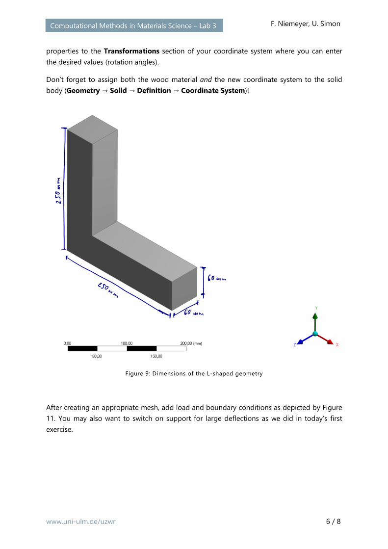
Create the geometry using two box primitives to produce an L-shaped form, corresponding

to Figure 9.

Ensure that the result is a single body, not two bodies/two separate parts! When you are done

with the geometry, start the Mechanical module.

By default, the coordinate system of each solid body – and hence its material – is the global

coordinate system. Because we want to investigate the influence of different material align-

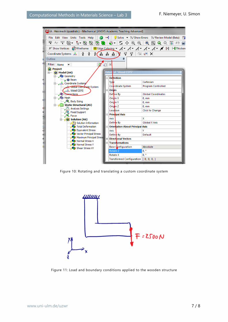
ment, we need to define a custom coordinate system: Right click on Coordinate Systems in

the Outline and insert a new Coordinate System (and give it a distinct name).

To rotate or translate the coordinate system, select it from the outline and click on the corre-

sponding buttons in the toolbar (Figure 10). This will add Rotate X/Y/Z or Translate X/Y/Z



properties to the Transformations section of your coordinate system where you can enter

the desired values (rotation angles).

Don’t forget to assign both the wood material and the new coordinate system to the solid

body (Geometry → Solid → Definition → Coordinate System)!

Figure 9: Dimensions of the L-shaped geometry

After creating an appropriate mesh, add load and boundary conditions as depicted by Figure

11. You may also want to switch on support for large deflections as we did in today’s first

exercise.



Figure 10: Rotating and translating a custom coordinate system

Figure 11: Load and boundary conditions applied to the wooden structure



Questions

- Why didn’t we have to define �� , �� and ��?

- Plot and compare principal strains and stresses (vector plots). What would you expect

to see, had we used an isotropic material instead?

- Where do you see compression, where tension?

- Try out different fiber alignments (e. g. 45°, 90°, 135°, –45° …). Which material orienta-

tion leads to the lowest amount of deformation? Why?

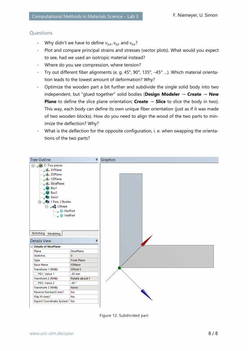
- Optimize the wooden part a bit further and subdivide the single solid body into two

independent, but “glued together” solid bodies (Design Modeler → Create → New

Plane to define the slice plane orientation; Create → Slice to slice the body in two).

This way, each body can define its own unique fiber orientation (just as if it was made

of two wooden blocks). How do you need to align the wood of the two parts to min-

imize the deflection? Why?

- What is the deflection for the opposite configuration, i. e. when swapping the orienta-

tions of the two parts?

Figure 12: Subdivided part

Documents

Exercise 3: Advanced Material Models (Plasticity and ... · Exercise 3: Advanced Material Models (Plasticity and ... (click on Worksheet and right-click EPPLX → Create User Defined