Exercise Manual for BIOL 471 Methods in Systematics

Exercise Manual for BIOL 471

Methods in Systematics Spring 2007

by Christopher R. Hardy, James C. Parks Herbarium, Dept. of Biology, Millersville University

Millersville, Pennsylvania USA

Methods in Systematics, page 2 of 62

BIOL 471 – Methods in Systematics

Exercise Manual Table of Contents

Exercise page Biotic Inventory & Related Activities Exercise 01: Traditional Dichotomous Keys and Biotic Inventory ................................................ 4 Exercise 02: Interactive Key Construction ..................................................................................... 8 Biogeographic Mapping, Analysis, and Modeling Exercise 01: DIVA-GIS Tutorial .................................................................................................. 14 Exercise 02: DIVA-GIS: Distribution and Diversity of Wild Potatoes........................................ 28 Exercise 03: Distribution and Diversity of Parks Herbarium Specimens..................................... 34 Exercise 04: Georeferencing and Generating Distribution Maps ................................................. 39 Exercise 05: DIVA-GIS: Biogeographic (Distribution) Modeling using Herbarium Specimens and Climate Data........................................................................................................................... 41 Phylogenetic Inference Exercise 01: Simple, Manual Cladogram Construction................................................................ 48 Exercise 02: Character State Optimization for Choosing Most Parsimonious Cladograms and Reconstructing Ancestral States. .................................................................................................. 51 Exercise 03: Morphological Datamatrix Construction and Basic Cladistic Analysis .................. 53 Exercise 04: DNA Sequences for Phylogenetic Inference ........................................................... 55 Species Delimitation, Diagnostics, and Conservation Forensics Exercise 01: Species Delimitation using Population Aggregation Analysis ................................ 58 Exercise 02: DNA in Species Delimitation, Diagnostics, and Conservation Forensics ............... 61


Biotic Inventory & Related Activities:

Interactive Key Construction


Exercise 01. Traditional Dichotomous Keys and Biotic Inventory One of the most important activities systematists do is conduct biotic inventories. We will conduct a biotic inventory of the genera of conifers on campus. Since we are not yet experts in identification, we will use a traditional dichotomous key to identify the genera of conifers that we have on campus (next page). Once we have this inventory, we will prepare an interactive key that will be posted online (at the Herbarium website) and will be used by future classes and other botanical enthusiasts of the MU Community. Procedure for today and as homework: 1. Collect conifers around campus. 2. Key them out to genus. 3. Construct a working checklist of the genera on MU campus. 4. Enter these alphabetically into the rows of datamatrix or spreadsheet. 5. Make a master list of the structural characteristics by which they differ. 6. Sort and name these characteristics (and their states) logically. 7. Enter these “characters” and “character states” logically as column headers in your datamatrix or spreadsheet. 8. Score these species for the appropriate character states. Use your specimens and literature to complete this.


A. Plants not evergreen B. Branchlets short and stubby, persistent, alternate.......................................Larix, Larch BB. Branchlets elongate, deciduous, opposite.....................Metasequoia, Dawn Redwood AA. Plants evergreen C. Leaves needle-shaped or otherwise elongate and well-diverging from the stem D. Leaves in fascicles of 2, 3, or 5.........................................................Pinus, Pine DD. Leaves borne singly or tufted on stubby side-branches (but not fascicled) E. Leaves tufted on stubby side-branches.......................... . Cedrus, Cedar EE. Leaves borne singly F. Leaf ending at stem so that stem is woody in texture & color. G. Leaves sharp-pointed and square in cross-section, with small woody peg-like leaf-stalk.................... Picea, Spruce GG. Leaves round-pointed and flattened, woody peg-like leaf-stalk absent or if present not very prominent H. Leaves usually <1.5 cm long, with distinct leaf- stalk; cones 1-2 cm long ...............Tsuga, Hemlock HH. Leaves >1.5 cm long, with no distinct leaf- stalk (although perhaps with a gradually narrowed leaf-base); cones >2.5 cm long I. Cones erect with scales deciduous at maturity; needle-base swollen and round, leaving a round leaf-scar...............Abies, Fir II. Cones pendulous, scales persistent, with very long 3-lobed bractsthat look like the rear-end of a mouse; needle-base not swollen, leaf-scar either not round or not very big...............Pseudotsuga, Douglas Fir FF. Leaf-base decurrent along (i.e., the base runs along) the stem for some distance, such that twig stem to which leaves are attached appears green. J. Leaves flattened and round pointed; cones with just a single seed which is partially enclosed in fleshy red aril; often bushes or shrubs.......................................Taxus, Yew JJ. Leaves angular (not flattened) in cross-section and pointy; cones without fleshy red aril, more than one seed K. Cones round and >1 cm diameter, dry and brown at maturity; leaves silvery green; trees .........Cryptomeria, Japanese Cedar K. Cones soft and berry-like; both needle leaves (juvenile) and scale leaves (adult) usu. present; trees or shrubs...Juniperus, Juniper CC. Leaves scale-like (or at least not especially elongate) K. Branchlets forming flattened fan-like sprays L. Twiglets much flattened, aromatic; cones elongate; cone-scales flattened, 8-12 ..............................................................Thuja, Arbor Vitae


LL. Twiglets rounder, not so aromatic; cones round; cone-scales shield- shaped, 4-8...........................................................Chamaecyparis, Cypress KK. Branchlets forming 3-D clusters not at all fan-like M. Cones soft and berry-like, needle leaves (juvenile) and scale leaves (adult) often mixed.........................................................Juniperus, Juniper MM. Cones woody, leaves all more or less alike N. Leaves uniformly scale-like and <5 mm......Cupressus, Cypress NN. Leaves longer than 5 mm, pointy. .........Cryptomeria, Japanese Cedar


Illustrated glossary for help with conifer key.


Exercise 02. Interactive Key Construction. Today we build the interactive, Web-accessible key to conifer genera of MU’s campus. I have compiled everyone’s scorings of their genera into one master Excel sheet. Excel provided us with a convenient way to manage our scoring process and will also allow us to save some time as we format a .txt data file that the program SLIKS can use. SLIKS stands for “Stinger’s Lightweight Interactive Key Software” and is available for free at http://www.stingersplace.com/SLIKS/. “Stinger” is a plant systematist who works at the USDA and one of his jobs is managing and programming for the USDA PLANTS Database. Although there are many interactive key programs available, SLIKS is novel in that it runs (via JavaScripts) on any computer operating system and through most Web browsers. Procedure: 1. Conifer-data.xls contains our datamatrix and character plus character state definitions. Open it. 2. On the first sheet labeled “Datamatrix”, execute FILE > SAVE AS > .CSV FILE”. Name it “Conifer-data01.csv. A CSV (comma separated variable) file is simple a text version of your spreadsheet where the columns divisions are denoted by commas. Thus, the hypothetical spreadsheet entry: Pinus (pine) 2 1 LEAF CLUSTERING borne singly on short, stubby side shoots Becomes: Pinus (pine), 2, 1 LEAF CLUSTERING, borne singly, “on short, stubby side shoots” Note that in the second row, “on short, stubby side shoots” is enclosed by quotes because it contains a comma. In order for this comma NOT to be recognized as a column delimiter, the entire phrase is automatically enclosed by quotes by Excel when you save as a CSV file. 3. Now save the second sheet in Conifer-data.xls labeled “characters_in_rows” as a CSV file with the name Conifer-data02.csv. 4. Working within your BIOL 471\SLIKS\ directory on the computer, rename these CSV files to have a .TXT extension, rather than a .CSV extension.


5. Open from your BIOL 471\SLIKS\ directory the file maple.js by right clicking on the file and selecting a text editor called Word Pad “OPEN WITH > NOTEPAD”. Notepad is a simple program included with all MS Windows operating systems.

The first major block of text lists the characters and their character state definitions for the maple key. Our version of this information is included in Conifer-data02.txt. You will note that the SLIKS data file maple.js is formatted for SLIKS. The formatting is basically an elaborated version of our CSV file. We saved our character definitions information in CSV format to speed up the process of constructing our own SLIKS file. However, we need to convert this conifer file into the same format as the first block of the sample maple.js file by adding brackets (“[“ and “]”), adding and deleting some quotes in the right places, and then terminating each line but the last line with commas of their own. FIRST, execute an “EDIT > REPLACE” command to change all lone commas to a comma enclosed by quotes (Fig. 1).

Fig. 1. Converting all lone commas to a comma enclosed by quotes. SECOND, add the brackets to the beginning and end of each line as in maple.js THIRD, add and delete quotes such that each original column entry is enclosed by just a pair of quotes and separated by a comma. Save your file as Conifer-key-file.txt, and keep it open.


6. Next, open Conifer-data01.txt in NOTEPAD. It should look like Fig. 2.

Fig. 2. Conifer-data01.txt as seen in a simple text editor. 8. Then do a EDIT > REPLACE to replace all commas by commas in quotes (Fig. 3).

Fig. 3.

7. Delete everything above and below the highlighted datamatrix portion. These character and character state titles were used only during the Excel phase to facilitate our scoring the genera for their numerical character states.


Doing so makes your datamatrix look like this (Fig. 4).

Fig. 4. The transformed data matrix file. 9. Now, copy this datamatrix text block into your existing Conifer-key-file.txt, and paste it below the existing characters block, just as in the maple.js sample file.

Add formatting (brackets, quotes, commas) to this matrix block in the same manner as before with the characters block.

10. Add at the end of each matrix block line a script that will transform the genus’ name when viewed on the Web into a link to a GOOGLE IMAGE search for that genus.

Using our maple example, the line for maple would read (all in one line): ["Acer","2","2","2","2","2","2","?","2","2","?","1","?","?","2","2","?","1","2","http://images.google.com/images?hl=en&q=Acer&btnG=Search+Images"], For your conifer genera, you would simple substitute “Acer” for “Pinus” or “Abies”, etc., as appropriate.

11. Finish the formatting with a title and block headers as exemplified in maple.js. SAVE and then change the extension from .TXT to .JS 12. Now open maple.html in NOTEPAD. This is the command file that will spawn Conifer-key-file.js. Change the phrase near the beginning of maple.html that reads “maple.js” to “Conifer-key-file.js”. Save the html file as Conifer-key.html. Now, loading this HTML file into MS Internet Explorer should run your key!


Fig. 5. Sample error message when opening a SLIKS key in Internet Explorer. We use IE because SLIKS works best on IE. ***************************************************************************** ASSIGNMENT # 1 (20 pts): 1. Complete this key and fill in all missing values (i.e., “?”) where appropriate. 2. Also, check the accuracy of the scoring. I have not check yet for accuracy of your scoring. Doing so on your part will take study with books, in the herbarium, and looking at the actual plants. 3. Read the documentation and information about SLIKS at the SLIKS website. Also, read the article by Brach et al. that is included on the course website. 4. By Monday I expect you to have read the article and the SLIKS Website. WORK ALONE: 5. By Wednesday, at the beginning of class, submit your key data file (.js file) to me electronically, along with a hard copy of a 4-5 page report (double spaced) detailing the methods involved in your building your own key to conifer genera, also providing an overview of the key itself, and then a discussion section where you discuss features of SLIKS and your dataset itself that could be improved upon. You will be evaluated on 1. Accuracy and functionality of your Conifer key (work alone on this). (10 pts) 2. Clarity and quality of your report. (10 pts) 3. Cite and list all references in proper bibliographic style.

In the likely event that IE gives you an error message as in Fig. 5, simply right click on that message and command it to “Allow blocked content”. This protection in IE is intended to prevent harmful scripts from corrupting your computer.


Biotic Inventory & Related Activities: The Use of GIS for

Biogeographic Mapping, Analysis, & Biogeographic

Modeling


Exercise 01. DIVA-GIS v5nTutorial (Feb 2005 version; from www.diva-gis.org).

This tutorial guides you through some commands in DIVA-GIS, in order to become familiar with the some of the most basic aspects of the program. More details can be found in the manual and in the exercises. The data used in this tutorial can be downloaded from the Internet at http://www.diva-gis.org. You can place these in any folder, but here we assume they are in the “C:\DIVA\tutor\” folder, and we will refer to this folder as the "data folder". 1. Layers Start DIVA-GIS and Click on Layer – Add Layer

The “Open” window appears. In this window, go to the data folder and select the file bo_mroad and press the Open button.


Again do Layer-Add Layer and select the file bo_department.shp and press “Open”. Two “layers” should now be present in the "Table of contents (TOC)" (left hand side of the window) of DIVA. You can see these layers on the map, by clicking on the checkboxes next to their names in the TOC. After that, your screen should show a map of the Departments and main roads in Bolivia. This map was created by adding two “shapefiles” to the map. Shapefiles are files representing points, lines, or polygons (areas) and associated data. Right-click on the "bo-department" layer in the TOC, and select "Add to overview map".

Now try out zooming in and out, and “pan” (moving the center of the map after zooming in), using the commands from the Map menu or from this toolbar:


Notice how you can also pan through your map by clicking on the overview map (when the map is zoomed in). To change the way this layer is displayed, click once on the bo_department layer in the table of contents (not on the checkbox, but next to it). This makes that layer the “active Layer”. Now click on Layer/Properties and the Properties window appears. (This window also appears after double clicking on the layer in the table of contents). Now you can change display properties such as the color and border size.

Change the Style to "SolidFill", and the Fill Color to green (double click on the rectangle in the Preview to show the color palette). Change the label to "Departments". Click on Apply and Close. The departments layer should now be green. Now go to the Properties of the departments layer again. Go to the “Unique” tab, select the field "Departments", press Reset Legend and Apply. Each department should now have a different color. Change the color back to green. Double click on bo_mroad (in the table of contents) and change the Style of the lines to "Dash line", the Color to red, the Size to 3. Change the label to "Main roads".


To be able to see the roads layer, drag (click on it and move it while keeping the mouse button down) it to the top in the TOC.

Save your work using the Save or Save As commands in the Project menu and save the “Project” in a folder of your choice. Then use Project-Close to close the project and Project-Open to open it again. (note that you can also pick this file from the "recently used files" list in the Project menu). The project file only stores the names of layers and some information about them, not the data. If you want to save the project with the data in a single file, you can use File-Export. This can be handy for sending a project to somebody else. Make the bo_department layer active by clicking on it in the TOC.

Choose the option Layer – Identify Feature from the Layer menu or from the toolbar:

After that, click on any part of the map of Bolivia. The Identify window will appear and show the data that are associated with the part of the map you clicked on (e.g., the name of the department).


Click on Climate/Point and then click anywhere on the map (where there is land) to find out what the climate is like at that location (if you have a climate database installed – you can download these from the diva-gis website).

To see the whole table related to the active layer, click on Layer-Table or on this icon:

You can select a record in the database and then use Highlight, Pan To or, Zoom To, to see the location of the object related to this record on the map.


You can save a map as a graphics file using Project/Map to Image and copy the map to the clipboard. Try pasting it again into Powerpoint. You can also make a more elaborate map by clicking on the "image" tab at the lower right of the DIVA window. There you can add a legend, scale, and more (e.g. text). Start with adding the main map. Then you can set where other objects are displayed by selecting them in the toolbar, setting some options on the left hand panel, and then by clicking on the map. It may take a couple of rounds of trial and error to get the placement and properties right. You can repeat the placement of an object (e.g. scale bar) until you have found the place you like. The settings are stored in the text boxes and the objects can be placed on the exact spot on the map again by pressing OK (instead of clicking on the map). Thus, you can go through all the objects, and then start all over again with a fresh map, and only press the OK buttons. In some cases it can be easier to add additional pieces to the map in Powerpoint or comparable program.


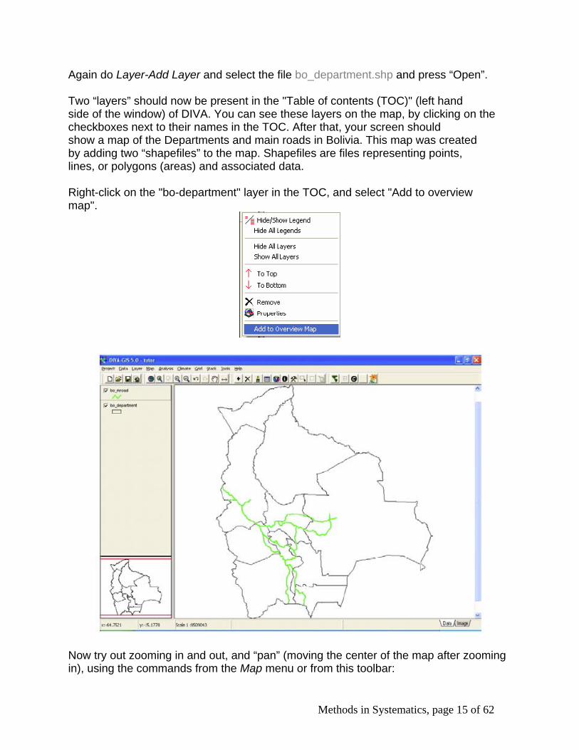
Open the file bolivia_wp.txt with Excel (or other spreadsheet program). Each record (row) in this file describes localities where wild potatoes have been collected.

First complete the LATITUDE and LONGITUDE columns by filling them with coordinate data in decimal degrees. Use the columns LATD, LATM, LATH, LOND, LONM, LONGH. LATD y LOND have degrees data, LATM y LONGM have decimal minutes (not minutes and seconds)), LATH and LONGH indicate the hemisphere (N/S and E/W). To calculate Latitude use a formula like “=-1*(LATD+LATM/60)” (but replace the variable names by the cell references in excel). The values in the first data row have already been calculated. It is important that in Excel you set the format of the cells to a certain number of decimals (e.g. 5). Otherwise, all the decimal numbers may be cut off when exporting the file. When you are done save the file under a different name. After that, save it as a TAB delimited text file again (.TXT).


Use Data/Points (text) to Shapefile to create a shapefile from the TXT file you just made with Excel. Select the TXT file as Input File, and for Longitude and Latitude select the columns LONGITUDE and LATITUDE. Click on Output file, Set the name of the output file to "bolivia_wp". Click Apply.

When the program finishes it will add the shapefile to the map. A layer showing locations where wild potatoes were collected in Bolivia should be shown. Your screen should look similar to this:


Now add a new layer "bol_alt.grd" to the map, rearrange the layers and zoom in to make a map like this:


This layer is made from a "gridfile", which is a different file type than the files previously used. It does not store features such as points, lines, or polygons, but rather it stores a rectangular raster (grid) of values. In this case, the values represent altitude (in meters above sea level). Make the bol_alt the active layer and move your mouse over the map. Note that you can see the values of the layer displayed on the status bar (the bottom of the window).


2. Data analysis Let’s make a new gridfile with the number of observations of wild potatoes in Bolivia. Make Bolivia_wp the active layer, and then click on Analysis – Point to Grid -Richness.

Go to the Parameters tab and select the field "Species".


Go back to the Options tab, choose an output filename and press Apply. When the program is finished, drag the bo_department layer to the top and change (in the Properties window) its Style to No fill. The map shows a grid that consists of five colors, each indicating a range of the number of species per grid cell.

When the grid is the active layer, the row and column number and the value of the cell are shown at the bottom of the screen, when moving the mouse over the map. To change the way the grid is displayed and show other ranges (e.g.,: 1-10, 10- 20, etc), or individual values, double click on the grid. The grid Properties window appears. Click on a value in the “To” column and change it. You can also insert more rows (ranges) using “Insert row” (+).


Make some more grids. First activate the bolivia_wp layer. Then select Analysis/Point to Grid/Richness. Select Define Grid-Options. In the Adjust With use Rows/Columns. Change the resolution (size) of the cells to 0.5 degrees and click OK. Then click Apply in the Create Grid window. The result is a grid with smaller cells than the previous grid (and hence with different values).

Make another grid using the same data, but now of the number of observations per grid cell. In Output Variable select Richness / Number of Observations.


Choose an output file name and click on Apply. Save your project (Project / Save).


DIVA-GIS: Distribution and Diversity of Wild Potatoes You should have gone through the tutorial and at least glanced through the manual before starting this exercise.

Wild potatoes (Solanaceae; Solanum sect. Petota) are relatives of the cultivated potato. There are nearly 200 different species that occur in the Americas. Their geographic distribution was recently described by Hijmans and Spooner (Hijmans, R.J., and D.M. Spooner, 2001. Geographic distribution of wild potato species. American Journal of Botany 88:2101-2112). In this exercise, we analyze some of the same data that were used in this paper.

A. Import data

1) Open the file ‘wildpot.txt’ with Excel to convert the data into decimal degrees (see Chapter 2 of the manual). Use both minutes and seconds information to do this. Save the file in tab delimited text format (as “wildpot-decimaled.txt”). Make sure that you do not lose the decimal numbers of the coordinates as you save the file.

2) Use this text file to make a shapefile called “wild potatoes”, save it in your folder and add it to the map. Also add the ‘pt_countries’ shapefile to the map.

In DESIGN, copy this image to the clipboard and pasted into a WORD

document. Label this figure “Fig. 1” along with a caption at the bottom of the figure. Save your WORD document as “471-potatoes-YOURNAME.doc”.

B. Summarize by country

3) We are first going to summarize the data by country. Make the potato shapefile the active file and click on Analysis/Point to Polygon (see figure below). Select ‘species’ as the field of interest. Add the shapefile of countries in the ‘define shape of polygon’ box. Select an output filename and press Apply.

The result is a new countries layer. Make this layer visible and the other two layers invisible. Double click on the new layer and change its legend attributes.


First, on the single tab, double click on the symbol and change its style to ‘solid fill’. Then go to the classes tab, select the “SPP” field, 6 classes, and reset the legend. SPP stands for the number of distinct species. Don’t worry about the other fields (however, the manual will give you this information).

Manually change the values (and colors) to of the different classes to get something like this below, where countries with no potato species are white, those with 1<10 are yellow, those with 10<20 are green, 20<30 are blue, 30<40 are purple, and >=40 are red.


Which country has the most species and with how many? ________________

Which country is second and with how many? ___________________

Which country is third and with how many? ___________________

Fourth? ___________________

Fifth? ___________________ Sixth? ___________________ Move the shapefile of wild potato collections to the top and, in design view, copy to the computer clipboard and pasted into your WORD document as figure 2, along with a legend. 4) If you open the table associated with the shapefile, you will see that there

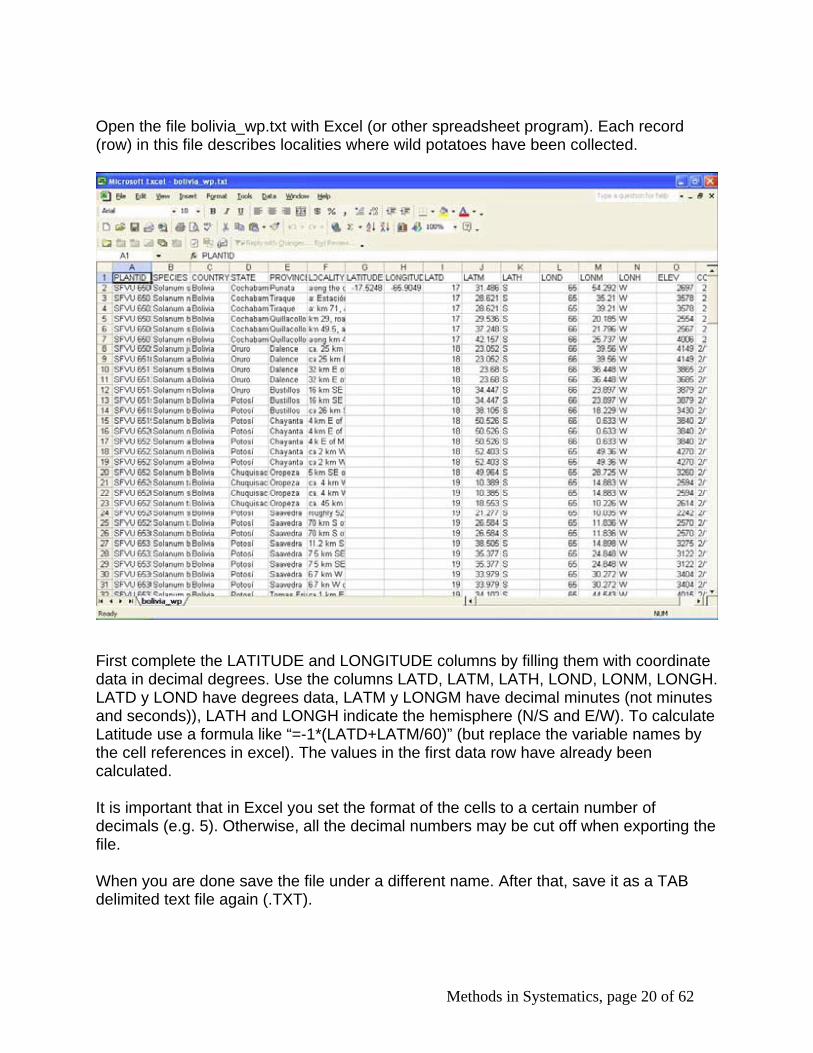
are records for many countries that have no potatoes at all. To simplify our table, we first select the records with more than 0 observations. Using Layer/Select Records and the select by query tab.

After entering the appropriate query all countries with potatoes will be colored yellow on the map (they are ‘selected’). Now save the selection to a new shapefile (“DATA>Selection to new shapefile”), add it to the map, and open the table. The table should look something like this:

The information by country is of interest and can be useful. However, it is not very helpful for understanding the spatial distribution of wild potatoes because the countries have such different sizes and shapes, and because most are very large. It is in most cases better to use grids with cells of equal area, and that is what we will do next.

Save the project to, e.g., ‘exercise1A’.


C. Project the data

To be able to use a grid with cells of equal area, the data needs to be projected. If the lat/long data were used, cells of say 1 square degree would get smaller as you move away from the equator: think of the meridians (vertical lines) on the globe getting closer to each other as you go towards the poles.

For small areas, UTM would be a good projection, but it this case we will use a projection that can be used for a complete hemisphere: the Lambert Equal Area Azimuthal projection. Before you project your data, you must choose a map origin for your data. This should be somewhere in the center of your points, to minimize the distance (and hence distortion) from any point to the origin. In this case, the center could be (-80, 0).

5) Remove all layers from the map, except the wild potato and the original country shapefile.

Project these files using Tools/Projection. Choose “projection of hemisphere”, then the “Lambert Equal Area Azimuthal (equatorial)” projection. On the custom tab, change the central meridian to -80. Save the files with filenames such as ‘wild potatoes lambert’ and ‘countries lambert’. Press Apply. Be patient…

Make all layers visible. If you zoom to the maximum extent (right click on data-map window, then “full extent), you see the projected data. Note that the shape of the countries is much more similar to their shape on a globe than before projecting. In the bottom left corner you can see that


the coordinate system has changed. You likely see very large numbers now: these express the distance from the origin (-80,0 degrees) in meters. If you make the projected potato file invisible, you will see that the unprojected data is still present on the map, near the origin of the projected data. Zoom in to that area.

Clearly one cannot combine projected and unprojected data (or data in two different projections) on a single map. Get rid of the old, unprojected data.

6) Now go to Map/Properties and change the projection to “Other” and the units to ‘meters’. This will allow for displaying a correct scale on the map.

7) Save the project to ‘Exercise 1B’.

D. Species Richness on a grid

8) Let’s determine the distribution of species richness (i.e., species per unit area) using a grid. This can be done using the point-to-polygon option that we used before, but in most cases it is more appropriate to use Analysis/Point to grid.

Select ‘Richness’ and ‘Number of different classes’, and select the ‘Species’ Field.

Create a new grid (call it “spp-richness grid”). In the Options window, set the X and Y dimensions of the cell size to 100,000 (as the projection is in meters this means that the cells will be 100 by 100 km). Use the default option (‘simple’) for the Point-to-grid procedure.

Choose an output filename (e.g., ‘species richness’, and press Apply). Play around


with the cell size (try 100 by 100 meters, 10,000 by 10,000, etc.). Return to 100,000 by 100,000.

9) Now make a grid of the ‘Number of observations’ instead of species richness.

(use the same procedure as above, but use the Richness subfield of “number of observations” rather than “distinct classes”). Define the new grid with the option ‘Use parameters from another grid’ and select the species richness grid you just made. In this way you assure that you use exactly the same grid (cell size, number of rows and columns, and geographic origin).

10) Compare the two grids with Analysis/Regression.

Is the number of species in a cell a function of the number of observations?

Copy an image of this graph and paste it into your WORD document. Email this to me and turn this handout with your answers marked onto it (5 pts.).

BIOL-471 – Methods in Systematics Spring 2007, Dr. Hardy


DIVA-GIS: Distribution and Diversity of Parks Herbarium Specimens (this plus a WORD document is to be handed in for 5 pts; work alone)

You should have gone through the tutorial and non-tutorial exercise 1 before starting this exercise.

A. Import data

1) Open DIVA-GIS.

2) Add data layers (here, shapefiles) for the following:

North American administrative boundaries (i.e., countries), US states, and US counties.

In the table of contents (left side in DIVA), rename these layers as above.

3) In Excel, open the file Parks-Herbarium-Jan-2007.xls, export (i.e., Save) this as a tab-delimited text file (Parks-Herbarium-Jan-2007.txt).

4) Open this file using DATA/Import points to shapefile. Double click on this layer and alter properties (take points to size 6, change

the color of the points to your liking). 5) Make the counties layer temporarily invisible. Zoom into the United States

and, in DESIGN view, copy this image to the clipboard and paste it into a WORD document. Label this figure “Fig. 1” along with a caption at the bottom of the figure. Save your WORD document as “Parks-Herbarium-Summary-YOURNAME.doc”.

6) Make the counties layer visible again.

B. Summarize by county

1. Make the Herbarium Specimen shapefile the active layer and click on Analysis/Point to Polygon. Select ‘Species’ as the field of interest. The program most likely mistakingly counted some blank cells as a species without a name (see figure next page)—unclick that such that we don’t count it. Also find “UNKNOWN” and unclick that. These are specimens for which species identity was not known. We do not want that.



Under the Options tab in the same box, add the shapefile of Counties in the ‘Define Shape of Polygon’ box. Select an output filename (“Summary-by-county.shp”; saved in your personal folder) and press Apply.

The result is a new layer that summarizes your specimen data by county. Make this layer the active layer (and make it visible if need be). Double click on the new layer and change its legend attributes.

First, on the single tab, double click on the symbol and change its style to ‘solid fill’. Then go to the classes tab, select the “SPP” field, 6 classes, and reset the legend. SPP stands for the number of distinct species.

Manually change the values (and colors) so that the different classes to get something like this below, where counties with no species are grey, those with 1<20 are yellow, those with 20<40 are green, 40<60 are blue, 60<80 are purple, and >=80 are red.

do not use “blank” cells or records for which the species was listed as “unknown” when summarizing records for each county.



Which county has the most species and with how many? ________________

How many collections are from this county (i.e., observations, abbreviated as OBS)? ____________________

Which county is second and with how many? ___________________


Which county is third and with how many? ___________________


Fourth? ___________________

Fifth? ___________________ Sixth? ___________________

Play around with the values in the classes table of this layer until you get the county with the most species to be the only red county.

Make sure that the Summary-by-county layer is on top. Then, in Design view, add a legend for this summary layer (one that will indicate the color-coding scheme. Then copy this image to the clipboard and paste it into your WORD document as Fig. 2 along with a figure caption.

Do you think that the number of species recorded from each county is correlated with the number of collections from that county? Back you answer with simple statistics, etc. __________________________________________

C. Summarize by state

Do the same for state as you did for counties. Play around with the classes values and produce a graphic of species per state, color-coded such that the state with the most species is red. Make a graphic and paste it into your WORD document as Fig. 3 with a caption.



Which state has the most species and with how many? ________________

How many collections are from this state? ____________________

Which state is second and with how many? ___________________


Which state is third and with how many? ___________________


Fourth? ___________________

Fifth? ___________________ Sixth? ___________________

PA is known to have about 3,200 plant species. How many are represented in our herbarium? What percent of the total flora is this?

__________________________________________

D. Produce a map showing the number of collections (i.e., observations or OBS) per county.

Color code this such that the top 5 counties in PA have their own color (in a graded series from yellow to red). Feel free to pick a threshold number of collections, below which the county is colored grey. Produce Figure 4 from this in your WORD document. Along with a caption. What are the top 5 PA counties in terms of collections and with how many? _______________________________________________________ Are the top 5 counties in PA in terms of collections the same as the top 5 in terms of observations? _________________ Do you think that the specimens you databased (which are not included here) would change the patterns you’ve seen? Why?

BIOL 471 – Methods in Systematics Prof. Hardy, Spring 2007


_______________________________________________________



Exercise 04: Georeferencing and Generating Distribution Maps Exercise Overview: Dr. Hardy will announce in class selected plant taxa that are well represented in our herbarium. Dr. Hardy has selected these to be more or less equal in size to one another (i.e., about 50 specimens). Please select one taxon (first come first serve) and then database all specimen sheets (using Microsoft Excel) and map each sheet as accurately as possible by assigning it the latitude / longitude in decimal degrees of the locality described on the label. Deliver via email both the Excel spreadsheet of all your specimens databased, plus a GEOLOCATE .xml file containing the map that GEOLOCATE generated for your data by the beginning of class on the specified data.

Objectives 1. For you to learn how a herbarium is organized and the types of important biogeographical data they contain. 2. For you to learn how to use Excel and issues in database management. 3. For you to learn about the developing field of biodiversity informatics and innovative georeferencing and mapping techniques. 3. For you to be aware of potential downstream applications of such a database. 4. For you to sleep at night dreaming of wonderfully pressed herbarium specimens and specimen labels that provide clear and detailed locality data. 5. (Long-term) For MU botany to learn a bit about the history of the flora of the Lower Susquehanna River Valley over the last ca. 150 years, by getting the complete collection databased and georeferenced to at least county-precision.

Instructions for databasing your specimens 1. To start, you must database your specimens using the Excel spreadsheet provided on our class website. 2. For any specimen, if species ID is unknown, but the genus is known, then indicate a “sp.” for “species” in the specific epithet field. 3. If “Collector” is unknown, indicate by “unknown”. 4. If Collector is known, yet there is no collection number, then indicate “s.n.” for collection number. This is a Latin abbreviation for “no number”. Thus, a James C. Parks collection with no number is “Parks, J. C.” followed by “s.n.” in the next column. 5. If you are unsure of any label information (i.e., the hand-writing is too difficult to read), then indicate so with your comments in a separate column at the far right of your spreadsheet. For example, “Carson Creek [Databaser is unsure about “Carson”]”. 6. Stamp your specimen sheet at the bottom left corner “COMPLETE” using stamps available in the herbarium.

Georeferencing using GEOLOCATE 1. I recommend georeferencing for each specimen individually; however, there are ways to enter all text locality information first, followed by automated batch georeferencing. The GEOLOCATE manual is available in the herbarium. 2. Open GeoLocate and, if necessary, “Georeference>Switch to user input”. 3. Enter all locality information for the specimen and hit “Georeference” to get latitude and longitude.



4. Check for accuracy. Verify every point. GEOLOCATE provides a way to edit (“correcting”) mapped points by clicking and dragging the point on the map to the correct local (read the manual). Hardcopy atlases are available in herbarium if necessary. If no specific locale is given, but you know the county or the state, then place cursor over that locale in the GEOLOCATE map viewer window and record the coordinates for the center point of that county or state. Indicate the level of accuracy. 5. Once all specimens have “lat” and “lon” down to at least the county-level, save your file from Excel as a “.csv” file (a special type of text file, via “FILE > Save as”). Mapping & Inserting electronic images of your GEOLOCATE maps into your MS WORD

document 1. In GEOLOCATE, open your “.csv” file for each taxon to be mapped (should do this separately). Although spreadsheets can include all taxa, it is necessary to make separately temporary “.csv” files for each taxon (only specimens for that taxon) for import into GEOLOCATE for mapping. MAKE SURE YOU KEEP THE ORIGINAL, COMPLETE FILE (I.E., WITH ALL SPECIES, ALL SPECIMENS GEOREFERENCED) FOR DELIVERY TO ME. 2. Map the specimens using “FILE > Plot all”. 3. Enlarge GEOLOCATE window to full screen. Keyboard the “shift + print screen” or simply “print screen” key combination to copy the screen to your clipboard, and then pasted into your MS WORD document. Format the picture in WORD (double click on the image to open relevant menu) to show only the map area (i.e., crop away anything else on the image). There are other ways to get images from the screen. But an explanation of these many ways is declined here. 4. Save your WORD document as a work in progress.

Instructions for final products 1. Send via email your final georeferenced spreadsheet (.xls or .csv format is fine). 2. Send via email a GEOLOCATE .XML file of your report. All of this by the beginning of class on February 14, 2007. These are together worth 20 points and will be graded based on completeness (8 pts), quality, and accuracy (12 pts). **************************************************************************** Groups to do.... 1-6. Sunflower Family (Compositae or Asteraceae)

1. A-C – Aster 2. Ambrosia – Cichorium 3. Chrysanthemum – Erigeron

4. Eupatorium – Hieracium 5. Inula – Siphium 6. Silybum – the end

7. Coffee & Quinine Family (Rubiaceae) 8. Violet Family (Violaceae)



Exercise 05: DIVA-GIS: Biogeographic (Distribution) Modeling using Herbarium Specimens and Climate Data

(this plus a WORD document is to be handed in for 10 pts; work alone)

A. Import and view data.

1) Open DIVA-GIS.

2) Add data layers (here, shapefiles) for the following:

North American administrative boundaries (i.e., countries), US states, and US counties.

In the table of contents (left side in DIVA), rename these layers as above.

3) In Excel, open your GEOLOCATED Excel file. Make sure that there is a header row, with Latitude (or Lat) and Longitute (or Lon) marked in particular. Export (i.e., Save) this as a tab-delimited text file with a .txt extension.

4) Open this file using DATA>Import points to shapefile. Double click on this layer and alter properties (take points to size 6, change

the color of the points to your liking). 5) To save this file with ALL SUPPORTING DATA SUCH THAT YOU CAN OPEN IT ON

ANY COMPUTER, export DIVA file as follows:

B. Determine the genus with the most specimens.

1. What is the genus with largest number of specimens? ______________

How many specimens are mapped? ________________

2. Using LAYER>Select Records, select and highlight only the records for this genus. These points on the map will now be yellow.

3. Using DATA>Selection to New Shapefile, make a new layer (shapefile) with only the points for this genus. Name the new layer/shapefile accordingly.

4. Make the original layer with ALL specimens invisible.



C. Model the distribution of your genus.

1. With the new genus layer active and using the menu option MODELING>Bioclim/Domain, open the following window:

2. Select the “Predict” tab on the far right of this window to bring up the following window:

You will be using the climate data contained in “worldclim_10m.clm”, which has climate data (temperature, rainfall, etc.) at the resolution of 10 geospatial minutes. How many degrees does this represent? ___________ How many degrees wide is PA? ____________ Therefore, to what resolution should you be able to model the actual range of your genus?



3. In the window below, clear all climatic variables except for maximum and minimum temperature and average maximum and minimum precipitation. Save output gridfile as “GENUS-YOURNAME-prediction01.grd”. Click APPLY. You’ve just predicted the possible range for this genus based on these climatic variables.

The default is to make a range prediction restricted to a bounding box defined by the geographical limits of your specimen records. However, use this button, followed by click-and-dragging the mouse to define a rectangle encompassing all of North America (and only N America) north of Mexico. DO NOT yet press “Apply”.





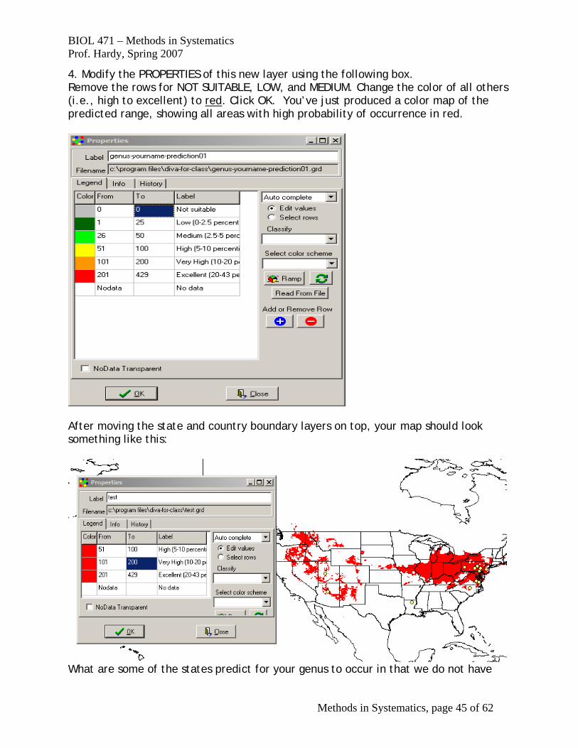
4. Modify the PROPERTIES of this new layer using the following box. Remove the rows for NOT SUITABLE, LOW, and MEDIUM. Change the color of all others (i.e., high to excellent) to red. Click OK. You’ve just produced a color map of the predicted range, showing all areas with high probability of occurrence in red.

After moving the state and country boundary layers on top, your map should look something like this:

What are some of the states predict for your genus to occur in that we do not have



records for in our herbarium? 5. Now, with the original “genus” layer active, do steps C1-C4 again, only this time use ALL CLIMATIC VARIABLES, and make the predicted High probability range blue. Name this new layer appropriately. Is the distribution predicted now larger, smaller, or about the same area as that the first time around? ________________________________ Is this expected? ________________________________ Copy an image of this map (showing all herbarium specimens for the genus, plus the two predicted ranges and all state and country boundaries, but not county boundaries) to a word document. Name it figure 1, along with an appropriate caption. 6. Zoom in to PA. Make the county boundaries layer visible again. Based on the climate predictions made using all climatic variables, what counties is your genus predicted to occur in for which we do not currently have specimens? _________________________________________________________________ Copy an image of the prediction for PA only to your WORD document. Name it Figure 2, along with caption. Of what use is this distribution modeling? Describe some of the limitations of our predicted ranges?



Phylogenetic Inference



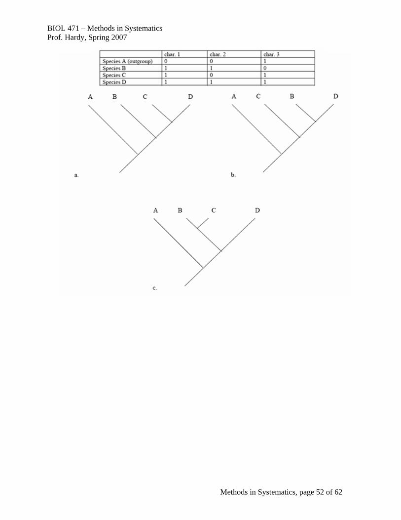
Simple, Manual Cladogram Construction 1. We wish to infer relationships among the major groups of vertebrates. 2. In order to “root” the phylogenetic hypothesis (i.e., our cladogram), we will choose the snail as the sole member of our outgroup. 3. Below is a character-by-taxon matrix for seven characters and their states.

Character and Character State List: 0. VERTEBRAE PRESENCE: no (0); yes (1). 1. LEGS PRESENCE: absent (0); present (1). 2. ENDOTHERMY: absent or cold-blooded (0); present or warm-blooded (1) 3. FUR PRESENCE: absent (0); present (1). 4. MAMMARY GLANDS PRESENCE: absent (0); present (1). 5. THUMB (OPPOSABILITY): not opposable (0); partially or fully opposable (1). 6. TAIL PRESENCE: present (0); absent (1).

4. In order to infer phylogeny, we will use the outgroup with the assumption that character states possessed by the outgroup are plesiomorphic.

States shared amongst members of ingroup (vetebrates) and the outrgoup (snails) are symplesiomorphies (i.e., shared plesiomorphies) and are not basis for identifying clades. Only synapomorphies (i.e., shared derived characteristics) point to clades or monophyletic groups.

5. ON THE NEXT PAGE: With each character treated separately, draw the cladogram suggested by each character. Use the principal of parsimony. When a character is uninformative with respective to certain relationships, draw those lineages as members of a polytomy (as opposed to dichotomy).

VERTEBRAE LEGS ENDOTHERMY FUR MAMMARY GLANDS

OPPOSABLE THUMB

TAIL

Snail 0 0 0 0 0 - - Fish 1 0 0 0 0 - 1 Lizard 1 1 0 0 0 0 1 Bird 1 1 1 0 0 0 1 Cow 1 1 1 1 1 0 1 Monkey 1 1 1 1 1 1 1 Gorilla 1 1 1 1 1 1 0 Human 1 1 1 1 1 1 0



Fish Lizard Bird Cow Monkey Gorilla Human








VERTEBRAE (0 > 1)

THUMB (0 > 1)

LEGS

ENDOTHERMY

FUR

MAMMARY

TAIL summary - final



6. Now add two characters – WING PRESENCE (absent = 0; present = 1) and PEDALITY (quadrupedal = 0; bipedal = 1).

7. Map and label these two new characters as hashmarks onto your summary tree. 8. Answer the following questions: Is the presence of wings informative with regards to relationships in our cladogram? Which kind(s) of inferred character transformation(s) is the origin of wings? (i.e., symplesiomorphy, synapomorphy, autapomorphy, apomorphy, and/or plesiomorphy) Is the presence of bipedality a synapomorphy in our cladogram? What is (are) the term(s) from lecture or your reading that would apply to this?

VERTEBRAE LEGS ENDOTHERMY FUR MAMMARY GLANDS

OPPOSABLE THUMB

TAIL WINGS PEDALITY

Snail 0 0 0 0 0 - - - - Fish 1 0 0 0 0 - 1 - - Lizard 1 1 0 0 0 0 1 0 0 Bird 1 1 1 0 0 0 1 1 1 Cow 1 1 1 1 1 0 1 0 0 Monkey 1 1 1 1 1 1 1 0 0 Gorilla 1 1 1 1 1 1 0 0 0 Human 1 1 1 1 1 1 0 0 1



Exercise 02: Character State Optimization for Choosing Most Parsimonious Cladograms and Reconstructing Ancestral States.

The method we will use here is called Fitch Optimization. The required reading for this is Fitch (1971). 1. Score terminal species for character of interest. Downward Pass 2. Starting at the tips of the cladogram, start with two sister species and assign the intersection or union of the two to the node below them. An intersection is where both descendants of the ancestral node have the same state; therefore, that state is assigned to the ancestral node. A union is where the two descendants of the ancestral node have different states; therefore, both are temporarily assigned to the node. 3. Work the same way from another pair of taxa, down the tree until all nodes have been assigned an intersection or union. [COUNT THE NUMBER OF UNIONS after the downpass, this is the most parsimonious length of that character on the cladogram.] Upward pass 4. Moving up the tree from the basal-most node (for simplicity-sake, assume that the state possessed by the most distant outgroup taxon is the state at the basal-most node), resolve any unions based upon the intersection with the lower node. If there is not intersection for a particular node on the up-pass, then your data are ambiguous for that node. [THE STATES ASSIGNED TO NODES are one (not necessarily the only one) most parsimonious reconstruction of the state possessed by the hypothetical ancestor of that node’s immediate descendants.] Now apply your method to determine (1) which is the most parsimonious tree on the next page and (2) the states for each character for each hypothetical ancestor in each tree.





Exercise 03: Morphological Datamatrix Construction and Basic Cladistic Analysis 1. Download WINCLADA (program 1) and NONA (program 2) from course website. 2. Save these to the My Documents “T” drive under our class folder in a subfolder called “Winclada”. 3. Change the file extension from .txt to .exe 4. Open WINCLADA and set the path to NONA as explained in the WINCLADA manual. Now you are ready for data matrix construction and analysis. 5. Construct a data matrix in WINCLADA exactly like the one handed out last time (reproduced below).

6. Run a simple analysis, as described under the “II. ANALYZING DATA > A. Heuristics” section of the WINCLADA manual. 7. How many trees are returned as most parsimonious? How many “steps” is this tree(s) (check the number of steps in the lower left hand corner of the screen in tree-viewing mode; if “L=10” then your tree has a length of 10, which is 10 steps)? Is it the same tree(s) that you found to be most parsimonious manually out of the possibilities below? Draw the tree(s) as it appears on your computer monitor and match it to one of the ones shown below.



8. Play around with tree styles as described in the WINCLADA manual (p. 22-23). 9. Trace (or map) your characters from the matrix onto your tree (see manual p. 23-24). Are they all there? 10. Now build a new matrix which is a copy of your vertebrate / tetrapod matrix from the other day.

11. Run an analysis. Print out the resulting tree. Is it the same as your summary tree from the last exercise? How many steps is this? 12. Add the two characters WINGS and BIPEDALISM. See WINCLADA manual for instructions. Rerun the analaysis. Do you find the same tree? How many steps is this one? 13. Add 10 autapomorphies to Birds (just make them up). Does this change the tree? Does cladistics group things based upon overall similarity or some special similarities? What are these special similarities called? You know the term.



Exercise 04: Use of DNA Sequences for Phylogenetic Inference. Since last class, you were to construct a matrix ready to be read by WINCLADA. This matrix included COX1 sequences for each of the following species: Conus textile (marine snail) Oncorhynchus mykiss (rainbow trout) Andrias japonicus (Japanese giant salamader) Lepidophyma flavimaculatum (night lizard) Struthio camelus (ostrich) Bos taurus (cow) Macaca mulatta (rhesus monkey) Homo sapiens Pan paniscus (chimp) Alligator mississippiensis (American alligator) To open this in WINCLADA, you had to follow the instructions handed out last time, and refer to the WINCLADA manual. Today, you need to open the matrix in WINCLADA and do the following: 1. Open WINCLADA. Change to color-coded states (VIEW>Color coded states). 2. Manually align this protein coding gene using ANALYZE>Moleculoid>Manual insert-delete. Use insert and delete buttons as in your manual to insert gaps to align sequences. 3. SAVE. 4. Run analysis, record the number of most parsimonious trees obtained, along with the length of that(those) trees. Print one out. Hand it in. NOW TODAY: You start a project (20 pts), were you must pick a group represented above, but expand upon it by increasing the sampling around the given species. Add ten more species. If you chose lizards, then attempt to get a broad taxonomic sampling of lizards by including presumed “primitive” and “advanced” members. You should consult taxonomic literature for that group. You are to hand this in at the beginning of class April 16, along with a 5-page (double-spaced) typed report on the clades you discover and some of their defining characteristics. Tables, Figures, and Literature cited section not included in the 5-page count. You are to hand this in at the beginning of class April 16, along with a 2-page (double-spaced) typed report on the clades you discover and some of their defining characteristics.



GRADING (20 pts total): Data matrix (1.5 pt) electronic submission to [email protected]) -alignment -spelling of species (binomial and common names must be included for each sequence). Stick GENBANK accession numbers in table of report, not in species names as appearing in your matrix. -completeness of data matrix Report: 1. Figure 1. (2 pt; can have more figures, but the resulting most parsimonious cladogram or strict consensus tree is the minimum). Goes in the “Results and Discussion” section. 2. Table 1. (2 pt; a list of the species represented along with their GENBANK accession numbers). This should go in the methods section. 3. Writing: -title (0.5 pt) -“Introduction” ( 2 pt) Background on your ingroup and the outgroup. Objectives of your investigation. No more than 1 page. -“Methods” (1 pt) Brief mention of programs used, the gene used, and source of sequences – GENBANK. No more than 1 page. -“Results and Discussion” (8 pt for writing component only) one combined section that presents the trees and discusses them and the clades they reveal. This is where you should also discuss morphological/anatomical characters that support each clade). -“Literature Cited” (3 pt) Complete list of all references cited in your report, using the format of Systematic Biology. Absolutely no websites.



Species



Exercise 01: Species Delimitation using Population Aggregation Analysis Required Reading: Davis, JI, KC Nixon. 1992. Populations, genetic variation, and the delimitation of phylogenetic species. Systematic Biology 41: 421-435. Below are data matrices that report the occurrence of 10 attributes from seven separate populations. How many species do these populations represent (the minimum number would be 1, the maximum would be 7)? Population 1 Attribute 1 2 3 4 5 6 7 8 9 10 Indiv. 1 1 0 0 0 1 0 0 0 1 1 Indiv. 2 1 1 0 0 1 1 1 0 1 1 Indiv. 3 1 1 0 0 1 1 0 0 0 1 Indiv. 4 1 1 0 0 1 1 1 0 1 1 Indiv. 5 1 0 0 0 0 1 0 1 1 1 Pop 1 profile

Population 2 Attribute 1 2 3 4 5 6 7 8 9 10 Indiv. 1 1 0 0 0 1 0 0 0 1 1 Indiv. 2 0 1 0 0 1 1 1 0 1 1 Indiv. 3 1 0 0 1 1 1 0 0 0 1 Indiv. 4 1 0 0 1 1 1 1 0 1 1 Indiv. 5 1 0 0 0 0 1 0 1 1 1 Pop 2 profile

How many putative species do we have after 2 populations were profiled for 10 attributes? List the population-members of each species.




How many putative species do we have after 3 populations were profiled for 10 attributes? List the population-members of each species. Population 4 Attribute 1 2 3 4 5 6 7 8 9 10 Indiv. 1 1 0 0 0 1 0 0 0 1 1 Indiv. 2 0 1 0 0 1 1 1 0 1 1 Indiv. 3 1 0 0 1 1 1 0 0 0 1 Indiv. 4 1 0 0 1 1 1 1 0 1 1 Indiv. 5 1 0 0 0 0 1 0 1 1 1 Pop 4 profile


How many putative species do we have after 5 populations were profiled for 10 attributes? List the population-members of each species.





How many phylogenetic species do we in total, based upon this analysis? List the population-members of each species. What, if anything, could decrease the number of species recognized here? What, if anything, might increase the number of species recognized here?



Exercise 02: DNA in Species Delimitation, Diagnostics, and Conservation Forensics The project is as follows: 15 points total. Consult your WINCLADA manual or past lecture or assignment materials for help with the following procedure. 1. Build a fasta format text file with GENBANK mitochondrial cytochrome b (abbreviated as Cytb) sequences from the following sturgeons used for caviar. Partial sequences are okay. NOTE: the species indicated by an asterisk provide high priced caviar much sought after. The species with two asterisks (**) is an Atlantic species listed as endangered by the US Fish and Wildlife service and is therefore illegal to collect for caviar. *Sevruga sturgeon (Acipenser stellatus) Persian sturgeon (A. persicus) Adriatic sturgeon (A. naccariu) Siberian sturgeon (A. baerii) *Ossetra sturgean (A. gueldenstaedtii) Ship sturgeon (A. nudiventris) *Belgua (Huso huso) American paddlefish (Polyodon spathula) Amur River sturgeon (A. schrenckii) White sturgeon (A. transmontanus) Eastern beluga (Huso dauricus) **Shortnose sturgeon (Acipenser brevirostrum) 2. Align these sequences (you may use CLUSTAL, but you must tweak the alignment parameters to get a good alignment, and then import into WINCLADA for adjustment) 3. Run a cladistic analysis (root with Polyodon spathula) and determine the identity of unknown caviar collected from New York markets last week by your instructor. 4. Identify diagnostic base positions (positions in their genes, based on your alignment) for each species. For example, you might refer to your cladogram and a diagnostic base position to support your conclusion regarding the identity of your unknown (“Based on the cladistic analysis (Fig. 1) and a diagnostic “A” at position 26 and “T” at position 30, the known sample is actually the Persian sturgeon (Acipenser persicus). Thus, our sample was actually mislabeled at the market it was collected from.”) 4. Save all materials often and email files to yourself (or save them on removable disk of your own). 5. Write a two page report (figures not included) on the identity of the unknown assigned to you. Be sure to include a brief description of your methods and figures such as strict consensus



cladograms, etc. Hand this plus your aligned WINCLADA matrix in by 6 pm Monday April 30. Earlier if possible. email matrix to [email protected]