Exergy Analysis of a Ground-Source Heat Pump … Analysis of a Ground-Source Heat Pump System Kathrin Menberg1,2, Yeonsook Heo2, Wonjun Choi 3, Ryozo Ooka , Ruchi Choudhary1, Masanori

Proceedings of the 15th IBPSA ConferenceSan Francisco, CA, USA, Aug. 7-9, 2017

1646https://doi.org/10.26868/25222708.2017.437

Exergy Analysis of a Ground-Source Heat Pump System

Kathrin Menberg1,2, Yeonsook Heo2, Wonjun Choi3, Ryozo Ooka3, Ruchi Choudhary1, Masanori

Shukuya4 1 University of Cambridge, Department of Engineering, Cambridge, UK, 2 University of Cambridge, Department of Architecture, Cambridge, UK,

3 University of Tokyo, Institute of Industrial Science, Tokyo, Japan, 4 Tokyo City University, Department of Restoration Ecology and Built Environment, Tokyo, Japan

Abstract

In contrast to energy analysis, the analysis of exergy al-

lows the evaluation of the quality of different energy

flows and enables a comprehensive assessment of the per-formance of a system and its individual components by

accounting for necessary exergy consumption and unnec-

essary consumption. While exergy analysis methods have

been applied to a variety of conventional and renewable

energy supply systems, there is still a lack of knowledge

regarding the detailed exergy flows and exergy efficien-

cies of ground-source heat pump systems (GSHP).

In this study, we develop a thermodynamic model for a

ground-sourced cooling system of an existing building by

applying the concept of cool and warm exergy. In addi-

tion, we investigate the effect of varying temperature con-

ditions, such as reference and ground temperatures, on the exergy flows and system performance.

Introduction

In thermodynamics, the exergy content of a system is de-

fined as the maximum theoretical amount of work that can

be extracted from the system in relation to a certain refer-

ence state. The analysis of exergy contents and flows of-

fers a concept to assess the quality of energy, which has

hitherto been applied in various fields of engineering and

science (Li et al., 2014).

Energy analysis methods, which are based on the princi-

ple of energy conservation, are often inadequate for gain-

ing a full understanding of all important aspects of energy utilisation in energy supply systems (Schmidt, 2009). The

analysis of exergy on the other hand allows evaluation of

the quality of energy flows through individual compo-

nents of an energy supply system and thus enables a lo-

calised assessment of subsystem efficiencies. As a result,

the magnitude and location of thermodynamic inefficien-

cies can be pinpointed and options for system improve-

ment can be identified.

The large potential of exergy analysis with regard to per-

formance evaluation has led to an increasing number of

studies applying these methods to a large variety of en-

ergy supply systems. However, most of these studies re-gard exergy consumption of lumped subsystem compo-

nents, such as the distribution system, heating system or

the building envelope (Schmidt, 2009; Kazanci, 2016). So

far, few studies have evaluated the exergy performance of

the different components of a GSHP system in detail (Li

et al., 2014). While some studies evaluated the effect of

varying reference, i.e. outdoor, conditions on the overall

exergy performance of an energy supply system (Zhou &

Gong, 2013), there is still a lack of knowledge regarding sub-system components. In addition, a detailed thermody-

namic model consisting of a number of sub-system com-

ponents often operates under various temperature bound-

ary conditions, such as ground and indoor temperature,

which might have very diverse effects on the exergy per-

formance.

In this study, we analyse the exergy performance of a

GSHP system with a radiant ceiling. We do so by apply-

ing the concept of warm and cool exergy to the thermo-

dynamic model of the system. The model includes formu-

lations for the energy and exergy terms for all individual

subsystems, such as the heat pump, mixing valve and the radiant ceiling, which allows an in-depth analysis of the

exergy flows and consumption for each subsystem. As

tools for exergy analysis of energy systems are currently

not incorporated in common building simulation pack-

ages, such as TRNSYS or EnergyPlus, the formulation of

our model also comprises a first step towards introducing

exergy analysis to the transient building simulation frame-

work and adds to the promotion of exergy analyses within

existing energy simulation tools.

In addition, we assess the effect that variations in the

boundary conditions, such as reference and ground tem-perature, and internal system temperatures (such as the

temperature difference between inlet and outlet flow),

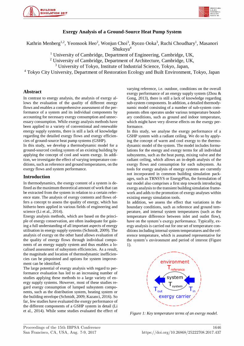
have on the system’s exergy performance. Typically, ex-

ergy analysis is carried out for one set of temperature con-

ditions including internal system temperatures and the ref-

erence temperature, which is assumed representative for

the system’s environment and period of interest (Figure

1).

Figure 1: Key temperature terms of an exergy model.


1647

As energy supply systems provide indoor heating and

cooling with respect to the outdoor conditions, the out-

door ambient air temperature is the most obvious choice

for the reference temperature. Accordingly, all exergy

contents or consumptions are quantified with respect to

the outdoor thermal state, which will directly influence

the magnitude of the exergy values. The individual impact

of the reference and system temperatures on exergy out-

put and consumption are evaluated per component by as-

signing parametric temperature changes. To quantify the

magnitude of the overall effect and identify those temper-ature parameters that have the most significant influence

on the overall exergy performance, we conduct a sensitiv-

ity analysis using Morris method.

Methodology

Exergy analysis

According to Shukuya (2013) exergy is defined as a meas-

ure for the dispersion potential of energy, while entropy

is a measure for this dispersion of energy. Furthermore,

exergy can be considered as warm or cool exergy, depend-

ing on the system temperature T and the reference temper-

ature T0. If the system temperature T is higher than T0, the

thermal energy Q contained in the system can disperse into the environment, which acts as a cold reservoir, as a

flow of warm exergy (eq. 1). If the environment is warmer

than the system, exergy in form of cool exergy can flow

out of the system into the environment, denoting the lack

of thermal energy by (-Q*) (eq. 2) (Shukuya, 2013).

𝑋𝑤𝑎𝑟𝑚 = (1 − 𝑇0

𝑇) 𝑄, 𝑓𝑜𝑟 𝑇 > 𝑇0 (1)

𝑋𝑐𝑜𝑜𝑙 = (1 − 𝑇0

𝑇) (−𝑄∗), 𝑓𝑜𝑟 𝑇0 > 𝑇 (2)

For any system under consideration, one can obtain the

general energy balance equation according to the princi-

ple of energy conservation.

[𝑒𝑛𝑒𝑟𝑔𝑦 𝑖𝑛𝑝𝑢𝑡] = [𝑒𝑛𝑒𝑟𝑔𝑦 𝑠𝑡𝑜𝑟𝑒𝑑]+ [𝑒𝑛𝑒𝑟𝑔𝑦 𝑜𝑢𝑡𝑝𝑢𝑡]

(3)

Furthermore, because of the relation of energy and en-

tropy (eq. 4a), a general exergy balance equation for any system can be written as eq. 4b (Li et al., 2014).

𝑒𝑥𝑒𝑟𝑔𝑦 = 𝑒𝑛𝑒𝑟𝑔𝑦 − 𝑒𝑛𝑡𝑟𝑜𝑝𝑦 ∙ 𝑇0 (4a)

[𝑒𝑥𝑒𝑟𝑔𝑦 𝑖𝑛𝑝𝑢𝑡] − [𝑒𝑥𝑒𝑟𝑔𝑦 𝑐𝑜𝑛𝑠𝑢𝑚𝑒𝑑] = [𝑒𝑥𝑒𝑟𝑔𝑦 𝑠𝑡𝑜𝑟𝑒𝑑] + [𝑒𝑥𝑒𝑟𝑔𝑦 𝑜𝑢𝑡𝑝𝑢𝑡]

(4b)

These equations state that the exergy inputs into any sys-

tem or component, such as the exergy contained in fluids

that enter the system, minus the exergy consumed during

heat transfer in that system, are equal to the sum of exergy

outputs, such as cool exergy delivered to a room or exergy

contained in outlet flow.

System overview

The GSHP system used as a case study for the exergy

analysis is installed in the Architecture Studio Building at

the University of Cambridge and supplies cooling for a

large open office space. It consists of two vertical bore-

hole heat exchangers (BHEs) and a reversible brine-to-

water heat pump (HP). Thermal energy is supplied to (or

extracted from) the room by radiant ceiling panels.

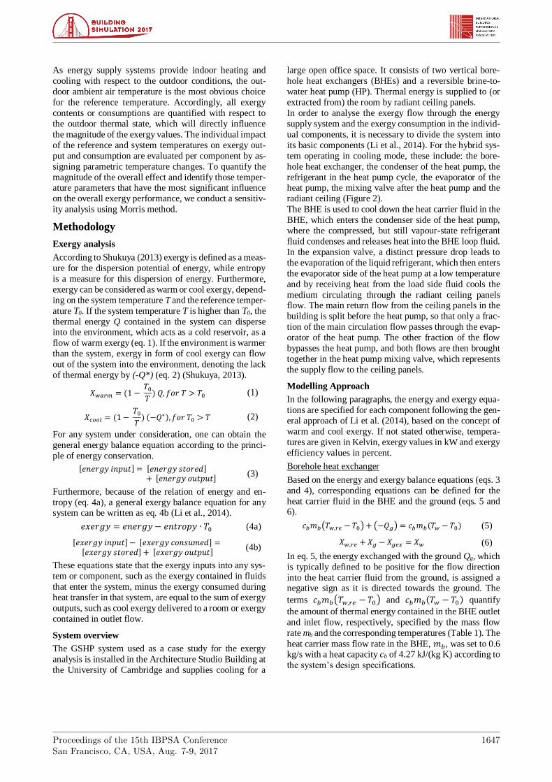
In order to analyse the exergy flow through the energy

supply system and the exergy consumption in the individ-

ual components, it is necessary to divide the system into

its basic components (Li et al., 2014). For the hybrid sys-

tem operating in cooling mode, these include: the bore-

hole heat exchanger, the condenser of the heat pump, the

refrigerant in the heat pump cycle, the evaporator of the heat pump, the mixing valve after the heat pump and the

radiant ceiling (Figure 2).

The BHE is used to cool down the heat carrier fluid in the

BHE, which enters the condenser side of the heat pump,

where the compressed, but still vapour-state refrigerant

fluid condenses and releases heat into the BHE loop fluid.

In the expansion valve, a distinct pressure drop leads to

the evaporation of the liquid refrigerant, which then enters

the evaporator side of the heat pump at a low temperature

and by receiving heat from the load side fluid cools the

medium circulating through the radiant ceiling panels flow. The main return flow from the ceiling panels in the

building is split before the heat pump, so that only a frac-

tion of the main circulation flow passes through the evap-

orator of the heat pump. The other fraction of the flow

bypasses the heat pump, and both flows are then brought

together in the heat pump mixing valve, which represents

the supply flow to the ceiling panels.

Modelling Approach

In the following paragraphs, the energy and exergy equa-

tions are specified for each component following the gen-

eral approach of Li et al. (2014), based on the concept of

warm and cool exergy. If not stated otherwise, tempera-

tures are given in Kelvin, exergy values in kW and exergy

efficiency values in percent.

Borehole heat exchanger

Based on the energy and exergy balance equations (eqs. 3

and 4), corresponding equations can be defined for the

heat carrier fluid in the BHE and the ground (eqs. 5 and 6).

𝑐𝑏𝑚𝑏(𝑇𝑤,𝑟𝑒 − 𝑇0) + (−𝑄𝑔) = 𝑐𝑏𝑚𝑏(𝑇𝑤 − 𝑇0) (5)

𝑋𝑤,𝑟𝑒 + 𝑋𝑔 − 𝑋𝑔𝑒𝑥 = 𝑋𝑤 (6)

In eq. 5, the energy exchanged with the ground Qg, which

is typically defined to be positive for the flow direction

into the heat carrier fluid from the ground, is assigned a negative sign as it is directed towards the ground. The

terms 𝑐𝑏𝑚𝑏(𝑇𝑤,𝑟𝑒 − 𝑇0) and 𝑐𝑏𝑚𝑏(𝑇𝑤 − 𝑇0) quantify

the amount of thermal energy contained in the BHE outlet

and inlet flow, respectively, specified by the mass flow

rate mb and the corresponding temperatures (Table 1). The

heat carrier mass flow rate in the BHE, 𝑚𝑏, was set to 0.6 kg/s with a heat capacity cb of 4.27 kJ/(kg K) according to

the system’s design specifications.


1648

Figure 2: Individual components of the GSHP system with the energy, exergy and temperature terms applying to the

corresponding components.

In eq. 6, the exergy extracted from the ground Xg com-

prises cool exergy, as the internal sub-system temperature

Tg is lower than the reference temperature T0 outside of the system, and can be defined according to eq. 7. Xw,re is

the exergy of the heat carrier fluid return flow (eq. 8),

while Xgex is the exergy consumption during heat ex-

change with the ground, and Xw is the output exergy com-

prised in the BHE outlet flow (eq. 9).

𝑋𝑔 = (1 −𝑇0

𝑇𝑔) (−𝑄𝑔) (7)

𝑋𝑤,𝑟𝑒 = 𝑐𝑏𝑚𝑏 {(𝑇𝑤,𝑟𝑒 − 𝑇0) − 𝑇0 𝑙𝑛𝑇𝑤,𝑟𝑒

𝑇0} (8)

𝑋𝑤 = 𝑐𝑏𝑚𝑏 {(𝑇𝑤 − 𝑇0) − 𝑇0 𝑙𝑛𝑇𝑤

𝑇0}

(9)

Condenser of the heat pump

The energy and exergy balances of the condenser within

the heat pump are given in eqs. 10 and 11, which also con-

sider the electricity to drive the ground loop pump Epump

(0.38 kW) as an energy input. Eq. 11 has two input terms, Xw and Epump, as well as two output terms, Xw,re and Xc,

which represents the exergy output into the refrigerant

(eq. 12). Xcond quantifies the exergy consumption in the

condenser.

𝐸𝑝𝑢𝑚𝑝 + 𝑐𝑏𝑚𝑏(𝑇𝑤 − 𝑇0) = 𝑐𝑏𝑚𝑏(𝑇𝑤,𝑟𝑒 − 𝑇0) +(−𝑄𝑐)

(10)

𝐸𝑝𝑢𝑚𝑝 + 𝑋𝑤 − 𝑋𝑐𝑜𝑛𝑑 = 𝑋𝑤,𝑟𝑒 + 𝑋𝑐 (11)

𝑋𝑐 = (1 −𝑇0

𝑇𝑐) (−𝑄𝑐) (12)

Refrigerant cycle

The energy and exergy balance equations (eq. 13, 14) of

the refrigerant loop in the heat pump can be defined based

on the according input (Qe, Xe) and output (Qc, Xc) terms

and accounting for the electricity demand of the compres-

sor Ecomp (1.25 kW) and the exergy consumption in the refrigerant cycle Xrefcycle.

𝐸𝑐𝑜𝑚𝑝 + 𝑄𝑒 = 𝑄𝑐 (13)

𝐸𝑐𝑜𝑚𝑝 + 𝑋𝑐−𝑋𝑟𝑒𝑓𝑐𝑦𝑐𝑙𝑒 = 𝑋𝑒 (14)

Evaporator of the heat pump

The energy balance of the evaporator side of the heat

pump in cooling mode is specified by eq. 15 and takes into

account the thermal energy content of the inlet and outlet

flow mHP of the heat pump load side and the power con-

sumption of the main circulation pump ECP (0.63 kW).

The heat capacity of the load side fluid cw was assumed to be 4.19 kJ/(kg K). The corresponding exergy balance (eq.

16) has three input terms: ECP, the exergy input from the

refrigerant at the evaporator Xe (eq. 17), and the exergy

content of the inlet flow XHP,in (eq. 18). The exergy of the

load side outlet flow XHP represents the exergy output of

the component (eq. 19), and the exergy consumption in

the evaporator is denoted by Xevap.

𝐸𝐶𝑝 + (−𝑄𝑒) + 𝑐𝑤𝑚𝐻𝑃(𝑇𝑟𝑒 − 𝑇0)

= 𝑐𝑤𝑚𝐻𝑃(𝑇𝐻𝑃 − 𝑇0) (15)

𝐸𝐶𝑃 + 𝑋𝑒 + 𝑋𝐻𝑃,𝑖𝑛 − 𝑋𝑒𝑣𝑎𝑝 = 𝑋𝐻𝑃 (16)

𝑋𝑒 = (1 −𝑇0

𝑇𝑒) (−𝑄𝑒) (17)

𝑋𝐻𝑃,𝑖𝑛 = 𝑐𝑤𝑚𝐻𝑃 {(𝑇𝑟𝑒 − 𝑇0) − 𝑇0 𝑙𝑛𝑇𝑟𝑒

𝑇0} (18)

𝑋𝐻𝑃 = 𝑐𝑤𝑚𝐻𝑃 {(𝑇𝐻𝑃 − 𝑇0) − 𝑇0 𝑙𝑛𝑇𝐻𝑃

𝑇0} (19)

Mixing valve after the heat pump

The energy balance for the HP mixing valve, where the

flow through the HP, mHP, is combined with the diverted

flow that bypasses the heat pump, mdivHP, is defined by the

contents of thermal energy of the two inlet flows and the

outlet flow mCP (eq. 20). The exergy balance (eq. 21) is

formed of the corresponding exergy contents of the inlet,

XHP (eq. 19) and XdivHP (eq. 22), and outlet flows Xsup (eq.

23), and an exergy consumption term XvalHP, which ac-counts for entropy generated during the mixing process.

𝑐𝑤𝑚𝐻𝑃(𝑇𝐻𝑃 − 𝑇0) + 𝑐𝑤𝑚𝑑𝑖𝑣𝐻𝑃(𝑇𝑟𝑒 − 𝑇0)

= 𝑐𝑤𝑚𝐶𝑃(𝑇𝑠𝑢𝑝 − 𝑇0) (20)

𝑋𝑑𝑖𝑣𝐻𝑃 + 𝑋𝐻𝑃 − 𝑋𝑣𝑎𝑙𝐻𝑃 = 𝑋𝑠𝑢𝑝 (21)

𝑋𝑑𝑖𝑣𝐻𝑃 = 𝑐𝑤𝑚𝑑𝑖𝑣𝐻𝑃 {(𝑇𝑟𝑒 − 𝑇0) − 𝑇0 𝑙𝑛𝑇𝑟𝑒

𝑇0} (22)

𝑋𝑠𝑢𝑝 = 𝑐𝑤𝑚𝐶𝑃 {(𝑇𝑠𝑢𝑝 − 𝑇0) − 𝑇0 𝑙𝑛𝑇𝑠𝑢𝑝

𝑇0} (23)

Radiant ceiling

The energy balance for the radiant ceiling subsystem is

given by eq. 24, where Tin denotes the indoor room tem-perature, and the corresponding exergy balance by eq. 25.

Exergy input is provided by the exergy of the supply flow


1649

Xsup (eq. 23), while the output term is formed of the exergy

content of the return flow Xre (eq. 27) and the exergy de-

livered to the room Xout (eq. 26). Xceil denotes exergy con-

sumption during heat exchange in the ceiling.

𝑐𝑤𝑚𝐶𝑃(𝑇𝑠𝑢𝑝 − 𝑇𝑖𝑛) = 𝑐𝑤𝑚𝐶𝑃(𝑇𝑟𝑒 − 𝑇𝑖𝑛)

+ (−𝑄𝑜𝑢𝑡) (24)

𝑋𝑠𝑢𝑝 − 𝑋𝑐𝑒𝑖𝑙 = 𝑋𝑟𝑒 + 𝑋𝑜𝑢𝑡 (25)

−𝑋𝑜𝑢𝑡 = (1 −𝑇0

𝑇𝑖𝑛) (−𝑄𝑜𝑢𝑡) (26)

𝑋𝑟𝑒 = 𝑐𝑤𝑚𝐶𝑃 {(𝑇𝑟𝑒 − 𝑇0) − 𝑇0 𝑙𝑛𝑇𝑟𝑒

𝑇0} (27)

Exergy Performance Indicators

To assess the exergy performance of the cooling system

we apply three different exergy ratios. As exergy

efficiency measures for the system performance, we adopt

the net exergy efficiency η1 and the natural exergy ratio of

the system η2 from Li et al. (2014). In addition, we define

an additional measure for the true exergy efficiency of the

system η3:

𝜂1 =𝑒𝑥𝑒𝑟𝑔𝑦 𝑜𝑢𝑡𝑝𝑢𝑡

𝑛𝑜𝑛 − 𝑛𝑎𝑡𝑢𝑟𝑎𝑙 𝑒𝑥𝑒𝑟𝑔𝑦 𝑖𝑛𝑝𝑢𝑡

=𝑋𝑜𝑢𝑡

𝐸𝑐𝑜𝑚𝑝 + 𝐸𝐶𝑃 + 𝐸𝑝𝑢𝑚𝑝

(28)

𝜂2 =𝑛𝑎𝑡𝑢𝑟𝑎𝑙 𝑒𝑥𝑒𝑟𝑔𝑦 𝑖𝑛𝑝𝑢𝑡

𝑡𝑜𝑡𝑎𝑙 𝑒𝑥𝑒𝑟𝑔𝑦 𝑖𝑛𝑝𝑢𝑡

=𝑋𝑔

𝐸𝑐𝑜𝑚𝑝 + 𝐸𝐶𝑃 + 𝐸𝑝𝑢𝑚𝑝 + 𝑋𝑔

(29)

𝜂3 =𝑒𝑥𝑒𝑟𝑔𝑦 𝑜𝑢𝑡𝑝𝑢𝑡

𝑡𝑜𝑡𝑎𝑙 𝑒𝑥𝑒𝑟𝑔𝑦 𝑖𝑛𝑝𝑢𝑡

=𝑋𝑜𝑢𝑡

𝐸𝑐𝑜𝑚𝑝 + 𝐸𝐶𝑃 + 𝐸𝑝𝑢𝑚𝑝 + 𝑋𝑔

(30)

Sensitivity Analysis

The influence of varying temperature conditions on the

exergy performance of the individual system components

is assessed by varying each boundary temperatures sepa-

rately, while keeping the remaining temperatures at their

base values. The reference temperature T0, ground tem-perature Tg, and indoor temperature Tin are varied accord-

ing to their ranges given in Table 1, which refer to the

typical range of conditions at the building location in

Cambridge, UK.

In addition, we also analyse the effect of varying the dif-

ference between the ground temperature and the BHE out-

let temperature dTgw, the difference between the ceiling

supply and indoor temperature dTceil, and the difference

between the supply and the return temperature of the ceil-

ing dTsup (Table 1). The base values of these differences

and the corresponding absolute temperatures reflect the

design values of the system obtained from the technical documentation. The ranges of the individual temperature

differences are chosen to reflect an approx. ± 50% change

in exchanged energy amount across the corresponding

component, which seems a physically reasonable range

and will allow us to observe a distinct response based on

the induced effect.

Table 1: System and boundary temperatures and the ranges used for sensitivity analysis.

boundary temperatures abbreviation base value in K

(°C)

minimum value

in K (°C)

maximum value

in K (°C)

reference temperature T0 303 (30) 298 (25) 308 (35)

ground temperature Tg 286 (13) 283 (10) 288 (15)

indoor temperature Tin 294 (21) 293 (20) 297 (24)

temperature adaption in the BHE Tg-Tgw dTgw 4 2 6

BHE outlet temperature Tw =Tg + dTgw 290 (17) 285 (12) 294 (21)

ceiling temperature spread dTceil 4 2 6

ceiling supply temperature Tsup = Tin – dTceil 290 (17) 287 (14) 295 (22)

supply temperature spread Tsup-Tre dTsup 3 1 5

ceiling return temperature Tre = Tsup + dTsup 293 (20) 288 (15) 300 (27)

condensing temperature Tc = Tw + 10 300 (27) 295 (22) 304 (31)

evaporation temperature Te = Tre- 8 285 (12) 280 (7) 292 (19)

HP load inlet temperature THP,in

= Tre

i.e. no heat loss or gain between ceiling outlet and heat pump inlet

HP mixing valve temperature Tmix

= Tsup

i.e. no heat loss or gain between HP mixing valve and ceiling inlet

HP load return temperature THP,out

set to meet energy balance in mixing valve

BHE inlet temperature Tw,re

set to meet energy balance in heat pump


1650

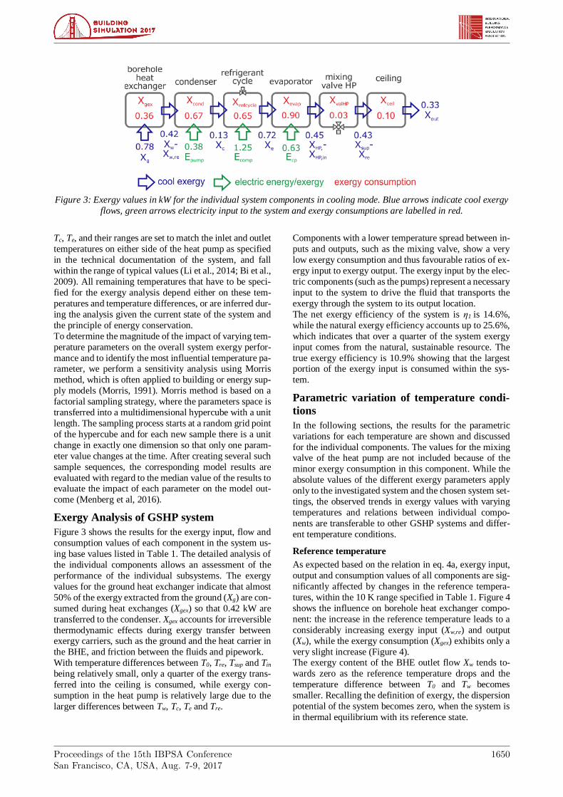
Figure 3: Exergy values in kW for the individual system components in cooling mode. Blue arrows indicate cool exergy

flows, green arrows electricity input to the system and exergy consumptions are labelled in red.

Tc, Te, and their ranges are set to match the inlet and outlet

temperatures on either side of the heat pump as specified

in the technical documentation of the system, and fall

within the range of typical values (Li et al., 2014; Bi et al.,

2009). All remaining temperatures that have to be speci-

fied for the exergy analysis depend either on these tem-

peratures and temperature differences, or are inferred dur-

ing the analysis given the current state of the system and

the principle of energy conservation.

To determine the magnitude of the impact of varying tem-

perature parameters on the overall system exergy perfor-

mance and to identify the most influential temperature pa-rameter, we perform a sensitivity analysis using Morris

method, which is often applied to building or energy sup-

ply models (Morris, 1991). Morris method is based on a

factorial sampling strategy, where the parameters space is

transferred into a multidimensional hypercube with a unit

length. The sampling process starts at a random grid point

of the hypercube and for each new sample there is a unit

change in exactly one dimension so that only one param-

eter value changes at the time. After creating several such

sample sequences, the corresponding model results are

evaluated with regard to the median value of the results to evaluate the impact of each parameter on the model out-

come (Menberg et al, 2016).

Exergy Analysis of GSHP system

Figure 3 shows the results for the exergy input, flow and

consumption values of each component in the system us-

ing base values listed in Table 1. The detailed analysis of

the individual components allows an assessment of the

performance of the individual subsystems. The exergy

values for the ground heat exchanger indicate that almost

50% of the exergy extracted from the ground (Xg) are con-

sumed during heat exchanges (Xgex) so that 0.42 kW are

transferred to the condenser. Xgex accounts for irreversible

thermodynamic effects during exergy transfer between exergy carriers, such as the ground and the heat carrier in

the BHE, and friction between the fluids and pipework.

With temperature differences between T0, Tre, Tsup and Tin

being relatively small, only a quarter of the exergy trans-

ferred into the ceiling is consumed, while exergy con-

sumption in the heat pump is relatively large due to the

larger differences between Tw, Tc, Te and Tre.

Components with a lower temperature spread between in-

puts and outputs, such as the mixing valve, show a very

low exergy consumption and thus favourable ratios of ex-

ergy input to exergy output. The exergy input by the elec-

tric components (such as the pumps) represent a necessary

input to the system to drive the fluid that transports the

exergy through the system to its output location.

The net exergy efficiency of the system is η1 is 14.6%,

while the natural exergy efficiency accounts up to 25.6%,

which indicates that over a quarter of the system exergy

input comes from the natural, sustainable resource. The

true exergy efficiency is 10.9% showing that the largest portion of the exergy input is consumed within the sys-

tem.

Parametric variation of temperature condi-

tions

In the following sections, the results for the parametric

variations for each temperature are shown and discussed

for the individual components. The values for the mixing valve of the heat pump are not included because of the

minor exergy consumption in this component. While the

absolute values of the different exergy parameters apply

only to the investigated system and the chosen system set-

tings, the observed trends in exergy values with varying

temperatures and relations between individual compo-

nents are transferable to other GSHP systems and differ-

ent temperature conditions.

Reference temperature

As expected based on the relation in eq. 4a, exergy input,

output and consumption values of all components are sig-

nificantly affected by changes in the reference tempera-

tures, within the 10 K range specified in Table 1. Figure 4

shows the influence on borehole heat exchanger compo-

nent: the increase in the reference temperature leads to a

considerably increasing exergy input (Xw,re) and output

(Xw), while the exergy consumption (Xgex) exhibits only a

very slight increase (Figure 4). The exergy content of the BHE outlet flow Xw tends to-

wards zero as the reference temperature drops and the

temperature difference between T0 and Tw becomes

smaller. Recalling the definition of exergy, the dispersion

potential of the system becomes zero, when the system is

in thermal equilibrium with its reference state.


1651

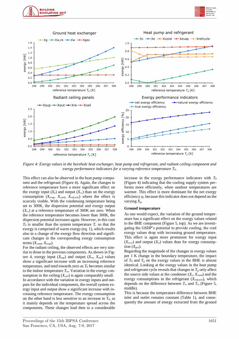
Figure 4: Exergy values in the borehole heat exchanger, heat pump and refrigerant, and radiant ceiling component and

exergy performance indicators for a varying reference temperature T0.

This effect can also be observed in the heat pump compo-

nent and the refrigerant (Figure 4). Again, the changes in

reference temperature have a more significant effect on

the exergy input (Xe) and output (Xc,) than on the exergy

consumption (Xevap, Xcond, Xrefcycle) where the effect is

scarcely visible. With the condensing temperature being

set to 300K, the dispersion potential and exergy output

(Xc,) at a reference temperature of 300K are zero. When

the reference temperature becomes lower than 300K, the

dispersion potential increases again. However, in this case

T0 is smaller than the system temperature Tc so that the exergy is comprised of warm exergy (eq. 1), which results

also in a change of the exergy flow direction and signifi-

cant changes in the corresponding exergy consumption

terms (Xcond, Xevap).

For the radiant ceiling, the observed effects are very sim-

ilar to those in the previous components. As shown in Fig-

ure 4, exergy input (Xsup) and output (Xre, Xout) values

show a significant increase with an increasing reference

temperature, and tend towards zero as T0 becomes similar

to the indoor temperature Tin. Variation in the exergy con-

sumption in the ceiling (Xceil) is again comparably small. In accordance with the variation in exergy inputs and out-

puts for the individual components, the overall system ex-

ergy input and output show a significant increase with in-

creasing reference temperature. The exergy consumption

on the other hand is less sensitive to an increase in T0, as

it mainly depends on the temperature spread across the

components. These changes lead then to a considerable

increase in the exergy performance indicators with T0

(Figure 4) indicating that the cooling supply system per-

forms more efficiently, when outdoor temperatures are

warmer. This effect is more dominant for the net exergy

efficiency η1 because this indicator does not depend on the

varying Xg.

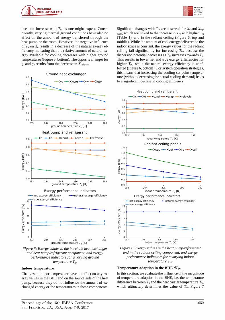
Ground temperature

As one would expect, the variation of the ground temper-

ature has a significant effect on the exergy values related

to the BHE component (Figure 5, top). As we are investi-

gating the GSHP’s potential to provide cooling, the cool

exergy values drop with increasing ground temperature.

This effect is again more prominent for exergy input

(Xw,re) and output (Xw) values than for exergy consump-

tion (Xgex).

Regarding the magnitude of the changes in exergy values

per 1 K change in the boundary temperature, the impact of T0 and Tg on the exergy values in the BHE is almost

identical. Looking at the exergy values in the heat pump

and refrigerant cycle reveals that changes in Tg only affect

the source side values at the condenser (Xc, Xcond) and the

exergy consumptions in the refrigerant (Xrefcycle), which

depends on the difference between Tw and Tre (Figure 5,

middle).

This is because the temperature difference between BHE

inlet and outlet remains constant (Table 1), and conse-

quently the amount of energy extracted from the ground


1652

does not increase with Tg, as one might expect. Conse-

quently, varying thermal ground conditions have also no

effect on the amount of energy transferred through the

heat pump or the room. However, the negative influence

of Tg on Xg results in a decrease of the natural exergy ef-

ficiency indicating that the relative amount of natural ex-

ergy available for cooling decreases with higher ground

temperatures (Figure 5, bottom). The opposite changes for

η1 and η3 results from the decrease in Xrefcycle.

Figure 5: Exergy values in the borehole heat exchanger and heat pump/refrigerant component, and exergy

performance indicators for a varying ground

temperature Tg.

Indoor temperature

Changes in indoor temperature have no effect on any ex-

ergy values in the BHE and on the source side of the heat

pump, because they do not influence the amount of ex-

changed energy or the temperatures in these components.

Significant changes with Tin are observed for Xe and Xref-

cycle, which are linked to the increase in Tre with higher Tin

(Table 1), and in the radiant ceiling (Figure 6, top and

middle). While the amount of cool energy delivered to the

indoor space is constant, the exergy values for the radiant

ceiling fall significantly for increasing Tin, because the

dispersion potential decreases as Tin increases towards T0.

This results in lower net and true exergy efficiencies for

higher Tin, while the natural exergy efficiency is unaf-

fected (Figure 6, bottom). For system operation strategies,

this means that increasing the cooling set point tempera-ture (without decreasing the actual cooling demand) leads

to a significant decline in cooling efficiency.

Figure 6: Exergy values in the heat pump/refrigerant and in the radiant ceiling component, and exergy

performance indicators for a varying indoor

temperature Tin.

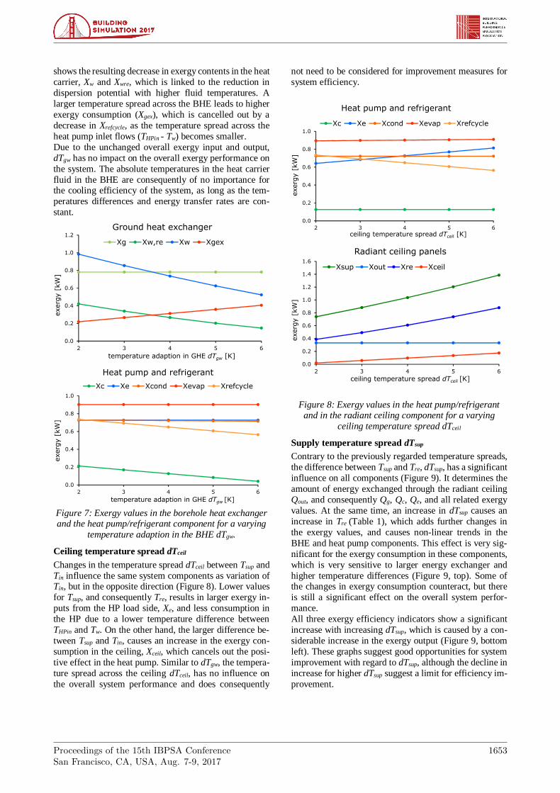
Temperature adaption in the BHE dTgw

In this section, we evaluate the influence of the magnitude of temperature adaption in the BHE, i.e. the temperature

difference between Tg and the heat carrier temperature Tw,

which ultimately determines the value of Tw. Figure 7


1653

shows the resulting decrease in exergy contents in the heat

carrier, Xw and Xwre, which is linked to the reduction in

dispersion potential with higher fluid temperatures. A

larger temperature spread across the BHE leads to higher

exergy consumption (Xgex), which is cancelled out by a

decrease in Xrefcycle, as the temperature spread across the

heat pump inlet flows (THPin - Tw) becomes smaller.

Due to the unchanged overall exergy input and output,

dTgw has no impact on the overall exergy performance on

the system. The absolute temperatures in the heat carrier

fluid in the BHE are consequently of no importance for the cooling efficiency of the system, as long as the tem-

peratures differences and energy transfer rates are con-

stant.

Figure 7: Exergy values in the borehole heat exchanger and the heat pump/refrigerant component for a varying

temperature adaption in the BHE dTgw.

Ceiling temperature spread dTceil

Changes in the temperature spread dTceil between Tsup and

Tin influence the same system components as variation of Tin, but in the opposite direction (Figure 8). Lower values

for Tsup, and consequently Tre, results in larger exergy in-

puts from the HP load side, Xe, and less consumption in

the HP due to a lower temperature difference between

THPin and Tw. On the other hand, the larger difference be-

tween Tsup and Tin, causes an increase in the exergy con-

sumption in the ceiling, Xceil, which cancels out the posi-

tive effect in the heat pump. Similar to dTgw, the tempera-

ture spread across the ceiling dTceil, has no influence on

the overall system performance and does consequently

not need to be considered for improvement measures for

system efficiency.

Figure 8: Exergy values in the heat pump/refrigerant and in the radiant ceiling component for a varying

ceiling temperature spread dTceil

Supply temperature spread dTsup

Contrary to the previously regarded temperature spreads,

the difference between Tsup and Tre, dTsup, has a significant

influence on all components (Figure 9). It determines the

amount of energy exchanged through the radiant ceiling

Qout, and consequently Qg, Qc, Qe, and all related exergy

values. At the same time, an increase in dTsup causes an

increase in Tre (Table 1), which adds further changes in

the exergy values, and causes non-linear trends in the

BHE and heat pump components. This effect is very sig-

nificant for the exergy consumption in these components,

which is very sensitive to larger energy exchanger and

higher temperature differences (Figure 9, top). Some of the changes in exergy consumption counteract, but there

is still a significant effect on the overall system perfor-

mance.

All three exergy efficiency indicators show a significant

increase with increasing dTsup, which is caused by a con-

siderable increase in the exergy output (Figure 9, bottom

left). These graphs suggest good opportunities for system

improvement with regard to dTsup, although the decline in

increase for higher dTsup suggest a limit for efficiency im-

provement.


1654

Figure 9: Exergy values in the borehole heat exchanger, heat pump/refrigerant, and radiant ceiling component and

exergy performance indicators for a varying supply temperature spread dTsup.

Sensitivity analysis with Morris method

The results from the sensitivity analysis with Morris

method are displayed in Table 2 and show the overall magnitude of influence of the selected boundary temper-

atures and temperature spreads on the three investigated

exergy efficiency indicators. For the interpretation of

Morris method results, it is important to distinguish be-

tween negligible parameters that have only a very small,

but noticeable, impact on the model outcome and param-

eters that exhibit exact zero values and have absolutely no

effect on the model results.

The values in Table 2 reveal that of the three examined

temperature boundaries, the reference temperature T0 has

the largest impact on all three performance indicators. Tg

has a significant impact on the natural exergy efficiency,

but only a minor impact on the net and true exergy effi-

ciency, which can be explained by the rather large amount of exergy input through the electric equipment compared

to the amount of exergy from the ground. The indoor tem-

perature has no effect on the natural exergy efficiency, as

observed for variation of Tin above, and significantly less

impact on the other two indicators than T0.

Regarding the impact of the investigated temperature

spreads across different system parts, the supply temper-

ature spread dTsup has clearly the most significant impact,

which is in the same order of magnitude as the effect of

T0. dTgw and dTceil only influence those performance indi-

cators that relate to the components they affect (see dis-

cussion above), and only to a negligible amount, because their effects often cancel out through other components.

Table 2: Results for sensitivity analysis with Morris method as median values of the elementary effects in kW for the

investigated temperature parameters and exergy performance indicators.

Performance indicators T0 Tg Tin dTgw dTceil dTsup

Net exergy efficiency 11.39 1.36 6.43 0 9 × 10-15 8.60

Natural exergy efficiency 7.01 4.39 0 5 ×10-15 0 12.27

True exergy efficiency 8.42 1.53 4.97 0 5 ×10-15 5.71


1655

Conclusion

Examination of a detailed thermodynamic model of a

GSHP cooling system with the concept of warm and cool

exergy enables an in-depth assessment of the utility of in-

dividual system components, such as the borehole heat

exchanger (BHE), the heat pump, and the radiant ceiling.

This study reveals that the exergy consumption in these

components is closely related to the temperature spread

across the individual subsystems. For example, subsys-

tems with a smaller temperature difference between

source and load side, such as the BHE and radiant ceiling,

have lower exergy consumption than the components of the heat pump.

Parametric variation of fluid temperatures, by varying pa-

rameters such as the adaption of the heat carrier fluid in

the BHE dTgw, results in significant changes in exergy val-

ues within the individual components and reveals diverse

interactions between components. In particular, the differ-

ences in exergy consumption terms resulting from tem-

perature changes often counteract each other so that the

overall system performance remains constant over the in-

vestigated temperature ranges. As shown in Figures 7 and

8, this effect is primarily observed for changes in absolute fluid temperatures that only influence the exergy values

in certain components, where the changes in exergy con-

sumption then cancel out.

Changes in system temperatures, such as the ground tem-

perature Tg, on the other hand are found to influence the

overall system performance, as they cause changes in the

amount of energy exchanged between components, or al-

ter the temperature spread across the entire system, i.e.

from the ground to the indoor space (see Figure 9). Hence,

the boundary temperatures of the cooling system, Tg and

Tin, play an important role for the system efficiency and

should be considered carefully for system design, evalua-tion and operation.

The reference temperature, T0, has the by far largest im-

pact on the system efficiency, which is not surprising

given its dominant role in the governing equations. Thus,

the type and value of the temperature used as reference

condition should be carefully considered. The tempera-

ture difference dTsup, which determines the energy output,

is found to be almost as influential as T0, and consequently

offers opportunities for potential system improvement.

In addition, we find that varying temperatures, such as the

reference or ground temperature, across wide ranges re-quire special attention to the temperature relations within

the subsystems, as they determine the type of exergy

(warm or cool) and the flow direction of exergy. These

results demonstrate how exergy analysis, in contrast to en-

ergy analysis, enables a better assessment of the utility

within each individual component of an energy system.

As such, it offers a powerful framework through which

one can identify critical parameters influencing system

(in)efficiencies across its components. Thus, incorporat-

ing exergy models into existing energy simulation tools

appears to be a promising option to further enhance in-

depth system performance analysis. However, further work is needed to adapt our steady-state model in order to

enable coupling to transient system or building simula-

tions.

Acknowledgements

This study is supported by EPSRC grant (EP/L024452/1):

Bayesian Building Energy Management (B-bem).

References

Kazanci, O.B., Shukuya, M. and B.W. Olesen (2016).

Theoretical analysis of the performance of different

cooling strategier with the concept of cool exergy.

Building and Environment 100, 102-113.

Menberg, K., Heo, Y. and R. Choudhary (2016).

Sensitivity analysis methods for building energy

models: Comparing computational costs and

extractable information, Energy and Buildings 133,

433-445.

Morris, M. D. (1991). Factorial sampling plans for

preliminary computational experiments.

Technometrics 33, 161-174.

Li, R., Ooka, R. and M. Shukuya (2014). Theoretical

analysis on ground source heat pump and air source

heat pump systems by the concepts of cool and warm

exergy, Energy and Buildings 75, 447-455.

Schmidt, D. (2009). Low exergy systems for high-

performance buildings and communities, Energy

and Buildings 41, 331-336.

Shukuya, M. (2013). Exergy: theory and applications in

the built environment. Springer, 364 p.

Bi, Y., Wang, X., Liu, Y., Zhang, H. and L. Chen (2009).

Comprehensive exergy analysis of a ground-source

heat pump system for both building heating and

cooling modes. Applied Energy 86, 2560-2565.

Zhou, Y. and G. Gong (2013). Exergy analysis of the building heating and cooling system from the power

plant to the building envelop with hourly variable

reference state. Energy and Buildings 56, 94-99.

Documents

Exergy Analysis of a Ground-Source Heat Pump … Analysis of a Ground-Source Heat Pump System Kathrin Menberg1,2, Yeonsook Heo2, Wonjun Choi 3, Ryozo Ooka , Ruchi Choudhary1, Masanori