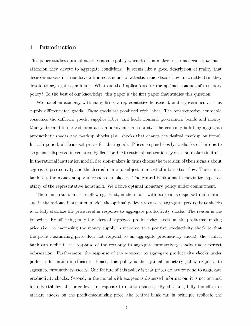
Exogenous Information, Endogenous Information and

Optimal Monetary Policy∗

Luigi Paciello

Einaudi Institute for Economics and Finance

Mirko Wiederholt

Northwestern University

November 2010

Abstract

Most of the analysis of optimal monetary policy is conducted with the Calvo model. This

paper studies optimal monetary policy when the slow adjustment of the price level is due to

imperfect information by decision-makers in firms. We consider two models: a model with ex-

ogenous dispersed information and a rational inattention model. In the model with exogenous

dispersed information, complete stabilization of the price level is optimal after aggregate pro-

ductivity shocks but not after markup shocks. By contrast, in the rational inattention model,

complete stabilization of the price level is optimal both after aggregate productivity shocks and

after markup shocks. Moreover, in the model with exogenous dispersed information, there is no

value from commitment to a future monetary policy. By contrast, in the rational inattention

model, there is value from commitment to a future monetary policy because then the private

sector can trust the central bank that not paying attention to certain variables is optimal.

JEL: E3, E5, D8.

Keywords: dispersed information, rational inattention, optimal monetary policy

∗We thank Fernando Alvarez, Andy Atkeson, Larry Christiano, Jordi Gali, Christian Hellwig, Jonathan Parker,

Alessandro Pavan, Aleh Tsyvinski, Pierre-Olivier Weill and seminar participants at CREI, EIEF, IAE, Maryland,

NBER Summer Institute 2010, Northwestern, SED 2010 and UCLA for helpful comments.

1

1 Introduction

This paper studies optimal macroeconomic policy when decision-makers in firms decide how much

attention they devote to aggregate conditions. It seems like a good description of reality that

decision-makers in firms have a limited amount of attention and decide how much attention they

devote to aggregate conditions. What are the implications for the optimal conduct of monetary

policy? To the best of our knowledge, this paper is the first paper that studies this question.

We model an economy with many firms, a representative household, and a government. Firms

supply differentiated goods. These goods are produced with labor. The representative household

consumes the different goods, supplies labor, and holds nominal government bonds and money.

Money demand is derived from a cash-in-advance constraint. The economy is hit by aggregate

productivity shocks and markup shocks (i.e., shocks that change the desired markup by firms).

In each period, all firms set prices for their goods. Prices respond slowly to shocks either due to

exogenous dispersed information by firms or due to rational inattention by decision-makers in firms.

In the rational inattention model, decision-makers in firms choose the precision of their signals about

aggregate productivity and the desired markup, subject to a cost of information flow. The central

bank sets the money supply in response to shocks. The central bank aims to maximize expected

utility of the representative household. We derive optimal monetary policy under commitment.

The main results are the following. First, in the model with exogenous dispersed information

and in the rational inattention model, the optimal policy response to aggregate productivity shocks

is to fully stabilize the price level in response to aggregate productivity shocks. The reason is the

following. By offsetting fully the effect of aggregate productivity shocks on the profit-maximizing

price (i.e., by increasing the money supply in response to a positive productivity shock so that

the profit-maximizing price does not respond to an aggregate productivity shock), the central

bank can replicate the response of the economy to aggregate productivity shocks under perfect

information. Furthermore, the response of the economy to aggregate productivity shocks under

perfect information is efficient. Hence, this policy is the optimal monetary policy response to

aggregate productivity shocks. One feature of this policy is that prices do not respond to aggregate

productivity shocks. Second, in the model with exogenous dispersed information, it is not optimal

to fully stabilize the price level in response to markup shocks. By offsetting fully the effect of

markup shocks on the profit-maximizing price, the central bank can in principle replicate the

2

response of the economy to markup shocks under perfect information. However, the response of

the economy to markup shocks under perfect information is inefficient. In particular, there is

inefficient consumption variance. By offsetting only partially the effect of markup shocks on the

profit-maximizing price, the central bank increases inefficient price dispersion but reduces inefficient

consumption variance (relative to the perfect-information solution). Accepting some inefficient price

dispersion in exchange for reduced consumption variance turns out to be the optimal monetary

policy. At the optimal monetary policy, the profit-maximizing price, actual prices, and the price

level respond to markup shocks. By contrast, in the rational inattention model, it is optimal to fully

stabilize the price level in response to markup shocks. By counteracting the effect of markup shocks

on the profit-maximizing price (i.e., by reducing the money supply in response to a positive markup

shock), the central bank reduces the variance of the profit-maximizing price due to markup shocks,

which now reduces both inefficient price dispersion and the attention that decision-makers in firms

devote to markup shocks. The latter reduces the response of the price level to markup shocks and

thereby reduces consumption variance due to markup shocks. Hence, the trade-off between price

dispersion and consumption variance due to markup shocks disappears. Reducing the money supply

more in response to a positive markup shock now reduces both price dispersion and consumption

variance. The optimal monetary policy is to counteract the effect of markup shocks on the profit-

maximizing price until the variance of the profit-maximizing price due to the markup shock is

sufficiently small so that decision-makers in firms pay no attention to markup shocks. Thus, at the

optimal monetary policy, prices do not respond to markup shocks. In summary, in the rational

inattention model, the trade-off between price dispersion and consumption variance due to markup

shocks disappears and therefore complete price level stability is optimal. This is important because

the trade-off between price dispersion and consumption variance due to markup shocks has been

emphasized a lot in the literature on optimal monetary policy in the New Keynesian model. Third,

in the model with exogenous dispersed information, there is no value from commitment to a future

monetary policy. By contrast, in the rational inattention model, there is value from commitment

to a future monetary policy because then the private sector can trust the central bank that not

paying attention to certain variables is optimal.

This paper is related to four papers that also study optimal monetary policy in models in which

price setting firms have imperfect information. First, Ball, Mankiw and Reis (2005) study optimal

3

monetary policy in the sticky information model of Mankiw and Reis (2002). The main difference

between their paper and our paper is that in their paper the information structure is exogenous.

In particular, in their paper the probability with which firms update their information sets is

independent of monetary policy. Second, Adam (2007) studies optimal monetary policy in a model

in which firms pay limited attention to aggregate variables. In his model the amount of attention

that firms devote to aggregate variables is exogenous; whereas in the rational inattention model

presented below the amount of attention that firms devote to aggregate variables is endogenous (and

depends on monetary policy). We show that this changes optimal monetary policy in a fundamental

way. Third, Lorenzoni (2010) and Angeletos and La’O (2008) study optimal monetary policy in

models with dispersed information. In Lorenzoni (2010), price setting firms observe the history of

the economy up to the previous period, the sum of aggregate and idiosyncratic productivity, and a

noisy public signal about aggregate productivity. There are several differences between his paper

and our paper: (i) in his paper the “noise” in the private signal concerning aggregate productivity is

idiosyncratic productivity, while in our paper the noise arises from limited attention, (ii) in his paper

the information structure is exogenous, while in our paper the information structure is endogenous,

and (iii) in his paper the central bank has imperfect information, while we assume that the central

bank has perfect information about the state of the economy. We make this assumption to derive

the optimal monetary policy response to changes in fundamentals. Afterwards, we study whether

the central bank can also implement this optimal monetary policy response with less information.

Like in Lorenzoni (2010), agents in Angeletos and La’O (2008) observe the history of the economy

up to the previous period, the sum of aggregate and idiosyncratic productivity, and a noisy public

signal about aggregate productivity. In addition, in Angeletos and La’O (2008) agents observe

noisy signals concerning endogenous variables with exogenous variance of noise. This creates an

informational externality because a stronger response of agents to their private signals makes the

signals concerning endogenous variables more informative. Angeletos and La’O (2008) study how

this informational externality affects optimal fiscal and monetary policy. In summary, this paper is

the first paper that studies optimal monetary policy in a model in which agents choose the attention

that they allocate to aggregate variables.

This paper is also related to the literature on the social value of public information, for example,

Morris and Shin (2002), Hellwig (2005), and Angeletos and Pavan (2007). In this literature, the

4

main monetary policy question is whether the central bank should provide information about

economic fundamentals. We instead ask how the central bank should set the money supply or a

nominal interest rate in response to fundamentals. In addition, in the literature on the social value

of public information the information structure (i.e., what agents observe) is typically exogenous.

The rest of the paper is organized as follows. Section 2 presents the model setup. Section 3

specifies the objective of the central bank. Section 4 states the optimal monetary policy problem

under commitment in the model with an exogenous information structure and in the model with an

endogenous information structure. Section 5 shows that there is a monetary policy that replicates

the allocation under perfect information. Section 6 derives the optimal monetary policy response to

aggregate productivity shocks. Section 7 derives the optimal monetary policy response to markup

shocks. Section 8 contains additional results. Section 9 concludes.

2 Model setup

The economy is populated by a representative household, firms, and a government.

Household: The household’s preferences in period zero over sequences of consumption and

labor supply {Ct, Lt}∞t=0 are given by

E0

" ∞Xt=0

βt

ÃC1−γt − 11− γ

− L1+ψt

1 + ψ

!#, (1)

where Ct is composite consumption and Lt is labor supply in period t. Here E0 denotes the

expectation operator conditioned on information of the household in period zero. The parameter

β ∈ (0, 1) is the discount factor. The parameter γ > 0 is the inverse of the intertemporal elasticity

of substitution and the parameter ψ ≥ 0 is the inverse of the Frisch elasticity of labor supply.

Composite consumption in period t is given by a Dixit-Stiglitz aggregator

Ct =

Ã1

I

IXi=1

C1

1+Λti,t

!1+Λt, (2)

where Ci,t is consumption of good i in period t. There are I different consumption goods and the

elasticity of substitution between those different consumption goods equals (1 + 1/Λt) in period t.

The variable Λt will equal the desired markup by firms in period t. Therefore, we call Λt the desired

markup. We assume that the log of the desired markup follows a stationary Gaussian first-order

5

autoregressive process

ln (Λt) = (1− ρλ) ln (Λ) + ρλ ln (Λt−1) + νt, (3)

where the parameter Λ > 0, the parameter ρλ ∈ [0, 1), and the innovation νt is i.i.d.N¡0, σ2ν

¢. We

call the innovation νt a markup shock. We introduce the markup shock in the model as an example

of a shock that has the following property: the response of the economy to the shock under perfect

information is inefficient.1 We call this property of a shock the inefficiency property. In Section 6

we derive the optimal monetary policy response to a markup shock. In Section 8 we show that our

results concerning the optimal monetary policy response to a markup shock extend to other shocks

that have the inefficiency property.

The flow budget constraint of the representative household in period t reads

Mt +Bt = Rt−1Bt−1 +WtLt +Dt − Tt +

ÃMt−1 −

IXi=1

Pi,t−1Ci,t−1

!. (4)

The right-hand side of the flow budget constraint is pre-consumption wealth in period t. Here Bt−1

are the household’s holdings of nominal government bonds between periods t − 1 and t, Rt−1 is

the nominal gross interest rate on those bond holdings, Wt is the nominal wage rate in period t,

Dt are nominal aggregate profits in period t, Tt are nominal lump sum taxes in period t, and the

term in brackets are unspent nominal money balances carried over from period t − 1 to period t.

The representative household can transform his pre-consumption wealth in period t into money

balances, Mt, and bond holdings, Bt. The purpose of holding money is to purchase goods. We

assume that the representative household faces the following cash-in-advance constraint

IXi=1

Pi,tCi,t =Mt. (5)

The representative household also faces a no-Ponzi-scheme condition.

We introduce the cash-in-advance constraint because it allows us to explain the intuition behind

our results concerning optimal monetary policy in a very simple way. In Section 8 we show that our

results concerning optimal monetary policy extend to a cashless economy à la Woodford (2003).

Furthermore, recall that there are different formulations of the cash-in-advance constraint and note

that in the formulation of the cash-in-advance constraint that we use there are no monetary frictions

because wage income can be immediately transformed into cash and cash can be immediately spent1We define efficiency formally in Section 3.

6

on goods. We decided to abstract from monetary frictions in our benchmark economy for two

reasons: (i) abstracting from monetary frictions is common in the New Keynesian literature on

optimal monetary policy and therefore abstracting from monetary frictions facilitates comparison

of optimal monetary policy in the two models that we consider to optimal monetary policy in the

standard New Keynesian model, and (ii) we think it is useful to study in isolation the implications

of different frictions for optimal monetary policy. In Section 8 we consider an extension with

monetary frictions and there we study how monetary frictions affect optimal monetary policy in

the two models that we consider.

In every period, the representative household chooses a consumption vector, labor supply, nom-

inal money balances, and nominal bond holdings. The representative household takes as given the

nominal interest rate, the nominal wage rate, nominal aggregate profits, nominal lump sum taxes,

and the prices of all consumption goods.

Firms: There are I firms. Firm i supplies good i. The technology of firm i is given by

Yi,t = AtLαi,t, (6)

where Yi,t is output and Li,t is labor input of firm i in period t. At is aggregate productivity in

period t. The parameter α ∈ (0, 1] is the elasticity of output with respect to labor input. The log

of aggregate productivity follows a stationary Gaussian first-order autoregressive process

ln (At) = ρa ln (At−1) + εt, (7)

where the parameter ρa ∈ [0, 1) and the innovation εt is i.i.d.N¡0, σ2ε

¢. The processes {At} and

{Λt} are assumed to be independent. We call the innovation εt an aggregate productivity shock.

We introduce the aggregate productivity shock in the model as an example of a shock that has

the following property: the response of the economy to the shock under perfect information is

efficient. We call this property of a shock the efficiency property. In Section 6 we derive the

optimal monetary policy response to an aggregate productivity shock. In Section 8 we show that

the results concerning the optimal monetary policy response to an aggregate productivity shock

extend to other shocks that have the efficiency property.

Nominal profits of firm i in period t equal

(1 + τp)Pi,tYi,t −WtLi,t, (8)

7

where τp is a production subsidy paid by the government.

In every period, each firm sets a price and commits to supply any quantity at that price. Each

firm takes as given composite consumption by the representative household, the nominal wage rate,

and the following price index2

Pt =

Ã1

I

IXi=1

P− 1

Λti,t

!−ΛtI. (9)

Government: There is a monetary authority and a fiscal authority. The monetary authority

commits to set the money supply according to the following rule

ln (Mst ) = Ft (L) εt +Gt (L) νt, (10)

whereMst denotes the money supply in period t. Ft (L) andGt (L) are infinite-order lag polynomials

which can depend on t. The last equation simply says that the log of the money supply in period t

can be any linear function of the sequence of shocks up to and including period t. We will ask the

question which linear function is optimal.

Two remarks may be useful. First, the reader may wonder how the money market clears at a

given money supply. In equilibrium, the endogenous variables (e.g., the price level, the nominal

interest rate, and consumption) adjust such that the demand for money balances by the represen-

tative household equals the supply of money balances by the monetary authority (i.e., Mt =Mst ).

Second, in equation (10) we assume that the central bank can commit to a money supply rule.

In Section 8 we show that the set of attainable allocations is identical when the central bank can

commit to an interest rate rule of the form

ln (Rt) = Ft (L) εt +Gt (L) νt. (11)

The drawback of an interest rate rule is that multiplicity of equilibria at a given monetary policy

arises more easily. Therefore, we assume in the benchmark economy that the central bank can

commit to a money supply rule and we postpone the discussion of unique implementation in the

case of an interest rate rule to Section 8.2Dixit and Stiglitz (1977), in their seminal article on monopolistic competition, also assume that there is a finite

number of physical goods and that firms take the price index as given. Moreover, it seems to be a good description

of the U.S. economy that there is a finite number of physical consumption goods and that firms take the consumer

price index as given.

8

Next, consider fiscal policy. The government budget constraint in period t reads

Tt +Bt = Rt−1Bt−1 + τp

ÃIX

i=1

Pi,tYi,t

!. (12)

The government has to finance maturing nominal government bonds and the production subsidy.

The government can collect lump sum taxes or issue new one-period nominal government bonds.

We assume that the fiscal authority pursues a Ricardian fiscal policy. For ease of exposition, we

assume that the fiscal authority fixes nominal government bonds at some non-negative level

Bt = B ≥ 0. (13)

Furthermore, we assume that the fiscal authority sets the production subsidy so as to correct, in

the non-stochastic steady state, the distortion arising from monopolistic competition. Formally,

τp = Λ. (14)

Alternatively, one could assume that the fiscal authority sets the production subsidy so as to correct

perfectly at each point in time the distortion arising from monopolistic competition. Formally,

τp,t = Λt. (15)

However, since in the United States fiscal policy has to be approved by Congress while monetary

policy decisions are implemented directly by the Federal Reserve, we find it more realistic to assume

that the fiscal authority cannot adjust the production subsidy quickly while the monetary authority

can adjust the money supply quickly.

Information: We consider two models, one with an exogenous information structure and one

with an endogenous information structure. In both models, the information set in period t of the

decision-maker who is responsible for setting the price of good i is

Ii,t = Ii,−1 ∪ {si,0, si,1, . . . , si,t} , (16)

where Ii,−1 contains any initial information that the price setter of firm i has in period minus one

and si,t is the signal that the price setter of firm i receives in period t. We assume that the structure

of the economy is common knowledge in period minus one. Furthermore, in the model with an

exogenous information structure, we assume that the price setter of firm i receives in every period

9

t ≥ 0 a two-dimensional signal consisting of a noisy signal concerning aggregate productivity and

a noisy signal concerning the desired markup:

si,t =

⎛⎝ ln (At) + ηi,t

ln (Λt/Λ) + ζi,t

⎞⎠ , (17)

where the noise terms have the following properties: (i) the stochastic processes©ηi,tªand

©ζi,tª

are independent of the stochastic processes {At} and {Λt}, (ii) the stochastic processes©ηi,tªand©

ζi,tªare independent across firms and independent of each other, and (iii) the noise term ηi,t is

i.i.d.N¡0, σ2η

¢and the noise term ζi,t is i.i.d.N

³0, σ2ζ

´. In the model with an exogenous information

structure, the variances of noise σ2η and σ2ζ are structural parameters.

By contrast, in the model with an endogenous information structure, the variances of noise

σ2η and σ2ζ are endogenous. Following the literature on rational inattention, we assume that the

decision-maker who is responsible for setting the price of good i chooses the variances of noise

subject to an information flow constraint. Formally, the price setter of firm i solves the following

decision problem in period minus one:

max(1/σ2η,1/σ2ζ)∈R2+

(Ei,−1

" ∞Xt=0

βtπ (Pi,t, Pt, Ct,Wt, At,Λt)

#− μ

1− βκ

), (18)

subject to equations (16)-(17) and in every period t ≥ 0

Pi,t = arg maxx∈R++

Ei,t[π (x,Pt, Ct,Wt, At,Λt)], (19)

and

1

2log2

⎛⎝σ2a|st−1i

σ2a|sti

⎞⎠+ 12log2

⎛⎝σ2λ|st−1i

σ2λ|sti

⎞⎠ = κ. (20)

Here Ei,t denotes the expectation operator conditioned on the information of the price setter of

firm i in period t, π denotes the real profit function defined as the nominal profit function times

the marginal utility of consumption of the representative household divided by Pt, σ2a|stidenotes the

conditional variance of at ≡ ln (At) given information of the price setter of firm i in period t, and

σ2λ|sti

denotes the conditional variance of λt ≡ ln (Λt/Λ) given information of the price setter of firm

i in period t. The variable κ is the per-period information flow concerning aggregate conditions and

the parameter μ > 0 is the per-period marginal cost of information flow. The decision-maker chooses

the precision of the two signals in period minus one so as to maximize the expected discounted sum

10

of profits net of the cost of information flow. The decision-maker takes into account how his/her

choice of signal precision affects future price setting behavior. Furthermore, equation (20) measures

the information flow concerning aggregate conditions and objective (18) states that information flow

concerning aggregate conditions is costly. We interpret the cost μ as the price setter’s opportunity

cost of devoting attention to aggregate conditions.

Three remarks are in place before we proceed. First, we interpret the noise in the signal (17)

as arising from the limited attention of the price setter of firm i. Therefore, we find it reasonable

to assume that the noise is idiosyncratic. Second, in equation (17) we assume that the price setter

of firm i receives independent signals concerning aggregate productivity and the desired markup.

In Section 8 we show that this assumption has no effect on optimal monetary policy in the model

with an endogenous information structure. We show that optimal monetary policy in the model

with an endogenous information structure is exactly the same when the decision-maker can choose

to receive signals concerning any linear combination of at and λt. Third, in the decision problem

given in the previous paragraph the price setter of firm i chooses signal precision once and for all.

In Section 8 we show that our propositions concerning optimal monetary policy in the model with

an endogenous information structure also hold when the decision-maker chooses signal precision

period by period.

We assume that the monetary authority has perfect information (i.e., in every period t ≥ 0,

the monetary authority knows the entire history of the economy up to and including period t).

We make this assumption because we are interested in the optimal conduct of monetary policy.

We think this is an interesting benchmark. In Section 8 we also consider an extension where the

monetary authority only knows the price level and composite consumption. In addition, we assume

that the representative household has perfect information. We make this assumption (i) to isolate

the implications of information frictions on the side of price setters for optimal monetary policy,

and (ii) to facilitate the comparison to optimal monetary policy in the simplest New Keynesian

model, where the only friction apart from monopolistic competition is price stickiness.

Aggregation: When we compute the price index terms will appear that are linear in 1I

XI

i=1ηi,t

and 1I

XI

i=1ζi,t. These averages are random variables with mean zero and variance 1

Iσ2η and

1Iσ

2ζ ,

respectively. We will neglect these terms because these terms have mean zero and a variance that

can be made arbitrarily small by choosing a sufficiently high number of firms I. For example, one

11

could set I = 10100. We work with a finite number of firms rather than a continuum of firms

because we find that it makes the derivation of the central bank’s objective in the next section

more transparent.

3 Objective of the central bank

We assume that the central bank’s aim is to maximize expected utility of the representative house-

hold, given by equations (1)-(2).

We now derive a simple expression for expected utility by using the fact that one can express

period utility at a feasible allocation as a function only of the consumption vector at time t,

aggregate productivity at time t, and the desired markup at time t. First, at any feasible allocation

the representative household has to supply the labor that is needed to produce the consumption

vector

Lt =IX

i=1

µCi,t

At

¶ 1α

. (21)

Furthermore, equation (2) for the consumption aggregator can be written as

1 =1

I

IXi=1

C1

1+Λti,t ,

where Ci,t ≡ (Ci,t/Ct) denotes relative consumption of good i in period t. Rearranging yields

CI,t =

ÃI −

I−1Xi=1

C1

1+Λti,t

!1+Λt. (22)

Substituting equations (21) and (22) into the period utility function in (1) yields the following

expression for period utility at a feasible allocation

U³Ct, C1,t, . . . , CI−1,t, At,Λt

´=

C1−γt − 11− γ

− 1

1 + ψ

µCt

At

¶ 1α(1+ψ)

⎡⎣I−1Xi=1

C1αi,t +

ÃI −

I−1Xi=1

C1

1+Λti,t

! 1α(1+Λt)

⎤⎦1+ψ .(23)

Hence, expected utility at a feasible allocation equals

E

" ∞Xt=0

βtU³Ct, C1,t, . . . , CI−1,t, At,Λt

´#. (24)

12

In summary, by substituting the technology and the consumption aggregator into the period utility

function one can express period utility at time t as a function only of composite consumption, the

consumption mix, aggregate productivity, and the desired markup at time t.

Next, we study the efficient allocation. The efficient allocation in period t, defined as the feasible

allocation in period t that maximizes utility of the representative household, is

C∗t =³ α

I1+ψ

´ 1

γ−1+ 1α (1+ψ) A

1α (1+ψ)

γ−1+ 1α (1+ψ)

t , (25)

and, for all i = 1, . . . , I − 1,

C∗i,t = 1. (26)

Efficient composite consumption in period t is strictly increasing in aggregate productivity at time

t. The efficient consumption mix in period t is to consume an equal amount of each good. Note

that the efficient consumption vector is independent of the desired markup.

In the following sections, we work with a log-quadratic approximation of expected utility (24)

around the non-stochastic steady state. In the rest of the paper, variables without time subscript

denote values in the non-stochastic steady state and small variables denote log-deviations from the

non-stochastic steady state (e.g., ct = ln (Ct/C) and ci,t = ln³Ci,t/Ci

´). Due to the production

subsidy (14), the non-stochastic steady state is efficient. Expressing the function U given by

equation (23) in terms of log-deviations from the non-stochastic steady state and using C = C∗

and Ci = C∗i yields the following expression for period utility at a feasible allocation

u (ct, c1,t, . . . , cI−1,t, at, λt)

=C1−γe(1−γ)ct − 1

1− γ

−C1−γe

1α(1+ψ)(ct−at)

1α (1 + ψ)

⎡⎣1I

I−1Xi=1

e1αci,t +

1

I

ÃI −

I−1Xi=1

eci,t

1

1+Λeλt

! 1α(1+Λe

λt)⎤⎦1+ψ . (27)

Proposition 1 (Objective of the central bank) Let u denote the second-order Taylor approximation

to the period utility function u at the origin. Let E denote the unconditional expectation operator.

13

Let xt, zt, and ωt denote the following vectors

xt =³ct c1,t · · · cI−1,t

´0, (28)

zt =³at λt

´0, (29)

ωt =³x0t z0t 1

´0. (30)

Let ωn,t denote the nth element of ωt. Suppose that there exist two constants δ < (1/β) and φ ∈ R

such that, for each period t ≥ 0 and for all n and k,

E |ωn,tωk,t| < δtφ. (31)

Then

E

" ∞Xt=0

βtu (xt, zt)

#= E

" ∞Xt=0

βtu (x∗t , zt)

#+

∞Xt=0

βtE

∙1

2(xt − x∗t )

0H (xt − x∗t )

¸, (32)

where the matrix H is given by

H = −C1−γ

⎡⎢⎢⎢⎢⎢⎢⎢⎢⎢⎢⎣

γ − 1 + 1α (1 + ψ) 0 · · · · · · 0

0 2 1+Λ−αI(1+Λ)α1+Λ−αI(1+Λ)α · · · 1+Λ−α

I(1+Λ)α... 1+Λ−α

I(1+Λ)α

. . . . . ....

......

. . . . . . 1+Λ−αI(1+Λ)α

0 1+Λ−αI(1+Λ)α . . . 1+Λ−α

I(1+Λ)α 2 1+Λ−αI(1+Λ)α

⎤⎥⎥⎥⎥⎥⎥⎥⎥⎥⎥⎦, (33)

and the vector x∗t is given by

c∗t =1α (1 + ψ)

γ − 1 + 1α (1 + ψ)

at, (34)

and

c∗i,t = 0. (35)

Proof. See Appendix A.

After the log-quadratic approximation of the period utility function (23), expected utility of

the representative household is given by equation (32). The efficient consumption vector in period

t is given by equations (34)-(35) and the utility loss in the case of a deviation from the efficient

consumption vector in period t is given by the quadratic form in square brackets on the right-hand

side of equation (32). The upper-left element of the matrix H determines the utility loss in the

14

case of inefficient composite consumption, while the lower-right block of the matrix H determines

the utility loss in the case of an inefficient consumption mix. Finally, condition (31) ensures that

in the expression on the left-hand side of equation (32) one can change the order of integration

and summation and the infinite sum converges. In the models that we consider, condition (31) is

always satisfied.

4 The Ramsey problem

In this section, we state the problem of the central bank that aims to commit to the money supply

rule that maximizes expected utility of the representative household.

In the model with an exogenous information structure, the problem of the central bank is

max{Ft(L),Gt(L)}∞t=0

E

" ∞Xt=0

βtU³Ct, C1,t, . . . , CI−1,t, At,Λt

´#, (36)

subject to

PtCt =Mt, (37)

Ci,t =

ÃPi,t1IPt

!− 1+ 1Λt

Ct, (38)

Wt

Pt= Lψ

t Cγt , (39)

Pt =

Ã1

I

IXi=1

P− 1

Λti,t

!−ΛtI, (40)

E

∙∂π (Pi,t, Pt, Ct,Wt, At,Λt)

∂Pi,t|Ii,t

¸= 0, (41)

Ii,t = Ii,−1 ∪ {si,0, si,1, . . . , si,t} , (42)

si,t =

⎛⎝ ln (At) + ηi,t

ln (Λt/Λ) + ζi,t

⎞⎠ , (43)

Lt =IX

i=1

µCi,t

At

¶ 1α

, (44)

ln (At) = ρa ln (At−1) + εt, (45)

ln (Λt/Λ) = ρλ ln (Λt−1/Λ) + νt, (46)

15

and

ln (Mt) = Ft (L) εt +Gt (L) νt. (47)

Equations (37)-(40) are the household’s optimality conditions.3 Equation (41) is the firms’ opti-

mality condition and equations (42)-(43) specify the information set of the price setter of firm i in

period t. Equation (44) is the labor market clearing condition, equations (45)-(46) specify the laws

of motion of the exogenous variables, and equation (47) is the equation for the money supply.4 The

function U defined by equation (23) gives period utility at a feasible allocation, Ft (L) and Gt (L)

are infinite-order lag polynomials which can depend on t, and the innovations εt, νt, ηi,t, and ζi,t

have the properties specified in Section 2. In the model with an exogenous information structure,

the variances of noise σ2η and σ2ζ are structural parameters. They do not depend on monetary

policy.

By contrast, in the model with an endogenous information structure, the variances of noise σ2η

and σ2ζ are given by the solution to the problem (18)-(20) and the central bank understands that

the choice of the money supply rule affects the firms’ choice of signal precision.

Next, in the model with an exogenous information structure, a log-quadratic approximation of

the central bank’s objective (36) around the non-stochastic steady state and a log-linear approx-

imation of the equilibrium conditions (37)-(41) and (44) around the non-stochastic steady state

yields the following linear quadratic Ramsey problem

min{Ft(L),Gt(L)}∞t=0

∞Xt=0

βtE

"(ct − c∗t )

2 + δ1

I

IXi=1

(pi,t − pt)2

#, (48)

subject to

c∗t =φaφc

at, (49)

ct = mt − pt, (50)

pt =1

I

IXi=1

pi,t, (51)

pi,t = E£p∗i,t|Ii,t

¤, (52)

3We do not state the consumption Euler equation because here the consumption Euler equation is only a pricing

equation that determines the equilibrium nominal interest rate.4The requirement that each firm produces the quantity demanded is embedded in the profit function π and the

money market clearing condition Mt =Mst is embedded in equation (47).

16

p∗i,t = pt + φcct − φaat + φλλt, (53)

Ii,t = Ii,−1 ∪ {si,0, si,1, . . . , si,t} , (54)

si,t =

⎛⎝ at + ηi,t

λt + ζi,t

⎞⎠ , (55)

at = ρaat−1 + εt, (56)

λt = ρλλt−1 + νt, (57)

and

mt = Ft (L) εt +Gt (L) νt, (58)

where

φc =ψα + γ + 1−α

α

1 + 1−αα

1+ΛΛ

> 0, (59)

φa =ψα +

1α

1 + 1−αα

1+ΛΛ

> 0, (60)

φλ =Λ1+Λ

1 + 1−αα

1+ΛΛ

> 0, (61)

δ =

1+Λ−α(1+Λ)α

¡1 + 1

Λ

¢2γ − 1 + 1

α (1 + ψ)> 0. (62)

Here c∗t is efficient composite consumption in period t, p∗i,t is the profit-maximizing price of firm i

in period t, φc, φa and φλ are the coefficients in the equation for the profit-maximizing price, and

δ is the relative weight on price dispersion in the central bank’s objective.

In the model with an exogenous information structure, the variances of noise are exogenous. By

contrast, in the model with an endogenous information structure, the variances of noise are given

by the solution to problem (18)-(20) and the central bank understands that the money supply rule

affects firms’ allocation of attention. After a log-quadratic approximation of the profit function π

the attention problem (18)-(20) reads

min(1/σ2η,1/σ2ζ)∈R2+

( ∞Xt=0

βtω

2Ei,−1

h¡pi,t − p∗i,t

¢2i+

μ

1− βκ

), (63)

subject to

pi,t = E£p∗i,t|Ii,t

¤, (64)

17

and

1

2log2

⎛⎝σ2a|st−1i

σ2a|sti

⎞⎠+ 12log2

⎛⎝σ2λ|st−1i

σ2λ|sti

⎞⎠ = κ, (65)

where

ω = C−γWLi

P

1+ΛΛ

α

µ1 +

1− α

α

1 + Λ

Λ

¶. (66)

Here p∗i,t is the profit-maximizing price of firm i in period t given by equation (53), Ii,t is the

information set of the price setter of firm i in period t given by equations (54)-(55), and the

coefficient ω determines the loss in profit in the case of a suboptimal price.

5 Perfect information solution and the central bank’s ability to

replicate it

In this section, we derive the solution of the model under perfect information, and we show that

the central bank can always replicate this solution under imperfect information. This intermediate

result will be useful when we derive the optimal monetary policy response to aggregate productivity

shocks in the next section.

Suppose that decision-makers who set prices have perfect information. Then, each firm charges

the profit-maximizing price, and equations (50)-(53) imply that

ct =φaφc

at −φλφc

λt, (67)

pi,t − pt = 0, (68)

and

pt = mt − ct. (69)

The economy’s response to aggregate productivity shocks under perfect information is efficient,

while the economy’s response to markup shocks under perfect information is inefficient. To see this,

note that price dispersion equals zero under perfect information, and compare equilibrium composite

consumption given by equation (67) to efficient composite consumption given by equation (49). The

reason for the inefficient response to markup shocks is that the efficient allocation is independent

of the desired markup but under perfect information firms’ actual markup varies with the desired

markup. Finally, note that monetary policy has no effect on the equilibrium allocation under perfect

18

information. Monetary policy only affects nominal variables. For example, the central bank can

completely stabilize the price level by setting mt =φaφcat − φλ

φcλt but this has no effect on welfare.

The central bank can replicate the perfect information solution under imperfect information with

a particular monetary policy rule. More precisely, when the central bank sets mt =φaφcat − φλ

φcλt,

then the equilibrium allocation under perfect information is also the unique equilibrium allocation

under imperfect information. The proof is as follows. First, substituting equation (50) into equation

(53) yields the following equation for the profit-maximizing price of firm i in period t

p∗i,t = (1− φc) pt + φc

µmt −

φaφc

at +φλφc

λt

¶. (70)

Second, when mt =φaφcat − φλ

φcλt then equations (51), (52), and (70) imply

pt = (1− φc)1

I

IXi=1

E [pt|Ii,t] . (71)

The unique solution to the last equation is pt = 0. Thus, when mt =φaφcat − φλ

φcλt then pt = 0 is

the unique equilibrium price level. Finally, substituting mt =φaφcat− φλ

φcλt and pt = 0 into equation

(50) yields

ct =φaφc

at −φλφc

λt, (72)

and substituting mt =φaφcat − φλ

φcλt and pt = 0 into equations (52) and (70) yields

pi,t = 0, (73)

implying

pi,t − pt = 0. (74)

Hence, when the central bank sets mt =φaφcat− φλ

φcλt, then the equilibrium allocation under perfect

information is also the unique equilibrium allocation under imperfect information. Moreover, the

same arguments also apply shock by shock. By setting Ft (L) εt =φaφcat the central bank can

replicate the response of the economy to aggregate productivity shocks under perfect information.

By setting Gt (L) νt = −φλφcλt the central bank can replicate the response of the economy to markup

shocks under perfect information.

We have derived the solution of the model under perfect information, and we have shown that

the central bank can replicate this solution under imperfect information with a particular monetary

19

policy rule. Hence, if the central bank conducts optimal monetary policy, welfare under imperfect

information has to be weakly larger than welfare under perfect information.

6 Optimal monetary policy response to aggregate productivity

shocks

In this section, we derive the optimal monetary policy response to aggregate productivity shocks.

We begin with the model with an exogenous information structure and we then consider the model

with an endogenous information structure. Equipped with the results of the previous section, the

proofs are straightforward.

Proposition 2 (Exogenous information structure) Consider the Ramsey problem (48)-(62), where

the variances of noise σ2η and σ2ζ are structural parameters. If σ

2η > 0, the unique optimal monetary

policy response to aggregate productivity shocks is

Ft (L) εt =φaφc

at. (75)

At this policy, the unique equilibrium response of the economy to aggregate productivity shocks

equals the efficient response to aggregate productivity shocks, and the price level does not respond

to aggregate productivity shocks.

Proof. First, when Ft (L) εt =φaφcat, the unique equilibrium response of composite consumption

to aggregate productivity shocks equals the perfect information response of composite consumption

to aggregate productivity shocks, and the perfect information response of composite consumption to

aggregate productivity shocks is efficient. See the previous section. Second, when Ft (L) εt =φaφcat,

there is no price dispersion caused by the noise in the signal concerning aggregate productivity.

See again the previous section. Third, if σ2η > 0, any monetary policy rule with Ft (L) εt 6= φaφcat

yields an inefficient response of composite consumption to aggregate productivity shocks or price

dispersion caused by the noise in the signal concerning aggregate productivity: if price setters put

weight on the signal concerning aggregate productivity then there is price dispersion caused by

the noise in the signal concerning aggregate productivity, and if price setters put no weight on the

signal concerning aggregate productivity then the response of composite consumption to aggregate

20

productivity shocks is inefficient. Finally, the choice of Ft (L) affects neither the equilibrium re-

sponse of composite consumption to markup shocks nor the extent to which there is price dispersion

caused by the noise in the signal concerning the desired markup.

Next, we consider the model with an endogenous information structure, that is, the model in

which price setters choose how much attention they devote to aggregate conditions. Compared to

the model with an exogenous information structure, the result is the same and the proof is similar.

Proposition 3 (Endogenous information structure) Consider the Ramsey problem (48)-(66), where

the variances of noise σ2η and σ2ζ are given by the solution to problem (63)-(66). If μ > 0, the unique

optimal monetary policy response to aggregate productivity shocks is

Ft (L) εt =φaφc

at. (76)

At this policy, the unique equilibrium response of the economy to aggregate productivity shocks equals

the efficient response to aggregate productivity shocks, decision-makers in firms who set prices devote

no attention to aggregate productivity, and the price level does not respond to aggregate productivity

shocks.

Proof. First, when the central bank sets Ft (L) εt =φaφcat, then for any signal precision¡

1/σ2η¢≥ 0 the unique equilibrium response of composite consumption to aggregate productiv-

ity shocks equals the efficient response of composite consumption to aggregate productivity shocks

and there is no price dispersion caused by the noise in the signal concerning aggregate productivity.

See the previous section. Second, when Ft (L) εt =φaφcat, the price level and the profit-maximizing

price do not respond to aggregate productivity shocks. See again the previous section. If μ > 0,

this implies that decision-makers in firms who set prices devote no attention to aggregate pro-

ductivity. Third, if μ > 0, any policy Ft (L) εt 6= φaφcat yields an inefficient response of composite

consumption to aggregate productivity shocks or price dispersion caused by the noise in the signal

concerning aggregate productivity: if price setters pay no attention to aggregate productivity then

the response of composite consumption to aggregate productivity shocks is inefficient, and if price

setters devote attention to aggregate productivity then there is price dispersion caused by the noise

in the signal concerning aggregate productivity. Finally, the choice of Ft (L) affects neither the

equilibrium response of composite consumption to markup shocks nor the extent to which there is

price dispersion caused by the noise in the signal concerning the desired markup.

21

7 Optimal monetary policy response to markup shocks

In this section, we derive the optimal monetary policy response to markup shocks. The main result

is that complete price stabilization in response to markup shocks is never optimal in the model with

an exogenous information structure, whereas complete price stabilization in response to markup

shocks is always optimal in the model with an endogenous information structure. In Section 8 we

show that this result for markup shocks extends to other shocks that have the inefficiency property

(i.e., the property that the response of the economy to the shock under perfect information is

inefficient). Hence, whether the information structure is exogenous or endogenous has a major

implication for the optimal conduct of monetary policy.

For ease of exposition, we assume in the rest of this section that there are no aggregate produc-

tivity shocks. This assumption simplifies the notation in Propositions 4 and 5 and has no impact

on the optimal monetary policy response to markup shocks.

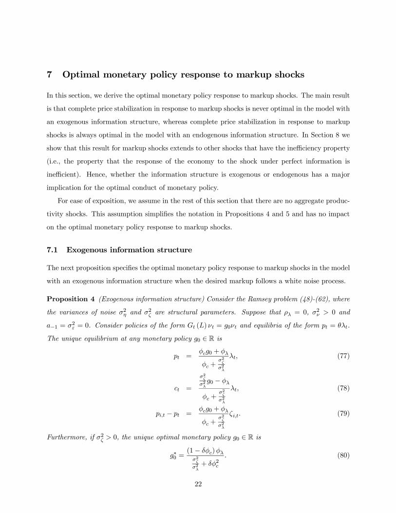
7.1 Exogenous information structure

The next proposition specifies the optimal monetary policy response to markup shocks in the model

with an exogenous information structure when the desired markup follows a white noise process.

Proposition 4 (Exogenous information structure) Consider the Ramsey problem (48)-(62), where

the variances of noise σ2η and σ2ζ are structural parameters. Suppose that ρλ = 0, σ2ν > 0 and

a−1 = σ2ε = 0. Consider policies of the form Gt (L) νt = g0νt and equilibria of the form pt = θλt.

The unique equilibrium at any monetary policy g0 ∈ R is

pt =φcg0 + φλ

φc +σ2ζσ2λ

λt, (77)

ct =

σ2ζσ2λg0 − φλ

φc +σ2ζσ2λ

λt, (78)

pi,t − pt =φcg0 + φλ

φc +σ2ζσ2λ

ζi,t. (79)

Furthermore, if σ2ζ > 0, the unique optimal monetary policy g0 ∈ R is

g∗0 =(1− δφc)φλσ2ζσ2λ+ δφ2c

. (80)

22

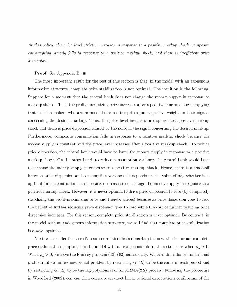
At this policy, the price level strictly increases in response to a positive markup shock, composite

consumption strictly falls in response to a positive markup shock, and there is inefficient price

dispersion.

Proof. See Appendix B.

The most important result for the rest of this section is that, in the model with an exogenous

information structure, complete price stabilization is not optimal. The intuition is the following.

Suppose for a moment that the central bank does not change the money supply in response to

markup shocks. Then the profit-maximizing price increases after a positive markup shock, implying

that decision-makers who are responsible for setting prices put a positive weight on their signals

concerning the desired markup. Thus, the price level increases in response to a positive markup

shock and there is price dispersion caused by the noise in the signal concerning the desired markup.

Furthermore, composite consumption falls in response to a positive markup shock because the

money supply is constant and the price level increases after a positive markup shock. To reduce

price dispersion, the central bank would have to lower the money supply in response to a positive

markup shock. On the other hand, to reduce consumption variance, the central bank would have

to increase the money supply in response to a positive markup shock. Hence, there is a trade-off

between price dispersion and consumption variance. It depends on the value of δφc whether it is

optimal for the central bank to increase, decrease or not change the money supply in response to a

positive markup shock. However, it is never optimal to drive price dispersion to zero (by completely

stabilizing the profit-maximizing price and thereby prices) because as price dispersion goes to zero

the benefit of further reducing price dispersion goes to zero while the cost of further reducing price

dispersion increases. For this reason, complete price stabilization is never optimal. By contrast, in

the model with an endogenous information structure, we will find that complete price stabilization

is always optimal.

Next, we consider the case of an autocorrelated desired markup to know whether or not complete

price stabilization is optimal in the model with an exogenous information structure when ρλ > 0.

When ρλ > 0, we solve the Ramsey problem (48)-(62) numerically. We turn this infinite-dimensional

problem into a finite-dimensional problem by restricting Gt (L) to be the same in each period and

by restricting Gt (L) to be the lag-polynomial of an ARMA(2,2) process. Following the procedure

in Woodford (2002), one can then compute an exact linear rational expectations equilibrium of the

23

model (49)-(62) for a given monetary policy by solving a Riccati equation. We then run a numerical

optimization routine to obtain the optimal monetary policy.5

Figure 1 shows the optimal monetary policy response to a markup shock in the model with

an exogenous information structure for the following parameter values: β = 0.99, γ = 1, ψ = 0,

α = (2/3), Λ = (1/3), σν = 0.2, and σζ = 0.4. The upper panel of Figure 1 shows optimal monetary

policy in the case of ρλ = 0. The lower panel of Figure 1 shows optimal monetary policy in the case

of ρλ = 0.9. For comparison, Figure 1 also shows optimal monetary policy in the Calvo model with

perfect information and an average price duration of 2.5 quarters. The parameter value Λ = (1/3)

implies a steady-state price elasticity of demand of four, which is within the range of estimates of the

price elasticity of demand in the Industrial Organization literature. The parameter values ρλ = 0.9

and σν = 0.2 are within the range of estimates of markup shocks in the New Keynesian literature.

The Calvo parameter is taken from Nakamura and Steinsson (2008). The standard deviation of

noise is set such that the model with imperfect information and the Calvo model yield the same

response of the price level to a markup shock when the component of the profit-maximizing price

driven by markup shocks is a random walk. The idea is that we aim to compare the model with

imperfect information and the Calvo model for parameter values that imply the same degree of

stickiness of the price level. All impulse responses are to a positive one standard deviation markup

shock. A response equal to one means a one percent deviation from the non-stochastic steady state.

Time is measured in quarters along the horizontal axis.

We obtain the following results. First of all, in the model with an exogenous information struc-

ture, complete price stabilization is still suboptimal when ρλ > 0. At the optimal monetary policy,

the price level strictly increases on impact of a positive markup shock and composite consumption

strictly falls on impact of a positive markup shock. Figure 1 shows this result for our benchmark

parameter values. We solved the Ramsey problem (48)-(62) for many sets of parameter values with

ρλ > 0 and we always obtained this result. Second, whether the optimal monetary policy response

to markup shocks is similar in the model with exogenous imperfect information and in the Calvo

model depends on ρλ. When ρλ = 0.9, we find that optimal monetary policy is roughly the same

in the two models. When ρλ = 0, optimal monetary policy is quite different in the two models.

5We choose an ARMA(2,2) parameterization because it is well known from time series econometrics that an

ARMA(p,q) parameterization is a very flexible and parsimonious parameterization.

24

Specifically, when ρλ = 0, the optimal policy in the model with exogenous imperfect information

is to respond to the markup shock only in the period of the shock, while the optimal policy in the

Calvo model is to respond to the markup shock also in the periods after the shock. The reason

is the following. In the model with exogenous imperfect information, firms set prices period by

period implying: (i) future monetary policy has no effect on today’s price setting, and (ii) when

ρλ = 0 today’s markup shock creates no inefficiencies in future periods so long as the central bank

does not respond to today’s markup shock in future periods. Hence, when ρλ = 0, the optimal

monetary policy in the model with exogenous imperfect information is to respond to the markup

shock only in the period of the shock. In the Calvo model, price setting is forward looking and firms

adjusting prices today but not tomorrow carry the markup shock forward. For these reasons, even

when ρλ = 0, the optimal monetary policy in the Calvo model is to respond to the markup shock

also in the periods after the shock. Despite these differences between the model with exogenous

imperfect information and the Calvo model, the optimal monetary policy is roughly the same in

the two models when ρλ = 0.9. We think this is an interesting result, but this is not the main

result of this paper. We now turn to the main result of this paper.

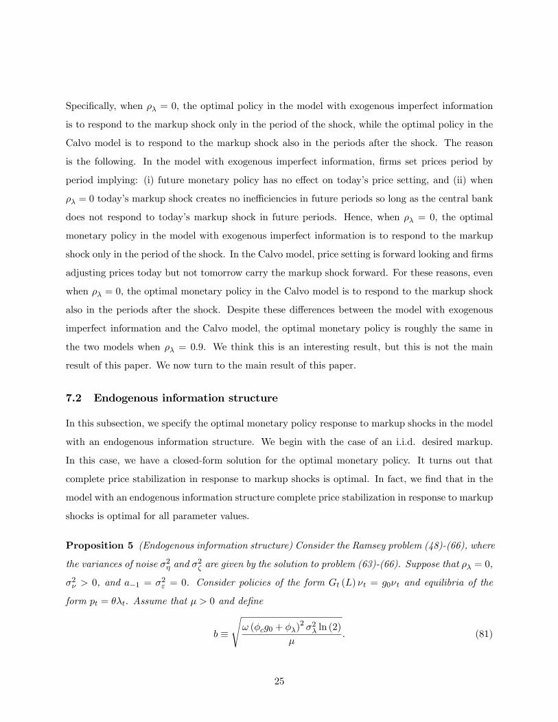
7.2 Endogenous information structure

In this subsection, we specify the optimal monetary policy response to markup shocks in the model

with an endogenous information structure. We begin with the case of an i.i.d. desired markup.

In this case, we have a closed-form solution for the optimal monetary policy. It turns out that

complete price stabilization in response to markup shocks is optimal. In fact, we find that in the

model with an endogenous information structure complete price stabilization in response to markup

shocks is optimal for all parameter values.

Proposition 5 (Endogenous information structure) Consider the Ramsey problem (48)-(66), where

the variances of noise σ2η and σ2ζ are given by the solution to problem (63)-(66). Suppose that ρλ = 0,

σ2ν > 0, and a−1 = σ2ε = 0. Consider policies of the form Gt (L) νt = g0νt and equilibria of the

form pt = θλt. Assume that μ > 0 and define

b ≡

sω (φcg0 + φλ)

2 σ2λ ln (2)

μ. (81)

25

First, we characterize the set of equilibria at a given monetary policy g0 ∈ R. Here κ∗ is the

equilibrium attention devoted to the desired markup. If and only if b ≤ 1, there exists an equilibrium

with

κ∗ = 0. (82)

If and only if either φc ∈¡0, 12

¤and b ≥

p4φc (1− φc) or φc > 1

2 and b ≥ 1, there exists an

equilibrium with

κ∗ = log2

Ãb+

pb2 − 4φc (1− φc)

2φc

!. (83)

If and only if φc ∈¡0, 12

¤and b ∈

hp4φc (1− φc), 1

i, there exists an equilibrium with

κ∗ = log2

Ãb−

pb2 − 4φc (1− φc)

2φc

!. (84)

The equilibrium price level, composite consumption, and price dispersion are given by

pt =(φcg0 + φλ)

¡1− 2−2κ∗

¢1− (1− φc) (1− 2−2κ

∗)λt, (85)

ct =

"g0 −

(φcg0 + φλ)¡1− 2−2κ∗

¢1− (1− φc) (1− 2−2κ

∗)

#λt, (86)

and

Eh(pi,t − pt)

2i=

μω

ln (2)

³1− 2−2κ∗

´. (87)

Second, we characterize optimal monetary policy. If φc ∈£12 ,∞

¢, there exists a unique equilibrium

for any monetary policy g0 ∈ R and the unique optimal monetary policy is

g∗0 =

⎧⎨⎩ 0 if ωφ2λσ2λ ln(2)μ ≤ 1

−φλφc+ 1

φc

qμ

ωσ2λ ln(2)if ωφ2λσ

2λ ln(2)μ > 1

. (88)

At this policy, decision-makers in firms who set prices devote no attention to the desired markup,

and the price level does not respond to markup shocks.

Proof. See Appendix C.

The main result in Proposition 5 is that in the model with an endogenous information structure

complete price stabilization in response to markup shocks is optimal when ρλ = 0, μ > 0, and

φc ∈£12 ,∞

¢. The condition ρλ = 0 means that the desired markup follows a white noise process.

The condition μ > 0 means that there is some cost of devoting attention to the desired markup

26

(this cost can be arbitrarily small or arbitrarily large). The condition φc ∈£12 ,∞

¢means that

strategic complementarity in price setting is not so large such that there are multiple equilibria.

Below we show analytically that in the case of an i.i.d. desired markup complete price stabilization

in response to markup shocks is also optimal when μ = 0 or φc ∈¡0, 12

¢. Hence, in the case of an

i.i.d. desired markup complete price stabilization in response to markup shocks is always optimal in

the model with an endogenous information structure. This result is in the starkest possible contrast

to Proposition 4 stating that in the case of an i.i.d. desired markup complete price stabilization in

response to markup shocks is never optimal in the model with an exogenous information structure.

To understand Proposition 5, let us first understand the optimal allocation of attention by

decision-makers in firms because this is the new feature in the model with an endogenous informa-

tion structure. The profit-maximizing price of good i in period t equals

p∗i,t = (1− φc) pt + φcmt − φaat + φλλt

= [(1− φc) θ + φcg0 + φλ]λt. (89)

To find out about the current value of the profit-maximizing price, the decision-maker in firm i can

pay attention to the desired markup. We let decision-makers in firms choose themselves how much

attention they want to devote to the desired markup. The optimal attention devoted to the desired

markup equals

κ∗ =

⎧⎨⎩12 log2

³ω[(1−φc)θ+φcg0+φλ]2σ2λ ln(2)

μ

´if ω[(1−φc)θ+φcg0+φλ]2σ2λ ln(2)

μ ≥ 1

0 otherwise. (90)

The ratio ω[(1−φc)θ+φcg0+φλ]2σ2λ ln(2)μ is the marginal benefit of paying attention to the desired markup

at no attention devoted to the desired markup (κ = 0) divided by the marginal cost of paying

attention to the desired markup. If this ratio exceeds one, the decision-maker pays some attention

to the desired markup. If this ratio increases, the decision-maker pays more attention to the

desired markup, which raises the signal-to-noise ratio in the signal concerning the desired markup.

The benefit of paying attention to the desired markup depends on the variance of the profit-

maximizing price due to the desired markup: [(1− φc) θ + φcg0 + φλ]2 σ2λ. This variance in turn

depends on the behavior of other firms through θ and on monetary policy through g0. In particular,

as pointed out by Mackowiak and Wiederholt (2009) and Hellwig and Veldkamp (2009), strategic

complementarity in price setting leads to strategic complementarity in the allocation of attention.

27

When other firms are paying more attention to the desired markup, the price level responds more

to the desired markup, which in the case of (1− φc) > 0 raises the incentive for an individual firm

to pay attention to the desired markup. For this reason, multiple equilibria can in principle arise.

However, when φc ∈£12 ,∞

¢, strategic complementarity in price setting is not strong enough for

multiple equilibria to arise. In this case, if the compound parameter b defined by equation (81)

is below one, the unique equilibrium attention is given by equation (82); while if the compound

parameter b is above one, the unique equilibrium attention is given by equation (83). To illustrate

this result, the upper panel of Figure 2 shows equilibrium attention as a function of the compound

parameter b for φc = (1/2). By contrast, when φc ∈¡0, 12

¢, strategic complementarity in price

setting is strong enough for multiple equilibria to arise at some values of the compound parameter

b. To illustrate this result, the lower panel of Figure 2 shows equilibrium attention as a function of

the compound parameter b for φc = (1/4).

Let us now turn to optimal monetary policy. Proposition 5 specifies optimal monetary policy

when φc ∈£12 ,∞

¢and thus there exists a unique equilibrium for any monetary policy g0 ∈ R.

First, consider the case of ωφ2λσ2λ ln(2)μ ≤ 1. In this case, if the central bank does not respond to

markup shocks (i.e., g0 = 0), decision-makers in firms pay no attention to markup shocks because

the marginal benefit of paying attention to random variation in the desired markup is smaller than

the marginal cost of paying attention to random variation in the desired markup. Moreover, when

neither the central bank nor firms respond to markup shocks, markup shocks create no inefficiencies.

Hence, in the case of ωφ2λσ

2λ ln(2)μ ≤ 1, a monetary policy of no response to markup shocks implements

the efficient allocation and is therefore the optimal monetary policy. Second, consider the case ofωφ2λσ

2λ ln(2)μ > 1. In this case, if the central bank does not respond to markup shocks (i.e., g0 = 0),

decision-makers in firms do pay attention to markup shocks because the marginal benefit of paying

attention to random variation in the desired markup exceeds the marginal cost of paying attention

to random variation in the desired markup. Hence, in the case of ωφ2λσ2λ ln(2)μ > 1, if the central

bank does not respond to markup shocks, the price level increases after a positive markup shock,

composite consumption falls after a positive markup shock, and there is price dispersion caused by

the noise in the signal concerning the desired markup. Suppose instead that the central bank lowers

the money supply after a positive markup shock (i.e., g0 < 0). Recall first what happens in the

model with an exogenous information structure: when the central bank lowers the money supply

28

after a positive markup shock, price dispersion falls (because the profit-maximizing price increases

by less after a positive markup shock implying that firms put less weight on their noisy signals)

and consumption variance increases (because the reduction in the money supply after a positive

markup shock amplifies the fall in consumption after a positive markup shock). Hence, there is a

trade-off between price dispersion and consumption variance. Next return to the model with an

endogenous information structure. In this model, there is one additional effect. When the central

bank lowers the money supply after a positive markup shock, the profit-maximizing price increases

by less after a positive markup shock, implying that the variance of the profit-maximizing price due

to markup shocks falls. Decision-makers in firms pay less attention to markup shocks. Due to this

one additional effect, the trade-off between price dispersion and consumption variance disappears.

Think about consumption variance. On the one hand, the reduction in the money supply after a

positive markup shock by itself amplifies the fall in consumption after a positive markup shock.

On the other hand, the fact that decision-makers in firms are now paying less attention to markup

shocks implies that the price level increases less after a positive markup shock, which by itself

reduces the fall in consumption after a positive markup shock. It turns out that the second effect

(less attention devoted to markup shocks) dominates for all parameter values. A monetary policy of

reducing the money supply after a positive markup shock therefore reduces consumption variance.

It discourages decision-makers in firms from paying attention to random variation in the desired

markup. For this reason, the trade-off between price dispersion and consumption variance (which

is a classic result in monetary economics) disappears. It is now straightforward to derive optimal

monetary policy. So long as decision-makers in firms are paying some attention to markup shocks,

the central bank can lower both price dispersion and consumption variance by counteracting the

markup shock more strongly and thereby reducing the variance of the profit-maximizing price due

to markup shocks. Once decision-makers in firms are paying no attention to markup shocks, price

dispersion equals zero and reducing the money supply even further after a positive markup shock

would only increase consumption variance. Hence, the optimal monetary policy is the one that

makes decision-makers in firms just pay no attention to markup shocks. The lower part of equation

(88) specifies this policy. At this policy, decision-makers in firms are paying no attention to markup

shocks and thus prices do not respond to markup shocks. Complete price stabilization in response

to markup shocks is optimal.

29

Figure 3 illustrates Proposition 5 for the following parameter values: γ = 1, ψ = 0, α = (2/3),

Λ = (1/3), ρλ = 0, and σ2λ =h(0.2)2 /

³1− (0.9)2

´i. Figure 3 depicts price setters’ equilibrium

attention devoted to markup shocks (κ∗) at the optimal monetary policy, the optimal monetary

policy (g∗0), and the loss in welfare due to markup shocks at the optimal monetary policy for

different values of (μ/ω). Recall that μ > 0 is the per-period marginal cost of attention of the

decision-maker in a firm and ω > 0 is the constant in the price setters’ objective (63).

Proposition 5 specifies optimal monetary policy when φc ∈£12 ,∞

¢, that is, when strategic

complementarity in price setting is not large enough for multiple equilibria to arise. Proposition

6 specifies optimal monetary policy when φc ∈¡0, 12

¢, that is, when strategic complementarity in

price setting is large enough for multiple equilibria to arise at some monetary policies g0 ∈ R.

Before one can make a statement about optimal monetary policy in this case, one has to make

an assumption about the central bank’s attitude towards multiple equilibria. The most common

assumption in the literature seems to be that central banks are very adverse to multiple equilibria.

Therefore, we assume that the central bank aims to implement the best policy among all those

monetary policies g0 ∈ R that yield a unique equilibrium.

Proposition 6 (Endogenous information structure) Consider the Ramsey problem (48)-(66), where

the variances of noise σ2η and σ2ζ are given by the solution to problem (63)-(66). Suppose that ρλ = 0,

σ2ν > 0, and a−1 = σ2ε = 0. Consider policies of the form Gt (L) νt = g0νt and equilibria of the

form pt = θλt. Assume that μ > 0. If φc ∈¡0, 12

¢, there exist multiple equilibria for all g0 ∈ [g0, g0]

where

g0 = −φλφc+

p4φc (1− φc)

φc

rμ

ωσ2λ ln (2), (91)

and

g0 = −φλφc+1

φc

rμ

ωσ2λ ln (2). (92)

If ωφ2λσ2λ ln(2)μ < 4φc (1− φc), the best policy among all g0 ∈ R that yield a unique equilibrium

is g∗0 = 0. If ωφ2λσ2λ ln(2)μ ≥ 4φc (1− φc), the best policy among all g0 ∈ R that yield a unique

equilibrium is a g0 marginally below g0. At this policy, decision-makers in firms who set prices

devote no attention to the desired markup, and the price level does not respond to markup shocks.

Proof. See Appendix C.

30

The main result in Proposition 6 is that in the model with an endogenous information structure

complete price stabilization in response to markup shocks is also optimal when φc ∈¡0, 12

¢. To

understand this result, note the following. When g0 ∈ [g0, g0], the compound parameter b governing

the benefit to the cost of paying attention to markup shocks lies in the intervalhp4φc (1− φc), 1

i.

Furthermore, the first half of Proposition 5 states that, if φc ∈¡0, 12

¢and b ∈

hp4φc (1− φc), 1

i,

then multiple equilibria arise. See Figure 2 for an illustration. Hence, if φc ∈¡0, 12

¢, the central bank

has to choose g0 /∈ [g0, g0] to avoid multiple equilibria. Next, think about optimal monetary policy.

When ωφ2λσ2λ ln(2)μ < 4φc (1− φc) we have g0 > 0. Thus, at the policy g0 = 0, κ∗ = 0 is the unique

equilibrium. When the central bank and firms do not respond to markup shocks, those shocks create

no inefficiencies. Hence, in the case of ωφ2λσ2λ ln(2)μ < 4φc (1− φc), a monetary policy of no response

to markup shocks is the optimal monetary policy. By contrast, when ωφ2λσ2λ ln(2)μ ≥ 4φc (1− φc) we

have g0 ≤ 0. Thus, at the policy g0 = 0, κ∗ = 0 is not the unique equilibrium. To understand

optimal monetary policy in this case, consider the lower panel of Figure 2. When g0 > g0 and thus

b > 1, both price dispersion and consumption variance fall when the central bank reduces g0 for the

same reasons given below Proposition 5. When g0 < g0 and thus b <p4φc (1− φc), consumption

variance falls when the central bank increases g0. Finally, the no attention equilibrium at g0 = g0

strictly dominates the high positive attention equilibrium at g0 = g0. Hence, the best policy among

all policies that yield a unique equilibrium is a g0 marginally below g0. At this policy, decision-

makers in firms who set prices pay no attention to random variation in the desired markup, and

prices do not respond to markup shocks. Complete price stabilization in response to markup shocks

is optimal.

Finally, we consider the case of an autocorrelated desired markup. When ρλ > 0, we solve the

Ramsey problem (48)-(66) numerically. Figure 4 shows the optimal monetary policy response to a

markup shock in the model with an endogenous information structure for the following parameter

values: β = 0.99, γ = 1, ψ = 0, α = (2/3), Λ = (1/3), ρλ = 0.9, and σν = 0.2. At the optimal

monetary policy, decision-makers in firms who set prices devote no attention to random variation

in the desired markup, and the price level does not respond to markup shocks. Complete price

stabilization in response to markup shocks is optimal. We solved the Ramsey problem (48)-(66)

for many sets of parameter values with ρλ > 0 and we always obtained this result.

31

8 Additional results and robustness of the main results

In this section, we present two additional results for the model with an endogenous information

structure (Sections 8.1-8.2). Furthermore, we show that our main conclusions are robust to several

modifications of the model with an endogenous information structure (Sections 8.3-8.6). Here

we want to highlight two results. First, optimal monetary policy remains the same when decision-

makers in firms can decide to receive signals concerning any linear combination of at and λt. Second,

the optimality of complete price stabilization extends from markup shocks to a much larger class

of shocks.

8.1 Welfare at the optimal monetary policy

We now study how welfare at the optimal monetary policy varies with the parameters governing

the degree of information friction. These parameters are: the marginal cost of attention in the

model with an endogenous information structure, μ, and the variances of noise in the model with

an exogenous information structure, σ2η and σ2ζ .

In the model with an endogenous information structure and ρλ = 0, the value of the central

bank’s objective (48) at the optimal policy specified in Propositions 3, 5, and 6 equals

∞Xt=0

βtE

"(ct − c∗t )

2 + δ1

I

IXi=1

(pi,t − pt)2

#=

1

1− β(g∗0)

2 σ2λ, (93)

where g∗0 is given by Proposition 5 if φc ∈£12 ,∞

¢and g∗0 is given by Proposition 6 if φc ∈

¡0, 12

¢.

The loss in welfare relative to the efficient allocation is weakly decreasing in μ because the absolute

value of g∗0 is weakly decreasing in μ. See Figure 3 for an illustration. The intuition is simple. When

price setters’ marginal cost of paying attention to markup shocks is larger, the central bank does

not have to counteract markup shocks as much to discourage price setters from paying attention

to these shocks that cause inefficient fluctuations.

In the model with an exogenous information structure and ρλ = 0, the value of the central

bank’s objective (48) at the optimal policy specified in Propositions 2 and 4 equals

∞Xt=0

βtE

"(ct − c∗t )

2 + δ1

I

IXi=1

(pi,t − pt)2

#=

1

1− β

⎡⎢⎣⎛⎜⎝ δφcφλ

σ2ζσ2λ+ δφ2c

⎞⎟⎠2

σ2λ + δ

⎛⎜⎝ φλσ2ζσ2λ+ δφ2c

⎞⎟⎠2

σ2ζ

⎤⎥⎦ .(94)

32

The loss in welfare relative to the efficient allocation is decreasing in the variance of noise σ2ζ .

A larger variance of noise decreases inefficient consumption fluctuations because prices respond

less strongly to markup shocks. On the other hand, a larger variance of noise may increase price

dispersion because the signal concerning the desired markup is more noisy. It turns out that the

first effect dominates, that is, the derivative of expression (94) with respect to σ2ζ is strictly negative.

Hence, the loss in welfare is decreasing in σ2ζ .

In summary, in the model with an endogenous information structure easier access to informa-

tion concerning markup shocks reduces welfare, and in the model with an exogenous information

structure a more precise private signal concerning markup shocks reduces welfare. The reason is

that markup shocks cause inefficient consumption fluctuations.6

8.2 The value of commitment

It is well understood that in the Calvo model there is a value of commitment to future monetary

policy when there are markup shocks. By contrast, in the model with exogenous imperfect infor-

mation, there is no value of commitment to future monetary policy because firms set prices period

by period. Finally, in the model with an endogenous information structure, there is a value of

commitment to future monetary policy when there are markup shocks and g∗0 < 0. The reason

is the following. In this case, only when the central bank can commit, price setters can trust the

central bank that not paying attention to aggregate conditions is optimal. We find it interesting

that the nature of the value of commitment in the rational inattention model is different from the

nature of the value of commitment in the Calvo model.

8.3 More general signal structure

We have so far assumed that paying attention to aggregate productivity and paying attention

to the desired markup are independent activities. Formally, in equation (55) we assume that the

decision-maker in firm i who has to set a price receives two independent signals concerning aggregate

productivity and the desired markup. The interpretation of this assumption is that paying attention

to aggregate productivity and paying attention to the desired markup are independent activities.

6Baeriswyl and Cornand (2010) also argue that information about markup shocks is harmful. They study a model

with an exogenous information structure.

33

We now relax this assumption. We assume that the decision-maker in firm i who has to set a price

can pay attention to any variable that is a linear combination of at and λt. Formally, the signal

that the price setter of good i receives in period t can be any signal of the form

si,t = ξaat + ξλλt + ζi,t. (95)

In the new model with an endogenous information structure, the decision-maker in firm i chooses

the coefficients (ξa, ξλ) ∈ R2 and the variance of noise σ2ζ ∈ R+.7 We interpret the choice of (ξa, ξλ)

as the choice of which variable to pay attention to (e.g., ξa and ξλ could be chosen such that

ξaat+ ξλλt equals the equilibrium price level or equilibrium consumption). We interpret the choice

of σ2ζ as the choice of how much attention to devote to this variable.

For the old signal structure (55), the information flow constraint (20) reduces to equation (65).

For the new signal structure (95), this is no longer the case and we therefore have to work with

the original formulation of the information flow constraint (20). Hence, in the new model with

an endogenous information structure, the Ramsey problem (48)-(66) changes as follows. Equation

(95) replaces equation (55), equation (20) replaces equation (65), and the decision-maker in firm i

chooses³ξa, ξλ, 1/σ

2ζ

´rather than

³1/σ2η, 1/σ

2ζ

´.

In the case of ρa = ρλ = 0, we can solve this new Ramsey problem analytically. In particular,

the optimal monetary policy is again the monetary policy specified in Propositions 3, 5, and 6.

The reason is quite simple. When ρa = ρλ = 0, the optimal signal is a signal concerning the

profit-maximizing price, that is, the optimal choice of (ξa, ξλ) is the (ξa, ξλ) with the property

that ξaat+ ξλλt equals the equilibrium profit-maximizing price. In addition, the optimal attention

devoted to the profit-maximizing price equals

κ∗ =

⎧⎪⎨⎪⎩12 log2

µωσ2

p∗ ln(2)

μ

¶if

ωσ2p∗ ln(2)

μ ≥ 1

0 otherwise, (96)

where σ2p∗ is the variance of the profit-maximizing price. The signal-to-noise ratio then equals

σ2p∗

σ2ζ= 22κ

∗ − 1, (97)

and the price set by firm i in period t equals

pi,t = E£p∗i,t|Ii,t

¤=³1− 2−2κ∗

´ ¡p∗i,t + ζi,t

¢. (98)

7Adam (2007) and Mondria (2010) model the attention decision in a similar way.

34

Let us now turn to optimal monetary policy. First, consider the monetary policy response to

aggregate productivity shocks. Suppose that the central bank commits to the monetary policy

specified in Proposition 3. This policy yields the efficient response of composite consumption to

aggregate productivity shocks. Furthermore, this policy yields a variance of the profit-maximizing

price due to aggregate productivity shocks of zero. Thus, this policy is the monetary policy response

to aggregate productivity shocks that yields the smallest κ∗ and the smallest price dispersion.

Moreover, a small κ∗ is good because then prices respond less to markup shocks. For these reasons,

the optimal monetary policy response to aggregate productivity shocks is the monetary policy

specified in Proposition 3. Second, once the profit-maximizing price does not respond to aggregate

productivity shocks, equation (96) reduces to equation (90). In other words, the firms’ optimal

allocation of attention is exactly the same as in the model with no aggregate productivity shocks.

For this reason, the optimal monetary policy response to markup shocks is the monetary policy

specified in Propositions 5 and 6.

8.4 More general shocks

We have so far studied two types of shocks: aggregate productivity shocks and markup shocks. We

now show that the results from Sections 6 and 7 extend to a much larger class of shocks. Consider

a more general exogenous variable zt that may affect both efficient composite consumption and the

profit-maximizing price:

c∗t = ϕzt, (99)

and

p∗i,t = pt + φcct + φzzt, (100)

where ϕ ∈ R, φz ∈ R++, and zt follows a stationary Gaussian first-order autoregressive process.

Two examples of the exogenous variable zt are aggregate productivity and the desired markup.

If zt = −at then φz = φa and ϕ = − (φa/φc). If zt = λt then φz = φλ and ϕ = 0. Apart

from introducing a more general exogenous variable by replacing equations (49) and (53) by (99)

and (100), the Ramsey problem (48)-(66) remains unchanged.8 In particular, each price setter

chooses the precision of his/her signal knowing that a more precise signal requires more attention.

8For clarity of exposition, we now assume in equations (99)-(100) that there is only one exogenous variable.

35

Formally, si,t = zt + ηi,t and κ = 12 log2

Ãσ2z|st−1

i

σ2z|st

i

!. What is the optimal monetary policy response

to an innovation in zt?

First, note that if decision-makers in firms had perfect information then each firm would set

the profit-maximizing price, implying that

ct = −φzφc

zt, (101)

and

pi,t − pt = 0. (102)

Second, consider the case of −φzφc= ϕ. In this case, a z shock (i.e., an innovation in zt) has the

efficiency property: the response of the economy to a z shock under perfect information is efficient.

Then, the reasoning of Sections 5 and 6 applies. By setting mt = c∗t the central bank can replicate

the perfect-information response of the economy to a z shock and this response is efficient. Hence,

in the case of −φzφc= ϕ, the optimal monetary policy response to a z shock is given by mt = c∗t .

One example of a z shock with the property −φzφc= ϕ is an aggregate productivity shock in the

model given in Section 2.

Third, consider the case of −φzφc

< ϕ. In this case, a z shock has the inefficiency property: the

response of the economy to a z shock under perfect information is inefficient. More precisely, either

the response of actual consumption and the response of efficient consumption have the same sign

but the response of actual consumption is larger in magnitude (i.e., −φzφc

< ϕ ≤ 0) or the response of

actual consumption and the response of efficient consumption have the opposite sign (i.e., ϕ > 0).

One example of a z shock with the property −φzφc

< ϕ is a markup shock in the model given

in Section 2 because the response of equilibrium consumption to a markup shock under perfect

information is larger in magnitude than the response of efficient consumption to a markup shock.

It turns out that Proposition 5 generalizes in a straightforward way from markup shocks to any z

shock with the property −φzφc

< ϕ. In the beginning of the new proposition it says ρz = 0, σ2z > 0,

mt = g0zt, and pt = θzt. The only change in equations (81)-(87) is that φz and σ2z replace φλ and

σ2λ. Furthermore, equation (88) becomes

g∗0 =

⎧⎨⎩ ϕ if ω(φcϕ+φz)2σ2z ln(2)

μ ≤ 1

−φzφc+ 1

φc

qμ

ωσ2z ln(2)if ω(φcϕ+φz)

2σ2z ln(2)μ > 1

. (103)

36

Most importantly, at the optimal monetary policy, decision-makers in firms who set prices devote

no attention to the variable zt, and the price level does not respond to an innovation in zt. Hence,

in the model with an endogenous information structure, complete price stabilization is optimal in

response to any z shock with the property −φzφc

< ϕ.

Finally, consider the case of ϕ < −φzφc. In this case, the response of actual consumption and the

response of efficient consumption have the same sign but the response of efficient consumption is

larger in magnitude. The proof of Proposition 5 does not generalize in a straightforward way from

markup shocks to this case. Therefore, we do not know yet whether complete price stabilization is

optimal in response to z shocks with the property ϕ < −φzφc. This may or may not be the case.

In summary, our result of complete price stabilization extends from aggregate productivity

shocks (i.e., −φzφc= ϕ) and markup shocks (i.e., ϕ = 0) to any z shock with the property −φz

φc≤ ϕ

(i.e., any z shock with the property that equilibrium fluctuations under perfect information equal,

are larger in magnitude, or have the opposite sign than efficient fluctuations).

8.5 Information of the central bank

So far we did not model the information choice of the central bank. We simply assumed that the

central bank has perfect information and can therefore implement the optimal monetary policy.

We now study the central bank’s benefit of learning aggregate conditions. If the central bank

has no information about aggregate conditions, the central bank cannot respond to aggregate

productivity shocks and markup shocks. Figure 5 shows the central bank’s benefit of learning

aggregate conditions for the following parameter values: γ = 1, ψ = 0, α = (2/3), Λ = (1/3),

ρa = ρλ = 0, σ2a =

h(0.0085)2 /

³1− (0.95)2

´iand σ2λ =

h(0.2)2 /

³1− (0.9)2

´i.9 In particular, the

upper panel shows the loss in welfare (compared to the efficient allocation) in the case of the optimal

monetary policy response to aggregate productivity shocks and in the case of no policy response to

aggregate productivity shocks. The lower panel of Figure 5 shows the loss in welfare (compared to

the efficient allocation) in the case of the optimal monetary policy response to markup shocks and

in the case of no policy response to markup shocks. For values of (μ/ω) between 0.1 ∗ 10−3 and9The parameter values ρa = 0.95 and σε = 0.0085 are a standard calibration of the aggregate productivity process.

We set ρa = 0 and σ2a = (0.0085)2 / 1− (0.95)2 to make Figure 5 comparable to Figure 3. The figure looks similar

for ρa = 0.95 and σε = 0.0085, which again implies σ2a = (0.0085)2 / 1− (0.95)2 .

37

0.9∗10−3, the per-period welfare gain from implementing the optimal monetary policy is quite large:

about half a percent of steady state consumption.10 Hence, for these values of (μ/ω), the central

bank has a substantial incentive to become informed about aggregate conditions to implement the

optimal monetary policy. At the same time, this optimal monetary policy makes the variance of the

profit-maximizing price due to aggregate shocks sufficiently small such that price setters in firms

pay no attention to aggregate conditions.11

Furthermore, the central bank does not literally have to know aggregate productivity and the

desired markup. Suppose that the central bank knows output, the output gap and the price level,

where the output gap is defined as output minus efficient output. The central bank can then

implement a monetary policy that is arbitrarily close to the optimal monetary policy. The idea is

simple: if the central bank encourages firms to pay a little bit of attention to the desired markup, the

price level reveals the desired markup to the central bank and nevertheless the loss in welfare due

to deviations from the optimal monetary policy can be made arbitrarily small. Formally, consider

the case of ρλ = 0, φc ∈£12 ,∞

¢, and ωφ2λσ

2λ ln(2)μ > 1.12 Suppose that the central bank implements

the following monetary policy

mt = c∗t + g01− (1− φc)

¡1− 2−2κ∗

¢(φcg0 + φλ) (1− 2−2κ

∗)pt. (104)

Here c∗t is efficient composite consumption, g0 ∈ (g∗0, 0) where g∗0 is given by equation (88), κ∗ is

given by equations (81) and (83), and the ratio in front of the price level is the inverse of the ratio

in equation (85). Since g0 > g∗0, price setters pay some attention to markup shocks and the price

level reveals the desired markup to the central bank. At the same time, by making the difference

g0−g∗0 arbitrarily small, the central bank can approximate the optimal monetary policy arbitrarily

well.10Mackowiak and Wiederholt (2010) solve a DSGE model with rational inattention and a Taylor rule. They find

that for a value of (μ/ω) between 0.1 ∗ 10−3 and 0.2 ∗ 10−3 the model matches various empirical impulse responses

of prices to shocks.11 In the welfare calculations, we are not taking into account that the optimal monetary policy has additional welfare

benefits due to the fact that price setters do not have to pay attention to aggregate conditions and can thus focus on

firm-specific conditions. Taking these additional welfare benefits into account would strengthen the case for complete

price stabilization in response to aggregate shocks and would increase the welfare gain from optimal monetary policy.12The case ωφ2λσ

2λ ln(2)

μ> 1 is the interesting case, because when ωφ2λσ

2λ ln(2)

μ≤ 1 the central bank needs no informa-

tion about the desired markup to implement the optimal policy. See Proposition 5.

38

In the New Keynesian literature on optimal monetary policy, it is typically assumed that the

central bank knows the output gap and inflation, where the output gap is defined as output minus

efficient output. See for example Woodford (2003), Chapter 8, and Giannoni and Woodford (2010).

Thus, when we assume that the central bank knows output, the output gap and the price level,

we make essentially the same assumption about information of the central bank as the standard

New Keynesian literature. Despite this, we obtain a markedly different result concerning optimal

monetary policy: the optimal monetary policy is arbitrarily close to complete price stabilization in

response to markup shocks and the only purpose of arbitrarily small fluctuations in the price level

is to reveal the desired markup to the central bank.

We think it would be interesting to study optimal monetary policy when the central bank only

observes noisy indicators of the output gap and inflation. Svensson and Woodford (2003, 2004)

study this question in a New Keynesian model and Lorenzoni (2010) studies this question in a model

with exogenous dispersed information. For studying this question, it will be useful to know what

the central bank should do when the central bank has perfect information, which is the content of

this paper.

8.6 Interest rate rule

We now assume that the central bank commits to an interest rate rule, rather than a money supply

rule. Assuming that the central bank can commit to an interest rate rule of the form (11) instead

of a money supply rule of the form (10) does not affect optimal monetary policy. This is because

the set of equilibria that the central bank can implement with an interest rate rule of the form (11)

equals the set of equilibria that the central bank can implement with a money supply rule of the form

(10). To see this, note the following. We so far did not use the log-linearized consumption Euler

equation in the Ramsey problem (48)-(66) because in the case of a money supply rule this equation

only determines the equilibrium nominal interest rate. Now take a law of motion of the economy

that is an equilibrium law of motion under some money supply rule of the form (10). One can then

compute the equilibrium law of motion for the nominal interest rate from the consumption Euler

equation and the central bank can commit to this law of motion as an interest rate rule. Similarly,

take a law of motion of the economy that is an equilibrium law of motion under some interest rate

rule of the form (11). One can then compute the equilibrium law of motion for the money supply

39

from equation (50) and the central bank can commit to this law of motion as a money supply rule.13

9 Conclusion

This paper studies optimal monetary policy in a model with exogenous dispersed information and

in a rational inattention model. In the model with exogenous dispersed information, complete

stabilization of the price level is optimal after aggregate productivity shocks but not after markup

shocks. By contrast, in the rational inattention model, complete stabilization of the price level

is optimal both after aggregate productivity shocks and after markup shocks. Furthermore, in

the model with exogenous dispersed information, there is no value from commitment to a future

monetary policy, while in the rational inattention model there is value from commitment to a

future monetary policy because then the private sector can trust the central bank that not paying

attention to certain variables is optimal.

13One issue that arises when the central bank commits to an interest rate rule of the form (11) instead of a money

supply rule of the form (10) is the following. When the policy rule specifies the nominal interest rate as a function

of exogenous events, the equilibrium is typically not unique. One way to address this issue is to allow the nominal

interest rate to depend on endogenous variables and to allow the policy rule to differ on and off the equilibrium path.

40

A Proof of Proposition 1

First, we introduce notation. The function u is given by equation (27). Let xt denote the vector of

all arguments of the function u that are endogenous variables

xt =³ct c1,t · · · cI−1,t

´0. (105)

Let zt denote the vector of all arguments of the function u that are exogenous variables

zt =³at λt

´0. (106)

Second, we compute a log-quadratic approximation of expected utility (24) around the non-stochastic

steady state. Let u denote the second-order Taylor approximation to the function u at the origin.

We have

E

" ∞Xt=0

βtu (xt, zt)

#

= E

" ∞Xt=0

βtµu (0, 0) + h0xxt + h0zzt +

1

2x0tHxxt + x0tHxzzt +

1

2z0tHzzt

¶#, (107)

where hx is the vector of first derivatives of u with respect to xt evaluated at the origin, hz is the

vector of first derivatives of u with respect to zt evaluated at the origin, Hx is the matrix of second

derivatives of u with respect to xt evaluated at the origin, Hz is the matrix of second derivatives of

u with respect to zt evaluated at the origin, and Hxz is the matrix of second derivatives of u with

respect to xt and zt evaluated at the origin. Third, we rewrite equation (107) using condition (31).

Let ωt denote the following vector

ωt =³x0t z0t 1

´0, (108)

and let ωn,t denote the nth element of ωt. Condition (31) implies that∞Xt=0

βtE

¯u (0, 0) + h0xxt + h0zzt +

1

2x0tHxxt + x0tHxzzt +

1

2z0tHzzt

¯<∞. (109)

It follows that one can change the order of integration and summation on the right-hand side of

equation (107):

E

" ∞Xt=0

βtu (xt, zt)

#

=∞Xt=0

βtE

∙u (0, 0) + h0xxt + h0zzt +

1

2x0tHxxt + x0tHxzzt +

1

2z0tHzzt

¸. (110)

41

See Rao (1973), p. 111. Condition (31) also implies that the infinite sum on the right-hand side

of equation (110) converges to an element in R. Fourth, we define the vector x∗t . In each period

t ≥ 0, the vector x∗t is defined by

hx +Hxx∗t +Hxzzt = 0. (111)

We will show below that Hx is an invertible matrix. Therefore, one can write the last equation as

x∗t = −H−1x hx −H−1

x Hxzzt. (112)

Hence, x∗t is uniquely determined and the vector ωt with xt = x∗t satisfies condition (31). Fifth,

equation (110) implies that

E

" ∞Xt=0

βtu (xt, zt)

#−E

" ∞Xt=0

βtu (x∗t , zt)

#

=∞Xt=0

βtE

∙h0x (xt − x∗t ) +

1

2x0tHxxt −

1

2x∗0t Hxx

∗t + (xt − x∗t )

0Hxzzt

¸. (113)

Using equation (111) to substitute for Hxzzt in the last equation and rearranging yields

E

" ∞Xt=0

βtu (xt, zt)

#−E

" ∞Xt=0

βtu (x∗t , zt)

#

=∞Xt=0

βtE

∙1

2(xt − x∗t )

0Hx (xt − x∗t )

¸. (114)

Sixth, we compute the vector of first derivatives and the matrices of second derivatives appearing

in equations (112) and (114). We obtain

hx = 0, (115)

Hx = −C1−γ

⎡⎢⎢⎢⎢⎢⎢⎢⎢⎢⎢⎣

γ − 1 + 1α (1 + ψ) 0 · · · · · · 0

0 2 1+Λ−αI(1+Λ)α1+Λ−αI(1+Λ)α · · · 1+Λ−α

I(1+Λ)α... 1+Λ−α

I(1+Λ)α

. . . . . ....

......

. . . . . . 1+Λ−αI(1+Λ)α

0 1+Λ−αI(1+Λ)α . . . 1+Λ−α

I(1+Λ)α 2 1+Λ−αI(1+Λ)α

⎤⎥⎥⎥⎥⎥⎥⎥⎥⎥⎥⎦, (116)

42

and

Hxz = C1−γ

⎡⎢⎢⎢⎢⎢⎢⎢⎢⎢⎢⎣

1α (1 + ψ) 0

0 0...

......

...

0 0

⎤⎥⎥⎥⎥⎥⎥⎥⎥⎥⎥⎦. (117)

Seventh, substituting equations (115)-(117) into equation (111) yields the following system of I

equations:

c∗t =1α (1 + ψ)

γ − 1 + 1α (1 + ψ)

at, (118)

and, for all i = 1, . . . , I − 1,

c∗i,t +I−1Xk=1

c∗k,t = 0. (119)

Finally, we rewrite equation (119). Summing equation (119) over all i 6= I yields

I−1Xi=1

c∗i,t = 0. (120)

Substituting the last equation back into equation (119) yields

c∗i,t = 0. (121)

Collecting equations (114), (116), (118) and (121), we arrive at Proposition 1.

B Proof of Proposition 4

Step 1: Substituting the cash-in-advance constraint (50), at = 0, the monetary policy mt = g0λt,

and pt = θλt into the equation for the profit-maximizing price (53) yields

p∗i,t = [(1− φc) θ + φcg0 + φλ]λt. (122)

The price of good i in period t then equals

pi,t = [(1− φc) θ + φcg0 + φλ]E [λt|Ii,t]

= [(1− φc) θ + φcg0 + φλ]σ2λ

σ2λ + σ2ζ

¡λt + ζi,t

¢, (123)

43

and the price level in period t equals

pt = [(1− φc) θ + φcg0 + φλ]σ2λ

σ2λ + σ2ζλt. (124)

Thus, the unique rational expectations equilibrium of the form pt = θλt is given by the solution to

the following equation

θ = [(1− φc) θ + φcg0 + φλ]σ2λ

σ2λ + σ2ζ.

Solving the last equation for θ yields

θ =φcg0 + φλ

φc +σ2ζσ2λ

. (125)

Substituting equation (125) into equations (123) and (124) yields

pt =φcg0 + φλ

φc +σ2ζσ2λ

λt, (126)

pi,t − pt =φcg0 + φλ

φc +σ2ζσ2λ

ζi,t. (127)

Finally, substituting the monetary policy mt = g0λt and equation (126) into equation (50) yields

ct =

σ2ζσ2λg0 − φλ

φc +σ2ζσ2λ

λt. (128)

Step 2: Substituting equations (127), (128), (49) and at = 0 into the central bank’s objective (48)

yields

1

1− β

⎡⎢⎣⎛⎜⎝ σ2ζ

σ2λg0 − φλ

φc +σ2ζσ2λ

⎞⎟⎠2

σ2λ + δ

⎛⎜⎝φcg0 + φλ

φc +σ2ζσ2λ

⎞⎟⎠2

σ2ζ

⎤⎥⎦ . (129)

If σ2ζ > 0, the unique g0 ∈ R that minimizes this expression is

g∗0 =(1− δφc)φλσ2ζσ2λ+ δφ2c

. (130)

Step 3: Substituting the optimal monetary policy g∗0 into equations (126) and (128) yields

pt =φλ

σ2ζσ2λ+ δφ2c

λt, (131)

ct = − δφcφλσ2ζσ2λ+ δφ2c

λt. (132)

44

C Proof of Propositions 5 and 6

Step 1: Characterizing equilibrium attention by two equations. We begin by rewriting

the equation for the profit-maximizing price (53). Substituting the cash-in-advance constraint (50),

at = 0, the monetary policy mt = g0λt, and pt = θλt into the equation for the profit-maximizing

price (53) yields

p∗i,t = [(1− φc) θ + φcg0 + φλ]λt. (133)

Since the profit-maximizing price is given by equation (133), the desired markup follows a white

noise process, and at = 0, the attention problem of firm i reads

minκ∈R+

nω2Eh¡pi,t − p∗i,t

¢2i+ μκ

o,

subject to

p∗i,t = [(1− φc) θ + φcg0 + φλ]λt,

pi,t = E£p∗i,t|sλ,i,t

¤,

sλ,i,t = λt + ζi,t,

and1

2log2

Ãσ2λσ2λ|sλ

!= κ.

Substituting the constraints into the objective, the attention problem of firm i can be expressed as

minκ∈R+

nω2[(1− φc) θ + φcg0 + φλ]

2 σ2λ2−2κ + μκ

o. (134)

The solution to this attention problem is

κ∗ =

⎧⎨⎩12 log2

³ω[(1−φc)θ+φcg0+φλ]2σ2λ ln(2)

μ

´if ω[(1−φc)θ+φcg0+φλ]2σ2λ ln(2)

μ ≥ 1

0 otherwise. (135)

The price set by firm i in period t then equals

pi,t = [(1− φc) θ + φcg0 + φλ]E [λt|sλ,i,t]

= [(1− φc) θ + φcg0 + φλ]

σ2λσ2ζ

σ2λσ2ζ+ 1

¡λt + ζi,t

¢, (136)

45

whereσ2λσ2ζ= 22κ

∗ − 1. (137)

The price level in period t equals

pt = [(1− φc) θ + φcg0 + φλ]³1− 2−2κ∗

´λt. (138)

Thus, the set of rational expectations equilibria of the form pt = θλt is given by the solutions to

the following two equations:

θ = [(1− φc) θ + φcg0 + φλ]³1− 2−2κ∗

´, (139)

and

κ∗ =

⎧⎨⎩12 log2

³ω[(1−φc)θ+φcg0+φλ]2σ2λ ln(2)

μ

´if ω[(1−φc)θ+φcg0+φλ]2σ2λ ln(2)

μ ≥ 1

0 otherwise. (140)

Equation (139) determines θ (the responsiveness of the price level to the desired markup) as a

function of κ∗ (equilibrium attention), while equation (140) determines κ∗ as a function of θ.

Solving equation (139) for θ yields

θ =(φcg0 + φλ)

¡1− 2−2κ∗

¢1− (1− φc) (1− 2−2κ

∗). (141)

The set of rational expectations equilibria of the form pt = θλt for given monetary policy g0 consists

of the pairs (κ∗, θ) that solve equations (140)-(141).

Step 2: Zero attention equilibrium. We now study under which conditions there exists a

solution to equations (140)-(141) with the property κ∗ = 0. We call this a zero attention equilibrium.

It follows from equation (141) that κ∗ = 0 implies θ = 0. Furthermore, it follows from equation

(140) that at θ = 0 we have κ∗ = 0 if and only if

ω (φcg0 + φλ)2 σ2λ ln (2)

μ≤ 1. (142)

Thus, there exists a rational expectations equilibrium of the form pt = θλt with κ∗ = 0 if and only

if condition (142) is satisfied. Note that the central bank can always ensure the existence of a zero

attention equilibrium by making the term (φcg0 + φλ)2 sufficiently small through an appropriate

choice of g0.

46

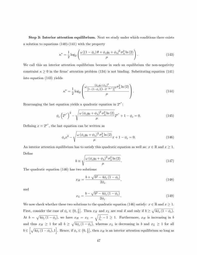
Step 3: Interior attention equilibrium. Next we study under which conditions there exists

a solution to equations (140)-(141) with the property

κ∗ =1

2log2

Ãω [(1− φc) θ + φcg0 + φλ]

2 σ2λ ln (2)

μ

!. (143)

We call this an interior attention equilibrium because in such an equilibrium the non-negativity

constraint κ ≥ 0 in the firms’ attention problem (134) is not binding. Substituting equation (141)

into equation (143) yields

κ∗ =1

2log2

⎛⎜⎝ω (φcg0+φλ)2

[1−(1−φc)(1−2−2κ∗)]

2σ2λ ln (2)

μ

⎞⎟⎠ . (144)

Rearranging the last equation yields a quadratic equation in 2κ∗:

φc

³2κ∗´2−

sω (φcg0 + φλ)

2 σ2λ ln (2)

μ2κ∗+ 1− φc = 0. (145)

Defining x ≡ 2κ∗ , the last equation can be written as

φcx2 −

sω (φcg0 + φλ)

2 σ2λ ln (2)

μx+ 1− φc = 0. (146)

An interior attention equilibrium has to satisfy this quadratic equation as well as: x ∈ R and x ≥ 1.

Define

b ≡

sω (φcg0 + φλ)

2 σ2λ ln (2)

μ. (147)

The quadratic equation (146) has two solutions:

xH =b+

pb2 − 4φc (1− φc)

2φc, (148)

and

xL =b−

pb2 − 4φc (1− φc)

2φc. (149)

We now check whether these two solutions to the quadratic equation (146) satisfy: x ∈ R and x ≥ 1.

First, consider the case of φc ∈¡0, 12

¤. Then xH and xL are real if and only if b ≥

p4φc (1− φc).

At b =p4φc (1− φc), we have xH = xL =

q1φc− 1 ≥ 1. Furthermore, xH is increasing in b

and thus xH ≥ 1 for all b ≥p4φc (1− φc), whereas xL is decreasing in b and xL ≥ 1 for all

b ∈hp4φc (1− φc), 1

i. Hence, if φc ∈

¡0, 12

¤, then xH is an interior attention equilibrium so long as

47

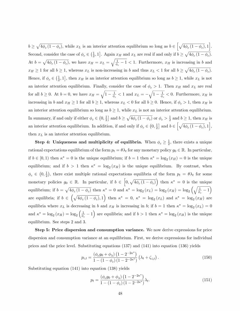
b ≥p4φc (1− φc), while xL is an interior attention equilibrium so long as b ∈

hp4φc (1− φc), 1

i.

Second, consider the case of φc ∈¡12 , 1¤. Again xH and xL are real if and only if b ≥

p4φc (1− φc).

At b =p4φc (1− φc), we have xH = xL =

q1φc− 1 < 1. Furthermore, xH is increasing in b and

xH ≥ 1 for all b ≥ 1, whereas xL is non-increasing in b and thus xL < 1 for all b ≥p4φc (1− φc).

Hence, if φc ∈¡12 , 1¤, then xH is an interior attention equilibrium so long as b ≥ 1, while xL is not

an interior attention equilibrium. Finally, consider the case of φc > 1. Then xH and xL are real

for all b ≥ 0. At b = 0, we have xH =q1− 1

φc< 1 and xL = −

q1− 1

φc< 0. Furthermore, xH is

increasing in b and xH ≥ 1 for all b ≥ 1, whereas xL < 0 for all b ≥ 0. Hence, if φc > 1, then xH is

an interior attention equilibrium so long as b ≥ 1, while xL is not an interior attention equilibrium.

In summary, if and only if either φc ∈¡0, 12

¤and b ≥

p4φc (1− φc) or φc >

12 and b ≥ 1, then xH is

an interior attention equilibrium. In addition, if and only if φc ∈¡0, 12

¤and b ∈

hp4φc (1− φc), 1

i,

then xL is an interior attention equilibrium.

Step 4: Uniqueness and multiplicity of equilibria. When φc ≥ 12 , there exists a unique

rational expectations equilibrium of the form pt = θλt for any monetary policy g0 ∈ R. In particular,

if b ∈ [0, 1) then κ∗ = 0 is the unique equilibrium; if b = 1 then κ∗ = log2 (xH) = 0 is the unique

equilibrium; and if b > 1 then κ∗ = log2 (xH) is the unique equilibrium. By contrast, when

φc ∈¡0, 12

¢, there exist multiple rational expectations equilibria of the form pt = θλt for some

monetary policies g0 ∈ R. In particular, if b ∈h0,p4φc (1− φc)

´then κ∗ = 0 is the unique

equilibrium; if b =p4φc (1− φc) then κ∗ = 0 and κ∗ = log2 (xL) = log2 (xH) = log2

³q1φc− 1´

are equilibria; if b ∈³p

4φc (1− φc), 1´then κ∗ = 0, κ∗ = log2 (xL) and κ∗ = log2 (xH) are

equilibria where xL is decreasing in b and xH is increasing in b; if b = 1 then κ∗ = log2 (xL) = 0

and κ∗ = log2 (xH) = log2

³1φc− 1´are equilibria; and if b > 1 then κ∗ = log2 (xH) is the unique

equilibrium. See steps 2 and 3.

Step 5: Price dispersion and consumption variance. We now derive expressions for price

dispersion and consumption variance at an equilibrium. First, we derive expressions for individual

prices and the price level. Substituting equations (137) and (141) into equation (136) yields

pi,t =(φcg0 + φλ)

¡1− 2−2κ∗

¢1− (1− φc) (1− 2−2κ

∗)

¡λt + ζi,t

¢. (150)

Substituting equation (141) into equation (138) yields

pt =(φcg0 + φλ)

¡1− 2−2κ∗

¢1− (1− φc) (1− 2−2κ

∗)λt. (151)

48

Second, we derive a simple expression for price dispersion at an equilibrium. Consider the case of

an equilibrium with κ∗ > 0. An equilibrium with κ∗ > 0 is an interior attention equilibrium and in

an interior attention equilibrium equation (144) holds. Equations (150) and (151) imply

Eh(pi,t − pt)

2i=

"(φcg0 + φλ)

¡1− 2−2κ∗

¢1− (1− φc) (1− 2−2κ

∗)

#2σ2ζ .

Substituting equation (144) into the last equation yields

Eh(pi,t − pt)

2i=

μω

σ2λ ln (2)22κ

∗³1− 2−2κ∗

´2σ2ζ .

Furthermore, substituting equation (137) into the last equation and rearranging yields

Eh(pi,t − pt)

2i=

μω

ln (2)

³1− 2−2κ∗

´. (152)

Next consider the case of an equilibrium with κ∗ = 0. Equation (152) holds again because in

an equilibrium with κ∗ = 0 we have Eh(pi,t − pt)

2i= 0. In summary, in any equilibrium, price

dispersion is given by equation (152). It follows that equilibrium price dispersion is an increasing

function of equilibrium attention. Third, we derive an expression for consumption variance at an

equilibrium. Substituting the monetary policy mt = g0λt and the equation for the price level (151)

into the cash-in-advance constraint (50) yields

ct =

"g0 −

(φcg0 + φλ)¡1− 2−2κ∗

¢1− (1− φc) (1− 2−2κ

∗)

#λt, (153)

implying

E£c2t¤=

"g0 −

(φcg0 + φλ)¡1− 2−2κ∗

¢1− (1− φc) (1− 2−2κ

∗)

#2σ2λ. (154)

The first term in square brackets in equation (153) equals the response of nominal spending to the

desired markup, while the second term in square brackets in equation (153) equals the response of

the price level to the desired markup. The difference between the two determines the response of

composite consumption to the desired markup.

Step 6: Optimal monetary policy has to satisfy g0 ≥ −φλφc. Having characterized the set of

rational expectations equilibria of the form pt = θλt for given monetary policy g0 and having derived

expressions for price dispersion and consumption variance, we now derive results concerning optimal

monetary policy. We begin by showing that optimal monetary policy has to satisfy g0≥ −φλφc. The

49

proof is as follows. First, at the monetary policy g0 = −φλφcwe have b = 0 and thus the unique

rational expectations equilibrium of the form pt = θλt is a zero attention equilibrium, implying that

price dispersion equals zero and consumption variance equals E£c2t¤=³φλφc

´2σ2λ. Second, consider

a monetary policy g0 < −φλφc. Price dispersion at a monetary policy g0 < −φλ

φcis weakly larger than

price dispersion at the monetary policy g0 = −φλφcbecause price dispersion is weakly larger than

zero. Furthermore, consumption variance at a monetary policy g0 < −φλφcis strictly larger than

consumption variance at the monetary policy g0 = −φλφc. This result follows from the fact that

consumption variance at an equilibrium is given by equation (154) and, for all g0 < −φλφc, we have

g0 −(φcg0 + φλ)

¡1− 2−2κ∗

¢1− (1− φc) (1− 2−2κ

∗)< −φλ

φc< 0. (155)

In summary, a monetary policy g0 < −φλφcyields weakly larger price dispersion and strictly larger

consumption variance than the monetary policy g0 = −φλφc. Hence, a monetary policy g0 < −φλ

φc

cannot be optimal. To see what this result means economically, note that the condition g0 ≥ −φλφc

can be written as φcg0 + φλ ≥ 0. Furthermore, substituting equation (141) into equation (133)

yields the following equation for the profit-maximizing price at an equilibrium

p∗i,t =φcg0 + φλ

1− (1− φc) (1− 2−2κ∗)λt. (156)

The result that optimal monetary policy has to satisfy g0 ≥ −φλφcmeans that at an optimal monetary

policy the profit-maximizing price cannot be decreasing in the desired markup, implying that

individual prices and the price level cannot be decreasing in the desired markup.

Step 7: Optimal monetary policy when φc ≥ 12 . First, when φc ≥

12 , there exists a unique

rational expectations equilibrium of the form pt = θλt for any monetary policy g0 ∈ R: if b ∈ [0, 1)

then κ∗ = 0 is the unique equilibrium; if b = 1 then κ∗ = log2 (xH) = 0 is the unique equilibrium;

and if b > 1 then κ∗ = log2 (xH) is the unique equilibrium. See step 4. Second, in the derivation

of optimal monetary policy we can focus on g0 ≥ −φλφc. See step 6. Furthermore, equation (147)

implies that the variable b is an increasing function of the monetary policy g0 for all g0 ≥ −φλφc.

Define g0 as the value of g0 ∈h−φλ

φc,∞´at which b = 1. Equation (147) implies that

g0 = −φλφc+1

φc

rμ

ωσ2λ ln (2). (157)

If g0 ∈h−φλ

φc, g0

´then b ∈ [0, 1) and κ∗ = 0 is the unique equilibrium; if g0 = g0 then b = 1 and

κ∗ = log2 (xH) = 0 is the unique equilibrium; and if g0 > g0 then b > 1 and κ∗ = log2 (xH) is the

50

unique equilibrium. Note that in the case of ωφ2λσ2λ ln(2)μ ≤ 1 we have g0 ≥ 0, whereas in the case of

ωφ2λσ2λ ln(2)μ > 1 we have g0 < 0. Hence, when ωφ2λσ

2λ ln(2)μ ≤ 1 the monetary policy g0 = 0 yields a

zero attention equilibrium, whereas when ωφ2λσ2λ ln(2)μ > 1 the central bank has to lower the money

supply after a positive markup shock to attain a zero attention equilibrium. Third, consider the

case of φc ≥ 12 and

ωφ2λσ2λ ln(2)μ ≤ 1. At the monetary policy g0 = 0, we have b ≤ 1 and therefore

κ∗ = 0 is the unique equilibrium, implying that price dispersion equals zero, Eh(pi,t − pt)

2i= 0,

and consumption variance equals zero, E£c2t¤= g20σ

2λ = 0. See equations (152) and (154). Thus, in

the case of φc ≥ 12 and

ωφ2λσ2λ ln(2)μ ≤ 1 the monetary policy g0 = 0 attains the efficient allocation.

Furthermore, any monetary policy g0 6= 0 does not attain the efficient allocation. If the equilibrium

at the monetary policy g0 6= 0 is an equilibrium with κ∗ = 0 then consumption variance is strictly

positive, while if the equilibrium at the monetary policy g0 6= 0 is an equilibrium with κ∗ > 0

then price dispersion is strictly positive. See equations (152) and (154). Hence, in the case of

φc ≥ 12 and

ωφ2λσ2λ ln(2)μ ≤ 1 the unique optimal monetary policy is g∗0 = 0. Fourth, consider the

case of φc ≥ 12 and

ωφ2λσ2λ ln(2)μ > 1. We derive optimal monetary policy in this case by showing

that the monetary policy minimizing objective (48) among all monetary policies g0 ∈h−φλ

φc, g0

iis

g0 = g0 and by showing that the monetary policy minimizing objective (48) among all monetary

policies g0 ∈ [g0,∞) is g0 = g0. Combining results then yields that in the case of φc ≥ 12 and

ωφ2λσ2λ ln(2)μ > 1 the unique optimal monetary policy among all monetary policies g0 ∈ R is g0 = g0.

For all g0 ∈h−φλ

φc, g0

i, we have b ≤ 1 and thus κ∗ = 0 is the unique equilibrium, implying

that price dispersion equals zero and consumption variance equals E£c2t¤= g20σ

2λ. Furthermore,

ωφ2λσ2λ ln(2)μ > 1 implies g0 < 0. It follows that in the case of φc ≥ 1

2 andωφ2λσ

2λ ln(2)μ > 1 the monetary

policy minimizing objective (48) among all monetary policies g0 ∈h−φλ

φc, g0

iis g0 = g0. Next, for

all g0 ∈ [g0,∞), we have b ≥ 1 and thus κ∗ = log2 (xH) is the unique equilibrium. Let us study price

dispersion. Since equilibrium price dispersion is strictly increasing in κ∗, xH is strictly increasing

in b, and b is strictly increasing in g0 for all g0 ≥ g0, it follows that price dispersion is strictly

increasing in g0 for all g0 ≥ g0. See equations (147), (148) and (152). Let us turn to consumption

variance. Equilibrium consumption is given by equation (153). Furthermore, when κ∗ = log2 (xH),

equation (144) holds. Rearranging equation (144) using g0 ≥ −φλφcyields

φcg0 + φλ1− (1− φc) (1− 2−2κ

∗)=

rμ

ωσ2λ ln (2)2κ∗. (158)

51

Substituting the last equation into equation (153) yields

ct =

∙g0 −

rμ

ωσ2λ ln (2)

³2κ∗ − 2−κ∗

´¸λt. (159)

In addition, solving equation (147) for g0 using g0 ≥ −φλφcyields

g0 = −φλφc+

b

φc

rμ

ωσ2λ ln (2). (160)

Substituting κ∗ = log2 (xH), equation (148) and equation (160) into equation (159) yields

ct =

⎡⎢⎣−φλφc+

rμ

ωσ2λ ln (2)

⎛⎜⎝ b

φc− b+

pb2 − 4φc (1− φc)

2φc+

1

b+√b2−4φc(1−φc)2φc

⎞⎟⎠⎤⎥⎦λt. (161)

Rearranging the last equation yields

ct =

"−φλφc+

rμ

ωσ2λ ln (2)

2

b+pb2 − 4φc (1− φc)

#λt. (162)

Hence, when g0 ≥ −φλφcand κ∗ = log2 (xH), equilibrium consumption is given by equation (162).

The term in square brackets in equation (162) is strictly decreasing in b for all b ≥ 1. Moreover,

in the case of φc ≥ 12 and

ωφ2λσ2λ ln(2)μ > 1, the term in square brackets in equation (162) is strictly

negative at b = 1. Thus, in the case of φc ≥ 12 and

ωφ2λσ2λ ln(2)μ > 1, consumption variance is strictly

increasing in g0 for all g0 ≥ g0. It follows that, in the case of φc ≥ 12 and

ωφ2λσ2λ ln(2)μ > 1, the

monetary policy minimizing objective (48) among all monetary policies g0 ∈ [g0,∞) is g0 = g0

because both price dispersion and consumption variance are strictly increasing in g0 for all g0 ≥ g0.

Combining results yields that in the case of φc ≥ 12 and

ωφ2λσ2λ ln(2)μ > 1 the unique optimal monetary

policy among all monetary policies g0 ∈ R is g0 = g0.

Step 8: Optimal monetary policy when φc ∈¡0, 12

¢. First, when φc ∈

¡0, 12

¢, there exist

multiple rational expectations equilibria of the form pt = θλt for some monetary policies g0 ∈ R.

We will use the following results below. If b ∈h0,p4φc (1− φc)

ithen κ∗ = 0 is an equilibrium. If

b ≥ 1 then κ∗ = log2 (xH) is an equilibrium. Furthermore, if b ∈h0,p4φc (1− φc)

´or b > 1 then

there is a unique equilibrium, whereas if b ∈hp4φc (1− φc), 1

ithen there exist multiple equilibria.

See step 4. Second, in the derivation of optimal monetary policy we can focus on g0 ≥ −φλφc. See

step 6. Furthermore, equation (147) implies that b is strictly increasing in g0 for all g0 ≥ −φλφc.

52

Define g0 as the value of g0 ∈h−φλ

φc,∞´at which b =

p4φc (1− φc). Define g0 as the value of

g0 ∈h−φλ

φc,∞´at which b = 1. Equation (147) implies that

g0 = −φλφc+

p4φc (1− φc)

φc

rμ

ωσ2λ ln (2), (163)

and

g0 = −φλφc+1

φc

rμ

ωσ2λ ln (2). (164)

For all g0 ∈h−φλ

φc, g0

´, κ∗ = 0 is the unique equilibrium. For all g0 > g0, κ∗ = log2 (xH) is the

unique equilibrium. Note that the parameter restriction ωφ2λσ2λ ln(2)μ < 4φc (1− φc) implies g0 > 0.

Third, consider the case of φc ∈¡0, 12

¢and ωφ2λσ

2λ ln(2)μ < 4φc (1− φc). At the monetary policy

g0 = 0, we have g0 < g0 and thus κ∗ = 0 is the unique equilibrium, implying that price dispersion

equals zero and consumption variance equals zero, E£c2t¤= g20σ

2λ = 0. See equations (152) and

(154). Thus, when φc ∈¡0, 12

¢and ωφ2λσ

2λ ln(2)μ < 4φc (1− φc) the monetary policy g0 = 0 attains

the efficient allocation as the unique equilibrium allocation. Moreover, any monetary policy g0 6= 0

does not attain the efficient allocation. If the equilibrium at the monetary policy g0 6= 0 is an

equilibrium with κ∗ = 0 then consumption variance is strictly positive, while if the equilibrium

at the monetary policy g0 6= 0 is an equilibrium with κ∗ > 0 then price dispersion is strictly

positive. See equations (152) and (154). Hence, when φc ∈¡0, 12

¢and ωφ2λσ

2λ ln(2)μ < 4φc (1− φc)

the unique optimal monetary policy is g∗0 = 0. Fourth, consider the case of φc ∈¡0, 12

¢and

ωφ2λσ2λ ln(2)μ ≥ 4φc (1− φc). For all monetary policies g0 ∈

h−φλ

φc, g0

i, κ∗ = 0 is an equilibrium. Let

us rank these zero attention equilibria for different monetary policies g0 ∈h−φλ

φc, g0

i. In a zero

attention equilibrium price dispersion equals zero and consumption variance equals E£c2t¤= g20σ

2λ.

The parameter restriction ωφ2λσ2λ ln(2)μ ≥ 4φc (1− φc) implies g0 ≤ 0. Hence, in the case of φc ∈

¡0, 12

¢and ωφ2λσ

2λ ln(2)μ ≥ 4φc (1− φc), the value of objective (48) at an equilibrium with κ∗ = 0 is strictly

decreasing in g0 for all g0 ∈h−φλ

φc, g0

i. Next, for all monetary policies g0 ≥ g0, κ∗ = log2 (xH)

is an equilibrium. Let us rank these equilibria with κ∗ = log2 (xH) for different monetary policies

g0 ≥ g0. It follows from equations (152), (147) and (148) that price dispersion at an equilibrium

with κ∗ = log2 (xH) is strictly increasing in g0 for all g0 ≥ g0. Furthermore, the same derivation as

in step 7 yields that when g0 ≥ −φλφcand κ∗ = log2 (xH) equilibrium consumption equals

ct =

"−φλφc+

rμ

ωσ2λ ln (2)

2

b+pb2 − 4φc (1− φc)

#λt. (165)

53

The term in square brackets in equation (165) is strictly decreasing in b for all b ≥ 1. Moreover,

in the case of φc ∈¡0, 12

¢and ωφ2λσ

2λ ln(2)μ ≥ 4φc (1− φc), the term in square brackets in equation

(165) is strictly negative at b = 1. Hence, in the case of φc ∈¡0, 12

¢and ωφ2λσ

2λ ln(2)μ ≥ 4φc (1− φc),

both price dispersion and consumption variance at an equilibrium with κ∗ = log2 (xH) are strictly

increasing in g0 for all g0 ≥ g0, implying that the value of objective (48) at an equilibrium with

κ∗ = log2 (xH) is strictly increasing in g0 for all g0 ≥ g0. Finally, in the case of φc ∈¡0, 12

¢and

ωφ2λσ2λ ln(2)μ ≥ 4φc (1− φc), let us compare the zero attention equilibrium at g0 = g0 to the equilibrium

with κ∗ = log2 (xH) at g0 = g0. At g0 = g0 we have b = 1 and thus log2 (xH) = log2³1φc− 1´> 0

in the case of φc ∈¡0, 12

¢. See equation (148). It follows from equation (152) that price dispersion

is strictly smaller in a zero attention equilibrium than in the equilibrium with κ∗ = log2 (xH) at

g0 = g0. In addition, consumption variance is strictly smaller in the zero attention equilibrium at

g0 = g0 than in the equilibrium with κ∗ = log2 (xH) at g0 = g0 because the parameter restrictions

φc ∈¡0, 12

¢and ωφ2λσ

2λ ln(2)μ ≥ 4φc (1− φc) imply"

−φλφc+

p4φc (1− φc)

φc

rμ

ωσ2λ ln (2)

#2σ2λ <

⎡⎣−φλφc+

rμ

ωσ2λ ln (2)

2

1 +q(1− 2φc)2

⎤⎦2 σ2λ.Hence, in the case of φc ∈

¡0, 12

¢and ωφ2λσ

2λ ln(2)μ ≥ 4φc (1− φc), the zero attention equilibrium at

g0 = g0 yields a strictly smaller value of objective (48) than the equilibrium with κ∗ = log2 (xH)

at g0 = g0. In summary, in the case of φc ∈¡0, 12

¢and ωφ2λσ

2λ ln(2)μ ≥ 4φc (1− φc), we have the

following four results: (i) there is a unique rational expectations equilibrium of the form pt = θλt

for all g0 ∈h−φλ

φc, g0

´and g0 > g0, whereas there are multiple rational expectations equilibria of

the form pt = θλt for all g0 ∈ [g0, g0], (ii) the value of objective (48) at an equilibrium with κ∗ = 0 is

strictly decreasing and continuous in g0 for all g0 ∈h−φλ

φc, g0

i, (iii) the value of objective (48) at an

equilibrium with κ∗ = log2 (xH) is strictly increasing in g0 for all g0 ≥ g0, and (iv) the zero attention

equilibrium at g0 = g0 yields a strictly smaller value of objective (48) than the equilibrium with

κ∗ = log2 (xH) at g0 = g0. It follows that, in the case of φc ∈¡0, 12

¢and ωφ2λσ

2λ ln(2)μ ≥ 4φc (1− φc),

the best the central bank can do among all monetary policies g0 ∈ R if the central bank wants to

obtain a unique equilibrium of the form pt = θλt is to choose a g0 marginally below g0.

54

References

[1] Adam, Klaus (2007). “Optimal Monetary Policy with Imperfect Common Knowledge,” Journal

of Monetary Economics, 54(2), 267-301.

[2] Angeletos, George-Marios, and Jennifer La’O (2008). “Dispersed Information over the Business

Cycle: Optimal Fiscal and Monetary Policy,” Discussion paper, MIT.

[3] Angeletos, George-Marios, and Alessandro Pavan (2007). “Efficient Use of Information and

Social Value of Information,” Econometrica, 75(4), 1103-1142.

[4] Angeletos, George-Marios, and Alessandro Pavan (2009). “Policy with Dispersed Information,”

Journal of the European Economic Association, 7(1), 11—60.

[5] Baeriswyl, Romain, and Camille Cornand (2010). “The Signaling Role of Policy Action,”

Journal of Monetary Economics, 57(6), 682-695.

[6] Ball, Laurence, N. Gregory Mankiw, and Ricardo Reis (2005). “Monetary Policy for Inattentive

Economies,” Journal of Monetary Economics, 52(4), 703-725.

[7] Boivin, Jean, Marc Giannoni, and Ilian Mihov (2009). “Sticky Prices and Monetary Policy:

Evidence from Disaggregated U.S. Data,” American Economic Review, 99(1), 350-384.

[8] Christiano, Lawrence J., Martin Eichenbaum, and Charles L. Evans (1999). “Monetary Policy

Shocks: What Have We Learned and to What End?” In Handbook of Macroeconomics, edited

by John B. Taylor and Michael Woodford, New York: Elsevier.

[9] Giannoni, Marc, and Michael Woodford (2010). “Optimal Target Criteria for Stabilization

Policy,” Discussion paper, Columbia University.

[10] Hellwig, Christian (2005). “Heterogeneous Information and the Welfare Effects of Public In-

formation Disclosures,” Discussion paper, UCLA.

[11] Hellwig, Christian, and Laura Veldkamp (2009). “Knowing What Others Know: Coordination

Motives in Information Acquisition,” Review of Economic Studies, 76(1), 223-251.

[12] Leeper, Eric M., Christopher A. Sims, and Tao Zha (1996). “What Does Monetary Policy

Do?” Brookings Papers on Economic Activity, 1996(2), 1-63.

55

[13] Lorenzoni, Guido (2010). “Optimal Monetary Policy with Uncertain Fundamentals and Dis-

persed Information,” Review of Economic Studies, 77(1), 305-338.

[14] Mackowiak, Bartosz, Emanuel Moench, and Mirko Wiederholt (2009). “Sectoral Price Data

and Models of Price Setting,” Journal of Monetary Economics, 56(S), 78-99.

[15] Mackowiak, Bartosz, and Mirko Wiederholt (2009). “Optimal Sticky Prices under Rational

Inattention,” American Economic Review, 99(3), 769-803.

[16] Mackowiak, Bartosz, and Mirko Wiederholt (2010). “Business Cycle Dynamics under Rational

Inattention,” Discussion paper, ECB and Northwestern University.

[17] Mankiw, N. Gregory, and Ricardo Reis (2002). “Sticky Information versus Sticky Prices: A

Proposal to Replace the New Keynesian Phillips Curve,” Quarterly Journal of Economics,

117(4), 1295-1328.

[18] Mondria, Jordi (2010). “Portfolio Choice, Attention Allocation, and Price Comovement,” Jour-

nal of Economic Theory, forthcoming.

[19] Morris, Stephen, and Hyun Song Shin (2002). “Social Value of Public Information,” American

Economic Review, 92(5), 1521-1534.

[20] Nakamura, Emi, and Jón Steinsson (2008). “Five Facts about Prices: A Reevaluation of Menu

Cost Models,” Quarterly Journal of Economics, 123(4), 1415-1464.

[21] Paciello, Luigi (2009). “Monetary Policy Activism and Price Responsiveness to Aggregate

Shocks under Rational Inattention,” Discussion paper, Einaudi Institute for Economics and

Finance.

[22] Rao, C. R. (1973). Linear Statistical Inference and its Applications, New York: Wiley.

[23] Sims, Christopher A. (2003). “Implications of Rational Inattention,” Journal of Monetary

Economics, 50(3), 665-690.

[24] Smets, Frank, and Rafael Wouters (2007). “Shocks and Frictions in U.S. Business Cycles: A

Bayesian DSGE Approach,” American Economic Review, 97(3), 586-606.

56

[25] Svensson, Lars E. O., and Michael Woodford (2003). “Indicator Variables for Optimal Policy,”

Journal of Monetary Economics, 50(3), 691-720.

[26] Svensson, Lars E. O., and Michael Woodford (2004). “Indicator Variables for Optimal Policy

under Asymmetric Information,” Journal of Economic Dynamics and Control, 28(4), 661-690.

[27] Uhlig, Harald (2005). “What Are the Effects of Monetary Policy on Output? Results from an

Agnostic Identification Procedure,” Journal of Monetary Economics, 52, 381-419.

[28] Woodford, Michael (2002). “Imperfect Common Knowledge and the Effects of Monetary Pol-

icy,” In Knowledge, Information, and Expectations in Modern Macroeconomics: In Honor of

Edmund S. Phelps, ed. Philippe Aghion et al. Princeton and Oxford: Princeton University

Press.

[29] Woodford, Michael (2003). Interest and Prices. Foundations of a Theory of Monetary Policy.

Princeton and Oxford: Princeton University Press.

[30] Woodford, Michael (2009). “Information-Constrained State-Dependent Pricing,” Journal of

Monetary Economics, 56(S), 100-124.

57

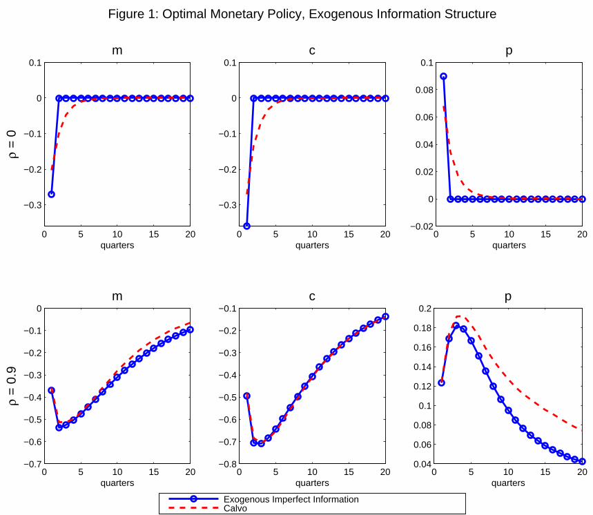
0 5 10 15 20

−0.3

−0.2

−0.1

0

0.1m

ρ =

0

quarters0 5 10 15 20

−0.3

−0.2

−0.1

0

0.1c

quarters0 5 10 15 20

−0.02

0

0.02

0.04

0.06

0.08

0.1p

quarters

0 5 10 15 20−0.7

−0.6

−0.5

−0.4

−0.3

−0.2

−0.1

0m

ρ =

0.9

quarters0 5 10 15 20

−0.8

−0.7

−0.6

−0.5

−0.4

−0.3

−0.2

−0.1c

quarters

Exogenous Imperfect InformationCalvo

Figure 1: Optimal Monetary Policy, Exogenous Information Structure

0 5 10 15 200.04

0.06

0.08

0.1

0.12

0.14

0.16

0.18

0.2p

quarters

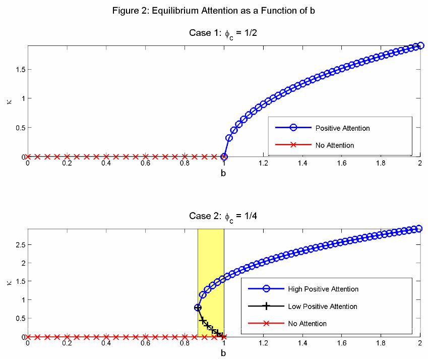
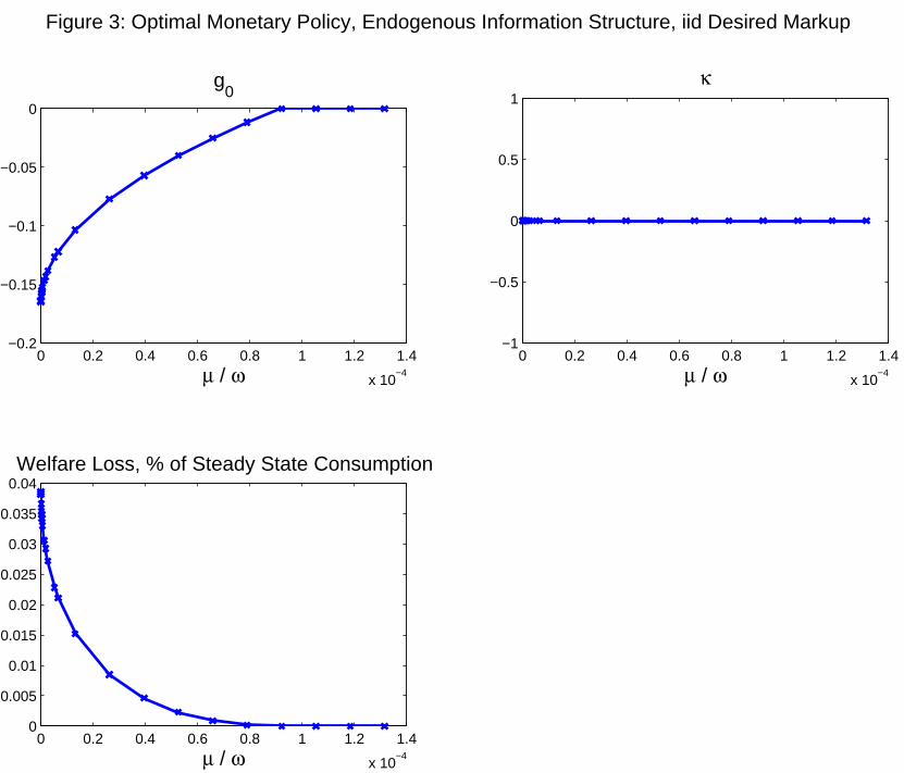
0 0.2 0.4 0.6 0.8 1 1.2 1.4

x 10−4

−0.2

−0.15

−0.1

−0.05

0

g0

μ / ω0 0.2 0.4 0.6 0.8 1 1.2 1.4

x 10−4

−1

−0.5

0

0.5

1κ

μ / ω

Figure 3: Optimal Monetary Policy, Endogenous Information Structure, iid Desired Markup

0 0.2 0.4 0.6 0.8 1 1.2 1.4

x 10−4

0

0.005

0.01

0.015

0.02

0.025

0.03

0.035

0.04Welfare Loss, % of Steady State Consumption

μ / ω

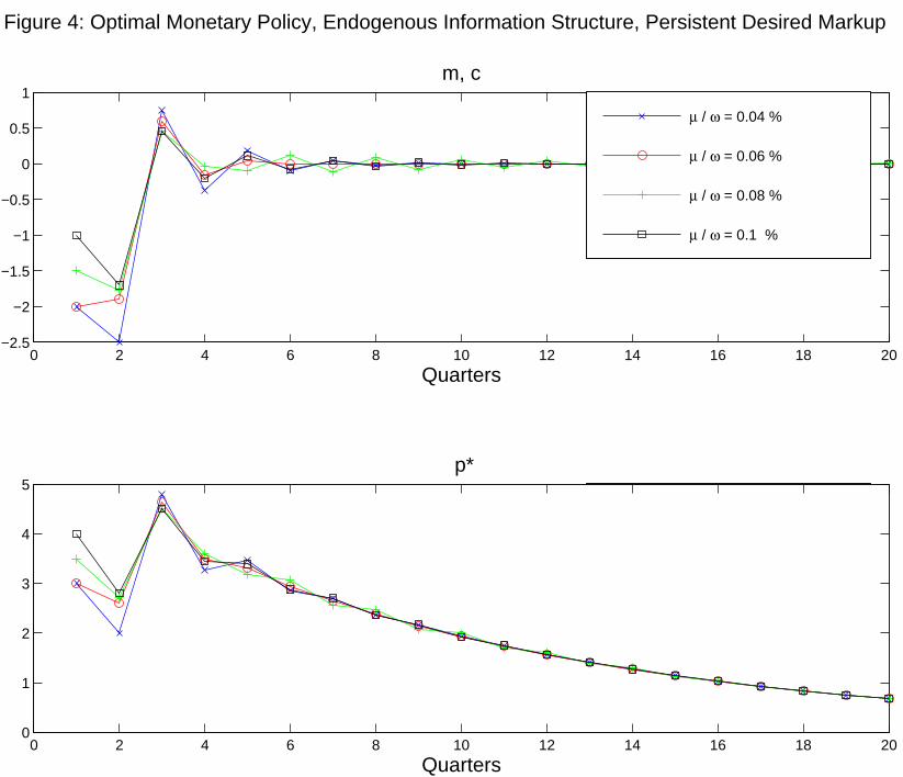
0 2 4 6 8 10 12 14 16 18 20−2.5

−2

−1.5

−1

−0.5

0

0.5

1m, c

Quarters

μ / ω = 0.04 %

μ / ω = 0.06 %

μ / ω = 0.08 %

μ / ω = 0.1 %

μ / ω = 0.04 %

μ / ω = 0.06 %

μ / ω = 0.08 %

μ / ω = 0.1 %

Figure 4: Optimal Monetary Policy, Endogenous Information Structure, Persistent Desired Markup

0 2 4 6 8 10 12 14 16 18 200

1

2

3

4

5 p*

Quarters

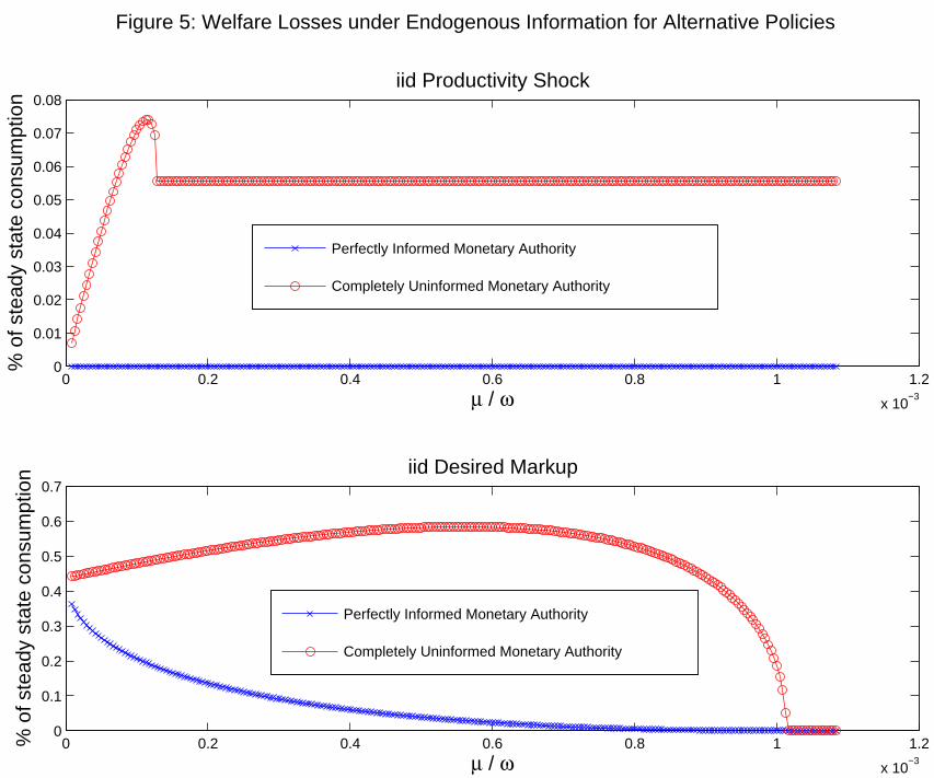
0 0.2 0.4 0.6 0.8 1 1.2

x 10−3

0

0.1

0.2

0.3

0.4

0.5

0.6

0.7iid Desired Markup

μ / ω

% o

f ste

ady

stat

e co

nsum

ptio

nFigure 5: Welfare Losses under Endogenous Information for Alternative Policies

0 0.2 0.4 0.6 0.8 1 1.2

x 10−3

0

0.01

0.02

0.03

0.04

0.05

0.06

0.07

0.08iid Productivity Shock

μ / ω

% o

f ste

ady

stat

e co

nsum

ptio

n

Perfectly Informed Monetary Authority

Completely Uninformed Monetary Authority

Perfectly Informed Monetary Authority

Completely Uninformed Monetary Authority