Embed Size (px)
Citation preview

1
Exogenous Targeting Instruments under Differing Information Conditions.
September 10, 2003
John Spraggon Department of Economics
Lakehead University 955 Oliver Rd.
Thunder Bay, ON P7B 5E1
Abstract This paper tests the ability of an exogenous targeting instrument to induce compliance when the regulator cannot observe the emissions of the individual polluters. Spraggon (2002 and 2001a) shows that although these instruments are able to induce groups to the target outcome they are not able to induce individuals to make the socially optimal decision. This study investigates whether the information individuals have about others payoffs effects how they make their decisions in this environment. Ledyard (1995) suggests that when subjects have less information in public goods experiments they are more likely to choose the Nash equilibrium decision. In the exogenous targeting instrument environment the Nash equilibrium decision is also the socially optimal decision. Thus, if this result carries over, subjects will be more likely choose the socially optimal decision. Keywords: Moral Hazard in Groups, Exogenous Targeting Instruments, Experiments, Information (JEL C72, C92, D70). Acknowledgements: This research is sponsored through a grant from the Senate Research Committee at Lakehead University. Please do not quote without permission, any comments would be appreciated.

2
Introduction
Moral hazard in groups is a common social dilemma applicable in a wide range of
settings. Workers choosing effort levels, polluters choosing emission levels are two
primary examples. Moral hazard in groups is characterized by a principal who would
like to induce an agent to make a specific choice which is not in the agent’s best interest,
and the agent’s action is unobservable to the principal. Many authors discuss and
provide refinement to the use of “Exogenous Targeting Instruments” as a theoretical
solution to the moral hazard in groups problem (for example Holmstrom 1982, McAfee
and McMilan 1991, Segerson 1988 and Xepapadeas 1992, 1995). This paper is one in a
series that uses controlled laboratory experiments to provide some empirical evidence as
to the efficacy of these instruments. Recent papers by authors such as Cochard et al.
(2002), Spraggon (2002, 2000a) and Vossler et al. (2002) suggests that exogenous
targeting instruments are able to induce groups of individuals to comply with a standard
under a number of different circumstances, including when subjects have heterogeneous
payoff functions (Spraggon 2002a) and when subjects are also involved in a market
(Vossler et al. 2002).1 However, these instruments are typically unable to induce
individuals to choose the socially optimal decision on average. The purpose of this
experiment is to determine whether the information individuals have influences whether
or not their decisions correspond with theoretical predictions.
Clearly there are many different situations that involve moral harzard in groups.
In terms of the worker effort problem, some work groups may have excellent information
about the cost of effort of co-workers (sports teams, production shop floors) while some
1 Nalbantian and Schotter (1997) investigate a different exogenous targeting instrument which is unable to induce the group to the target outcome.

3
may not (management may not have a good idea of the cost of effort for production floor
workers and vice versa). Similarly, some non-point source pollution problems may
involve very similar polluters with excellent information about each other i.e. dairy
farmers. Other situations may involve many different types of polluters (agricultural,
industrial and municipal) who may not have good information about each other. Horan
(2001) lists ten different non-point source pollution sites. Of these at least two involve
different types of sources, and two (one of these and one which does not involve different
types of sources) cross state lines.2
The experiment involves two treatment variables: the information condition (full,
partial or no information), and the payoff functions (homogeneous or heterogeneous).
Under the full information condition subjects know the number of people in their group
and everyone's payoff function. This is the information condition under which Spraggon
(2002, and 2000a) were conducted. Under the partial information condition subjects
know the number of people in their group but have no information about the payoff
functions of the other people. Under the no information condition subjects only know
their own payoff function and have no information about the number of people in their
group or the payoff functions of the others in their group. This is similar to the
information treatment for public goods experiments investigated in Marks and Croson
(1999).3 Although there were no significant effects of information at the aggregate level,
they observed a greater degree of convergence to the Nash Equilibrium in their
incomplete information case than in their full or partial information case. Rondeau et al.
2 Specifically, Chesapeak Bay involves both agricultural and urban sources and Dillon Creek involves urban, septic and ski areas. 3 In Marks and Croson’s partial information condition subjects knew the sum of the groups valuation for the public good.

4
(1999) investigate information in a one-shot provision point with money back guarantee,
a proportional rebate and heterogeneous agents with large groups (N=45). They also find
no significant effects. As a result, I conjecture that under the no information condition
subjects will be more likely to choose the socially optimal decision over time. However,
it may be the case that subjects find the treatments in which they have less information
more difficult and as a result may be more likely to choose their decision number
randomly.
A secondary purpose of this paper is to investigate the hypothesis that subjects
use simple heuristic to make their decisions. Spraggon (2000b) discusses individual
decision making in the previous exogenous targeting instrument experiments. They show
that individual decision making is best described by a simple heuristic where subjects
choose the target divided by the number of people in the group in early periods. As a
result, reducing the amount of information that subjects have about the number of people
in their group, removes this heuristic as a possible solution strategy and may make the
decision process more difficult for the subjects. A censored form of Anderson, Goeree
and Holt’s (1998) quantal response model is used to differentiate between decision error
and preference explanations as to why subject’s decisions differ from the dominant
strategy Nash decision. By estimating the error in the decision making process we are
able to determine whether or not subjects found the environment more difficults.
The results are consistent with the results of previous experiments (Ledyrad 1995,
and Marks and Croson 1999) in that different information conditions have different
effects on groups where the subjects have homogenous or heterogeneous payoff
functions. The differences here seem to be due to homogenous subjects playing more

5
randomly when they know the number of people in the group but not their payoff
functions, and more risk-aversely when they have no information, whereas heterogeneous
subjects play more randomly when they have no information, and more risk-aversely
when they know the number of people in their group. Moreover, we observe
convergence to the Nash prediction for homogeneous groups under partial and full
information and convergence for the heterogeneous groups under no and partial
information.
The Moral Hazard in Groups Experiment
The design of the experiment is based on a standard model of non-point source
pollution used by authors such as Segerson (1988), Malik (1990) and Xepapadeas (1995)
and reported in Spraggon (2002).4 Subjects take the role of firms whose decisions, for
simplicity, correspond to the level of emissions. The larger the decision number the more
emissions that the firm releases and the higher the subject’s payoff up to some maximum
decision number which corresponds to the firms uncontrolled level of emission. This part
of the subject’s payoff is described as their private payoff and is provided to the subjects
in a table. It can be described by the following function:
2max )(004.025)( nnnn xxxB −−= (1)
where Bn is the benefit function, xn is the decision number, xnmax is the maximum
decision number and n indexes the individual subjects (n=1..6). This functional form and
the parameters where chosen for mathematical convenience.
4 Nalbantian and Schotter’s (1997) experiment was also used as a model specifically for the number of subjects per group and number of periods per session. This experiment differs from Nalbantian and Schotter’s in terms of being framed as a public bad rather than a public good. See Park (2001) for a comparison of these frameworks.

6
The primary research question is whether the instruments suggested by Segerson
(1988) are able to induce firms to reduce their emissions to the socially optimal outcome.
We look at one specific form of the instrument suggested by Segerson: The tax/subsidy
instrument taxes or provides a subsidy to everyone in the group depending on the
difference between the target aggregate group decision number (which I refer to as the
group total) and the actual group total. This instrument is a linear function of the
difference between the actual and the target group totals. To ensure that subjects were
clear that this group payoff could be positive or negative it was presented as:
<−≥−
=150)150(3.0150)150(3.0
)(XifXXifX
XT (2)
where T(X) is the group benefit function, X is the aggregate decision number (or group
total ∑ ==
6
1n nxX ), 150 is the target and 0.3 is the tax and subsidy rate. As a result each
subject faces the following payoff function:
)150(3.0)(004.025 6
12max −−−−=Π ∑ =n nnnn xxx . (3)
This payoff function has a unique maximum which can be found by differentiating Πn
with respect to xn, leading to the solution: 75max* −= nn xx . Thus, the payoff maximizing
decision is for each subject to reduce their decision number from the maximum by
seventy-five. There are three different subject types. For the homogeneous sessions all
six of the subjects are medium capacity: xnmax= 100, xn
*= 25, for the heterogeneous
sessions three of the six subjects are large capacity: xnmax= 125, xn
*= 50 and three small
capacity subjects: xnmax= 75, xn
*= 0. There is also a group optimal solution under this
instrument. If all subjects choose zero the payoff of the group is maximized. This is not

7
a Nash equilibrium as it is in each individual’s best interest to reduce their decision
number from the maximum by seventy-five.
Clearly subjects may not necessarily behave as payoff maximizers. There are
many studies including (Spraggon 2001b, Anderson, Goeree and Holt 1998) which
discuss this issue. The censored form of Anderson, Goeree and Holt’s (1998) quantal
response model will be used to estimate the importance of decision error and preference
explanations for any deviations from payoff maximizing behavior.
The level of information that the subjects have about the number and payoffs of
other people in the group is the treatment variable of interest in this paper. We
investigate three different cases: Full Information, Partial Information and No
Information. In all three cases subjects know their own payoff functions. Under the full
information condition subjects know the number of other subjects in their group as well
as the payoffs of the others in their group. Under the Partial Information condition
subjects know how many people are in their group but do not have information about the
payoffs of the others in their group. Under the No Information condition subjects do not
know either the number of people in their group or the payoffs of the others in their
group.
This experiment is concerned with data from two separate sources. Data for the
full information treatment was collected at McMaster University and the data for the
partial and no information treatments were collected at Lakehead University. A previous
set of experiments has been conducted at both of these sites in order to ensure
consistency between the results (Moir and Spraggon 2002). Moreover, the procedures
used to conduct the sessions were identical except for the information provided to the

8
subjects (the treatment variable) and the fact that a session at McMaster consisted of one
group of six subjects while a session at Lakehead consisted of two groups of six subjects.
This was done so that if subjects just assume that the other people in the room comprised
their group in the no information conditions the simple heuristic decision would not be
the Nash equilibrium.
Theoretical Predictions The primary questions addressed by this study concern the average level of
aggregate decision number (group total). The purpose of these exogenous targeting
instruments is to reduce the ambient level of pollution to the target level. As a result, the
first hypothesis concerns the ability of this instrument to reduce the group total to the
target level for each of the treatments. A secondary concern is whether this instrument is
able to induce individuals to reduce their emissions to the optimal level.
Hypothesis 1: The Tax/Subsidy Instrument will be able to induce the group to the target outcome independent of the information condition. The Tax/Subsidy instrument induces the optimal decision as a dominant strategy
regardless of the information that subjects have. Indeed the less information they have
about other subjects the more likely they should be to concentrate on their own payoff
function. Moreover, the Tax/Subsidy instrument is designed such that the larger the
deviation from the target outcome the larger the fine and as a result the more likely that
subjects will go bankrupt and be removed from the group.
Hypothesis 2: Less information will result in subjects decisions being closer to the Nash decision. This hypothesis comes from the results of the Marks and Croson (1999) study.
As discussed in the introduction they found that although on average there was no

9
difference across the information conditions they did find greater convergence to the
Nash equilibrium in the treatments with less information. If this result transfers over into
this environment we should observe similar convergence to both the target at the
aggregate level and the Nash decision numbers at the individual level.
Mark’s and Croson’s (1999) study suggested that in public goods environments
when information was removed decisions converged more closely to the Nash
equilibrium. There are two reasons why decisions may diverge from the Nash
equilibrium. The first is that subject’s decisions have a random component to them due
to some explanation such as error. The second is that preferences are such that subjects
are maximizing something other than their simple monetary payoff. Therefore, when
information is removed either the experimental environment becomes simpler and so the
amount of error is reduced or the reduction in information changes the subjects
preferences (for example if you do not know that your contributions will benefit 10 other
people you may not receive as much utility through altruism as if you did have this
information).5 The Tobit model allows us to estimate both the level of error as well as
the preference maximizing decision number.6 This will allow us to differentiate between
differences, which are due to error and differences that are due to preferences.
Results The results are separated into a number of different sections. The first two results
deal with the aggregate decision numbers. First the session means are discussed and then
the convergence properties are investigated. Then we look at the mean, Tobit estimates
5 See Goeree et al. (2002) for a detailed discussion of altruism. 6 Greene (2000) and StataCorp (2001) were used as guides for the econometrics with time-series of cross-section data.

10
and convergence of the individual decision numbers. Finally, the implications of the
number of subjects who went bankrupt under each treatment are discussed.
Result 1: Information has no effect on the aggregate decision number The first question is, are there significant differences at the aggregate level between the
different information conditions. Table 1 suggests that there are differences but Analysis
of Variance (Table 2) suggests that they are not significant.7 This is consistent with the
results for information found by previous experiments (Marks and Croson 1999).
Table 1: Mean Group Total by Treatment
Information No Info Partial Info Full Info Total
Heterogeneous 196.63 12.19
3
174.69 23.03
3
170.47 6.62
3
180.60* 8.76
9
Homogeneous 150.80 7.78
3
174.51 17.65
3
158.44 7.70
3
161.25 6.94
9
Total 173.71 12.12
6
174.60 12.98
6
164.45 5.28
6
170.92* 5.91 18
Each cell contains mean, standard error and frequency. An * indicates that the Group Total is significantly different from 150 and the 5% level. Table 2: Analysis of Variance, Mean Group Total Number of obs =18 R-squared = 0.3510 Root MSE =24.02 Adj R-squared = 0.0806 Source Partial SS Df MS F Prob >F Model 3746.12 5 749.22 1.30 0.3277 Information 378.98 2 189.49 0.33 0.7264 Homogeneity 1684.32 1 1684.32 2.92 0.1133 Info*Hom 1682.82 2 841.41 1.46 0.27 Residual 6926.17 12 577.18 Total 10672.29 17 627.78
7 These results are unchanged if we look at medians (see Appendix Tables 1 and 2).

11
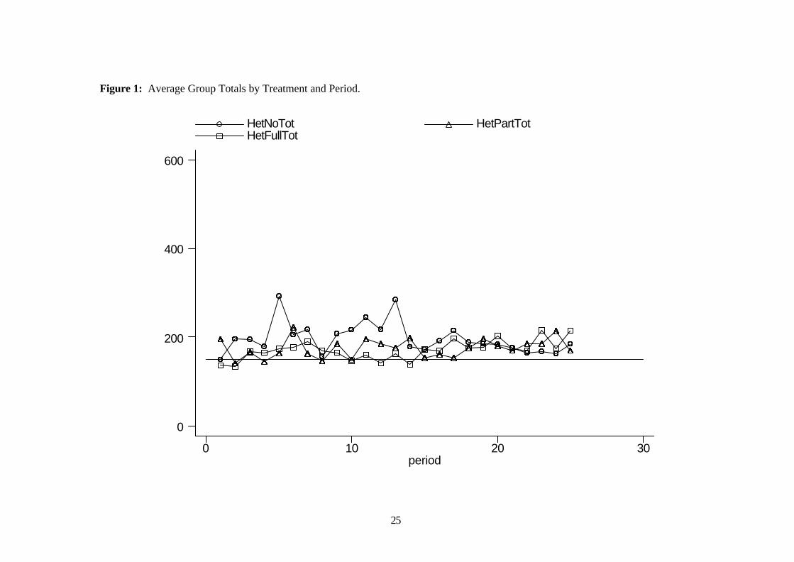
Figures 1 and 2 show the average group totals over the three sessions in each cell. Notice
that both for heterogeneous (Figure 1) and homogeneous (Figure 2) groups there is not
much difference between the lines representing the average group total in any of the
periods.
This suggests that the information that polluters have about the other participants
under the tax/subsidy instrument will not have any significant effects on the ability of this
instrument to reduce the aggregate decision number to the target.
Result 2: There are significant reductions in efficiencies due to both Heterogeneity and Information. Efficiency is defined as the change in the value of the social planner’s problem as
a percentage of the optimal change in the social planner’s problem. In this experiment
the social planner’s problem is to maximize the producer’s payoffs minus the social cost
of pollution:
)(3.0)(004.025max 6
1
6
12max ∑∑ ==−−−=
n nn nn xxxSP . (4)
Efficiency is then given by:
StatusQuoOptimal
StatusQuoActual
SPSPSPSP
E−
−= (5)
where SPActual is the actual value of the social planner’s problem given the choices of the
subjects, SPStatusQuo is the value of the social planner’s problem if all of the subjects
choose their maximum decision (xnmax) and SPOptimal is the value of the social planner’s
problem if all of the subjects choose their optimal decision (xn*). The value of efficiency
ranges between 0 and 1 and is represented in Table 3 as a percentage. Notice that there
are real differences in efficiency across the treatments. The heterogeneous groups have
lower efficiencies and No and Partial Information sessions have lower efficiencies than
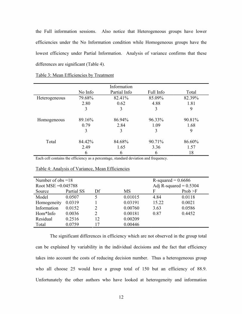
12
the Full information sessions. Also notice that Heterogeneous groups have lower
efficiencies under the No Information condition while Homogeneous groups have the
lowest efficiency under Partial Information. Analysis of variance confirms that these
differences are significant (Table 4).
Table 3: Mean Efficiencies by Treatment
Information No Info Partial Info Full Info Total
Heterogeneous 79.68% 2.80
3
82.41% 0.62
3
85.09% 4.88
3
82.39% 1.81
9
Homogeneous 89.16% 0.79
3
86.94% 2.84
3
96.33% 1.09
3
90.81% 1.68
9
Total 84.42% 2.49
6
84.68% 1.65
6
90.71% 3.36
6
86.60% 1.57 18
Each cell contains the efficiency as a percentage, standard deviation and frequency. Table 4: Analysis of Variance, Mean Efficiencies Number of obs =18 R-squared = 0.6686 Root MSE =0.045788 Adj R-squared = 0.5304 Source Partial SS Df MS F Prob >F Model 0.0507 5 0.01015 4.84 0.0118 Homogeneity 0.0319 1 0.03191 15.22 0.0021 Information 0.0152 2 0.00760 3.63 0.0586 Hom*Info 0.0036 2 0.00181 0.87 0.4452 Residual 0.2516 12 0.00209 Total 0.0759 17 0.00446
The significant differences in efficiency which are not observed in the group total
can be explained by variability in the individual decisions and the fact that efficiency
takes into account the costs of reducing decision number. Thus a heterogeneous group
who all choose 25 would have a group total of 150 but an efficiency of 88.9.
Unfortunately the other authors who have looked at heterogeneity and information

13
(Marks and Croson 1999 and Rondeau et al. 1999) look at the results with respect to
efficiency. Clearly both heterogeneity and reductions in information complicate the
environment and reduce efficiency. Moreover, we observe different effects of
information on groups with homogeneous and heterogeneous payoff functions as
observed for public goods (Ledyard 1995).
Result 3: Greater convergence is observed for the No Information case with Heterogeneous payoff functions and the Partial Information case with Homogeneous payoff functions. Marks and Croson (1999) use a random effects regression with period and period
squared to show greater convergence to the Nash outcome for their aggregate data. We
estimate this model (Table 5), an asymptotic convergence model suggested by Noussair
et al. (1995) (Table 6) and a combination of the two models (Table 7).
Table 5 Marks and Croson Convergence model
Heterogeneous Homogeneous No Info Partial
Info Full Info No Info Partial
Info Full Info
Observations Prob > X2*
75 0.0222
75 0.6126
75 0.0337
75 0.2112
75 0.1994
75 0.6712
Constant 178.28 (20.96) 0.000
168.84 (25.99) 0.000
157.01 (16.07) 0.000
145.91 (20.76) 0.000
150.88 (20.62) 0.000
168.21 (13.36) 0.000
Period 6.54 (3.43) 0.057
-0.143 (3.34) 0.966
-0.287 (2.82) 0.919
-1.55 (3.68) 0.673
4.96 (2.75) 0.071
-1.96 (2.19) 0.371
Period2 -0.302 (0.128) 0.019
0.0349 (0.125) 0.779
0.0778 (0.105) 0.460
0.113 (0.137) 0.409
-0.185 (0.103) 0.072
0.071 (0.082) 0.384
X2: ui=0 0.073 0.000 0.401 1.000 0.0000 0.078 Group Totalit = α + β1ti + β2ti
2 + + ui + Єit. Each cell contains the estimated coefficient, standard error and p-value. The Noussair et al. asymptotic model uses the inverse of period to estimate the
asymptotic starting value and (period-1)/period to estimate the asymptotic ending value.
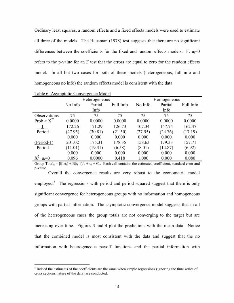
14
Ordinary least squares, a random effects and a fixed effects models were used to estimate
all three of the models. The Hausman (1978) test suggests that there are no significant
differences between the coefficients for the fixed and random effects models. F: ui=0
refers to the p-value for an F test that the errors are equal to zero for the random effects
model. In all but two cases for both of these models (heterogeneous, full info and
homogeneous no info) the random effects model is consistent with the data
Table 6: Asymptotic Convergence Model Heterogeneous Homogeneous No Info Partial
Info Full Info No Info Partial
Info Full Info
Observations Prob > X2*
75 0.0000
75 0.0000
75 0.0000
75 0.0000
75 0.0000
75 0.0000
__1__ Period
172.26 (27.95) 0.000
171.29 (30.81) 0.000
126.73 (21.50) 0.000
107.34 (27.55) 0.000
147.74 (24.76) 0.000
162.47 (17.19) 0.000
(Period-1) Period
201.02 (11.01) 0.000
175.31 (19.31) 0.000
178.35 (6.58) 0.000
158.63 (8.01) 0.000
179.33 (14.87) 0.000
157.71 (6.92) 0.000
X2: ui=0 0.096 0.0000 0.418 1.000 0.000 0.080 Group Totalit = β(1/ti) + B(ti-1)/ti + ui + Єit. Each cell contains the estimated coefficient, standard error and p-value. Overall the convergence results are very robust to the econometric model
employed.8 The regressions with period and period squared suggest that there is only
significant convergence for heterogeneous groups with no information and homogeneous
groups with partial information. The asymptotic convergence model suggests that in all
of the heterogeneous cases the group totals are not converging to the target but are
increasing over time. Figures 3 and 4 plot the predictions with the mean data. Notice
that the combined model is most consistent with the data and suggest that the no
information with heterogeneous payoff functions and the partial information with
8 Indeed the estimates of the coefficients are the same when simple regressions (ignoring the time series of cross sections nature of the data) are conducted.

15
homogeneous payoff functions are converging to the target while the group totals for the
other treatments increase over time.
Table 7: Combined Model Heterogeneous Homogeneous No Info Partial
Info Full Info No Info Partial
Info Full Info
Observations Prob > X2*
75 0.0000
75 0.0000
75 0.0000
75 0.0000
75 0.000
75 0.000
__1__ Period
148.69 (27.76) 0.000
181.30 (31.74) 0.000
133.71 (21.97) 0.000
107.95 (28.27) 0.000
143.67 (25.52) 0.000
160.49 (17.94) 0.000
(Period-1) Period
236.45 (41.87) 0.000
144.33 (44.32) 0.001
202.81 (33.86) 0.000
220.52 (43.72) 0.000
165.05 (36.04) 0.000
183.37 (27.10) 0.000
Period -0.2721 (5.44) 0.960
2.73 (5.37) 0.611
-5.65 (4.47) 0.206
-10.29 (5.79) 0.075
3.30 (4.42) 0.455
-3.74 (3.52) 0.289
Period2 -0.1035 (0.1768)
0.558
-0.0485 (0.1744)
0.781
0.234 (0.145) 0.108
0.367 (0.188) 0.051
-0.136 (0.144) 0.342
0.123 (0.115) 0.283
X2: ui=0 0.065 0.000 0.385 1.00 0.000 0.390 Group Totalit = β1(1/ti) + β2(ti-1)/ti + β3ti + β4ti
2 + ui + Єit. Each cell contains the estimated coefficient, standard error and p-value. *Prob > X2* is the p-value for the joint test that all of the coefficients are equal to zero and X2: un=0 is the test that the mean of the random effect errors are equal to zero. Result 4: Individual decision making varies across treatments and capacity. Recall that equation (3) suggests that there is a unique payoff maximizing
dominant strategy for each of the subject types. This predicts that Large capacity
subjects will choose 50, medium capacity subjects will choose 25 and small capacity
subjects will choose 0. Table 8 reports the mean, standard error and frequency for the
decision number by subject type across information treatment. Notice that the decision
numbers are lower than the payoff maximizing decision number for Large and higher for
the Small capacity subjects in all cases.9
9 Analysis of variance (Appendix Table 3) suggests that the means are significantly different between each of the treatment variables.

16
Table 8: Average Decision by Treatment Subject Type No
Information Partial
Information Full
Information Total
Large 41.67* 2.18 185
41.42* 2.37 218
35.29* 1.57 225
39.29* 1.19 628
Medium 25.13
1.17 450
29.08 1.26 450
26.41 0.674 450
26.87 22.66 1350
Small 30.84*
1.64 225
17.71* 1.29 225
21.53* 1.41 225
23.36* 0.864 675
Total 30.18
0.907 860
29.22 0.961 893
27.41 0.647 900
28.92 0.489 2,653
Each cell contains the mean of subjects decision number, standard error and number of observations. Decisions of subjects who were bankrupt were eliminated. An * indicates that the mean differs from the Nash prediction at the 5% level.
Table 9 presents the median decision numbers by subject type and information. Notice
that the overall (total) medians are 30 for the Large, 23 for the Medium and 19 for the
Small capacity subjects, and that for all of the subject types the median under partial
information are lower than the median whereas the other two cases are higher. This
suggests that for the homogeneous groups subjects choose slightly lower numbers with
less information, while for heterogeneous groups the decision numbers are lower under
partial information but slightly higher under no information.
Tobit regressions run separately by information and subject capacity can be used
to determine whether the decision numbers are significantly different from the payoff
maximizing Nash prediction controlling for both error and the fact that the data is
censored (subjects cannot choose less than zero or greater than their maximum decision
number). Tobit analysis provides estimates of the peak of the distribution of individual
decisiaons and a parameter which can be used to compare the variability of the samples.

17
Anderson, Goeree and Holt (1998) argue that this error parameter represents the degree
of irrationality. The smaller the parameter the less variability there is in the data.
Table 9: Median Decision by Treatment
Subject Type No Information Partial Information
Full Information
Total
Large 33 29.69 185
25 35.00 218
30 23.60 225
30 29.84 628
Medium 20
24.72 450
20 26.82 450
25 14.31 450
23 22.66 1350
Small 25
24.60 225
19 19.36 225
20 21.10 225
19 22.45 675
Total 23
26.61 860
20 28.71 893
25 19.41 900
24 25.21 2,653
Each cell contains the median of subjects decision number, standard deviation and number of observations. Decisions of subjects who were bankrupt have been eliminated.
Table 10 presents the results of a Tobit estimation (Green 1993).10 The estimated
peak of the decision distribution is not significantly different from the payoff maximizing
decision for the Large and Small Capacity subjects under Partial Information, and the
Medium Capacity subjects under all information conditions. We also observe differences
in the estimated peaks of the distributions compared to the means. For the medium
capacity subjects the peak is higher under partial information and lower under no
information relative to the full information treatment. For Large Capacity subjects the
estimated peak is higher for both the no and partial information conditions and for the
Small Capacity subjects the peak is highest under no information and lowest under partial
10 White’s (1980, 1982) robust variance estimate was used as standard errors for the random effects model could not be estimated in a number of cases. However, the coefficients are very similar between the standard Tobit as well as the random effects Tobit.

18
information. There are also differences in the estimated error parameter. For the
Medium Capacity subjects having less information seems to complicate the environment
leading to more error in the decision process in both cases. For the Small Capacity
subjects the error is very consistent across the three treatments while for the Large
Capacity subjects the error is higher for both the no and partial information conditions,
but it is much higher for the partial information condition. Also notice that the standard
errors for the estimated coefficients are much higher than the other standard errors under
partial information under all of the information conditions.
Table 10: Robust Tobit Estimates of Individual Decisions by Type and Information.
Large Capacity Medium Capacity Small Capacity No Partial Full No Partial Full No Partial Full
Obs. 185 218 225 450 450 450 225 225 225
Constant 41.28* (2.30)
41.41 (9.03)
35.17*
(3.29) 22.60 (1.63)
27.88 (2.98)
26.27 (1.25)
31.24* (5.74)
11.84 (8.54)
18.99*
(2.13)
Error 31.06 (2.00)
37.47 (6.20)
24.22 (2.41)
28.99 (2.53)
29.24 (3.05)
14.73 (2.30)
26.92 (4.45)
26.93 (7.77)
24.95 (7.76)
Each cell contains the estimated coefficient, standard error and p-value. An * indicates that the estimate is significantly different from the Nash prediction at the 5% level.
The distributions of individual decisions are presented in Figure 5 for large
capacity subjects, Figure 6 for small capacity subjects and Figure 7 for medium capacity
subjects. For the Large Capacity subjects notice that decisions seem more variable for no
information with more decision below twenty-five for partial information. This is also
true for the Small Capacity subjects’ decisions are much more variable under no
information and much lower under partial information. The results are opposite for the
Medium Capacity subjects, Decisions are lower under no information and more variable

19
under partial information.11 This seems to suggest that less information results in greater
rates of subjects reducing their decision numbers by more than the optimal amount. This
may be due at least in part to loss aversion in that choosing lower numbers should result
in a lower group total and less chance of being fined. But again notice the different
effects of the information treatment on subjects with homogeneous and heterogeneous
payoff functions.
Result 5: Convergence in Individual Decisions.
The next question is, are the decision numbers converging towards the Nash
decision over time. Table 11 presents the combined convergence model estimated by
subject type and information on the individual decisions. Again, the regressions were
conducted using the standard Tobit, the robust Tobit and a random effects model. The
results from the standard model are presented although again all of the estimates were
very similar.12 The asymptotic convergence regressions suggest that individual decisions
converge towards the Nash predictions except for both the Large Small capacity subjects
under no information. The Large capacity subjects decisions are decreasing towards zero
while the Small Capacity subjects decisions are increasing. Figures 8 through 10 show
the time series of individual decisions for each of the subject types and information
conditions are consistent with this conclusion.
This result is concerning as it results in the Larger Capacity subjects who are
reducing their decision numbers below the optimal level to experience more bankruptcies
(Table 12, and the number of non-bankruptcy observations for Large capacity subjects
(185 for No and 218 for Partial Information)).
11 Notice that there does not seem to be any significant piling up of decisions at the target divided by 12, 6, 4, or 3 under no information for any of the subject capacities. 12 The standard errors for the random effects model could not be calculated in a number of cases.

20
Table 11: Asymptotic Convergence for Individual Decisions
Large Capacity Medium Capacity Small Capacity No Partial Full No Partial Full No Partial Full
Obs. 185 218 225 450 450 450 225 225 225
__1__ Period
22.22 (9.55) 0.020
42.59 (11.19) 0.000
19.70 (7.09) 0.005
18.15 (6.18) 0.003
22.65 (6.30)
(0.000)
26.61 (3.16) 0.000
24.06 (8.13) 0.003
16.19 (8.20) 0.048
24.53 (7.65) 0.001
(Period-1) Period
41.24 (15.27) 0.007
4.07 (17.45) 0.816
35.87 (10.97) 0.001
36.58 (9.68) 0.000
26.10 (9.75) 0.007
30.63 (4.88) 0.000
37.56 (12.68) 0.003
46.93 (12.73) 0.000
30.62 (11.82) 0.010
Period 0.779 (2.10) 0.711
3.80 (2.32) 0.101
-0.573 (1.45) 0.693
-2.00 (1.29) 0.118
0.731 (1.29) 0.572
-0.647 (0.647) 0.317
-0.88 (1.68) 0.600
-4.49 (1.70) 0.008
-1.50 (1.57) 0.339
Period2 -0.313 (0.071) 0.657
-0.080 (0.076) 0.290
0.0418 (0.047) 0.377
0.068 (0.042) 0.106
-0.033 (0.042) 0.439
0.021 (0.021) 0.316
0.033 (0.055) 0.552
0.126 (0.056) 0.023
0.040 (0.051) 0.437
Decisiont = β1(1/ti) + β2(ti-1)/ti + β3ti + β4ti2 + ui + Єit.. Each cell contains the estimated coefficient,
standard error and p-value.
Table 12: Bankruptcies by Session
Information No Info Partial Info Full Info Total
Heterogeneous 40 450
7 450
0 450
47 1350
Homogeneous 0
450 0
450 0
450 0
1350
Total 40 900
7 900
0 900
47 270000
Each cell contains the number of subject decision periods where subjects were bankrupt for each treatment, and the total number of subject decision periods.
A second place that this inequality shows up is in the final or cumulative payoffs.
Table 13 presents these cumulative payoffs by information subject capacity and
information. Notice that under the No Information condition, the medium capacity
subjects make more profits than both the Large and the Small capacity subjects, while in
the other two cases the Small capacity subjects make the highest payoffs at the expense

21
of the Large capacity subjects. This coupled with the observation that small capacity
subjects are much more likely to choose the Nash equilibrium decision (0) under partial
information is an interesting result. When heterogeneous subjects have no information
they seem to play more randomly, when they know the number of people in their group
(but nothing about payoffs) all subjects seem to be more risk averse (choosing much
lower decisions and indeed the Nash decision in the small capacity subjects case).
Whereas, homogeneous subjects seem to be more risk averse under the No information
treatment and play more randomly in the partial information condition.
Table 13 Cumulative Payoffs (in Lab Dollars) by Session Subject Type No Information Partial
Information Full
Information Total
Large 244.00 162.71
5
327.34 161.45
8
291.40 130.32
9
293.70 145.68
22
Medium 558.26 119.54
18
403.86 206.58
18
530.69 82.39
18
497.61 158.29
54
Small 397.69 122.00
9
507.01 250.04
9
556.38 108.26
9
487.03 178.85
27
Total 464.00 171.28
32
412.90 213.36
35
477.29 147.71
36
451.28 179.92
103 Each cell contains the mean cumulative payoff, standard deviation and number of observations.

22
Conclusions Information has no effect on the aggregate decision number in a controlled
laboratory moral hazard in group experiment. This suggests that an environmental
regulator could use tax/subsidy instruments for the control of non-point source pollution
without being concerned with how much information the participants had about each
other. There are, however, effects of information on individual decision making. For
subjects with heterogeneous payoff functions, partial information (knowing the number
of subjects in the group but not their payoffs) results in subjects being more risk averse
(playing lower decision numbers to avoid being fined), while having No information
results in heterogeneous subjects playing more randomly. The reverse is true for
Homogeneous subjects. They seem to be more risk averse under No information and
play more randomly under Partial information. This is consistent with previous
experimental results and goes a step towards providing an explanation for the observed
differences in outcome.
The policy implication of this is that it is important that participants in an
Exogenous Targeting Instrument regime must be fully informed of how they are expected
to behave and the consequences from deviating from this behaviour. Moreover, steps
must be taken to ensure that firms are unable to use these instruments in order to impose
significant monetary costs on their competitors by not complying when their competitors
choose to do so.

23
Appendix A- Supplemental Tables Table 1: Median Group Total by Treatment
Information No Info Partial Info Full Info Total
Heterogeneous 191 21.11
3
152 39.89
3
155 11.47
3
164 26.27
9
Homogeneous 144 13.78
3
162 30.59
3
149 13.34
3
148 20.82
9
Total 157 29.68
6
157 31.79
6
152 12.93
6
153.5 25.06
18 Each cell contains median of medians, standard deviation and frequency Table 2: Analysis of Variance, Median Group Total Number of obs =18 R-squared = 0.4090 Root MSE =23.93 Adj R-squared = 0.1627 Source Partial SS Df MS F Prob >F Model 4756.44 5 951.29 1.66 0.2184 Information 872.44 2 436.22 0.76 0.4883 Homogeneity 1283.56 1 1283.56 2.24 0.1603 Info*Hom 2600.44 2 1300.22 2.27 0.1459 Residual 6874.00 12 572.83 Total 11630.44 17 684.14

24
Table 3: Analysis of Variance, Decision Number of obs =2653 R-squared = 0.0736 Root MSE =24.30 Adj R-squared = 0.0708 Source Partial SS Df MS F Prob >F Model 124011 8 15501.42 26.25 0.0000 Information 9186.04 2 4593.02 7.78 0.0004 Subject Type 95791.08 2 47895.54 81.11 0.0000 Info*Type 25134.27 4 6283.57 10.64 0.0000 Residual 1561338.33 2644 590.52 Total 1685349.69 2652 635.50
25
Figure 1: Average Group Totals by Treatment and Period.
period
HetNoTot HetPartTot HetFullTot
0 10 20 30
0
200
400
600

26
Figure 2: Average Group Totals by Treatment and Period.
period
HomNoTot HomPartTot HomFullTot
0 10 20 30
0
200
400
600

27
Figure 3: Convergence Prediction Results, Heterogeneous Groups.
Group Totals, Partial Information, Heterogeneous Subjects
100
120
140
160
180
200
220
240
1 2 3 4 5 6 7 8 9 10 11 12 13 14 15 16 17 18 19 20 21 22 23 24 25
Decision
Gro
up
To
tal
Mean Marks and Croson Asymptotic Full Model
Group Totals Full Info, Heterogeneous Agents
0
50
100
150
200
250
1 2 3 4 5 6 7 8 9 10 11 12 13 14 15 16 17 18 19 20 21 22 23 24 25
Decision
Gro
up
To
tal
Mean Marks and Croson Asymptotic Full Model
Group Tota ls , No In format ion , Heterogeneous Subjects
100
150
200
250
300
350
1 2 3 4 5 6 7 8 9 1 0 11 1 2 1 3 1 4 1 5 1 6 1 7 1 8 1 9 20 21 22 23 24 25
D e c i s i o n
Mean Marks and Croson Asymptotic Full Model

28
Figure 4: Convergence Prediction Results, Homogeneous Groups.
Group Totals, No Info, Homogeneous Subjects
0
50
100
150
200
250
1 2 3 4 5 6 7 8 9 10 11 12 13 14 15 16 17 18 19 20 21 22 23 24 25
Decision
Gro
up
To
tal
Mean Marks and Croson Asymptotic Full Model
Group Totals, Partial Information, Homogeneous Subjects
0
50
100
150
200
250
1 2 3 4 5 6 7 8 9 10 11 12 13 14 15 16 17 18 19 20 21 22 23 24 25
Decision
Gro
up
To
tal
Mean Marks and Croson Asymptotic Full Model
Group Totals, Full Info, Homogeneous Subjects
0
50
100
150
200
250
1 2 3 4 5 6 7 8 9 10 11 12 13 14 15 16 17 18 19 20 21 22 23 24 25
Decision
Gro
up
To
tal
Mean Marks and Croson Asymptotic Full Model

29
Figure 5: Distributions of Individual Decisions for Large Capacity Subjects, by Information. No Information
0
0.05
0.1
0.15
0.2
0.25
0.3
0.35
0.4
0 5 10 15 20 25 30 35 40 45 50 55 60 65 70 75 80 85 90 95 100 105 110 115 120 125
Decision
Fre
qu
ency
Partial Information
0
0.05
0.1
0.15
0.2
0.25
0.3
0.35
0.4
0 5 10 15 20 25 30 35 40 45 50 55 60 65 70 75 80 85 90 95 100 105 110 115 120 125
Decision
Fre
qu
ency
Full Information
0
0.05
0.1
0.15
0.2
0.25
0.3
0.35
0.4
0 5 10 15 20 25 30 35 40 45 50 55 60 65 70 75 80 85 90 95 100 105 110 115 120 125
Decision
Fre
qu
ency

30
Figure 6: Distributions of Individual Decisions for Small Capacity Subjects, by Information. No Information
0
0.05
0.1
0.15
0.2
0.25
0.3
0.35
0.4
0 5 10 15 20 25 30 35 40 45 50 55 60 65 70 75
Decision
Fre
qu
ency
Partial Information
0
0.05
0.1
0.15
0.2
0.25
0.3
0.35
0.4
0 5 10 15 20 25 30 35 40 45 50 55 60 65 70 75
Decision
Fre
qu
ency
Full Information
0
0.05
0.1
0.15
0.2
0.25
0.3
0.35
0.4
0 5 10 15 20 25 30 35 40 45 50 55 60 65 70 75
Decision
Fre
qu
ency

31
Figure 7: Distributions of Individual Decisions for Medium Capacity Subjects, by Information.
No Information
0
0.05
0.1
0.15
0.2
0.25
0.3
0.35
0.4
0 5 10 15 20 25 30 35 40 45 50 55 60 65 70 75 80 85 90 95 100
Decision
Fre
qu
ency
Partial Information
0
0.05
0.1
0.15
0.2
0.25
0.3
0.35
0.4
0 5 10 15 20 25 30 35 40 45 50 55 60 65 70 75 80 85 90 95 100
Decision
Fre
qu
ency
Full Information
0
0.05
0.1
0.15
0.2
0.25
0.3
0.35
0.4
0 5 10 15 20 25 30 35 40 45 50 55 60 65 70 75 80 85 90 95 100
Decision
Fre
qu
ency

32
Figure 8: Average Decision N umber for Large Capacity Subjects by Period and Treatment.
period
Large, No Info Large, Partial Info Large, Full Info
0 10 20 30
0
50
100
150

33
Figure 9: Average Decision Number for Small Capacity Subjects by Period and Treatment.
period
Small, No Info Small, Partial Info Small, Full Info
0 10 20 30
0
20
40
60
80

34
Figure 10: Average Decision Number for Medium Capacity Subjects by Period and Treatment.
period
Medium, No Info Medium, Partial Info Medium, Full Info
0 10 20 30
0
50
100

35
References Anderson, Simon, Jacob Goeree, and Charles Holt, 1998. “A Theoretical Analysis of Altruism and Decision Error in Public Goods Games.” Journal of Public Economics, 70 (2), 297-323. Andreoni, James, 1995. “Warm Glow versus Cold-Prickle: The Effects of Positive and Negative Framing on cooperation Experiment”, Quarterly Journal of Economics, 110, 1-22. Cochard, François, Marc Willinger and Anastasios Xepapadeas, 2002. “Efficiency of Nonpoint Source Pollution Instruments with Externality among Polluters: An Experimental Study.” Université Louis Pasteur, BETA manuscript. Goeree, Jacob, K., Charles A. Holt and Susan K. Laury, 2002. “Private costs and public benefits: unravelling the effects of altruism and noisy behaviour.” Journal of Public Economics, 83, 255-276. Greene, William H., 1993. Econometric Analysis, Second Edition, Prentice-Hall, Inc. Hausman, J., 1978. “Specification Tests in Econometrics.” Econometrica, 49, 1251-1271. Holmstrom, B., 1982. “Moral Hazard in Teams.” Bell Journal of Economics, 13, 324-340. Ledyard, John O., 1995. “Public Goods: A Survey of Experimental Research.” The Handbook of Experimental Economics, eds. John Kagel and Alvin Roth, (Princeton University Press: Princeton NJ). Malik, Arun, 1990. “Markets for Pollution Control when firms are Noncompliant.” Journal of Environmental Economic Management, 18, 97-106. Marks, Melanie B. and Rachel T.A. Croson, 1999. “The effect of incomplete information in a threshold public goods experiment.” Public Choice, 99, 103-118. McAfee, P. R., and J. McMilan, 1991. “Optimal contracts for teams.” International Economic Review, 32(3), 561-576. Moir, Robert, and John Spraggon, 2001. “The Nash Equilibrium and Disequilibrium Effects: Cooperation is easier when there is more elbow room.” University of New Brunswick, St. John, Department of Economics, manuscript. Nalbantian, Haig and Andrew Schotter, 1997. “Productivity Under Group Incentives: An Experimental Study.” American Economic Review, June 1997, 87, 314-41

36
Noussair, C.N., Plott, C.R., and R.G., Riezman, 1995. “An Experimental Investigation of the Patterns of International Trade.” American Economic Review, 85, 462-491. Park, Eun-Soo, 2001. “Warm-Glow versus Cold-Prickle: A Further Experimental Study of Framing E_ects on Free-Riding.” Journal of Economic Behavior and Organization, 43, 4, 405-421. Rondeau, Daniel, William D. Schulze and Gregory L. Poe, 1999. “Voluntary revelation of the demand for public goods using a provision point mechanism.” Journal of Public Economics, 72, 455-470. Rose, Steven K., Jeremy Clark, Gregory L. Poe, Daniel Rondeau and William D. Schulze, 2002. “The private provision of public goods: tests of a provision point mechanism for funding green power programs.” Resource and Energy Economics, 24, 131-151. Segerson, Kathleen, 1988. “Uncertainty and incentives for nonpoint pollution control.” Journal of Environmental Economic Management, 15, 87-98. Shortle, James S. and Richard D. Hoarn, 2001. “The Economics of Nonpoint Pollution Control.” Journal of Economic Surveys, 15,3, 255-289. Sonnemans, Joep, Arthur Schram., and Theo Offerman, 1998. “Public Good Provision and Public Bad Prevention: The Effect of Framing.” Journal of Economic Behavior and Organization, 34, 143-161 Spraggon, John, 2002. “Exogenous Targeting Instruments as a Solution to Group Moral Hazard. Journal of Public Economics, 84, 3, 427-456. Spraggon, John, 2001a. “Exogenous Targeting Instruments with Heterogeneous Agents.” Lakehead University, Department of Economics Manuscript. Spraggon, John, 2001b. “Individual Decision Making in Exogenous Targeting Instrument Experiments.” Lakehead University, Department of Economics, manuscript. StatCorp. 2001. Stata Statistical Software: Release 7.0. College Station, TX: Stata Corporation. Vossler, Christian A, Gregory L. Poe, Kathy Segerson, and William D. Schulze, 2002. “An Experimental Test of Segerson’s Mechanism for Nonpoint Source Pollution Control.” Cornell University, Department of Economics Manuscript. White, Halbert, 1980. “A Heteroskedasticity-Consistent Covariance Matrix Estimator and a Direct Test for Heteroskedasticity.” Econometrica, 48, 4, 817-838.

37
Xepapadeas, A. P., 1992. “Environmental Policy Design and Dynamic Nonpoint-Source Pollution.” Journal of Environmental Economics and Management, 22, 22-39. Xepapadeas, A. P., 1995. “Observability and choice of instrument mix in the control of externalities” Journal of Public Economics, 56, 485-498.