Exospheric hydrogen density distributions for equinox … · The aim of this analysis was the determination of two separate exospheric hydrogen models for equinox and ... sons summer

Ann. Geophys., 31, 513–527, 2013www.ann-geophys.net/31/513/2013/doi:10.5194/angeo-31-513-2013© Author(s) 2013. CC Attribution 3.0 License.

EGU Journal Logos (RGB)

Advances in Geosciences

Open A

ccess

Natural Hazards and Earth System

Sciences

Open A

ccess

Annales Geophysicae

Open A

ccess

Nonlinear Processes in Geophysics

Open A

ccess

Atmospheric Chemistry

and Physics

Open A

ccess

Atmospheric Chemistry

and Physics

Open A

ccess

Discussions

Atmospheric Measurement

TechniquesO

pen Access

Atmospheric Measurement

Techniques

Open A

ccess

Discussions

Biogeosciences

Open A

ccess

Open A

ccess

BiogeosciencesDiscussions

Climate of the Past

Open A

ccess

Open A

ccess

Climate of the Past

Discussions

Earth System Dynamics

Open A

ccess

Open A

ccess

Earth System Dynamics

Discussions

GeoscientificInstrumentation

Methods andData Systems

Open A

ccess

GeoscientificInstrumentation

Methods andData Systems

Open A

ccess

Discussions

GeoscientificModel Development

Open A

ccess

Open A

ccess

GeoscientificModel Development

Discussions

Hydrology and Earth System

Sciences

Open A

ccess

Hydrology and Earth System

Sciences

Open A

ccess

Discussions

Ocean Science

Open A

ccess

Open A

ccess

Ocean ScienceDiscussions

Solid Earth

Open A

ccess

Open A

ccess

Solid EarthDiscussions

The Cryosphere

Open A

ccess

Open A

ccess

The CryosphereDiscussions

Natural Hazards and Earth System

Sciences

Open A

ccess

DiscussionsExospheric hydrogen density distributions for equinox and summersolstice observed with TWINS1/2 during solar minimum

J. H. Zoennchen, U. Nass, and H. J. Fahr

Argelander Institut fur Astronomie, Astrophysics Department, University of Bonn, Auf dem Huegel 71, 53121 Bonn,Germany

Correspondence to:J. H. Zoennchen ([email protected])

Received: 10 October 2012 – Revised: 5 February 2013 – Accepted: 27 February 2013 – Published: 19 March 2013

Abstract. The Lyman-α Detectors (LAD) on board thetwo TWINS 1/2-satellites allow for the simultaneous stereoimaging of the resonant emission glow of the H-geocoronafrom very different orbital positions. Terrestrial exosphericatomic hydrogen (H) resonantly scatters solar Lyman-α

(121.567 nm) radiation. During the past solar minimum,relevant solar parameters that influence these emissionswere quite stable. Here, we use simultaneous LAD1/2-observations from TWINS1 and TWINS2 between June2008 and June 2010 to study seasonal variations in the H-geocorona. Data are combined to produce two datasets con-taining (summer) solstice and (combined spring and fall)equinox emissions. In the range from 3 to 10 Earth radii(RE), a three-dimensional (3-D) mathematical model is usedthat allows for density asymmetries in longitude and lati-tude. At lower geocentric distances (< 3RE), a best fittingr-dependent (Chamberlain, 1963)-like model is adapted toenable extrapolation of our information to lower heights. Wefind that dawn and dusk H-geocoronal densities differ by upto a factor of 1.3 with higher densities on the dawn side.Also, noon densities are greater by up to a factor of 2 com-pared to the dawn and dusk densities. The density profiles arealigned well with the Earth–Sun line and there are clear den-sity depletions over both poles that show additional seasonaleffects. These solstice and equinox empirical fits can be usedto determine H-geocoronal densities for any day of the yearfor solar minimum conditions.

Keywords. Atmospheric composition and structure (Air-glow and aurora; Pressure, density, and temperature) – Mete-orology and atmospheric dynamics (Thermospheric dynam-ics)

1 Introduction

The determination of the 3-D shape and density structureof the terrestrial atomic neutral H-exosphere is an impor-tant research aim of the TWINS mission (Two Wide-angleImaging Neutral-atom Spectrometers) (McComas et al.,2009) with maximum spacecraft altitudes of about 7.2RE.Therefore, both of the two TWINS satellites are equippedwith 2 Lyman-α detectors (121.67 nm), which continuouslymeasure the resonantly backscattered solar Lyman-α radia-tion of the exospheric hydrogen along a line of sight (LOS).This resonantly scattered Lyman-α glow is the terrestrialneutral H-geocorona. Since the outermost atmospheric lay-ers are optically thin for this Lyman-α scattering process, theneutral H-column density along a line of sight is directly pro-portional to its measured Lyman-α-intensity. For geocentricdistances< 3RE, however, the neutral H-geocorona turns tobe optically thick.

Since the earliest measurements of the resonantly scat-tered Lyman-α radiation from the exosphere based on highaltitude rocket experiments and satellites (Kupperian et al.,1959; Carruthers et al., 1976), different numerical densitymodels of the exospheric hydrogen distribution have beendeveloped (e.g. Johnson, 1961; Chamberlain, 1963; Thomasand Bohlin, 1972; Fahr and Shizgal, 1983; Rairden et al.,1986; Bishop, 1991; Hodges, 1994; Østgaard et al., 2003).

The TWINS1/2 spacecraft provide data from 4 separateLyman-α detectors mounted on the two different satellites,which are simultaneously and continuously observing the ex-ospheric Lyman-α glow. As a result the spatial coverage ofthe TWINS1/2 data opens up new possibilities to determinethe exospheric 3-D H-density structure. Earlier TWINS1data studies resulted in H-density profiles revealing the 3-D

Published by Copernicus Publications on behalf of the European Geosciences Union.

514 J. H. Zoennchen et al.: Exospheric hydrogen density distributions during solar minimum

H-density structures of the H-geocorona between June andSeptember 2008 and can be found in Zoennchen et al. (2011,2010) and Bailey and Gruntman (2011).

Very different from the earlier TWINS1 results, this workis now based on both TWINS1 and TWIN2 data from an ex-tended period between June 2008 and June 2010. The dataused are partly observed simultaneously by both TWINS1/2satellites. The aim of this analysis was the determination oftwo separate exospheric hydrogen models for equinox andsummer solstice under solar minimum conditions. The usageof line of sight Lyman-α measurements of both TWINS1/2satellites substantially increased the exospheric coverage,because both TWINS satellites are observing the same H-geocorona from very different orbital positions with differ-ent lines of sight. The improved coverage is of critical im-portance to fit more reliable global H-density distribution forone single seasonal day (i.e. summer solstice and equinox).

The mathematical model used in this work is based ona tomographic enfolding of the line of sight measurementsaiming at a data fit by coefficients of a spherical harmonicexpansion (Zoennchen, 2006; Zoennchen et al., 2010; Nasset al., 2006; Bailey and Gruntman, 2011) without restrictingassumptions for specific (i.e. angle) symmetries.

2 Approach

The measured Lyman-α intensity is the sum of the geocoro-nal and the interplanetary Lyman-α glow. With respect tothe geocentric Earth intersection distances of the LAD-linesof sight, the interplanetary glow usually accounts for 10–50percent of the measured intensities. To reduce the interplan-etary part we subtract all daily calculated sky maps of theinterplanetary Lyman-α glow based on a “hot-model” (seeSect. 12).

Between June 2008 and June 2010, the Sun had a rela-tively stationary Lyman-α emission at a very low activitylevel. For the seasonal H-density analysis, two separate sea-sonal TWINS1/2 datasets were created: The summer-solsticedataset includes TWINS1/2 data from the two solar summersolstices of 2008 and 2010 (see Fig. 1). The equinox datasetincludes TWINS1/2 data from all of the solar equinox sea-sons between fall 2008 and spring 2010 (see Fig. 3). Thefall- and spring equinox are assumed to lead to similar ex-ospheric hydrogen density distributions under the assump-tion of nearly identical solar activity conditions, because bothequinox seasons have the same solar tilt angle with respect tothe Earth Equator of 0◦. More details of the two datasets aredescribed in Sects. 5 and 6.

In order to avoid possible solar contamination, all mea-surements with a solar zenith angle≤ 90◦ of the detectorsLOS were excluded. Unfortunately, this solar stray light ef-fect particularly reduces the number of valid dayside mea-surements. In our calculations we assume single scatteringunder optically thin conditions, which is not a viable assump-

tion below 3RE. Therefore, measurements with the Earth-intersection distance (rE.i.d.) rE.i.d. < 3RE are excluded. Ad-ditionally, we exclude all measurements where the line ofsight intersects the Earth shadow (treated as a cylinder with1.2RE radius).

The model fits in this work represent the time-invariantneutral exospheric H density distributions for the two sea-sons summer solstice and equinox under solar minimum con-ditions and thus allow the study of seasonal structural differ-ences.

A description of the resonant Lyman-α scattering processwithin the neutral exosphere, the method of enfolding theline of sight integrated TWINS-LAD data into a 3-D neu-tral H density distribution and details about the TWINS-LAD instrument can be found in Zoennchen (2006), Nasset al. (2006), Zoennchen et al. (2010), and Bailey and Grunt-man (2011).

3 Coordinate system

As described in Zoennchen et al. (2011), we use standardGSE-coordinates to fit the neutral exospheric hydrogen dis-tribution with the geocentric distancer in RE. The x–y-planeis equal to the ecliptic plane, the z-axis points towards theecliptic north pole. The longitudinal angleφ is counted from0◦ (solar direction) counter clockwise to 360◦ (with 180◦ atthe antisolar direction). The latitudinal angleθ is countedfrom the z-axis (0◦ at the ecliptic north pole) to 180◦ (at theecliptic south pole).

4 Observational coverage

The observational coverage of the circumterrestrial exo-spheric space is of critical importance for the quality of aglobal exospheric hydrogen distribution fit. Particularly thecombination of TWINS1/2-data from different years (2008–2010) provide a significantly improved exospheric coveragecompared to earlier TWINS Lyman-α analyses. The spatialcoverage is increasing when the TWINS satellites observethe H-geocorona at the same seasonal day from very differentorbital positions (see Figs. 1 and 3). There is a longitudinalapogee drift of both TWINS of about 3–4◦ per month, whichis responsible for the fact that TWINS1 sees the summer-solstice H-geocorona in 2010 from a roughly 80–90◦ differ-ent apogee longitude, compared to 2008. Over 2 years thatorbital drift allows for the observation of very different an-gular regions of the same seasonal geocoronal situation andimproves the spatial coverage.

We assume an identical H-geocorona for the same sea-sonal days in different years as long as the solar activitydoes not change (the case between mid-2008 and mid-2010).In that context, “same seasonal day” means all days of theyear with the same tilt angle of the Earth–Sun line againstthe Earth Equator. This assumption allows the combined fit

Ann. Geophys., 31, 513–527, 2013 www.ann-geophys.net/31/513/2013/

J. H. Zoennchen et al.: Exospheric hydrogen density distributions during solar minimum 515

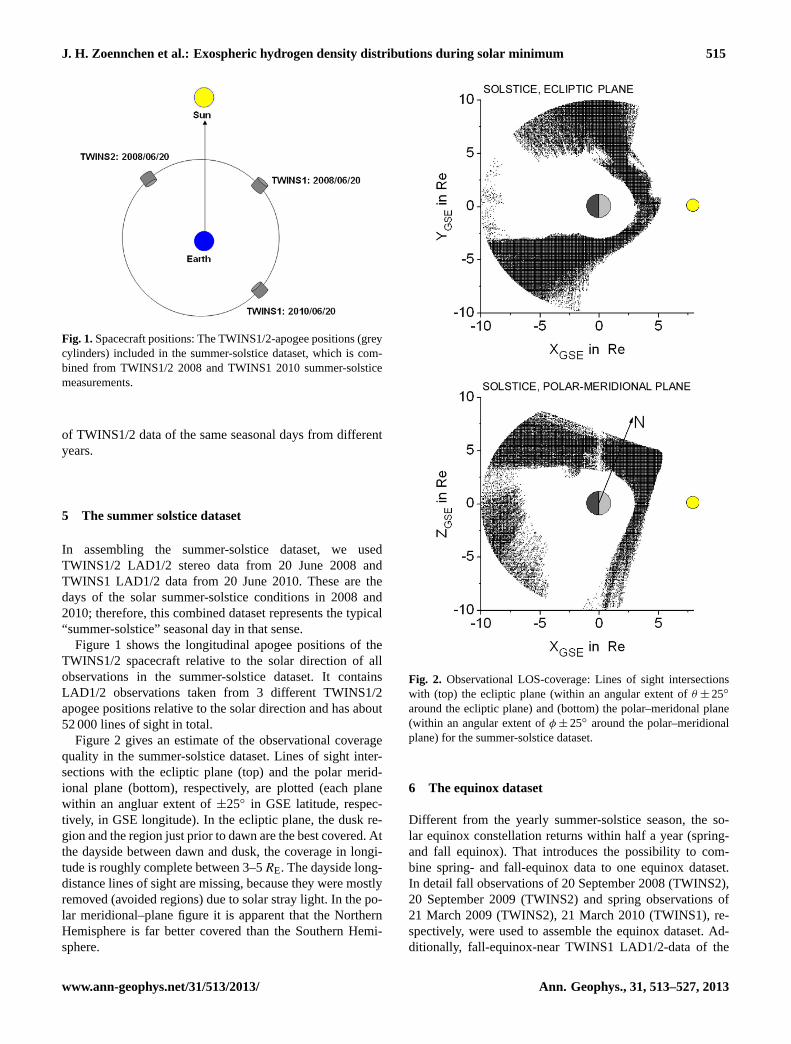
Fig. 1.Spacecraft positions: The TWINS1/2-apogee positions (greycylinders) included in the summer-solstice dataset, which is com-bined from TWINS1/2 2008 and TWINS1 2010 summer-solsticemeasurements.

of TWINS1/2 data of the same seasonal days from differentyears.

5 The summer solstice dataset

In assembling the summer-solstice dataset, we usedTWINS1/2 LAD1/2 stereo data from 20 June 2008 andTWINS1 LAD1/2 data from 20 June 2010. These are thedays of the solar summer-solstice conditions in 2008 and2010; therefore, this combined dataset represents the typical“summer-solstice” seasonal day in that sense.

Figure 1 shows the longitudinal apogee positions of theTWINS1/2 spacecraft relative to the solar direction of allobservations in the summer-solstice dataset. It containsLAD1/2 observations taken from 3 different TWINS1/2apogee positions relative to the solar direction and has about52 000 lines of sight in total.

Figure 2 gives an estimate of the observational coveragequality in the summer-solstice dataset. Lines of sight inter-sections with the ecliptic plane (top) and the polar merid-ional plane (bottom), respectively, are plotted (each planewithin an angluar extent of±25◦ in GSE latitude, respec-tively, in GSE longitude). In the ecliptic plane, the dusk re-gion and the region just prior to dawn are the best covered. Atthe dayside between dawn and dusk, the coverage in longi-tude is roughly complete between 3–5RE. The dayside long-distance lines of sight are missing, because they were mostlyremoved (avoided regions) due to solar stray light. In the po-lar meridional–plane figure it is apparent that the NorthernHemisphere is far better covered than the Southern Hemi-sphere.

Fig. 2. Observational LOS-coverage: Lines of sight intersectionswith (top) the ecliptic plane (within an angular extent ofθ ± 25◦

around the ecliptic plane) and (bottom) the polar–meridonal plane(within an angular extent ofφ ± 25◦ around the polar–meridionalplane) for the summer-solstice dataset.

6 The equinox dataset

Different from the yearly summer-solstice season, the so-lar equinox constellation returns within half a year (spring-and fall equinox). That introduces the possibility to com-bine spring- and fall-equinox data to one equinox dataset.In detail fall observations of 20 September 2008 (TWINS2),20 September 2009 (TWINS2) and spring observations of21 March 2009 (TWINS2), 21 March 2010 (TWINS1), re-spectively, were used to assemble the equinox dataset. Ad-ditionally, fall-equinox-near TWINS1 LAD1/2-data of the

www.ann-geophys.net/31/513/2013/ Ann. Geophys., 31, 513–527, 2013


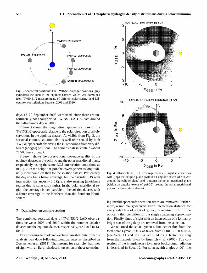
Fig. 3.Spacecraft positions: The TWINS1/2-apogee positions (greycylinders) included in the equinox dataset, which was combinedfrom TWINS1/2 measurements of different solar spring- and fall-equinox constellations between 2008 and 2010.

days 12–20 September 2008 were used, since there are un-fortunately not enough valid TWINS1 LAD1/2-data aroundthe fall-equinox day in 2008.

Figure 3 shows the longitudinal apogee positions of theTWINS1/2-spacecraft relative to the solar direction of all ob-servations in the equinox dataset. As visible from Fig. 3, theseasonal equinox situation also is well represented by bothTWINS spacecraft observing the H-geocorona from very dif-ferent (apogee) positions. The equinox dataset contains about71 500 lines of sight.

Figure 4 shows the observational coverage quality of theequinox dataset in the ecliptic and the polar meridional plane,respectively, using the same LOS-intersection conditions asin Fig. 2. In the ecliptic region the coverage here is longitudi-nally more complete than for the solstice dataset. Particularlythe dayside has a better coverage, but the dayside LOS withintersection distances> 5.5RE are also missing (avoidanceregion due to solar stray light). In the polar meridional re-gion the coverage is comparable to the solstice dataset witha better coverage in the Northern than the Southern Hemi-sphere.

7 Data selection and processing

The combined seasonal days of TWINS1/2 LAD observa-tions between 2008 and 2010 within the summer solsticedataset and the equinox dataset, respectively, are listed in Ta-ble 1.

The procedure to mark and exclude “invalid” data from theanalysis was done following identical rules as described inZoennchen et al. (2011). That means, for example, that linesof sight with an Earth-shadow intersection or those taken dur-

Fig. 4. Observational LOS-coverage: Lines of sight intersectionswith (top) the ecliptic plane (within an angular extent ofθ ± 25◦

around the ecliptic plane) and (bottom) the polar–meridonal plane(within an angular extent ofφ ± 25◦ around the polar–meridionalplane) for the equinox dataset.

ing invalid spacecraft operation times are removed. Further-more, a minimal geocentric Earth intersection distance forevery valid line of sight of≥ 3RE is required to fulfill theoptically thin condition for the single scattering approxima-tion. Finally, lines of sight with an intersection of a Lyman-α

bright star of the galaxy are removed from the selection.We obtained the solar Lyman-α line-center flux from the

total solar Lyman-α flux as taken from SORCE SOLSTICE(see Sect. 11 and Fig. 6), adjusted by a factor resultingfrom the formula given by Emerich et al. (2005). The cor-rection of the interplanetary Lyman-α background radiationis described in Sect. 12. For solar zenith angles> 90◦, the



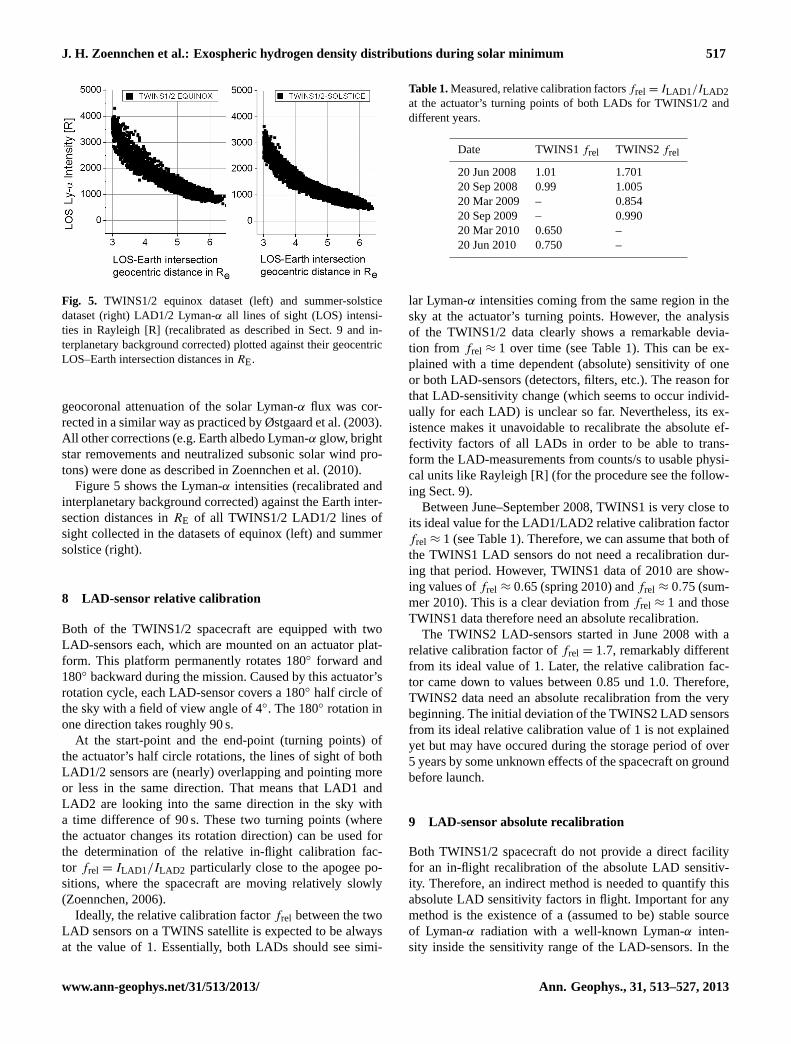
Fig. 5. TWINS1/2 equinox dataset (left) and summer-solsticedataset (right) LAD1/2 Lyman-α all lines of sight (LOS) intensi-ties in Rayleigh [R] (recalibrated as described in Sect. 9 and in-terplanetary background corrected) plotted against their geocentricLOS–Earth intersection distances inRE.

geocoronal attenuation of the solar Lyman-α flux was cor-rected in a similar way as practiced by Østgaard et al. (2003).All other corrections (e.g. Earth albedo Lyman-α glow, brightstar removements and neutralized subsonic solar wind pro-tons) were done as described in Zoennchen et al. (2010).

Figure 5 shows the Lyman-α intensities (recalibrated andinterplanetary background corrected) against the Earth inter-section distances inRE of all TWINS1/2 LAD1/2 lines ofsight collected in the datasets of equinox (left) and summersolstice (right).

8 LAD-sensor relative calibration

Both of the TWINS1/2 spacecraft are equipped with twoLAD-sensors each, which are mounted on an actuator plat-form. This platform permanently rotates 180◦ forward and180◦ backward during the mission. Caused by this actuator’srotation cycle, each LAD-sensor covers a 180◦ half circle ofthe sky with a field of view angle of 4◦. The 180◦ rotation inone direction takes roughly 90 s.

At the start-point and the end-point (turning points) ofthe actuator’s half circle rotations, the lines of sight of bothLAD1/2 sensors are (nearly) overlapping and pointing moreor less in the same direction. That means that LAD1 andLAD2 are looking into the same direction in the sky witha time difference of 90 s. These two turning points (wherethe actuator changes its rotation direction) can be used forthe determination of the relative in-flight calibration fac-tor frel = ILAD1/ILAD2 particularly close to the apogee po-sitions, where the spacecraft are moving relatively slowly(Zoennchen, 2006).

Ideally, the relative calibration factorfrel between the twoLAD sensors on a TWINS satellite is expected to be alwaysat the value of 1. Essentially, both LADs should see simi-

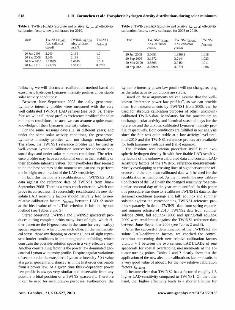
Table 1.Measured, relative calibration factorsfrel = ILAD1/ILAD2at the actuator’s turning points of both LADs for TWINS1/2 anddifferent years.

Date TWINS1frel TWINS2frel

20 Jun 2008 1.01 1.70120 Sep 2008 0.99 1.00520 Mar 2009 – 0.85420 Sep 2009 – 0.99020 Mar 2010 0.650 –20 Jun 2010 0.750 –

lar Lyman-α intensities coming from the same region in thesky at the actuator’s turning points. However, the analysisof the TWINS1/2 data clearly shows a remarkable devia-tion from frel ≈ 1 over time (see Table 1). This can be ex-plained with a time dependent (absolute) sensitivity of oneor both LAD-sensors (detectors, filters, etc.). The reason forthat LAD-sensitivity change (which seems to occur individ-ually for each LAD) is unclear so far. Nevertheless, its ex-istence makes it unavoidable to recalibrate the absolute ef-fectivity factors of all LADs in order to be able to trans-form the LAD-measurements from counts/s to usable physi-cal units like Rayleigh [R] (for the procedure see the follow-ing Sect. 9).

Between June–September 2008, TWINS1 is very close toits ideal value for the LAD1/LAD2 relative calibration factorfrel ≈ 1 (see Table 1). Therefore, we can assume that both ofthe TWINS1 LAD sensors do not need a recalibration dur-ing that period. However, TWINS1 data of 2010 are show-ing values offrel ≈ 0.65 (spring 2010) andfrel ≈ 0.75 (sum-mer 2010). This is a clear deviation fromfrel ≈ 1 and thoseTWINS1 data therefore need an absolute recalibration.

The TWINS2 LAD-sensors started in June 2008 with arelative calibration factor offrel = 1.7, remarkably differentfrom its ideal value of 1. Later, the relative calibration fac-tor came down to values between 0.85 und 1.0. Therefore,TWINS2 data need an absolute recalibration from the verybeginning. The initial deviation of the TWINS2 LAD sensorsfrom its ideal relative calibration value of 1 is not explainedyet but may have occured during the storage period of over5 years by some unknown effects of the spacecraft on groundbefore launch.

9 LAD-sensor absolute recalibration

Both TWINS1/2 spacecraft do not provide a direct facilityfor an in-flight recalibration of the absolute LAD sensitiv-ity. Therefore, an indirect method is needed to quantify thisabsolute LAD sensitivity factors in flight. Important for anymethod is the existence of a (assumed to be) stable sourceof Lyman-α radiation with a well-known Lyman-α inten-sity inside the sensitivity range of the LAD-sensors. In the



Table 2.TWINS1-LAD (absolute and relativefrel,recal) effectivitycalibration factors, newly calibrated for 2010.

Date TWINS1ηLAD1 TWINS1ηLAD2 TWINS1Abs. calfactor Abs. calfactor frel,recalcts/s/R cts/s/R

20 Jun 2008 2.205 2.166 1.020 Sep 2008 2.205 2.166 1.020 Mar 2010 1.03635 1.6245 1.01820 Jun 2010 1.21275 1.58118 0.9778

following we will discuss a recalibration method based onexospheric hydrogen Lyman-α intensity profiles under stablesolar activity conditions:

Between June–September 2008 the daily geocoronalLyman-α intensity profiles were measured with the verywell calibrated TWINS1 LAD sensors (see Sect. 8). There-fore we will call those profiles “reference profiles” for solarminimum conditions, because we can assume a quite exactknowledge of their Lyman-α intensity values.

For the same seasonal days (i.e. in different years) andunder the same solar activity conditions, the geocoronalLyman-α intensity profiles will not change remarkably.Therefore, the TWINS1 reference profiles can be used aswell-known Lyman-α calibration sources for adequate sea-sonal days and under solar minimum conditions. The refer-ence profiles may have an additional error in their stability ortheir absolute intensity values, but nevertheless they seemedto be the best sources at the moment we can use to performthe in-flight recalibration of the LAD sensitivity.

In fact, this method is a recalibration of TWINS1/2 LADdata against the reference data of TWINS1 from June–September 2008. There is a cross check criterion, which canprove its correctness: If successfully recalibrated the new ab-solute LAD sensitivity factors should naturally lead to newrelative calibration factorsfrel,recal between LAD1/2 stableat the ideal value of≈ 1. This criterion is fulfilled by ourmethod (see Tables 2 and 3).

Stereo observing TWINS1 and TWINS2 spacecraft pro-duces during complete orbits many lines of sight, which ei-ther penetrate the H-geocorona in the same (or very nearby)spatial regions or which cross each other. In the mathemati-cal sense, those overlapping or crossing lines of sight repre-sent border conditions in the tomographic enfolding, whichconstrain the possible solution space in a very effective way.Another constraining factor is the power law dominated geo-coronal Lyman-α intensity profile. Despite angular variationsof second order the exospheric Lyman-α intensityI (r) valueat a given geocentric distancer is in the first order deriveablefrom a power law. At a given time thisr-dependent powerlaw profile is always very similar and observable from anypossible orbital position of a TWINS spacecraft. Thereforeit can be used for recalibration purposes. Furthermore, the

Table 3.TWINS2-LAD (absolute and relativefrel,recal) effectivitycalibration factors, newly calibrated for 2008 to 2010.

Date TWINS2ηLAD1 TWINS2ηLAD2 TWINS2Abs. calfactor Abs. calfactor frel,recalcts/s/R cts/s/R

20 Jun 2008 3.0651 1.83633 1.01820 Sep 2008 3.1372 3.2144 1.02320 Mar 2009 2.5603 3.0454 1.01120 Sep 2009 3.02904 3.0771 1.006

Lyman-α intensity power law profile will not change as longas the solar activity conditions are stable.

Based on these arguments we can assume that the well-known “reference power law profiles”, as we can providethem from measurements by TWINS1 from 2008, can beused for absolute calibration purposes of other (unknown)calibrated TWINS-data. Mandatory for this practice are anunchanged solar activity and identical seasonal days for thereference and the unkown calibrated Lyman-α intensity pro-file, respectively. Both conditions are fulfilled in our analysissince the Sun was quite stable at a low activity level untilmid-2010 and the TWINS1 reference profiles are availablefor both (summer-) solstice and (fall-) equinox.

The absolute recalibration procedure itself is an exo-spheric hydrogen density fit with free fitable LAD sensitiv-ity factors of the unknown calibrated data and constant LADsensitivity factors of the TWINS1 reference measurements.Mostly overlapping or crossing lines of sight between the ref-erence and the unknown calibrated data will be used for therecalibration as mentioned. As the fit result, the new calibra-tion factors of the LAD with the changed sensitivity for a par-ticular seasonal day of the year are quantified. In this paperthis procedure was done to recalibrate TWINS1/2 data for theseasonal conditions (spring- and fall) equinox and summersolstice against the corresponding TWINS1-reference pro-files separately. In detail, TWINS1 data from spring equinoxand summer solstice of 2010, TWINS2 data from summersolstice 2008, fall equinox 2008 and spring-/fall equinox2009 were recalibrated against the TWINS1 reference databetween June–September 2008 (see Tables 2 und 3).

After the successful determination of the TWINS1/2 ab-solute LAD-calibration factors, we checked the controlcriterion concerning their new relative calibration factorsfrel,recal≈ 1 between the two sensors LAD1/LAD2 of onespacecraft for spatial overlapping measurements at the ac-tuator turning points. Tables 2 and 3 clearly show that theapplication of the new absolute calibrations factors results ina very good value of about 1 for the new relative calibrationfactorsfrel,recal.

It became clear that TWINS2 has a factor of roughly 1.5higher LAD-sensitivity compared to TWINS1. On the otherhand, that higher effectivity leads to a shorter lifetime for



the TWINS2 LAD because of the higher detector exhaustingrate.

As a methodical test, the absolute calibration procedurewas performed with the known exospheric hydrogen dis-tribution from Hodges (1994) and testwise shifted (decal-ibrated) LAD-sensitivity factors of one satellite. The sen-sitivity factors of the other satellite were treated as con-stant. In every test case the method resulted with the correct(unshifted) sensitivity factors of the before testwise-shiftedLAD.

10 Scattering phase function correction

Brandt and Chamberlain (1959) described an angular inten-sity dependenceI (α) of the scattered Lyman-α photons withrespect to the direction of the incoming (solar) Lyman-α pho-tons as follows:

I (α) = 1+1

4

(2

3− sin2(α)

). (1)

The maximal (percentage) variation of this angular depen-dence compared to the isotropic case is+16.7 % for α =

0◦, 180◦ and −8.3 % for α = 90◦, 270◦. That means, inother words, there is a relatively small preference for for-ward/backward scattering in the Lyman-α resonant scatteringprocess. We correct our model scattering calculations by theinclusion of the phase function from Eq. (1). Since the nu-merical corrections due to this phase function are relativelysmall, our test fits of the neutral exospheric H-density distri-bution with and without consideration of the phase functionshow very small quantitative differences.

11 Solar conditions

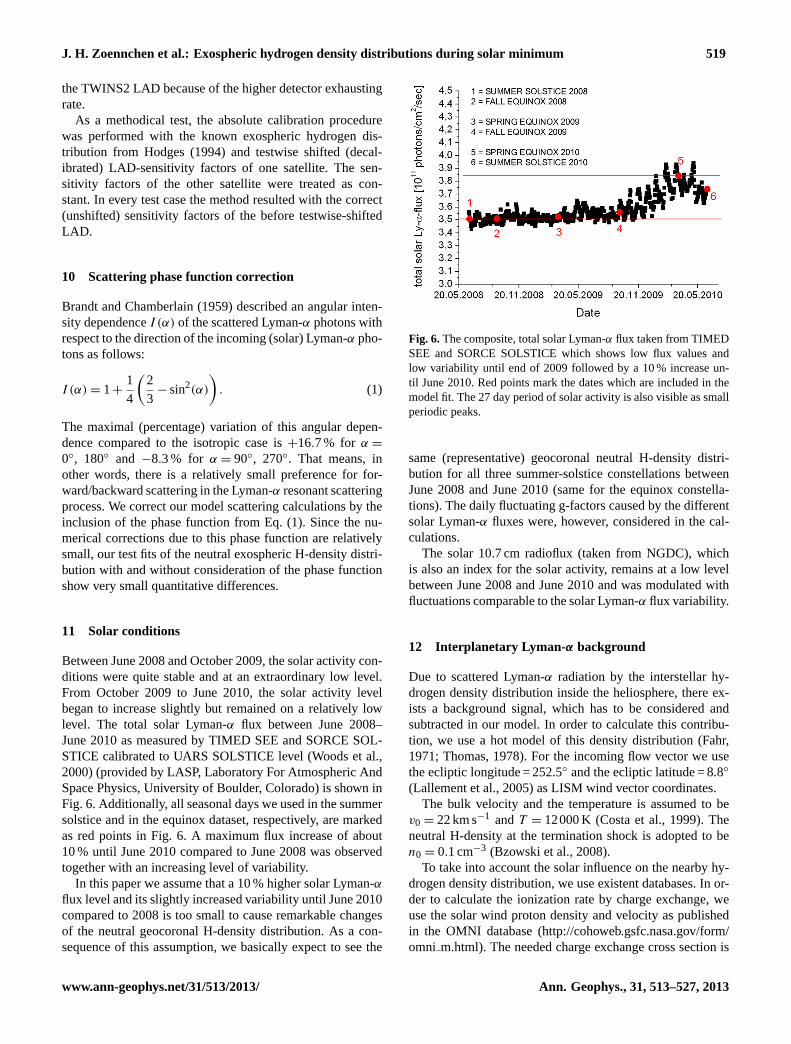
Between June 2008 and October 2009, the solar activity con-ditions were quite stable and at an extraordinary low level.From October 2009 to June 2010, the solar activity levelbegan to increase slightly but remained on a relatively lowlevel. The total solar Lyman-α flux between June 2008–June 2010 as measured by TIMED SEE and SORCE SOL-STICE calibrated to UARS SOLSTICE level (Woods et al.,2000) (provided by LASP, Laboratory For Atmospheric AndSpace Physics, University of Boulder, Colorado) is shown inFig. 6. Additionally, all seasonal days we used in the summersolstice and in the equinox dataset, respectively, are markedas red points in Fig. 6. A maximum flux increase of about10 % until June 2010 compared to June 2008 was observedtogether with an increasing level of variability.

In this paper we assume that a 10 % higher solar Lyman-α

flux level and its slightly increased variability until June 2010compared to 2008 is too small to cause remarkable changesof the neutral geocoronal H-density distribution. As a con-sequence of this assumption, we basically expect to see the

Fig. 6.The composite, total solar Lyman-α flux taken from TIMEDSEE and SORCE SOLSTICE which shows low flux values andlow variability until end of 2009 followed by a 10 % increase un-til June 2010. Red points mark the dates which are included in themodel fit. The 27 day period of solar activity is also visible as smallperiodic peaks.

same (representative) geocoronal neutral H-density distri-bution for all three summer-solstice constellations betweenJune 2008 and June 2010 (same for the equinox constella-tions). The daily fluctuating g-factors caused by the differentsolar Lyman-α fluxes were, however, considered in the cal-culations.

The solar 10.7 cm radioflux (taken from NGDC), whichis also an index for the solar activity, remains at a low levelbetween June 2008 and June 2010 and was modulated withfluctuations comparable to the solar Lyman-α flux variability.

12 Interplanetary Lyman-α background

Due to scattered Lyman-α radiation by the interstellar hy-drogen density distribution inside the heliosphere, there ex-ists a background signal, which has to be considered andsubtracted in our model. In order to calculate this contribu-tion, we use a hot model of this density distribution (Fahr,1971; Thomas, 1978). For the incoming flow vector we usethe ecliptic longitude = 252.5◦ and the ecliptic latitude = 8.8◦

(Lallement et al., 2005) as LISM wind vector coordinates.The bulk velocity and the temperature is assumed to be

v0 = 22 km s−1 andT = 12000 K (Costa et al., 1999). Theneutral H-density at the termination shock is adopted to ben0 = 0.1 cm−3 (Bzowski et al., 2008).

To take into account the solar influence on the nearby hy-drogen density distribution, we use existent databases. In or-der to calculate the ionization rate by charge exchange, weuse the solar wind proton density and velocity as publishedin the OMNI database (http://cohoweb.gsfc.nasa.gov/form/omni m.html). The needed charge exchange cross section is


http://cohoweb.gsfc.nasa.gov/form/omni_m.html

http://cohoweb.gsfc.nasa.gov/form/omni_m.html


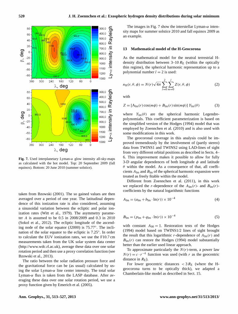
Fig. 7. Used interplanetary Lyman-α glow intensity all-sky-mapsas calculated with the hot model. Top: 20 September 2009 (fallequinox). Bottom: 20 June 2010 (summer solstice).

taken from Bzowski (2001). The so gained values are thenaveraged over a period of one year. The latitudinal depen-dence of this ionization rate is also considered, assuminga sinusoidal variation between the ecliptic and polar ion-ization rates (Witt et al., 1979). The asymmetry parame-ter A is assumed to be 0.5 in 2008/2009 and 0.3 in 2010(Sokol et al., 2012). The ecliptic longitude of the ascend-ing node of the solar equator (J2000) is 75.77◦. The incli-nation of the solar equator to the ecliptic is 7.25◦. In orderto calculate the EUV ionization rates, we use the F10.7 cmmeasurements taken from the UK solar system data center(http://www.wdc.rl.ac.uk), average these data over one solarrotation period and then use a proxy correlation function (seeBzowski et al., 2013).

The ratio between the solar radiation pressure force andthe gravitational force can be (as usual) calculated by us-ing the solar Lyman-α line center intensity. The total solarLyman-α flux is taken from the LASP database. After av-eraging these data over one solar rotation period, we use aproxy function given by Emerich et al. (2005).

The images in Fig. 7 show the interstellar Lyman-α inten-sity maps for summer solstice 2010 and fall equinox 2009 asan example.

13 Mathematical model of the H-Geocorona

As the mathematical model for the neutral terrestrial H-density distribution between 3–10RE (within the opticallythin regime), the spherical harmonic representation up to apolynomial numberl = 2 is used:

nH(r,θ,φ) = N(r)√

4π

2∑l=0

l∑m=0

Z(r,θ,φ) (2)

with

Z = [A lm(r)cos(mφ)+ Blm(r)sin(mφ)] Ylm(θ) (3)

where Ylm(θ) are the spherical harmonic Legendre-polynomials. This coefficient parameterization is based onthe simplified version of the Hodges (1994) model that wasemployed by Zoennchen et al. (2010) and is also used withsome modifications in this work.

The geocoronal coverage in this analysis could be im-proved tremendously by the involvement of (partly stereo)data from TWINS1 and TWINS2 using LAD-lines of sightfrom very different orbital positions as described in Sects. 4–6. This improvement makes it possible to allow for fully3-D angular dependences of both longitudeφ and latitudeθ within the model. As a consequence of that, all coeffi-cientsAlm andBlm of the spherical harmonic expansion weretreated as freely fitable within the model.

Different from Zoennchen et al. (2011), in this workwe replaced ther-dependence of theAlm(r)- and Blm(r)-coefficients by the natural logarithmic functions

Alm = (alm + blm · ln(r)) × 10−4 (4)

Blm = (plm + qlm · ln(r)) × 10−4 (5)

with constantA00 = 1. Restoration tests of the Hodges(1994) model based on TWINS1/2 lines of sight broughtthe result that this logarithmicr-dependence ofAlm(r) andBlm(r) can restore the Hodges (1994) model substantiallybetter than the earlier used linear approach.

To approximate particularly theN(r)-term, a power lawN(r) = c · r−k function was used (withr as the geocentricdistance inRE).

For lower geocentric distances< 3RE (where the H-geocorona turns to be optically thick), we adapted aChamberlain-like model as described in Sect. 15.


http://www.wdc.rl.ac.uk


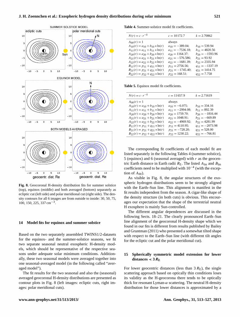
Fig. 8. Geocoronal H-density distribution fits for summer solstice(top), equinox (middle) and both averaged (bottom) separately asecliptic cut (left side) and polar meridional cut (right side). The den-sity contours for all 6 images are from outside to inside: 30, 50, 75,100, 150, 225, 337 cm−3.

14 Model fits for equinox and summer solstice

Based on the two separately assembled TWINS1/2-datasetsfor the equinox- and the summer-solstice seasons, we fittwo separate seasonal neutral exospheric H-density mod-els, which should be representative of the respective sea-sons under adequate solar minimum conditions. Addition-ally, these two seasonal models were averaged together intoone seasonal-averaged model (in the following called “aver-aged model”).

The fit results for the two seasonal and also the (seasonal)averaged geocoronal H-density distributions are presented ascontour plots in Fig. 8 (left images: ecliptic cuts, right im-ages: polar meridional cuts).

Table 4.Summer-solstice model fit coefficients.

N(r) = c · r−k c = 10172.7 k = 2.70862

A00(r) = 1 alwaysA10(r) = a10+ b10∗ ln(r) a10 = −389.04; b10 = 539.94A11(r) = a11+ b11∗ ln(r) a11 = −7536.18; b11 = 4820.56A20(r) = a20+ b20∗ ln(r) a20 = 1164.37; b20 = −1593.96A21(r) = a21+ b21∗ ln(r) a21 = −576.586; b21 = 93.92A22(r) = a22+ b22∗ ln(r) a22 = −1681.39; b22 = 2335.94B11(r) = p11+ q11∗ ln(r) p11 = 2756.56; q11 = −1337.19B21(r) = p21+ q21∗ ln(r) p21 = −1745.40; q21 = 1414.75B22(r) = p22+ q22∗ ln(r) p22 = 168.51; q22 = 7.758

Table 5.Equinox model fit coefficients.

N(r) = c · r−k c = 11657.9 k = 2.71619

A00(r) = 1 alwaysA10(r) = a10+ b10∗ ln(r) a10 = −6.075; b10 = 334.16A11(r) = a11+ b11∗ ln(r) a11 = −2994.08; b11 = 892.39A20(r) = a20+ b20∗ ln(r) a20 = 1759.70; b20 = −1816.44A21(r) = a21+ b21∗ ln(r) a21 = 1048.91; b21 = −669.89A22(r) = a22+ b22∗ ln(r) a22 = −4969.92; b22 = 4281.99B11(r) = p11+ q11∗ ln(r) p11 = 4110.95; q11 = −2073.98B21(r) = p21+ q21∗ ln(r) p21 = −728.20; q21 = 528.00B22(r) = p22+ q22∗ ln(r) p22 = 1230.22; q22 = −766.81

The corresponding fit coefficients of each model fit arelisted separately in the following Tables 4 (summer solstice),5 (equinox) and 6 (seasonal averaged) withr as the geocen-tric Earth distance in Earth radiiRE. The listedAlm andBlmcoefficients need to be multiplied with 10−4 (with the excep-tion of A00).

As visible in Fig. 8, the angular structures of the exo-spheric hydrogen distributions seem to be strongly alignedwith the Earth–Sun line. This alignment is manifest in thefit results independent from the season. A cigar-like shape ofthe density structure (in both cuts) is obvious. This encour-ages our expectation that the shape of the terrestrial neutralH exosphere is mainly Sun-controlled.

The different angular dependences are discussed in thefollowing Sects. 18–21. The clearly pronounced Earth–Sunline alignment of the geocoronal H-density shape which wefound in our fits is different from results published by Baileyand Gruntman (2011) who presented a somewhat tilted shapewith respect to the Earth–Sun line (with different tilt anglesfor the ecliptic cut and the polar meridional cut).

15 Spherically symmetric model extension for lowerdistances< 3RE

For lower geocentric distances (less than 3RE), the singlescattering approach based on optically thin conditions losesits validity as the H-geocorona there tends to be opticallythick for resonant Lyman-α scattering. The neutral H-densitydistribution for those lower distances is approximated by a



Table 6.Seasonal averaged model fit coefficients.

N(r) = c · r−k c = 10915.119 k = 2.7126401

A00(r) = 1 alwaysA10(r) = a10+ b10∗ ln(r) a10 = −185.29; b10 = 430.44A11(r) = a11+ b11∗ ln(r) a11 = −5125.25; b11 = 2735.51A20(r) = a20+ b20∗ ln(r) a20 = 1481.46; b20 = −1712.69A21(r) = a21+ b21∗ ln(r) a21 = 288.61; b21 = −312.91A22(r) = a22+ b22∗ ln(r) a22 = −3430.27; b22 = 3370.85B11(r) = p11+ q11∗ ln(r) p11 = 3477.09; q11 = −1729.22B21(r) = p21+ q21∗ ln(r) p21 = −1205.50; q21 = 944.08B22(r) = p22+ q22∗ ln(r) p22 = 732.60; q22 = −403.69

spherically symmetric (Chamberlain, 1963)-like model:

nH(r) = a · exp(b/r). (6)

We use this Chamberlain-like model as an extension forr < 3RE of our spherically harmonic model (Eq. 2). Thatcombined (extended) model provides H-density values from≈ 1000 km altitude up to 10RE geocentric distance. In orderto get a (nearly) continuous H-density interface between thetwo models atr = 3RE, we fit the Chamberlain-like modelcoefficientsa andb to

a = 32.745 ; b = 8.3845. (7)

The used two fit constraints are an H-density value at 1RE,as published by (Carruthers et al., 1976), and the sphericallysymmetric averaged H-density value from our seasonally av-eraged model at the interface geocentric distance of 3RE.

The H-density profile fit of the Chamberlain-like modeland its adaption to our averaged spherical harmonic exten-sion model profile at 3RE is shown in Fig. 14 in segment (A).

16 Interpolation of a daily H-density distribution forquiet solar minimum conditions

Since the geocoronal H-density distribution is changing peri-odically between the seasonal equinox and solstice, it seemsto be reliable to calculate the H-density distribution for a par-ticular day of the year by an (linear and time weighted) in-terpolation of the two seasonal H-density distributions wherethis day is situated in between.

In Sect. 14 we present neutral geocoronal H-density fitsfor equinox and summer solstice separately. Since we donot have reliable winter-solstice data from TWINS betweenJune 2008 and June 2010, we assume, instead, that thewinter-solstice model is a z-axis inverted summer-solstice H-density model, which was also practiced by Hodges (1994).Using this assumption a winter-solstice model for solar quietconditions can be easily calculated from our summer-solsticemodel doing a z-axis inversion.

From that point all the neccessary seasonal equinox,summer- and winter solstices are known and a geocoronal

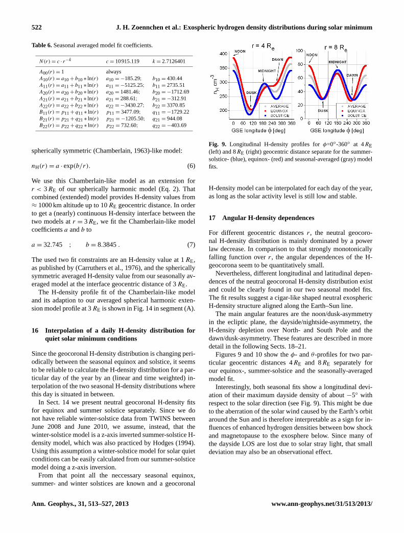
Fig. 9. Longitudinal H-density profiles forφ=0◦-360◦ at 4RE(left) and 8RE (right) geocentric distance separate for the summer-solstice- (blue), equinox- (red) and seasonal-averaged (gray) modelfits.

H-density model can be interpolated for each day of the year,as long as the solar activity level is still low and stable.

17 Angular H-density dependences

For different geocentric distancesr, the neutral geocoro-nal H-density distribution is mainly dominated by a powerlaw decrease. In comparison to that strongly monotonicallyfalling function overr, the angular dependences of the H-geocorona seem to be quantitatively small.

Nevertheless, different longitudinal and latitudinal depen-dences of the neutral geocoronal H-density distribution existand could be clearly found in our two seasonal model fits.The fit results suggest a cigar-like shaped neutral exosphericH-density structure aligned along the Earth–Sun line.

The main angular features are the noon/dusk-asymmetryin the ecliptic plane, the dayside/nightside-asymmetry, theH-density depletion over North- and South Pole and thedawn/dusk-asymmetry. These features are described in moredetail in the following Sects. 18–21.

Figures 9 and 10 show theφ- andθ -profiles for two par-ticular geocentric distances 4RE and 8RE separately forour equinox-, summer-solstice and the seasonally-averagedmodel fit.

Interestingly, both seasonal fits show a longitudinal devi-ation of their maximum dayside density of about−5◦ withrespect to the solar direction (see Fig. 9). This might be dueto the aberration of the solar wind caused by the Earth’s orbitaround the Sun and is therefore interpretable as a sign for in-fluences of enhanced hydrogen densities between bow shockand magnetopause to the exosphere below. Since many ofthe dayside LOS are lost due to solar stray light, that smalldeviation may also be an observational effect.



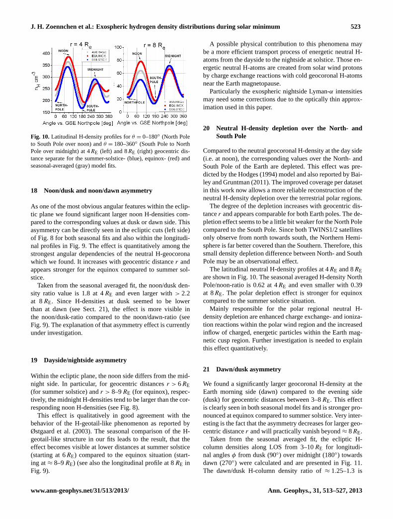
Fig. 10.Latitudinal H-density profiles forθ = 0–180◦ (North Poleto South Pole over noon) andθ = 180–360◦ (South Pole to NorthPole over midnight) at 4RE (left) and 8RE (right) geocentric dis-tance separate for the summer-solstice- (blue), equinox- (red) andseasonal-averaged (gray) model fits.

18 Noon/dusk and noon/dawn asymmetry

As one of the most obvious angular features within the eclip-tic plane we found significant larger noon H-densities com-pared to the corresponding values at dusk or dawn side. Thisasymmetry can be directly seen in the ecliptic cuts (left side)of Fig. 8 for both seasonal fits and also within the longitudi-nal profiles in Fig. 9. The effect is quantitatively among thestrongest angular dependencies of the neutral H-geocoronawhich we found. It increases with geocentric distancer andappears stronger for the equinox compared to summer sol-stice.

Taken from the seasonal averaged fit, the noon/dusk den-sity ratio value is 1.8 at 4RE and even larger with> 2.2at 8RE. Since H-densities at dusk seemed to be lowerthan at dawn (see Sect. 21), the effect is more visible inthe noon/dusk-ratio compared to the noon/dawn-ratio (seeFig. 9). The explanation of that asymmetry effect is currentlyunder investigation.

19 Dayside/nightside asymmetry

Within the ecliptic plane, the noon side differs from the mid-night side. In particular, for geocentric distancesr > 6RE(for summer solstice) andr > 8–9RE (for equinox), respec-tively, the midnight H-densities tend to be larger than the cor-responding noon H-densities (see Fig. 8).

This effect is qualitatively in good agreement with thebehavior of the H-geotail-like phenomenon as reported byØstgaard et al. (2003). The seasonal comparison of the H-geotail-like structure in our fits leads to the result, that theeffect becomes visible at lower distances at summer solstice(starting at 6RE) compared to the equinox situation (start-ing at≈ 8–9RE) (see also the longitudinal profile at 8RE inFig. 9).

A possible physical contribution to this phenomena maybe a more efficient transport process of energetic neutral H-atoms from the dayside to the nightside at solstice. Those en-ergetic neutral H-atoms are created from solar wind protonsby charge exchange reactions with cold geocoronal H-atomsnear the Earth magnetopause.

Particularly the exospheric nightside Lyman-α intensitiesmay need some corrections due to the optically thin approx-imation used in this paper.

20 Neutral H-density depletion over the North- andSouth Pole

Compared to the neutral geocoronal H-density at the day side(i.e. at noon), the corresponding values over the North- andSouth Pole of the Earth are depleted. This effect was pre-dicted by the Hodges (1994) model and also reported by Bai-ley and Gruntman (2011). The improved coverage per datasetin this work now allows a more reliable reconstruction of theneutral H-density depletion over the terrestrial polar regions.

The degree of the depletion increases with geocentric dis-tancer and appears comparable for both Earth poles. The de-pletion effect seems to be a little bit weaker for the North Polecompared to the South Pole. Since both TWINS1/2 satellitesonly observe from north towards south, the Northern Hemi-sphere is far better covered than the Southern. Therefore, thissmall density depletion difference between North- and SouthPole may be an observational effect.

The latitudinal neutral H-density profiles at 4RE and 8REare shown in Fig. 10. The seasonal averaged H-density NorthPole/noon-ratio is 0.62 at 4RE and even smaller with 0.39at 8RE. The polar depletion effect is stronger for equinoxcompared to the summer solstice situation.

Mainly responsible for the polar regional neutral H-density depletion are enhanced charge exchange- and ioniza-tion reactions within the polar wind region and the increasedinflow of charged, energetic particles within the Earth mag-netic cusp region. Further investigation is needed to explainthis effect quantitatively.

21 Dawn/dusk asymmetry

We found a significantly larger geocoronal H-density at theEarth morning side (dawn) compared to the evening side(dusk) for geocentric distances between 3–8RE. This effectis clearly seen in both seasonal model fits and is stronger pro-nounced at equinox compared to summer solstice. Very inter-esting is the fact that the asymmetry decreases for larger geo-centric distancer and will practically vanish beyond≈ 8RE.

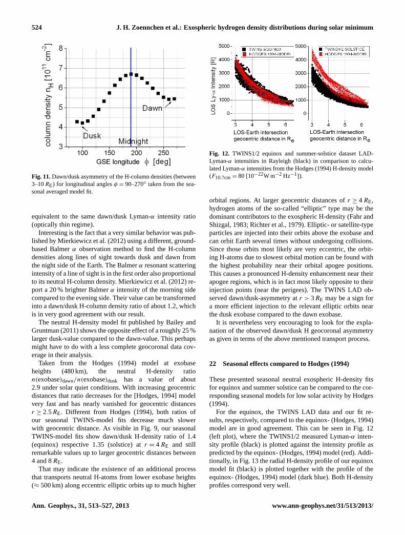
Taken from the seasonal averaged fit, the ecliptic H-column densities along LOS from 3–10RE for longitudi-nal anglesφ from dusk (90◦) over midnight (180◦) towardsdawn (270◦) were calculated and are presented in Fig. 11.The dawn/dusk H-column density ratio of≈ 1.25–1.3 is



Fig. 11.Dawn/dusk asymmetry of the H-column densities (between3–10RE) for longitudinal anglesφ = 90–270◦ taken from the sea-sonal averaged model fit.

equivalent to the same dawn/dusk Lyman-α intensity ratio(optically thin regime).

Interesting is the fact that a very similar behavior was pub-lished by Mierkiewicz et al. (2012) using a different, ground-based Balmerα observation method to find the H-columndensities along lines of sight towards dusk and dawn fromthe night side of the Earth. The Balmerα resonant scatteringintensity of a line of sight is in the first order also proportionalto its neutral H-column density. Mierkiewicz et al. (2012) re-port a 20 % brighter Balmerα intensity of the morning sidecompared to the evening side. Their value can be transformedinto a dawn/dusk H-column density ratio of about 1.2, whichis in very good agreement with our result.

The neutral H-density model fit published by Bailey andGruntman (2011) shows the opposite effect of a roughly 25 %larger dusk-value compared to the dawn-value. This perhapsmight have to do with a less complete geocoronal data cov-erage in their analysis.

Taken from the Hodges (1994) model at exobaseheights (480 km), the neutral H-density ration(exobase)dawn/n(exobase)dusk has a value of about2.9 under solar quiet conditions. With increasing geocentricdistances that ratio decreases for the [Hodges, 1994] modelvery fast and has nearly vanished for geocentric distancesr ≥ 2.5RE. Different from Hodges (1994), both ratios ofour seasonal TWINS-model fits decrease much slowerwith geocentric distance. As visible in Fig. 9, our seasonalTWINS-model fits show dawn/dusk H-density ratio of 1.4(equinox) respective 1.35 (solstice) atr = 4RE and stillremarkable values up to larger geocentric distances between4 and 8RE.

That may indicate the existence of an additional processthat transports neutral H-atoms from lower exobase heights(≈ 500 km) along eccentric elliptic orbits up to much higher

Fig. 12. TWINS1/2 equinox and summer-solstice dataset LAD-Lyman-α intensities in Rayleigh (black) in comparison to calcu-lated Lyman-α intensities from the Hodges (1994) H-density model(F10.7cm= 80 [10−22W m−2 Hz−1

]).

orbital regions. At larger geocentric distances ofr ≥ 4RE,hydrogen atoms of the so-called “elliptic” type may be thedominant contributors to the exospheric H-density (Fahr andShizgal, 1983; Richter et al., 1979). Elliptic- or satellite-typeparticles are injected into their orbits above the exobase andcan orbit Earth several times without undergoing collisions.Since those orbits most likely are very eccentric, the orbit-ing H-atoms due to slowest orbital motion can be found withthe highest probability near their orbital apogee positions.This causes a pronounced H-density enhancement near theirapogee regions, which is in fact most likely opposite to theirinjection points (near the perigees). The TWINS LAD ob-served dawn/dusk-asymmetry atr > 3RE may be a sign fora more efficient injection to the relevant elliptic orbits nearthe dusk exobase compared to the dawn exobase.

It is nevertheless very encouraging to look for the expla-nation of the observed dawn/dusk H geocoronal asymmetryas given in terms of the above mentioned transport process.

22 Seasonal effects compared to Hodges (1994)

These presented seasonal neutral exospheric H-density fitsfor equinox and summer solstice can be compared to the cor-responding seasonal models for low solar activity by Hodges(1994).

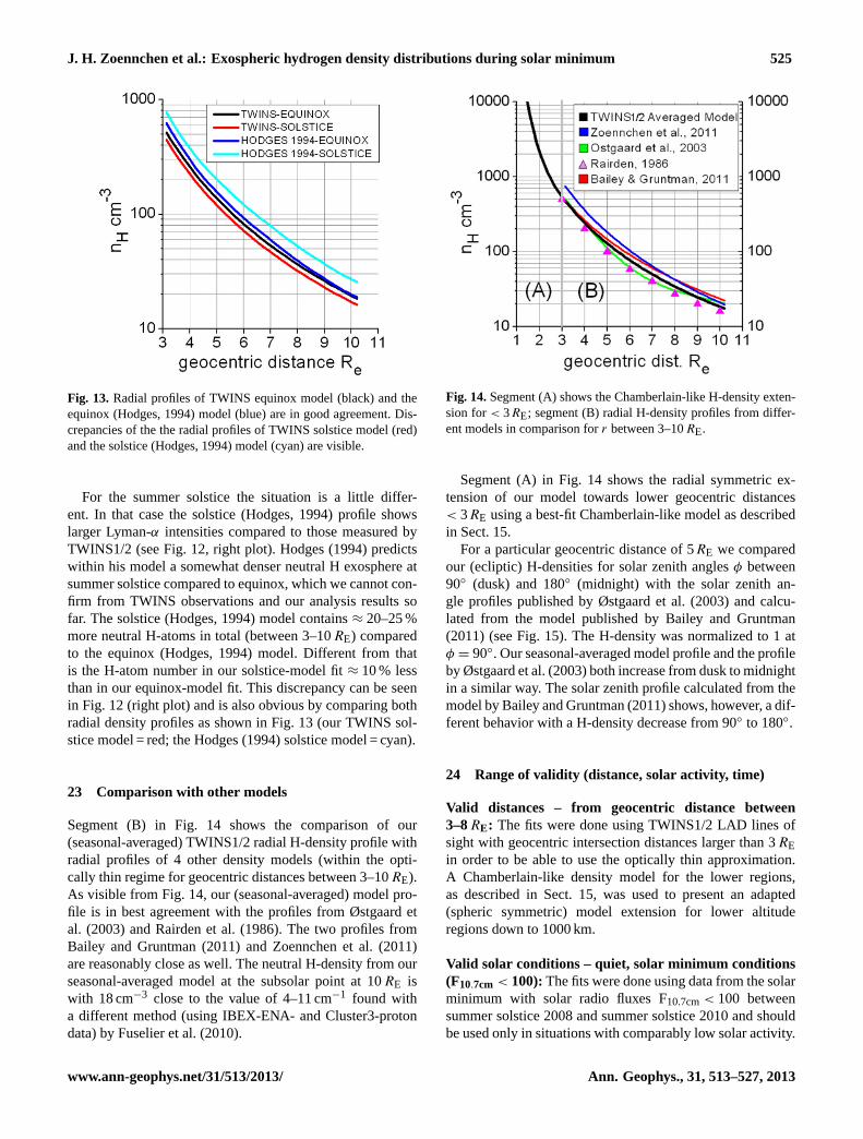
For the equinox, the TWINS LAD data and our fit re-sults, respectively, compared to the equinox- (Hodges, 1994)model are in good agreement. This can be seen in Fig. 12(left plot), where the TWINS1/2 measured Lyman-α inten-sity profile (black) is plotted against the intensity profile aspredicted by the equinox- (Hodges, 1994) model (red). Addi-tionally, in Fig. 13 the radial H-density profile of our equinoxmodel fit (black) is plotted together with the profile of theequinox- (Hodges, 1994) model (dark blue). Both H-densityprofiles correspond very well.



Fig. 13. Radial profiles of TWINS equinox model (black) and theequinox (Hodges, 1994) model (blue) are in good agreement. Dis-crepancies of the the radial profiles of TWINS solstice model (red)and the solstice (Hodges, 1994) model (cyan) are visible.

For the summer solstice the situation is a little differ-ent. In that case the solstice (Hodges, 1994) profile showslarger Lyman-α intensities compared to those measured byTWINS1/2 (see Fig. 12, right plot). Hodges (1994) predictswithin his model a somewhat denser neutral H exosphere atsummer solstice compared to equinox, which we cannot con-firm from TWINS observations and our analysis results sofar. The solstice (Hodges, 1994) model contains≈ 20–25 %more neutral H-atoms in total (between 3–10RE) comparedto the equinox (Hodges, 1994) model. Different from thatis the H-atom number in our solstice-model fit≈ 10 % lessthan in our equinox-model fit. This discrepancy can be seenin Fig. 12 (right plot) and is also obvious by comparing bothradial density profiles as shown in Fig. 13 (our TWINS sol-stice model = red; the Hodges (1994) solstice model = cyan).

23 Comparison with other models

Segment (B) in Fig. 14 shows the comparison of our(seasonal-averaged) TWINS1/2 radial H-density profile withradial profiles of 4 other density models (within the opti-cally thin regime for geocentric distances between 3–10RE).As visible from Fig. 14, our (seasonal-averaged) model pro-file is in best agreement with the profiles from Østgaard etal. (2003) and Rairden et al. (1986). The two profiles fromBailey and Gruntman (2011) and Zoennchen et al. (2011)are reasonably close as well. The neutral H-density from ourseasonal-averaged model at the subsolar point at 10RE iswith 18 cm−3 close to the value of 4–11 cm−1 found witha different method (using IBEX-ENA- and Cluster3-protondata) by Fuselier et al. (2010).

Fig. 14.Segment (A) shows the Chamberlain-like H-density exten-sion for< 3RE; segment (B) radial H-density profiles from differ-ent models in comparison forr between 3–10RE.

Segment (A) in Fig. 14 shows the radial symmetric ex-tension of our model towards lower geocentric distances< 3RE using a best-fit Chamberlain-like model as describedin Sect. 15.

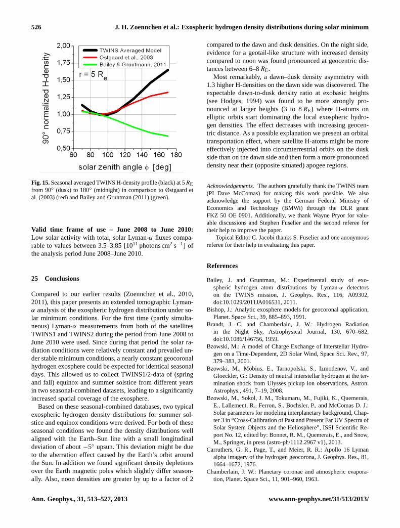
For a particular geocentric distance of 5RE we comparedour (ecliptic) H-densities for solar zenith anglesφ between90◦ (dusk) and 180◦ (midnight) with the solar zenith an-gle profiles published by Østgaard et al. (2003) and calcu-lated from the model published by Bailey and Gruntman(2011) (see Fig. 15). The H-density was normalized to 1 atφ = 90◦. Our seasonal-averaged model profile and the profileby Østgaard et al. (2003) both increase from dusk to midnightin a similar way. The solar zenith profile calculated from themodel by Bailey and Gruntman (2011) shows, however, a dif-ferent behavior with a H-density decrease from 90◦ to 180◦.

24 Range of validity (distance, solar activity, time)

Valid distances – from geocentric distance between3–8RE: The fits were done using TWINS1/2 LAD lines ofsight with geocentric intersection distances larger than 3REin order to be able to use the optically thin approximation.A Chamberlain-like density model for the lower regions,as described in Sect. 15, was used to present an adapted(spheric symmetric) model extension for lower altituderegions down to 1000 km.

Valid solar conditions – quiet, solar minimum conditions(F10.7cm < 100):The fits were done using data from the solarminimum with solar radio fluxes F10.7cm< 100 betweensummer solstice 2008 and summer solstice 2010 and shouldbe used only in situations with comparably low solar activity.



Fig. 15.Seasonal averaged TWINS H-density profile (black) at 5REfrom 90◦ (dusk) to 180◦ (midnight) in comparison to Østgaard etal. (2003) (red) and Bailey and Gruntman (2011) (green).

Valid time frame of use – June 2008 to June 2010:Low solar activity with total, solar Lyman-α fluxes compa-rable to values between 3.5–3.85 [1011 photons cm2 s−1] ofthe analysis period June 2008–June 2010.

25 Conclusions

Compared to our earlier results (Zoennchen et al., 2010,2011), this paper presents an extended tomographic Lyman-α analysis of the exospheric hydrogen distribution under so-lar minimum conditions. For the first time (partly simulta-neous) Lyman-α measurements from both of the satellitesTWINS1 and TWINS2 during the period from June 2008 toJune 2010 were used. Since during that period the solar ra-diation conditions were relatively constant and prevailed un-der stable minimum conditions, a nearly constant geocoronalhydrogen exosphere could be expected for identical seasonaldays. This allowed us to collect TWINS1/2-data of (springand fall) equinox and summer solstice from different yearsin two seasonal-combined datasets, leading to a significantlyincreased spatial coverage of the exosphere.

Based on these seasonal-combined databases, two typicalexospheric hydrogen density distributions for summer sol-stice and equinox conditions were derived. For both of theseseasonal conditions we found the density distributions wellaligned with the Earth–Sun line with a small longitudinaldeviation of about−5◦ upsun. This deviation might be dueto the aberration effect caused by the Earth’s orbit aroundthe Sun. In addition we found significant density depletionsover the Earth magnetic poles which slightly differ season-ally. Also, noon densities are greater by up to a factor of 2

compared to the dawn and dusk densities. On the night side,evidence for a geotail-like structure with increased densitycompared to noon was found pronounced at geocentric dis-tances between 6–8RE.

Most remarkably, a dawn–dusk density asymmetry with1.3 higher H-densities on the dawn side was discovered. Theexpectable dawn-to-dusk density ratio at exobasic heights(see Hodges, 1994) was found to be more strongly pro-nounced at larger heights (3 to 8RE) where H-atoms onelliptic orbits start dominating the local exospheric hydro-gen densities. The effect decreases with increasing geocen-tric distance. As a possible explanation we present an orbitaltransportation effect, where satellite H-atoms might be moreeffectively injected into circumterrestrial orbits on the duskside than on the dawn side and then form a more pronounceddensity near their (opposite situated) apogee regions.

Acknowledgements.The authors gratefully thank the TWINS team(PI Dave McComas) for making this work possible. We alsoacknowledge the support by the German Federal Ministry ofEconomics and Technology (BMWi) through the DLR grantFKZ 50 OE 0901. Additionally, we thank Wayne Pryor for valu-able discussions and Stephen Fuselier and the second referee fortheir help to improve the paper.

Topical Editor C. Jacobi thanks S. Fuselier and one anonymousreferee for their help in evaluating this paper.

References

Bailey, J. and Gruntman, M.: Experimental study of exo-spheric hydrogen atom distributions by Lyman-α detectorson the TWINS mission, J. Geophys. Res., 116, A09302,doi:10.1029/2011JA016531, 2011.

Bishop, J.: Analytic exosphere models for geocoronal application,Planet. Space Sci., 39, 885–893, 1991.

Brandt, J. C. and Chamberlain, J. W.: Hydrogen Radiationin the Night Sky, Astrophysical Journal, 130, 670–682,doi:10.1086/146756, 1959.

Bzowski, M.: A model of Charge Exchange of Interstellar Hydro-gen on a Time-Dependent, 2D Solar Wind, Space Sci. Rev., 97,379–383, 2001.

Bzowski, M., Mobius, E., Tarnopolski, S., Izmodenov, V., andGloeckler, G.: Density of neutral interstellar hydrogen at the ter-mination shock from Ulysses pickup ion observations, Astron.Astrophys., 491, 7–19, 2008.

Bzowski, M., Sokol, J. M., Tokumaru, M., Fujiki, K., Quemerais,E., Lallement, R., Ferron, S., Bochsler, P., and McComas D. J.:Solar parameters for modeling interplanetary background, Chap-ter 3 in “Cross-Calibration of Past and Present Far UV Spectra ofSolar System Objects and the Heliosphere”, ISSI Scientific Re-port No. 12, edited by: Bonnet, R. M., Quemerais, E., and Snow,M., Springer, in press (astro-ph/1112.2967 v1), 2013.

Carruthers, G. R., Page, T., and Meier, R. R.: Apollo 16 Lymanalpha imagery of the hydrogen geocorona, J. Geophys. Res., 81,1664–1672, 1976.

Chamberlain, J. W.: Planetary coronae and atmospheric evapora-tion, Planet. Space Sci., 11, 901–960, 1963.


http://dx.doi.org/10.1029/2011JA016531

http://dx.doi.org/10.1086/146756


Costa, J., Lallement, R., Quemerais, E., Bertaux, J. L., Kyrola, E.,and Schmidt, W.: Heliospheric interstellar H temperature fromSOHO/SWAN H cell data, Astron. Astrophys., 349, 660–672,1999.

Emerich, C., Lemaire, P., Vial, J.-C., Curdt, W., Schuhle, U., andWilhelm, K.: A new relation between the central spectral so-lar H I Lyman a irradiance and the line irradiance measuredby SUMER/SOHO during the cycle 23, Icarus, 178, 429–433,doi:10.1016/j.icarus.2005.05.002, 2005.

Fahr, H. J.: The Interplanetary Hydrogen Cone and its Solar CycleVariations, Astron. Astrophys., 14, 263–274, 1971.

Fahr, H. J. and Shizgal, B.: Modern Exospheric Theories and TheirObservational Relevance, Rev. Geophys. Space Phys., 21, 75–124, 1983.

Fuselier, S. A., Funsten, H. O., Heirtzler, D., Janzen, P., Kucharek,H., McComas, D. J., Moebius, E., Moore, T. E., Petrinec,S. M., Reisenfeld, D. B., Schwadron, N. A., Trattner, K.J., and Wurz, P.: Energetic neutral atoms from the Earth’ssubsolar magnetopause, Geophys. Res. Lett., 37, L13101,doi:10.1029/2010GL044140, 2010.

Hodges Jr., R. R.: Monte Carlo simulation of the terrestrial hydro-gen exosphere, J. Geophys. Res., 99, 23229–23247, 1994.

Johnson, F. S.: The Distribution of Hydrogen in the Telluric Hydro-gen Corona, Astrophys. Journal, 133, 701, 1961.

Kupperian, J. E., Byram, E. T., Chubb, T. A., and Friedman, H.:Far ultra-violet radiation in the night sky, Planet. Space Sci., 13,doi:10.1016/0032-0633(59)90015-7, 1959.

Lallement, R., Quemerais, E., Bertaux, J. L., Ferron, S.,Koutroumpa, D., and Pellinen, R.: Deflection of the InterstellarNeutral Hydrogen Flow Across the Heliospheric Interface, Sci-ence, 307, 1447–1449, 2005.

McComas, D. J., Allegrini, F., Baldonado, J., Blake, B., Brandt, P.C., Burch, J., Clemmons, J., Crain, W., Delapp, D., Demajistre,R., Everett, D., Fahr, H., Friesen, L., Funsten, H., Goldstein, J.,Gruntman, M., Harbaugh, R., Harper, R., Henkel, H., Holmlund,C., Lay, G., Mabry, D., Mitchell, D., Nass, U., Pollock, C., Pope,S., Reno, M., Ritzau, S., Roelof, E., Scime, E., Sivjee, M., Sk-oug, R., Sotirelis, T. S., Thomsen, M., Urdiales, C., Valek, P.,Viherkanto, K., Weidner, S., Ylikorpi, T., Young, M., and Zoen-nchen, J.: The two wide-angle imaging neutral-atom spectrom-eters (TWINS)NASA mission-of- opportunity, Space Sci. Rev.,142, 157,doi:10.1007/s11214-008-9467-4, 2009.

Mierkiewicz, E. J., Roesler, F. L., and Nossal, S. M.: Observed sea-sonal variations in exospheric effective temperatures, J. Geophys.Res., 117, A06313,doi:10.1029/2011JA017123, 2012.

Nass, H. U., Zoennchen, J. H., Lay, G., and Fahr, H. J.: The TWINS-LAD mission: Observations of terrestrial Lyman-? fluxes, Astro-phys. Space Sci. Trans., 2, 27–31,doi:10.5194/astra-2-27-2006,2006.

Østgaard, N., Mende, S. B., Frey, H. U., Gladstone, G. R., andLauche, H.: Neutral hydrogen density profiles derived from geo-coronal imaging, J. Geophys. Res. Space Phys., 108, 18-1, 2003.

Rairden, R. L., Frank, L. A., and Craven, J. D.: Geocoronal imagingwith Dynamics Explorer, J. Geophys. Res., 91, 13613–13630,1986.

Richter, E., Fahr, H. J., and Nass, H. U.: Satellite particle exospheresof planets – Application to earth, Planet. Space Sci., 27, 1163–1173,doi:10.1016/0032-0633(79)90136-3, 1979.

Sokol, J. M., Bzowski, M., Tokumaru, M., Fujiki, K., and McCo-mas, D. J.: Heliolatitude and Time Variations of Solar WindStructure from in situ Measurements and Interplanetary Scin-tillation Observations, Solar Physics, Online First, 05/2012,doi:10.1007/s11207-012-9993-9, 2012.

Thomas, G. E.: The interstellar wind and its influence on the inter-planetary environment, Annual review of earth and planetary sci-ences, 6, (A78-38764 16-42) Palo Alto, Calif., Annual Reviews,Inc., 1978, 173–204, 1978.

Thomas, G. E. and Bohlin, R. C.: Lyman-alpha measurements ofneutral hydrogen in the outer geocorona and in interplanetaryspace, J. Geophys. Res., 77, 2752–2761, 1972.

Witt, N., Blum, P. W., and Ajello, J. M.: Solar wind latitudinal vari-ations deduced from Mariner 10 interplanetary H /1216 A/ ob-servations, Astron. Astrophys., 73, 272–281, 1979.

Woods, T. N., Tobiska, W. K., Rottman, G. J., and Worden, J. R.:Improved solar Lyman alpha irradiance modeling from 1947through 1999 based on UARS observations, J. Geophys. Res.,105, 27195–27215,doi:10.1029/2000JA000051, 2000.

Zoennchen, J. H.: Modellierung der dreidimensionalen Dichte-verteilung des geokoronalen Neutralwasserstoffes auf Ba-sis von TWINS Ly-Alpha-Intensitaetsmessungen, Phd thesis,URN: urn:nbn:de:hbz:5N-08886, available at:http://www.ulb.uni-bonn.de/, 2006.

Zoennchen, J. H., Nass, U., Lay, G., and Fahr, H. J.: 3-D-geocoronalhydrogen density derived from TWINS Ly-?-data, Ann. Geo-phys., 28, 1221–1228,doi:10.5194/angeo-28-1221-2010, 2010.

Zoennchen, J. H., Bailey, J. J., Nass, U., Gruntman, M., Fahr, H.J., and Goldstein, J.: The TWINS exospheric neutral H-densitydistribution under solar minimum conditions, Ann. Geophys., 29,2211–2217,doi:10.5194/angeo-29-2211-2011, 2011.


http://dx.doi.org/10.1016/j.icarus.2005.05.002

http://dx.doi.org/10.1029/2010GL044140

http://dx.doi.org/10.1016/0032-0633(59)90015-7

http://dx.doi.org/10.1007/s11214-008-9467-4

http://dx.doi.org/10.1029/2011JA017123

http://dx.doi.org/10.5194/astra-2-27-2006

http://dx.doi.org/10.1016/0032-0633(79)90136-3

http://dx.doi.org/10.1007/s11207-012-9993-9

http://dx.doi.org/10.1029/2000JA000051

http://www.ulb.uni-bonn.de/

http://www.ulb.uni-bonn.de/

http://dx.doi.org/10.5194/angeo-28-1221-2010

http://dx.doi.org/10.5194/angeo-29-2211-2011

Documents

Exospheric hydrogen density distributions for equinox … · The aim of this analysis was the determination of two separate exospheric hydrogen models for equinox and ... sons summer