Expenditure Elasticities of the Demand for Leisure …college.holycross.edu/RePEc/spe/PawlowskiBreuer_Leisure...Working Paper Series, Paper No. 10-04 Expenditure Elasticities of the

Working Paper Series, Paper No. 10-04

Expenditure Elasticities of the Demand for Leisure Services

Tim Pawlowski† and Christoph Pawlowski

††

October 2010

Abstract

Although some research has already focused on the analysis of expenditure elasticities of

leisure demand, some shortcomings with regard to the content and the underlying theoretical

model as well as the applied methods exist. This paper aims at avoiding these problems to

provide consistent derivatives of leisure service expenditure elasticities. Therefore, a regular

demand system is derived from microeconomic duality theory. To implement leisure specific

demand factors (i.e., demand- and supply-based sports and recreational opportunities as well as

sports and recreational preferences) while still being consistent with neoclassical demand theory,

the basic model is extended by applying the demographic translation framework. Data of the

continuous household budget survey (n=7,724) from Germany is used for the estimation of the

derived demand system. It is shown how sensitive the results are depending on the applied

(censored) regression model: 16 out of 18 analyzed services are indicated as luxury goods based

on the findings of the Tobit model type I but as necessities based on the findings of the Tobit

model type II. Possible implications are presented and discussed.

JEL Classification Codes: D01, D12, L83

Key Words: Expenditure elasticity, demand, services, Tobit, Almost Ideal Demand System

† Institute of Sport Economics and Sport Management, German Sport University

Cologne, Institutsgebäude II, EG, Raum 5, Am Sportpark Müngersdorf 6 50933 Cologne,

Germany, Phone: +49-221-4982-6098, Fax: +49-221-4982-8141, [email protected] ††

Institute of Sport Economics and Sport Management, German Sport University

Cologne Institutsgebäude II, EG, Raum 5, Am Sportpark Müngersdorf 6 50933 Cologne,

Germany, Phone: +49-221-4982-6095, Fax: +49-221-4982-8144, [email protected]

mailto:[email protected]

1

INTRODUCTION

Demand elasticities are non-dimensional measures that indicate the sensitivity of

demand to variations in a particular economic and non-economic factor (Downward, Dawson,

and Dejonghe, 2008; Jones, 2004). Knowledge of the values of certain elasticities is of great

importance to management since they can inform strategic and operational marketing

decisions (Samuelson and Nordhaus, 2001). Amongst others, the price (Lindberg and

Aylward, 1999), the cross price (Henningsen, 2006), and the income or expenditure elasticities

(Salvatore, 2005) are the most significant elasticities in applied demand analysis. The latter

serves as a categorization tool for products and services in luxuries or necessities. Based on

this categorization, one might distinguish between growing and declining branches of products

and services in the future (Gratton and Taylor, 1992).

Although some research has already focused on the analysis of income or expenditure

elasticities for leisure demand, two major shortcomings exist: first, the studies are based on

highly aggregated data with few management implications and the risk of ecological fallacies;

second, many studies do not consider the censored sample problem in the context of demand

analysis, which is important especially in the case of sport because lack of participation can be

linked to zero expenditures. This paper aims at avoiding these shortcomings to provide

consistent derivatives of leisure service expenditure elasticities. Two main contributions are

offered, therefore.

First, to derive expenditure elasticities for a total of 18 leisure service categories based

on a consistent theoretical demand model; second, to show how sensitive the results are

depending on the applied (censored) regression model.

2

The paper is structured as follows: first, there is a presentation of the state of research on the

analysis of income effects on leisure service expenditure; second, we derive a comprehensive

theoretical model for the demand analysis of leisure services; third, we move on to the

definition of the data used in the current research and discuss the suitable methods and models

to overcome the sample selection problem; fourth, there is a presentation of the results.

Finally, the paper concludes with a discussion of the results and some ideas regarding further

research directions.

LITERATURE REVIEW

There is a substantial literature that examines the expenditure elasticities in the leisure

and tourism sectors. Blaine and Mohammad (1991) identify that the budget share for

recreation-related goods and services increases with an increasing total outlay. Therefore, the

recreation is indicated to be a luxury good (ε = 1.44). While the findings of an income elastic

demand for this broad category is in line with the findings of Martin and Mason (1980),

Moehrle (1990), Nelson (2001) and Sobel (1983), the latter detected product-related

differences: following Sobel (1983), products of the category “visible success” (e.g. vacation

expenditure, membership fees for clubs and organizations etc.) are luxuries (ε > 1) while

products of the category “home life” (e.g. expenditure on television, camping, and health and

sports equipment) are necessities (0 < ε < 1). Furthermore, Nelson (2001) identified that the

demand for “live events” is income inelastic (0 < ε < 1), and the Department of the Arts, Sport,

the Environment, Tourism and Territories (1988), identified differences in the income

elasticities between the households of different socioeconomic groups. Households with the

3

head of household working as a miner (ε = 1.73) as well as households with three or more

children (ε = 1.11) have an income elastic demand for sports and recreational products while

households with the head of household working in the service sector (ε = .82) as well as

households with only one child (ε = .94) show an income inelastic demand for the same

products. Dardis, Soberon-Ferrer, and Patro (1994) examined the impact of different income

components on the consumption expenditure on different goods. Even though they could

detect that all the significant effects are positive, some category-specific differences exist: the

salary of the head of household has only a significant impact on the consumption expenditure

for “passive leisure” (e.g. expenditure on products and services for television, radio, and

music) as well as “entertainment” (e.g. entrance fees for sport events, theaters, or museums).

In contrast, the salary of the marriage partner has only a significant impact on the consumption

expenditure on “active leisure” (e.g. expenditure on sports, fishing, or photography) while

other income components have a significant impact on all three expenditure categories.

Further, Blundell, Browning, and Meghir (1994) identified that services are luxuries (ε

= 2.11) in general, Gundlach (1993) found out that this holds true only for cross-section data.

His analysis of time series data reveals that the broad category containing all services tends to

be a necessity. Concerning tourism, Papanikos and Sakellariou (1997) found country-specific

differences, such that the Japanese demand for services is inelastic for outgoing tourism to the

Philippines (ε = .68), it is elastic for outgoing tourism to Malaysia (ε = 1.19). In a meta

analysis of tourism demand, Crouch detected a greater spread in the income elasticities for

general tourism demand ranging from ε = .28 (outgoing tourism to Latin America) to ε = 4.45

(outgoing tourism to developing countries in Asia). Cai, Hong, and Morrison (1995),

identified a significant positive relationship between income and the expenditure on

4

entertainment, sport events, museums, and tours, whilst Paulin (1990) detected an increasing

expenditure share for entertainment services on travelling. This is confirmed by Pyo, Uysal,

and McLellan (1991).

In summary, income is the most often analyzed demand factor. With few exceptions

(Legohérel and Hong, 2006; Leones, Colby, and Crandall, 1998; van Ophem and Hoog, 1994),

all the studies confirm a significant positive relationship between income and expenditure,

which means that the expenditure elasticities for the analyzed services are positive.

Nevertheless, it remains ambiguous whether the portion of leisure expenditure in relation to

the total outlay is decreasing indicating necessity goods (Euler, 1990, 0 < ε < 1), constant (Loy

and Rudman, 1983, ε = 1), or increasing indicating luxury goods (Wagner and Washington,

1982, ε > 1).

THEORETICAL MODEL

Neoclassical demand theory shows that the demand for goods and services by a household can

be derived either from utility maximization (the primal approach) or cost minimization (the

dual approach).

Following the primal approach the behavior of a household is rational if the perceived

utility of a bundle of goods and services is at least as high as the perceived utility of any of the

other bundles of goods and services available with the household‟s budget. Therefore, the

ideal consumption plan and, respectively, the household‟s demand functions for certain goods

and services can be derived from utility maximization subject to the household‟s budget

constraint with the Lagrange approach (see figure 1).

5

Insert figure 1 about here

Alternatively in the dual approach the behavior of a household is also rational if the

household selects goods to minimize the outlay in order to reach a certain utility level. In this

case, the ideal consumption plan and, respectively, the household‟s demand functions for a

bundle of certain goods and services can be derived from cost minimizing subject to a certain

utility level with the Lagrange approach. The possibility of backward calculation is of

particular interest for general demand analyses: Hicksian demand functions can be derived

from the cost function and Marshallian demand functions can be derived from the indirect

utility function (Deaton and Muellbauer, 1999). Such a system of demand functions

automatically satisfies the general restrictions of demand theory (homogeneity, adding up,

symmetry, non-negativity) and is called a regular demand system (Phlips, 1983). With the

Linear Expenditure System (LES), it was possible to estimate a regular demand system for the

first time (Geary, 1950–1951; Klein and Rubin, 1947–1948; Stone, 1954). However, the LES

is based on some restrictive assumptions: beside the additive utility function (which suggests

that the utility of a certain good only depends on the consumed quantity of this good and not

on any other good), the resulting constant income elasticities are extremely unrealistic (Deaton

and Muellbauer, 1999). In the course of time, new and more flexible demand systems were

developed and empirically verified. The most popular model that is based on a flexible cost

function is the Almost Ideal Demand System (AID System) by Deaton and Muellbauer (1980).

The numerous empirical estimations of the AID System, particularly in the recent past (Eakins

and Gallagher, 2003; Katchova and Chern, 2004; Matsuda, 2006), reflect the relevance of this

6

model to applied demand analyses. The starting point for the derivation of the AID System is a

specific cost function:

( ) ( )( ) a p Ub pc e (1)

The derivation and transformation of this specific form of the cost function leads to a system

of n equations, where the expenditure share of a good i ( iw ) is functionally linked to the prices

of other goods ( jp ), the own price as an index ( P ), and the income or total outlay (W ):

1

1 2n

i i i j j i

j

Ww ln p ln for each i , ,...,n

P (2)

In the current context two particularities lead to a modification of the original expenditure

share equations. The first is that because of data restrictions consumer behavior cannot be

analyzed with respect to the prices of goods. Given that prices are constant, the demand

system is reduced to a system of Engel curves. Therefore, the general restrictions related to the

price (homogeneity, symmetry, non-negativity) disappear. The single remaining general

restriction is the adding-up condition (Phlips, 1983). The AID System simplifies to (Missong,

2004):

1

1 2

i i i

n

i i i j i

j

w * ln W for each i , ,...,n

with * - (3)

Since the number of Engel curve parameters to be estimated ( *,i i) is smaller than the

number of Engel curve coefficients derived from the demand system ( , ,i i i j ), the

identification of the AID System is no longer possible. Nevertheless, the basic form known as

the Working–Leser Model (WLM: Leser, 1963; Working, 1943) also satisfies the adding-up

7

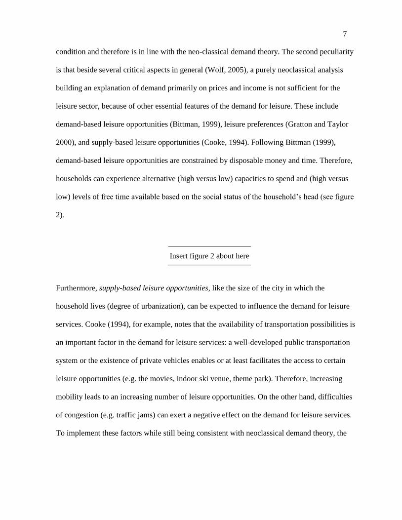
condition and therefore is in line with the neo-classical demand theory. The second peculiarity

is that beside several critical aspects in general (Wolf, 2005), a purely neoclassical analysis

building an explanation of demand primarily on prices and income is not sufficient for the

leisure sector, because of other essential features of the demand for leisure. These include

demand-based leisure opportunities (Bittman, 1999), leisure preferences (Gratton and Taylor

2000), and supply-based leisure opportunities (Cooke, 1994). Following Bittman (1999),

demand-based leisure opportunities are constrained by disposable money and time. Therefore,

households can experience alternative (high versus low) capacities to spend and (high versus

low) levels of free time available based on the social status of the household‟s head (see figure

2).


Furthermore, supply-based leisure opportunities, like the size of the city in which the

household lives (degree of urbanization), can be expected to influence the demand for leisure

services. Cooke (1994), for example, notes that the availability of transportation possibilities is

an important factor in the demand for leisure services: a well-developed public transportation

system or the existence of private vehicles enables or at least facilitates the access to certain

leisure opportunities (e.g. the movies, indoor ski venue, theme park). Therefore, increasing

mobility leads to an increasing number of leisure opportunities. On the other hand, difficulties

of congestion (e.g. traffic jams) can exert a negative effect on the demand for leisure services.

To implement these factors while still being consistent with neoclassical demand theory, the

8

Working–Leser Model is extended by integrating the demographic translation framework

(Pollak and Wales, 1992) with leisure-specific factors:

0

1

1 2s

i i ir r i

r

w q q t b ln W for each i , ,...,n (4)

From a theoretical point of view, this functional form assumes that the additional factors, like

the degree of urbanization (rt ), have an impact on the constant term. In contrast, the sensitivity

of the demand response to changes in the disposable income does not depend on the extent of

these factors.

To derive the service-specific expenditure elasticities, the expenditure share equations have to

be transformed into demand functions by multiplying with the total outlay (W ) (Blaas and

Sieber, 2000).

0

1

1 2s

i i i ir r i

r

e Ww W t ln W for each i , ,...,n (5)

The expenditure elasticities indicate the percentage change in the expenditure for a certain

leisure service that will follow any given percentage change in the total outlay. Therefore,

expenditure elasticities are the product of the first-order derivative and the quotient of total

outlay to the expenditure for a certain leisure service:

,

( )* 1,2,...,

i

ie W

i

e W Wfor each i n

W e (6)

For Working–Leser demand functions, this is:

0

1

1 11 2

i

s

e ,W i ir r i i

r i

e q q t b ln W bW * for each i , ,...,nW w

(7)

or

9

0

1

11 2

i

s

e ,W i ir r i i

r i

t ln W * for each i , ,...,nw

(8)

or

11 2

ie ,W i i

i

w * for each i , ,...,nw

(9)

or

, 1 1,2,..., i

ie W

i

for each i nw

(10)

While the sensitivity of the demand response to changes in the disposable income does not

depend on the extent of sociodemographic factors directly though, of course, in estimating βi it

depends on the certain budget share (iw ). Therefore, it is possible to derive demographically

scaled expenditure elasticities based on household-specific budget shares that might serve as

an indicator of household-specific consumption patterns (Brosig, 2000). Furthermore, the

value of the expenditure elasticities depends on the calculated coefficient of the logarithmized

total outlay (i).

METHOD

Following equation (10), to derive the category-dependent expenditure elasticities, the

expenditure shares (iw ) have to be calculated and the coefficients of the logarithmized total

outlay (i) have to be estimated. The methodological framework to derive the latter is

described in the following chapters in detail.

10

Data and Estimator

To derive the expenditure category-dependent elasticities, data from the continuous household

budget survey (CHBS) from 2006 (n=7,724) is used. Since 2005, the CHBS as the quota

sample has been based on the representative sample of the survey of household income and

expenditure (SHIE). The characteristics used to select the households are: the type of

household, the employment status of the head of household (yes/no), and the income class of

the head of household. The sample of the CHBS data is extrapolated to the complete country

(in analogy to the extrapolation of the SHIE data) by applying a specific extrapolation factor

(Fleck and Papastefanou 2006).

In this study, we analyse a total number of 18 different leisure services from 3 different

aggregation levels: beside the broadest category (leisure services: LEISURE), which is made

up of the sports and recreational services (SPORT) as well as the cultural services

(CULTURE), we have access to data for the following subcategories: sport event admission

(EVENT), entrance fees for swimming pools (POOL), music lessons (MUSIC), dancing

lessons (DANCE), fitness center fees (FITNESS), ski lift fees (SKI), sport club membership

fees (CLUB), opera admission (OPERA), theater admission (THEATER), cinema admission

(CINEMA), circus admission (CIRCUS), museum admission (MUSEUM), zoo admission

(ZOO), fees for pay TV (PAYTV) and the rental of video films (FILM).

Although this study focuses on expenditure elasticities and therefore primarily on the

relationship between (logarithmized) total outlay and budget shares, that is, the estimation of

i, it is always desirable to estimate a complete model with all the factors that are supposed to

influence the consumption expenditure (Backhaus et al., 2003). In order to take leisure-

11

specific demand factors into account, the degree of urbanization (fewer than 20,000

inhabitants, 20,000–99,999 inhabitants, 100,000 and more inhabitants) and the area

(northwest, northeast, south) where the household is located are included in the model.

Furthermore, the reported quarter (January–March, April–June, July–September, October–

December) and the age, the social status (public official, white-collar worker, blue-collar

worker, unemployed person, retired person, student), the level of education (high-school

diploma and higher), and the marital status (married, single) of the head of the household, as

well as the structure of the household (children aged 6 years and under, children aged 6–18

years, children aged 18 years and above, number of people in the household) are included in

the model.

Summing up, the expenditure shares of the m leisure services serve as dependent variables

and, along with the logarithmized total household expenditure and the leisure-specific factors

as independent variables, make up a system of m regression equations. As discussed below, a

number of possible estimators can be used to analyse the data.

Tobit Model Type I

Since not all the households spent their income on all the leisure service items, numerous zero

observations exist in the data and we are faced with the so-called censored sample problem.

The censored sample problem is one of the most discussed problems in applied demand

analysis and is mostly related to expenditure analysis (Barslund, 2007; Czarnitzki and

Stadtmann,2002; Dardis et al., 1994; Deaton and Muellbauer, 1999; Lera-Lopéz and Rapún-

Gárate, 2005; Lin, 2006; Long, 1997; Phlips, 1983; Shonkwiler and Yen, 1999; Thrane, 2001;

12

Wooldridge, 2003). To avoid biased estimates (Pawlowski et al., 2009), the basic model has to

be modified.

With his econometric study of durable goods, Tobin (1958) was the first to develop a modified

concept of analyzing consumer demand and solving the censored sample problem. Following

Tobin‟s approach (Tobit model type I; Amemiya, 1985), it is assumed that a latent variable

that measures the consumer‟s propensity to spend money on a certain leisure service ( *

hw ) is in

linear relation to a vector of influencing variables (hZ ) and undetectable influences (

h):

*

h h hw Z (11)

It is assumed that a household h spends ( *

hw ) on a certain leisure service if the latent variable

( *

hw ) is positive. In contrast to the observed expenditure share of households h ( hw ), the value

of the unobservable variable ( *

hw ) can be negative. For negative values of the latent variable,

the household will not spend any money on the leisure service:

* *

*

0

0 0

h h

h

h

w if ww

if w (12)

In the next step, the likelihood function can be developed, which consists of two parts (Franz,

2006): the product of the probabilities that households do not spend any money on the certain

leisure service [ 0hPr ( w )] and the product of the probabilities that households spend

( *

hw ) on the leisure service [*

h hPr ( w w ) ]:

0 *

e h h h

censored uncensored

L( , ) Pr( w ) Pr( w w ) (13)

13

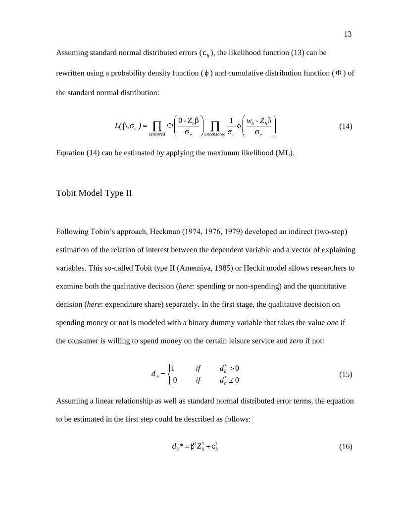
Assuming standard normal distributed errors (h), the likelihood function (13) can be

rewritten using a probability density function ( ) and cumulative distribution function ( ) of

the standard normal distribution:

0 1h h he

censored uncensorede e e

- Z w - ZL( , ) (14)

Equation (14) can be estimated by applying the maximum likelihood (ML).

Tobit Model Type II

Following Tobin‟s approach, Heckman (1974, 1976, 1979) developed an indirect (two-step)

estimation of the relation of interest between the dependent variable and a vector of explaining

variables. This so-called Tobit type II (Amemiya, 1985) or Heckit model allows researchers to

examine both the qualitative decision (here: spending or non-spending) and the quantitative

decision (here: expenditure share) separately. In the first stage, the qualitative decision on

spending money or not is modeled with a binary dummy variable that takes the value one if

the consumer is willing to spend money on the certain leisure service and zero if not:

*

*

1 0

0 0

h

h

h

if dd

if d (15)

Assuming a linear relationship as well as standard normal distributed error terms, the equation

to be estimated in the first step could be described as follows:

1 1 1*h h hd Z (16)

14

In the second stage, we could detect a positive value of the expenditure share (hw ) if the

money-spending decision in the first stage is positive:

* *

*

0

0 0

h h

h

h

w if dw

if d (17)

Again, under simplifying assumptions (linear relationship, standard normal distributed error

terms), the equation to be estimated in the second stage could be described as follows (note

that it is not necessary for 1

hZ to equal 2

hZ ):

* 2 2 2

h h hw Z (18)

If ( 1

h ) and ( 2

h ) are correlated, ordinary least squares (OLS) estimation based only on

uncensored observations would yield biased estimates ( 2 ) since the conditional expected

value of the error term [ 2 1 1 1( ³ - )h h hE Z ] is neglected:

2 2 2 2 1 1 1( , 1) ( ³ - )h h h h h h hE w Z d Z E Z (19)

Assuming standard normal distributed errors, equation (19) can be rewritten using a

probability density function ( ) and a cumulative distribution function ( ) of the standard

normal distribution as well as a standard deviation of errors ( ) and correlation of errors ( )

as follows:

1

1

1 1

2 2 2

1 1

( )( , 1)

( )

h

h h h h h

h

ZE w Z d Z with

Z (20)

By applying the two-step estimation procedure, it is possible to specify consistent estimators

( ): (1) in a first step, the probit model is estimated by applying the ML to all observations.

15

The resultant estimators are used to calculate (h

), which is known as the hazard rate or

inverse Mill‟s ratio (IMR). (2) By applying OLS estimation only to uncensored observations

in a second step, all the parameters ( 2 ) can be estimated since all the individual hazard rates

can be implemented as ordinary explanatory variables (note that the estimated coefficient ( )

represents the product of ( 2 1 2 )).

Model Selection

Contrary to Tobin‟s approach, with the separate estimation of the qualitative and the

quantitative equations, the coefficients in the Tobit model type II are not constrained to be the

same sign for both decisions (Weagley and Huh, 2004). Furthermore, zero observations do not

have to be the result of corner solutions, which means that a sufficiently large change in

explanatory variables would ultimately create a positive consumption expenditure for any

given household (Verbeek, 2005). In this case, the Tobit model type II appears more flexible

than the Tobit model type I. On the other hand, in contrast to the Tobit model type II, the

researcher does not have to specify a priori identifying variables (variables in the vector of 1

hZ

that do not belong to the vector of 2

hZ ) in the basic model by James Tobin. While no general

agreement or guidance concerning the selection of the identifying variables exists, it is a

crucial point and might heavily influence the estimation results (Verbeek, 2005). Therefore,

both models are faced with certain advantages and limitations so that it is not possible to state

a priori which one is best suited to this research context.

16

While other single equation models (e.g. the double hurdle model) do not appear to be more

appropriate from the theoretical point of view, it has to be discussed whether a multivariate

Tobit model might be necessary. Such models are required if the qualitative and/or the

quantitative decisions of a certain leisure service depend on the corresponding decisions

concerning other leisure services. From a statistical point of view, this is the case if the error

terms of two leisure services in the same stage are correlated. While this does not seem

unrealistic (e.g. a general preference factor for or against sport might exist that is not part of

the set of available independent variables), the development of adequate multivariate models

is not satisfying: an approach developed by Heien and Wessells (1990) is not consistent while

the model developed by Shonkwiler and Yen (1999) generates inefficient estimates

(Tauchmann, 2005). However, since Halvorsen and Nesbakken (2004) find that stochastic

interdependencies (e.g. a seemingly unrelated regression (SUR) in the second stage of the

Tobit model type II) does not yield appreciable different estimates, our analysis is focused on

the single equation approaches by Tobin and Heckman. To compare the results, we also

present the subsample OLS estimation without correction of the sample selection.

Applying the Tobit models types I and II, the estimated coefficients of total outlay (i) also

cover the effect of total outlay on the qualitative decision. Therefore, to derive the expenditure

elasticities, we use the marginal effects instead of the estimated coefficient (i) following the

approaches of McDonald and Moffitt (1980) for the Tobit model type I and of Hoffmann and

Kassouf (2005) for the Tobit model type II. For comparability reasons, the derived

expenditure elasticities are conditional to such households with expenditure in the

corresponding category.

17

RESULTS

With more than 25 billion euros, German households spent around 3% of their disposable

budget on leisure services in 2006. Of the analyzed subcategories, CLUB with around 3.2

billion euros, MUSIC with more than 1.3 billion euros, and FITNESS with around 1.2 billion

euros are the most significant ones. While nearly all of the participating households spent any

money on leisure services (97.3%), some subcategories exist where only a few households

spent money (e.g. PAYTV: 2.7%). Table 1 provides an overview of the annual leisure service

expenditure and the portion of households that spent in the corresponding category.

Insert table 1 about here

Regarding the goodness of fit of a Tobit model type I, various pseudo-R2 statistics can be

applied. Based on numerous Monte Carlo simulations, Veall and Zimmermann (1996) could

detect that the pseudo-R2 by McKelvey and Zavoina (1975) is best suited to a direct

comparison with the coefficient of determination (R2) of the OLS estimations for the Tobit

model type II and the linear model without correction of the sample selection. All in all, we

estimated 54 (three per expenditure category) different regression models that show rather

high variance explanatory power (values of R2 measure up to 52.47%). This indicates that the

set of selected determinants seems to be quite appropriate for explaining the German

households‟ expenditure patterns on leisure services.

18

Out of 54 coefficients, 46 show a highly significant impact of logarithmized total outlay on the

analyzed expenditure shares. Amongst others, table 2 summarizes the conditional marginal

effects that are based on these coefficients.


Interestingly, while the Tobit models type I indicate a significant positive impact of the

logarithmized total outlay on the budget share, the other models indicate a significant negative

one. This is the result of the contrary impact of logarithmized total outlay on the qualitative

and the quantitative consumer decision: as the first step probit estimation results of the Tobit

model type II verify, it appears that the logarithmized total outlay has a significant positive

impact on the probability of consuming leisure services for all categories. Therefore, while the

simultaneous Tobit models type I can only display the same sign for both decisions

(qualitative, quantitative), the Tobit models type II could reveal a highly significant category-

independent contrarian effect of logarithmized total outlay on the analyzed expenditure shares.

Following equation 10, we can derive the category-specific expenditure elasticities based on

the conditional marginal effects and the budget share. It is obvious that these model-specific

differences between the estimation results have a considerable impact on the derived

expenditure elasticities that are displayed on average for all households as well as for certain

socio-demographic subgroups of households in table 3.


19

Therefore, all the analyzed services (except LEISURE and CULTURE) are indicated as luxury

goods (ε > 1) based on the findings of the Tobit model type I but as necessities (0 < ε < 1)

based on the findings of the Tobit model type II and the linear model without correction of the

sample selection (see figure 3).


LIMITATIONS AND DIRECTIONS OF FURTHER RESEARCH

In the above-described sections, we could derive expenditure elasticities for three aggregated

categories and 15 subcategories of leisure services in Germany. The derivation is based on a

consistent theoretical demand model with necessary and suitable extensions to consider the

particularities in the field of leisure. Like many other studies on consumption expenditure, we

are faced with the censored sample problem. To avoid biased estimates and elasticities, we

applied different kinds of extended regression models. Obviously, we could see that the

resulting expenditure elasticities are highly sensitive to the applied (censored) regression

model. Due to the fact that Tobit models type I do not distinguish between the qualitative

decision (whether or not to consume) and the quantitative decision (how much to spend), the

resulting estimates are the same. This appears problematical, especially in the field of leisure

service research, since we could detect that the logarithmized total outlay has a highly

significant positive effect on the probability of consuming leisure services but a highly

significant negative effect on the allocated budget share for the certain expenditure category.

20

This leads to the striking question: which model is the right model? Due to the already-

discussed shortcomings of both models, it is not possible to present a first-best solution to this

problem. One possible selection criterion might be the goodness of model fit (see table 2).

Indeed, for most of the expenditure categories, we could detect significant differences

concerning the goodness of fit between the different model types. For five out of 18

expenditure categories (SPORT, MUSIC, SKI, MUSEUM, FILM), the Tobit model type I

indicates the best goodness of fit value while there is a significantly higher value for the Tobit

models type II for nine out of 18 expenditure categories (CULTURE, DANCE, FITNESS,

OPERA, THEATER, CINEMA, CIRCUS, ZOO, PAYTV). Only four out of 18 expenditure

categories (LEISURE, EVENT, POOL, CLUB) show a similar goodness of fit between the

three different models. Given these empirical results, care should be taken with model

selection and it seems at least advisable to estimate different model types and not jump to

conclusions.

It would be desirable for further research to test whether similar consumption patterns exist for

other services and in other countries. Furthermore, much effort should be put into the

development and empirical validation of modified models that consider the censored sample

problem in a reasonable way.

21

REFERENCES

Amemiya, T. (1985) Advanced Econometrics, Basil Blackwell, Oxford.

Backhaus, K., Erichson, B., Plinke, W. & Weiber R. (2006) Multivariate

Analysemethoden - eine anwendungsorientierte Einführung, Springer, Berlin.

Barslund, M. C. (2007) Estimation of Tobit Type Censored Demand Systems: A Comparison

of Estimators, Discussion Paper No. 07-16, Department of Economics, University of

Copenhagen, Denmark.

Bittman, M. (1999) Social Participation and Family Welfare: The Money and Time Costs of

Leisure, Discussion Paper No. 95, SPRC, Sydney.

Blaas, W. & Sieber, L. (2000) Schätzung von direkten Preis-, Kreuzpreis- und

Einkommenselastizitäten basierend auf einem vollständigen Konsummodell unter

besonderer Berücksichtigung des Marktes alkoholfreier Getränke, Working Paper No.

1/2000, Institut für Finanzwissenschaft und Infrastrukturpolitik, Technische Universität

Wien, Austria.

Blaine, T. W. & Mohammad, G. (1991) An Empirical Assessment of U.S. Consumer

Expenditures for Recreation-Related Goods and Services: 1946-1988, Leisure

Sciences, 13 (2), 111–22.

Blundell, R., Browning, M. & Meghir, C. (1994) Consumer Demand and the Life-Cycle

Allocation of Family Expenditures, Review of Economic Studies, 61 (206),

57–80.

22

Brosig, S. (2000) A Model of Household Type Specific Food Demand Behaviour in Hungary,

Discussion Paper No. 30, Institut für Agrarentwicklung in Mittel- und Osteuropa,

Halle.

Cai, L. A., Hong, G.-S. & Morrison, A. M. (1995) Household Expenditure Patterns for

Tourism Products and Services, Journal of Travel & Tourism Marketing, 4 (4), 15–40.

Czarnitzki, D. & Stadtmann, G. (2002) Uncertainty of Outcomes versus Reputation: Empirical

Evidence for the First German Football Division, Empirical Economics, 27 (1), 101–

12.

Cooke, A. (1994) The Economics of Leisure and Sport, Routledge, New York.

Crouch, G. I. (1995) A Meta-Analysis of Tourism Demand, Annals of Tourism Research, 22

(1), 103–18.

Dardis, R., Soberon-Ferrer, H. & Patro, D. (1994) Analysis of Leisure Expenditures in the

United States, Journal of Leisure Research, 26 (4), 309–36.

Deaton, A. & Muellbauer, J. (1980) An Almost Ideal Demand System, The American

Economic Review, 70 (3), 312–26.

––––– (1999) Economics of Consumer Behavior, University Press, Cambridge.

Department of the Arts, Sport, the Environment, Tourism and Territories (1988) The

Economic Impact of Sport and Recreation – Household Expenditure, Technical Paper

No. 1, Australian Government Publishing Service, Canberra.

Downward, P., Dawson, A. & Dejonghe, T. (2009) Sports Economics – Theory, Evidence and

Practice, Elsevier, Oxford.

23

Eakins, J. M. & Gallagher, L. A. (2003) Dynamic Almost Ideal Demand Systems: An

Empirical Analysis of Alcohol Expenditure in Ireland, Applied Economics, 35 (9),

1025–36.

Euler, M. (1990) Ausgaben privater Haushalte für Freizeitgüter, Wirtschaft und Statistik, 3,

219–27.

Fleck, M., & Papastefanou, G. (2006) Einkommens- und Verbrauchstichprobe 1998 – Design

und Methodik sowie Veränderungen gegenüber den Vorgängererhebungen,

Arbeitsbericht Nr. 2006/01, ZUMA, Mannheim.

Franz, W. (2006), Arbeitsmarktökonomik, Springer, Berlin.

Geary, R. C. (1950–1951) A Note on „A Constant Utility Index of the Cost of Living‟, Review

of Economic Studies, 18, 65–66.

Gratton, C. & Taylor, P. (1992) Economics of Leisure Services Management, 2nd

ed.,

Longman, Harlow.

Gratton, C. & Taylor, P. (2000) Economics of Sport and Recreation, Spon Press, London.

Gundlach, E. (1993) Die Dienstleistungsnachfrage als Determinante des wirtschaftlichen

Strukturwandels, Mohr, Tübingen.

Halvorsen, B. & Nesbakken, R. (2004) Accounting for Differences in Choice Opportunities in

Analyses of Energy Expenditure, Discussion Paper No. 400, Research Department,

Statistics Norway, Oslo.

Heckman, J. (1974) Shadow Prices, Market Wages and Labor Supply, Econometrica, 42 (4),

679–94.

24

––––– (1976) The Common Structure of Statistical Models of Truncation, Sample Selection

and Limited Dependent Variables and a Simple Estimator for Such Models, Annals of

Economic and Social Measurement, 5 (4), 475–92.

––––– (1979) Sample Selection Bias as a Specification Error, Econometrica, 47 (1), 153–61.

Heien, D. & Wessells, C. R. (1990) Demand System Estimation with Microdata: A Censored

Regression Approach, Journal of Business Economic Statistics, 8 (3), 365–71.

Henningsen, A. (2006) Modellierung von Angebots- und Nachfrageverhalten zur Analyse von

Agrarpolitiken: Theorie, Methoden und empirische Anwendungen, Agrar- und

Ernährungswissenschaftliche Fakultät, Christian-Albrechts-Universität, Kiel.

Hoffmann, R. & Kassouf, A. L. (2005) Deriving Conditional and Unconditional Marginal

Effects in Log Earnings Equations Estimated by Heckman‟s Procedure,

Applied Economics, 37 (11), 1303–311.

Jones, T. (2004), Business Economics and Managerial Decision Making, Wiley, Chichester.

Katchova, A. L. & Chern, W. S. (2004) Comparison of Quadratic Expenditure System and

Almost Ideal Demand System Based on Empirical Data, International Journal of

Applied Economics, 1 (1), 55–64.

Klein, L. R. & Rubin, H. (1947–1948) A Constant-Utility Index of the Cost of Living, Review

of Economic Studies, 15, 84–87.

Legohérel, P. & Hong, K. K. F. (2006) Market Segmentation in the Tourism Industry and

Consumers‟ Spending: What about Direct Expenditures? Journal of Travel and

Tourism Marketing, 20 (2), 15–30.

25

Leones, J., Colby, B. & Crandall, K. (1998) Tracking Expenditures of the Elusive Nature

Tourists of South-Eastern Arizona, Journal of Travel Research, 36 (3), 56–64.

Lera-López, F. & Rapún-Gárate, M. (2005) Sports Participation versus Consumer Expenditure

on Sport: Different Determinants and Strategies in Sport Management, European Sport

Management Quarterly, 5 (2), 167–86.

Leser, C. E. V. (1963) Forms of Engel Functions, Econometrica, 31 (4), 694–703.

Lin, B.-H. (2006), A Sample Selection Approach to Censored Demand Systems, American

Journal of Agricultural Economics, 88 (3), 742–49.

Lindberg, K. & Aylward, B. (1999) Price Responsiveness in the Developing Country Nature

Tourism Context: Review and Costa Rican Case Study, Journal of Leisure Research,

31 (3), 281–99.

Long, S. J. (1997) Regression Models for Categorical and Limited Dependent Variables,

Sage, Thousand Oaks.

Loy, J. W. & Rudman, W. J. (1983) Social Physics and Sport Involvement. An Analysis of

Sport Consumption and Production Patterns by Means of Three Empirical Laws, S.A.

Journal for Research in Sport, Physical Education and Recreation, 6 (2), 31–48.

Martin, W. H. & Mason, S. (1980) Broad Patterns of Leisure Expenditure, The Sports Council

and Social Science Research Council, London.

Matsuda, T. (2006) Linear Approximations to the Quadratic Almost Ideal Demand System,

Empirical Economics, 31 (3), 663–75.

McDonald, J. F. & R. A. Moffitt (1980) The Uses of Tobit Analysis, The Review of Economics

and Statistics, 62, 318–87.

26

McKelvey, R. & Zavoina, W. (1975) A Statistical Model for the Analysis of Ordinal Level

Dependent Variables, Journal of Mathematical Sociology, 4, 103–20.

Missong, M. (2004) Demographisch gegliederte Nachfragesysteme und Äquivalenzskalen für

Deutschland, Duncker & Humblot, Berlin.

Moehrle, T. (1990) Expenditure Patterns of the Elderly: Workers and Nonworkers, Monthly

Labor Review, 113 (May), 34–41.

Nelson, J. P. (2001) Hard at Play! The Growth of Recreation in Consumer Budgets, 1959-

1998, Eastern Economic Journal, 27 (1), 35–53.

Papanikos, G. T. & Sakellariou, C. (1997) An Econometric Application of the Almost Ideal

Demand System Model to Japan‟s Tourist Demand for ASEAN Destinations, Journal

of Applied Recreation Research, 22 (2), 157–72.

Paulin, G. (1990) Consumer Expenditures on Travel, 1980-87, Monthly Labor Review, 113

(6), 56–60.

Pawlowski, T., Breuer, C., Wicker, P. & Poupaux, S. (2009) Travel Time Spending Behavior

in Recreational Sports: An Econometric Approach with Management Implications,

European Sport Management Quarterly, 9 (3), 215–42.

Phlips, L. (1983) Applied Consumption Analysis, North-Holland, Amsterdam.

Pollak, R. A. & Wales, T. J. (1992) Demand System Specification and Estimation, University

Press, Oxford.

Pyo, S.-S., Uysal, M. & McLellan, R. W. (1991) A Linear Expenditure Model for Tourism

Demand, Annals of Tourism Research, 18 (3), 443–54.

27

Salvatore, D. (2005) Introduction to International Economics, John Wiley & Sons, Hoboken,

New Jersey.

Samuelson, P. A. & Nordhaus, W. D. (2001) Economics, McGraw-Hill, New York.

Shonkwiler, S. J. & Yen, S. T. (1999) Two-Step Estimation of a Censored System of

Equations, American Journal of Agricultural Economics, 81 (4), 972–82.

Sobel, M. E. (1983) Lifestyle Expenditures in Contemporary America, American Behavioral

Scientist, 26 (4), 521–33.

Stone, R. J. N. (1954) Linear Expenditure Systems and Demand Analysis: An Application to

the Pattern of British Demand, Economic Journal, 64, 511–27.

Tauchmann, H. (2005) Efficiency of Two-Step Estimators for Censored Systems of Equations:

Shonkwiler & Yen Reconsidered, Applied Economics, 37 (4), 367–74.

Thrane, C. (2001) Sport Spectatorship in Scandinavia. A Class Phenomenon? International

Review for the Sociology of Sport, 36 (2), 149–63.

Tobin, J. (1958) Estimation of Relationships for Limited Dependent Variables, Econometrica,

26 (1), 24–36.

Van Ophem, J. & de Hoog, K. (1994) Differences in Leisure Behaviour of the Poor and the

Rich in the Netherlands, in Leisure: Modernity, Postmodernity and Lifestyles, Vol. I,

(Ed.) I. Henry, The Leisure Studies Association, University of Brighton, pp. 291–305.

Veall, M. R. & Zimmermann, K. F. (1996) Pseudo-R2 Measures for Some Common Limited

Dependent Variable Models, Sonderforschungsbereich 386, Paper 18, LMU,

München.

28

Verbeek, M. (2005) A Guide to Modern Microeconometrics, 2nd

ed., Wiley, Chichester.

Wagner, F. & Washington, V. R. (1982) An Analysis of Personal Consumption Expenditures

as Related to Recreation, 1946-1976, Journal of Leisure Research, 14 (1), 37–46.

Weagley, R. O. & Huh, E. (2004) Leisure Expenditures of Retired and Near-Retired

Households, Journal of Leisure Research, 36 (1), 101–27.

Wolf, D. (2005) Ökonomische Sicht(en) auf das Handeln. Ein Vergleich der Akteursmodelle in

ausgewählten Rational-Choice- Konzeptionen, Metropolis, Marburg.

Wooldridge, J. M. (2003) Introductory Econometrics. A Modern Approach, 2nd

ed., Thomson

South-Western, Mason.

Working, H. (1943) Statistical Laws of Family Expenditure, Journal of the American

Statistical Association, 38 (221), 43–56.

29

TABLES

Table 1

Annual Leisure Service Expenditure (Source: CHBS, 2006; Own Calculations)

Households with leisure service expenditure

# Service

category

Number

Percentage

Total annual expenditure (million €)

a

Mean annual expenditure

(€)b

Mean budget

sharec

(1) LEISURE 7,513 97.3 25,100 312.0 3.105

(2) SPORT 5,362 69.4 11,100 255.5 1.832 (3) CULTURE 7,399 95.8 14,000 207.4 1.946

(4) EVENT 1,146 14.8 616 68.1 .510 (5) POOL 1,667 21.6 706 48.6 .406 (6) MUSIC 584 7.6 1,344 295.2 1.822 (7) DANCE 275 3.5 361 164.0 1.178 (8) FITNESS 643 8.3 1,279 253.3 2.118 (9) SKI 363 4.7 538 191.9 1.407 (10) CLUB 2,572 33.3 3,246 152.9 1.223

(11) OPERA 400 5.2 556 189.3 1.292 (12) THEATER 522 6.8 383 96.2 .680

(13) CINEMA 1,993 25.8 646 40.4 .330 (14) CIRCUS 199 2.6 121 61.1 .487

(15) MUSEUM 2,184 28.3 633 37.8 .280 (16) ZOO 754 9.8 254 42.1 .322 (17) PAYTV 205 2.7 271 170.1 1.455 (18) FILM 346 4.5 73 25.4 .203 a “Total” refers to the total expenditure in Germany in 2006.

b “Mean” refers to the per capita expenditure of households with expenditure greater than zero.

c “Mean” refers to the mean budget share of households with expenditure greater than zero.

30

Table 2

Goodness of Model Fit and Conditional Marginal Effects of Logarithmized Total Outlay

(Source: CHBS, 2006; Own Calculations)

Goodness of

model fita

Conditional marginal effect of logarithmized total outlay

b

# Service

category T I T II OLS

T I T II OLS

(1) LEISURE 5.90 5.43 5.30 -.0006759 -.0028992 -.0048814

(2) SPORT 15.50 6.75 6.75

.0035657 -.0041103 -.0038425 (3) CULTURE 6.70 10.65 10.62 -.0022585 -.0079035 -.0072907

(4) EVENT 10.70 9.45 9.25

.0006757 -.0005241 -.0005966 (5) POOL 11.10 11.63 11.62 .0003271 -.0028872 -.0028810 (6) MUSIC 28.40 15.18 13.69 .0008770 -.0117653 -.0087452 (7) DANCE 15.70 27.49 27.24 .0009183 -.0064142 -.0066614 (8) FITNESS 11.80 27.00 26.90 .0019654 -.0147181 -.0145038 (9) SKI 23.30 20.18 15.53 .0017869 -.0031143 -.0038634 (10) CLUB 10.20 10.12 10.12 .0015834 -.0065077 -.0065183

(11) OPERA 11.60 17.94 17.74

.0018995 -.0066436 -.0066001 (12) THEATER 10.50 16.32 14.42 .0008289 -.0019656 -.0016553 (13) CINEMA 17.30 20.14 20.10 .0003173 -.0023676 -.0023051 (14) CIRCUS 11.20 16.80 16.08 .0004309 -.0014026 -.0014058 (15) MUSEUM 11.20 6.98 6.73 .0005324 -.0011510 -.0012276 (16) ZOO 14.70 21.07 21.06 .0002648 -.0029747 -.0029648 (17) PAYTV 13.80 52.47 51.85 .0008341 -.0086996 -.0091136 (18) FILM 27.80 15.66 14.85 .0001546 -.0012159 -.0012974 a “Goodness of model fit” refers to the pseudo-R

2 by McKelvey and Zavoina

(1975) for the Tobit model type I and the coefficient of determination (R2) for

the Tobit model type II and the linear model without correction of the sample selection. b “Conditional marginal effect of logarithmized total outlay” refers to the

estimated coefficient of the logarithmized total outlay for the linear model without correction of the sample selection and the transformed coefficient for the Tobit models type I (McDonald and Moffitt 1980) and II (Hoffmann and Kassouf 2005). T I ≡ Tobit model type I, T II ≡ Tobit model type II, OLS ≡ linear model without correction of the sample selection.

31

Table 3

Demographical Scaled Expenditure Elasticities (Source: CHBS, 2006; Own Calculations)

LEISURE SPORT CULTURE EVENT POOL

T I T II OLS T I T II OLS T I T II OLS T I T II OLS T I T II OLS

Ø .978 .907 .843 1.195 .776 .790 .884 .594 .625 1.132 .897 .883 1.081 .289 .290

city1 .977 .900 .832 1.204 .765 .780 .874 .558 .592 1.141 .891 .876 1.091 .196 .197 city2 .978 .907 .844 1.199 .770 .785 .885 .598 .629 1.156 .879 .862 1.086 .237 .239 city3 .980 .912 .852 1.182 .791 .804 .893 .625 .654 1.113 .912 .900 1.065 .424 .425

northw .978 .905 .840 1.189 .782 .796 .878 .572 .605 1.120 .907 .894 1.078 .314 .316 northe .979 .910 .849 1.220 .747 .763 .900 .649 .676 1.149 .885 .869 1.085 .247 .249

sued .978 .906 .842 1.188 .783 .797 .879 .576 .609 1.138 .893 .878 1.081 .285 .287 q1 .980 .915 .857 1.160 .815 .827 .887 .603 .634 1.147 .886 .871 1.087 .230 .232 q2 .978 .906 .842 1.186 .786 .800 .881 .584 .616 1.100 .922 .912 1.080 .293 .295 q3 .978 .905 .839 1.216 .751 .767 .885 .598 .629 1.142 .890 .874 1.078 .309 .311 q4 .977 .900 .831 1.230 .735 .752 .883 .591 .623 1.167 .870 .852 1.079 .300 .302

age25 .986 .938 .896 1.135 .844 .854 .911 .690 .714 1.061 .952 .946 1.162 -.431 -.428 age2534 .978 .907 .843 1.202 .768 .783 .880 .581 .613 1.073 .943 .935 1.111 .020 .022 age3544 .981 .917 .860 1.161 .814 .826 .873 .554 .589 1.139 .892 .877 1.086 .239 .241 age4554 .979 .910 .849 1.179 .794 .807 .880 .579 .611 1.133 .897 .882 1.077 .320 .322 age5564 .976 .896 .826 1.225 .740 .757 .880 .580 .612 1.145 .888 .872 1.090 .207 .209

age65 .976 .899 .830 1.254 .707 .726 .896 .635 .664 1.180 .860 .841 1.061 .463 .464 pofficial .979 .910 .848 1.187 .784 .798 .865 .528 .564 1.135 .895 .881 1.086 .242 .244 wcollar .980 .916 .858 1.168 .806 .819 .880 .579 .612 1.122 .906 .893 1.086 .244 .245 unempl .975 .892 .819 1.212 .755 .771 .880 .579 .611 1.119 .907 .895 1.056 .503 .504 retired .976 .899 .830 1.246 .716 .735 .894 .629 .658 1.174 .865 .846 1.066 .415 .416

stud .983 .925 .874 1.195 .775 .790 .912 .693 .717 1.066 .949 .942 1.219 -.929 -.925 bcollar .978 .905 .840 1.194 .776 .791 .874 .558 .592 1.133 .897 .882 1.096 .155 .157

hedu .979 .908 .845 1.193 .778 .792 .882 .586 .618 1.153 .881 .865 1.085 .248 .250 married .977 .900 .831 1.198 .771 .786 .859 .507 .545 1.164 .873 .855 1.094 .172 .174

single .981 .918 .861 1.165 .810 .822 .900 .649 .676 1.076 .941 .932 1.070 .379 .380 child6 .977 .902 .835 1.206 .762 .778 .853 .485 .525 1.210 .837 .814 1.107 .053 .055

child618 .981 .920 .865 1.151 .825 .837 .857 .498 .537 1.187 .855 .835 1.097 .142 .144 child1827 .977 .901 .834 1.203 .766 .781 .861 .515 .553 1.160 .876 .859 1.134 -.187 -.184

1pers .980 .913 .854 1.191 .780 .794 .906 .671 .697 1.097 .925 .914 1.058 .491 .492 2pers .976 .895 .824 1.222 .744 .761 .873 .554 .589 1.129 .900 .886 1.079 .304 .306 3pers .977 .901 .833 1.206 .763 .778 .859 .506 .544 1.139 .892 .877 1.097 .147 .148 4pers .981 .917 .859 1.160 .816 .828 .852 .483 .523 1.188 .854 .834 1.108 .047 .049 5pers .981 .917 .860 1.151 .826 .838 .822 .378 .426 1.245 .810 .783 1.110 .029 .031

T I ≡ Tobit model type I, T II ≡ Tobit model type II, OLS ≡ linear model without correction of the sample selection, Ø ≡ average expenditure elasticity based on the subsample mean, / ≡ not calculated due to data restrictions.

32

Table 3 (Continued)


MUSIC DANCE FITNESS SKI CLUB


Ø 1.048 .354 .520 1.078 .456 .435 1.093 .305 .315 1.127 .779 .725 1.129 .468 .467

city1 1.055 .256 .447 1.087 .395 .372 1.093 .305 .315 1.120 .791 .740 1.148 .392 .391 city2 1.046 .382 .541 1.090 .370 .345 1.096 .278 .289 1.125 .783 .731 1.138 .434 .433 city3 1.040 .467 .604 1.065 .548 .531 1.090 .322 .332 1.145 .747 .686 1.107 .559 .559

northw 1.041 .450 .591 1.083 .421 .398 1.102 .233 .244 1.125 .782 .729 1.126 .481 .480 northe 1.047 .376 .536 1.088 .385 .361 1.092 .309 .319 1.227 .604 .508 1.113 .535 .534

sued 1.054 .279 .464 1.071 .501 .482 1.087 .350 .359 1.111 .807 .760 1.143 .414 .413 q1 1.052 .302 .481 1.070 .513 .494 1.087 .350 .360 1.095 .834 .794 1.111 .545 .545 q2 1.049 .349 .516 1.091 .363 .338 1.081 .394 .403 1.129 .775 .720 1.127 .478 .477 q3 1.045 .393 .548 1.069 .518 .500 1.119 .106 .119 1.284 .505 .386 1.141 .421 .420 q4 1.048 .360 .524 1.092 .360 .335 1.097 .271 .282 1.239 .583 .483 1.157 .353 .352

age25 / / / / / / 1.064 .521 .528 / / / 1.083 .660 .659 age2534 1.055 .267 .455 1.072 .499 .480 1.075 .438 .446 1.103 .820 .777 1.142 .416 .415 age3544 1.052 .304 .483 1.090 .375 .351 1.094 .297 .307 1.100 .826 .784 1.139 .429 .428 age4554 1.044 .409 .561 1.078 .453 .432 1.094 .293 .303 1.148 .742 .680 1.134 .451 .450 age5564 1.036 .511 .637 1.071 .506 .487 1.105 .214 .225 1.211 .631 .543 1.116 .524 .523

age65 1.068 .082 .318 1.086 .401 .378 1.095 .291 .301 1.126 .781 .728 1.129 .470 .469 pofficial 1.050 .325 .498 1.085 .409 .386 1.100 .248 .259 1.109 .809 .763 1.161 .337 .336 wcollar 1.048 .356 .522 1.078 .454 .433 1.100 .248 .259 1.115 .800 .752 1.122 .500 .499 unempl 1.033 .561 .674 1.111 .225 .195 1.070 .474 .482 1.242 .578 .476 1.102 .579 .578 retired 1.047 .373 .534 1.082 .429 .407 1.100 .248 .259 1.138 .760 .702 1.122 .499 .499

stud / / / / / / 1.094 .299 .309 / / / 1.132 .459 .458 bcollar 1.053 .293 .475 1.069 .516 .497 1.075 .437 .446 1.150 .739 .676 1.169 .305 .303

hedu 1.049 .345 .513 1.081 .434 .412 1.099 .261 .272 1.130 .773 .719 1.138 .434 .434 married 1.052 .298 .478 1.095 .339 .314 1.123 .079 .092 1.136 .762 .705 1.148 .391 .390

single 1.034 .549 .665 1.036 .746 .736 1.061 .542 .548 1.090 .844 .806 1.099 .593 .592 child6 1.072 .038 .285 1.072 .496 .476 1.097 .272 .283 1.156 .728 .662 1.196 .196 .195

child618 1.050 .326 .499 1.100 .299 .272 1.112 .160 .172 1.133 .768 .712 1.157 .356 .355 child1827 1.043 .421 .569 1.099 .308 .281 1.139 -.039 -.024 1.166 .711 .641 1.159 .346 .345

1pers 1.037 .506 .633 1.045 .683 .671 1.065 .512 .520 1.099 .828 .787 1.097 .602 .601 2pers 1.039 .473 .608 1.072 .495 .476 1.106 .203 .214 1.128 .776 .722 1.129 .469 .469 3pers 1.052 .304 .482 1.083 .417 .395 1.121 .096 .109 1.163 .717 .648 1.158 .352 .351 4pers 1.055 .268 .456 1.109 .235 .206 1.124 .074 .088 1.119 .793 .744 1.170 .301 .300 5pers 1.046 .387 .544 1.121 .153 .121 1.128 .041 .055 1.188 .672 .593 1.363 -.491 -.493


33

Table 3 (Continued)


OPERA THEATER CINEMA CIRCUS MUSEUM


Ø 1.147 .486 .489 1.122 .711 .757 1.096 .283 .302 1.088 .712 .711 1.190 .589 .562

city1 1.151 .470 .474 1.144 .658 .712 1.110 .182 .204 1.097 .683 .682 1.218 .529 .497 city2 1.171 .401 .405 1.111 .737 .778 1.100 .256 .276 1.085 .722 .721 1.186 .598 .571 city3 1.126 .559 .562 1.104 .753 .792 1.085 .369 .385 1.081 .736 .736 1.169 .635 .611

northw 1.147 .486 .489 1.136 .677 .728 1.095 .288 .307 1.093 .699 .698 1.180 .612 .586 northe 1.168 .411 .415 1.086 .796 .828 1.089 .339 .356 1.095 .690 .689 1.157 .661 .639

sued 1.140 .512 .515 1.131 .689 .738 1.101 .245 .265 1.085 .724 .724 1.232 .499 .465 q1 1.149 .478 .481 1.139 .670 .722 1.093 .304 .322 1.076 .751 .751 1.220 .525 .493 q2 1.165 .423 .426 1.139 .670 .722 1.099 .260 .279 1.104 .662 .661 1.188 .594 .567 q3 1.138 .518 .521 1.103 .756 .794 1.094 .299 .318 1.079 .742 .741 1.172 .629 .604 q4 1.138 .516 .519 1.117 .723 .767 1.098 .270 .289 1.092 .700 .700 1.198 .572 .544

age25 / / / / / / 1.046 .658 .667 / / / 1.136 .705 .685 age2534 1.094 .672 .674 1.128 .697 .745 1.079 .407 .423 1.082 .732 .732 1.197 .574 .545 age3544 1.208 .271 .276 1.209 .503 .582 1.095 .289 .308 1.096 .687 .687 1.193 .583 .556 age4554 1.141 .507 .511 1.122 .710 .756 1.102 .241 .261 1.080 .739 .739 1.192 .584 .557 age5564 1.135 .528 .532 1.116 .725 .769 1.108 .192 .213 1.103 .665 .664 1.212 .541 .511

age65 1.152 .470 .474 1.090 .787 .820 1.104 .224 .244 1.088 .714 .713 1.174 .624 .600 pofficial 1.191 .332 .336 1.166 .607 .669 1.118 .119 .142 1.090 .707 .706 1.185 .599 .573 wcollar 1.133 .536 .539 1.134 .683 .733 1.098 .268 .287 1.076 .753 .753 1.195 .577 .549 unempl 1.213 .254 .259 1.075 .823 .851 1.076 .434 .449 1.145 .529 .528 1.194 .581 .553 retired 1.149 .478 .481 1.100 .763 .800 1.114 .150 .172 1.091 .705 .705 1.179 .612 .587

stud / / / / / / 1.039 .707 .714 / / / 1.166 .641 .617 bcollar 1.174 .390 .394 1.167 .605 .667 1.095 .291 .309 1.126 .590 .589 1.202 .563 .534

hedu 1.161 .437 .441 1.133 .685 .735 1.110 .178 .200 1.088 .714 .713 1.182 .606 .580 married 1.174 .391 .395 1.145 .656 .710 1.124 .076 .100 1.098 .682 .681 1.203 .561 .532

single 1.141 .506 .509 1.103 .755 .794 1.070 .479 .493 1.092 .700 .699 1.170 .633 .609 child6 1.179 .374 .378 1.263 .375 .474 1.141 -.052 -.025 1.084 .728 .728 1.237 .489 .455

child618 1.234 .183 .188 1.235 .444 .531 1.117 .125 .148 1.112 .634 .634 1.196 .576 .548 child1827 1.179 .375 .379 1.134 .682 .732 1.112 .164 .186 1.078 .746 .746 1.226 .512 .480

1pers 1.109 .620 .622 1.096 .773 .808 1.074 .446 .460 1.080 .741 .741 1.170 .633 .608 2pers 1.158 .447 .451 1.116 .726 .769 1.093 .305 .324 1.077 .750 .749 1.195 .578 .549 3pers 1.175 .389 .393 1.155 .632 .690 1.124 .073 .097 1.095 .692 .691 1.185 .600 .573 4pers 1.194 .321 .325 1.204 .516 .593 1.126 .059 .084 1.098 .679 .679 1.235 .492 .458 5pers 1.311 -.088 -.081 1.289 .314 .423 1.134 .003 .030 1.184 .400 .399 1.237 .487 .452


34

Table 3 (Continued)


ZOO PAYTV FILM

T I T II OLS T I T II OLS T I T II OLS

Ø 1.082 .075 .078 1.057 .402 .374 1.076 .401 .361 city1 1.088 .015 .018 1.056 .416 .388 1.070 .446 .409 city2 1.094 -.061 -.057 1.058 .390 .361 1.099 .218 .165 city3 1.072 .190 .193 1.059 .385 .355 1.072 .437 .399

northw 1.072 .186 .188 1.066 .308 .275 1.077 .393 .352 northe 1.081 .094 .097 1.055 .422 .394 1.073 .427 .388

sued 1.092 -.035 -.031 1.054 .438 .411 1.076 .399 .358 q1 1.082 .083 .086 1.058 .391 .362 1.076 .401 .361 q2 1.087 .028 .031 1.053 .448 .422 1.075 .408 .368 q3 1.079 .117 .120 1.061 .359 .329 1.074 .416 .377 q4 1.085 .050 .053 1.057 .406 .378 1.079 .381 .339

age25 / / / / / / 1.079 .381 .339 age2534 1.050 .441 .443 1.063 .347 .316 1.056 .560 .531 age3544 1.095 -.064 -.060 1.066 .309 .276 1.072 .432 .394 age4554 1.098 -.097 -.093 1.059 .383 .354 1.086 .325 .280 age5564 1.070 .213 .215 1.053 .449 .423 1.112 .123 .064

age65 1.078 .121 .124 1.044 .538 .516 1.078 .389 .348 pofficial 1.125 -.400 -.396 1.079 .172 .133 1.077 .396 .356 wcollar 1.088 .016 .019 1.084 .124 .082 1.074 .420 .381 unempl 1.079 .112 .115 1.035 .636 .618 1.080 .368 .326 retired 1.082 .083 .087 1.047 .510 .487 1.084 .337 .292

stud 1.075 .157 .160 / / / 1.063 .503 .470 bcollar 1.069 .220 .222 1.052 .455 .429 1.082 .359 .316

hedu 1.083 .072 .075 1.090 .058 .013 1.080 .373 .331 married 1.082 .080 .083 1.068 .293 .259 1.115 .098 .037

single 1.104 -.173 -.169 1.046 .519 .496 1.056 .559 .530 child6 1.075 .158 .161 1.057 .404 .376 1.145 -.143 -.219

child618 1.089 -.004 -.001 1.091 .046 .000 1.126 .010 -.057 child1827 1.105 -.175 -.171 1.074 .224 .187 1.082 .356 .313

1pers 1.077 .136 .139 1.040 .587 .567 1.051 .597 .570 2pers 1.082 .074 .078 1.058 .396 .368 1.078 .389 .348 3pers 1.093 -.049 -.046 1.071 .264 .229 1.111 .124 .066 4pers 1.074 .170 .173 1.078 .186 .147 1.128 -.010 -.077 5pers 1.116 -.303 -.298 1.078 .188 .149 1.112 .118 .059


35

FIGURES

FIGURE 1

INTERDEPENDENCIES BETWEEN UTILITY MAXIMIZATION AND COST

MINIMIZATION (SOURCE: DEATON AND MUELLBAUER, 1999, 38)

Marschallian demands:

Primal approach: Dual approach:

Hicksian demands:

Indirect utility function: Cost function:

Duality

Inversion

SubstituteSubstitute

Solve Solve

i

n

1 2 n i ix , i 1

max L u(x ,x ,...,x ) (W p x )

i i 1 2 nx * m(p ,p ,...,p ,W)

1 2 nV v(p ,p ,...,p ,W)

i

n

i i 1 2 nx , i 1

min L p x (u(x ,x ,...,x ) U)

i i 1 2 nx * h (p ,p ,...,p ,U)

1 2 nC c(p ,p ,...,p ,U)

36

FIGURE 2

DISTRIBUTION OF LEISURE OPPORTUNITIES (BASED ON BITTMAN, 1999)

High capacity to spend

Low capacity to spend

High free time availability Low free time availability

Student

Public official

Unemployed person

Retired person

Blue-collar worker

White-collar worker

37

FIGURE 3

CONDITIONAL EXPENDITURE ELASTICITIES FOR LEISURE SERVICES AND THEIR

SUBCATEGORIES (SOURCE: CHBS, 2006; OWN CALCULATIONS)

0,0

0,2

0,4

0,6

0,8

1,0

1,2

1,4

LE

ISU

RE

SP

OR

T

CU

LT

UR

E

EV

EN

T

PO

OL

MU

SIC

DA

NC

E

FIT

NE

SS

SK

I

CL

UB

OP

ER

A

TH

EA

TE

R

CIN

EM

A

CIR

CU

S

MU

SE

UM

ZO

O

PA

YT

V

FIL

M

Service category

Expenditure

elasticity

Tobit ITobit IIOLS

1.4

1.2

1.0

0.8

0.6

0.4

0.2

0.0

Luxu

ry g

oods

Necessity

goods

Documents

Expenditure Elasticities of the Demand for Leisure …college.holycross.edu/RePEc/spe/PawlowskiBreuer_Leisure...Working Paper Series, Paper No. 10-04 Expenditure Elasticities of the