ww.sciencedirect.com

b i om a s s a n d b i o e n e r g y 6 7 ( 2 0 1 4 ) 3 9 0e4 0 0

Available online at w

ScienceDirect

ht tp: / /www.elsevier .com/locate/biombioe

Experimental and numerical investigations ofmixing in raceway ponds for algae cultivation

Matteo Prussi a,*, Marco Buffi b, David Casini b, David Chiaramonti b,Francesco Martelli b, Mauro Carnevale c, Mario R. Tredici d,Liliana Rodolfi d,e

a RE-CORD/DISPAA, University of Florence, Italyb CREAR/RE-CORD, University of Florence, Italyc Centre of Vibration Engineering of Mechanical Engineering Dept., Imperial College, London, UKd DISPAA/Department of Agrifood and Environmental Sciences, University of Florence, Italye Fotosintetica & Microbiologica S.r.l., Florence, Italy

a r t i c l e i n f o

Article history:

Received 12 December 2013

Received in revised form

28 May 2014

Accepted 30 May 2014

Available online 20 June 2014

Keywords:

Biofuel

CFD

Mixing

Raceway pond

Microalgae

* Corresponding author. RE-CORD/DISPAA,Florence, Italy. Tel.: þ39 (0)55 4796436; fax: þ

E-mail address: matteo.prussi@unifi.it (Mhttp://dx.doi.org/10.1016/j.biombioe.2014.05.00961-9534/© 2014 Elsevier Ltd. All rights rese

a b s t r a c t

The current high interest in the algae sector is leading to the development of several demo/

commercial scale projects, either for the food market or bioenergy production. Raceway

Ponds (RWPs) are a widely used technology for algae mass cultivation. RWPs were devel-

oped long time ago, and thus capital and operating costs are well assessed. Nevertheless,

room still exists to further reduce operational costs. A possible route towards energy

optimization and therefore operational cost reduction can be identified through a better

understanding of the mixing phenomena.

The focus of the present work is that vertical mixing, defined as the cyclical movement

of the algal cells between surface and bottom layers of the culture, cannot be completely

determined by considering only turbulence, and therefore it is not represented by the Re

number.

A 3D Computational Fluid Dynamic (CFD) analysis of a conventional RWP was carried

out based on amulti-phase “Volume of Fluid”model, in order to investigate the flow field of

the culture in the pond. The CFD results were compared with experimental measures on a

20 m2 pilot RWP. Once agreement among CFD and experimental results was shown, a

statistical evaluation of the trajectories calculated for algae particles in the flow was car-

ried out. The aim of this statistical evaluation was to define the level of vertical mixing in

different sections of the pond.

The model proposed was then used to scale-up the results to a demo/pre-commercial

size RWP (500 m2). The standard deviation of the actual trajectory was calculated with

respect to the undisturbed trajectory for each section modeled.

The results of the simulation showed that a limited mixing is to be expected in RWPs. In

the long straight parts of the pond vertical mixing is poor and algae tend to settle to the

bottom. Only in the bends the vortexes produced by flow separation move part of the

culture from the bottom to the top and vice-versa. This result does not fit with the practice,

typically observed in large scale ponds, of reducing vortexes around the bends by placing

c/o Dept of Industrial Engineering, University of Florence, Viale Morgagni 40/44, 5013439 (0)55 4796324.. Prussi).24rved.

b i om a s s a n d b i o e n e r g y 6 7 ( 2 0 1 4 ) 3 9 0e4 0 0 391

baffles. The method described can be applied to different pond designs operated at

different culture velocities.

© 2014 Elsevier Ltd. All rights reserved.

1. Introduction

Microalgae represent one of the most promising biomass

feedstock both for the food market and the bioenergy sector.

Commercial plants already exist producing microalgae for

human consumption, dietary supplements, the feed market

and for other high value products [1]. However, in recent years,

microalgae have been seriously considered also by the biofuel

industry as alternative feedstock; this mainly due to their po-

tential high productivity and their ability to accumulate lipids

or carbohydrates [2,3]. Large-scale productions are however

needed for the biofuels industry and several bottlenecks are

still limiting the development of commercial plants [4].

The most diffused technology for large-scale cultivation of

microalgae is the raceway pond, so called because of its shape.

Closed systems (photobioreactors) are typically used for

inocula or for high-value products.

As far as concerns production costs, the operational costs

(OPEX) can represent the major cost component. Strategies to

reduce OPEX could be based on innovative design and opera-

tions. The demand for mixing the culture is one of the major

energy requirements [5]. Good mixing is necessary to achieve

optimal darkelight cycles [6], limit photosaturation and pho-

toinhibition [7,4], reduce sedimentation [8] and maximize

productivity.

In literature, the mixing intensity is usually defined by the

Reynolds number (Re) [9]: high Re is associated with high level

of mixing and vice-versa.

Re number is defined as the ratio among the inertial forces

respect to the viscous forces. In a flow the Re can be estimated

by the following relationship:

Re ¼ V$D$v�1 (1)

where D is the hydraulic diameter of the open channel and V

the average flow velocity. Equation (1) represents a key non-

dimensional parameter in fluid-dynamic: as Re is propor-

tional to flow velocity, a high Re consequently means a high

speed of the culture in the pond. On the other hand high

culture velocity has the drawback to increase friction losses

and the energy demand for water circulation.

Turbulence is also used as synonymous of Re, in many

works on algae mixing; a high Re corresponds to turbulent

flows, while a low Re corresponds to laminar flows. In laminar

structure the viscosity damps the instabilities in flow vortexes

tend to be suppressed rapidly. In a more broad sense, turbu-

lence can be defined as the intensity of the velocity variation

around an average value Vx.

Vx ¼ Vx ðaver:Þ þ V0x ðfluct:Þ (2)

Understanding turbulence and flow field in a raceway pond

is not an easy task. For instance flows with vorticity that

appear highly disordered, and whose disorder ranges over

many physical scale lengths, are called “turbulent” while

large, persistent structures observed in such flows are called

coherent structures [10]. Coherent structures with high verti-

cal mixing flows can be expected also for low Re, an example

can be the convective cells produced from a low temperature

body.

In order to focus the significance of turbulence for algae

growth, only vertical mixing is considered as interesting, to

describe the probability of an algal cell to catch the light

[11,12], and Re could not be sufficient to solve the problem of

vertical mixing in a pond.

In a previous work, carried out by Chiaramonti et al. [13],

this phenomenum has been addressed by an experimental

campaign in a small scale RWP (20 m2), assisted by 2D-CFD

simulation. Other studies have used similar CFD tools to

investigate nutrient distribution and the light exposure of

microalgae [14,15]. Other numerical analyses [16,17] correlate

hydrodynamic shear stress to energy consumption, showing

how it is possible to reduce the bend loss designing new ge-

ometries [18]. Pruvost et al. investigated during last decade a

complete hydraulic characterization of a torus photo-

bioreactor [19,20]; the context of their works is not an open

system but analogies with our approach to the problem are

evident: despite the use of CFD tools, due to the difficulty to

define the real particles trajectories, experimental campaigns

are still necessary for results comparison and model valida-

tion. Algae cultivation experiments in ponds allow calibrating

the CFD tools and correlating the effects of innovative solu-

tions for mixing improvement with real productivity.

The present work aims to investigate vertical mixing,

defined as the cyclical movement of the algae cells between

the bottom (dark) and the surface (light) layers of the culture,

improving the information available from Re number. Data

from an experimental campaign are so compared with the

results of numerical simulations. A 3D CFD analysis has been

carried out, based on a multi-phase “Volume of Fluid” model,

in order to investigate and assess the flow field of a 20m2 pilot

pond. The CFD tool has been compared by means of the

measures on a same scale pilot RWP. Once the CFD tool and

the experimental data have agreed, a numerical analysis has

been applied to a commercial size RWP (500 m2). The 3D CFD

tool allows to calculate the trajectories of the algal cells in the

pond, so a statistical evaluation has then been carried out to

assess vertical mixing in the various part of the pond.

2. Materials and methods

In this work, the experimental data for a 20 m2 pond are

compared with the results of a CFD calculation. The results

confirm the ability of the 3D-CFD tool to reproduce a flow field

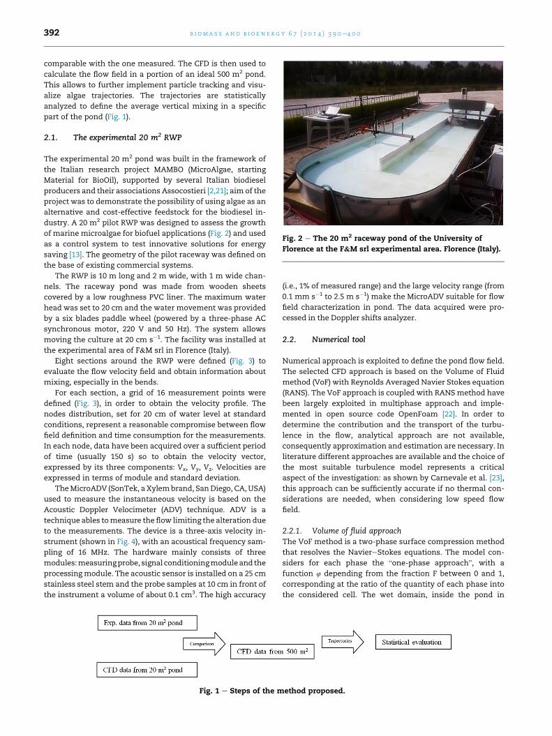
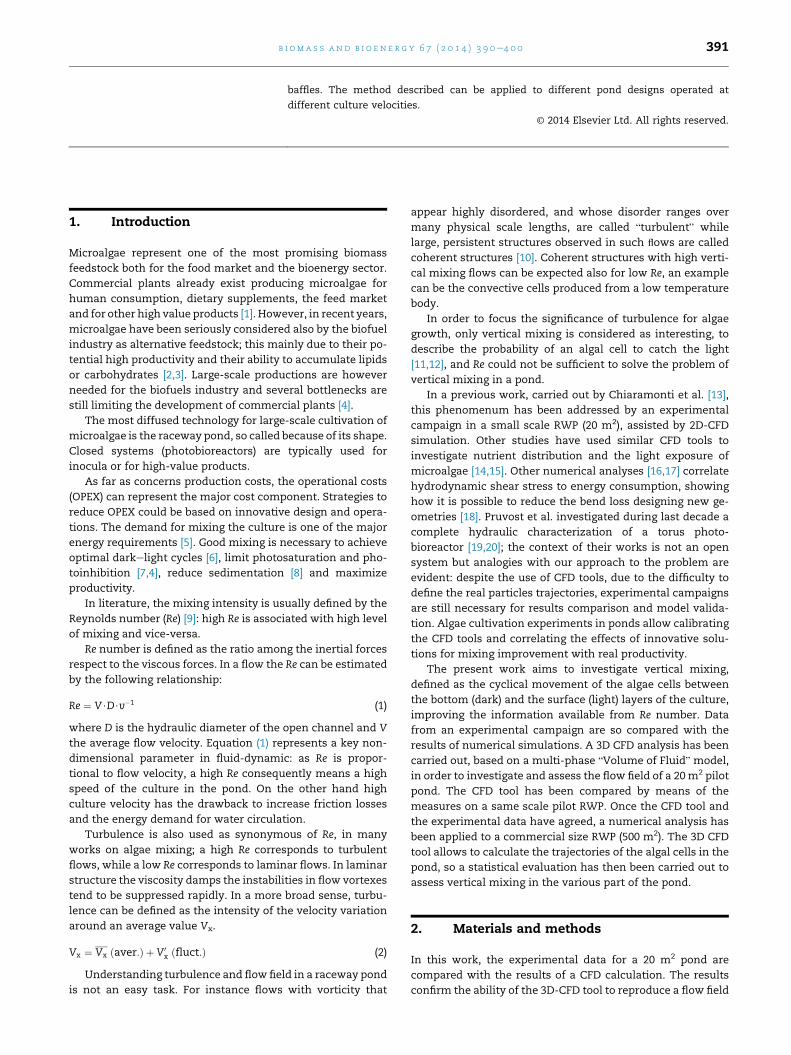
Fig. 2 e The 20 m2 raceway pond of the University of

Florence at the F&M srl experimental area. Florence (Italy).

b i om a s s a n d b i o e n e r g y 6 7 ( 2 0 1 4 ) 3 9 0e4 0 0392

comparable with the one measured. The CFD is then used to

calculate the flow field in a portion of an ideal 500 m2 pond.

This allows to further implement particle tracking and visu-

alize algae trajectories. The trajectories are statistically

analyzed to define the average vertical mixing in a specific

part of the pond (Fig. 1).

2.1. The experimental 20 m2 RWP

The experimental 20 m2 pond was built in the framework of

the Italian research project MAMBO (MicroAlgae, starting

Material for BioOil), supported by several Italian biodiesel

producers and their associations Assocostieri [2,21]; aim of the

project was to demonstrate the possibility of using algae as an

alternative and cost-effective feedstock for the biodiesel in-

dustry. A 20 m2 pilot RWP was designed to assess the growth

of marine microalgae for biofuel applications (Fig. 2) and used

as a control system to test innovative solutions for energy

saving [13]. The geometry of the pilot raceway was defined on

the base of existing commercial systems.

The RWP is 10 m long and 2 m wide, with 1 m wide chan-

nels. The raceway pond was made from wooden sheets

covered by a low roughness PVC liner. The maximum water

head was set to 20 cm and the water movement was provided

by a six blades paddle wheel (powered by a three-phase AC

synchronous motor, 220 V and 50 Hz). The system allows

moving the culture at 20 cm s�1. The facility was installed at

the experimental area of F&M srl in Florence (Italy).

Eight sections around the RWP were defined (Fig. 3) to

evaluate the flow velocity field and obtain information about

mixing, especially in the bends.

For each section, a grid of 16 measurement points were

defined (Fig. 3), in order to obtain the velocity profile. The

nodes distribution, set for 20 cm of water level at standard

conditions, represent a reasonable compromise between flow

field definition and time consumption for the measurements.

In each node, data have been acquired over a sufficient period

of time (usually 150 s) so to obtain the velocity vector,

expressed by its three components: Vx, Vy, Vz. Velocities are

expressed in terms of module and standard deviation.

TheMicroADV (SonTek, a Xylembrand, SanDiego, CA,USA)

used to measure the instantaneous velocity is based on the

Acoustic Doppler Velocimeter (ADV) technique. ADV is a

technique ables tomeasure the flow limiting the alteration due

to the measurements. The device is a three-axis velocity in-

strument (shown in Fig. 4), with an acoustical frequency sam-

pling of 16 MHz. The hardware mainly consists of three

modules:measuringprobe, signal conditioningmoduleand the

processingmodule. The acoustic sensor is installed on a 25 cm

stainless steel stem and the probe samples at 10 cm in front of

the instrument a volume of about 0.1 cm3. The high accuracy

Fig. 1 e Steps of the m

(i.e., 1% of measured range) and the large velocity range (from

0.1 mm s�1 to 2.5 m s�1) make the MicroADV suitable for flow

field characterization in pond. The data acquired were pro-

cessed in the Doppler shifts analyzer.

2.2. Numerical tool

Numerical approach is exploited to define the pond flow field.

The selected CFD approach is based on the Volume of Fluid

method (VoF) with Reynolds Averaged Navier Stokes equation

(RANS). The VoF approach is coupled with RANSmethod have

been largely exploited in multiphase approach and imple-

mented in open source code OpenFoam [22]. In order to

determine the contribution and the transport of the turbu-

lence in the flow, analytical approach are not available,

consequently approximation and estimation are necessary. In

literature different approaches are available and the choice of

the most suitable turbulence model represents a critical

aspect of the investigation: as shown by Carnevale et al. [23],

this approach can be sufficiently accurate if no thermal con-

siderations are needed, when considering low speed flow

field.

2.2.1. Volume of fluid approachThe VoF method is a two-phase surface compression method

that resolves the NaviereStokes equations. The model con-

siders for each phase the “one-phase approach”, with a

function 4 depending from the fraction F between 0 and 1,

corresponding at the ratio of the quantity of each phase into

the considered cell. The wet domain, inside the pond in

ethod proposed.

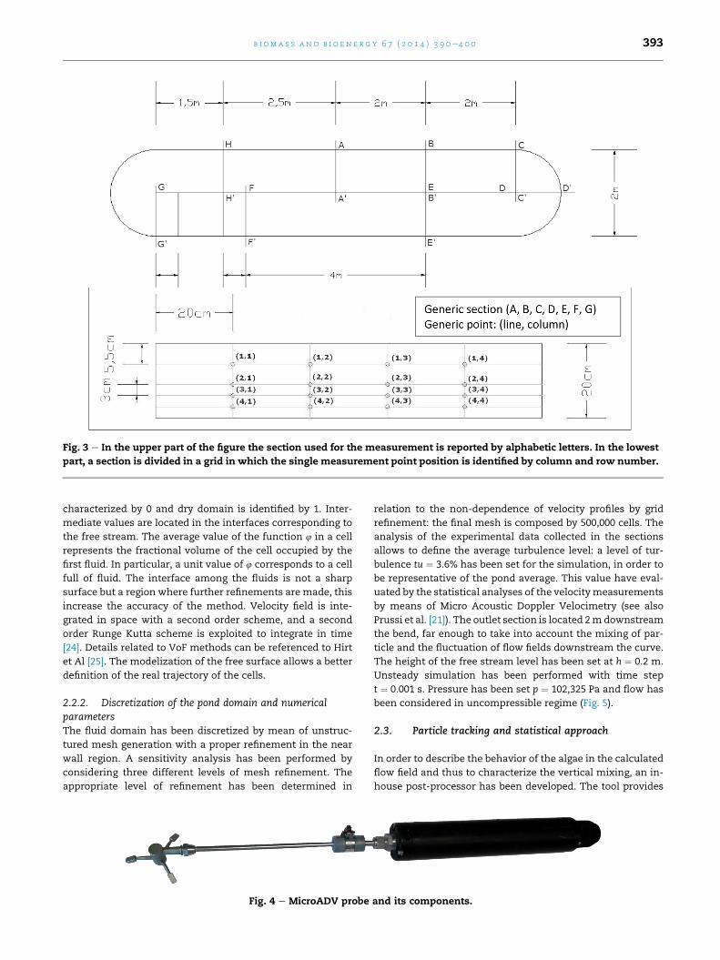
Fig. 3 e In the upper part of the figure the section used for the measurement is reported by alphabetic letters. In the lowest

part, a section is divided in a grid in which the single measurement point position is identified by column and row number.

b i om a s s a n d b i o e n e r g y 6 7 ( 2 0 1 4 ) 3 9 0e4 0 0 393

characterized by 0 and dry domain is identified by 1. Inter-

mediate values are located in the interfaces corresponding to

the free stream. The average value of the function 4 in a cell

represents the fractional volume of the cell occupied by the

first fluid. In particular, a unit value of 4 corresponds to a cell

full of fluid. The interface among the fluids is not a sharp

surface but a region where further refinements are made, this

increase the accuracy of the method. Velocity field is inte-

grated in space with a second order scheme, and a second

order Runge Kutta scheme is exploited to integrate in time

[24]. Details related to VoF methods can be referenced to Hirt

et Al [25]. The modelization of the free surface allows a better

definition of the real trajectory of the cells.

2.2.2. Discretization of the pond domain and numericalparametersThe fluid domain has been discretized by mean of unstruc-

tured mesh generation with a proper refinement in the near

wall region. A sensitivity analysis has been performed by

considering three different levels of mesh refinement. The

appropriate level of refinement has been determined in

Fig. 4 e MicroADV probe

relation to the non-dependence of velocity profiles by grid

refinement: the final mesh is composed by 500,000 cells. The

analysis of the experimental data collected in the sections

allows to define the average turbulence level: a level of tur-

bulence tu ¼ 3.6% has been set for the simulation, in order to

be representative of the pond average. This value have eval-

uated by the statistical analyses of the velocitymeasurements

by means of Micro Acoustic Doppler Velocimetry (see also

Prussi et al. [21]). The outlet section is located 2mdownstream

the bend, far enough to take into account the mixing of par-

ticle and the fluctuation of flow fields downstream the curve.

The height of the free stream level has been set at h ¼ 0.2 m.

Unsteady simulation has been performed with time step

t ¼ 0.001 s. Pressure has been set p ¼ 102,325 Pa and flow has

been considered in uncompressible regime (Fig. 5).

2.3. Particle tracking and statistical approach

In order to describe the behavior of the algae in the calculated

flow field and thus to characterize the vertical mixing, an in-

house post-processor has been developed. The tool provides

and its components.

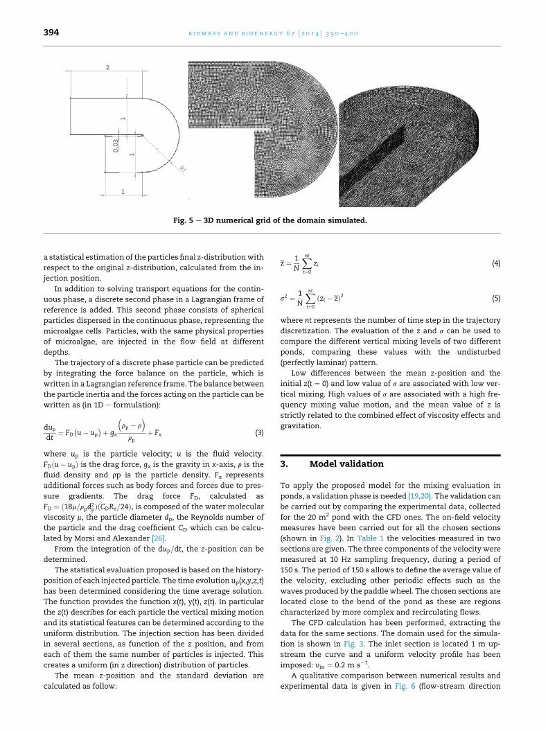
Fig. 5 e 3D numerical grid of the domain simulated.

b i om a s s a n d b i o e n e r g y 6 7 ( 2 0 1 4 ) 3 9 0e4 0 0394

a statistical estimation of the particles final z-distributionwith

respect to the original z-distribution, calculated from the in-

jection position.

In addition to solving transport equations for the contin-

uous phase, a discrete second phase in a Lagrangian frame of

reference is added. This second phase consists of spherical

particles dispersed in the continuous phase, representing the

microalgae cells. Particles, with the same physical properties

of microalgae, are injected in the flow field at different

depths.

The trajectory of a discrete phase particle can be predicted

by integrating the force balance on the particle, which is

written in a Lagrangian reference frame. The balance between

the particle inertia and the forces acting on the particle can be

written as (in 1D e formulation):

dup

dt¼ FD

�u� up

�þ gx

�rp � r

�

rpþ Fx (3)

where up is the particle velocity; u is the fluid velocity.

FDðu� upÞ is the drag force, gx is the gravity in x-axis, r is the

fluid density and rp is the particle density. Fx represents

additional forces such as body forces and forces due to pres-

sure gradients. The drag force FD, calculated as

FD ¼ ð18m=rpd2pÞðCDRe=24Þ, is composed of the water molecular

viscosity m, the particle diameter dp, the Reynolds number of

the particle and the drag coefficient CD which can be calcu-

lated by Morsi and Alexander [26].

From the integration of the dup=dt, the z-position can be

determined.

The statistical evaluation proposed is based on the history-

position of each injected particle. The time evolution up(x,y,z,t)

has been determined considering the time average solution.

The function provides the function x(t), y(t), z(t). In particular

the z(t) describes for each particle the vertical mixing motion

and its statistical features can be determined according to the

uniform distribution. The injection section has been divided

in several sections, as function of the z position, and from

each of them the same number of particles is injected. This

creates a uniform (in z direction) distribution of particles.

The mean z-position and the standard deviation are

calculated as follow:

z ¼ 1 Xntzi (4)

Nt¼0

s2 ¼ 1N

Xntt¼0

ðzi � zÞ2 (5)

where nt represents the number of time step in the trajectory

discretization. The evaluation of the z and s can be used to

compare the different vertical mixing levels of two different

ponds, comparing these values with the undisturbed

(perfectly laminar) pattern.

Low differences between the mean z-position and the

initial z(t ¼ 0) and low value of s are associated with low ver-

tical mixing. High values of s are associated with a high fre-

quency mixing value motion, and the mean value of z is

strictly related to the combined effect of viscosity effects and

gravitation.

3. Model validation

To apply the proposed model for the mixing evaluation in

ponds, a validation phase is needed [19,20]. The validation can

be carried out by comparing the experimental data, collected

for the 20 m2 pond with the CFD ones. The on-field velocity

measures have been carried out for all the chosen sections

(shown in Fig. 2). In Table 1 the velocities measured in two

sections are given. The three components of the velocity were

measured at 10 Hz sampling frequency, during a period of

150 s. The period of 150 s allows to define the average value of

the velocity, excluding other periodic effects such as the

waves produced by the paddle wheel. The chosen sections are

located close to the bend of the pond as these are regions

characterized by more complex and recirculating flows.

The CFD calculation has been performed, extracting the

data for the same sections. The domain used for the simula-

tion is shown in Fig. 3. The inlet section is located 1 m up-

stream the curve and a uniform velocity profile has been

imposed: vin ¼ 0.2 m s�1.

A qualitative comparison between numerical results and

experimental data is given in Fig. 6 (flow-stream direction

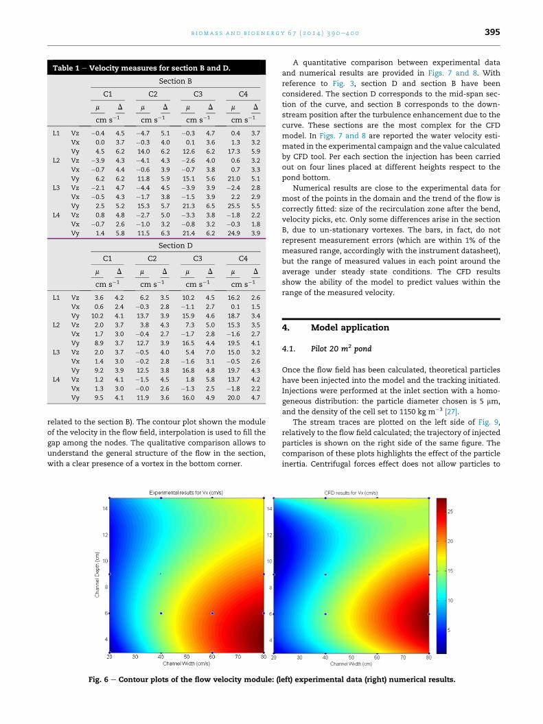
Table 1 e Velocity measures for section B and D.

Section B

C1 C2 C3 C4

m D m D m D m D

cm s�1 cm s�1 cm s�1 cm s�1

L1 Vz �0.4 4.5 �4.7 5.1 �0.3 4.7 0.4 3.7

Vx 0.0 3.7 �0.3 4.0 0.1 3.6 1.3 3.2

Vy 4.5 6.2 14.0 6.2 12.6 6.2 17.3 5.9

L2 Vz �3.9 4.3 �4.1 4.3 �2.6 4.0 0.6 3.2

Vx �0.7 4.4 �0.6 3.9 �0.7 3.8 0.7 3.3

Vy 6.2 6.2 11.8 5.9 15.1 5.6 21.0 5.1

L3 Vz �2.1 4.7 �4.4 4.5 �3.9 3.9 �2.4 2.8

Vx �0.5 4.3 �1.7 3.8 �1.5 3.9 2.2 2.9

Vy 2.5 5.2 15.3 5.7 21.3 6.5 25.5 5.5

L4 Vz 0.8 4.8 �2.7 5.0 �3.3 3.8 �1.8 2.2

Vx �0.7 2.6 �1.0 3.2 �0.8 3.2 �0.3 1.8

Vy 1.4 5.8 11.5 6.3 21.4 6.2 24.9 3.9

Section D

C1 C2 C3 C4

m D m D m D m D

cm s�1 cm s�1 cm s�1 cm s�1

L1 Vz 3.6 4.2 6.2 3.5 10.2 4.5 16.2 2.6

Vx 0.6 2.4 �0.3 2.8 �1.1 2.7 0.1 1.5

Vy 10.2 4.1 13.7 3.9 15.9 4.6 18.7 3.4

L2 Vz 2.0 3.7 3.8 4.3 7.3 5.0 15.3 3.5

Vx 1.7 3.0 �0.4 2.7 �1.7 2.8 �1.6 2.7

Vy 8.9 3.7 12.7 3.9 16.5 4.4 19.5 4.1

L3 Vz 2.0 3.7 �0.5 4.0 5.4 7.0 15.0 3.2

Vx 1.4 3.0 �0.2 2.8 �1.6 3.1 �0.5 2.6

Vy 9.2 3.9 12.5 3.8 16.8 4.8 19.7 4.3

L4 Vz 1.2 4.1 �1.5 4.5 1.8 5.8 13.7 4.2

Vx 1.3 3.0 �0.0 2.6 �1.3 2.5 �1.8 2.2

Vy 9.5 4.1 11.9 3.6 16.0 4.9 20.0 4.7

b i om a s s a n d b i o e n e r g y 6 7 ( 2 0 1 4 ) 3 9 0e4 0 0 395

related to the section B). The contour plot shown the module

of the velocity in the flow field, interpolation is used to fill the

gap among the nodes. The qualitative comparison allows to

understand the general structure of the flow in the section,

with a clear presence of a vortex in the bottom corner.

Fig. 6 e Contour plots of the flow velocity module: (l

A quantitative comparison between experimental data

and numerical results are provided in Figs. 7 and 8. With

reference to Fig. 3, section D and section B have been

considered. The section D corresponds to the mid-span sec-

tion of the curve, and section B corresponds to the down-

stream position after the turbulence enhancement due to the

curve. These sections are the most complex for the CFD

model. In Figs. 7 and 8 are reported the water velocity esti-

mated in the experimental campaign and the value calculated

by CFD tool. Per each section the injection has been carried

out on four lines placed at different heights respect to the

pond bottom.

Numerical results are close to the experimental data for

most of the points in the domain and the trend of the flow is

correctly fitted: size of the recirculation zone after the bend,

velocity picks, etc. Only some differences arise in the section

B, due to un-stationary vortexes. The bars, in fact, do not

represent measurement errors (which are within 1% of the

measured range, accordingly with the instrument datasheet),

but the range of measured values in each point around the

average under steady state conditions. The CFD results

show the ability of the model to predict values within the

range of the measured velocity.

4. Model application

4.1. Pilot 20 m2 pond

Once the flow field has been calculated, theoretical particles

have been injected into the model and the tracking initiated.

Injections were performed at the inlet section with a homo-

geneous distribution: the particle diameter chosen is 5 mm,

and the density of the cell set to 1150 kg m�3 [27].

The stream traces are plotted on the left side of Fig. 9,

relatively to the flow field calculated; the trajectory of injected

particles is shown on the right side of the same figure. The

comparison of these plots highlights the effect of the particle

inertia. Centrifugal forces effect does not allow particles to

eft) experimental data (right) numerical results.

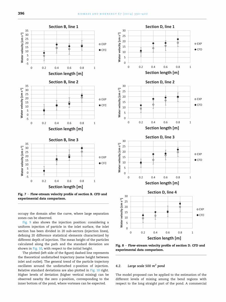
Fig. 7 e Flow-stream velocity profile of section B. CFD and

experimental data comparison.

Fig. 8 e Flow-stream velocity profile of section D. CFD and

experimental data comparison.

b i om a s s a n d b i o e n e r g y 6 7 ( 2 0 1 4 ) 3 9 0e4 0 0396

occupy the domain after the curve, where large separation

zones can be observed.

Fig. 9 also shows the injection position: considering a

uniform injection of particle in the inlet surface, the inlet

section has been divided in 20 sub-sectors (injection lines),

defining 20 difference statistical elements characterized by

different depth of injection. The mean height of the particles

calculated along the path and the standard deviation are

shown in Fig. 10, with respect to the initial height.

The plotted (left side of the figure) dashed line represents

the theoretical undisturbed trajectory (same height between

inlet and outlet). The general trend of the particle trajectory

oscillates around the undisturbed z-position of injection.

Relative standard deviations are also plotted in Fig. 10 right.

Higher levels of deviation (higher vertical mixing) can be

observed nearby the zero z-position, corresponding to the

inner bottom of the pond, where vortexes can be expected.

4.2. Large scale 500 m2 pond

The model proposed can be applied to the estimation of the

different levels of mixing among the bend regions with

respect to the long straight part of the pond. A commercial

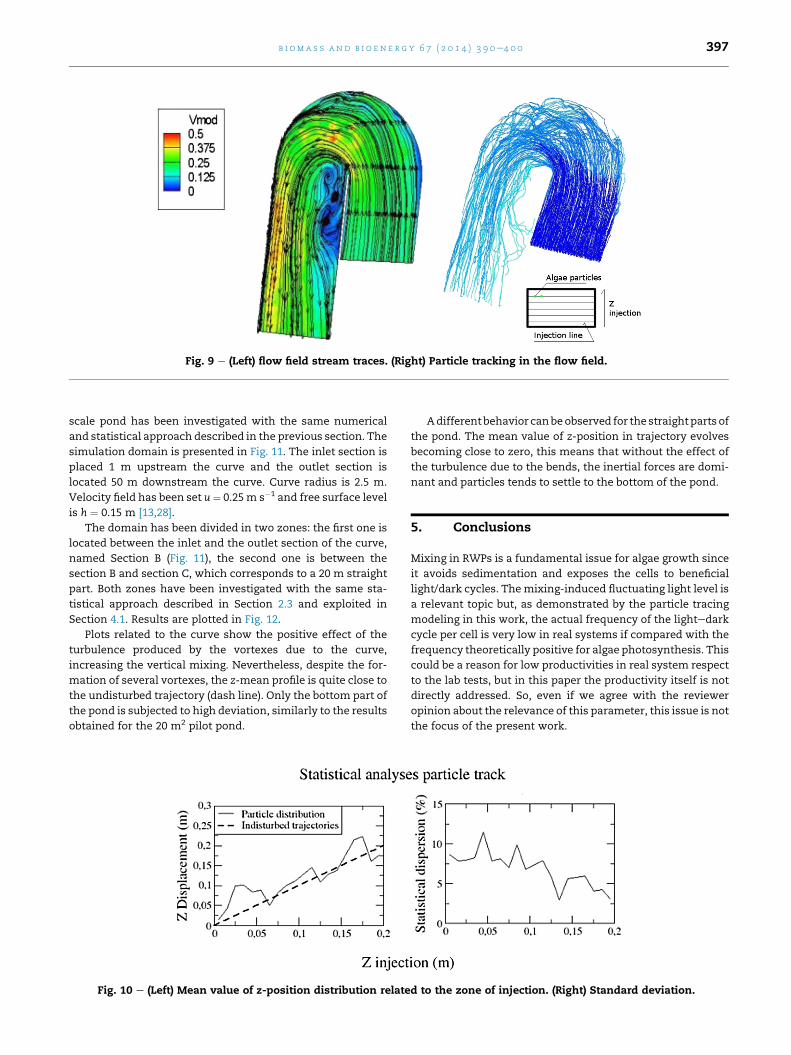
Fig. 9 e (Left) flow field stream traces. (Right) Particle tracking in the flow field.

b i om a s s a n d b i o e n e r g y 6 7 ( 2 0 1 4 ) 3 9 0e4 0 0 397

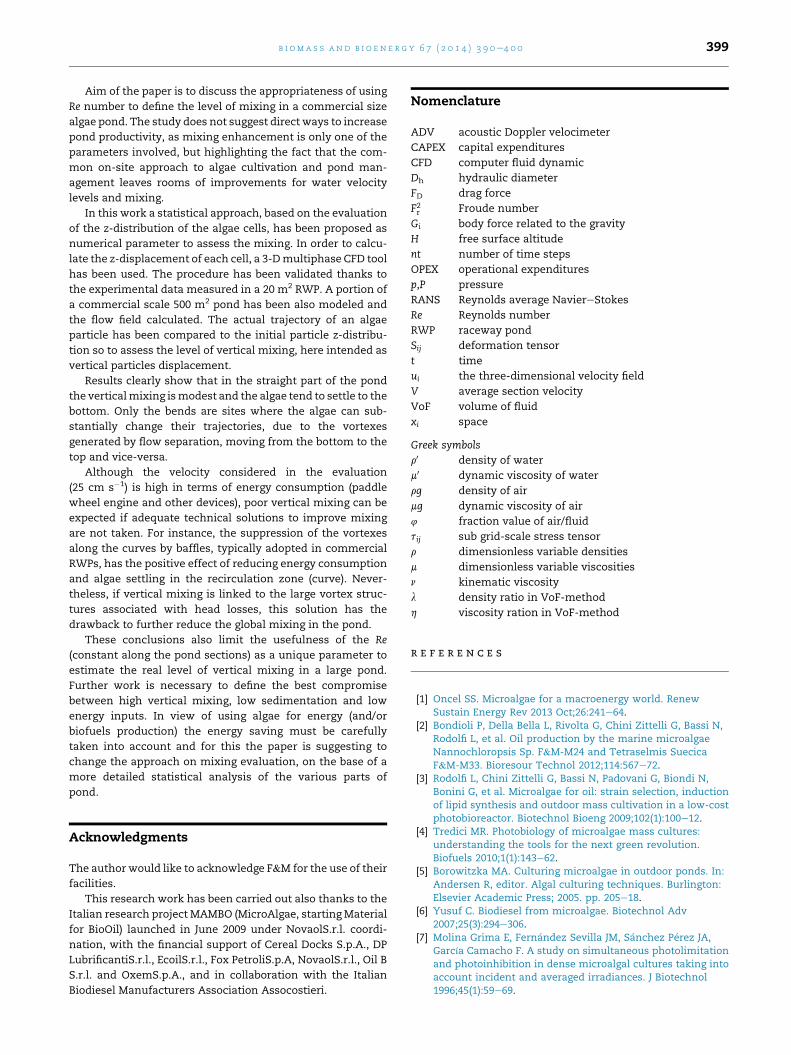
scale pond has been investigated with the same numerical

and statistical approach described in the previous section. The

simulation domain is presented in Fig. 11. The inlet section is

placed 1 m upstream the curve and the outlet section is

located 50 m downstream the curve. Curve radius is 2.5 m.

Velocity field has been set u ¼ 0.25m s�1 and free surface level

is h ¼ 0.15 m [13,28].

The domain has been divided in two zones: the first one is

located between the inlet and the outlet section of the curve,

named Section B (Fig. 11), the second one is between the

section B and section C, which corresponds to a 20 m straight

part. Both zones have been investigated with the same sta-

tistical approach described in Section 2.3 and exploited in

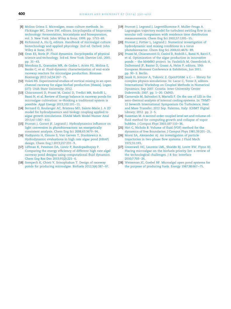
Section 4.1. Results are plotted in Fig. 12.

Plots related to the curve show the positive effect of the

turbulence produced by the vortexes due to the curve,

increasing the vertical mixing. Nevertheless, despite the for-

mation of several vortexes, the z-mean profile is quite close to

the undisturbed trajectory (dash line). Only the bottom part of

the pond is subjected to high deviation, similarly to the results

obtained for the 20 m2 pilot pond.

Fig. 10 e (Left) Mean value of z-position distribution relate

Adifferentbehavior canbeobserved for the straightparts of

the pond. The mean value of z-position in trajectory evolves

becoming close to zero, this means that without the effect of

the turbulence due to the bends, the inertial forces are domi-

nant and particles tends to settle to the bottom of the pond.

5. Conclusions

Mixing in RWPs is a fundamental issue for algae growth since

it avoids sedimentation and exposes the cells to beneficial

light/dark cycles. Themixing-induced fluctuating light level is

a relevant topic but, as demonstrated by the particle tracing

modeling in this work, the actual frequency of the lightedark

cycle per cell is very low in real systems if compared with the

frequency theoretically positive for algae photosynthesis. This

could be a reason for low productivities in real system respect

to the lab tests, but in this paper the productivity itself is not

directly addressed. So, even if we agree with the reviewer

opinion about the relevance of this parameter, this issue is not

the focus of the present work.

d to the zone of injection. (Right) Standard deviation.

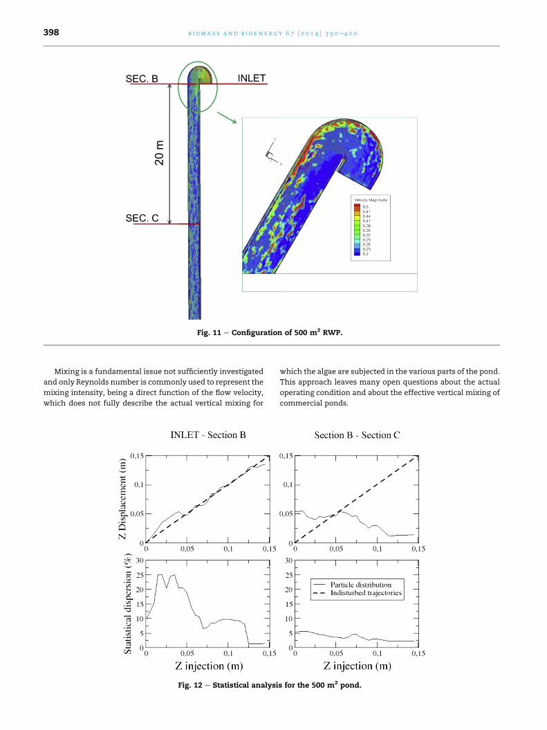
Fig. 11 e Configuration of 500 m2 RWP.

b i om a s s a n d b i o e n e r g y 6 7 ( 2 0 1 4 ) 3 9 0e4 0 0398

Mixing is a fundamental issue not sufficiently investigated

and only Reynolds number is commonly used to represent the

mixing intensity, being a direct function of the flow velocity,

which does not fully describe the actual vertical mixing for

Fig. 12 e Statistical analysi

which the algae are subjected in the various parts of the pond.

This approach leaves many open questions about the actual

operating condition and about the effective vertical mixing of

commercial ponds.

s for the 500 m2 pond.

b i om a s s a n d b i o e n e r g y 6 7 ( 2 0 1 4 ) 3 9 0e4 0 0 399

Aim of the paper is to discuss the appropriateness of using

Re number to define the level of mixing in a commercial size

algae pond. The study does not suggest direct ways to increase

pond productivity, as mixing enhancement is only one of the

parameters involved, but highlighting the fact that the com-

mon on-site approach to algae cultivation and pond man-

agement leaves rooms of improvements for water velocity

levels and mixing.

In this work a statistical approach, based on the evaluation

of the z-distribution of the algae cells, has been proposed as

numerical parameter to assess the mixing. In order to calcu-

late the z-displacement of each cell, a 3-Dmultiphase CFD tool

has been used. The procedure has been validated thanks to

the experimental data measured in a 20 m2 RWP. A portion of

a commercial scale 500 m2 pond has been also modeled and

the flow field calculated. The actual trajectory of an algae

particle has been compared to the initial particle z-distribu-

tion so to assess the level of vertical mixing, here intended as

vertical particles displacement.

Results clearly show that in the straight part of the pond

the verticalmixing ismodest and the algae tend to settle to the

bottom. Only the bends are sites where the algae can sub-

stantially change their trajectories, due to the vortexes

generated by flow separation, moving from the bottom to the

top and vice-versa.

Although the velocity considered in the evaluation

(25 cm s�1) is high in terms of energy consumption (paddle

wheel engine and other devices), poor vertical mixing can be

expected if adequate technical solutions to improve mixing

are not taken. For instance, the suppression of the vortexes

along the curves by baffles, typically adopted in commercial

RWPs, has the positive effect of reducing energy consumption

and algae settling in the recirculation zone (curve). Never-

theless, if vertical mixing is linked to the large vortex struc-

tures associated with head losses, this solution has the

drawback to further reduce the global mixing in the pond.

These conclusions also limit the usefulness of the Re

(constant along the pond sections) as a unique parameter to

estimate the real level of vertical mixing in a large pond.

Further work is necessary to define the best compromise

between high vertical mixing, low sedimentation and low

energy inputs. In view of using algae for energy (and/or

biofuels production) the energy saving must be carefully

taken into account and for this the paper is suggesting to

change the approach on mixing evaluation, on the base of a

more detailed statistical analysis of the various parts of

pond.

Acknowledgments

The author would like to acknowledge F&M for the use of their

facilities.

This research work has been carried out also thanks to the

Italian research project MAMBO (MicroAlgae, startingMaterial

for BioOil) launched in June 2009 under NovaolS.r.l. coordi-

nation, with the financial support of Cereal Docks S.p.A., DP

LubrificantiS.r.l., EcoilS.r.l., Fox PetroliS.p.A, NovaolS.r.l., Oil B

S.r.l. and OxemS.p.A., and in collaboration with the Italian

Biodiesel Manufacturers Association Assocostieri.

Nomenclature

ADV acoustic Doppler velocimeter

CAPEX capital expenditures

CFD computer fluid dynamic

Dh hydraulic diameter

FD drag force

F2r Froude number

Gi body force related to the gravity

H free surface altitude

nt number of time steps

OPEX operational expenditures

p,P pressure

RANS Reynolds average NaviereStokes

Re Reynolds number

RWP raceway pond

Sij deformation tensor

t time

ui the three-dimensional velocity field

V average section velocity

VoF volume of fluid

xi space

Greek symbols

r0 density of water

m0 dynamic viscosity of water

rg density of air

mg dynamic viscosity of air

4 fraction value of air/fluid

tij sub grid-scale stress tensor

r dimensionless variable densities

m dimensionless variable viscosities

n kinematic viscosity

l density ratio in VoF-method

h viscosity ration in VoF-method

r e f e r e n c e s

[1] Oncel SS. Microalgae for a macroenergy world. RenewSustain Energy Rev 2013 Oct;26:241e64.

[2] Bondioli P, Della Bella L, Rivolta G, Chini Zittelli G, Bassi N,Rodolfi L, et al. Oil production by the marine microalgaeNannochloropsis Sp. F&M-M24 and Tetraselmis SuecicaF&M-M33. Bioresour Technol 2012;114:567e72.

[3] Rodolfi L, Chini Zittelli G, Bassi N, Padovani G, Biondi N,Bonini G, et al. Microalgae for oil: strain selection, inductionof lipid synthesis and outdoor mass cultivation in a low-costphotobioreactor. Biotechnol Bioeng 2009;102(1):100e12.

[4] Tredici MR. Photobiology of microalgae mass cultures:understanding the tools for the next green revolution.Biofuels 2010;1(1):143e62.

[5] Borowitzka MA. Culturing microalgae in outdoor ponds. In:Andersen R, editor. Algal culturing techniques. Burlington:Elsevier Academic Press; 2005. pp. 205e18.

[6] Yusuf C. Biodiesel from microalgae. Biotechnol Adv2007;25(3):294e306.

[7] Molina Grima E, Fern�andez Sevilla JM, S�anchez P�erez JA,García Camacho F. A study on simultaneous photolimitationand photoinhibition in dense microalgal cultures taking intoaccount incident and averaged irradiances. J Biotechnol1996;45(1):59e69.

b i om a s s a n d b i o e n e r g y 6 7 ( 2 0 1 4 ) 3 9 0e4 0 0400

[8] Molina Grima E. Microalgae, mass culture methods. In:Flickinger MC, Drew SW, editors. Encyclopedia of bioprocesstechnology: fermentation, biocatalysis and bioseparation,vol. 3. New York: John Wiley & Sons; 1999. pp. 1753e69.

[9] Richmond A, Hu Q, editors. Handbook of microalgal culture:biotechnology and applied phycology. 2nd ed. Oxford: JohnWiley & Sons; 2013.

[10] Oran ES, Boris JP. Fluid dynamics. Encyclopedia of physicalscience and technology. 3rd ed. New York: Elsevier Ltd.; 2001.pp. 31e43.

[11] Mendoza JL, Granados MR, de Godos I, Aci�en FG, Molina E,Banks C, et al. Fluid-dynamic characterization of real-scaleraceway reactors for microalgae production. BiomassBioenergy 2013 Jul;54:267e75.

[12] Voleti RS. Experimental studies of vertical mixing in an openchannel raceway for algae biofuel production [thesis]. Logan(UT): Utah State University; 2012.

[13] Chiaramonti D, Prussi M, Casini D, Tredici MR, Rodolfi L,Bassi N, et al. Review of Energy balance in raceway ponds formicroalgae cultivation: re-thinking a traditional system ispossible. Appl Energy 2013;102:101e11.

[14] Bernard O, Boulanger AC, Bristeau MO, Sainte-Marie J. A 2Dmodel for hydrodynamics and biology coupling applied toalgae growth simulations. ESAIM Math Model Numer Anal2013;47:1387e412.

[15] Pruvost J, Cornet JF, Legrand J. Hydrodynamics influence onlight conversion in photobioreactors: an energeticallyconsistent analysis. Chem Eng Sci 2008;63:3679e94.

[16] Hadiyanto H, Elmore S, Van Gerven T, Stankiewicz A.Hydrodynamic evaluations in high rate algae pond (HRAP)design. Chem Eng J 2013;217:231e9.

[17] Liffman K, Paterson DA, Liovic P, Bandopadhayay P.Comparing the energy efficiency of different high rate algalraceway pond designs using computational fluid dynamics.Chem Eng Res Des 2013;91(2):221e6.

[18] Sompech K, Chisti Y, Srinophakun T. Design of racewayponds for producing microalgae. Biofuels 2012;3(4):387e97.

[19] Pruvost J, Legrand J, Legentilhomme P, Muller-Feuga A.Lagrangian trajectory model for turbulent swirling flow in anannular cell: comparison with residence time distributionmeasurements. Chem Eng Sci 2002;57:1205e15.

[20] Pruvost J, Pottier L, Legrand J. Numerical investigation ofhydrodynamic and mixing conditions in a torusphotobioreactor. Chem Eng Sci 2006;61:4476e89.

[21] Prussi M, Chiaramonti D, Casini D, Rodolfi L, Bassi N, Bacci F,et al. Optimization of the algae production in innovativeponds e the MAMBO project. In: Faulstich M, Ossenbrink H,Dallemand JF, Baxter D, Grassi A, Helm P, editors. 19thEuropean Biomass Conference & Exhibition; Jun 2011.pp. 90e3. Berlin.

[22] Jasak H, Jemcov A, Tukovic Z. OpenFOAM: a Cþþ library forcomplex physics simulations. In: Lacor C, Terze Z, editors.International Workshop on Coupled Methods in NumericalDynamics; Sep 2007. Croatia: Inter-University CenterDubrovnik; 2007. pp. 1e20. CMND.

[23] Carnevale M, Salvadori S, Martelli F. On the use of LES in theaero-thermal analysis of internal cooling systems. In: THMT-12 Seventh International Symposium On Turbulence, Heatand Mass Transfer; 2012 Sep. Palermo, Italy: ICHMT DigitalLibrary; 2012. pp. 2e5.

[24] Sussman M. A second order coupled level set and volume-of-fluid method for computing growth and collapse of vaporbubbles. J Comput Phys 2003;187:110e36.

[25] Hirt C, Nichols B. Volume of fluid (VOF) method for thedynamics of free Boundaries. J Comput Phys 1981;39:201e25.

[26] Morsi SA, Alexander AJ. An investigation of particletrajectories in two-phase flow systems. J Fluid Mech1972;55:193.

[27] Greenwell HC, Laurens LML, Shields RJ, Lovitt RW, Flynn KJ.Placing microalgae on the biofuels priority list: a review ofthe technological challenges. J R Soc Interface2010;7:703e26.

[28] Weissman JC, Goebel RP. Microalgal open pond systems forthe purpose of producing fuels. Energy 1987;98:667e75.