CONFIDENTIAL UP TO AND INCLUDING 12/31/2014 - DO NOT COPY, DISTRIBUTE OR MAKE PUBLIC IN ANY WAY

Experimental and numerical study of storage racking

systems in earthquake situation

Kenny Martens

Promotor: prof. Hervé Degée

Begeleider: ir. Catherine Braham

Masterproef ingediend tot het behalen van de academische graad van

Master in de ingenieurswetenschappen: bouwkunde

Vakgroep Bouwkundige Constructies

Voorzitter: prof. dr. ir. Luc Taerwe

Faculteit Ingenieurswetenschappen en Architectuur

Academiejaar 2012-2013

CONFIDENTIAL UP TO AND INCLUDING 12 / 31 / 2014

IMPORTANT

This Master Dissertation may contain confidential information and/or confidential research results

proprietary to Ghent University or third parties. It is strictly forbidden to publish, cite or make public

in any way this Master Dissertation or any part thereof without the express written permission of

Ghent University. Under no circumstance this Master Dissertation may be communicated to or put at

the disposal of third parties. Photocopying or duplicating it in any other way is strictly prohibited.

Disregarding the confidential nature of this Master Dissertation may cause irremediable damage to

Ghent University.

CONFIDENTIAL UP TO AND INCLUDING 12/31/2014 - DO NOT COPY, DISTRIBUTE OR MAKE PUBLIC IN ANY WAY

Experimental and numerical study of storage racking

systems in earthquake situation

Kenny Martens

Promotor: prof. Hervé Degée

Begeleider: ir. Catherine Braham

Masterproef ingediend tot het behalen van de academische graad van

Master in de ingenieurswetenschappen: bouwkunde

Vakgroep Bouwkundige Constructies

Voorzitter: prof. dr. ir. Luc Taerwe

Faculteit Ingenieurswetenschappen en Architectuur

Academiejaar 2012-2013

i

Preface

In this paragraph, I will take the opportunity to state a word of thanks to the people who played an

important role in my life and especially during the development of this master dissertation.

First of all, I want to thank my supervisor and mentor Prof. Hervé Degée from the University of Liège

for leading and supporting me during the development of this master dissertation. His experience on

the field and good surveillance of my work really made a significant tribute. In this light, I would also

like to thank Ir. Catherine Braham from the University of Liège who supported me on establishing

numerical models.

Second, a word of thanks goes to all people that are related to the SEISRACKS 2-project I met at the

meeting in Aachen. This meeting was a good experience and gave me an idea in what context my

master dissertation resides.

I would like to state special thanks to my parents Johny and Rosa who gave me the opportunity to

study at Ghent University and who firmly supported me during my study at the university. I also want

to thank my sister Joyce for being there when I needed her and helping me to get on track in my first

year at Ghent University. As a matter of fact, she was the ideal example to follow during my whole

education.

Finally, I want to thank my girlfriend Elien for being there for me in hard times. Especially in the last

months before the deadline she was a really good support, friend and outlet to me.

ii

Admission to loan

"The author gives permission to make this master dissertation available for consultation and to copy

parts of this master dissertation for personal use. In the case of any other use, the limitations of the

copyright have to be respected, in particular with regard to the obligation to state expressly the

source when quoting results from this master dissertation."

"De auteur geeft de toelating deze masterproef voor consultatie beschikbaar te stellen en delen van

de masterproef te kopiëren voor persoonlijk gebruik. Elk ander gebruik valt onder de beperkingen van

het auteursrecht, in het bijzonder met betrekking tot de verplichting de bron uitdrukkelijk te

vermelden bij het aanhalen van resultaten uit deze masterproef."

Ghent, June 2013

Kenny Martens

iii

Experimental and numerical study of storage racking systems

in earthquake situation

Kenny Martens

Promotor: prof. Hervé Degée

Begeleider: ir. Catherine Braham

Masterproef ingediend tot het behalen van de academische graad van

Master in de ingenieurswetenschappen: bouwkunde

Vakgroep Bouwkundige Constructies

Voorzitter: prof. dr. ir. Luc Taerwe

Faculteit Ingernieurswetenschappen en Architectuur

Academiejaar 2012-2013

Summary

This master dissertation deals with the numerical analysis of storage racking systems in seismic areas

and takes part in the research project 'Storage racks in seismic areas 2', launched in 2011 by the

European Union. For the four participating producers in the research project, a 2D model was

created in the software package FineLg. With this software package, a determined series of

numerical analyses was performed for each product. These analyses are a modal analysis, monotonic

linear and nonlinear analyses. Furthermore, two payload cases are considered: a fully loaded case

and a top loaded case. Also, for illustrative reasons, cyclic and dynamic analyses were performed for

one product for the fully loaded case. The main result of the analyses is translated into load-

displacement curves. From these results, evaluation of the behaviour of the typical storage racking

systems of each producer and comparison between them was performed from different points of

view. Products A, C and D are low seismicity systems and product B is a high seismicity system.

The analyses lead to the first conclusion that the fully loaded case is the most critical payload case for

the design of storage racking systems in earthquake situation. The overall behaviour of all four

products is approximate the same. All storage racks suffered significant second order effects,

products C and D suffering the most. The performance of products C and D is similar to each other,

while the performance of product A shows similarities with products C and D, but also with product

B. The performance of product A is found to be slightly better than that of products C and D. Being a

high seismicity system, product B allows larger displacements and absorbs more energy upon failure.

Finally, the design of product B turns out to be the least (but still) conservative for its applied seismic

action whereas the other three products are more conservatively designed. The cyclic analyses

resulted in a good fit between the load-displacement curves and the monotonic pushover curves. It

was concluded that the design of product B was conservative. The dynamic analysis illustrated

significant damping due to the yielding of column base and/or beam-to-column connections.

Keywords

Numerical, storage racks, seismic areas, comparison, second order effects, performance.

iv

Experimental and numerical study of

storage racking systems in earthquake

situation

Kenny Martens

Supervisors: Prof. Hervé Degée, Ir. Catherine Braham

Abstract: Specific design rules have to be added

to Eurocode 8[1]

for the design of storage racking

systems in earthquake situation. In order to make

this possible, the SEISRACKS 2-project was

established wherein this dissertation takes part.

For four products involved in the project,

numerical analyses were performed on 2D

models in the down-aisle direction, for two

payload cases. These analyses lead to the

conclusion that the fully loaded payload case is

the most critical design case. Furthermore,

significant second order effects were encountered

for all products. All products were found to be

conservatively designed for the applied seismic

action. Finally, it is concluded that the

performance of product A was slightly better than

products C and D, while C and D have similar

performance. Product B was most optimally

designed for the applied seismic action.

Keywords: Numerical, storage racks, seismic,

comparison, second order effects, performance.

I. Introduction

Nowadays, steel storage racking systems are

extensively used in a large variety of facilities

and stores. Since about the year 2000, these

storage racks have grown in height and are

placed more and more in public spaces. As a

result of this tendency, the risk for human injuries

and loss of valuable goods when these storage

systems fail has grown significantly. The most

critical environment for a storage rack to fail is

obviously the usage of such a system in seismic

active zones, as the rack can fail under seismic

loading and the stored goods can fall off. In

Eurocode 8[1]

, design rules are stated for the

design of typical buildings in seismic areas. But

these design rules cannot be applied for storage

racking systems, as these systems show

significant differences with typical buildings.

Therefore, the European Union decided that

specific design rules for storage racking systems

in seismic areas had to be established. To achieve

these design rules, the EU set up a first research

project in 2004 titled 'Storage Racks in Seismic

Areas' or abbreviated SEISRACKS[2]

. The

project ended in 2007 and resulted in a draft of

the FEM 10.2.08 'Recommendations for the

design of static steel pallet racks under seismic

conditions'[3]

. In September 2010, the first

version of FEM 10.2.08[4]

was published. The

next goal of the EU is to convert this code of

practice into a section of Eurocode 8[1]

. In order

to fill up the remaining gaps and to optimize the

existing recommendations, a second research

project was set up in 2011, titled SEISRACKS 2.

One of the work packages of this project is

devoted to numerical analysis. In this

dissertation, being part of that work package, 2D

models are build in the software tool FineLg[5]

for

four different products. Because of

confidentiality reasons, the products are named

product A, B, C and D. With these models,

monotonic analyses were performed resulting in

load-displacement curves from which general

conclusions about the behaviour of the different

storage racking systems were drawn.

II. 2D models and types of analysis

v

A. 2D models

For each product, one 2D model with two bays

and four levels was created in FineLg[5]

. The

uprights and pallet beams are modelled as

rectangular sections, having the same area and

second moment of area as the real upright and

pallet beam sections. The beam-to-column

connections and the column base connections to

the floor level are typically modelled as rotation

springs. An example of such a model is shown in

the figure below (Figure 1).

Figure 1: 2D model

The moment-rotation characteristics for the

beam-to-column rotation springs are adopted

from test results of experimental component tests

performed within the SEISRACKS 2 project[6]

.

For the column base connections, the information

is adopted from designer's sheets as the

corresponding component tests were not finished

yet at the time of performing these analyses. The

payload on the storage racks exists out of three

pallets per bay and level, with a maximum mass

of 800 kg each pallet. In the numerical model,

this 'unit payload' is modelled as a concentrated

mass of 400 kg for the modal analysis and as

three vertical forces of 1.308 kN for the other

analyses. The seismic action in the analyses is

modelled as a set of triangularly distributed

forces determined according to Eurocode 8[1]

.

These horizontal forces apply at each beam level

as is shown in the figure below (Figure 2).

Figure 2: Seismic action

For the calculation of the seismic action, it is

mentioned that products A, C and D are low

seismicity systems and product B a high

seismicity system. As a result, a response

spectrum type 2 is chosen for the low seismicity

systems and a type 1 is chosen for product B. All

storage racks are assumed to be placed on soil

type C.

B. Types of analysis

For each 2D model, two payload cases are

considered, being a fully loaded and a top loaded

case. In all analyses, the uprights and pallet

beams are assumed to behave linear elastic. The

assumption of the connection behaviour is

different for different types of analysis. For each

model and payload case, a series of analyses is

performed in a fixed order. First, a modal

analysis is performed resulting in the knowledge

of the first mode. With this first mode, the

seismic action can be calculated according to

Eurocode 8[1]

.

Second, a series of monotonic analyses were

performed: a linear elastic and a nonlinear elastic

analysis, assuming that the connections behave

elastic; a nonlinear analysis wherein the

connectors are modelled to have an elastic-

perfectly plastic material law (material law 1 in

FineLg) and a nonlinear analysis wherein the

beam-to-column connections are modelled to

have a piecewise linear material law (material

law 11 in FineLg) and the column base

connections an elastic-perfectly plastic material

law. Finally, illustrative cyclic and dynamic

vi

analyses were performed for product B for the

fully loaded case. As the research in this

dissertation was concentrated on monotonic

analyses, the cyclic and dynamic analyses are not

included in this paper.

III. Results and discussion

A. Modal analysis and seismic action

The modal analysis resulted in high values for the

first period for all products and payload cases.

The first periods were all situated between 2 and

3 seconds for the fully loaded case and between

1.7 and 2.2 seconds for the top loaded case. The

highest periods were observed for products C and

D. The percentages of collaborate mass for the

first modes all lie around 85% for the fully

loaded case. There is only one mode in the top

loaded case, so this percentage is 100%. It was

assumed that the percentage of collaborate mass

for the fully loaded case was close enough to

90% in order to calculate the seismic action

according to the first period. The following

seismic actions were imposed on the models

(Tables 1 and 2).

Table 1 : Seismic action (fully loaded case) [kN]

Product F1 F2 F3 F4

A 0.152 0.304 0.456 0.608

B 0.509 1.032 1.555 2.078

C 0.222 0.451 0.679 0.908

D 0.181 0.367 0.554 0.741

Table 2 : Seismic action (top loaded case) [kN]

Product F4

A 0.380

B 1.907

C 0.565

D 0.461

The seismic action for product B is obviously

bigger as a type 1 response spectrum is used.

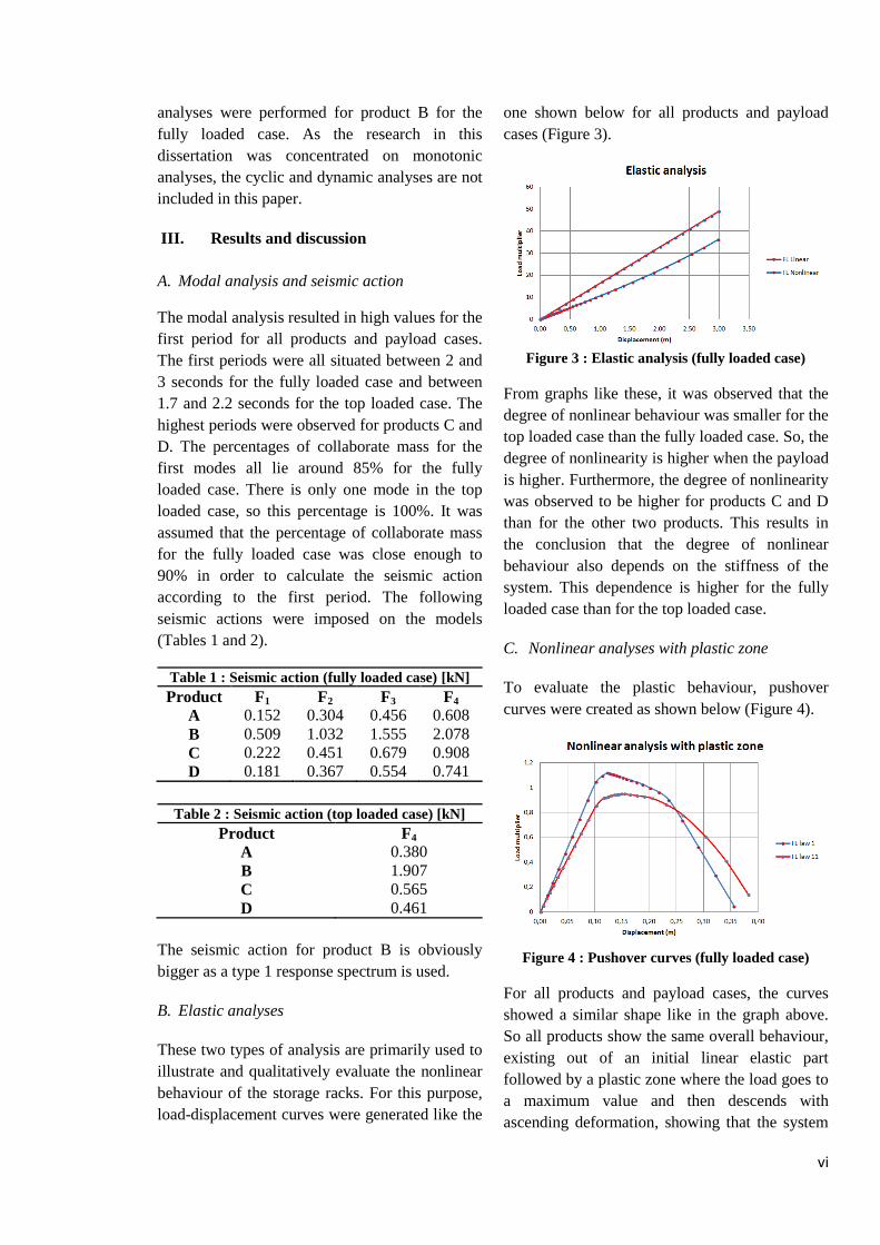
B. Elastic analyses

These two types of analysis are primarily used to

illustrate and qualitatively evaluate the nonlinear

behaviour of the storage racks. For this purpose,

load-displacement curves were generated like the

one shown below for all products and payload

cases (Figure 3).

Figure 3 : Elastic analysis (fully loaded case)

From graphs like these, it was observed that the

degree of nonlinear behaviour was smaller for the

top loaded case than the fully loaded case. So, the

degree of nonlinearity is higher when the payload

is higher. Furthermore, the degree of nonlinearity

was observed to be higher for products C and D

than for the other two products. This results in

the conclusion that the degree of nonlinear

behaviour also depends on the stiffness of the

system. This dependence is higher for the fully

loaded case than for the top loaded case.

C. Nonlinear analyses with plastic zone

To evaluate the plastic behaviour, pushover

curves were created as shown below (Figure 4).

Figure 4 : Pushover curves (fully loaded case)

For all products and payload cases, the curves

showed a similar shape like in the graph above.

So all products show the same overall behaviour,

existing out of an initial linear elastic part

followed by a plastic zone where the load goes to

a maximum value and then descends with

ascending deformation, showing that the system

vii

is evolving into a mechanism. In reality the

curves shown above are cut off at the point where

failure of the system occurs (see further section).

From the graphs, it is observed that for all

products the curve maxima for 'law 11' are

shifted to larger displacements than those of 'law

1'. For the top loaded case, these displacement

values are higher than observed in the fully

loaded case. The highest displacements were

observed for product B in both payload cases. For

products A, C and D, these values were

approximate the same in the fully loaded case.

For the top loaded case, the values for products C

and D were almost the same as for product B and

product A showed the lowest displacements.

Considering the load multiplier, it is observed

that the curve maximum for 'law 11' is lower than

for 'law 1' for products A, C and D in the fully

loaded case. But, as both curves meet after

reaching their maximum, it is concluded that for

these cases, the more realistic model (law 11)

exhibits a certain understrength but possesses a

better plastic behaviour than the design model

(law 1). For product B in the fully loaded case

and all products in the top loaded case, the 'law

11' curve reaches a higher maximum en exhibits

similar plastic behaviour as the 'law 1' curve.

Comparing the seismic actions between both

payload cases shows that the maximum seismic

action is larger for the top loaded case. The

difference with the fully loaded case is smallest

for products A and B, indicating that the

influence of the payload is smaller for systems

with higher stiffness.

Considering the amount of energy absorbed

during the tests, one can see that the area under

both curves is approximate the same for products

A, C and D in the fully loaded case. For product

B in the fully loaded case and all products in the

top loaded case, the area under the curves and

thus the absorbed energy is larger for the more

realistic model (law 11). Furthermore, product B

absorbs most energy in both payload cases. It is

also observed that more energy is absorbed in the

top loaded cases than in the fully loaded cases.

D. Calculation of parameters

In order to achieve an accurate evaluation of the

behaviour, three parameters are calculated. These

are the interstorey drift sensitivity factor ,

the plastic failure load factor and the

performance point . For the calculation method

of these parameters, reference is made to FEM

10.2.08[4]

for , Eurocode 8[1]

for and the

course 'Nonlinear and plastic methods of

structural analysis'[7]

for .

In the tables below, the interstorey drift

sensitivity factors are given (Tables 3 and 4).

Table 3: -values (fully loaded case) [-]

Product Storey 1 Storey 2 Storey 3 Storey 4 A 0.498 0.413 0.354 0.309 B 0.523 0.423 0.362 0.316 C 0.620 0.501 0.429 0.375 D 0.806 0.649 0.556 0.485

Table 4: -values (top loaded case) [-]

Product Storey 1 Storey 2 Storey 3 Storey 4 A 0.210 0.209 0.209 0.209 B 0.207 0.202 0.202 0.202 C 0.237 0.230 0.230 0.230 D 0.310 0.300 0.300 0.300

In the tables above, one can observe that the

maximum values are found for the first storey.

Furthermore, the largest values are seen for

product D and the lowest for products A and B.

So, the more stiff the system, the smaller the

second order effects. For the fully loaded case,

the second order effects are highest for the first

storey and are diminishing with increasing level.

For the top loaded case, the second order effects

are evenly distributed among the storeys.

Comparing the -values with the

classification of table 2.9 of FEM 10.2.08[4]

, it is

concluded (as all q-factors are lower or equal to

2.0) that in the fully loaded case the second order

effects are to be explicitly considered in the

analysis by means of geometrically nonlinear

analysis. As the values for products C and D are

very high, it is stated that these storage racks

require horizontal bracing in down-aisle direction

in order to improve the overall stiffness of the

system. For the top loaded payload case, it is

viii

stated that the second order effects can be

approximately taken into account by multiplying

the seismic action by a factor of 1/(1- ) for

product A, B and C. For product D the same can

be stated for the three upper storeys. For the first

storey, it is recommended to perform a

geometrically nonlinear analysis. Finally, it is

observed that the top loaded case suffers less

second order effects than the fully loaded case.

E. Synthesis

Now, all analyses done are summarized in one

graph together with the plastic failure load factor

and the performance point. Also, all curves are

cut off at the point of first component failure. An

example is given in the figure below (Figure 5).

Figure 5: Synthesis (fully loaded case)

For all products and payload cases, it was

observed that the plastic failure load factors are

situated high above the curve maxima. So all

products suffer second order effects, which is in

agreement with the interstorey drift sensitivity

factors. The difference between these failure load

factors and the curve maxima is largest for

products C and D and smallest for product B.

Also, it is observed that second order effects have

a bigger impact in the realistic model (law 11)

than in the design model (law 1). Finally, it is

observed that all top loaded models suffer less

second order effects than their fully loaded

counterparts.

Considering the performance points on the

graphs, it is noticed that for all products and

payload cases, these points are situated at the left

side of the curve maxima. This means that all

products meet the seismic demand in terms of

displacement. For products A, C and D, the

performance point is situated in the elastic zone

of the curves, meaning that the design is very

conservative for the applied seismic action. For

product B, the performance point is situated in

the plastic region for the fully loaded case. For

the top loaded case, the performance point is also

situated in the elastic region. Product B is most

optimally and least conservatively designed

when comparison is made among the products.

Furthermore, it is observed that the seismic

demand is bigger for the fully loaded case than

the top loaded case.

Finally, an evaluation of first component failure

was performed. In the fully loaded payload case,

the first component that failed was the interior

column base connection. In the top loaded

condition, this was also the case for products C

and D. For product A, the first components that

failed were some first level and second level

beam-to-column connectors and for product B

the interior column base connection and some top

level connectors. Comparing the cut off points

with the curve maxima by means of displacement

gives a first idea of the ductility of the systems. It

was observed that product A exhibited the most

and products B and D the least ductile behaviour

in the fully loaded case. In the top loaded case,

products A and B exhibited most ductility.

Furthermore it was observed that the cut-off

points are situated at higher displacements and

shear loads in the top loaded case than in the

fully loaded case. Moreover, the ductility of the

systems seemed to be higher in the top loaded

case.

IV. Conclusions

From the analyses above, it is concluded that the

fully loaded payload case is the most critical

payload case for the design of storage racking

systems in earthquake situation. The overall

behaviour of the storage racking systems is

approximate the same. All products suffer

significant second order effects, products C and

D suffering the most. The design of all products

ix

is conservative for the applied seismic action,

product B being the least conservative. The

overall performance of products C and D is

similar. The performance of product A (being

slightly better than C and D) showed similarities

with products C and D , but also with product B.

Being a high seismicity system, product B

allowed most displacement and absorbed most

energy upon failure.

Acknowledgements

The work was carried out within the framework

of a Master dissertation at the Faculty of

Engineering and Architecture of Ghent

University, in partnership with the ArGEnCo

department of the University of Liège.

References

[1] EN 1998 - Eurocode 8. "Design of structures

for earthquake resistance." European

Committee for Standardisation, Brussels,

2005.

[2] Ing. I. Rosin, Geom. G. Coracina, Prof. L.

Calado, Prof. J. Proença, Prof. P. Carydis,

Prof. H. Mouzakis, Prof. C. Castiglioni, Dr.

J.C. Brescianini, Prof. A. Plumier, Prof. H.

Degée, Dr. P. Negro, Dr. F. Molina. "Storage

Racks in Seismic Areas, Final Report."

Research Fund for Coal and Steel, 2007.

[3] Pr FEM 10.2.08. "Recommendations for the

Design of Static Steel Pallet Racks under

Seismic Conditions." European Federation of

Materials Handling, 2008.

[4] FEM 10.2.08. "Recommendations for the

Design of Static Steel Pallet Racks under

Seismic Conditions." European Federation of

Materials Handling, 2010.

[5] "FineLg, V9.3 ." Software package,

Department ArGEnCo - University of Liège

and Engineering Office Greisch, Liège.

[6] Feldmann M., Heinemeyer C., Hofmeister B.

"Seisracks 2: Tests on Seismic Performance of

Racks, Beam End Connectors in Down Aisle

Direction." Institut und Lehrstuhl für Stahlbau

und Leichtmetallbau, Aachen, 2013.

[7] Prof. Dr. Ir. Rudy Van Impe., Prof. Dr. Ir. Luc

Taerwe. "Nonlinear and Plastic Methods of

Structural Analysis." Course, Faculty of

Engineering and Architecture, Ghent

University, 2012-2013.

x

Experimentele en numerieke studie van

reksystemen in

aardbevingsomstandigheden

Kenny Martens

Promotor: Prof. Hervé Degée; Begeleider: Ir. Catherine Braham

Abstract: Specifieke ontwerpregels moeten

toegevoegd worden aan Eurocode 8[1]

voor het

ontwerp van reksystemen die blootgesteld worden

aan aardbevingen. Daartoe werd het

onderzoeksproject SEISRACKS 2 opgezet

waarvan dit eindwerk deel uitmaakt. Numerieke

analyses werden gedaan voor de producten van

vier producenten die deelnemen aan het project.

Deze numerieke analyses werden toegepast op

longitudinale tweedimensionale modellen van de

reksystemen voor twee verticale

belastingsgevallen op de balken van het rek.

Deze analyses leidden tot de conclusie dat het

belastingsgeval, waarbij alle niveaus van het rek

volledig belast zijn, de meest kritieke

belastingssituatie vormt voor het ontwerp van

reksystemen in aardbevingszones. Ook worden

alle producten beïnvloed door significante

tweede orde effecten. Alle producten worden ook

bevonden conservatief te zijn ontworpen voor de

toegepaste seismische belasting. De prestatie van

product A was iets beter dan deze van producten

C en D, terwijl C en D gelijkaardige prestaties

vertoonden. Product B had het meest optimaal

ontwerp.

Trefwoorden: Numeriek, reksystemen,

seismisch, vergelijking, tweede orde effecten,

prestatie.

I. Inleiding

Tegenwoordig worden stalen reksystemen

toegepast in een brede waaier van faciliteiten en

winkels. Sinds het jaar 2000 neemt de hoogte van

deze rekken steeds toe en worden ze meer en

meer geplaatst in publieke accommodaties. Ten

gevolge van deze trend is het risico op

verwondingen en het verlies van kostbare

goederen toegenomen wanneer deze rekken

falen. Seismisch actieve accommodaties vormen

de meest kritieke omstandigheden aangezien de

rekken kunnen falen door de seismische belasting

en de goederen van het rek kunnen vallen. De

ontwerpregels in Eurocode 8[1]

zijn bedoeld voor

normale gebouwen en kunnen niet worden

toegepast op reksystemen, omdat deze geen

'normale' structuren zijn. Daarom besliste de EU

om specifieke ontwerpregels voor reksystemen in

aardbevingsgebied te ontwikkelen. De EU startte

een eerste onderzoeksproject op in 2004 getiteld

'Storage Racks in Seismic Areas' of

SEISRACKS[2]

. Dit project werd beëindigd in

2007 met als resultaat een ontwerpversie van

FEM 10.2.08 'Aanbevelingen voor het ontwerp

van vaste stalen reksystemen in seismische

omstandigheden'[3]

. De eerste versie van FEM

10.2.08[4]

werd gepubliceerd in september 2010.

Het volgende doel van de EU is om deze richtlijn

om te vormen tot een onderdeel van Eurocode

8[1]

. Om de overgebleven gaten in de richtlijn op

te vullen en deze te optimaliseren werd een

tweede onderzoeksproject opgestart genaamd

SEISRACKS 2. Een van de werkpakketten van

dit project wordt gewijd aan numerieke analyse.

In dit eindwerk werden tweedimensionale

modellen gebouwd voor vier producten met het

softwareprogramma FineLg[5]

. Wegens

vertrouwelijkheidsredenen worden de producten

met een letter benoemd. De modellen werden

onderworpen aan eenzijdige analyses die

resulteerden in kracht-verplaatsingsdiagrammen

xi

waarvan conclusies kunnen worden getrokken in

verband met het gedrag van deze reksystemen.

II. 2D modellen en soorten analyses

A. 2D modellen

Voor elk product werd een 2D model met twee

eenheden en vier niveaus gecreëerd in FineLg[5]

.

De kolommen en balken werden gemodelleerd

als staven met rechthoekige secties waarvan de

oppervlakte en het traagheidsmoment

corresponderen met de echte waarden van deze

entiteiten. De verbindingen tussen beide staven

en deze met de grond werden gemodelleerd door

rotationele veren. De figuur hieronder toont een

voorbeeld van een 2D model (Figuur 1).

Figuur 1: 2D model

De moment-rotatie eigenschappen van de veren

werden bepaald uit testresultaten van

experimentele testen op rekonderdelen binnen het

onderzoeksproject[6]

. Dit was enkel van

toepassing voor de verbindingen tussen balken en

kolommen. Voor de verbindingen met de grond

werden ontwerpnota's van de producenten

gebruikt, aangezien de testen binnen het

onderzoeksproject nog niet zijn voltooid voor

deze entiteiten. De verticale belasting werd

gedragen door drie paletten per eenheidsniveau

die elk een maximale massa van 800 kg konden

bezitten. In het model werden deze paletten als

massa's van 400 kg beschouwd voor de modale

analyses en als samenstellen van drie

puntkrachten van 1,308 kN voor de andere

analyses. The seismische belasting werd

getransformeerd tot een stel van driehoekig

verdeelde horizontale krachten, die aangrepen ter

hoogte van de balkniveaus (Figuur 2). De

krachten werden berekend volgens Eurocode 8[1]

.

Figuur 2: Seismische belasting

Met betrekking tot de bepaling van de seismische

belasting wordt opgemerkt dat producten A, C en

D laag-seismische systemen zijn en gebruik werd

gemaakt van een respons spectrum type 2. Voor

product B, die een hoog-seismisch systeem is,

werd een respons spectrum type 1 gebruikt. Alle

producten werden aangenomen te zijn geplaatst

op een type C grond.

B. Soorten analyses

Voor elk model werden twee belastingsgevallen

beschouwd, zijnde een volledig belast model en

een model waarvan enkel het bovenste niveau

werd belast. In alle analyses werd aangenomen

dat de staven lineair elastisch gedrag vertonen.

Het gedrag van de rotationele veren varieerde

naargelang de analyse. Voor elke combinatie van

model en belastingsgeval werd een vastgelegde

serie van analyses uitgevoerd. Vooreerst werd

een modale analyse uitgevoerd ter bepaling van

de eerste eigenmode, waarmee dan de seismische

belasting kon bepaald worden volgens Eurocode

8[1]

. Vervolgens werden een aantal eenzijdige

analyses uitgevoerd: een lineair en niet-lineair

elastische analyse, ervan uitgaande dat de

rotationele veren zich elastisch gedragen; niet-

lineaire analyses waarbij enerzijds een elastisch-

perfect plastische wet (law 1) en anderzijds een

stuksgewijze wet (law 11) werd toegekend aan de

xii

rotationele veren die de staven verbinden. Aan de

rotationele veren die de verbindingen met de

grond voorstellen werd enkel de eerste wet

toegepast. Enkel voor product B in de volledig

belaste toestand werden ook nog cyclische en

dynamische analyses uitgevoerd. Deze zijn enkel

voor illustratieve redenen bedoeld en worden niet

beschouwd in deze paper.

III. Resultaten en discussie

A. Modale analyse en seismische belasting

De modale analyse resulteerde voor alle

producten en belastingsgevallen in hoge waarden

voor de eerste eigenperiodes. Deze lagen tussen 2

en 3 seconden voor het volledig belaste model en

tussen 1,7 en 2,2 seconden voor het 'top' belaste

model. De hoogste waarden werden voor

producten C en D gevonden. Ongeveer 85% van

de massa werkte mee met de eerste eigenmode

voor de volledig belaste modellen. Aangezien er

maar 1 trillingsmode bestond voor het 'top'

belaste model was de meewerkende massa 100%.

Voor de berekening van de seismische belasting

werd aangenomen dat 85% dicht genoeg ligt bij

90%, zodat de belasting enkel aan de hand van de

eerste eigenmode kon berekend worden. De

tabellen hieronder geven de horizontale krachten

ter hoogte van de balken (Tabellen 1 en 2).

Tabel 1: Seis. belasting (vol. belast model) [kN]

Product F1 F2 F3 F4

A 0.152 0.304 0.456 0.608

B 0.509 1.032 1.555 2.078

C 0.222 0.451 0.679 0.908

D 0.181 0.367 0.554 0.741

Tabel 2 : Seis. belasting ('top' belast model) [kN]

Product F4

A 0.380

B 1.907

C 0.565

D 0.461

De kracht voor product B is veel groter omdat het

type 1 respons spectrum werd gebruikt.

B. Elastische analyses

Deze twee analyses werden hoofdzakelijk

gebruikt om het niet-lineaire gedrag van

reksystemen te illustreren en kwalitatief te

evalueren. Hiervoor werden kracht-

verplaatsingscurves gegenereerd zoals op de

figuur hieronder (Figuur 3).

Figuur 3 : Elastische analyse (vol. belast model)

Uit deze grafieken werd opgemerkt dat de mate

van niet-lineair gedrag kleiner was voor het 'top'

belast geval dan voor het volledig belast geval.

Dus de mate van niet-lineariteit stijgt met de

belasting. Voorts werd vastgesteld dat deze mate

groter is voor producten C en D dan voor de

andere producten, resulterend in de conclusie dat

de mate van niet-lineair gedrag ook afhangt van

de stijfheid van het systeem. Deze

afhankelijkheid is groter in het volledig belast

model dan in het 'top' belast model.

C. Niet-lineaire analyses met plastische zone

Om het plastisch gedrag te onderzoeken werden

zogenaamde 'pushover curves' gegenereerd

(Figuur 4).

Figuur 4 : Pushover curves (vol. belast model)

Voor alle combinaties van producten en

belastingsgevallen vertoonden deze curven

xiii

eenzelfde algemene vorm bestaande uit een

lineair elastisch gedeelte, gevolgd door een

plastische zone waarin een maximum bereikt

wordt, waarop een dalende curve aansluit waarbij

het systeem gradueel verandert in een

mechanisme. In de realiteit stoppen de curven op

het punt waar de componenten bezwijken (zie

verder).

Vastgesteld werd dat voor alle combinaties de

maxima voor 'law 11' verschoven zijn naar

grotere verplaatsingswaarden in vergelijking met

deze voor 'law 1'. De verplaatsingswaarden

corresponderend met de maxima werden groter

bevonden voor het 'top' dan voor het volledige

belastingsgeval. De grootste waarden werden

gevonden voor product B in beide

belastingsgevallen. Voor de andere drie

producten lagen de waarden dicht bijeen voor het

volledig belast model en voor het 'top' belast

model benaderden de waarden voor producten C,

D en B elkaar en vertoonde product A de laagste

waarden.

Wanneer de krachtsfactor onder de loep werd

genomen, werd vastgesteld dat voor producten A,

C en D in de volledig belaste toestand het

maximum voor 'law 11' lager ligt dan voor 'law

1'. Maar, verder op de grafieken werd vastgesteld

dat beide curven elkaar ontmoeten, waaruit kan

geconcludeerd worden dat de zekere verlaging

van ultieme sterkte wordt gecompenseerd door

een beter plastisch gedrag van het realistische

model. Voor alle andere combinaties van

producten en belastingsgevallen werd vastgesteld

dat het maximum van de 'law 11' curve boven dat

van 'law 1' ligt en het plastisch gedrag voor beide

wetten ongeveer gelijk is. Wanneer de

belastingsgevallen werden vergeleken werd

opgemerkt dat de maximale seismische belasting

het grootst was voor het 'top' belaste model. Dit

verschil tussen beide belastingsgevallen was het

kleinst voor producten A en B, wat erop wijst dat

de invloed van de verticale belasting kleiner is

voor stijvere systemen.

Als men de hoeveelheid geabsorbeerde energie

beschouwt, werd vastgesteld dat deze dezelfde is

voor beide curven voor producten A, C en D in

de volledig belaste toestand. Voor alle andere

combinaties werd vastgesteld dat de oppervlakte

onder de curven groter was voor het realistisch

model (law 11). Product B absorbeerde de meeste

energie. Verder werd vastgesteld dat meer

energie werd geabsorbeerd in de 'top' belaste

toestand dan in de volledig belaste toestand.

D. Berekening van parameters

Om een accurate evaluatie van het gedrag te

kunnen doen werden drie parameters bepaald.

Deze zijn de verdiepingsdrift gevoeligheidsfactor

, de plastische bezwijkfactor en het

prestatiepunt . Voor de berekening van deze

parameters wordt verwezen naar respectievelijk

FEM 10.2.08[4]

, Eurocode 8[1]

en de cursus 'Niet-

lineaire en bezwijkanalyse van constructies'[7]

. De

tabellen hieronder geven de -waarden

(Tabellen 3 en 4).

Tabel 3: -waarden (vol. belast geval) [-]

Product Niv. 1 Niv. 2 Niv. 3 Niv. 4 A 0.498 0.413 0.354 0.309 B 0.523 0.423 0.362 0.316 C 0.620 0.501 0.429 0.375 D 0.806 0.649 0.556 0.485

Tabel 4: -waarden ('top' belast geval) [-]

Product Niv. 1 Niv. 2 Niv. 3 Niv. 4 A 0.210 0.209 0.209 0.209 B 0.207 0.202 0.202 0.202 C 0.237 0.230 0.230 0.230 D 0.310 0.300 0.300 0.300

Uit bovenstaande tabellen kan worden

vastgesteld dat de grootste waarden voor niveau 1

worden gevonden. Tevens worden de maximale

waarden voor product D gevonden en de laagste

voor producten A en B. Dus, hoe stijver het

systeem, hoe kleiner de tweede orde effecten. In

de volledig belaste toestand worden de tweede

orde effecten zo verdeeld dat de eerste verdieping

de meeste invloed ondervindt en de vierde

verdieping de minste. In het andere

belastingsgeval worden de tweede orde effecten

gelijk verdeeld over de verdiepingen. Wanneer

deze waarden werden vergeleken met de waarden

xiv

uit tabel 2.9 van FEM 10.2.08[4]

werd vastgesteld

dat (wegens ) in de volledig belaste

toestand de tweede orde effecten expliciet

beschouwd moeten worden in de analyse door

middel van geometrisch niet-lineaire analyse.

Verder wordt in dit verband opgemerkt dat de

waarden voor producten C en D zeer hoog zijn en

dat deze reksystemen verstijfd dienen te worden

met behulp van horizontale verbanden in de

longitudinale richting. In de andere

belastingstoestand werd vastgesteld dat de

tweede orde effecten kunnen worden ingerekend

door de seismische belasting te vermenigvuldigen

met een factor 1/(1- ) voor producten A, B

en C. Voor product D kan dit ook worden

uitgevoerd voor de bovenste drie verdiepingen.

Voor de eerste verdieping wordt aangeraden een

geometrische niet-lineaire analyse uit te voeren.

Als laatste punt werd ook nog opgemerkt dat het

'top' belastingsgeval kleinere tweede orde

effecten vertoonde dan het andere

belastingsgeval.

E. Synthese

In dit onderdeel werden alle analyses

samengebracht in één grafiek, waarop ook en

werden aangebracht. De curven werden hier

afgesneden op het punt waar een eerste

component bezweek (Figuur 5).

Figuur 5: Synthese (vol. belast geval)

Voor alle combinaties van producten en

belastingsgevallen werd vastgesteld dat de

plastische bezwijkfactoren hoog boven de

maxima van de curven lagen. Dus alle producten

bezitten tweede orde effecten in overeenkomst

met wat werd vastgesteld met de -waarden.

Het relatief verschil tussen en was het

grootst voor producten C en D en het kleinst voor

B. Er werd ook vastgesteld dat de tweede orde

effecten een grotere impact bezaten in het

realistisch model (law 11) dan in het

ontwerpmodel (law 1). Tevens werden kleinere

tweede orde effecten vastgesteld voor het 'top'

belast model dan voor het andere.

Een evaluatie van de prestatiepunten op de

grafieken resulteerde in de vaststelling dat alle

punten aan de linkerzijde van de maxima lagen.

Dit wil zeggen dat alle producten voldoen aan de

seismische vereiste in de zin van vervorming.

Voor producten A, C en D waren deze punten te

vinden in de elastische zone van de curven, wat

wil zeggen dat hun ontwerp zeer conservatief is.

Voor product B lag het punt in de plastische zone

in de volledig belaste toestand en in de elastische

zone in de 'top' belaste toestand. Het ontwerp van

product B is dus optimaler en minder

conservatief dan dat van de andere producten.

Tevens werd ook vastgesteld dat de seismische

vereisten groter zijn in het volledig belast model

dan in het 'top' belast model.

Uiteindelijk werd ook een evaluatie van de eerst

falende componenten gedaan. In het volledig

belast model faalde de verbinding tussen centrale

kolom en de grond als eerste. Dit was ook het

geval in het 'top' belast model voor producten C

en D. Voor product A bezweken sommige

verbindingen tussen de staven ter hoogte van het

eerste en het tweede niveau. Bij product B

faalden enkele staafverbindingen op het hoogste

niveau samen met de centrale kolom-grond

verbinding. Door het verschil in verplaatsing van

de eindpunten en de maxima van de curven te

nemen kon men zich een idee vormen van de

ductiliteit van het systeem. In deze context werd

vastgesteld dat product A de meeste en producten

B en D de minste ductiliteit vertoonden in de

volledig belaste toestand. In het andere

belastingsgeval vertoonden producten A en B de

meeste ductiliteit. Verder werd ook vastgesteld

dat de eindpunten zich bij grotere waarden van

verplaatsing en seismische belasting bevinden in

het 'top' belast model in vergelijking met het

xv

andere geval. De ductiliteit werd ook groter

bevonden in dit 'top' belast model.

IV. Conclusies

Uit de analyses hierboven wordt ten eerste

besloten dat het volledig belast geval het meest

kritieke belastingsgeval vormt voor het ontwerp

van reksystemen in aardbevingsomstandigheden.

Het globaal gedrag van de reksystemen is

ongeveer hetzelfde. Alle producten vertonen

significante tweede orde effecten, waarbij

producten C en D het meest. Het ontwerp van

alle producten is conservatief voor de toegepaste

seismische belasting, product B het minst

conservatief zijnde. De globale prestatie van

producten C en D is gelijkaardig terwijl dat van

product A iets beter wordt bevonden. De prestatie

van deze laatste bezit overeenkomsten met

producten C en D enerzijds en met product B

anderzijds. Daar product B een hoog-seismisch

systeem is, werd logischerwijze de grootste

verplaatsing en geabsorbeerde energie voor dit

product vastgesteld vooraleer bezwijken optrad.

Erkenning

Het onderzoek hierboven werd uitgevoerd in het

kader van een masterproef aan de Faculteit

Ingenieurswetenschappen en Architectuur van

Universiteit Gent samen met het departement

ArGEnCo van de Universiteit van Luik

Referenties

[1] EN 1998 - Eurocode 8. "Ontwerp en

berekening van aardbevingsbestendige

constructies" Europees Comité voor

Standaardisatie, Brussel, 2005.

[2] Ing. I. Rosin, Geom. G. Coracina, Prof. L.

Calado, Prof. J. Proença, Prof. P. Carydis,

Prof. H. Mouzakis, Prof. C. Castiglioni, Dr.

J.C. Brescianini, Prof. A. Plumier, Prof. H.

Degée, Dr. P. Negro, Dr. F. Molina. "Storage

Racks in Seismic Areas, Final Report."

Research Fund for Coal and Steel, 2007.

[3] Pr FEM 10.2.08. "Recommendations for the

Design of Static Steel Pallet Racks under

Seismic Conditions." European Federation of

Materials Handling, 2008.

[4] FEM 10.2.08. "Recommendations for the

Design of Static Steel Pallet Racks under

Seismic Conditions." European Federation of

Materials Handling, 2010.

[5] "FineLg, V9.3 ." Software pakket,

Departement ArGEnCo - Universiteit van

Luik en Ingenieursbureau Greisch, Luik.

[6] Feldmann M., Heinemeyer C., Hofmeister B.

"Seisracks 2: Tests on Seismic Performance of

Racks, Beam End Connectors in Down Aisle

Direction." Institut und Lehrstuhl für Stahlbau

und Leichtmetallbau, Aachen, 2013.

[7] Prof. Dr. Ir. Rudy Van Impe., Prof. Dr. Ir. Luc

Taerwe. "Niet-lineaire en Bezwijkanalyse van

Constructies." Cursus, Faculteit

Ingenieurswetenschappen en Architectuur,

Universiteit Gent, 2012-2013.

xvi

Table of contents

1. Introduction .......................................................................................................................... 1

2. Literature study ..................................................................................................................... 2

2.1. A broad overview .......................................................................................................................... 2

2.2. European Project: SEISRACKS ........................................................................................................ 4

2.3. Seismic behaviour of racking systems in down-aisle direction ..................................................... 6

2.3.1. The rotational stiffness of beam-to-column connectors ......................................................... 6

2.3.1.1. Bolted-type connectors in the USA and Canada ................................................................. 7

2.3.2. Base plate stiffness ................................................................................................................ 13

2.3.2.1. Base plate behaviour ........................................................................................................ 13

2.3.2.2. European and alternative test setup ................................................................................ 14

2.3.2.3. Calculating values for base plate stiffness ........................................................................ 17

2.3.2.4. Influence of the upright width .......................................................................................... 19

2.4. FEM 10.2.08................................................................................................................................. 20

2.4.1. Introduction ........................................................................................................................... 20

2.4.2. Fundamental requirements ................................................................................................... 20

2.4.3. Design spectrum - coefficients ED1, ED2 and ED3 ...................................................................... 21

2.4.4. Structural analysis - second order effects .............................................................................. 22

2.4.4.1. Modeling assumptions ...................................................................................................... 22

2.4.4.2. Methods of analysis .......................................................................................................... 24

2.4.5. Design concepts - behaviour factors ...................................................................................... 25

2.4.6. Additional information ........................................................................................................... 26

3. SEISRACKS 2 ........................................................................................................................ 28

3.1. Storage racks in seismic areas 2 .................................................................................................. 28

3.1.1. Work Packages and tasks ....................................................................................................... 29

3.1.2. Mid-term summary ................................................................................................................ 30

3.1.3. Future work ............................................................................................................................ 30

3.2. Purpose and situation of the dissertation ................................................................................... 31

4. Experimental component tests ............................................................................................ 32

4.1. Beam-to-column connector tests in down-aisle direction .......................................................... 32

4.1.1. Test setup ............................................................................................................................... 32

4.1.1.1. Measuring devices ............................................................................................................ 34

xvii

4.1.2. Monotonic pushover tests ..................................................................................................... 35

4.1.3. Cyclic tests .............................................................................................................................. 35

4.1.4. Test results ............................................................................................................................. 36

4.1.4.1. Failure modes .................................................................................................................... 36

4.1.4.2. Influence of the payload ................................................................................................... 37

4.1.4.3. Comparison of cyclic and monotonic tests ....................................................................... 38

4.1.4.4. Moment-rotation characteristics ...................................................................................... 38

4.1.4.5. Influence of earthquake bolts ........................................................................................... 41

4.1.5. Comparison with bolted-type connectors ............................................................................. 42

4.2. Column base tests in down-aisle direction ................................................................................. 44

4.2.1. Test setup ............................................................................................................................... 44

4.2.2. Testing procedure .................................................................................................................. 45

5. Numerical testing in FineLg .................................................................................................. 47

5.1. 2D model ..................................................................................................................................... 47

5.2. Modal analysis ............................................................................................................................. 48

5.3. Monotonic analyses .................................................................................................................... 49

5.3.1. Linear elastic analysis ............................................................................................................. 50

5.3.2. Nonlinear analysis .................................................................................................................. 50

5.3.2.1. Nonlinear analysis using Hooke's law ............................................................................... 51

5.3.2.2. The elastic-perfectly plastic law ........................................................................................ 51

5.3.2.3. The piecewise linear law ................................................................................................... 52

5.4. Cyclic and dynamic analyses ....................................................................................................... 53

5.4.1. Cyclic analyses ........................................................................................................................ 53

5.4.2. Dynamic analyses ................................................................................................................... 54

6. Calculation of parameters .................................................................................................... 55

6.1. Rotation spring characteristics .................................................................................................... 55

6.1.1. Beam-to-column connections ................................................................................................ 55

6.1.2. Column base connections ...................................................................................................... 56

6.2. Triangular distributed horizontal forces - seismic action ............................................................ 58

6.2.1. Modal analysis ........................................................................................................................ 58

6.2.2. Calculation of the base shear force ....................................................................................... 58

6.2.2.1. The ordinate of the design spectrum ................................................................................ 59

6.2.2.2. The correction factor λ ...................................................................................................... 60

6.2.2.3. The total mass of the structure......................................................................................... 60

xviii

6.2.3. Calculation of the triangular distributed horizontal forces ................................................... 61

6.3. Failure rotation for connections ................................................................................................. 62

6.4. Plastic failure load factor ............................................................................................................. 64

6.4.1. Fully loaded model ................................................................................................................. 64

6.4.2. Top loaded model .................................................................................................................. 66

6.5. Performance point ...................................................................................................................... 67

6.5.1. Normalisation ......................................................................................................................... 68

6.5.2. Transformation to an equivalent Single Degree of Freedom System .................................... 69

6.5.3. Idealized elastic-perfectly plastic force-displacement relationship ...................................... 70

6.5.4. Period of the idealized equivalent SDOF system ................................................................... 71

6.5.5. Target displacement for the equivalent SDOF system........................................................... 71

6.5.5.1. Short period range ( ) ........................................................................................... 71

6.5.5.2. Medium to long period range ( ) .......................................................................... 72

6.5.6. Target displacement for the MDOF system ........................................................................... 73

6.6. Interstorey drift sensitivity coefficient ........................................................................................ 73

7. Results and evaluation ........................................................................................................ 75

7.1. 2D model characteristics ............................................................................................................. 75

7.2. Modal analysis ............................................................................................................................. 77

7.2.1. Fully loaded case .................................................................................................................... 77

7.2.2. Top loaded case ..................................................................................................................... 78

7.2.3. Comparison between the payload cases ............................................................................... 78

7.3. Seismic action .............................................................................................................................. 79

7.3.1. Fully loaded case .................................................................................................................... 79

7.3.2. Top loaded case ..................................................................................................................... 79

7.3.3. Comparison between the payload cases ............................................................................... 80

7.4. Monotonic analyses .................................................................................................................... 80

7.4.1. Linear and nonlinear elastic analysis ..................................................................................... 81

7.4.1.1. Fully loaded case ............................................................................................................... 81

7.4.1.2. Top loaded case ................................................................................................................ 84

7.4.1.3. Comparison between the payload cases .......................................................................... 87

7.4.2. Nonlinear analyses with plastic zone ..................................................................................... 87

7.4.2.1. Piecewise material laws .................................................................................................... 87

7.4.2.2. Overall shape of the pushover curves .............................................................................. 90

7.4.2.3. Fully loaded case ............................................................................................................... 91

xix

7.4.2.4. Top loaded case ................................................................................................................ 94

7.4.2.5. Comparison between the payload cases .......................................................................... 96

7.4.3. Calculated parameters ........................................................................................................... 98

7.4.3.1. Fully loaded case ............................................................................................................... 98

7.4.3.2. Top loaded case ................................................................................................................ 99

7.4.3.3. Comparison between the payload cases ........................................................................ 101

7.4.4. Synthesis .............................................................................................................................. 101

7.4.4.1. Fully loaded case ............................................................................................................. 101

7.4.4.2. Top loaded case .............................................................................................................. 106

7.4.4.3. Comparison between the payload cases ........................................................................ 110

7.5. Cyclic and dynamic analyses for product B ............................................................................... 111

7.5.1. Cyclic analyses ...................................................................................................................... 111

7.5.1.1. Nonlinear analysis with elastic-perfectly plastic material law ........................................ 111

7.5.1.2. Nonlinear analysis with piecewise linear material law ................................................... 112

7.5.1.3. Comparison between both material laws ....................................................................... 113

7.5.2. Dynamic analyses ................................................................................................................. 113

7.5.2.1. Elastic analysis ................................................................................................................. 113

7.5.2.2. Nonlinear analyses with plastic zone .............................................................................. 114

7.5.2.3. Synthesis ......................................................................................................................... 115

8. Conclusions ........................................................................................................................ 116

Annex A: Test report product A ........................................................................................................... 120

Annex B: Test report product B ........................................................................................................... 147

Annex C: Test report product C ........................................................................................................... 174

Annex D: Test report product D .......................................................................................................... 201

xx

Table of abbreviations and symbols

Abbreviation /Symbol Explanation Units

a Distance between LVDT's and floor level [m]

A Area [mm²]

ACAI Italian Association of Steel Constructors -

ag Design ground acceleration [m/s²]

agr Reference peak ground acceleration [m/s²]

AS Australian Standard -

b Depth of the upright section [m]

b Width of upright frame (cross-aisle direction) [m]

B Width of test set-up in beam-to-column connector tests [m]

β Lower bound factor for the horizontal design spectrum -

C1 Cyclic analysis using an elastic-perfectly plastic law -

C11 Cyclic analysis using a piecewise linear law -

CEN European Committee for Standardization -

Cross-aisle direction Transverse direction (perpendicular to pallet beams) -

CSA Canadian Standards Association -

d Width of the upright section [m]

D0 Dynamic analysis using Hooke's law -

D1 Dynamic analysis using the elastic-perfectly plastic law -

D11 Dynamic analysis using a piecewise linear law -

di Displacement of level i [m]

Displacement of SDOF system [m]

DCH Ductility Class High design concept -

DCM Ductility Class Medium design concept -

Measured displacement by LVDT's [m]

Difference in displacement between curve maximum and

cut-off point of pushover curve

[m]

Target displacement (elastic) for SDOF system [m]

dL Distance between LVDT's [m]

Displacement at the plastic mechanism A of the idealized

load-displacement curve

[m]

Displacement corresponding to maximum load multiplier [m]

Control node displacement of the MDOF system [m]

Down-aisle direction Longitudinal direction (direction of the pallet beams) -

Design interstorey drift [m]

Design interstorey drift using first-order elastic analysis [m]

Target displacement for MDOF system

Target displacement for SDOF system [m]

Yield point of the idealized load-displacement curve [m]

E Young's modulus of steel (210000 Mpa) [Mpa]

xxi

Ec Young's modulus of concrete (30000 Mpa) [Mpa]

EC 8 Eurocode 8 -

ECCS European Convention for Constructional Steelwork -

Corrective factor (friction) -

Weight modification factor -

Corrective factor (dynamic behaviour) -

ELSA European Laboratory for Structural Assessment -

Actual deformation energy [kNm]

EN Euronorm -

ERF European Racking Federation -

Et Modulus of elasticity related to ey [Mpa]

η Damping correction factor -

Eu Young's modulus of the upright section [Mpa]

e_v Vertical eccentricity [m]

ey Reference deformation [m]

F Load / force [N]

Normalized lateral force [kg]

Force of the SDOF system [kN]

Fb Seismic base shear force [kN]

FEM Finite Element Method -

F.E.M. European Federation of Materials handling -

FL0 Nonlinear analysis using Hooke's law, fully loaded case -

FL1 Nonlinear analysis using the elastic-perfectly plastic law,

fully loaded case

-

FL11 Nonlinear analysis using a piecewise linear law, fully loaded

case

-

Factor for level i -

Fmax Maximum load carrying capacity [N]

Fmax,el Ideal strength evaluated on the basis of initial elastic

stiffness

[N]

Fy Yield point related to ey

Ultimate strength of the idealized system [kN]

g Gravity acceleration [m/s²]

Transformation factor -

Importance factor -

Characteristic value of the dead load [N]

h Height or vertical distance [m]

H1 Length of pendulum [m]

H2 Distance between floor level and pendulum pin joint [m]

I Second moment of area [ ]

Iu Second moment of area for upright section [ ]

k Rotation spring stiffness [kNm/rad]

kb Base plate rotational stiffness considering floor properties

and base plate geometry

[kNmm/rad]

kbu Base plate rotational stiffness combining kb and ku [kNmm/rad]

xxii

kh Limiting base plate rotational stiffness [kNmm/rad]

ku Base plate rotational stiffness considering upright rotation [kNmm/rad]

L Twice the length of tested upright [m]

L Length of test set-up in beam-to-column connector tests [m]

Correction factor for total mass -

Lambda_P_1 Plastic failure load factor corresponding to FL1/TL1 analysis -

Lambda_P_11 Plastic failure load factor corresponding to FL11/TL11

analysis

-

LDMA Large Displacement Method of Analysis -

LFMA Lateral Force Method of Analysis -

Maximum load multiplier -

Plastic failure load factor -

LVDT Linear Variable Differential Transformer -

m Mass [kg]

Mass of the SDOF system [kg]

Mb Moment applied to the base plate [kNm]

Md Design moment [kNm]

MDOF Multi Degree of Freedom -

Mk Characteristic failure moment [kNm]

ML Left-side moment [kNm]

Mmax Maximum moment in moment-rotation curve [kNm]

MP Plastic moment [kNm]

Plastic moment of connectors for fully loaded beams [kNm]

Plastic moment of connectors for unloaded beams [kNm]

Plastic moment of exterior column bases [kNm]

Plastic moment of interior column bases [kNm]

Mpush Push moment [kNm]

MR Right-side moment [kNm]

MRd Design moment [kNm]

MRSA Modal Response Spectrum Analysis -

Mti Maximum moment reached in one test [kNm]

Mtot Total mass above the foundation [kg]

Mtotal Total moment [kNm]

Mu Moment corresponding to failure rotation [kNm]

Pallet-beam friction coefficient -

N Axial force [kN]

n Loading process step -

NFPA National Fire Protection Association -

Perf_1 Performance point corresponding to FL1/TL1 analysis -

Perf_11 Performance point corresponding to FL11/TL11 analysis -

PGA Peak Ground Acceleration [g] or [m/s²]

Combination coefficient multiplier -

Normalized displacement -

Фu Failure rotation [rad]

Combination coefficient according to Eurocode 0 -

xxiii

Combination coefficient for seismic design -

Total gravity load at and above the considered storey [kN]

q Behaviour factor -

Behaviour factor based on strength -

Q Force [kN]

Qk Characteristic value of the live load [N]

Behaviour factor based on ductility -

/ Maximum weight of unit loads [N]

Ratio between unlimited elastic behaviour acceleration

and limited strength acceleration

-

Rack filling reduction factor -

RMI Rack Manufacturers Institute -

RMS Root Mean Squared -

S Soil factor -

Ordinate of the design spectrum [m/s²]

Reduced ordinate of the design spectrum [m/s²]

Ordinate of the elastic spectrum [m/s²]

SDOF Single Degree of Freedom -

SEISRACKS Storage racks in seismic areas -

T1 First period in modal analysis [s]

Period of the idealized SDOF system [s]

Lower limit of the period of the constant spectral

acceleration branch

[s]

Upper limit of the period of the constant spectral

acceleration branch

[s]

Value defining the beginning of the constant displacement

response range of the spectrum

[s]

Base plate rotation [rad]

Rotation [rad]

Interstory drift sensitivity coefficient -

TL0 Nonlinear analysis using Hooke's law, top loaded case -

TL1 Nonlinear analysis using the elastic-perfectly plastic law,

top loaded case

-

TL11 Nonlinear analysis using a piecewise linear law, top loaded

case

-

USA United States of America -

v Horizontal displacement [m]

V Shear [kN]

vmax Displacement corresponding to the maximum load carrying

capacity

[m]

Total seismic storey shear [kN]

vy Yield displacement [m]

WP Work Package -

z Height [m]

1

1. Introduction

Nowadays, steel storage racking systems are a common feature in big stores, plants, logistic buildings

and other big facilities that need a significant storage capacity. The evolution in this field shows that

storage racking systems need to reach higher and higher and that these systems are applied more

and more in spaces accessible to the public. This tendency is developing all over the world and hence

in seismic active zones.

As a consequence of these facts, the risk for human casualties has grown significant when a storage

racking system fails as a result of an earthquake and the economic loss of goods that break when

falling off the rack can be big. Because this risk has become too big nowadays, measures are to be

taken to secure these storage racking systems from failing. In most parts of the world, including

Europe, no design rules are given in the building codes for this issue. Furthermore, as the behaviour

of storage racks in earthquake situation is different from that of buildings, the building codes for the

latter cannot be used for these racks.

Mainly in the United States of America, Canada, Australia and Europe, research teams were

established since the years 2000 with the purpose to state an answer to this problem. In Europe, the

European Union sponsored a first project titled "Storage Racks in Seismic Areas"[1] (acronym

SEISRACKS) in 2004 with the main purpose to assess design rules for storage racking systems under

seismic conditions. Several universities, manufacturers and specialists were involved in the project

including the University of Liège. The project ended in 2007. As a result of the success of this first

initiative, a second project was launched in 2011 to do further investigation and was called

SEISRACKS 2.

This master dissertation is incorporated in the SEISRACKS 2 project. Specifically it forms a part of the

research that has to be done at the University of Liège within the project.

The goal of this dissertation is to extrapolate the results of small scale experimental longitudinal tests

to full scale so that the seismic longitudinal behaviour of a full scale storage racking system can be

predicted out of these tests. The extrapolation will be done through a numerical model where the

characteristics and properties of the storage racking elements (columns , beams, base plates and

connectors) can be implemented. Furthermore, the test results of the small scale experiments will

also be used in the numerical model. Numerically testing the model and comparing the results with

actual full scale tests will show the validity of the numerical model and give the possibility to

calibrate the model.

2

2. Literature study

In this text, first a broad overview is given about the context and the research that has been done in

the United States, Australia and Europe. Then, a section is devoted to the first project launched by

the European Union: SEISRACKS[1]. This is followed by a more specific summary of researches that fit

better to the topic of this dissertation (i.e. research about the seismic behaviour of storage racking

systems in the longitudinal direction). In this latter part the principal subject is the determination of

rotational stiffness for storage rack connectors and base plates, as this information is most important

for establishing a numerical model. Finally, an overview of the content of FEM 10.2.08

'Recommendations for the design of static steel pallet racks under seismic conditions'[2] is given. This

'code of practice' is commonly used in Europe for the design of storage racking systems.

2.1 A broad overview

Since the years 2000, the United States and Canada, Australia and Europe established research

programs on the seismic behaviour of storage racking systems. The main purpose was (and still is) to

achieve design rules for these racking systems as the already existent building codes can't give an

answer to this problem. The main result of all this research will be a building code for storage racking

systems in seismic areas. As an example for the European countries, Eurocode 8[3] has not a single

paragraph that concerns about storage racks. In the future, when sufficient design rules are created,

an extra paragraph can be added to EC 8 (Eurocode 8) stating the design rules for storage racking

systems in earthquake situation.

The main reasons why ordinary building codes can't be applied for designing these racking systems

are not farfetched. For a start, in normal buildings the dead load is normally bigger than the live load

which means that a static design approach is in many cases the governing method. For storage

racking systems on the other hand, the live load can be many times the dead load and the static

approach is not sufficient anymore. Second, the structural components of storage racks are members

that are made by high slenderness thin-walled, open-section profiles. This sort of profiles are

sensitive to buckling problems such as global, local and distortional buckling. Finally, the beam-to-

upright connectors and base-plate joints of a storage rack show a nonlinear behaviour and

additionally the stiffness of the connector is highly variable. As a result of these facts, a different

behaviour is seen for storage racks than for ordinary buildings under seismic conditions.

In Europe, the design of storage racks is done according to FEM 10.2.08 'Recommendations for the

design of static steel pallet racks under seismic conditions' (European Federation of Materials

handling)[2]. Since 2004, the European Union started research projects for establishing a section in EC

8[3] for the design of these storage racks. A first project, titled SEISRACKS[1] was launched in

December 2004 and ended in 2007. The second project, SEISRACKS 2, started in 2011 and is still

running now.

3

In the United States, design recommendations for storage racking systems were originally based

upon testing and analysis that was done more than 25 years ago. When in the years 2000 the storage

racking systems evolved to taller systems that were placed in spaces accessible to the public,

researchers started to work on a new building code for these systems. In the year 2006, the design of

storage racks was still based on requirements provided in the 2003 International Building Code[4] and

the NFPA 5000 Building Code (National Fire Protection Association)[5]. For detailed requirements,

these building codes referenced RMI specifications (Rack Manufacturers Institute). In 2012, the RMI

launched his latest version of specifications called "Specification for the Design, Testing and

Utilization of Industrial Steel Storage Racks - ANSI MH16.1-2012"[6].

In Canada, before 2005 designs were based on the RMI specifications. In 2005, as a consequence of

research started in the years 2000, they launched their own building code titled "CSA A344"

(Canadian Standards Association)[7]. Through the years, additional research has improved the

publication of 2005 and kept it up to date.

In Australia, the Australian Steel Structures Standard, first published in 1990, already included some

provisions for geometric nonlinear analysis or second order analysis as well as geometric and

material nonlinear analysis. In 1993, the Australian Standard for Steel Storage Racks AS4084 1993[8]

was created. In the years that followed, commercial software including second order analysis was

developed and has been used by design offices as the basis for structural design over the last 20

years. Now, it is common in Australia to use geometric nonlinear analysis for design. However, while

geometric nonlinear structural analysis programs are now available, they remain largely elastic. As a

result, these programs are to be used in conjunction with building codes such as AS4100 1998[9]. But

with the research done in the years that followed, structural analysis software had achieved the

capability to include some features that are essential to model the real behaviour of these storage

racking systems. These features are material nonlinearity, geometric imperfections, residual stresses

etc. In the Australian Standard, this software is termed "advanced analysis". As AS4084 1993[8] was

reviewed, provisions were included for designing steel racks by advanced analysis. In 2009 and the

years that followed, a draft for a new Standard for Steel Storage Racks was created. For this new

draft, the Standards Committee charged with the production of the new standard focused on the

provisions of:

AS 4084 1993 (Australian Standard for Steel Storage Racks)[8]

RMI 2008 (American Rack Manufacturers Association Specification)[10]

EN 15512 2009 (European Steel Storage Rack Specification)[11]

The provisions for analysis and modelling of the structure were based on the European Specification,

as it contained the most advanced provisions. In 2012, the new version of the Australian Standard

was published titled "AS 4084-2012-Steel storage racking"[12].

4

2.2 European Project: SEISRACKS[1]

In the European Union, a first research project was initiated in December 2004. It was titled "Storage

Racks in Seismic Areas" or abbreviated SEISRACKS and was sponsored by the Research Fund for Coal

and Steel. The goals for this project were[1]:

increasing knowledge on service conditions of storage racking systems;

increasing knowledge on the structural behaviour of racks;

creating design rules for racks under earthquake conditions.

The project was subdivided among several partners:

the Italian Association of Steel Constructors (ACAI);

Instituto Superior Tecnico of Lisbon;

National Technical University of Athens;

Politecnico di Milano;

University of Liège;

the European Laboratory for Structural Assessment (ELSA).

The project was subdivided in five work packages that were carried out by the partners. This was

done in order to achieve the three objectives stated above. These five work packages were the

following:

WP 1: Full scale dynamic tests of storage racking systems;

WP 2: Full scale pseudo-dynamic and pushover tests of storage racks;

WP 3: In-situ monitoring of storage racking systems;

WP 4: Cyclic testing of storage rack components;

WP 5: Assessment of seismic design rules for storage racks.

The tests conducted in this project were applied to steel selective pallet storage racks intended for

retail warehouse stores and other facilities accessible to the public. The project was finalized in June

2007, resulting in some important conclusions.

For a start, it appeared that the dynamic behaviour of racking systems was governed by the "pallet

sliding" phenomenon. This was proven by dynamic test results that showed hysteresis loops,

indicating energy dissipation through pallet sliding. This phenomenon, in turn, was governed by the

friction factor between pallets and rack beams. Through dynamic shake table tests, another feature

of the "pallet sliding" phenomenon was discovered, namely the existence of a lower bound

acceleration beyond which the pallets started sliding on the beams. Increasing the input acceleration

created a lower increment of the mass acceleration until an upper bound acceleration was reached

beyond which the input acceleration did not have any influence on the acceleration of the mass. This

upper bound sliding acceleration was found to be lower than the static friction factor in general

cases.

Second, a determination of the behaviour factor was done for both down-aisle (longitudinal) and

cross-aisle (transverse) directions. For this q-factor, two ways of calculation were applied. The first

value was defined based on ductility, specifically by dividing the displacement corresponding to the

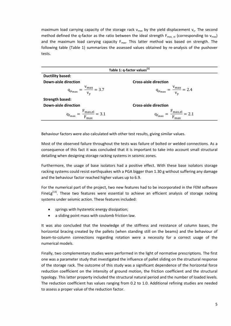
5

maximum load carrying capacity of the storage rack vmax by the yield displacement vy. The second

method defined the q-factor as the ratio between the ideal strength Fmax, el (corresponding to vmax)

and the maximum load carrying capacity Fmax. This latter method was based on strength. The

following table (Table 1) summarizes the assessed values obtained by re-analysis of the pushover

tests.

Table 1: q-factor values[1]

Ductility based:

Down-aisle direction Cross-aisle direction

Strength based:

Down-aisle direction Cross-aisle direction

Behaviour factors were also calculated with other test results, giving similar values.

Most of the observed failure throughout the tests was failure of bolted or welded connections. As a

consequence of this fact it was concluded that it is important to take into account small structural

detailing when designing storage racking systems in seismic zones.

Furthermore, the usage of base isolators had a positive effect. With these base isolators storage

racking systems could resist earthquakes with a PGA bigger than 1.30 g without suffering any damage

and the behaviour factor reached higher values up to 6.9.

For the numerical part of the project, two new features had to be incorporated in the FEM software

FineLg[13]. These two features were essential to achieve an efficient analysis of storage racking

systems under seismic action. These features included:

springs with hysteretic energy dissipation;

a sliding point mass with coulomb friction law.

It was also concluded that the knowledge of the stiffness and resistance of column bases, the

horizontal bracing created by the pallets (when standing still on the beams) and the behaviour of

beam-to-column connections regarding rotation were a necessity for a correct usage of the

numerical models.

Finally, two complementary studies were performed in the light of normative prescriptions. The first

one was a parameter study that investigated the influence of pallet sliding on the structural response

of the storage rack. The outcome of this study was a significant dependence of the horizontal force

reduction coefficient on the intensity of ground motion, the friction coefficient and the structural

typology. This latter property included the structural natural period and the number of loaded levels.

The reduction coefficient has values ranging from 0.2 to 1.0. Additional refining studies are needed

to assess a proper value of the reduction factor.

6

The second complementary study putted different types of seismic analyses next to each other.

These were:

the lateral force method;

a response spectrum analysis;

a pushover analysis.

The principal conclusion of this study was that all three methods resulted in similar test results,

provided that second order effects were accounted for in the specific method.

The SEISRACKS-project lead to a revised version of the draft normative document pr-FEM 10-2-08

"Recommendations for the design of static steel pallet racks under seismic conditions"[14].

As the first SEISRACKS-project was already successful, but more research was needed to get actual

design rules, the European Union launched a second project titled "Storage Racks in Seismic Areas 2"

in 2011. This project is still running and this dissertation is included in the project.

2.3 Seismic behaviour of racking systems in down-aisle direction

In this section, more detailed research is emphasized about the behaviour of steel storage racks in

the down-aisle or longitudinal direction. This behaviour is governed by two components of the

racking system. Primarily, the beam-to-column connectors have a big influence on the behaviour of

the storage rack, as failure of the rack is in general due to failure of these connectors. The second

component is the connection of the uprights with the floor level through a base plate. The rotational

stiffness of this base plate connection is an influencing factor for the longitudinal behaviour of the

storage rack. The rotational stiffness of both these entities is needed for achieving correct numerical

models. Halas, a lot of uncertainty still exists about achieving correct values for the stiffness of the

connectors.

2.3.1 The rotational stiffness of beam-to-column connectors

A lot of variety exists in the shape of the connectors, but also in the way they bring about the

connection between beam and column. In the United States and Australia for example, a bolted

connection is mainly used (Figure 1a) as where in Europe mostly a system of hooks and holes is used

that sometimes is secured by a bolt or spindle (Figure 1b).

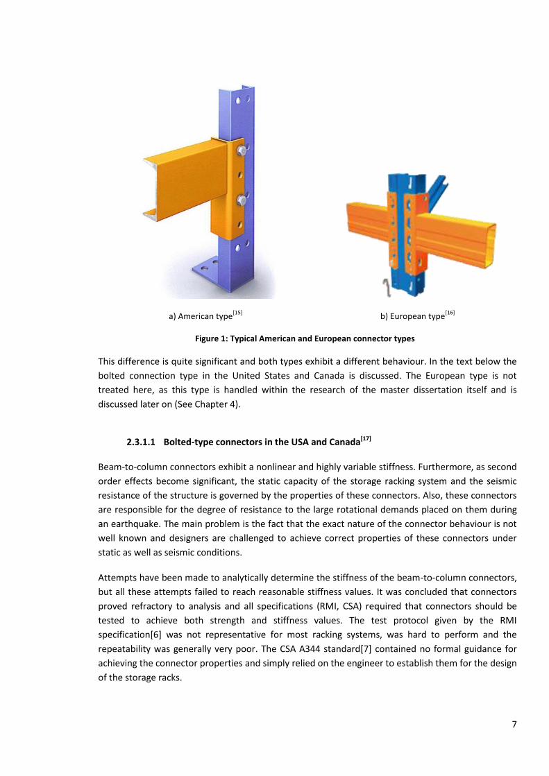
7

a) American type[15]

b) European type[16]

Figure 1: Typical American and European connector types

This difference is quite significant and both types exhibit a different behaviour. In the text below the

bolted connection type in the United States and Canada is discussed. The European type is not

treated here, as this type is handled within the research of the master dissertation itself and is

discussed later on (See Chapter 4).

2.3.1.1 Bolted-type connectors in the USA and Canada[17]

Beam-to-column connectors exhibit a nonlinear and highly variable stiffness. Furthermore, as second

order effects become significant, the static capacity of the storage racking system and the seismic

resistance of the structure is governed by the properties of these connectors. Also, these connectors

are responsible for the degree of resistance to the large rotational demands placed on them during

an earthquake. The main problem is the fact that the exact nature of the connector behaviour is not

well known and designers are challenged to achieve correct properties of these connectors under

static as well as seismic conditions.

Attempts have been made to analytically determine the stiffness of the beam-to-column connectors,

but all these attempts failed to reach reasonable stiffness values. It was concluded that connectors

proved refractory to analysis and all specifications (RMI, CSA) required that connectors should be

tested to achieve both strength and stiffness values. The test protocol given by the RMI

specification[6] was not representative for most racking systems, was hard to perform and the

repeatability was generally very poor. The CSA A344 standard[7] contained no formal guidance for

achieving the connector properties and simply relied on the engineer to establish them for the design

of the storage racks.

8

For stability design, beam-to-upright connections are typically modelled by a rotational spring

defined by a rotational spring constant k. In 1980 already, the need for this constant k was

recognized and values were recommended for computer modelling in the "Blume Report"[18]. But

these values were proven to be inaccurate. As a result of the problems stated above, there existed a

considerable uncertainty about the correct value of k for design purposes. In what follows below,

attempts to determine the quasi-static rotational stiffness of connectors and its variation with

movements caused by normal rack operations are illustrated. Also an attempt was made to achieve

stiffness values with increasing seismic demand.

Shake-table tests were conducted on four different storage rack specimens, made up of 2 bays and 4

levels (Figure 2).

Figure 2: Storage rack specimens[17]

The difference between the specimens was situated in different beam sizes with a specific type of

bolted beam-to-upright connectors. These four cases were as follows (see also Figure 3):

Rack 1: C4x4.5 beams, two-bolt hot-rolled connectors welded to the beam (Fig. 3a);

Rack 2: C5x6.7 beams, three-bolt hot-rolled connectors welded to the beam (Fig.3b);

Rack 3: e.g. Rack 1, but whole edges burred (Fig. 3c);

Rack 4: e.g. Rack 1, but connectors are cold formed (Fig. 3d).

9

a) b)

c) d)

Figure 3: Four different beam-to-upright connectors[17]

For further details about the storage rack specimens, reference is made to the article[17].

To simulate the pallet weight, standard concrete bricks were used to stack on the pallets. Each pallet

weighted 4.9 kN. The distribution of the pallets on the rack can be seen in Figure 2 above. For the

non seismic tests three different payloads were used:

The total pallet weight: 235 kN

66% of the total pallet weight: 157 kN

33% of the total pallet weight: 78 kN

For the seismic tests, the distribution of Figure 2 was used but the first level beams and pallet

weights were removed. This build-up carried a payload of 176 kN and the pallets were fastened to

the pallet beams in order to restrain pallet movement. In this way, the structural response of the

storage rack was more isolated.

A pull-back, white noise and seismic test was conducted on each specimen. For a description of these

tests, reference is made to the original article[17]. The purpose of the pull-back tests was to achieve

fundamental natural frequencies and damping characteristics of the rack specimens. With the white

noise tests, the variations of down-aisle dynamic properties was investigated. The objective of the

10

seismic tests was to determine the dynamic response of the four rack specimens subjected to strong

ground motions.

Also linear three-dimensional finite element models of the rack specimens were developed with SAP

2000[19]. With these models, the in-plane fundamental period as a function of the rotational stiffness

of the beam-to-upright connections could be predicted. These connections were modelled as

rotational springs and the payload on the pallet beams was modelled as lumped masses at each

level. For the base plates, the rotational stiffness was unknown. To overcome this problem, two

boundary conditions were applied for each model: a fixed base support and a pinned base support.

With these numerical models, period-rotational stiffness curves were generated for all payload cases

as seen in the figure below. (Figure 4).

Figure 4: Period - Rotational stiffness curve for rack models 1,3 and 4 with 33% payload[17]

When the rotational stiffness was larger than 500 kNm/rad, the base plate condition had a negligible

effect.

With the experiments, the fundamental period of the rack specimens was measured. This period was

then used in the curves like in the figure above to read off the range of average connector rotational

stiffness for each specimen. The figure below shows the results (Figure 5).

11

Figure 5: Estimation of average connector stiffness[17]

For a given rack specimen, values for connector stiffness seem relatively insensitive to variations in

content weight. The highest values are seen for Rack 2, which has the largest size beams and

connectors. Lowest values are seen for Rack 3.

With the results of the white noise tests, the variation of connector stiffness with excitation

amplitude could be estimated. The power spectral density of the top level acceleration time-history

was computed for each white noise test performed at a certain intensity (expressed in terms of RMS

acceleration). Then, two particular frequencies were achieved: the predominant frequency of the

response and the lowest frequency of the signal with an amplitude of at least 5% of the predominant

frequency amplitude. These frequencies or periods were used in the graphs like Figure 4 above to

estimate values for the connector stiffness for each white noise intensity. The result is given in Figure

6 for Rack 1. Similar graphs were made for the other three racks and can be consulted in the original

article. One sees that the connector stiffness reduces with RMS amplitude. This reduction was

estimated to be linear when the stiffness was logarithmically distributed in the graph.

After the completion of the white noise excitation, the free-vibration response was recorded and

proved that the initial connector stiffness was mainly recovered after the reduction during the white

noise test.

12

Figure 6: Results of the white noise test for Rack 1[17]

The results of the seismic test showed that the four rack specimens could undergo very large inelastic

deformations in the down-aisle direction without any significant loss of vertical load carrying

capacity. A second important result is illustrated in the figure below (Figure 7). This figure illustrates

the beneficial effects of the nonlinear characteristics of the connections: the rack structures are

isolated against large accelerations while the connectors also function as an additional source of

damping. This was proven with the fact that the acceleration did not vary linearly with height and for

three of the four racks, the absolute acceleration at the top was smaller than at the bottom of the

rack.

Figure 7: Peak absolute accelerations for most intense seismic tests[17]

13

2.3.2 Base plate stiffness[20]

The base plate stiffness is the second key property needed to achieve a successful numerical model.

Usually, a linear or nonlinear moment-rotation relationship is used to model the base plate

connection. There were two main ways to determine the base plate stiffness. The RMI Specification[6]

recommended an equation based on the dimensions of the base plate and the modulus of elasticity

of the floor. The European Standard EN 15512[11] on the other hand recommended testing for the

determination of the base plate stiffness. However, some inconsistencies were found in this test

setup and an alternative method similar to the European one was tested at the University of Sydney.

First, base plate behaviour is explained. Then, the European test setup is illustrated followed by the

alternative test setup and ways to attain stiffness values are given. Finally, the influence of the width

of the upright section on the stiffness is investigated.

2.3.2.1 Base plate behaviour

Base plates transmit axial forces and moments to the floor. Generally, the moment-rotation stiffness

and strength of base plate assemblies depend on the axial force that is exerted on the uprights. The

connection between the uprights and the base plate assembly is realized by bolts or by tabs, while

the connection between base plate and floor is usually done by bolting. A typical example of base

plate assemblies is given in the figure below (Figure 8).

Figure 8: Typical base plate assembly[20]

The deformation of a base plate system under an applied moment can be separated into four main

contributions, illustrated in the figure below (Figure 9):

Local deformation of the floor underneath the base plate (Fig. 9a);

Bending of the bracket of the base plate system (Fig. 9b);

Bending and rotation of the upright relative to the base plate assembly (Fig. 9c);

Formation of yield lines and flexure in the base plate (Fig. 9d).

14

a) b) c) d)

Figure 9: Four contributions to base plate deformation[20]

2.3.2.2 European and alternative test setup

According to EN 15512 Specification[11], a dual-actuator test arrangement is proposed (Figure 10). In

this test, two lengths of upright are symmetrically connected to a concrete block through base plate

assemblies. Two jacks are needed to apply an axial load in the upright and a lateral force on the

concrete block , inducing a moment in the base plate assembly. Also several transducers (LVDT's) are

placed to measure deformations. The precise position of these LVDT's is not specified, but to capture

all components of rotation over the length of the base plate assembly and not more, the optimal

position is located just above the bracket as shown in Figure 11.

a) plan view

b) side view

Figure 10: Dual-actuator test according to EN 15512[11]

Figure 11: Location of LVDT's[20]

15

At the beginning of the test, the axial load is increased to a desired level and kept constant during the

test. The lateral load is gradually increased until a maximum is reached. According to EN 15512[11],

the concrete block must be free to move in the horizontal plane, but has to be restrained from

rotating about its vertical axis. This last requirement is needed to ensure both base plates will fail

during the test. The inconsistency, according to Rasmussen and Gilbert[20], lies in the fact that a pin

connection is used between the concrete block and jack no. 2 (Figure 10a). Therefore, a slight

modification was done to the test setup proposed by EN 15512[11], shown in Figure 12. The concrete

block is connected to jack no. 2 using rigid plates and bolts in order to prevent its rotation. The holes

in the plate connected to the jack are slotted and the bolts are loosely tightened, giving the

availability of relative sliding between both plates so that the concrete block can move in a horizontal

plane. Jack no. 2 is laterally restrained as to prevent its rotation.

Figure 12: Plan view of alternative test setup[20]

Fifteen tests were performed with axial loads equal to 0, 33, 100, 150 and 200 kN at the University of

Sydney. The result of these tests is illustrated as a moment-rotation curve shown in the figure below

(Figure 13).

Figure 13: Moment-rotation curves for all tests[20]

16

Reference is made to the article for the calculation of moments and rotations out of the test

results[20]. (In fact, the formulas used were identical to those given in EN 15512[11]). For axial loads

greater than 100 kN, it is observed that the initial stiffness is almost the same. Due to looseness in

the system, initial rotations of the uprights were recorded when applying the axial load. To achieve

the curves to pass through the origin a shift on the horizontal axis was applied.

In the EN 15512 Specification[11], base plate stiffness values are calculated based on the characteristic

failure moment Mk, derived from the maximum moments Mti of several tests. It is stated that the test

must be run until jack no. 2 reaches a maximum load. However, test results have proven that the

load in jack no 2 can reach a maximum before large deformations have occurred in the base plate

and/or a maximum bending moment has been reached. Therefore, the point at which the lateral load

has reached its maximum is a bad indicator for when the maximum moment capacity is reached. In

the tests performed here, maximum bending moments were only achieved for the 150 and 200 kN

axial load tests. In the other three tests, the formation of plastic hinge lines in the base plate initiated

failure, but no maximum bending moment Mti was reached. So, an alternative way to get a maximum

moment was needed.

An ultimate deformation limit below which the base plate connection is not to fail was defined by

Kosteski and Packer[21]. Yura et al.[22] set this limit to four times the first yield deformation

(coefficients of 3 and 4 are generally used as indicators for whether a plastic hinge is able to occur

and sustain plastic deformations). Rasmussen and Gilbert[20] recommended this ultimate deformation

limit to be used as a criterion for determining the maximum moment Mti for base plate assemblies. In

the figure below, this method is illustrated for the 100 kN axial load test (Figure 14). The first yield

deformation is to find at the intersection between a line representing the elastic deformation and a

second one representing the plastic deformation.

Figure 14: Alternative method for achieving Mti[20]

17

2.3.2.3 Calculating values for base plate stiffness

As stated above, the RMI Specification[6] recommended equations to calculate the base plate

stiffness. The following expression was used:

With Mb the moment applied to the base plate, the base plate rotation, b and d the depth and

width of the upright section and Ec Young's modulus of the floor. This formula did not consider the

deformation of the base plate assembly itself and Sarawit[23] proposed two other formulae that

considered the properties of the concrete floor and the base plate geometry. For this case, the

following expression applied:

For the rotation of the upright itself occurring over the length of the base plate assembly, the

following expression was derived based on a single cantilever beam with a lateral point load F at the

top:

Where Eu is Young's modulus and Iu is the second moment of area of the upright section. L is twice

the length of the tested upright and a is the height above floor level where the LVDT's are placed to

measure the rotation of the base plate assembly. To account for both the deformation of the floor

and the rotation of the upright, a general stiffness constant can be obtained:

As is to see on the figure below (Figure 15), both kbu and ku give good approximations to the base

plate initial stiffness attained by experiment, especially for the high axial load tests. With this

observation it can be concluded that the initial deformation of the base plate assembly consists

generally of contributions shown in Figures 9a and 9c. Also, for serviceability limit state calculations,

kbu may be used for determining global serviceability deformations as deformations of the base plate

assembly stays in the elastic range.

For ultimate limit state design, Godley[24] proved that a certain value of base plate stiffness exists

beyond which there is no further increase in load carrying capacity of the racking system. This means

that the rack may be treated as fixed at the base. The stiffness corresponding to this limiting value is:

18

With Eu and Iu defined the same as above and h the distance from the floor to the first beam. In the

EN 15512 Specification[11], a bilinear procedure is specified to calculate design stiffness values for

every axial load. In the figure below (Figure 16), kh is plotted together with the k-values according to

EN 15512[11] and the test results. As kh is smaller than all other initial slopes, designing the rack with a

fully fixed base plate assembly will induce an accurate load carrying capacity of the racking system.

As a general conclusion, pre-design of storage racking systems can be done without experimental

test results, assuming a fixed-end condition at the bases.

Figure 15: Illustration of ku and kbu[20]

Figure 16: Illustration of kh and EN 15512 k-values[20]

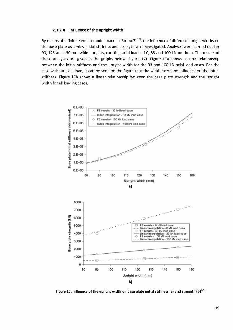
19

2.3.2.4 Influence of the upright width

By means of a finite element model made in 'Strand7'[25], the influence of different upright widths on

the base plate assembly initial stiffness and strength was investigated. Analyses were carried out for

90, 125 and 150 mm wide uprights, exerting axial loads of 0, 33 and 100 kN on them. The results of

these analyses are given in the graphs below (Figure 17). Figure 17a shows a cubic relationship

between the initial stiffness and the upright width for the 33 and 100 kN axial load cases. For the

case without axial load, it can be seen on the figure that the width exerts no influence on the initial

stiffness. Figure 17b shows a linear relationship between the base plate strength and the upright

width for all loading cases.

a)

b)

Figure 17: Influence of the upright width on base plate initial stiffness (a) and strength (b)[20]

20

2.4 FEM 10.2.08[2]

In this section, a summary is presented of the main specific features of the new recommendations

stated in FEM 10.2.08[2]. Before getting to the features, a short introduction is given about the

general context in which these recommendations are created. For the text below, reference is made

to a paper about FEM 10.2.08[26] and to the FEM recommendation itself[2].

2.4.1 Introduction

Racking systems are not regular buildings but a very particular form of steel construction. A lot of

differences exist between these two types of construction. Differences are to find in their use, the

loads that are supported (live load is bigger than dead load for storage racking systems), the

components used in their construction and the geometrical dimensions. Common components used

for storage racking systems are thin-gauge cold-formed profiles. In the case of uprights, these

profiles are continuously perforated with the purpose to achieve the required functionality,

adaptability and flexibility to cope with the great variation in goods to be stored. While national

building seismic regulations give design approaches for ordinary steel structures, it is of great

importance to define whether it is possible to apply these 'general design rules' to steel storage

racks. Furthermore, it is of great importance to consider how to modify these general principles and

technical requirements correctly in order to take into account the peculiarities of storage racks and

to achieve the requested safety level.

To give an answer to these problems, a working group was initiated by the European Racking

Federation (ERF) a few years ago. The main result of this group was a new Code of Practice issued in

September 2010 titled FEM 10.2.08[2]. In January 2011, the ERF working group transformed into a

CEN working group. The purpose of this 'new' working group was to transpose the Code of Practice

into a European Standard EN.

2.4.2 Fundamental requirements

The Code of Practice FEM 10.2.08 considers three levels of fundamental requirements[26]:

No collapse requirement;

Damage limit state requirement;

Movement of unit loads.

The 'No collapse requirement' corresponds to the classical requirement of EN 1998-1[3] that states

that no local or global collapse during the earthquake is tolerated and that after the earthquake, a

sufficient structural integrity and residual load bearing capacity of the structure is present. This

requirement is based on verification of resistance and ductility, including the resistance of the

bracing system if present, as well as the check of a 'no collision' criterion between unconnected

racks or between racks and adjacent structures.

21

For the 'Damage limit state requirement', no specific damage requirements are prescribed by FEM

10.2.08[2] at the design stage. The damage limitation requirement foreseen in EN 1998-1[3] is

replaced by a compulsory assessment of the damage caused by the earthquake for all seismic

events with PGA higher than 50% of the design PGA to be considered for no collapse requirements.

The 'Movement of unit loads' section is added because experience has shown that stored goods are

likely to exhibit significant movements during a seismic event, in particular sliding and/or rocking. It

is important that the client is informed about the risk related to this unit load movement, as the

stored goods can fall from the rack. This has to be done considering the working conditions of the

warehouse.

The reference return period of the design earthquake as it is defined in EN 1998-1[3] is managed

through an importance factor scaling the design spectrum. The reference value of 1.0

corresponds to a return period of 475 years, meaning a probability of exceedance of 10% for a

reference period of 50 years. For rack structures, the reference period is commonly reduced to 30

years. This leads to reduced values of the importance factor. Furthermore, importance classes have

been established for racks giving proper importance factors. These classes are the following:

Class I: Warehouses with fully automated storage operation or with low occupancy;

Class II: Standard warehouse conditions;

Class III: Retail areas with public access;

Class IV: Hazardous product storage.

2.4.3 Design spectrum - coefficients ED1, ED2 and ED3

In FEM 10.2.08[2], no recommendation is made on the definition of the reference elastic response

spectrum in terms of shape and ground acceleration. Reference is made to EN 1998-1[3] or to the

appropriate national annexes or standards. The only difference for storage racking systems is the

value of structural damping. On the base of experimental evidence, this value is recommended to be

3% instead of 5%. Furthermore, it is noted that the elastic spectrum is not used for design actually,

but used for assessing the sliding and rocking behaviour of stored goods. For design purposes, the

Code of Practice uses the same definition of the spectrum as stated in EN 1998-1[3] (See also Chapter

6 of this dissertation). For usage of this design spectrum in the case of storage racking

systems, FEM 10.2.08 introduces two reduction factors, leading to an adapted design spectrum for

practical use[2]:

The corrective factor is introduced to account for energy dissipation through friction between

pallets and rack beams. The factor is computed according to the equation below.

This equation was calibrated on the base of a theoretical model assuming that pallets behave as

point masses sliding on the rack and depends on:

22

The intensity of the seismic action;

The dynamic characteristic of the structures;

The friction properties of the contact between pallet and beam.

When pallets are blocked on the beams, no energy dissipation through sliding can occur and the

coefficient is set equal to 1.0. For proper evaluation of this coefficient, the knowledge of the friction

properties of the contact between pallets and beams is necessary. FEM 10.2.08[2] recommends

reference values for pallet-beam friction coefficients for different types of materials in contact.

Moreover, safety factors are given that shall be applied on the reference values prior to its use in the

equation above.

The second corrective factor is introduced to account for other phenomena typical for the

dynamic behaviour of racking structures under seismic action that are not incorporated in the model

giving rise to factor . These phenomena were observed on racks that have experienced

earthquakes and in shake table tests. According to FEM 10.2.08[2], the recommended value is equal

to 0.667.

To account for the effects of the dynamic interaction between pallet and racking structure and for

the possibility to dissipate seismic energy in the stored goods themselves, a third and final corrective

factor is created called the weight modification factor. Its main influence is focused on the

response to seismic action in terms of participating mass. This factor depends on the type of

palletized goods. To evaluate the horizontal seismic action in practice, the design pallet weight to be

considered is calculated as follows:

with:

: the rack filling reduction factor;

: the maximum weight of the unit loads

FEM 10.2.08[2] recommends values for .

2.4.4 Structural analysis - second order effects

The Code of Practice provides specific information on how to proceed with the structural analysis of

storage racking systems. Two main aspects are treated, the first being related to the modeling

assumptions and the second to methods of analysis.

2.4.4.1 Modeling assumptions

Information is given about:

The conditions under which the analysis can be carried out on separate substructures rather

than on the entire racking system;

23

The loading model (arrangement of masses), including conditions for the verification of the

uplift at the upright bases;

The way to account for possible eccentricity of the gravity centre of the pallets with respect

to their supporting beams in the case of differential loading of the pallet beams for cross-

aisle analysis and of additional compression loading of the uprights for down-aisle analysis of

racks with limited number of spans (Figure 18);

The stiffness properties of the structural elements to be considered for seismic analysis.

Appropriate reference is made to standardized mechanical characterization given in EN

15512 (Standard for static design)[11];

Analysis of the pallet beams:

o On the calculation and combination of internal forces (axial force, horizontal and

vertical bending);

o On the calculation of the buckling length in both the vertical and horizontal plane. In

the vertical plane, the contribution of the beam-to-column connection stiffness is

accounted for. In the horizontal plane, the restraining effect exerted by the pallets is

incorporated (in accordance with the occupancy of the rack)

a) Cross-aisle behaviour

b) Down-aisle behaviour

Figure 18: Eccentricity of the gravity centre[2]

24

2.4.4.2 Methods of analysis

In FEM 10.2.08[2], the fundamental methods of analysis stated in EN 1998-1[3] are recalled. The

fundamental methods are the Lateral Force Method of Analysis (LFMA) and the Modal Response

Spectrum Analysis (MRSA). Furthermore, some implications of the use of these fundamental

methods for storage rack analysis is given, including the conditions under which LFMA can be

replaced by MRSA, considered as the reference method. Also a nonlinear equivalent static analysis

called the Large Displacement Method of Analysis (LDMA) is proposed. This latter method forms an

alternative to the classical pushover analysis described in Annex B of EN 1998-1[3].

Storage racking systems are highly sensitive to geometric second-order effects. This feature is

measured by the Inter-storey Drift Sensitivity Coefficient . This method is also recommended by En

1998-1[3]. The coefficient is defined as:

with:

: the total gravity load at the considered level;

: the total seismic storey shear at the considered level;

: the design inter-storey drift;

: the inter-storey height.

An alternative definition of the Inter-storey Drift Sensitivity Coefficient is also given. In this definition,

the sensitivity factor depends on the behaviour factor and on the Euler critical load. The latter is a

common result from static analysis of storage racks.

In FEM 10.2.08[2], requirements are given in terms of the method of analysis and of the allowed

approach to incorporate second order effects. These requirements are based on the value of the

sensitivity factor stated above and on the chosen design concept (i.e. low dissipative or dissipative).

In the figure below, a summary of these requirements are given (Figure 19). Important to mention

here is that the transition values of are less conservative than those proposed in EN 1998-1[3].

Figure 19: methods of analysis

[2]

25

2.4.5 Design concepts - behaviour factors

According to FEM 10.2.08, the design of earthquake resistant racks is performed through one of the

following concepts[2]:

Low dissipative structural behaviour;

Dissipative structural behaviour.

The concept of low dissipative structural behaviour means that the effects of seismic actions are

computed by means of elastic global analysis. No relevant nonlinear behaviour is taken into account.

With the dissipative concept, plastic deformation can occur in certain zones of the structure. These

zones are called dissipative zones. The capacity of plastic deformation is defined by the behaviour

factor q. In contrast with En 1998-1[3], there's no distinction between Ductility Class Medium and

High (DCM and DCH) design concepts.

The behaviour factor depends on the regularity of the structure, the classification of the members'

cross section and on the structural type of the structure. For determining regularity, FEM 10.2.08[2]

defines regularity criteria that are suitable for the assessment of classical rack configurations (i.e.

mass and stiffness regularity in horizontal and vertical plane for cross- and down-aisle direction).

To achieve behaviour factors for the upright frames (cross-aisle direction), several possible bracing

arrangements are considered. These are shown in Figure 20 below. For each of these arrangements,

a specific design procedure is given (i.e. dissipative design allowed or not, safety factors for

connections, maximum behaviour factor).

Figure 20: possible bracing arrangements

[2]

26

To achieve q-factors in the down-aisle direction, difference is made between two structural types:

Moment resisting frames;

Frames with concentric vertical bracings.

In the case of moment resisting frames, horizontal seismic forces are resisted by the flexural

behaviour of members and connections. The behaviour factor is taken to be 1.5 to 2.0 for low

dissipative concept. The value of 2.0 is associated with limited additional requirements such as the

utilisation of a bolt to secure beam-to-column connections.

For both types of configurations, the maximum allowed values of the behaviour factors in case of

dissipative design are the same values as in EN 1998-1[3] for DCM design concept (for similar

structural types).

Moreover, this Code of Practice provides the design rules that must be followed for low dissipative

and dissipative structures, with respect to the required material properties, the connection

properties and the cross-section classification.

Finally, a specific chapter dedicated to detailing rules for dissipative elements is included in FEM

10.2.08[2]. This chapter is only to be used when the dissipative design concept is followed. It includes

consideration for:

Capacity design of connections in case plastic dissipation occurs in the members;

In the case of moment resisting frames, strength and ductility requirements for connections

when the structure is designed such that the dissipative zones are located in the

connections. Also, associated capacity design rules for the uprights and beams are given.

Requirements for dissipative design of concentrically braced frames, where energy

dissipation is located in the tension diagonals or in the connection of these diagonals.

Capacity design rules for the horizontal bracings, provided that they contribute to the

earthquake resistant structural system, in particular for racks that are vertically braced in the

rear plane.

2.4.6 Additional information

A set of annexes providing additional information including references to external background

documents is incorporated in FEM 10.2.08[2]. The most significant ones are summarized below.

Annex B lists the minimum design data that is to be provided by the Specifier/End User of the

installation. Basic design conditions, interaction with the building floor, pallet and product

specifications and building clearances are met in the data set. A typical layout of datasheet

for the gathering of all information is proposed;

Annex C provides a test procedure for the determination of the pallet-beam friction

coefficient, in case the designer or user wants to obtain reliable values for its specific

products. Also a methodology for processing the test results is included;

Annex D deals with the assessment and prevention of rocking of palletized goods;

27

Annex E states the background considerations and modelling assumptions that were

established to create the equation for computing ;

Annex F summarizes technical solutions to prevent pallets from falling due to excessive

sliding motion;

Annex G illustrates the experimental characterization of the properties of beam-to-column

connections. Requirements for the loading history are given and failure criteria that shall be

applied in the cyclic testing of beam-end connectors when dissipative design implying a due

control of the connection behaviour is used, are provided.

28

3. SEISRACKS 2

In this chapter, more information of the project "Storage racks in seismic areas 2" is given. First an

overall overview of the project is given, i.e. the goal of the project, the participating units, ... . This is

followed by a short section situating this dissertation in the project and illustrating the purpose and

use of this dissertation.

3.1 Storage racks in seismic areas 2

As said in the former section about FEM 10.2.08, a CEN working group is currently developing a

preliminary normative document based on FEM 10.2.08[2] and on the base of recent research works.

However, the documents are still far from becoming an Euronorm EN. The main reasons for this are

the remaining lacks of knowledge, leading to conservative design rules. As a consequence of these

conservative approaches, technical limitations arise when designing static steel storage racking

systems with respect to seismic safety. The main objective of the SEISRACKS 2 project is to get rid of

these limitations by increasing the knowledge on actual structural behaviour and ductility.

Furthermore, full-scale testing and numerical simulation is performed through the project to achieve

design rules for earthquake conditions.

The main expected outcomes of the research project are:

Detailed reports on the different aspects investigated;

Evaluation of the current draft of FEM 10.2.08[14] and validating the incorporated rules;

Achieving improvements and extension of the current rules, so that the seismic behaviour of

structures designed according to European rules is optimized;

The definition of standardized experimental procedures for the qualification of structural

elements of storage racking systems to be used in seismic areas;

The development of a software tool in order to design rack structures in seismic active

zones.

The participators in the project are companies as well as academic institutions:

Universities:

Politecnico di Milano;

National technical university of Athens;

Rheinisch-Westfaelische technische hochschule Aachen;

Université de Liège.

Companies:

SCL INGEGNERIA STRUTTURALE;

NEDCON Magazijninrichting B.V.;

MODULBLOK S.p.A.;

29

STOW INTERNATIONAL nv;

FRITZ SCHÄFER GmbH;

COMPUTER CONTROL SYSTEMS S.A.

3.1.1 Work Packages and tasks

As was the case in the first SEISRACKS project[1], the work to be done is subdivided in work packages.

Below, all work packages for SEISRACKS 2 are listed together with the subdivision in tasks.

WP 1: Definition of case-studies;

o Task 1.1: Identification of weaknesses in FEM 10.2.08[2] and comparison with RMI[6];

o Task 1.2: Definition of typical structural typologies;

o Task 1.3: Design of case studies.

WP 2: Component testing;

o Task 2.1: Tests on beam-to-column connections;

o Task 2.2: Tests on column bases;

o Task 2.3: Tests on substructures;

o Task 2.4: Calibration of the components method for rack connection

characterization.

WP 3: Warehouse testing;

o Task 3.1: Continuous monitoring of an installation;

o Task 3.2: Identification of racks' dynamic properties;

o Task 3.3: Identification of merchandizes' dynamic properties.

WP 4: Full scale testing;

o Task 4.1: Definition of test structures and of testing procedures;

o Task 4.2: Execution of tests.

WP 5: Numerical analyses;

o Task 5.1: Classical analyses at design stage;

o Task 5.2: Post-test calibration of numerical models;

o Task 5.3: Parameter study on structural behaviour;

o Task 5.4: Parameter study on merchandize-structure interaction.

WP 6: Assessment of seismic design methodology;

o Task 6.1: Assessment of q-factors;

o Task 6.2: Assessment of Qp and Rf factors;

o Task 6.3: Assessment of Ed1 and Ed2;

o Task 6.4: Assessment of methods of analysis;

o Task 6.5: Development of qualification testing for structural components;

o Task 6.6: Drafting of Designer's Manual.

WP 7: Software tool development;

o Task 7.1: Theoretical analysis of the design method;

o Task 7.2: Software components development;

o Task 7.3: Introduction of the software components in driver software;

o Task 7.4: Parametric study for the calibration of the proposed procedure.

WP 8: Coordination.

30

For each work package, several institutions are responsible for completing the tasks.

The SEISRACKS 2-project was launched in July 2011 and at the time of writing, the project is halfway.

In what follows, a summary of the work done in the first mid-term of the project is given.

Furthermore, an overview of the work that has to be done in the following years is presented.

3.1.2 Mid-term summary

Up till now, the following work has been undertaken:

Identification of weaknesses in FEM 10.2.08[2] and comparison with RMI[6] (WP 1);

Definition of design parameters and geometrical properties to be used in the tests and

numerical analyses (WP 1);

Production of case studies to be used in the tests and numerical analyses. This was done by

the industrial partners (WP 1);

Component tests on beam-to-column connectors in cross- and down-aisle direction (See also

Chapter 4). In addition to the test program included in the proposal, pallet friction tests have

been done to allow for the determination of the influence of pallets on the resistance in the

cross-aisle direction. Column base tests are running at the time of writing (WP 2);

Substructure tests have been initiated. Numerical analyses for these test scenarios are

already developed, to be calibrated later on (WP 2);

Monitoring activities of existing installations in warehouses have been started (WP 3);

Definition of full scale testing conditions and selection of structures to be tested. The testing

itself has been delayed due to administrative problems (WP 4);

Development of numerical models for eight case studies. This was done according to the

daily practice using conventional analysis methods and recommendations of FEM[2] (WP 5).

Development of the software tool has been initiated. The theoretical analysis of the design

method has been completed (WP 7).

3.1.3 Future work

In the years to follow, the following work has to be initiated and/or completed:

Component testing (WP 2);

Warehouse monitoring (WP 3);

Full scale tests (WP 4);

Calibration of numerical models depending on the results of the tests (WP 5);

Assessment of seismic design methodology, development of seismic design rules, revision of

FEM 10.2.08[2], preparation of standard testing procedures for the qualification of joints and

substructures. This is done by following and achieving results from WP 1 to WP 5 (WP 6);

Development of a Designers' manual for seismic design of racks according to FEM[2] and new

rules achieved from this research program (WP 6);

Finalizing the development of the new software tool (WP 7).

The SEISRACKS 2 project is planned to be terminated in July 2014.

31

3.2 Purpose and situation of the dissertation

This dissertation takes part in the tasks that were assigned to the University of Liège, more

specifically, it takes part in Work Package 5. The main purpose of this dissertation is to give a solution

to the following problem:

When design of storage racking systems has to be performed using experimental analysis, this

experimental analysis on large racking structures cannot always be performed because of the lack of

experimental equipment at this large scale (i.e. shake floor tests for complete storage racking

systems with dimensions of tenths of meters in length and/or width).

The solution to this problem is to create a numerical model in specialized software that simulates the

behaviour of storage racking systems as realistic as possible. This numerical model can serve as an

alternative to the (commonly expensive) experimental tests that are required in design

recommendations.

The goal of this dissertation is to achieve consistent and realistic behaviour characteristics of large

storage racking systems exposed to seismic action in the down-aisle direction by examining small

units of these racking systems. This is achieved by establishing two-dimensional numerical models in

the down-aisle direction for the four producers participating in this project, making use of the

software package FineLg. Evaluation of the overall behaviour as well as comparison between the

products is performed.

In a next stage of the SEISRACKS 2 project, the results of this dissertation will be compared with

results of experimental tests of the real storage racking structures of the producers. This comparison

will result, in an ideal situation, to rules that will describe the extrapolation of the storage rack

behaviour resulting from numerical testing to the real storage rack behaviour under seismic loading.

To be able to establish these numerical models, use is made of the test results of the experiments

that were conducted at the RWTH Aachen Stahlbau University within the SEISRACKS 2 project.

Furthermore, design sheets adopted from each producer and some sections of the final report of the

SEISRACKS project[1] are used.

Finally, because of confidentiality reasons, the four producers stated here are not mentioned by

name in the further text of this dissertation. For the chapters to follow, the four producers will be

mentioned using letters, i.e. Producer A, Producer B, Producer C and Producer D.

32

4. Experimental component tests

According to the schedule of the SEISRACKS 2 project, the RWTH Aachen Stahlbau University had to

conduct the following tests (Work Package 2):

Tests on column bases to evaluate the rotation stiffness and strength;

Tests on beam-to-column connectors to evaluate rotation stiffness and strength.

The results of such tests are necessary to establish accurate numerical models as the beam-to-

column connectors and column base connections are modelled as rotation springs. In this

dissertation, numerical 2D models were established in the down-aisle direction. So, values for the

rotation spring stiffness and strength were needed in this direction. In what follows, the beam-to-

column connector tests and the column base tests in the down-aisle direction are discussed.

4.1 Beam-to-column connector tests in down-aisle direction

As is said above, beam-to-column connectors are commonly modelled as rotation springs in

numerical models and experimental testing is needed to achieve values for rotation spring stiffness

and strength. These spring characteristics are achieved by performing monotonic pushover tests. The

result of such a test is a moment-rotation diagram. This diagram illustrates the whole connector

behaviour during the test. Furthermore, cyclic tests were performed from which the energy

dissipating behaviour of the connectors can be evaluated. For both tests, the influence of the

payload is evaluated by interpreting the moment-rotation curves. For the text to follow, reference is

made to the report established by the University of Aachen[27].

4.1.1 Test setup

On the figure below, the overall test setup is illustrated (Figure 21). Two columns and one beam were

connected to each other by two connectors, that were welded to the beam. The connection with the

columns was done in a manner that was unique for each product. This system was incorporated in a

total frame that was necessary for its overall stability (falling in transverse direction, uplift,...). The

stability frame was put together so that every connection was hinged. In this way, no load was taken

by other connections than the connections of the test frame. This total frame was also necessary to

carry the payload. A hydraulic jack was then mounted onto a stiff frame in the laboratory on one side

and to a beam incorporated in the system on the other side. The stiff frame restrained any

displacement of the outer end of the hydraulic jack, so that the total force was exerted on the test

frame. The beam, connected to the hydraulic jack, was attached to both columns of the test frame.

With this attachment, the same displacement was exerted on both columns. The base plates of each

column were mounted on a metal box that contained sufficient space for the installation of

measuring devices.

33

The length of the pallet beam was 2,70 m (this is a sufficient and common length to carry three

payload pallets, put next to each other). The columns had a height of approximately 1 m. The pallet

beam was connected to the columns at approximately half of this height.

The payload existed out of three pallets, each pallet carrying a maximum of 800 kg when the fully

loaded condition was tested. Also a half loaded and an unloaded condition was incorporated in the

tests. For the half loaded tests, each pallet carried 400 kg of payload and for the unloaded tests no

pallets were placed on the beams. For safety reasons, a lifting device was used to put the payload on

the pallet beams and this device stayed under the pallets (no contact) so that the payload wouldn't

fall on the ground when the test setup failed.

Figure 21 : Test setup for connector testing in down-aisle direction[27]

The figure below shows a photograph of the test setup (Figure 22).

Figure 22 : photograph of the test setup[27]

As was stated above, three different payload cases were tested for each product:

Fully loaded case: each pallet carried a mass of 800 kg;

Half-loaded case: each pallet carried a mass of 400 kg;

Unloaded case: no payload was exerted on the beams.

34

All four producers supplied the products to be tested. The selection of sections was made by the

producers according to their experience. Only for product B, an earthquake bolt was incorporated in

the assembly. The other three products were assembled with the obligatory safety pin. The figure

below shows the products that were tested (Figure 23).

Figure 23 : types of products tested[27]

4.1.1.1 Measuring devices

In this test setup, devices were used to measure force and displacement. on the figure below, an

overview of all testing devices is given (Figure 24).

For a start, the applied force and displacements by the hydraulic jack were measured. For the

displacement, this measurement was done for the front beam as well as the backside beam. Second,

top and bottom displacement were evaluated at the left and right connection. For this measurement,

four devices were needed, two for each connection. Finally, two forces were measured at the bottom

of each column. So, four force measuring devices were needed from which two were needed for

horizontal forces and the other two for vertical forces.

With all these devices, an accurate test could be performed and the right data collected to perform

an analysis that resulted in force-displacement graphs, moment-rotation graphs and energy

consumption characteristics.

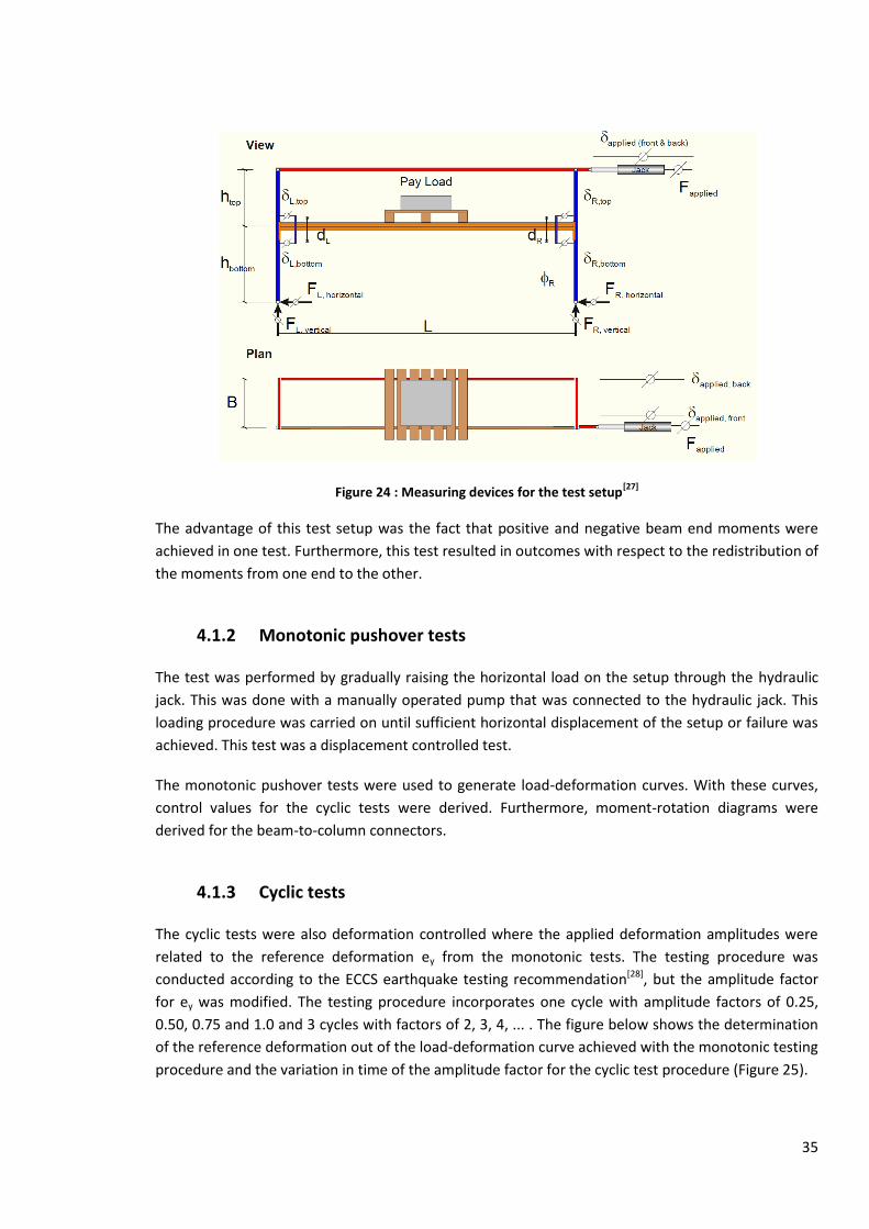
35

Figure 24 : Measuring devices for the test setup[27]

The advantage of this test setup was the fact that positive and negative beam end moments were

achieved in one test. Furthermore, this test resulted in outcomes with respect to the redistribution of

the moments from one end to the other.

4.1.2 Monotonic pushover tests

The test was performed by gradually raising the horizontal load on the setup through the hydraulic

jack. This was done with a manually operated pump that was connected to the hydraulic jack. This

loading procedure was carried on until sufficient horizontal displacement of the setup or failure was

achieved. This test was a displacement controlled test.

The monotonic pushover tests were used to generate load-deformation curves. With these curves,

control values for the cyclic tests were derived. Furthermore, moment-rotation diagrams were

derived for the beam-to-column connectors.

4.1.3 Cyclic tests

The cyclic tests were also deformation controlled where the applied deformation amplitudes were

related to the reference deformation ey from the monotonic tests. The testing procedure was

conducted according to the ECCS earthquake testing recommendation[28], but the amplitude factor

for ey was modified. The testing procedure incorporates one cycle with amplitude factors of 0.25,

0.50, 0.75 and 1.0 and 3 cycles with factors of 2, 3, 4, ... . The figure below shows the determination

of the reference deformation out of the load-deformation curve achieved with the monotonic testing

procedure and the variation in time of the amplitude factor for the cyclic test procedure (Figure 25).

36

Figure 25 : determination of ey (left) and variation in time of the amplitude multiplier (right)[27]

The results of the cyclic test were translated in moment-rotation curves for the beam-to-column

connectors.

4.1.4 Test results

In this section, the results of both tests are summarized. First, the failure modes are defined. Second,

the influence of the payload on the structure is evaluated. Third, a comparison is made between the

monotonic and cyclic behaviour of the test setup. Fourth, the moment-rotation characteristics are

illustrated. Finally, the effect of earthquake bolts on the earthquake resistance is evaluated.

4.1.4.1 Failure modes

Two main failure modes were observed during the testing:

Beam failure:

Cracks and/or buckles were observed at the beam ends and no or minor deformation of the

hooks of the connector and holes of the column was seen;

Connector failure:

Large deformation was observed at the hooks of the connector and/or holes of the column.

No or minor deformation was seen at the beam ends.

Either one or both of these failure modes (one failure mode for each beam end) were observed in

one test. The failure mode had an important influence on the degradation of the resistance of the

system. An illustration of the failure modes for the four products achieved during the monotonic

testing procedure is shown in the figure below (Figure 26).

37

Figure 26 : Failure modes during monotonic test procedure[27]

4.1.4.2 Influence of the payload

As stated above, three cases of payload were examined. From the tests, it can be concluded that the

payload has a significant positive influence on the resistance of the system, while the stiffness of the

system in the elastic range seems to be independent from loading. The main reason why the

resistance is growing with payload is that the hooks make a better connection with the column at the

holes due to the vertical load and more force is transferred between beam and column. The findings

stated here are illustrated in the figure below for all products (Figure 27).

Figure 27 : Load-displacement curves for the four products[27]

38

4.1.4.3 Comparison of cyclic and monotonic tests

By comparing cyclic and monotonic tests, the degradation of the resistance of the system can be

evaluated. The bigger the distance of the curves, the bigger the degradation of the resistance. From

this approach, the systems with connector failure seem to have an advantage compared to those

with beam failure. But, the load level of systems resulting in beam failure is significantly higher than

those ending up in connector failure. In the figure below, the comparison of cyclic and monotonic

tests is illustrated for all products for the fully loaded case (Figure 28).

Figure 28 : Comparison of cyclic and monotonic curves for the fully loaded case[27]

4.1.4.4 Moment-rotation characteristics

The moment-rotation curves were derived from the measured forces and displacements during the

tests. Two different moments were calculated to account for the influence of the payload:

Mpush : the moment due to horizontal loading of the frame;

Mtotal : the sum of moments due to horizontal loading and the payload.

Positive moments were defined as sagging moments and negative moments as hogging moments.

The figures below show the moment-rotation curves for the push moment and the total moment

respectively, for the monotonic tests (Figures 29 and 30).

39

Figure 29 : Monotonic push moment-rotation curves[27]

On the curves above, it can be seen that the resistance of the rack against lateral deflection is

practically independent from the payload applied on the pallet beams. The curves for the different

payloads almost overlap for each product. Especially in the elastic range, the initial stiffness of the

beam-to-column connectors can be assumed to have the same value for the three payload cases.

This observation has significant importance, as simplifications are possible for design on the basis of

moment-rotation curves. The black dashed curves are the design curves, received from the

producers.

Furthermore, the curves above show that the resistance moments in all tests reached the design

resistance:

For the design on the basis of moment-rotation curves, this fact also means that significant

simplifications are possible.

In this dissertation, these curves were used to implement the rotation spring characteristics for the

beam-to-column connectors in the numerical models. In the text below, a table is given with ranges

of initial stiffness values for the beam-to-columns connectors of the four products (Table 2). This

table was used to define average initial stiffness values for the connector rotation springs in the 2D

models when nonlinear analyses using a piecewise function to define the rotation spring

characteristics, were performed (See Chapter 5).

40

Figure 30 : Monotonic total moment-rotation curves[27]

For the total moment-rotation diagrams, it is observed that in the half-loaded and fully loaded cases

the curve is shifted downwards. Obviously, this means that the payload exerts an additive moment

with the push moment on the left side connector and a subtracting moment with the push moment

on the right side connector. It was also observed during the tests, that the initial moment due to the

payload was susceptible of the order in which the pallets were placed onto the beam.

For the cyclic tests, comparison was made with the curve envelopes as the amount of cycles in the

complete diagrams was excessively big and the conclusions made would be illustrated unclear in the

figures. The figure below shows the push moment-rotation curve envelopes for the four products

and the three payload cases (Figure 31). On these diagrams, it can be seen that the payload has no

significant influence on the moment resistance of the beam-to-column connectors as the curves for

the different payload cases nearly overlap each other. This was also the case in the monotonic tests.

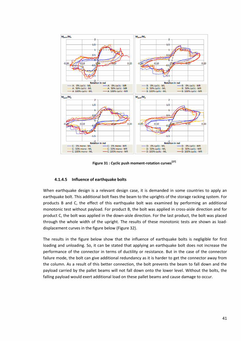
41

Figure 31 : Cyclic push moment-rotation curves[27]

4.1.4.5 Influence of earthquake bolts

When earthquake design is a relevant design case, it is demanded in some countries to apply an

earthquake bolt. This additional bolt fixes the beam to the uprights of the storage racking system. For

products B and C, the effect of this earthquake bolt was examined by performing an additional

monotonic test without payload. For product B, the bolt was applied in cross-aisle direction and for

product C, the bolt was applied in the down-aisle direction. For the last product, the bolt was placed

through the whole width of the upright. The results of these monotonic tests are shown as load-

displacement curves in the figure below (Figure 32).

The results in the figure below show that the influence of earthquake bolts is negligible for first

loading and unloading. So, it can be stated that applying an earthquake bolt does not increase the

performance of the connector in terms of ductility or resistance. But in the case of the connector

failure mode, the bolt can give additional redundancy as it is harder to get the connector away from

the column. As a result of this better connection, the bolt prevents the beam to fall down and the

payload carried by the pallet beams will not fall down onto the lower level. Without the bolts, the

falling payload would exert additional load on these pallet beams and cause damage to occur.

42

Figure 32 : Influence of earthquake bolts[27]

4.1.5 Comparison with bolted-type connectors

In this section, a short comparison is performed between the test results achieved here and the test

results for bolted-type connectors achieved from tests performed in the United States. These test

results were also mentioned in chapter 2 "Literature study" of this dissertation under subtitle

"2.3.1.1 Bolted type connectors in the USA and Canada". From this text, Figure 5 is illustrated a

second time below (Figure 5).

In this figure, a range of initial beam-to-upright average connector stiffness is given for different rack

systems. These values can be compared with the values achieved from the test results from the

experiments conducted in Aachen. In the table below, ranges of values for the initial stiffness of

beam-to-column connectors for the four products are summarized. The range is obtained by

different kinds of analysis (Table 2).

For the stiffness values given in Figure 5, a significant amount of overlap of the ranges can be noted

for different percentages of payload. This is also the case for the stiffness values given in the table. So

it can be concluded that the payload does not exert a significant influence on the initial connector

stiffness (See Table 2 ). The main conclusion when comparing the values in the table with the values

from the figure is that the initial stiffness for bolted connectors (figure) is significantly higher than the

stiffness values for hooked-in connectors (table). Thus, connectors that are bolted to the columns

have a higher stiffness than the connectors that are 'hooked' into the columns. This statement is

logical because a bolted connection itself is certainly more stiff than just putting hooks into holes.

43

Table 2 : initial stiffness values for beam-to-column connectors[27]

Product Payload (%) Initial stiffness (kNm/rad) A 0 82-100 50 62-120 100 68-110

B 0 200-240 50 180-240 100 180-230

C 0 88-140 50 100-180 100 112-177

D 0 88-102 50 76-124 100 120-140

Figure 5: Estimation of average connector stiffness[17]

44

4.2 Column base tests in down-aisle direction

Column base tests are also to be performed. These tests are performed to achieve moment-rotation

characteristics of the connection between column and base plate. The connection of the base plate

to the floor is not within the scope of these tests. Similar to the beam-to-column connector tests,

these tests result in moment-rotation curves. The moment-rotation curves are used to define

moment-rotation characteristics of the connection. Furthermore, these characteristics can be used

as rotation spring characteristics in numerical models like those used in this dissertation, as the

column base connections, like the beam-to-column connectors, are modelled as rotation springs in

the down-aisle direction.

As the column base tests only started running at the time of writing, the results could not be used for

the numerical analyses performed for this dissertation. As no results are available at the moment,

only a brief illustration about the proposed test setup and the testing procedure is given in the text

below. Reference is made to the test report for more information[29].

4.2.1 Test setup

The proposed test setup for the column base tests is shown in the figure below (Figure 33).

Figure 33: Test setup for column base tests[29]

A column base is rigidly connected to the underground that exists out of a rigid steel plate. On top of

the upright, a steel plate is mounted that is necessary for the connection with the vertical pendulum

and also the horizontal load will be applied at this level. The pendulum is pin connected on both its

sides and is incorporated in the setup to allow the upright top level to deflect horizontally. A vertical

45

hydraulic jack is connected to the pendulum to apply axial load onto the upright. The axial load is

controlled to be constant during the test, so the loading is force controlled. The horizontal load is

also established by a hydraulic jack, but this jack is displacement controlled. In this test, the applied

horizontal force is measured for a given displacement and also horizontal forces from second order

effects are measured by horizontal devices.

4.2.2 Testing procedure

The figure below illustrates the principle in down-aisle direction (Figure 34).

Figure 34: Loading process in down-aisle direction[29]

As in all other component tests, three load levels will be tested (0%, 50% and 100% payload). The

project proposal foresees one monotonic and one cyclic test for each product and load level. So, six

tests are to be done for each product.

As was the case for the beam-to-column connector testing procedure, the monotonic tests will give

the reference deformation ey for the deformation controlled cyclic tests in accordance with the ECCS

Recommendation[28]. The figure below shows the loading process for the cyclic tests (Figure 35).

Unlike the ECCS recommendation[28], one cycle will be performed with an amplitude factor of 0.25,

0.50, 0.75 and 1.0 and three cycles will be performed with an amplitude factor of 2, 3, 4, ... .

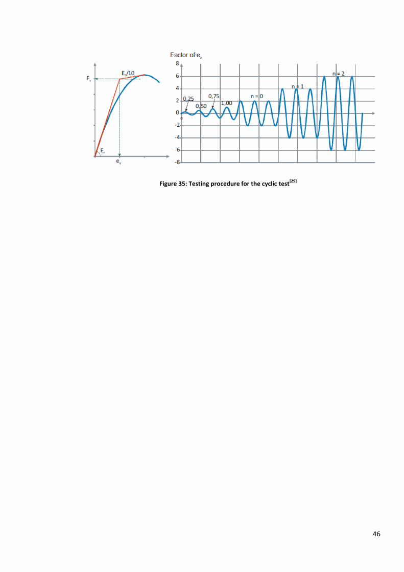
46

Figure 35: Testing procedure for the cyclic test[29]

47

5. Numerical testing in FineLg

In this chapter, the aspects of the numerical testing in this dissertation are explained. For all four

products considered in this dissertation, a 2D model in longitudinal direction was developed and

tested with the numerical package FineLg[13]. In the following text, the 2D model is explained in more

detail, followed by the different types of numerical tests that were performed on this model. For

each product, two kinds of models were developed with respect to the payload on the pallet beams,

namely a fully loaded and a top loaded model. In general, these two types are expected to be the

most critical for the design of storage racking systems.

5.1 2D model

For each of the four products, a 2D model with two bays and four levels was implemented in

FineLg[13]. The columns and beams were modelled as rectangular sections with the same area and

second moment of area as the real sections. The connectors and base plate connections were

modelled as rotation springs that were linearly constrained. In this way, only local rotation in the

connectors and base plate connections was possible. These springs were characterized by moment-

rotation curves. For this dissertation, use was made of the moment-rotation curves attained from the

tests conducted in Aachen[27] (See Chapter 4) and from design sheets given by the producers. In the

different tests stated below, a different use was made of these curves. In the figure below, an

example is given of a 2D model (Figure 36).

Figure 36: 2D model

As stated above, two different types of payload were used to do the analyses:

A fully loaded model: all eight beams were loaded;

A top loaded model: only the two top level beams were loaded;

48

The payload was modelled as concentrated masses in the modal analysis and as vertical forces in all

other analyses.

To model the seismic action on these systems, triangular distributed horizontal forces were used that

acted at each beam level of the model.

The beams and columns were modelled as linear elastic entities for all analyses done in this

dissertation. This means that only the stiffness was implemented in the models and no plastic zone

was assumed. This assumption is justified by the fact that storage racking systems are expected to

fail through excessive deformation of the beam-to-column connectors and column base connections

with the floor. So, by assuming the columns and beams as infinitely linear elastic, failure in all sorts of

analyses in this dissertation with FineLg[13] can only be achieved by plastic deformation of the

connectors and column bases. An extra beneficial fact of this assumption is that the behaviour of the

connectors and column bases can be analysed without disturbing effects from the deformation of

beams and columns.

5.2 Modal analysis

The first five modes of the 2D model, implemented in FineLg[13], could be attained by running a

modal analysis. In this analysis the payload on the pallets carried by the beams was modelled by

concentrated masses. Three masses were distributed on each beam in that way that the position of

each mass coincided with the centre of each pallet. Each mass had a weight of 400 kg, being half of

the total mass for each pallet used in design purposes, as the 2D model was in fact half of a real

storage rack in transverse direction. By attaining these modes, an estimation could be made for the

horizontal triangular distributed forces, used for running linear and nonlinear analyses in FineLg[13]. In

the figure below, a fully loaded model and a top loaded model is illustrated (Figure 37).

a) Fully loaded b) Top loaded Figure 37: Modal analysis

49

5.3 Monotonic analyses

For these analyses, the payload on the pallet beams was modelled by vertical forces, each exerting a

load of 1.308 kN. The expression below shows how this value was attained.

As each pallet stands for a payload of 400 kg and has three supports on a beam, three vertical forces

for each pallet were used. These were situated at the positions where the supports of the pallet on

the beam would be situated. In this analysis, the 2D model was pushed horizontally to one side by

triangular distributed forces. These forces were calculated out of the first mode attained from the

modal analysis. Under the next chapter, the calculating process for attaining these horizontal forces

is illustrated. In the figure below, a fully loaded model and a top loaded model is illustrated, showing

the vertical forces (The horizontal forces are too small to be seen accurate on the figures) (Figure 38).

a) Fully loaded b) Top loaded

Figure 38: 2D model with vertical and horizontal forces

50

5.3.1 Linear elastic analysis

Exerting a linear elastic analysis for the 2D model in FineLg[13] means that the connectors, base plates

columns and beams were modelled to be linear elastic and no limit or plastic zone was assumed. So

only the rotation spring stiffness for the connectors and base plates was needed from the data

attained by the test results of Aachen and the design sheets of the producers. Chapter four of this

dissertation is devoted to the tests conducted in Aachen. For this analysis, the constitutive law 0 was

used. This is Hooke's law, as illustrated in the figure below (Figure 39). Only the calculated triangular

distributed horizontal loads were implemented in the model for this analysis and no payload was

assumed.

Figure 39: Hooke's law (law 0)[30]

With this analysis, a load-displacement point was attained for the fully loaded and top loaded model.

This point was then extended to a line, connecting the point with the origin of the graph and using

the attained slope to extend the line for bigger loads. The main purpose of these curves was to

compare them with load-displacement curves achieved from the nonlinear analysis, where the

payload was implemented in the model. The goal of comparing these analyses was to prove that the

payload is responsible for the nonlinear behaviour a storage racking system exerts in a real-life

situation when exposed to seismic action.

5.3.2 Nonlinear analysis

For the nonlinear analysis, the payload was implemented in the model. Now, the beam-to-column

connectors and column base connections were modelled to be nonlinear. Three different subtypes of

analysis were performed in the nonlinear analysis. The difference is concentrated in the constitutive

material laws that were used to model the rotation springs for the beam-to-column connectors and

base plates. These three types of constitutive laws are treated in more detail in the subtitles below.

In the nonlinear analysis, use was made of sequence loading. The first sequence was the direct

appliance of the payload. Then the second sequence was applied, exerting the horizontal forces

incrementally through loading steps.

51

5.3.2.1 Nonlinear analysis using Hooke's law

For this analysis, the connectors and base connections were modelled with law 0 as was the case in

the linear elastic analysis. But because sequence loading was used, actual moment-displacement

curves were achieved and nonlinear behaviour was expected because of the payload. These curves

without plastic zone were generated to compare this kind of analysis with linear elastic analysis and

the other nonlinear analyses. Comparison of these curves with the curves attained from the linear

elastic analysis proved the nonlinear behaviour of storage racking systems as a result of the payload

on the pallet beams.

5.3.2.2 The elastic-perfectly plastic law

In FineLg[13], this law is implemented as law 1. For this constitutive law, the rotation spring stiffness

and a yielding point were implemented to run the analysis. The shape of this law is illustrated in the

figure below (Figure 40). Numerical values for the yielding points were adopted from the test results

conducted in Aachen[27] and the design sheets of the producers (See Chapter 6). The design curves of

the products were used, as these design curves also show an elastic-perfectly plastic course. From

this type of analysis, pushover curves were generated. As there was a plastic zone implemented in

the model for the connectors and base connections, these curves were expected to show a maximum

value of load. By performing this analysis, the nonlinear behaviour of the storage racking system

could be evaluated. Furthermore, comparison of the attained load-displacement curves with the

curves attained using piecewise linear constitutive laws (see next subtitle) for the connectors

resulted in an evaluation of whether the design of storage racking systems according to the design

curves is either safe or not.

Figure 40: Elastic - perfectly plastic law (law 1)[30]

52

5.3.2.3 The piecewise linear law

With this constitutive law, implemented as law 11 in FineLg[13], a better approximation of the

moment-rotation curves for the connectors was made. As no moment-rotation curves for the column

base connections were available, the elastic-perfectly plastic law (law 1) was used for these rotation

springs. The moment-rotation curves resulted out of the tests conducted in Aachen[27] (See Chapters

4 and 6). Coordinates were derived out of these moment-rotation curves and were implemented in

the model. The piecewise linear law connects these coordinates by straight lines giving a realistic

approximation of the moment-rotation curve. The only deficiency of this law is the fact that only a

rising course can be drawn. So, the descending part of the moment-rotation curves, where the

moment is diminishing in value, could not be modelled. An illustration of this stepwise linear law is

shown in the figure below (Figure 41). To use this law, also an initial stiffness and a final stiffness

value are to be implemented. For the initial stiffness, the values were adopted from Table 2 (Chapter

4) that summarizes initial stiffness values for the beam-to-column connections. For the final stiffness,

the value zero was used. This means that the last straight line in the figure below is a horizontal line.

Also for this analysis, pushover curves were generated. These load-displacement curves were

assumed to be more realistic than those resulting from the analyses using elastic-perfectly plastic

laws.

Figure 41: Piecewise linear law (law 11)[30]

At the end of the monotonic analyses for each product, all curves attained from the different types of

monotonic analyses illustrated above were plotted together in one graph. By doing this, conclusions

about the behaviour of the models could be drawn more easily.

53

5.4 Cyclic and dynamic analyses

In reality, the behaviour of a storage racking system subjected to seismic action is also evaluated

through cyclic and dynamic tests. As this dissertation was mainly concentrated on monotonic

numerical testing, cyclic and dynamic analyses were only performed illustratively for product B, for

the fully loaded case (as the top loaded case was less critical than the fully loaded case (see chapter

7)). First, the cyclic analysis is shortly explained, followed by the dynamic analysis.

5.4.1 Cyclic analyses

In the cyclic analysis, the structure was pushed back and forth to growing values of displacement. So,

in this case, the horizontal forces on the structure were replaced by displacements. The limits were

determined out of the monotonic pushover curves from the nonlinear analyses with plastic zone. To

be able to impose displacements on the structure, four extra supports had to be implemented in the

model in FineLg[13] at each beam level. These supports only restrained horizontal displacement (See

Figure 42). The results of these analyses were also translated to load-displacement curves. Here, the

horizontal reactions of the extra supports are achieved instead of load multipliers. In this way, a

comparison could be made with the monotonic pushover curves. To do so, the total base shear force

was calculated and put on the vertical axis of the graph. The horizontal axis showed the

displacements of the top node during the analysis.

Figure 42: Extra supports

In this dissertation, a cyclic analysis was done for material law 1 and 11 and the curves were then put

together with the monotonic pushover curves in one graph for each material law.

54

5.4.2 Dynamic analyses

With a dynamic analysis, a situation could be simulated that is very close to a real seismic event. In

FineLg[13], the horizontal loading of the structure was now achieved through implementation of a set

of ground accelerations that applied at the column bases. According to Eurocode 8[3], this set of

ground accelerations is to be determined so that they exhibit the same response spectrum as the

one chosen for the design of the storage racks. In this case, a type 1 response spectrum on soil type C

applied. Furthermore, the code states that seven sets of ground accelerations are to be used in order

to achieve an accurate analysis. Only the mean result from these seven simulations is to be used for

proper evaluation.

In this dissertation, one linear and two nonlinear dynamic analyses with material law 1 and 11 were

performed for one set of ground accelerations. In this way, an idea could be given about the

behaviour of the storage rack during such a test. Therefore, time-displacement curves were

generated.

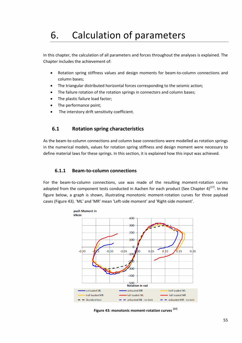
55

6. Calculation of parameters

In this chapter, the calculation of all parameters and forces throughout the analyses is explained. The

Chapter includes the achievement of:

Rotation spring stiffness values and design moments for beam-to-column connections and

column bases;

The triangular distributed horizontal forces corresponding to the seismic action;

The failure rotation of the rotation springs in connectors and column bases;

The plastic failure load factor;

The performance point;

The interstory drift sensitivity coefficient.

6.1 Rotation spring characteristics

As the beam-to-column connections and column base connections were modelled as rotation springs

in the numerical models, values for rotation spring stiffness and design moment were necessary to

define material laws for these springs. In this section, it is explained how this input was achieved.

6.1.1 Beam-to-column connections

For the beam-to-column connections, use was made of the resulting moment-rotation curves

adopted from the component tests conducted in Aachen for each product (See Chapter 4)[27]. In the

figure below, a graph is shown, illustrating monotonic moment-rotation curves for three payload

cases (Figure 43). 'ML' and 'MR' mean 'Left-side moment' and 'Right-side moment'.

Figure 43: monotonic moment-rotation curves [27]

56

Depending on the type of analysis done, the following values were to be derived from curves like

those in the figure:

Modal analysis, linear elastic analysis and nonlinear elastic analysis (law 0): initial stiffness;

nonlinear analysis (law 1): initial stiffness and design moment (= maximum value);

nonlinear analysis (law 11): coordinates of the moment-rotation curve.

To perform accurate dynamic analyses, cyclic moment-rotation curves are to be used similarly to

achieve the right values. An example of such curves for one payload case is given in the graph below

(Figure 44). In this dissertation, no use was made of these curves for the dynamic analyses

performed, as the illustrative tests used material laws 1 and 11.

Figure 44: Cyclic moment-rotation curves[27]

For the analyses done in this dissertation, only the fully loaded case and the unloaded case needed to

be considered for the beam-to-column connectors, as the two models used were a top loaded model

and a fully loaded model.

6.1.2 Column base connections

Initially, the intention was to achieve values for rotation stiffness and design moment in a similar way

as for the beam-to-column connections. But, as the component tests for column bases in Aachen

experienced significant delay, no moment-rotation curves were available at the time of writing (See

also Chapters 3 and 4). As a result of this, the decision was made to use available information from

the producers. Typically, the information received are tables with different values for stiffness and

maximum moment, for different values of axial load applied to the columns.

For the fully loaded and top loaded model used in this dissertation, four different values of axial load

were met:

57

Fully loaded model;

o Exterior column base: F =23.544 kN;

o Interior column base: F = 47.088 kN.

Top loaded model.

o Exterior column base: F = 5.886 kN;

o Interior column base: F = 11.772 kN.

Frequently, these values did not match with the values in the tables received from the producers. To

solve this problem, the values from the received tables were plotted in 'stiffness-axial load graphs'

and 'design moment-axial load graphs' for each product. Then, interpolation was utilized to achieve

accurate values in function of the respective axial loads stated above. An illustration of the

interpolation for rotation stiffness for one product is given in the figure below (Figure 45).

Figure 45: Interpolation for column base rotation stiffness

Only initial rotation stiffness and design moment values could be derived from these graphs.

Consequently, no material law 11 could be implemented for the column bases in the numerical

models. For the modal and elastic analyses (law 0), the initial stiffness was implemented. For all

nonlinear analyses, only law 1 could be used, meaning an implementation of initial stiffness and

design moment. This was the case for monotonic, cyclic and dynamic analyses.

58

6.2 Triangular distributed horizontal forces - seismic action

To do linear and nonlinear numerical testing and thus to generate pushover curves, the seismic

action on the structure was converted to a set of horizontal forces that were triangularly distributed

in the vertical direction. These forces replaced a total base shear force at the bottom of the structure

that would be exerted by an earthquake on a storage rack. To calculate these horizontal forces, the

following process was used. This process is recommended by Eurocode 8[3] and is also illustrated in

the course 'Seismic Design' by Prof. Hervé Degée[31].

6.2.1 Modal analysis

First, a modal analysis was run in FineLg to calculate the first five modes of the 2D model. If the first

mode has a percentage of collaborate mass of at least 90%, then only this first mode has to be used

in the calculating process. Otherwise, more modes have to be considered in the calculation.

In the modal analyses for the four products, the first mode always had a percentage of collaborate

mass of more than 85%, but less than 90%. As this percentage was close to 90%, it was assumed that

only the first mode was to be used in the calculating process.

So for each model, the first mode was maintained from the modal analysis and the first period T1 was

calculated.

6.2.2 Calculation of the base shear force

The base shear force was calculated according to the following equation:

with:

: the ordinate of the design spectrum at period T1 (m/s²);

: the correction factor (-);

Mtot: the total mass of the structure above the foundation (kg).

In what follows, the calculation of these three parameters is illustrated.

59

6.2.2.1 The ordinate of the design spectrum

For the calculation of , Eurocode 8 recommends the following expressions:

:

:

:

:

with:

: the design ground acceleration;

S: the soil factor;

, and : the limits that define the response spectrum (see figure 46);

q: the behaviour factor;

: the lower bound factor for the horizontal design spectrum.

Figure 46: Shape of the response spectrum

[3]

For all four products, a soil type and a spectrum type had to be chosen to get the values of S, ,

and . In this case, a soil type C and a spectrum type II was preconceived for products A, C and D.

For product B, a soil type C and a spectrum type I was chosen. The characteristics of these spectra

are summarized in the table below (Table 3).

60

Table 3: Characteristics of the seismic response spectrum[3]

Product S TB (s) TC (s) TD (s)

A,C &D 1.5 0.10 0.25 1.20

B 1.15 0.20 0.60 2.00

Furthermore, a value for the design ground acceleration, the behaviour factor and the lower bound

factor had to be chosen. For , the recommended value is equal to 0.2 and was used here.

By comparing the value of T1 and the other T-values, the right equation was chosen and the value of

could be computed.

6.2.2.2 The correction factor λ

According to EC8[3], there are two possible values for the correction factor:

if and the structure has more than two storeys;

otherwise.

For all four products, it was seen that the value of was always bigger than two times the value of

, resulting in a value for lambda equal to unity.

6.2.2.3 The total mass of the structure

For the calculation of the total mass, Eurocode 8 states the following expression[3]:

with:

: the combination coefficient for variable action;

g: the gravity acceleration ( 9.81 m/s²) .

The combination coefficient was calculated as follows:

According to Eurocode 0[32], storage racking systems are included in Category E. As a result of this,

the values of and the combination factor are 1.0 and 0.8 respectively. So, the value for for

all four storage racks was:

61

The payload was assumed to be a live load and the columns and beams that form the storage rack

were assumed to be dead load. As the weight of the dead load was much smaller than the payload (<

5% of the sum of dead and live loads), the dead load was neglected in the calculation of the total

mass. So, for each product the total mass had the same value and was calculated as follows:

Fully loaded 2D model:

Top loaded 2D model:

6.2.3 Calculation of the triangular distributed horizontal forces

To compute these horizontal forces out of the base shear force, the following expression is given in

EC8[3]:

Where zi and zj are the heights of the masses mi and mj respectively above the level of application of

the seismic action.

For the fully loaded case, the distribution of the masses was the same for each storey. So the

expression above could be simplified as follows:

For the top loaded case, all the mass was distributed at the top level. So, all the force was

concentrated at the top level, giving:

These horizontal forces were vertically positioned at the centre of each beam as shown in the figure

below (Figure 47). With these forces, all numerical monotonic linear and nonlinear tests were

performed in FineLg.

62

Figure 47: Triangular distribution of seismic horizontal forces

6.3 Failure rotation for connections

The failure rotations of beam-to-column and column base rotation springs were necessary to cut off

the pushover curves generated in FineLg[13]. These curves were typically generated for 42 loading

steps, ignoring a maximum rotation by which in reality the beam-to-column connectors or column

bases would break. In order to account for this phenomenon, the failure rotations were estimated

and the curves were cut off at the loading step where the first failure rotation was met either for the

connectors or the column bases. The estimation of these failure rotations was done as follows.

Moment-rotation curves for the beam-to-column connectors and the column base connections were

used to attain the maximum moment Mmax. The diagrams for the connectors were extracted from

the tests performed in Aachen[27]. The diagrams for the column base connections were drawn from

the report of the SEISRACKS project[1].

In practice, it is common to assume that the failure rotation Фu is situated at the point on the curve,

passed the maximum moment, where the moment is equal to:

This is illustrated in the figure below (Figure 48).

63

Figure 48: Practical method for attaining the failure rotation Фu

As was proven by the results of the tests performed in Aachen on the connectors[27], moment-

rotation curves are influenced by the payload on the beams. So for the beam-to-column connectors,

difference was made between fully loaded and unloaded pallet beams. For the fully loaded model,

only the fully loaded condition had to be used. For the top loaded model, both the fully loaded and

the unloaded condition had to be taken into consideration.

For column bases, the moment-rotation curves are influenced by the axial load that is present in the

column. As a result of this, difference existed between the interior column base and the exterior

column bases and also between the fully loaded model and the top loaded model. At the time of

performing the analyses, the tests on column bases in down-aisle direction were not yet performed

in the SEISRACKS 2-project and use was made of the curves available in the report of SEISRACKS[1].

These curves are illustrated in the figure below (Figure 49). The curves available were generated with

axial loads of 1, 25, 50 and 75 kN. For other values of the axial load, an interpolation between the

curves was made to achieve an approaching value for the maximum rotation.

Figure 49: Moment-rotation curves for column bases on concrete deck[1]

64

In the table below, an overview of the required maximum rotations is given for the connectors and

column bases, for both the fully loaded and top loaded model (Table 4).

Table 4: Overview of required maximum rotations

Model Connector Interior column base Exterior column base

Loading case Axial load (kN) Axial load (kN)

Fully loaded Fully loaded 47.088 23.544

Top loaded Fully loaded 11.772 5.886

Unloaded

6.4 Plastic failure load factor

The plastic failure load factor λP is a measure for the plastic capacity a structure possesses. As a

matter of fact, it is the factor by which the applied load has to be multiplied to transfer the structure

into a complete mechanism.

The plastic failure load factor was calculated assuming that all connectors and column bases had

yielded and the 2D model was swayed sideways. The computation was done as follows and was

adopted from the course 'Nonlinear and plastic methods of structural analysis'[33]. This calculation

method is a first order calculation, meaning that second order effects are not incorporated in the

calculation.

6.4.1 Fully loaded model

For the fully loaded model, the calculation is illustrated in the figure below (Figure 50).

65

Figure 50: Calculation model for fully loaded case

As the beams were assumed to stay horizontal in the mechanism, the vertical forces representing the

payload did not perform any work and hence could be neglected in the calculation. Only the

horizontal forces were performing work during the displacement of the mechanism. The failure load

factor was calculated through the following steps.

with:

: the horizontal seismic force at height ;

: the horizontal displacement at height ;

: the plastic moment of entity i (i.e. a connector or a column base);

: the relative rotation of the connected elements with respect to the initial condition;

: the plastic moment of the connectors attached to fully loaded beams;

: the plastic moment of the exterior column bases;

: the plastic moment of the interior column base.

66

6.4.2 Top loaded model

The figure below shows the calculation model for the top loaded case (Figure 51).

Figure 51: Calculation model for top loaded case

Again, only the horizontal force was taken into account for the calculation of the failure load factor.

Analogous to the calculation for the fully loaded case, the failure load factor was computed as

follows:

with:

: the plastic moment of the connectors attached to unloaded beams.

The calculation for the fully loaded model and the top loaded model was done for the nonlinear

analysis with constitutive law '1' and with the piecewise constitutive law '11', as the plastic moment

values for the beam-to-column connectors were different for both laws.

By putting this plastic failure load factor on the pushover curves, the difference between the

maximum of the pushover curve and this load factor could be evaluated. This is illustrated in the

67

figure below (Figure 52). This difference is a measure for the limitation of the plastic reserve of the

structure and especially the influence of second order effects on the structure.

Figure 52: on pushover curve

6.5 Performance point

The performance point or target displacement is defined as the seismic demand, in terms of

displacement, a structure has to provide to persist a given applied seismic action.

Calculating the performance point and putting it on the load-displacement curve for each model gave

an idea of whether the existent storage rack was designed optimally or not. If this point was situated

on the linear elastic part of the curve, then the structure was conservatively designed for the seismic

action. On the other hand, if this point was situated too far in the plastic zone, the structure could fail

before reaching the required deformation. For an optimally designed structure, the position of the

performance point should be somewhere between the curve maximum and the failure displacement

of the structure. In this zone, the structure is already deforming plastically, but no components have

failed yet.

The calculation of this performance point is illustrated in EN 1998-1 Annex B: 'Determination of the

target displacement for nonlinear static (pushover) analysis[3]. In what follows, the calculation

process stated in the code is explained.

The target displacement is determined from the elastic response spectrum. Also, the capacity curve

is needed. This curve represents the relation between base shear force and control node

displacement.

68

6.5.1 Normalisation

First, the displacements are normalized in such a way that Фn = 1 where n is the control node. With

this normalization, the following relation between normalized lateral forces and normalized

displacements is assumed:

where is the mass in the i-th storey.

For the models used in this dissertation, the first modal shape was assumed to be triangularly

distributed in the vertical direction. So, the values for the normalized displacements were:

(≈first beam level)

(≈second beam level)

(≈third beam level)

(≈column top)

The mass for each storey was equal to 0.8 (=ΨE) times 2400 kg for fully loaded storeys or 0 kg in case

of unloaded storeys. So, the following normalized forces applied:

Fully loaded model:

Top loaded model:

69

6.5.2 Transformation to an equivalent Single Degree of Freedom system

The models used in this dissertation are Multi Degree of Freedom systems (MDOF). To calculate the

target displacement, a transformation is needed to an equivalent Single Degree of Freedom system

(SDOF). To do so, the following parameters are calculated:

The mass of the SDOF system:

The transformation factor:

The force of the SDOF system:

with equal to the base shear force of the MDOF system.

The displacement of the SDOF system:

with equal to the control node displacement of the MDOF system.

For all the models used in this dissertation, the following values were calculated for the mass of the

SDOF system and the transformation factor:

Fully loaded model:

Top loaded model:

70

As for the top loaded model only the top level beam was loaded, the top loaded model acted as a

SDOF system directly. For the calculation of the force and displacement of the SDOF system, each

product exhibited different values for the base shear force and the control node displacement.

6.5.3 Idealized elastic-perfectly plastic force-displacement relationship

Now, an idealized elastic-perfectly plastic law is defined in such a way as illustrated by the figure

below (Figure 53). The yield force represents the ultimate strength of the idealized system and is

equal to the base shear force at the formation of the plastic mechanism. The slope of the elastic part

of the idealized system is determined in such a way that the areas under the idealized curve and the

actual force-displacement curve are equal to each other. Taking into account this assumption, the

yield displacement of the idealized system is calculated by following expression:

with the actual deformation energy up to the formation of the plastic mechanism A.

For the models in this dissertation, the attained pushover curves were different for each product. As

a result of this, each model showed other values for the parameters in this section and for the

remainder of the calculation process.

Figure 53: Definition of elastic-perfectly plastic force-displacement curve[3]

71

6.5.4 Period of the idealized equivalent SDOF system

As the target displacement is calculated according to the elastic response spectrum, a period is

needed to determine the right expression for the calculation of the ordinate of this response

spectrum .

The period is calculated as follows:

6.5.5 Target displacement for the equivalent SDOF system

The target displacement is first calculated assuming unlimited elastic behaviour:

with the elastic acceleration response spectrum evaluated at , determined with one of the

following expressions:

:

:

:

:

All coefficients are the same as those defined in the second section of this chapter. For the damping

correction factor , the recommended value is equal to 1.0, corresponding to 5% viscous damping.

The target displacement is then calculated by the following expressions, making difference

between structures in the short-period range and the medium to long-period range. The corner

period for this difference is .

6.5.5.1 Short period range ( < )

In this case, the response can be either elastic or nonlinear.

The response is elastic if:

72

and the target displacement is:

The response is nonlinear if:

and the target displacement is calculated as follows:

with:

The figure below illustrates the calculation process for the short period range (Figure 54).

Figure 54: Target displacement for the short period range

[3]

6.5.5.2 Medium to Long period range ( )

The target displacement is calculated as follows:

The figure below illustrates the process for the medium to long period range (Figure 55).

73

Figure 55: Target displacement for the medium to long period range

[3]

If the target displacement is much different from the displacement

used for the determination

of the idealized elastic-perfectly plastic force-displacement relationship (see 6.4.3), an iterative

procedure may be applied, in which the process through subtitles 6.4.3 - 6.4.5 is repeated by

replacing by

in the expression stated in 6.4.3 and using the corresponding value for .

6.5.6 Target displacement for the MDOF system

Finally, the target displacement is transformed back to the MDOF value:

This target displacement corresponds to the control node.

6.6 Interstorey drift sensitivity coefficient

Storage racking systems commonly are sensitive to P-Delta effects, also called second-order effects.

To answer the question whether these P-Delta effects are to be accounted for in the structural

analysis, Eurocode 8[3] and FEM 10.2.08[2] recommend to calculate the so-called -parameter. This

parameter is defined according to the following equation and Figure 56 (See also section 2.4.4.2).

with:

: the total gravity load at and above the considered storey

: the design interstorey drift evaluated as the difference of the average lateral

displacement at the top and bottom of the considered storey;

: the total seismic storey shear;

: the interstorey height.

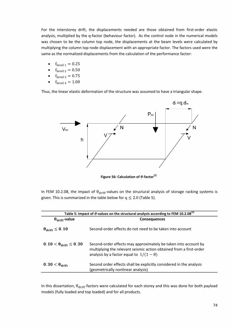
74

For the interstorey drift, the displacements needed are those obtained from first-order elastic

analysis, multiplied by the q-factor (behaviour factor). As the control node in the numerical models

was chosen to be the column top node, the displacements at the beam levels were calculated by

multiplying the column top node displacement with an appropriate factor. The factors used were the

same as the normalized displacements from the calculation of the performance factor:

Thus, the linear elastic deformation of the structure was assumed to have a triangular shape.

Figure 56: Calculation of -factor[2]

In FEM 10.2.08, the impact of -values on the structural analysis of storage racking systems is

given. This is summarized in the table below for (Table 5).

Table 5: Impact of -values on the structural analysis according to FEM 10.2.08[2]

-value Consequences

Second-order effects do not need to be taken into account

Second-order effects may approximately be taken into account by multiplying the relevant seismic action obtained from a first-order analysis by a factor equal to

Second order effects shall be explicitly considered in the analysis (geometrically nonlinear analysis)

In this dissertation, -factors were calculated for each storey and this was done for both payload

models (fully loaded and top loaded) and for all products.

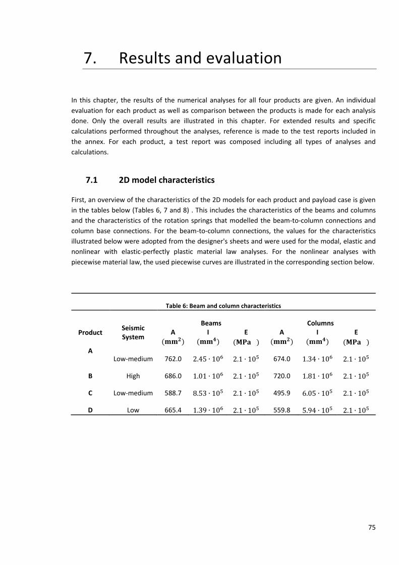
75

7. Results and evaluation

In this chapter, the results of the numerical analyses for all four products are given. An individual

evaluation for each product as well as comparison between the products is made for each analysis

done. Only the overall results are illustrated in this chapter. For extended results and specific

calculations performed throughout the analyses, reference is made to the test reports included in

the annex. For each product, a test report was composed including all types of analyses and

calculations.

7.1 2D model characteristics

First, an overview of the characteristics of the 2D models for each product and payload case is given

in the tables below (Tables 6, 7 and 8) . This includes the characteristics of the beams and columns

and the characteristics of the rotation springs that modelled the beam-to-column connections and

column base connections. For the beam-to-column connections, the values for the characteristics

illustrated below were adopted from the designer's sheets and were used for the modal, elastic and

nonlinear with elastic-perfectly plastic material law analyses. For the nonlinear analyses with

piecewise material law, the used piecewise curves are illustrated in the corresponding section below.

Table 6: Beam and column characteristics

Product Seismic System

Beams Columns A

I

E

A

I

E

A

Low-medium 762.0 674.0

B High 686.0 720.0

C Low-medium 588.7 495.9

D Low 665.4 559.8

76

Table 7: Rotation spring characteristics (designer's sheets)

Product Seismic System

Beam-to-column rotation springs

A Low-medium 139.450 1.437

B High 170.601 3.405

C Low-medium 112.448 2.589

D Low 112.448 2.589

Table 8: Rotation spring characteristics (designer's sheets)

Product Seismic System Loading case - position Column base rotation springs

A Low-medium Fully loaded - interior 535.584 1.179

Fully loaded - exterior 237.022 0.962

Top loaded - interior 75.268 0.815

Top loaded - exterior 37.634 0.733

B High Fully loaded - interior 297.558 2.433

Fully loaded - exterior 135.326 1.349

Top loaded - interior 67.663 0.811

Top loaded - exterior 33.832 0.542

C Low-medium Fully loaded - interior 198.554 1.739

Fully loaded - exterior 145.579 1.054

Top loaded - interior 79.756 0.548

Top loaded - exterior 39.880 0.2744

D Low Fully loaded - interior 156.715 1.795

Fully loaded - exterior 83.023 0.993

Top loaded - interior 41.240 0.591

Top loaded - exterior 20.620 0.392

77

7.2 Modal analysis

For the fully loaded and top loaded model, a modal analysis had to be performed to achieve the

necessary triangular distributed horizontal forces. These horizontal forces were used to perform the

other analyses. In the tables below, the first mode for all four products is given for the fully loaded

and top loaded case (Tables 9 and 10). Only the first mode was used in the horizontal forces

calculation process.

7.2.1 Fully loaded case

Table 9: First mode (fully loaded case)

Product Frequence (Hz) Period (s) Percentage of collaborate mass (%)

A 0.447 2.235 84.169

B 0.435 2.297 85.351

C 0.349 2.864 85.015

D 0.348 2.873 86.636

For all products, the first periods lie pretty much close to each other. The values are quite high as one

sees that these values are bigger than the TD-values from the elastic response spectrum used (see

Eurocode 8[3]). The lowest value is observed for product A. This is logical when one looks at the

stiffness values in the tables above (Section 7.1). The column base stiffness values are significantly

higher for product A and the beam-to-column connection stiffness values are the second largest of all

products. Consequently, product A is most stiff and its period is the lowest.

product B has the second lowest period because this product possesses the most stiff beam-to-

column connections. As the column base stiffness is significantly lower than for product A, its first

period is a bit higher than for the latter product.

products C and D have beam-to-column connection and column base stiffness that are very similar.

As the column base stiffness for product D are a bit smaller than for product C, its first period is

slightly bigger.

The percentage of collaborate mass gives percentages around 85 %. As stated in Chapter 6, this

percentage should be 90% or higher to calculate the seismic action on the structure. Here it was

assumed that this percentage was sufficient to calculate accurate seismic action and thus also the

triangular distributed horizontal forces.

78

7.2.2 Top loaded case

Table 10: First mode (top loaded case)

Product Frequence (Hz) Period (s) Percentage of collaborate mass (%)

A 0.556 1.799 100

B 0.559 1.789 100

C 0.460 2.172 100

D 0.459 2.176 100

Similarly as for the fully loaded case, the periods lie close to each other. For product B, this period is

lower than the used TD-value of the elastic response spectrum (TD = 2.0 s). For the other products,

the first period is bigger than TD (TD = 1.2 s).

For the top loaded case, one sees that the lowest period is found for product B. This means that the

column base connections under lower axial loads are more stiff than the column bases of the other

products under the same loading conditions. For products C and D, the same conclusions can be

drawn as for the fully loaded case.

As there is only one period for this payload case, it is logical that the percentage of collaborate mass

is equal to 100%. So, no assumptions were to be made here for the calculation of the seismic action.

7.2.3 Comparison between the payload cases

For each product, the first period is lower for the top loaded case than for the fully loaded case. This

is logical because, despite the lower stiffness values for the column base connections, less mass is

present in the top loaded case, resulting in less total inertial force. This inertial force counteracts the

movement of the structure. The bigger this force is, the slower the rack will vibrate and the bigger its

first period. The decrease in payload has a bigger influence on the first mode than the decline in

stiffness of the column bases.

79

7.3 Seismic action

In this section, the triangular distributed horizontal forces are given for each product, for both

payload cases. For product A, C and D these forces were calculated using a type 2 response spectrum

and soil class C. For product B, use was made of the type 1 response spectrum for the same soil class.

The detailed calculation can be found in the test reports in the annex. Tables 11 and 12 provide the

seismic action for all products for the fully loaded and top loaded case, respectively.

7.3.1 Fully loaded case

For the fully loaded case, the base shear force was subdivided in four horizontal forces. Each force

was applied at a beam level. In the table below, the forces are numbered from bottom to top beam

level.

Table 11: Seismic action (fully loaded case)

Product F1 (kN) F2 (kN) F3 (kN) F4 (kN)

A 0.152 0.304 0.456 0.608

B 0.509 1.032 1.555 2.078

C 0.222 0.451 0.679 0.908

D 0.181 0.367 0.554 0.741

When looking at the forces, product B has significant higher forces. This is the result of using the type

1 response spectrum instead of type 2. For the other products, the differences are not that big, cause

for all these products, the response spectrum type 2 was used. The lowest values observed are those

for product A.

7.3.2 Top loaded case

For the top loaded case, the base shear force was completely transmitted to the fourth level, as this

level was the only one that carried payload. In the table below, these forces are given (Table 12).

80

Table 12: Seismic action (top loaded case)

Product F4 (kN)

A 0.380

B 1.907

C 0.565

D 0.461

Also for the top loaded case, a huge difference is seen for the force of product B. Again, the reason is

the choice of a type 1 spectrum instead of type 2. The values for the other products lie again close to

each other. Also in the top loaded case, the lowest force is the one for product A.

7.3.3 Comparison between the payload cases

When comparing the payload cases for each product, it is mentioned that the top loaded case base

shear force lies between F2 and F3 of the fully loaded case for products A, C and D. For product B, this

force lies between F3 and F4 of the fully loaded case.

7.4 Monotonic analyses

The forces calculated above were used to generate load-displacement curves for different types of

analyses. Four monotonic analyses were performed for each product and payload case:

Linear elastic analysis (law 0);

Nonlinear elastic analysis (law 0);

Nonlinear analysis (law 1);

Nonlinear analysis (law 11).

For detailed information about these analyses, reference is made to Chapter 5 and the test reports in

the annex.

The results of these analyses were translated to load-displacement curves. The curves presented

here are in fact 'load multiplier-displacement curves'. The load multiplier is the factor by which the

calculated horizontal forces above were multiplied during the numerical tests. These curves are also

called 'pushover curves' as the structure is pushed in one direction during the tests.

81

7.4.1 Linear and nonlinear elastic analysis

These type of analyses were carried out assuming elastic behaviour of the storage racking system.

The material laws for the rotation springs were all set to 'law 0'. In this section, a comparison is made

between the load-displacement curves of both analyses for each product and a comparison is made

between the four products. First, the fully loaded case (Figure 57) is treated followed by the top

loaded case (Figure 58). Second, a global comparison is made between fully loaded and top loaded

cases. It has to be mentioned that the curves presented in this section reach extreme displacements.

These displacements would not be met in reality because the connections between the racks would

have failed already before these displacements are met. However, by presenting the curves below

like this, some illustrative observations are displayed more clear. In the section 'Calculated

parameters' the determined failure rotations for the connections are summarized and in the section

'Synthesis', all curves, cut off according to the failure rotations, are presented together.

7.4.1.1 Fully loaded case

On the curves below, the effect of the payload on the nonlinear behaviour is clearly seen for all

products. The 'FL Linear' curve is a straight line, while the other curve has an initial straight part

followed by a curved part. Moreover, this latter curve exerts a smaller slope.

Qualitatively, the degree of nonlinearity for each product can be determined by calculating the

fraction between both load multipliers for a certain displacement. The determination of these

fractions for a fixed realistic displacement of 0.30 m resulted in the following values (Table 13):

Table 13: Calculated fractions (fully loaded case)

Product Fraction (%)

A 78.85

B 77.60

C 64.50

D 63.68

From the table above, it is concluded that products C and D behave more nonlinear than the other

two products. This result was expected, as products A and B have bigger values for the rotation

spring stiffness. The bigger the stiffness of the system, the more the 'FL Nonlinear' curve will

approach the 'FL Linear' curve. Product D shows the most nonlinearity, product A the least.

82

Product A

Product B

0

10

20

30

40

50

60

70

80

90

0,00 0,50 1,00 1,50 2,00 2,50 3,00

Load

mu

ltip

lier

Displacement (m)

Elastic analysis

FL Linear

FL Nonlinear

0

5

10

15

20

25

30

0,00 0,50 1,00 1,50 2,00 2,50 3,00 3,50

Load

mu

ltip

lier

Displacement (m)

Elastic analysis

FL Nonlinear

FL Linear

83

Product C

Product D

Figure 57: Elastic analysis curves (fully loaded case)

0

5

10

15

20

25

30

35

40

45

0,00 0,50 1,00 1,50 2,00 2,50 3,00 3,50

Load

mu

ltip

lier

Displacement (m)

Elastic analysis

FL Nonlinear

FL Linear

0

10

20

30

40

50

60

0,00 0,50 1,00 1,50 2,00 2,50 3,00 3,50

Load

mu

ltip

lier

Displacement (m)

Elastic analysis

FL Linear

FL Nonlinear

84

7.4.1.2 Top loaded case

For the top loaded case, it can be observed that both curves approach each other more than for the

fully loaded case, proving that the nonlinear behaviour of storage racking systems is influenced by

the payload. In the same way as for the fully loaded case, the fractions are calculated for all four

products. These are illustrated in the table below (Table 14).

Table 14: Calculated fractions (top loaded case)

Product Fraction (%)

A 89.63

B 89.82

C 84.44

D 84.57

As expected, the values in the table above are bigger than those for the fully loaded case, proving

that the nonlinear behaviour is smaller when the payload is smaller. For this payload case, product C

shows the most nonlinearity and product B the least.

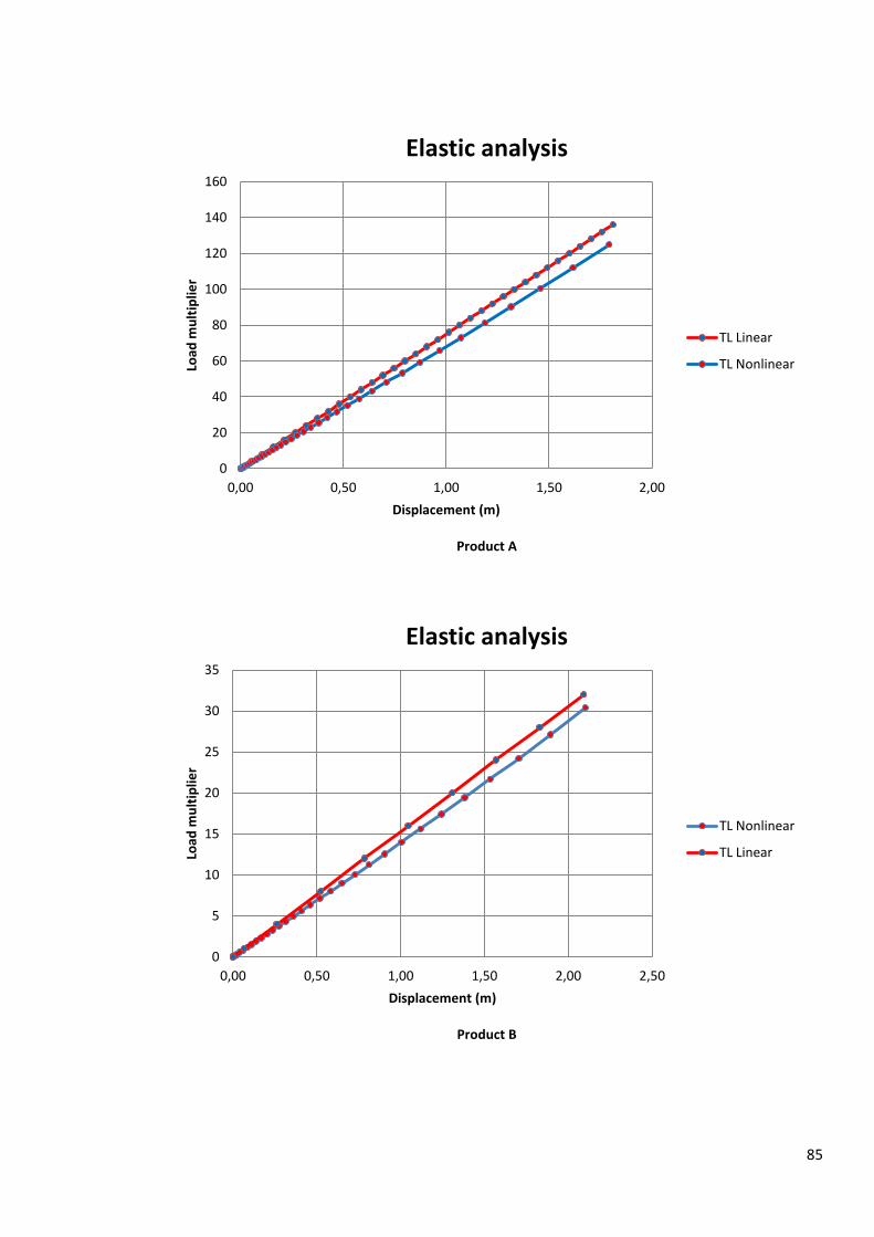
85

Product A

Product B

0

20

40

60

80

100

120

140

160

0,00 0,50 1,00 1,50 2,00

Load

mu

ltip

lier

Displacement (m)

Elastic analysis

TL Linear

TL Nonlinear

0

5

10

15

20

25

30

35

0,00 0,50 1,00 1,50 2,00 2,50

Load

mu

ltip

lier

Displacement (m)

Elastic analysis

TL Nonlinear

TL Linear

86

Product C

Product D

Figure 58: Elastic analysis curves (top loaded case)

0

10

20

30

40

50

60

70

80

0,00 0,50 1,00 1,50 2,00 2,50

Load

mu

ltip

lier

Displacement (m)

Elastic analysis

TL Nonlinear

TL Linear

0

10

20

30

40

50

60

70

80

90

100

0,00 0,50 1,00 1,50 2,00 2,50

Load

mu

ltip

lier

Displacement (m)

Elastic analysis

TL Linear

TL Nonlinear

87

7.4.1.3 Comparison between the payload cases

When comparing both payload cases, it is observed that the qualitative fraction values for

nonlinearity are higher for the top loaded case than for the fully loaded case. This result proves that

the degree of nonlinearity is smaller when the payload on the storage racking system is smaller.

Moreover, it is seen that the difference between the fractions is smaller for products A and B than

for the other two products. As products A and B have a larger overall stiffness, this means that the

influence of the payload on the nonlinearity is smaller when the stiffness is larger.

Furthermore it is noticed that for the fully loaded case, the difference between the fractions for

products A and B and products C and D is larger than the same difference for the top loaded case.

This means that the influence of the overall stiffness of the structure on the nonlinearity is bigger

when the payload is bigger.

7.4.2 Nonlinear analyses with plastic zone

For these types of analysis, a plastic zone was implemented in the numerical model. This was done in

two ways, using different constitutive material laws for the beam-to-column connectors. These were

'law 1' and 'law 11'. First, the piecewise material law curves for the 'law 11'-analysis are illustrated

for each product (Figure 59). Second, for each product and payload case, one graph is shown below

presenting both analyses together (Figure 60 and 61). In the text below, a comparison between both

curves for each product and payload case is performed. Furthermore, global comparison between

the products and the payload cases is provided.

Notice that the load-displacement curves below are cut off when the load multiplier reaches

negative values. For all the models, failure of the column bases and a lot of beam-to-column

connections was achieved before the end of the curves was reached. In this section, the descending

part of the curves is shown for indicative reasons. In the 'Synthesis' section, where all analyses are

put together in one graph, the curves will be cut off according to the calculated failure rotations (see

Chapter 6).

7.4.2.1 Piecewise material laws

For each product, one graph is given with the material laws for the beam-to-column connections for

a fully loaded and an unloaded pallet beam.

88

Product A

Product B

0

0,5

1

1,5

2

2,5

0,00 0,01 0,02 0,03 0,04 0,05 0,06 0,07 0,08 0,09

Mo

me

nt

(kN

m)

Rotation (rad)

Piecewise function

Fully loaded

Unloaded

0

0,5

1

1,5

2

2,5

3

3,5

4

4,5

5

0 0,01 0,02 0,03 0,04 0,05 0,06 0,07 0,08 0,09 0,1

Mo

me

nt

(kN

m)

Rotation (rad)

Piecewise function

Fully loaded

Unloaded

89

Product C

Product D

Figure 59: Piecewise material law functions

0

0,5

1

1,5

2

2,5

3

3,5

0 0,01 0,02 0,03 0,04 0,05 0,06 0,07 0,08 0,09 0,1 0,11 0,12 0,13

Mo

me

nt

(kN

m)

Rotation (rad)

Piecewise function

Fully loaded

Unloaded

0

0,5

1

1,5

2

2,5

3

3,5

0 0,01 0,02 0,03 0,04 0,05 0,06 0,07 0,08 0,09 0,1

Mo

me

nt

(kN

m)

Rotation (rad)

Piecewise function

Fully loaded

Unloaded

90

On these graphs, it is observed that the maximum moments were achieved by product B and the

minimum moments by product A during the component tests conducted in Aachen. For product C

and D, the maximum moment values lie close to each other.

7.4.2.2 Overall shape of the pushover curves

For all the graphs below, an overall shape of the curves can be observed. This shape exists out of:

An approximate linear ascending part;

A sometimes straight, sometimes curved ascending part;

A maximum;

A sometimes straight, sometimes curved descending part.

In the first part of the curve, the whole structure behaviour is in the elastic region while the load is

growing larger. On a sudden moment, some components, mostly the column bases start to yield. This

phenomenon is translated in a lower, but still positive, slope of the load-displacement curve. The

curve is still ascending, because there are still enough components in the system that have not

yielded yet. These components preserve the structure from becoming a mechanism. At the end of

this second part of the curve, a maximum load multiplier is reached. Beyond this point, the curve is

descending, meaning that less force is needed to further deform the structure. At this stage, a critical

amount of the components have yielded. This results in less resistance of the system against

deformation. From here on, the load-displacement curve continues to descend, illustrating that the

system is evolving into a mechanism. At the end of the test, negative load multiplier values are

observed, meaning that no force is needed to further deform the structure. At this stage, the

structure is transformed into a complete mechanism.

91

7.4.2.3 Fully loaded case

Product A

Product B

0

0,2

0,4

0,6

0,8

1

1,2

1,4

0,00 0,05 0,10 0,15 0,20 0,25 0,30 0,35 0,40

Load

mu

ltip

lier

Displacement (m)

Nonlinear analysis with plastic zone

FL law 1

FL law 11

0

0,2

0,4

0,6

0,8

1

1,2

0,00 0,20 0,40 0,60 0,80 1,00

Load

mu

ltip

lier

Displacement (m)

Nonlinear analysis with plastic zone

FL law 1

FL law 11

92

Product C

Product D

Figure 60: Nonlinear analyses with plastic zone (fully loaded case)

0

0,1

0,2

0,3

0,4

0,5

0,6

0,7

0,8

0,9

0,00 0,05 0,10 0,15 0,20 0,25 0,30 0,35 0,40

Load

mu

ltip

lier

Displacement (m)

Nonlinear analysis with plastic zone

FL law 1

FL law 11

0

0,2

0,4

0,6

0,8

1

1,2

0,00 0,05 0,10 0,15 0,20 0,25 0,30 0,35 0,40

Load

mu

ltip

lier

Displacement (m)

Nonlinear analysis with plastic zone

FL law 1

FL law 11

93

Consideration of displacement

When comparing the 'FL law 11' and 'FL law 1' curves for each product, it is noted that the maximum

of the 'FL law 11' curves is always situated at a higher displacement than the maximum of the 'FL law

1' curves and the initial slope of the curves is smaller (except for product B). This means that the

more realistic models (using material law 11) are able to undergo more deformation before the

maximum strength of the system is reached and it evolves into a mechanism. It can be concluded

that the more realistic models behave more beneficial than the other type of models (using material

law 1) under seismic load.

The displacement value corresponding to the maximum load multiplier is far bigger for product B

(0.30 to 0.40 m) than for the other three products (0.10 to 0.15 m). From this observation, it is

concluded that product B can take a lot of deformation before the system tends to evolve into a

mechanism. This is a good and logical observation, as this system is the only high seismicity system

among all four products.

Consideration of load

When comparing the graphs above, one can see that for product A, C and D the 'FL law 11' curve

maximum is smaller than the maximum for 'FL law 1'. This observation leads to the conclusion that

for these three products, the case with the realistic material law shows a slight understrength when

comparing with the case with elastic-perfectly plastic material law. A second result of this

observation is the fact that deformation is more easily met for the case with material law 11, at least

in the first part of the curve. For all three products, one sees that the 'FL law 11' curve meets the 'FL

law 1' curve, showing that the load multiplier becomes smaller at a slower rate than the 'FL law 1'

curve. So, while the maximum strength of these three systems is smaller, the plastic behaviour after

meeting the maximum is better for the cases with the realistic material law.

For product B, the 'FL law 11' curve shows a significant larger maximum load multiplier and an

approximate same plastic behaviour as the 'FL law 1' curve. For this case, it can be concluded that the

design of the structure using the elastic-perfectly plastic material law for the beam-to-column

connectors results in a conservative design of the real storage racking system.

Consideration of absorption of energy

For products A, C and D, the 'FL law 11' curves lie under the 'FL law 1' curves in the first part of the

graph and the reverse is true in the second part of the graph. As a result of this, it is concluded that

for these three products, the area (and thus the absorbed energy by the system) under both curves is

approximate the same. For product B, the 'FL law 11' curve lies above the 'FL law 1' curve almost

everywhere. As a result, more energy is absorbed by the more realistic system. As the storage racks

are designed using material law 1 for the beam-to-column connectors, it is concluded that for this

product the design is conservative.

As the curves for product B have comparable maximum load multiplier values (and bigger base shear

force (see Table 15 below)), but reach larger displacement values than the other three products, it is

concluded that the area under its curves is larger. As a result, the amount of energy absorbed by this

storage racking system is larger than the amount absorbed by the other three products.

94

7.4.2.4 Top loaded case

Product A

Product B

0

1

2

3

4

5

6

7

8

0,00 0,20 0,40 0,60 0,80 1,00 1,20 1,40

Load

mu

ltip

lier

Displacement (m)

Nonlinear analysis with plastic zone

TL law 1

TL law 11

0

0,5

1

1,5

2

2,5

3

3,5

4

0,00 0,25 0,50 0,75 1,00 1,25 1,50 1,75 2,00 2,25

Load

mu

ltip

lier

Displacement (m)

Nonlinear analysis with plastic zone

TL Law 1

TL law 11

95

Product C

Product D

Figure 61: Nonlinear analyses with plastic zone (top loaded case)

0

1

2

3

4

5

6

7

8

0,00 0,20 0,40 0,60 0,80 1,00 1,20 1,40

Load

mu

ltip

lier

Displacement (m)

Nonlinear analysis with plastic zone

TL law 1

TL law 11

0

1

2

3

4

5

6

7

8

9

0,00 0,10 0,20 0,30 0,40 0,50 0,60 0,70 0,80

Load

mu

ltip

lier

Displacement (m)

Nonlinear analysis with plastic zone

TL law 1

TL law 11

96

Consideration of displacement

For the top loaded case, the same can be said as in the first paragraph of the fully loaded case. But, in

this case, the initial slope is the same for both curves. Some steps further in the curves, this slope is

becoming smaller for products A, C and D. The overall observation for this payload case is the same

as for the fully loaded case: the 'TL law 11' curves reach their maximum at larger displacements than

the 'TL law 1' curves, showing that the more realistic model shows a better behaviour under seismic

loading when considering deformation.

For product B, C and D, the displacement values corresponding to the maximum load multipliers are

approximate the same. For product A, these values are lower. So, the latter product shows a less

good behaviour under seismic loading from a 'displacement' point of view.

Consideration of load

When observing the curves above, one can see that the 'TL law 11' curve maxima are larger than the

'TL law 1' maxima for all four products, especially for product B. Furthermore, it is observed that the

plastic behaviour after reaching the maximum is approximate the same for both curves for all

products (approximate same slope). Thus, from a 'load' point of view, the models using material law

11 show a slightly better behaviour under seimic load for products A, C and D. For product B, the

corresponding model shows a significant better behaviour. So, the design of storage racks with

material law 1 for the beam-to-column connectors will be conservative when considering the top

loaded case.

Consideration of absorption of energy

Comparing both curves for each product, it can be concluded that the area under the 'TL law 11'

curves and thus the amount of energy absorbed by the more realistic model, will be significantly

bigger for product B and slightly bigger for products A, C and D. This means that the real storage

racking systems behave better under seismic loading than is expected from design.

Again it is noted that despite product B reaches lower load multiplier values, its base shear force is

more than three times the base shear force of the other products and its curves reach larger values

for the displacement. As a result, this storage rack system absorbs the largest amount of energy and

behaves better under seismic loading.

7.4.2.5 Comparison between the payload cases

Consideration of displacement

When considering the displacement values corresponding to the maximum load multipliers, it is

observed that these displacements are larger for the top loaded case than for the fully loaded case.

For products A, C and D, the difference between both payload cases is quite big (a factor of 2). For

product B, this difference is less significant (only a factor of 1.25). Furthermore, it can be seen that

the curves for the top loaded case go to zero at larger displacements than the corresponding curves

for the fully loaded case, for all products.

97

So, it can be concluded that storage racking systems that are loaded only on the top level allow more

deformation upon failure than is the case in the fully loaded case. As a result of this, the fully loaded

case forms a more critical design condition than the top loaded case.

Consideration of load

When looking at the load multiplier maxima, it is observed that for all products these values are

much larger for the top loaded case. This difference is larger for products A, C and D than for product

B. Off course, these values depend on the calculated horizontal force that is applied at the top level.

But, when calculating the corresponding base shear values, one sees that the total base shear force is

bigger for the top loaded case than for the fully loaded case. In the table below, the values for the

total base shear force are given for each product and payload case (Table 15). These values are

calculated using the mean of the maximum load multipliers for each graph.

Table 15: Maximum base shear force

Product Top loaded case (kN) Fully loaded case (kN)

A 2.584 1.672

B 6.200 4.812

C 3.673 1.695

D 3.688 1.843

One sees that for products C and D, a difference with a factor of 2.2 and 2.0 respectively exists

between the payload cases. For product A this factor is about 1.5 and for product B about 1.3. So for

these latter products, the influence of the payload on the maximum shear load is smallest. Products

A and B are the systems with larger overall stiffness. So, the larger the stiffness, the smaller the effect

of the payload on the maximum base shear force.

From this point of view, it can again be concluded that the fully loaded case is a more critical design

condition than the top loaded case.

Consideration of absorption of energy

As the displacement values and the maximum base shear forces are bigger for the top loaded case, it

is easily checked that the area under the curves is bigger for the top loaded case than for the fully

loaded case. As a result of this, also the energy absorbed by the structure is bigger in the top loaded

case.

From a design point of view, it is concluded that the fully loaded case, as it absorbs less energy in a

similar earthquake situation, is a more critical design condition than the top loaded case.

98

7.4.3 Calculated parameters

In this section, a summary of the calculated parameters is given for each product and payload case

(Tables 16-21). These parameters are:

The plastic failure load factor ;

The performance point

The interstorey drift sensitivity factor

The plastic failure load factor and the performance point are also illustrated on the graphs in the next

section. These three factors are very useful as they all function as indicators for the behaviour of the

structure. For the detailed determination of these factors, reference is made to Chapter 6 and the

test reports included in the annex. In this section, evaluation is only performed for the interstorey

drift sensitivity factors. In the next section, the other parameters are also evaluated, as they are

illustrated on the graphs.

7.4.3.1 Fully loaded case

Table 16: -factors (fully loaded case) [-]

Product 'Constitutive Law 1' 'Constitutive law 11'

A 2.902 3.572

B 1.934 2.638

C 3.364 3.733

D 4.122 5.208

Table 17: -values (fully loaded case) [m]

Product 'Constitutive law 1' 'Constitutive law 11'

A 0.038 0.038

B 0.240 0.240

C 0.056 0.056

D 0.046 0.046

99

Table 18: -values (fully loaded case) [-]

Product Storey 1 Storey 2 Storey 3 Storey 4

A 0.498 0.413 0.354 0.309

B 0.523 0.423 0.362 0.316

C 0.620 0.501 0.429 0.375

D 0.806 0.649 0.556 0.485

Evaluation of the -values

Globally observing the values in the table above, it is seen that the -values are maximum for the

first storey and are becoming smaller with storey level. This is an obvious outcome because the

payload has a big influence on the calculation of these factors.

When comparing the products, it is seen that product A has the lowest and product D has the largest

values for the sensitivity factors. So, the degree of second order effects is expected to be largest for

the storage racking system of product D. This storage racking system is also the least stiff of all

products. Product A was the most stiff and obviously, this storage racking system will behave with a

less degree of second order effects. So, it can be concluded that the more stiff the structure is, the

less the impact of second order effects will be under seismic loading.

When comparing the values above with table 5 adopted from FEM 10.2.08[2], one sees that for all

products, the second order effects have to be explicitly considered in the analysis through

geometrically nonlinear analysis. As the values are extremely big for product A, it is concluded that

this product certainly requires horizontal bracing to make the system more stiff in down aisle

direction. This conclusion is also made for product C.

7.4.3.2 Top loaded case

Table 19: -factors (top loaded case) [-]

Product 'Constitutive Law 1' 'Constitutive law 11'

A 8.431 10.895

B 3.721 5.096

C 9.475 11.267

D 11.702 14.958

100

Table 20: -values (top loaded case) [m]

Product 'Constitutive law 1' 'Constitutive law 11'

A 0.0282 0.0282

B 0.1549 0.1485

C 0.042 0.042

D 0.034 0.034

Table 21: -values (top loaded case) [-]

Product Storey 1 Storey 2 Storey 3 Storey 4

A 0.210 0.209 0.209 0.209

B 0.207 0.202 0.202 0.202

C 0.237 0.230 0.230 0.230

D 0.310 0.300 0.300 0.300

Evaluation of the -values

Globally observing the values in the table above, it is stated that also here maximum values exist for

the first storey. But, the difference between the values is not significant. Furthermore, the values for

the three upper storeys are the same. This is a logical outcome because the payload and the shear

force is the same for each level. The only difference that exists is the interstorey height, which is only

different for the first storey. So, the second order effects seem to be evenly spread over the storeys.

As was the case for the fully loaded condition, the highest values for the sensitivity coefficients are

found for product D. Here, a significant difference between this latter product and the other three

products is observed. It is concluded that for this payload condition, product D is more influenced by

second order effects than the other three products. Furthermore, the same can be stated as was

done for the fully loaded case about the stiffness of the system.

When comparing these values with the values in table 5 adopted from FEM 10.2.08[2] , one can see

that for products A, B and C the whole structure is included in the second class of the table. This

means that second order effects may approximately be taken into account by multiplying the

relevant seismic action obtained from a first order analysis by a factor equal to 1/(1- ). For

product D, as the values are very close to 0.30, one could say that this storage rack also is included in

the second class of the table. But, if the limit values in the table are strictly respected, one concludes

that the upper three levels are included in the second class and the first level is included in the third

class, recommending that second order effects are to be explicitly considered in the analysis through

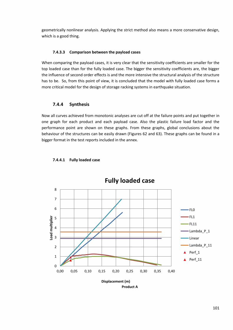
101

geometrically nonlinear analysis. Applying the strict method also means a more conservative design,

which is a good thing.

7.4.3.3 Comparison between the payload cases

When comparing the payload cases, it is very clear that the sensitivity coefficients are smaller for the

top loaded case than for the fully loaded case. The bigger the sensitivity coefficients are, the bigger

the influence of second order effects is and the more intensive the structural analysis of the structure

has to be. So, from this point of view, it is concluded that the model with fully loaded case forms a

more critical model for the design of storage racking systems in earthquake situation.

7.4.4 Synthesis

Now all curves achieved from monotonic analyses are cut off at the failure points and put together in

one graph for each product and each payload case. Also the plastic failure load factor and the

performance point are shown on these graphs. From these graphs, global conclusions about the

behaviour of the structures can be easily drawn (Figures 62 and 63). These graphs can be found in a

bigger format in the test reports included in the annex.

7.4.4.1 Fully loaded case

Product A

0

1

2

3

4

5

6

7

8

0,00 0,05 0,10 0,15 0,20 0,25 0,30 0,35 0,40

Load

mu

ltip

lier

Displacement (m)

Fully loaded case

FL0

FL1

FL11

Lambda_P_1

Linear

Lambda_P_11

Perf_1

Perf_11

102

Product B

Product C

0

0,5

1

1,5

2

2,5

3

3,5

4

4,5

0,00 0,10 0,20 0,30 0,40 0,50

Load

mu

ltip

lier

Displacement (m)

Fully loaded case

FL0

FL1

FL11

Lambda_P_1

Lambda_P_11

Linear

Perf_1

Perf_11

0

0,5

1

1,5

2

2,5

3

3,5

4

0,00 0,05 0,10 0,15 0,20 0,25 0,30

Load

mu

ltip

lier

Displacement (m)

Fully loaded case

FL0

FL1

FL11

Lambda_P_1

Linear

Lambda_P_11

Perf_1

Perf_11

103

Product D

Figure 62: Synthesis of the monotonic analyses (fully loaded case)

Legend

Linear: Linear elastic analysis;

FL0: Nonlinear elastic analysis with Hooke's law;

FL1: Nonlinear analysis with elastic-perfectly plastic law (design curve of product);

FL11: Nonlinear analysis with stepwise law for connectors (Aachen results) and elastic-

perfectly plastic law for column bases (designer's sheet);

Lambda_P_1 : Calculated corresponding to FL1;

Lambda_P_11: Calculated corresponding to FL11;

Perf_1: Performance point corresponding to FL1;

Perf_11: Performance point corresponding to FL11.

Consideration of the plastic failure load factor

In all graphs above, one can easily see that the plastic failure load factor is significantly larger than

the curve maxima for all products and material laws. This difference is primarily due to second order

effects. This observation is in accordance with the calculated interstorey drift sensitivity factors

above, as those values indicated significant second order effects.

For the comparison between the products, the factor by which the curve maximum has to be

multiplied to achieve the plastic failure load factor was calculated. These factors are summarized in

the table below (Table 22).

0

1

2

3

4

5

6

0,00 0,05 0,10 0,15 0,20 0,25

Load

mu

ltip

lier

Displacement (m)

Fully loaded case

FL0

FL1

FL11

lambda_P_1

Linear

Lambda_P_11

Perf_1

Perf_11

104

Table 22: / (fully loaded case)

Product Material law 1 Material law 11

A 2.32 3.52

B 2.26 2.57

C 4.08 5.36

D 3.67 5.48

The first conclusion that can be drawn from the table above is that a significant difference exists

between the types of analyses done. The factors for the analyses using material law 11 are bigger

than those for material law 1. This means that the influence of second order effects is bigger in

reality than expected in the design, using an elastic-perfectly plastic material law for the beam-to-

column connectors.

As the values for material law 11 are the most realistic, the comparison between the products is

based on these values. One can see that the lowest factor is seen for product B and the highest factor

for product D. Looking at the values, it is concluded that products C and D suffer the most second

order effects. Furthermore, as this plastic failure load factor is a first order measure for the maximum

plastic reserve of the structure, it is concluded that product B consumes most of its first order plastic

reserve and products C and D the least of its first order plastic reserve.

Consideration of the performance point

Evaluating the performance points on the curves for all products, one sees that all performance

points are positioned at the left side of the curve maximum. This means that all storage racking

systems are certainly able to withstand the seismic action applied on them.

When comparing the performance points for each product, it is observed that for product B the

performance point is positioned closest to the curve maximum. For the other three products, the

position of the performance point is situated in the elastic part of the curves. For these latter

products, this means that the storage rack still behaves elastic when providing the seismic

displacement demand. It is concluded that these three products are conservatively (over)designed

for the applied seismic action. For product B, the performance point is situated well in the plastic

zone of the curve, resulting in the conclusion that this storage racking system is designed more

optimal for the applied seismic action.

It is mentioned that due to the choice of another response spectrum and seismicity system for

product B, the target displacement has a very high value in comparison with the other three

products.

105

Consideration of the displacement upon first component failure

For this payload case, the first component that failed was the interior column base. This was the case

for all products.

For product B, one sees that the cut-off point is very close to the curve maximum and that the load

multiplier is significantly different for both material laws. For the other products, the cut-off point is

located a bit further away from the curve maximum and for both material laws the load multiplier is

almost the same.

For comparison, the maxima and the cut-off points for each product are summarized in the table

below. As the analysis with material law 11 is the most realistic one, only these values are given

below (Table 23).

Table 23: Ductility (fully loaded case)

Product Curve maximum Cut-off point

Displacement (m) Load multiplier Displacement (m) Load multiplier

A 0.15 1.01 0.36 0.11 0.21

B 0.37 1.02 0.42 1.01 0.05

C 0.14 0.70 0.26 0.51 0.12

D 0.15 0.95 0.23 0.86 0.08

By determining the difference in deformation between the maxima and the failure points of the

pushover curves, an approximate evaluation of the ductility of each product can be performed. From

these difference values, it is concluded that product A exhibits the most ductility. The least ductility is

observed for products B and D. The possession of a significant ductility is a benefit as failure happens

more gradually. For the case of storage racking systems, this ductility could give surrounding people

more time to evacuate before the first component of the system fails, which is most likely followed

by partial or total collapse of the system.

106

7.4.4.2 Top loaded case

Product A

Product B

0

5

10

15

20

25

30

0,00 0,10 0,20 0,30 0,40 0,50 0,60 0,70 0,80 0,90

Load

mu

ltip

lier

Displacement (m)

Top loaded case

TL0

TL1

TL11

Lambda_P_1

Linear

Lambda_P_11

Perf_1

Perf_11

0

2

4

6

8

10

12

14

16

0,00 0,10 0,20 0,30 0,40 0,50 0,60 0,70 0,80 0,90 1,00 1,10

Load

mu

ltip

lier

Displacement (m)

Top loaded case

TL0

TL1

TL11

Lambda_P_1

Lambda_P_11

Linear

Perf_1

Perf_11

107

Product C

Product D

Figure 63: Synthesis of the monotonic analyses (top loaded case)

0

2

4

6

8

10

12

14

16

18

20

0,00 0,10 0,20 0,30 0,40 0,50 0,60 0,70

Load

mu

ltip

lier

Displacement (m)

Top loaded case

TL0

TL1

TL11

Lambda_P_1

Linear

Lambda_P_11

Perf_1

Perf_11

0

5

10

15

20

25

30

0,00 0,10 0,20 0,30 0,40 0,50 0,60 0,70

Load

mu

ltip

lier

Displacement (m)

Top loaded case

TL0

TL1

TL11

Lambda_P_1

Linear

Lambda_P_11

Perf_1

Perf_11

108

Legend

Linear: Linear elastic analysis;

TL0: Nonlinear elastic analysis with Hooke's law;

TL1: Nonlinear analysis with elastic-perfectly plastic law (design curve of product);

TL11: Nonlinear analysis with stepwise law for connectors (Aachen results) and elastic-

perfectly plastic law for column bases (designer's sheet);

Lambda_P_1 : Calculated corresponding to TL1;

Lambda_P_11: Calculated corresponding to TL11;

Perf_1: Performance point corresponding to TL1;

Perf_11: Performance point corresponding to TL11.

Consideration of the plastic failure load factor

As was the case for the fully loaded condition, all plastic failure load factors are situated well above

the curve maxima. Again, this is in accordance with the calculated interstorey drift sensitivity factors

that indicated a significant influence of second order effects.

Similarly to the fully loaded case, the factors are calculated for the top loaded case and are

summarized in the table below (Table 24).

Table 24: / (top loaded case)

Product Material law 1 Material law 11

A 1.25 1.60

B 1.25 1.37

C 1.50 1.68

D 1.47 1.84

Evaluating the values in the table above, a lot of similarity is seen with the fully loaded case when

comparing the products. Also in the top loaded case, the values for material law 11 are larger than

for material law 1, resulting in the same conclusion as in the section above. Furthermore, the lowest

value is also here observed for product B and the highest for product D. So, for this payload case, the

same conclusions are drawn with respect to plastic reserve and influence of second order effects as

for the fully loaded case.

Consideration of the performance point

Similarly to the fully loaded case, the performance points are all situated at the left side of the curve

maxima, resulting in the conclusion that all storage racks are able to withstand the applied seismic

action.

109

When evaluating the position of the performance points on the pushover curves, one sees that for

products A, C and D the performance points are situated in the elastic range of the curves. So, also

for the top loaded case, these three products are conservatively designed or even overdesigned. For

product B, the performance points are situated close to the 'elastic limit' of the curve. So, also this

product is conservatively designed for the applied seismic action. But, when comparing the products,

it is concluded that product B has the most optimal design for its seismic action.

As in the fully loaded case, the target displacement value for product B is much larger than the values

for the other products, but this is due to the different choice of response spectrum and seismicity

system.

Consideration of the displacement upon first component failure

For the top loaded case, the first components that failed were the following:

Product A: all first level and some second level connectors;

Product B: interior base plate and two top level connectors;

Product C: interior base plate;

Product D: interior base plate;

This outcome makes sense as the column base design moments for products C and D were low when

comparing them with the design moments for products A and B (See table 8). From this outcome, it

seems that the column base design moments for these latter products are sufficient so that failure of

beam-to-column connectors is observed prior to column base failure.

Furthermore, one sees that the cut-off points reach different load multiplier values for the different

material laws. For the top loaded case, this phenomenon is observed for all products.

From a first view, it is observed that the failure points are situated close to the curve maxima for

products C and D. For the other two products, the failure points are situated further away from the

maxima. Similarly to the fully loaded case, a table is given below illustrating ductility considerations

using data from the nonlinear analyses with material law 11 (Table 25).

Table 25: Ductility (top loaded case)

Product Curve maximum Cut-off point

Displacement (m) Load multiplier Displacement (m) Load multiplier

A 0.32 6.80 0.89 2.94 0.57

B 0.53 3.72 0.96 3.34 0.43

C 0.55 6.71 0.68 6.48 0.13

D 0.49 8.12 0.67 7.69 0.18

Considering the values in the table above, products A and B exhibit a significantly larger ductility than

the other two products.

110

7.4.4.3 Comparison between the payload cases

Consideration of the plastic failure load factor

When comparing both payload cases, a lot of similarities are observed:

All plastic failure load factors are higher than their corresponding curve maxima;

Product B possesses the lowest / factors and product D the highest.

From these observations, it is concluded that all storage racking structures suffer significant influence

from second order effects. This influence turns out to have the least effect on product B and the

most effect on product D.

When globally comparing the values in both tables, it is seen that the values for the top loaded case

are smaller than their counterparts in the fully loaded case, resulting in the conclusion that less

second order effects are observed in the top loaded case. This is in accordance with the calculated

interstorey drift sensitivity factors (See tables 18 and 21). The outcome is quite logical as the second

order effects are mainly governed by the payload and less payload is present in the top loaded case.

Consideration of the performance point

From this point of view, it is concluded that for products A, C and D, the performance points are all

situated in the elastic zone of the pushover curve, for both payload cases. For product B, the

performance point is situated in the plastic zone of the pushover curve for the fully loaded case and

in the elastic zone (elastic limit) for the top loaded case.

Furthermore, it is observed that the target displacement values for the top loaded case are smaller

than those for the fully loaded case. As a result, one can conclude that from this point of view the

fully loaded case is a more critical payload case for design considerations as the seismic demand is

bigger for the same storage racking system and seismic event.

Consideration of the displacement upon first component failure

For products A and B, difference is observed in which components are first failing. For the fully

loaded case these components are the interior base plates. For the top loaded case, also beam-to-

column connectors are involved.

More difference between the use of the material laws is observed for the top loaded case,

considering the load multiplier values at the cut-off points.

When comparing the cut-off points from both payload cases for each product, it is observed that the

displacements and corresponding total shear loads reach higher values for the top loaded case.

From comparing ductility considerations, product C shows the same ductility for both payload cases,

whereas product A possesses a larger ductility in the top loaded case than in the fully loaded case.

Furthermore, this product has the largest ductility among all products for both payload cases.

Product B shows the lowest ductility in the fully loaded case, but has a significant ductility in the top

loaded case. Product D also has a low ductility in the fully loaded case and an intermediate ductility

in the top loaded case.

111

Overally, the storage racking systems show more ductility when tests are performed for the top

loaded case. As a result, it is concluded that the fully loaded case forms a more critical condition for

the design of storage racking systems.

7.5 Cyclic and dynamic analyses for product B

As stated in Chapter 5, the cyclic and dynamic analyses are included in this dissertation for illustrative

reasons only. These analyses were only performed for product B and for the fully loaded case. The

choice for this product and payload case was done after evaluating the monotonic test results. For

this specific case, the performance point was situated in the plastic zone of the pushover curve. In

what follows, the test results for the cyclic and dynamic analyses are illustrated.

7.5.1 Cyclic analyses

For both nonlinear material laws, the test results from the cyclic analysis are shown together with

the respective pushover curves (Figures 64 and 65). To do so, the total base shear force was

calculated and put on the vertical axis of the graphs.

7.5.1.1 Nonlinear analysis with elastic-perfectly plastic material law

Figure 64: Cyclic vs. Monotonic (Material law 1)

-6,0

-5,0

-4,0

-3,0

-2,0

-1,0

0,0

1,0

2,0

3,0

4,0

5,0

6,0

-0,50 -0,40 -0,30 -0,20 -0,10 0,00 0,10 0,20 0,30 0,40 0,50

Tota

l bas

e s

he

ar f

orc

e (

kN)

Displacement (m)

Cyclic vs. Monotonic (law 1)

C1

FL1

112

From the graph above, a good fit is observed between both analyses. The slope of the cyclic curves is

approximate the same as the initial slope of the monotonic curve when passing through (or close to)

the origin. Furthermore, when the displacement is growing to 0.30 m and 0.40 m, the base shear

force values at these points are almost the same for both analyses. A higher maximum base shear

force is reached in the cyclic analysis than in the monotonic analysis and this maximum is reached at

a smaller displacement.

It is mentioned that the negative displacement part of the graph is not representative for the

behaviour of the storage racking system because of current limitations of FineLg[13] in the

implementation of material law 1 for cyclic tests. In reality, the curves should exhibit a more point-

symmetrical behaviour.

7.5.1.2 Nonlinear analysis with piecewise linear material law

Figure 65: Cyclic vs. Monotonic (Material law 11)

As was the case for the analysis with the elastic-perfectly plastic material law, a good fit is seen

between both analyses. The same observations as in the former graph are present here. Also the

same remark is valid here about the left part of the graph.

-6,0

-5,0

-4,0

-3,0

-2,0

-1,0

0,0

1,0

2,0

3,0

4,0

5,0

6,0

7,0

Tota

l bas

e s

he

ar f

orc

e (

kN)

Displacement (m)

Cyclic vs. Monotonic (law 11)

C11

FL11

113

7.5.1.3 Comparison between both material laws

For both cases, a good fit is observed between the monotonic and cyclic analyses. Furthermore, one

sees that the maximum force in the cyclic analyses is higher for 'law 11' than for 'law 1' and that this

maximum is situated at a higher displacement value for law '11'. So, as was the case in the

monotonic analyses, it is concluded that the real storage racking systems possess a higher seismic

resistance than expected from design, resulting in a conservative design.

7.5.2 Dynamic analyses

As these analyses are only meant for illustrative reasons, only time-displacement curves are shown

below to give an idea about the behaviour of the storage rack and to compare between the used

material laws. In the figure below, the used set of ground accelerations is given (Figure 66).

Figure 66: Set of ground accelerations

7.5.2.1 Elastic analysis

Similar to the tests performed in the monotonic analyses, the linear elastic analysis assumed that all

rotation springs behaved according to Hooke's law. So no yielding could occur in this type of analysis.

The figure below shows the displacement in time of the central top node of the storage rack when

the set of ground accelerations above was applied (Figure 67).

-2,5

-2

-1,5

-1

-0,5

0

0,5

1

1,5

2

2,5

0 2 4 6 8 10 12 14 16 18 20 22

Acc

ele

rati

on

[m

/s²]

Time [s]

Set of accelerations

Accelerations

114

Figure 67: Elastic analysis

7.5.2.2 Nonlinear analyses with plastic zone

Now, the test was run assuming plastic zones for the rotation springs. Material laws 1 and 11 were

used. Figure 68 below illustrates the time-displacement behaviour for both material laws.

Figure 68: Nonlinear analyses with plastic zone

0

2

4

6

8

10

12

14

16

18

20

22

-0,4 -0,3 -0,2 -0,1 0 0,1 0,2 0,3 0,4

Tim

e [

s]

Displacement [m]

Elastic analysis

D0

0

2

4

6

8

10

12

14

16

18

20

22

-0,20 -0,15 -0,10 -0,05 0,00 0,05 0,10 0,15 0,20

Tim

e [

s]

Displacement [m]

Nonlinear analysis with plastic zone

D1

D11

115

From the figure above, it can be observed that the structure exhibits similar behaviour for both

material laws. Initially, both curves even overlap each other. Furthermore, one sees that the

maximum displacement for the analysis with material law 11 is bigger than for the other material

law. As the displacements stayed within certain limits during the test, it is concluded that no failure

of the system has occurred.

7.5.2.3 Synthesis

Now, all three analyses are put together in one graph in order to visualize the effect of plastic

deformation of the connections of the storage racking system on the behaviour of the system (Figure

69).

Initially, all graphs coincide and thus show the same behaviour. At a time of 8 seconds differences

between the curves start to appear. Then, at a time of about 12 seconds, much larger displacements

are detected for the elastic curve than for the other ones. Also, the displacements of the curves are

in opposite directions for some given values of time. From this phenomenon, it is concluded that

connections have yielded, resulting in significant damping of the system. As a result of this damping

effect, maximum displacements are reduced with a factor of 2 and the system is reacting slower.

Figure 69: Synthesis

0

2

4

6

8

10

12

14

16

18

20

22

-0,30 -0,25 -0,20 -0,15 -0,10 -0,05 0,00 0,05 0,10 0,15 0,20 0,25 0,30

Tim

e [

s]

Displacement [m]

Nonlinear analysis with plastic zone

D1

D11

D0

116

8. Conclusions

As part of the SEISRACKS 2-project, numerical testing was performed on four products with the

software package FineLg[13]. For each product, two payload cases were preconceived: a fully loaded

case and a top loaded case. Products A, C and D were storage racking systems meant for low seismic

action and were designed for a type 2 response spectrum and soil class C. Product B was meant for

high seismic action and was designed for a type 1 response spectrum and soil class C.

The modal analysis resulted in high values for the first period for all products and payload cases. Only

for product B in the top loaded case, the first period was smaller than TD of the elastic response

spectrum. The payload has a significant influence on the modes, as the fully loaded case resulted in

the higher period values. Products A and B exhibited the lowest periods in both payload cases, as

these systems are more stiff than the other two. For the fully loaded case, the percentage of

collaborate mass of the first period is about 85 % and is assumed to be sufficient for the calculation

of the seismic action. For the top loaded case, this percentage is off course 100 % as there is only one

mode for this model.

The calculation of the seismic action resulted in much higher values for product B in both payload

cases. This is mainly due to the use of a type 1 response spectrum instead of a type 2 and the use of a

higher design ground acceleration as this system is meant for high seismic action. The values for the

other three products lie closer to each other, the lowest being for product A.

The monotonic analyses resulted in the following conclusions.

From the elastic analyses, it is concluded that the nonlinear behaviour of storage racking systems is

governed by the payload and the overall stiffness of the system. The degree of nonlinearity was

bigger for the fully loaded case than for the top loaded case as more payload was applied in this first

case. As products A and B are more stiff than the other two, the degree of nonlinear behaviour was

smaller in both payload cases. Moreover, when the overall stiffness of the system is high, the

influence of the payload on the nonlinearity is smaller than when the overall stiffness is low. When

the payload is high (fully loaded case), the influence of the overall stiffness of the system on the

nonlinearity is larger than when the payload is low (top loaded case).

From the nonlinear analyses with plastic zone, it is concluded that all products exhibited the same

overall behaviour regardless of the payload case. This behaviour is translated through an overall

shape of the pushover curve. First, an approximate linear ascending part of the curve is observed

illustrating elastic behaviour. This part is followed by a straight, sometimes curved, ascending part

where some components (mostly the column bases) already have yielded, but where the elastic

behaviour of the remaining not yielded components (beam-to-column connectors) is sufficient to

resist the momentary seismic load. Then, the maximum load is reached. At this point, some vital

components have yielded so that the system could no longer resist the applied load. Beyond this

point, the pushover curve is descending, meaning that less load is needed to further deform the

structure. In reality, the descending part will stop where the components start to fail, as the storage

racking system will partly or completely fail beyond this point.

117

Considering displacement values on the pushover curves, it is concluded that the real storage racking

systems allow more deformation to occur before the maximum load is reached than is assumed in

their design. The highest displacement values were exhibited by product B in both payload cases. For

the other three products, the displacements corresponding to the curve maxima are approximate the

same and significantly lower than those of product B in the fully loaded case. For the top loaded case,

the displacements are approximate the same for products B, C and D and are lower for product A.

The reached displacements are larger for the top loaded case than for the fully loaded case.

Considering load multiplier values, it is concluded that for products A, C and D in the fully loaded case

the realistic model (material law 11) shows a slight understrength but better plastic behaviour after

reaching the curve maximum, when comparing with the material law 1 model. For product B in the

fully loaded case and all four products in the top loaded case, the realistic model shows a slight

overstrength and same plastic behaviour after reaching the curve maximum. Furthermore, the

maximum base shear force reached by the systems is larger for the top loaded case than the fully

loaded case. The difference is smallest for products A and B, and highest for products C and D,

indicating that the influence of the payload condition on the maximum base shear force is smaller for

systems with higher stiffness.

Considering the amount of energy absorbed during the tests, it is concluded that for products A, C

and D in the fully loaded case, the amount of absorbed energy is approximate the same for both

analyses (material law 1 and 11). For product B in the fully loaded case and all products in the top

loaded case, the absorbed energy is larger for the more realistic model than for the material law 1

model. Furthermore, product B absorbs the most energy in both payload cases, proving that this

system is indeed a high seismicity system. Finally, more energy is absorbed in the top loaded case

than in the fully loaded case for all products.

From the calculation of the interstorey drift sensitivity factors it is concluded that for both payload

cases the maximum values are found for the first storey of each product. Moreover, the absolute

maximum values are found for product D and the lowest are found for products A and B. As a result,

it is stated that the larger the systems overall stiffness, the smaller the sensitivity factors and the

smaller the impact of second order effects will be. In the fully loaded case, the second order effects

are largest for the first storey and lowest for the top storey. In the top loaded case, the second order

effects are evenly distributed among the storeys. Considering the comparison with table 5 adopted

from FEM 10.2.08[2], it is concluded that in the fully loaded case, the second order effects must be

explicitly considered in the analysis through geometrically nonlinear analysis for all products.

Furthermore, it is recommended that products C and D are reinforced through horizontal bracing in

order to make these systems more stiff. In the top loaded case it is concluded that for products A, B

and C, second order effects can be approximately taken into account by multiplying the relevant

seismic action by a factor of 1/(1- ). For product D, the same is true for the top storeys. For the

first storey it is conservative to perform a geometrically nonlinear analysis. Finally it is stated that the

top loaded case suffers less second order effects than the fully loaded case.

When considering the plastic failure load factors, it is concluded that all products suffer second order

effects in both payload cases. Furthermore, it is stated that second order effects have a bigger impact

in the real storage racking system (analysis with law 11) than in the design system (analysis with law

1). It is concluded that products C and D suffer most second order effects and product B the least in

118

both payload cases. Finally, all top loaded models suffered less second order effects than their fully

loaded counterparts.

From the examination of the performance point, it is observed that all performance points are

situated at the left side of the curve maxima. As a result, it is concluded that all products meet the

seismic demand in both payload cases. Moreover, these performance points are situated in the

elastic region for products A, C and D in both payload cases and for product B in the top loaded case,

resulting in the conclusion that the design of these storage racking systems is pretty conservative for

the applied seismic action. The performance point is situated in the plastic region of the curve for

product B in the fully loaded case. Product B is most optimally designed for its seismic action in both

payload cases when comparing the four products. Finally, it is stated that the seismic demand is

bigger for the fully loaded case than the top loaded case.

Considering first component failure, it is stated that in the fully loaded case this component was

always the interior column base connection. This was also the case in the top loaded condition for

products C and D. For product A, the first components that failed in the top loaded condition were

the first level and second level beam-to-column connectors and for product B the interior base plate

and the top level connectors. In the fully loaded case, it is concluded that product A exhibited the

most and products B and D the least ductile behaviour. For the top loaded case, the most ductile

systems were products A and B. In the top loaded case, the corresponding shear load and

displacement values of the cut-off points are higher than those in the fully loaded case. Moreover,

the models in the top loaded case exhibited more ductility than those in the fully loaded case.

It is mentioned that all conclusions from all the different points of consideration above agree with

and reinforce each other. Moreover, it is indisputable that the fully loaded case is the most critical

payload case for the design of storage racking systems in earthquake situation. The overall behaviour

of the storage racking systems was the same. All storage racking systems suffered second order

effects, products C and D suffering the most. Furthermore, it is stated that for the low seismicity

products A, C and D, the overall performance of product C and D was more similar than any other

combination of products, while the performance of product A happened to be slightly better.

Moreover, the performance of product A possesses some similarities with products C and D, but also

with product B. Being a high seismicity system, product B allowed larger displacements and absorbed

more energy upon failure. Finally, it is concluded that all four types of storage racks met their seismic

demands, product B being the least conservative from this point of view and that the design of

storage racks assuming elastic-perfectly plastic material laws for the connections is conservative.

The illustrative cyclic and dynamic analyses for the fully loaded model of product B resulted in the

following conclusions.

The cyclic analyses for product B showed a good fit with the pushover curves from the monotonic

analyses. Higher maximum base shear forces and smaller corresponding displacements were reached

in the cyclic analyses when comparing them with the monotonic pushover curves. As the curve

maximum of the more realistic model is situated at higher values of the base shear force and

corresponding displacement than is the case for the 'design model', it is concluded that the design of

119

this storage racking system according to material law 1 for beam-to-column connectors is

conservative.

From the dynamic example, it is concluded that significant damping occurred as a result of the

yielding of connections between columns and floor and/or between beams and columns. The

damping effect resulted in significant reduction of horizontal displacement and time shift of the

system response to the set of ground accelerations when comparing elastic and nonlinear dynamic

analyses.

120

Annex A: Test report product A

For this product, the chosen system to be tested was the low to medium seismicity system. The

characteristics of the beams and columns are the following:

Table A.1: Component characteristics

Component A [ ] I [ ] E [ ] Beam 762.0

Column 674.0

A.1 Fully loaded model

A.1.1 Modal Analysis

Table A.2: Modes

Mode Frequence (Hz) Period (s) Percentage of Collaborate Mass (%)

1 0.447 2.235 84.169

2 1.630 0.613 11.535

3 3.579 0.279 3.519

4 6.061 0.165 0.778

5 53.659 0.019 0.000

A.1.2 Calculation of Horizontal forces

A.1.2.1 Input data

Table A.3: Input data

Parameter Value (m/s²) 1.1772

0.84 Soil type C

Type of response spectrum 2 S 1.5

(s) 0.1 (s) 0.25 (s) 1.2

0.2 q 2

(kg) 9600

0.8

1.0

121

A.1.2.2 Calculation of the base shear force

Calculation of the ordinate of the response spectrum

As :

So:

Calculation of the total mass

Calculation of the seismic base shear force

A.1.2.3 Calculation of the triangular distributed horizontal forces

Table A.4: Seismic action

Level z (m) m (kg) (kgm) F (kN) 1 1.9670 2400 4720.8 0.1515 2 3.9430 2400 9463.2 0.3036 3 5.9190 2400 14205.6 0.4558 4 7.8950 2400 18948.0 0.6080

A.1.3 Monotonic analyses

A.1.3.1 Linear elastic analysis and nonlinear elastic analysis (constitutive law 0)

Constitutive law 0 for all components;

No payload applied during linear elastic analysis;

Payload is applied during nonlinear elastic analysis.

122

Rotation spring characteristics

Table A.5: Rotation spring characteristics

Spring Stiffness k (kNm/rad) Design moment (kNm) Beam-to-column connections 139.4500 -

Interior column base 535.5840 - Exterior column base 237.0216 -

Load-displacement curves

Figure A.1: Linear elastic analysis

Figure A.2: Nonlinear elastic analysis

0

5

10

15

20

25

30

35

40

45

0 0,2 0,4 0,6 0,8 1 1,2 1,4

Load

mu

ltip

lier

Displacement (m)

FL0 Linear

FL Linear

0

10

20

30

40

50

60

70

80

0,00 0,50 1,00 1,50 2,00 2,50 3,00

Load

mu

ltip

lier

Displacement (m)

FL0 nonlinear

Pushover curve

123

A.1.3.2 Nonlinear analysis with plastic zone (Constitutive law 1)

Constitutive law 0 for beams and columns;

Constitutive law 1 for rotation springs (designer's sheets);

Payload is applied.

Rotation spring characteristics

Table A.6: Rotation spring characteristics

Spring Stiffness k (kNm/rad) Design moment (kNm) Beam-to-column connections 139.4500 1.4370

Interior column base 535.5840 1.1793 Exterior column base 237.0216 0.9617

Load-displacement curve

Figure A.3: Nonlinear analysis law 1

Course of the test

o Loading step 1-17: Linear load-displacement curve;

o Loading step 18: Interior column base yields;

o Loading step 19: Second column base (third column) and first to fourth connectors yield: first

level: second column left side and third column; second level: second column left side and

third column;

o Loading step 20: Third column base yields : first column;

All column bases have yielded

-0,4

-0,2

0

0,2

0,4

0,6

0,8

1

1,2

1,4

0,00 0,05 0,10 0,15 0,20 0,25 0,30 0,35 0,40 0,45

Load

mu

ltip

lier

Displacment

FL1

Pushover curve

124

o Loading step 21-26: Loading;

o Loading step 27: Fifth connector yields: third level: third column;

o Loading step 28: Loading;

o Loading step 29: Sixth connector yields: third level: second column left side;

o Loading step 30-34: Loading;

o Loading step 35: Seventh and eighth connectors yield: first level, first column and second

column right side;

All first level connectors have yielded

o Loading step 36: Ninth and tenth connectors yield: fourth level: second column left side and

third column;

o Loading step 37: Eleventh and Twelfth connectors yield: second level: first column and

second column right side;

All second level connectors have yielded

o Loading step 38-40: Loading;

o Loading step 41: Thirteenth and fourteenth connectors yield: third level, first column and

second column right side;

All third level connectors have yielded

o Loading step 42: Loading.

A.1.3.3 Nonlinear analysis with plastic zone (Constitutive law 11)

Constitutive law 0 for beams and columns;

Constitutive law 1 for column base rotation springs (designer's sheets);

Constitutive law 11 for beam-to-column connection rotation springs (Aachen test results);

Payload is applied.

Rotation spring characteristics

Table A.7: Rotation spring characteristics

Spring Stiffness k (kNm/rad) Design moment (kNm) Beam-to-column connections - -

Interior column base 535.5840 1.1793 Exterior column base 237.0216 0.9617

125

Figure A.4: Beam-to-column rotation springs

Pushover curve

Figure A.5: Nonlinear analysis law 11

0

0,2

0,4

0,6

0,8

1

1,2

1,4

1,6

1,8

2

0 0,01 0,02 0,03 0,04 0,05 0,06 0,07

Mo

me

nt

(kN

m)

Rotation (rad)

Stepwise function fully loaded connectors

Stepwise function

0

0,2

0,4

0,6

0,8

1

1,2

0,00 0,05 0,10 0,15 0,20 0,25 0,30 0,35 0,40

Load

mu

ltip

lier

Displacement (m)

FL11

Pushover curve

126

Course of the test

o Loading step 1-12: Linear load-displacement curve;

o Loading step 13: Interior column base yields;

o Loading step 14: Loading, deterioration of the connector stiffness;

o Loading step 15: Exterior column bases yield;

All column bases have yielded

o Loading step 16-34: Loading, deterioration of the connector stiffness;

o Loading step 35: First connector yields: First level, third column;

o Loading step 36: Second connector yields: first level, second column left side;

o Loading step 37: Loading, deterioration of the connector stiffness;

o Loading step 38: Third and fourth connectors yield: second level, second column left side and

third column;

o Loading step 39: Fifth and sixth connectors yield: first level, first column and second column

right side;

All first level connectors have yielded

o Loading step 40: Loading, deterioration of the connector stiffness;

o Loading step 41: Seventh and eighth connectors yield: second level: first column and second

column right side;

All second level connectors have yielded

o Loading step 42: Ninth and tenth connectors yield: third level, second column left side and

third column.

A.1.4 Calculation of failure rotations

For beam-to-column connectors, use is made of the moment-rotation curves adopted from

the tests conducted in Aachen (See Chapter 4);

For column bases, use is made of the SEISRACKS report[1] (page 51) (See Chapter 6);

Table A.8: Failure rotations

Connection (kNm) (kNm) (mrad) Beam-to-column 1.8400 1.4720 110

Interior column base 1.1793 0.9434 68 Exterior column base 0.9617 0.7694 87

127

A.1.4.1 Determination of the end step (cut-off point)

Nonlinear analysis law 1

Cut off at step 41 (Interior column base reaches a rotation of 69.028 mrad).

Nonlinear analysis law 11

Cut off at step 42 (Interior column base reaches a rotation of 54.299 mrad).

A.1.5 Calculation of the failure parameter

A.1.5.1 Nonlinear analysis law 1 (design curve)

A.1.5.2 Nonlinear analysis law 11 (stepwise curve)

A.1.6 Calculation of the performance point

A.1.6.1 Nonlinear analysis law 1 (design curve)

128

Transformation to an equivalent SDOF system

Determination of the idealized elastic-perfectly plastic force-displacement relationship

Determination of the period of the idealized equivalent SDOF system

Determination of the target displacement

Determination of the difference with

Second iteration

129

Corresponding shear force value calculated through linear interpolation:

Determination of the target displacement for the MDOF system

A.1.6.2 Nonlinear analysis law 11 (stepwise curve)

Normalized horizontal forces

Transformation to an equivalent SDOF system

Determination of the idealized elastic-perfectly plastic force-displacement relationship

130

Determination of the period of the idealized equivalent SDOF system

Determination of the target displacement

Determination of the difference with

Second iteration

Corresponding shear force value calculated through linear interpolation:

Determination of the target displacement for the MDOF system

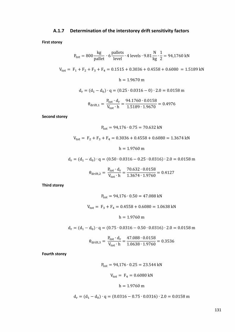
131

A.1.7 Determination of the interstorey drift sensitivity factors

First storey

Second storey

Third storey

Fourth storey

132

A.1.8 Synthesis: monotonic analyses

All monotonic curves together in one graph;

Illustration of the failure load parameter and the performance point on the graph;

Curves cut off in respect with failure rotations.

Figure A.6 : Synthesis

Legend

Linear: Linear elastic analysis;

FL0: Nonlinear analysis with Hooke's law;

FL1: Nonlinear analysis with elastic-perfectly plastic law (design curve of producer);

FL11: Nonlinear analysis with stepwise law for connectors (Aachen results) and elastic-

perfectly plastic law for column bases;

Lambda_P_1 : Calculated for design curve of the producer (FL1);

Lambda_P_11: Calculated for stepwise curve from Aachen results (FL11);

Perf_1: Performance point for FL1;

Perf_11: Performance point for FL11.

0

1

2

3

4

5

6

7

8

0,00 0,05 0,10 0,15 0,20 0,25 0,30 0,35 0,40

Load

mu

ltip

lier

Displacement (m)

Fully loaded case

FL0

FL1

FL11

Lambda_P_1

Linear

Lambda_P_11

Perf_1

Perf_11

133

A.2 Top loaded model

A.2.1 Modal Analysis

Table A.9: First mode

Mode Frequence (Hz) Period (s) Percentage of Collaborate Mass

(%)

1 0.556 1.799 100

A.2.2 Calculation of Horizontal forces

A.2.2.1 Input data

Table A.10: Input data

Parameter Value (m/s²) 1.1772

0.84 Soil type C

Type of response spectrum 2 S 1.5

(s) 0.1 (s) 0.25 (s) 1.2

0.2 q 2

(kg) 9600

0.8

1.0

A.2.2.2 Calculation of the base shear force

Calculation of the ordinate of the response spectrum

As :

Calculation of the total mass

134

Calculation of the seismic base shear force:

A.2.2.3 Calculation of the triangular distributed horizontal forces

Table A.11: Seismic action

Level z (m) m (kg) (kgm) F (kN) 1 1.9670 0 0 0 2 3.9430 0 0 0 3 5.9190 0 0 0 4 7.8950 2400 18948.0 0.3797

A.2.3 Monotonic analyses

A.2.3.1 Linear elastic analysis and nonlinear elastic analysis (Constitutive law 0)

Constitutive law 0 for all components;

No payload applied during linear elastic analysis;

Payload is applied during nonlinear elastic analysis.

Rotation spring characteristics

Table A.12: Rotation spring characteristics

Spring Stiffness k (kNm/rad) Design moment (kNm) Beam-to-column connections 139.4500 -

Interior column base 75.2682 - Exterior column base 37.6341 -

Load-displacement curves

135

Figure A.7: Linear elastic analysis

Figure A.8: Nonlinear elastic analysis

0

10

20

30

40

50

60

70

80

90

100

0 0,2 0,4 0,6 0,8 1 1,2 1,4

Load

mu

ltip

lier

Displacement (m)

TL0 Linear

TL Linear

0

20

40

60

80

100

120

140

160

0,00 0,25 0,50 0,75 1,00 1,25 1,50 1,75 2,00 2,25

Load

mu

ltip

lier

Displacement (m)

TL0 Nonlinear

Pushover curve

136

A.2.3.2 Nonlinear analysis with plastic zone (Constitutive law 1)

Constitutive law 0 for beams and columns;

Constitutive law 1 for rotation springs (designer's sheets);

Payload is applied.

Rotation spring characteristics

Table A.13: Rotation spring characteristics

Spring Stiffness k (kNm/rad) Design moment (kNm) Beam-to-column connections 139.4500 1.4370

Interior column base 75.2682 0.8148 Exterior column base 37.6341 0.7330

Load-displacement curve

Figure A.9: Nonlinear analysis law 1

Course of the test

o Loading step 1-15: Linear load-displacement curve;

o Loading step 16: Interior column base yields, first and second connectors yield: fourth level,

second column left side and third column;

o Loading step 17: Loading;

o Loading step 18: Third to sixth connectors yield: all first level connectors;

All first level connectors have yielded

0

1

2

3

4

5

6

7

8

0,00 0,10 0,20 0,30 0,40 0,50 0,60 0,70 0,80 0,90 1,00

Load

mu

ltip

lier

Displacement (m)

TL1

pushover curve

137

o Loading step 19: Seventh to tenth connectors yield: all second level connectors;

All second level connectors have yielded

o Loading step 20: Eleventh connector yields: third level, third column;

o Loading step 21: Twelfth and thirteenth connectors yield: third level, first column and second

column right side;

o Loading step 22: Fourteenth connector yields: third level, second column left side;

All third level connectors have yielded

o Loading step 23: Exterior column bases yield;

All column bases have yielded

o Loading step 24-30: Loading;

o Loading step 31: Fifteenth connector yields: fourth level, first column;

o Loading step 32: Sixteenth connector yields: fourth level, second column right side;

All connectors have yielded

o Loading step 33-42: Loading.

A.2.3.3 Nonlinear analysis with plastic zone (Constitutive law 11)

Constitutive law 0 for beams and columns;

Constitutive law 1 for column base rotation springs (designer's sheets);

Constitutive law 11 for beam-to-column connection rotation springs (Aachen test results);

Payload is applied.

Rotation spring characteristics

Table A.14: Rotation spring characteristics

Spring Stiffness k (kNm/rad) Design moment (kNm) Beam-to-column connections - -

Interior column base 75.2682 0.8148 Exterior column base 37.6341 0.7330

138

Figure A.10: Beam-to-column rotation springs

Figure A.11: Beam-to-column rotation springs

0

0,2

0,4

0,6

0,8

1

1,2

1,4

1,6

1,8

2

0 0,01 0,02 0,03 0,04 0,05 0,06 0,07

Mo

me

nt

(kN

m)

Rotation (rad)

Stepwise function fully loaded connectors

Stepwise function

0

0,5

1

1,5

2

2,5

0 0,01 0,02 0,03 0,04 0,05 0,06 0,07 0,08 0,09

Mo

me

nt

(kN

m)

Rotation (rad)

Stepwise function unloaded connectors

Stepwise function

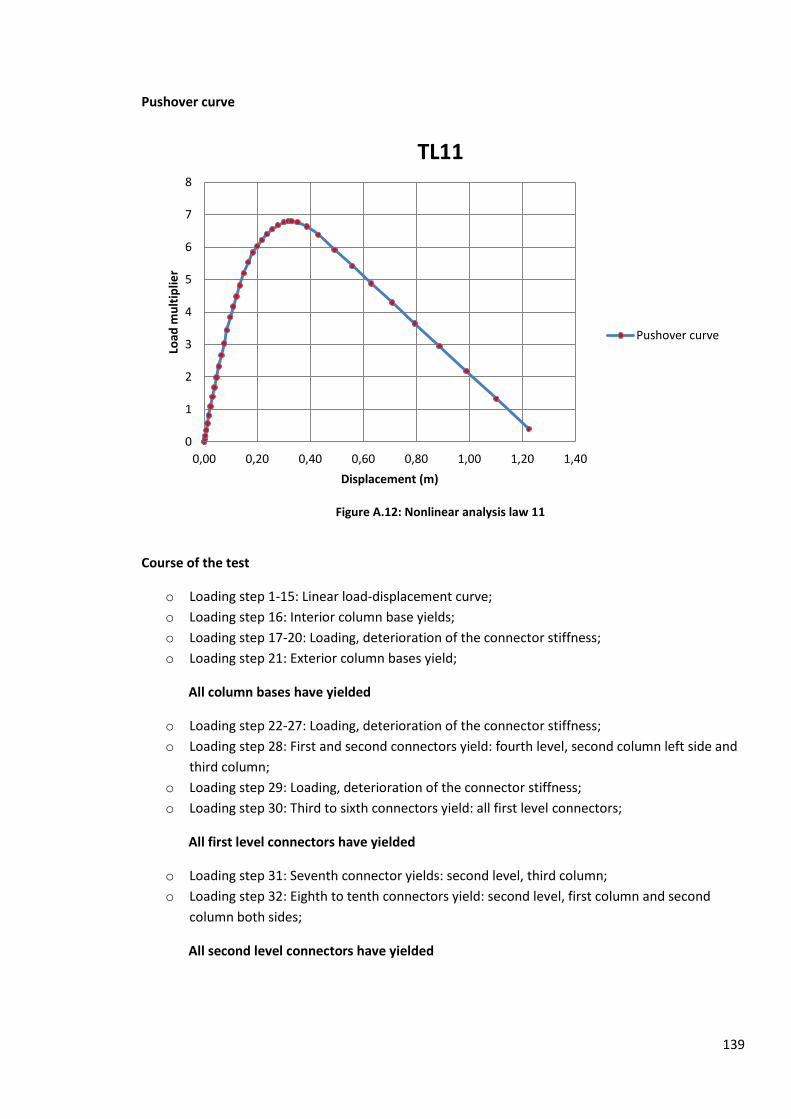
139

Pushover curve

Figure A.12: Nonlinear analysis law 11

Course of the test

o Loading step 1-15: Linear load-displacement curve;

o Loading step 16: Interior column base yields;

o Loading step 17-20: Loading, deterioration of the connector stiffness;

o Loading step 21: Exterior column bases yield;

All column bases have yielded

o Loading step 22-27: Loading, deterioration of the connector stiffness;

o Loading step 28: First and second connectors yield: fourth level, second column left side and

third column;

o Loading step 29: Loading, deterioration of the connector stiffness;

o Loading step 30: Third to sixth connectors yield: all first level connectors;

All first level connectors have yielded

o Loading step 31: Seventh connector yields: second level, third column;

o Loading step 32: Eighth to tenth connectors yield: second level, first column and second

column both sides;

All second level connectors have yielded

0

1

2

3

4

5

6

7

8

0,00 0,20 0,40 0,60 0,80 1,00 1,20 1,40

Load

mu

ltip

lier

Displacement (m)

TL11

Pushover curve

140

o Loading step 33: All remaining connectors yield;

All connectors have yielded

o Loading step 34-42: Loading.

A.2.4 Calculation of failure rotations

For beam-to-column connectors, use is made of the moment-rotation curves adopted from

the tests conducted in Aachen (See Chapter 4);

For column bases, use is made of the SEISRACKS report[1] (page 51) (See Chapter 6);

Table A.15: Failure rotations

Connection (kNm) (kNm) (mrad) Beam-to-column fully loaded 1.8400 1.4720 110 Beam-to-column unloaded 2.0000 1.6000 104

Interior column base 0.8148 0.6518 133 Exterior column base 0.7330 0.5864 160

A.2.4.1 Determination of the end step (cut-off point)

Nonlinear analysis law 1

Cut off at step 41 (all connectors of the first level reached the failure rotation: first column: 107

mrad; second column left side: 105.85 mrad; second column right side: 105.91 mrad and third

column: 107.07 mrad).

Nonlinear analysis law 11

Cut off at step 42 (all connectors of the first level are close to reaching the failure rotation: max

rotation = 99.008 mrad).

A.2.5 Calculation of the failure parameter

A.2.5.1 Nonlinear analysis law 1 (design curve)

141

A.2.5.2 Nonlinear analysis law 11 (stepwise curve)

A.2.6 Calculation of the performance point

A.2.6.1 Nonlinear analysis law 1 (design curve)

Normalized horizontal forces

Transformation to an equivalent SDOF system

Notice: This is already a single degree of freedom system!!!

Determination of the idealized elastic-perfectly plastic force-displacement relationship

Determination of the period of the idealized equivalent SDOF system

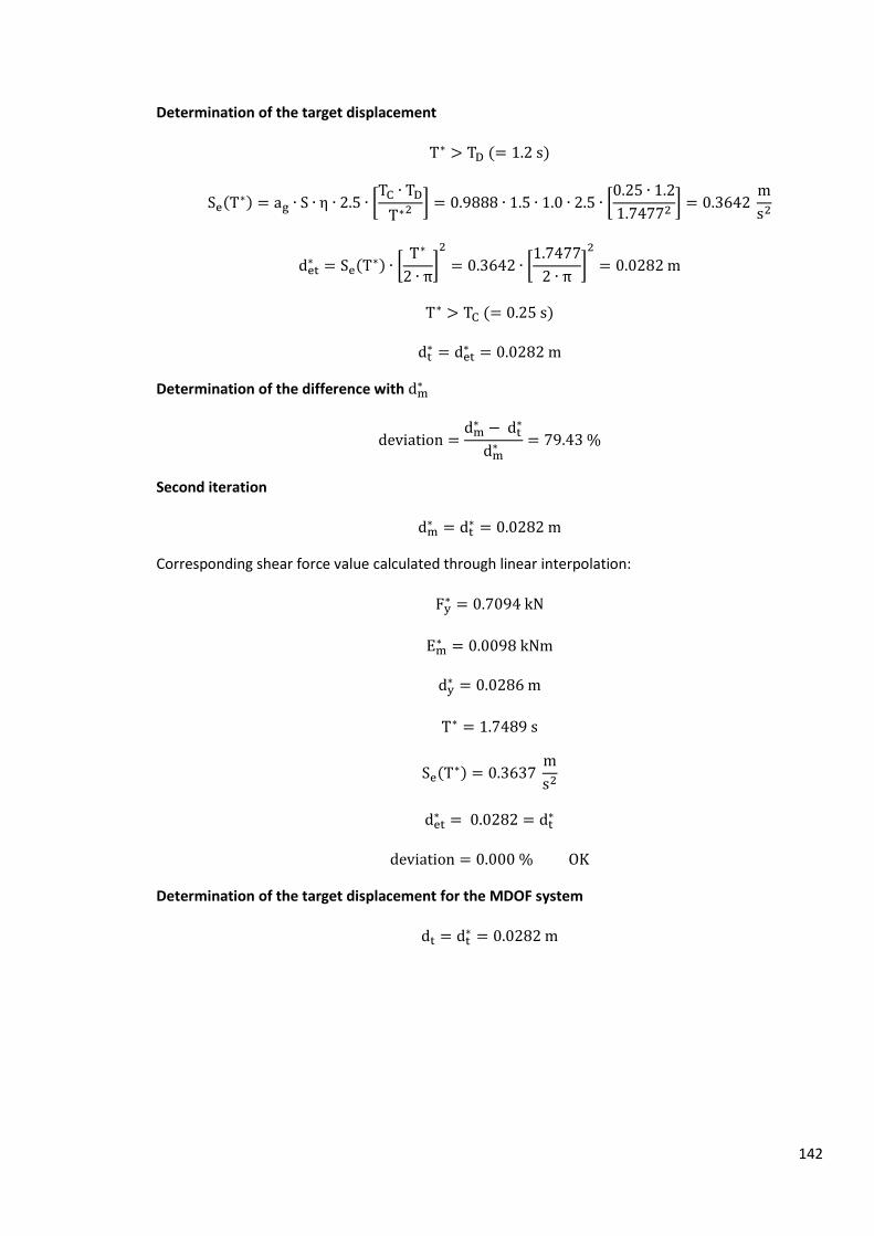
142

Determination of the target displacement

Determination of the difference with

Second iteration

Corresponding shear force value calculated through linear interpolation:

Determination of the target displacement for the MDOF system

143

A.2.6.2 Nonlinear analysis law 11 (stepwise curve)

Normalized horizontal forces

Transformation to an equivalent SDOF system

Notice: This is already a single degree of freedom system!!!

Determination of the idealized elastic-perfectly plastic force-displacement relationship

Determination of the period of the idealized equivalent SDOF system

Determination of the target displacement

144

Determination of the difference with

Second iteration

Corresponding shear force value calculated through linear interpolation:

Determination of the target displacement for the MDOF system

A.2.7 Determination of the interstorey drift sensitivity factors

First storey

145

Second storey

As no difference exists in the values for the second, third and fourth storey, the latter two storeys

have the same -value.

Third storey

Fourth storey

A.2.8 Synthesis: monotonic analyses

All monotonic curves together in one graph;

Illustration of the failure load parameter and the performance point on the graph;

Curves cut off in respect with failure rotations.

146

Figure A.13 : Synthesis

Legend

Linear: Linear elastic analysis;

TL0: Nonlinear analysis with Hooke's law;

TL1: Nonlinear analysis with elastic-perfectly plastic law (design curve of producer);

TL11: Nonlinear analysis with stepwise law for connectors (Aachen results) and elastic-

perfectly plastic law for column bases;

Lambda_P_1 : Calculated for design curve of the producer (TL1);

Lambda_P_11: Calculated for stepwise curve from Aachen results (TL11);

Perf_1: Performance point for TL1;

Perf_11: Performance point for TL11.

0

2,5

5

7,5

10

12,5

15

17,5

20

22,5

25

27,5

0,00 0,10 0,20 0,30 0,40 0,50 0,60 0,70 0,80 0,90

Load

mu

ltip

lier

Displacement (m)

Top loaded case

TL0

TL1

TL11

Lambda_P_1

Linear

Lambda_P_11

Perf_1

Perf_11

147

Annex B: Test report product B

For this product, the chosen system to be tested was the high seismicity system. The characteristics

of the beams and columns are the following:

Table B.1: Component characteristics

Component A [ ] I [ ] E [ ] Beam 686.0

Column 720.0

B.1 Fully loaded model

B.1.1 Modal Analysis

Table B.2: Modes

Mode Frequence (Hz) Period (s) Percentage of Collaborate Mass (%)

1 0.435 2.297 85.351

2 1.670 0.599 10.931

3 3.874 0.258 3.072

4 6.808 0.147 0.646

5 51.155 0.020 1.899E-18

B.1.2 Calculation of Horizontal forces

B.1.2.1 Input data

Table B.3: Input data

Parameter Value (m/s²) 2.4525

0.84 Soil type C

Type of response spectrum 1 S 1.15

(s) 0.2 (s) 0.6 (s) 2.0

0.2 q 2.0

(kg) 9600

0.8

1.0

148

B.1.2.2 Calculation of the base shear force

Calculation of the ordinate of the response spectrum

As :

So:

Calculation of the total mass

Calculation of the seismic base shear force

B.1.2.3 Calculation of the triangular distributed horizontal forces

Table B.4: Seismic action

Level z (m) m (kg) (kgm) F (kN) 1 1.945 2400 4668 0.5088 2 3.945 2400 9468 1.0319 3 5.945 2400 14268 1.5551 4 7.945 2400 19068 2.0782

B.1.3 Monotonic analyses

B.1.3.1 Linear elastic analysis and nonlinear elastic analysis (constitutive law 0)

Constitutive law 0 for all components;

No payload applied during linear elastic analysis;

Payload is applied during nonlinear elastic analysis.

149

Rotation spring characteristics

Table B.5: Rotation spring characteristics

Spring Stiffness k (kNm/rad) Design moment (kNm) Beam-to-column connections 170.601 -

Interior column base 297.558 - Exterior column base 135.326 -

Load-displacement curves

Figure B.1:Linear elastic analysis

Figure B.2: Nonlinear elastic analysis

0

2

4

6

8

10

12

0 0,2 0,4 0,6 0,8 1 1,2

Load

mu

ltip

lier

Displacement (m)

FL0 Linear

FL Linear

0

10

20

30

40

50

60

70

0,00 1,00 2,00 3,00 4,00 5,00 6,00

Load

mu

ltip

lier

Displacement (m)

FL0 nonlinear

Pushover curve

150

B.1.3.2 Nonlinear analysis with plastic zone (Constitutive law 1)

Constitutive law 0 for beams and columns;

Constitutive law 1 for rotation springs (designer's sheets);

Payload is applied.

Rotation spring characteristics

Table B.6: Rotation spring characteristics

Spring Stiffness k (kNm/rad) Design moment (kNm) Beam-to-column connections 170.601 3.4050

Interior column base 297.558 2.4333 Exterior column base 135.326 1.3490

Load-displacement curve

Figure B.3: Nonlinear analysis law 1

Course of the test

o Loading step 1-18 : Linear load-displacement curve;

o Loading step 19: All column bases yield;

All column bases have yielded

0

0,1

0,2

0,3

0,4

0,5

0,6

0,7

0,8

0,9

1

0,00 0,20 0,40 0,60 0,80 1,00

Load

mu

ltip

lier

Displacement (m)

FL1

Pushover curve

151

o Loading step 20: Loading;

o Loading step 21: first and second connectors yield: first level, second column left side and

third column;

o Loading step 22-23: Loading;

o Loading step 24: third and fourth connectors yield: second level, second column left side and

third column;

o Loading step 25-30: Loading;

o Loading step 31: fifth and sixth connectors yield: third level, second column left side and

third column;

o Loading step 32-34: Loading;

o Loading step 35: seventh and eighth connectors yield: first level, first column and second

column right side;

All first level connectors have yielded

o Loading step 36: ninth and tenth connectors yield: fourth level, second column left side and

third column;

o Loading step 37: eleventh and twelfth connectors yield: second level, first column and

second column right side;

All second level connectors have yielded

o Loading step 38-39: Loading;

o Loading step 40: thirteenth and fourteenth connectors yield: third level, first column and

second column right side;

All third level connectors have yielded

o Loading step 41: Loading;

o Loading step 42: All remaining connectors yield.

All connectors have yielded

B.1.3.3 Nonlinear analysis with plastic zone (Constitutive law 11)

Constitutive law 0 for beams and columns;

Constitutive law 1 for column base rotation springs (designer's sheets);

Constitutive law 11 for beam-to-column connection rotation springs (Aachen test results);

Payload is applied.

Rotation spring characteristics

Table B.7: Rotation spring characteristics

Spring Stiffness k (kNm/rad) Design moment (kNm) Beam-to-column connections - -

Interior column base 297.558 2.4333 Exterior column base 135.326 1.3490

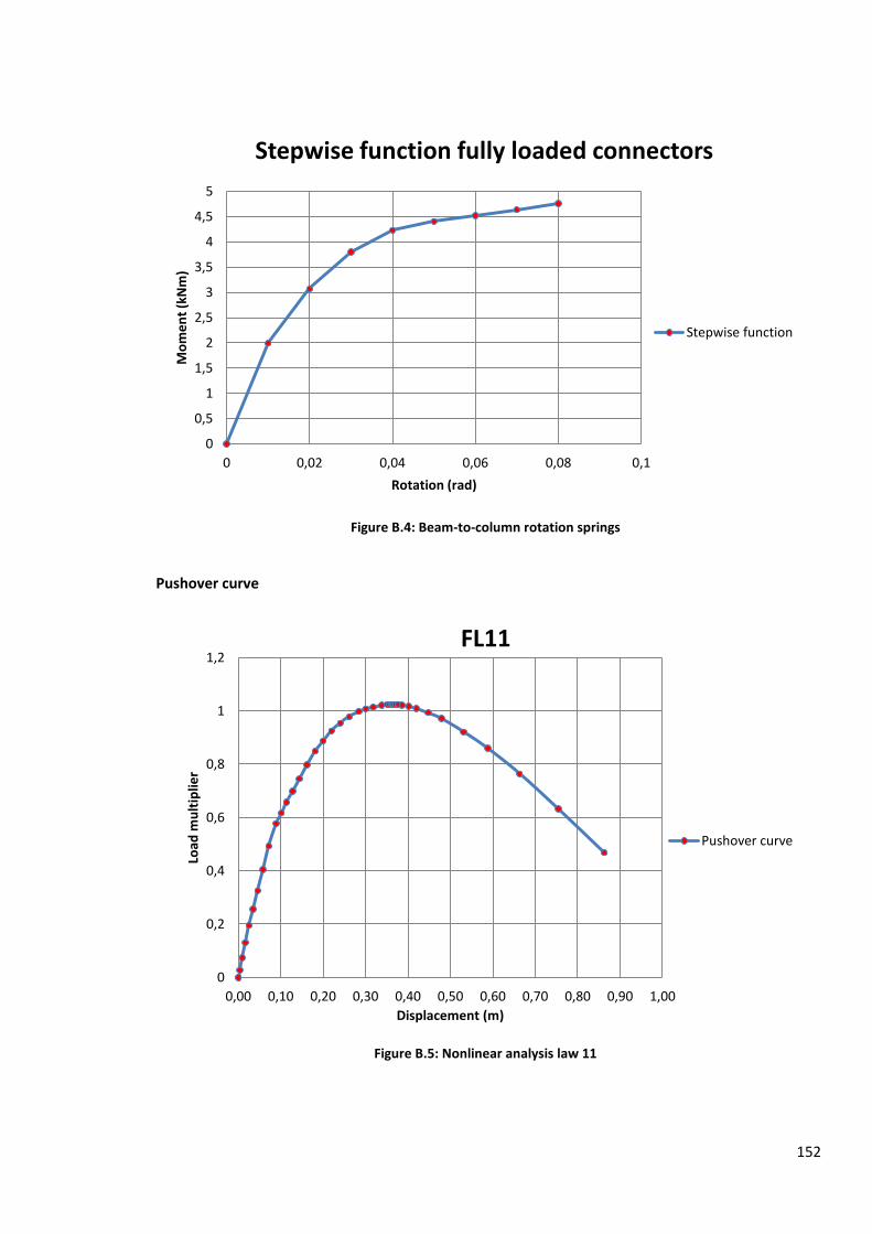
152

Figure B.4: Beam-to-column rotation springs

Pushover curve

Figure B.5: Nonlinear analysis law 11

0

0,5

1

1,5

2

2,5

3

3,5

4

4,5

5

0 0,02 0,04 0,06 0,08 0,1

Mo

me

nt

(kN

m)

Rotation (rad)

Stepwise function fully loaded connectors

Stepwise function

0

0,2

0,4

0,6

0,8

1

1,2

0,00 0,10 0,20 0,30 0,40 0,50 0,60 0,70 0,80 0,90 1,00

Load

mu

ltip

lier

Displacement (m)

FL11

Pushover curve

153

Course of the test

o Loading step 1-10: Linear load-displacement curve;

o Loading step 11: All column bases yield;

All column bases have yielded

o Loading step 12-21: Loading, deterioration of the connector stiffness;

o Loading step 22: first and second connectors yield: first level, second column left side and

third column;

o Loading step 23-31: Loading, deterioration of the connector stiffness;

o Loading step 32: third connector yields: second level, third column;

o Loading step 33: fourth connector yields: second level, second column left side;

o Loading step 34-36: Loading, deterioration of the connector stiffness;

o Loading step 37: fifth and sixth connectors yield: first level, first column and second column

right side;

All first level connectors have yielded

o Loading step 38-39: Loading, deterioration of the connector stiffness;

o Loading step 40: seventh to tenth connectors yield: second level: first column and second

column right side; third level: second column left side and third column;

All second level connectors have yielded

o Loading step 41: Loading, deterioration of the connector stiffness;

o Loading step 42: eleventh connector yields: fourth level, third column.

B.1.4 Calculation of failure rotations

For beam-to-column connectors, use is made of the moment-rotation curves adopted from

the tests conducted in Aachen (See Chapter 4);

For column bases, use is made of the SEISRACKS report[1] (page 51) (See Chapter 6);

Table B.8: Failure rotations

Connection (kNm) (kNm) (mrad) Beam-to-column 4.760 3.808 96.2

Interior column base 2.4333 1.9466 80 Exterior column base 1.3490 1.0792 87

154

B.1.4.1 Determination of the end step (cut-off point)

Nonlinear analysis law 1

Cut off at step 37 (Interior column base reaches a rotation of 79.913 mrad).

Nonlinear analysis law 11

Cut off at step 35 (Interior column base reaches a rotation of 82.428 mrad).

B.1.5 Calculation of the failure parameter

B.1.5.1 Nonlinear analysis law 1 (design curve)

B.1.5.2 Nonlinear analysis law 11 (stepwise curve)

B.1.6 Calculation of the performance point

B.1.6.1 Nonlinear analysis law 1 (design curve)

155

Transformation to an equivalent SDOF system

Determination of the idealized elastic-perfectly plastic force-displacement relationship

Determination of the period of the idealized equivalent SDOF system

Determination of the target displacement

Determination of the difference with

Second iteration

156

Corresponding shear force value calculated through linear interpolation:

Determination of the target displacement for the MDOF system

B.1.6.2 Nonlinear analysis law 11 (stepwise curve)

Normalized horizontal forces

Transformation to an equivalent SDOF system

Determination of the idealized elastic-perfectly plastic force-displacement relationship

157

Determination of the period of the idealized equivalent SDOF system

Determination of the target displacement

Determination of the difference with

Second iteration

Corresponding shear force value calculated through linear interpolation:

Determination of the target displacement for the MDOF system

158

B.1.7 Determination of the interstorey drift sensitivity factors

First storey

Second storey

Third storey

Fourth storey

159

B.1.8 Synthesis: monotonic analyses

All monotonic curves together in one graph;

Illustration of the failure load parameter and the performance point on the graph;

Curves cut off in respect with failure rotations.

Figure B.6: Synthesis

Legend

Linear: Linear elastic analysis;

FL0: Nonlinear analysis with Hooke's law;

FL1: Nonlinear analysis with elastic-perfectly plastic law (design curve of producer);

FL11: Nonlinear analysis with stepwise law for connectors (Aachen results) and elastic-

perfectly plastic law for column bases;

Lambda_P_1 : Calculated for design curve of the producer (FL1);

Lambda_P_11: Calculated for stepwise curve from Aachen results (FL11);

Perf_1: Performance point for FL1;

Perf_11: Performance point for FL11.

0

0,5

1

1,5

2

2,5

3

3,5

4

4,5

0,00 0,10 0,20 0,30 0,40 0,50

Load

mu

ltip

lier

Displacement (m)

Fully loaded case

FL0

FL1

FL11

Lambda_P_1

Lambda_P_11

Linear

Perf_1

Perf_11

160

B.2 Top loaded model

B.2.1 Modal analysis

Table B.9: First mode

Mode Frequence (Hz) Period (s) Percentage of Collaborate Mass

(%)

1 0.559 1.789 100

B.2.2 Calculation of horizontal forces

B.2.2.1 Input data

Table B.10: Input data

Parameter Value (m/s²) 2.4525 m/s²

0.84 Soil type C

Type of response spectrum 1 S 1.15

(s) 0.2 s (s) 0.6 s (s) 2.0 s

0.2 q 2.0

(kg) 2400 kg

0.8

1.0

B.2.2.2 Calculation of the base shear force

Calculation of the ordinate of the response spectrum

As :

Calculation of the total mass

161

Calculation of the seismic base shear force:

B.2.2.3 Calculation of the triangular distributed horizontal forces

Table B.11: Seismic action

Level z (m) m (kg) (kgm) F (kN) 1 1.945 0 0 0 2 3.945 0 0 0 3 5.945 0 0 0 4 7.945 2400 19050 1.907

B.2.3 Monotonic analyses

B.2.3.1 Linear elastic analysis and nonlinear elastic analysis (Constitutive law 0)

Constitutive law 0 for all components;

No payload applied during linear elastic analysis;

Payload is applied during nonlinear elastic analysis.

Rotation spring characteristics

Table B.12: Rotation spring characteristics

Spring Stiffness k (kNm/rad) Design moment (kNm) Beam-to-column connections 170.601 -

Interior column base 67.6631 - Exterior column base 33.8316 -

Load-displacement curves

162

Figure B.7: Linear elastic analysis

Figure B.8: Nonlinear elastic analysis

0

2

4

6

8

10

12

14

16

0 0,1 0,2 0,3 0,4 0,5 0,6 0,7 0,8 0,9 1

Load

mu

ltip

lier

Displacement (m)

TL0 Linear

TL Linear

0

10

20

30

40

50

60

70

80

90

0,00 1,00 2,00 3,00 4,00 5,00

Load

mu

ltip

lier

Displacment (m)

TL0

Pushover curve

163

B.2.3.2 Nonlinear analysis with plastic zone (Constitutive law 1)

Constitutive law 0 for beams and columns;

Constitutive law 1 for rotation springs (designer's sheets);

Payload is applied.

Rotation spring characteristics

Table B.13: Rotation spring characteristics

Spring Stiffness k (kNm/rad) Design moment (kNm) Beam-to-column connections 170.601 3.4050

Interior column base 67.6631 0.8110 Exterior column base 33.8316 0.5420

Load-displacement curve

Figure B.9: Nonlinear analysis law 1

Course of the test

o Loading step 1-8: Linear load-displacement curve;

o Loading step 9: Interior column base yields;

o Loading step 10: Exterior column bases yield;

All column bases have yielded

0

0,5

1

1,5

2

2,5

3

3,5

0,00 0,50 1,00 1,50 2,00 2,50

Load

mu

ltip

lier

Displacement (m)

TL1

Pushover curve

164

o Loading step 11-13: Loading;

o Loading step 14: First to fourth connectors yield: first level: first and third column, fourth

level: second column left side and third column;

o Loading step 15: fifth and sixth connectors yield: first level: second column both sides;

All first level connectors have yielded

o Loading step 16: seventh and eighth connectors yield: second level: first column and third

column;

o Loading step 17: ninth and tenth connectors yield: second level: second column both sides;

All second level connectors have yielded

o Loading step 18: Loading;

o Loading step 19: eleventh connector yields: third level: third column;

o Loading step 20: twelfth connector yields: third level: first column;

o Loading step 21: thirteenth and fourteenth connectors yield: third level: second column both

sides;

All third level connectors have yielded

o Loading step 22-29: Loading;

o Loading step 30: fifteenth connector yields: fourth level: first column;

o Loading step 31: sixteenth connector yields: fourth level: second column right side;

All connectors have yielded

o Loading step 32-42: Loading.

B.2.3.3 Nonlinear analysis with plastic zone (Constitutive law 11)

Constitutive law 0 for beams and columns;

Constitutive law 1 for column base rotation springs (designer's sheets);

Constitutive law 11 for beam-to-column connection rotation springs (Aachen test results);

Payload is applied.

Rotation spring characteristics

Table B.14: Rotation spring characteristics

Spring Stiffness k (kNm/rad) Design moment (kNm) Beam-to-column connections - -

Interior column base 67.6631 0.8110 Exterior column base 33.8316 0.5420

165

Figure B.10: Beam-to-column rotation springs

Figure B.11: Beam-to-column rotation springs

0

0,5

1

1,5

2

2,5

3

3,5

4

4,5

5

0 0,01 0,02 0,03 0,04 0,05 0,06 0,07 0,08 0,09

Mo

me

nt

(kN

m)

Rotation (rad)

Stepwise function fully loaded connectors

Stepwise function

0

0,5

1

1,5

2

2,5

3

3,5

4

4,5

5

0 0,01 0,02 0,03 0,04 0,05 0,06 0,07 0,08 0,09

Mo

me

nt

(kN

m)

Rotation (rad)

Stepwise function unloaded connectors

Stepwise function

166

Pushover curve

Figure B.12: Nonlinear analysis law 11

Course of the test

o Loading step 1-8: Loading, deterioration of the rotation spring stiffness;

o Loading step 9: Interior column base yields;

o Loading step 10: Exterior column bases yield;

All column bases have yielded

o Loading step 11-19: Loading, deterioration of the rotation spring stiffness;

o Loading step 20: First and second connectors yield: first level: first and third column;

o Loading step 21: Third and fourth connectors yield: first level, second column both sides;

All first level connectors have yielded

o Loading step 22: Loading, deterioration of the rotation spring stiffness;

o Loading step 23: Fifth to eighth connectors yield: second level, completely;

All second level connectors have yielded

o Loading step 24-29: Loading, deterioration of the rotation spring stiffness;

o Loading step 30: Ninth connector yields: fourth level, third column;

o Loading step 31: Loading, deterioration of the rotation spring stiffness;

o Loading step 32: Tenth to fourteenth connectors yield: third level: completely and fourth

level: second column left side;

0

0,5

1

1,5

2

2,5

3

3,5

4

0,00 0,25 0,50 0,75 1,00 1,25 1,50 1,75 2,00 2,25

Load

mu

ltip

lier

Displacement (m)

TL11

Pushover curve

167

All third level connectors have yielded

o Loading step 33-35: Loading, deterioration of the rotation spring stiffness;

o Loading step 36: All remaining connectors have yielded;

All connectors have yielded

o Loading step 37-42: Loading

B.2.4 Calculation of failure rotations

For beam-to-column connectors, use is made of the moment-rotation curves adopted from

the tests conducted in Aachen (See Chapter 4);

For column bases, use is made of the SEISRACKS report[1] (page 51) (See Chapter 6);

Table B.15: Failure rotations

Connection (kNm) (kNm) (mrad) Beam-to-column fully loaded 4.760 3.808 96.2 Beam-to-column top loaded 4.690 3.752 136.5

Interior column base 0.8110 0.6488 133 Exterior column base 0.5420 0.4336 160

B.2.4.1 Determination of the end step (cut-off point)

Nonlinear analysis law 1

Cut off at step 34 (Interior column base reaches a rotation of 139.49 mrad and two fourth level

connectors fail: second column left side and third column with rotations of respectively 102.93 mrad

and 106.88 mrad).

Nonlinear analysis law 11

Cut off at step 36 (Interior column base reaches a rotation of 145.82 mrad).

B.2.5 Calculation of the failure parameter

B.2.5.1 Nonlinear analysis law 1 (design curve)

168

B.2.5.2 Nonlinear analysis law 11 (stepwise curve)

B.2.6 Calculation of the performance point

B.2.6.1 Nonlinear analysis law 1 (design curve)

Normalized horizontal forces

Transformation to an equivalent SDOF system

Notice: This is already a single degree of freedom system!!!

Determination of the idealized elastic-perfectly plastic force-displacement relationship

Determination of the period of the idealized equivalent SDOF system

169

Determination of the target displacement

Determination of the difference with

Second iteration

Corresponding shear force value calculated through linear interpolation:

Determination of the target displacement for the MDOF system

170

B.2.6.2 Nonlinear analysis law 11 (stepwise curve)

Normalized horizontal forces

Transformation to an equivalent SDOF system

Notice: This is already a single degree of freedom system!!!

Determination of the idealized elastic-perfectly plastic force-displacement relationship

Determination of the period of the idealized equivalent SDOF system

Determination of the target displacement

171

Determination of the difference with

Second iteration

Corresponding shear force value calculated through linear interpolation:

Third iteration

Corresponding shear force value calculated through linear interpolation:

Determination of the target displacement for the MDOF system

172

B.2.7 Determination of the interstorey drift sensitivity factors

First storey

Second storey

As no difference exists in the values for the second, third and fourth storey, the latter two storeys

have the same -value.

Third storey

Fourth storey

B.2.8 Synthesis: monotonic analyses

All monotonic curves together in one graph;

Illustration of the failure load parameter and the performance point on the graph;

Curves cut off in respect with failure rotations.

173

Figure B.13: Synthesis

Legend

Linear: Linear elastic analysis;

TL0: Nonlinear analysis with Hooke's law;

TL1: Nonlinear analysis with elastic-perfectly plastic law (design curve of producer);

TL11: Nonlinear analysis with stepwise law for connectors (Aachen results) and elastic-

perfectly plastic law for column bases;

Lambda_P_1 : Calculated for design curve of the producer (TL1);

Lambda_P_11: Calculated for stepwise curve from Aachen results (TL11);

Perf_1: Performance point for TL1;

Perf_11: Performance point for TL11.

0

1

2

3

4

5

6

7

8

9

10

11

12

13

14

15

16

0,00 0,10 0,20 0,30 0,40 0,50 0,60 0,70 0,80 0,90 1,00 1,10

Load

mu

ltip

lier

Displacement (m)

Top loaded case

TL0

TL1

TL11

Lambda_P_1

Lambda_P_11

Linear

Perf_1

Perf_11

174

Annex C: Test report product C

For this product, the chosen system to be tested was the low to medium seismicity system. The

characteristics of the beams and columns are the following:

Table C.1: Component characteristics

Component A [ ] I [ ] E [ ] Beam 588.7

Column 495.9

C.1 Fully loaded model

C.1.1 Modal Analysis

Table C.2: Modes

Mode Frequence (Hz) Period (s) Percentage of Collaborate Mass (%)

1 0.349 2.864 85.015

2 1.217 0.822 10.821

3 2.520 0.397 3.383

4 4.084 0.245 0.782

5 47.475 0.021 0.000

C.1.2 Calculation of Horizontal forces

C.1.2.1 Input data

Table C.3: Input data

Parameter Value (m/s²) 1.4715

1.0 Soil type C

Type of response spectrum 2 S 1.5

(s) 0.1 (s) 0.25 (s) 1.2

0.2 q 1.5

(kg) 9600

0.8

1.0

175

C.1.2.2 Calculation of the base shear force

Calculation of the ordinate of the response spectrum

As :

So:

Calculation of the total mass

Calculation of the seismic base shear force

C.1.2.3 Calculation of the triangular distributed horizontal forces

Table C.4: Seismic action

Level z (m) m (kg) (kgm) F (kN) 1 1.9418 2400 4660.32 0.2220 2 3.9418 2400 9460.32 0.4507 3 5.9418 2400 14260.32 0.6794 4 7.9418 2400 19060.32 0.9081

C.1.3 Monotonic analyses

C.1.3.1 Linear elastic analysis and nonlinear elastic analysis (constitutive law 0)

Constitutive law 0 for all components;

No payload applied during linear elastic analysis;

Payload is applied during nonlinear elastic analysis.

176

Rotation spring characteristics

Table C.5: Rotation spring characteristics

Spring Stiffness k (kNm/rad) Design moment (kNm) Beam-to-column connections 112.448 -

Interior column base 198.554 - Exterior column base 145.579 -

Load-displacement curves

Figure C.1: Linear elastic analysis

Figure C.2: Nonlinear elastic analysis

0

0,5

1

1,5

2

2,5

3

3,5

4

4,5

0 0,05 0,1 0,15 0,2 0,25 0,3 0,35

Load

mu

ltip

lier

Displacement (m)

FL0 Linear

FL Linear

0

5

10

15

20

25

30

35

40

45

0,00 0,50 1,00 1,50 2,00 2,50 3,00 3,50 4,00

Load

mu

ltip

lier

Displacement (m)

FL0 Nonlinear

Pushover curve

177

C.1.3.2 Nonlinear analysis with plastic zone (Constitutive law 1)

Constitutive law 0 for beams and columns;

Constitutive law 1 for rotation springs (designer's sheets);

Payload is applied.

Rotation spring characteristics

Table C.6: Rotation spring characteristics

Spring Stiffness k (kNm/rad) Design moment (kNm) Beam-to-column connections 112.448 2.5890

Interior column base 198.554 1.7392 Exterior column base 145.579 1.0536

Load-displacement curve

Figure C.3: Nonlinear analysis law 1

Course of the test

o Loading step 1-8: linearly increasing load-displacement curve;

o Loading step 9: exterior column yields: third column;

o Loading step 10: exterior column yields: first column ;

o Loading step 11: interior column yields & first connector yields: first level, second column,

left side;

All column bases have yielded

-6

-5

-4

-3

-2

-1

0

1

2

0,00 0,20 0,40 0,60 0,80 1,00 1,20 1,40

Load

mu

ltip

lier

Displacement (m)

FL1

Pushover curve

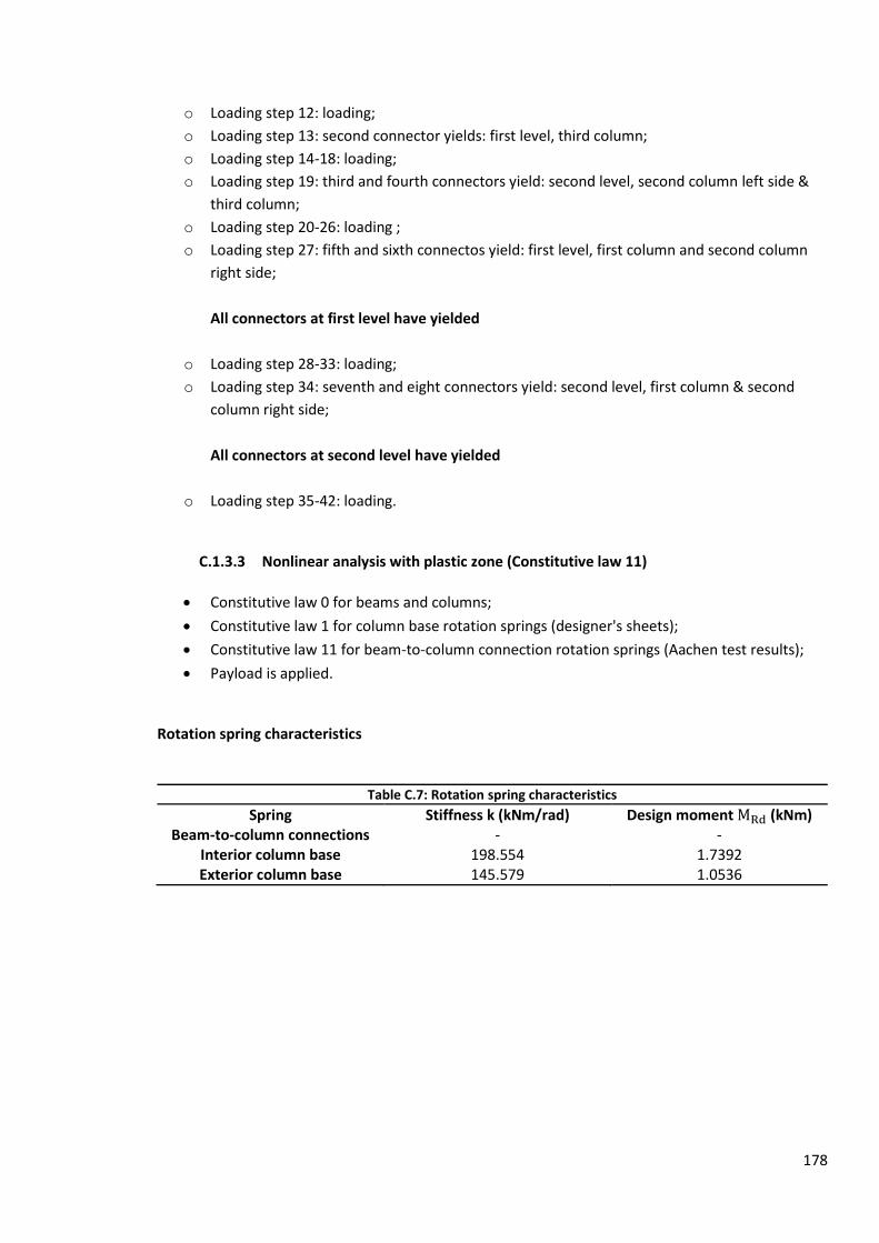
178

o Loading step 12: loading;

o Loading step 13: second connector yields: first level, third column;

o Loading step 14-18: loading;

o Loading step 19: third and fourth connectors yield: second level, second column left side &

third column;

o Loading step 20-26: loading ;

o Loading step 27: fifth and sixth connectos yield: first level, first column and second column

right side;

All connectors at first level have yielded

o Loading step 28-33: loading;

o Loading step 34: seventh and eight connectors yield: second level, first column & second

column right side;

All connectors at second level have yielded

o Loading step 35-42: loading.

C.1.3.3 Nonlinear analysis with plastic zone (Constitutive law 11)

Constitutive law 0 for beams and columns;

Constitutive law 1 for column base rotation springs (designer's sheets);

Constitutive law 11 for beam-to-column connection rotation springs (Aachen test results);

Payload is applied.

Rotation spring characteristics

Table C.7: Rotation spring characteristics

Spring Stiffness k (kNm/rad) Design moment (kNm) Beam-to-column connections - -

Interior column base 198.554 1.7392 Exterior column base 145.579 1.0536

179

Figure C.4: Beam-to-column rotation springs

Pushover curve

Figure C.5: Nonlinear analysis law 11

0

0,5

1

1,5

2

2,5

3

3,5

0 0,025 0,05 0,075 0,1 0,125 0,15

Mo

me

nt

(kN

m)

Rotation (rad)

Stepwise function fully loaded connectors

Stepwise function

-10

-9

-8

-7

-6

-5

-4

-3

-2

-1

0

1

2

0,00 0,25 0,50 0,75 1,00 1,25 1,50 1,75 2,00

Load

mu

ltip

lier

Displacement (m)

FL11

Pushover curve

180

Course of the test

o Loading step 1-8: Linear load-displacement curve;

o Loading step 9: Exterior column base yields: third column;

o Loading step 10: Exterior column base yields: third column;

o Loading step 11: Interior column base yields: second column;

All column bases have yielded

o Loading step 12-16: Loading, deterioration of connector stiffness;

o Loading step 17: First and second connectors yield: first level, second column left side and

third column;

o Loading step 18-20: Loading, deterioration of connector stiffness;

o Loading step 21: third and fourth connectors yield: first level, first column and second

column right side;

All first level connectors have yielded

o Loading step 22: fifth and sixth connectors yield: second level, second column left side and

third column;

o Loading step 23-29: Loading, deterioration of the connector stiffness;

o Loading step 30: seventh and eighth connectors yield: second level, first column and second

column right side;

All second level connectors have yielded

o Loading step 31-42: Loading, deterioration of the connector stiffness.

C.1.4 Calculation of failure rotations

For beam-to-column connectors, use is made of the moment-rotation curves adopted from

the tests conducted in Aachen (See Chapter 4);

For column bases, use is made of the SEISRACKS report[1] (page 51) (See Chapter 6);

Table C.8: Failure rotations

Connection (kNm) (kNm) (mrad) Beam-to-column 2.899 2.3192 147.6

Interior column base 1.7392 1.3914 53 Exterior column base 1.0536 0.8429 88

C.1.4.1 Determination of the end step (cut-off point)

Nonlinear analysis law 1

Cut off at step 24 (Interior column base reaches a rotation of 52.322 mrad).

181

Nonlinear analysis law 11

Cut off at step 17 (Interior column base reaches a rotation of 59.988 mrad).

C.1.5 Calculation of the failure parameter

C.1.5.1 Nonlinear analysis law 1 (design curve)

C.1.5.2 Nonlinear analysis law 11 (stepwise curve)

C.1.6 Calculation of the performance point

C.1.6.1 Nonlinear analysis law 1 (design curve)

Normalized horizontal forces

Transformation to an equivalent SDOF system

182

Determination of the idealized elastic-perfectly plastic force-displacement relationship

Determination of the period of the idealized equivalent SDOF system

Determination of the target displacement

Determination of the difference with

Second iteration

Corresponding shear force value calculated through linear interpolation:

183

Determination of the target displacement for the MDOF system

C.1.6.2 Nonlinear analysis law 11 (stepwise curve)

Normalized horizontal forces

Transformation to an equivalent SDOF system

Determination of the idealized elastic-perfectly plastic force-displacement relationship

Determination of the period of the idealized equivalent SDOF system

184

Determination of the target displacement

Determination of the difference with

Second iteration

Corresponding shear force value calculated through linear interpolation:

Determination of the target displacement for the MDOF system

185

C.1.7 Determination of the interstorey drift sensitivity factors

First storey

Second storey

Third storey

Fourth storey

186

C.1.8 Synthesis: monotonic analyses

All monotonic curves together in one graph;

Illustration of the failure load parameter and the performance point on the graph;

Curves cut off in respect with failure rotations.

Figure C.6: Synthesis

Legend

Linear: Linear elastic analysis;

FL0: Nonlinear analysis with Hooke's law;

FL1: Nonlinear analysis with elastic-perfectly plastic law (design curve of producer);

FL11: Nonlinear analysis with stepwise law for connectors (Aachen results) and elastic-

perfectly plastic law for column bases;

Lambda_P_1 : Calculated for design curve of the producer (FL1);

Lambda_P_11: Calculated for stepwise curve from Aachen results (FL11);

Perf_1: Performance point for FL1;

Perf_11: Performance point for FL11.

0

0,5

1

1,5

2

2,5

3

3,5

4

0,00 0,05 0,10 0,15 0,20 0,25 0,30

Load

mu

ltip

lier

Displacement (m)

Fully loaded case

FL0

FL1

FL11

Lambda_P_1

Linear

Lambda_P_11

Perf_1

Perf_11

187

C.2 Top loaded model

C.2.1 Modal Analysis

Table C.9: First mode

Mode Frequence (Hz) Period (s) Percentage of Collaborate Mass

(%)

1 0,460 2,172 100

C.2.2 Calculation of Horizontal forces

C.2.2.1 Input data

Table C.10: Input data

Parameter Value (m/s²) 1.4715 m/s²

1.0 Soil type C

Type of response spectrum 2 S 1.5

(s) 0.1 s (s) 0.25 s (s) 1.2 s

0.2 q 1.5

(kg) 2400 kg

0.8

1.0

C.2.2.2 Calculation of the base shear force

Calculation of the ordinate of the response spectrum

As :

Calculation of the total mass

188

Calculation of the seismic base shear force:

C.2.2.3 Calculation of the triangular distributed horizontal forces

Table C.11: Seismic action

Level z (m) m (kg) (kgm) F (kN) 1 1.9418 0 0 0 2 3.9418 0 0 0 3 5.9418 0 0 0 4 7.9418 2400 19060.32 0.5651

C.2.3 Monotonic analyses

C.2.3.1 Linear elastic analysis and nonlinear elastic analysis (Constitutive law 0)

Constitutive law 0 for all components;

No payload applied during linear elastic analysis;

Payload is applied during nonlinear elastic analysis.

Rotation spring characteristics

Table C.12: Rotation spring characteristics

Spring Stiffness k (kNm/rad) Design moment (kNm) Beam-to-column connections 112.448 -

Interior column base 79.756 - Exterior column base 39.880 -

Load-displacement curves

189

Figure C.7: Linear elastic analysis

Figure C.8: Nonlinear elastic analysis

0

2

4

6

8

10

12

0 0,05 0,1 0,15 0,2 0,25 0,3 0,35

Load

mu

ltip

lier

Displacement (m)

TL0 Linear

TL Linear

0

20

40

60

80

100

120

140

0,00 0,50 1,00 1,50 2,00 2,50 3,00 3,50 4,00

Load

mu

ltip

lier

Displacement (m)

TL0 Nonlinear

Pushover curve

190

C.2.3.2 Nonlinear analysis with plastic zone (Constitutive law 1)

Constitutive law 0 for beams and columns;

Constitutive law 1 for rotation springs (designer's sheets);

Payload is applied.

Rotation spring characteristics

Table C.13: Rotation spring characteristics

Spring Stiffness k (kNm/rad) Design moment (kNm) Beam-to-column connections 112.448 2.589

Interior column base 79.756 0.5483 Exterior column base 39.880 0.2744

Load-displacement curve

Figure C.9: Nonlinear analysis law 1

Course of the test

o Loading step 1-9: linearly increasing load-displacement curve;

o Loading step 10: all column bases yield;

All column bases have yielded

0

1

2

3

4

5

6

7

0,00 0,20 0,40 0,60 0,80 1,00 1,20 1,40

Load

mu

ltip

lier

Displacement (m)

TL1

Pushover curve

191

o Loading step 11-17: loading;

o Loading step 18: first and second connectors yield: first level, first and third column;

o Loading step 19: third and fourth connectors yield: first level, second column both sides;

All connectors at first level have yielded

o Loading step 20: loading;

o Loading step 21: fifth connector yields: fourth level, second column left side;

o Loading step 22: loading;

o Loading step 23: sixth and seventh connectors yield: second level, first column & third

column;

o Loading step 24: eighth and ninth connectors yield: second level, second column both sides;

All connectors at second level have yielded

o Loading step 25-28: loading;

o Loading step 29: tenth connector yields: fourth level, third column;

o Loading step 30: loading;

o Loading step 31: eleventh connector yields: third level, third column;

o Loading step 32: twelfth connector yields: third level, first column;

o Loading step 33: thirteenth and fourteenth connectors yield: third level, second column left

and right side;

All connectors at third level have yielded

o Loading step 34-39: loading ;

o Loading step 40: fifteenth connector yields: fourth level, first column;

o Loading step 41: sixteenth connector yields: fourth level, second column right side;

All connectors at fourth level have yielded

o loading step 42: loading.

C.2.3.3 Nonlinear analysis with plastic zone (Constitutive law 11)

Constitutive law 0 for beams and columns;

Constitutive law 1 for column base rotation springs (designer's sheets);

Constitutive law 11 for beam-to-column connection rotation springs (Aachen test results);

Payload is applied.

Rotation spring characteristics

Table C.14: Rotation spring characteristics

Spring Stiffness k (kNm/rad) Design moment (kNm) Beam-to-column connections - -

Interior column base 79.756 0.5483 Exterior column base 39.880 0.2744

192

Figure C.10: Beam-to-column rotation springs

Figure C.11: Beam-to-column rotation springs

0

0,5

1

1,5

2

2,5

3

3,5

0 0,025 0,05 0,075 0,1 0,125 0,15

Mo

me

nt

(kN

m)

Rotation (rad)

Stepwise function fully loaded connectors

Stepwise function

0

0,5

1

1,5

2

2,5

3

3,5

0 0,02 0,04 0,06 0,08 0,1 0,12

Mo

me

nt

(kN

m)

Rotation (rad)

Stepwise function unloaded connectors

Stepwise function

193

Pushover curve

Figure C.12: Nonlinear analysis law 11

Course of the test

o Loading step 1-11: Linear load-displacement curve;

o Loading step 12: All column bases yield;

All column bases have yielded

o Loading step 13-28: Loading, deterioration of the connector stiffness;

o Loading step 29: first and second connectors yield: first level, first and third column;

o Loading step 30: third and fourth connectors yield: first level, second column both sides;

All first level connectors have yielded

o Loading step 31-32: Loading, deterioration of the connector stiffness;

o Loading step 33: fifth and sixth connectors yield: second level, first and third column;

o Loading step 34: seventh and eighth connectors yield: second level, second column both

sides;

All second level connectors have yielded

o Loading step 35-36: Loading, deterioration of the connector stiffness;

o Loading step 37: ninth to thirteenth connectors yield: the whole third level and one at fourth

level, third column;

All third level connectors have yielded

0

1

2

3

4

5

6

7

8

0,00 0,20 0,40 0,60 0,80 1,00 1,20 1,40

Load

mu

ltip

lier

Displacement (m)

TL11

Pushover curve

194

o Loading step 38: fourteenth connector yields: fourth level, second column left side;

o Loading step 39-42: Loading, deterioration of the connector stiffness.

C.2.4 Calculation of failure rotations

For beam-to-column connectors, use is made of the moment-rotation curves adopted from

the tests conducted in Aachen (See Chapter 4);

For column bases, use is made of the SEISRACKS report[1] (page 51) (See Chapter 6);

Table C.15: Failure rotations

Connection (kNm) (kNm) (mrad) Beam-to-column fully loaded 2.899 2.3192 147.6 Beam-to-column top loaded 3.1558 2.5246 159

Interior column base 0.5483 0.4386 133 Exterior column base 0.2744 0.2195 160

C.2.4.1 Determination of the end step (cut-off point)

Nonlinear analysis law 1

Cut off at step 35 (Interior column base reaches a rotation of 125.75 mrad).

Nonlinear analysis law 11

Cut off at step 35 (Interior column base reaches a rotation of 133.42 mrad).

C.2.5 Calculation of the failure parameter

C.2.5.1 Nonlinear analysis law 1 (design curve)

C.2.5.2 Nonlinear analysis law 11 (stepwise curve)

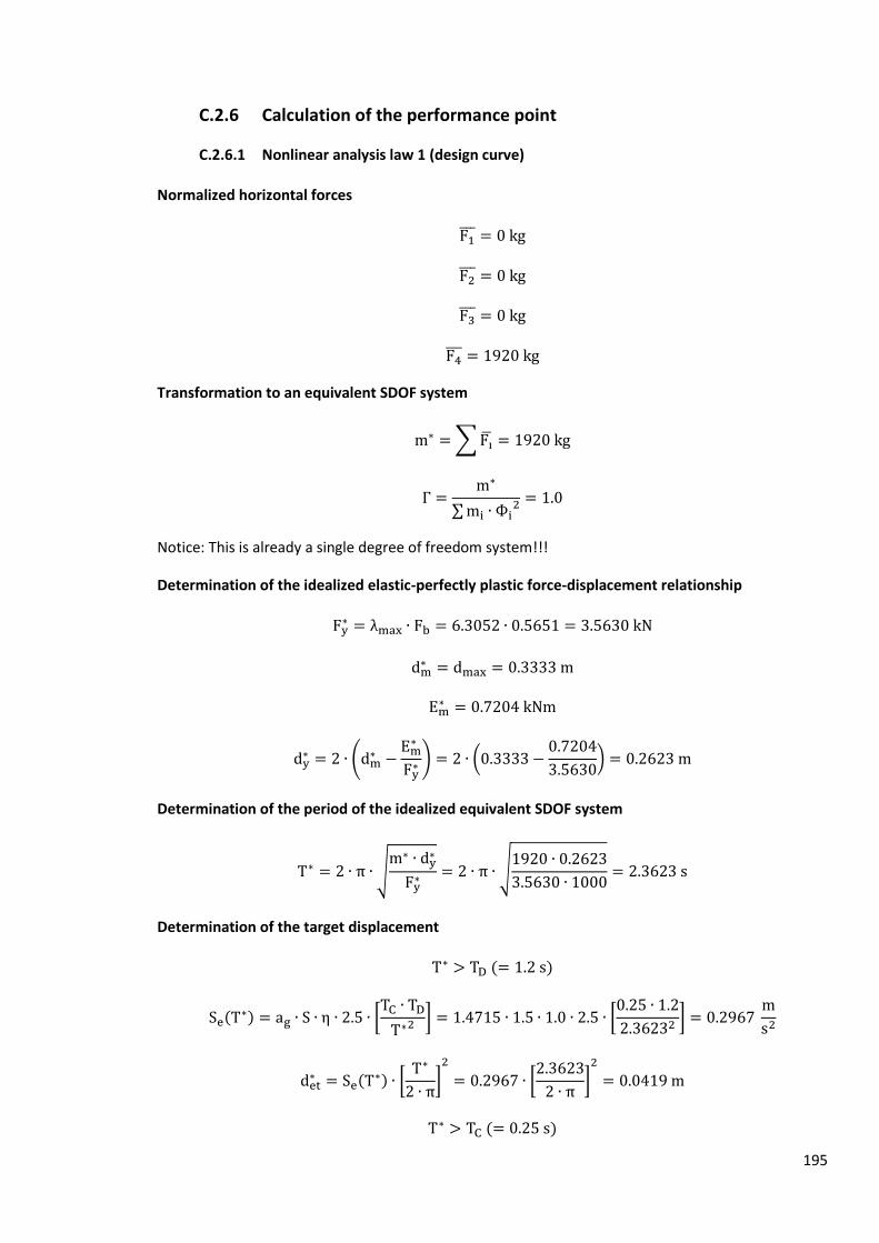
195

C.2.6 Calculation of the performance point

C.2.6.1 Nonlinear analysis law 1 (design curve)

Normalized horizontal forces

Transformation to an equivalent SDOF system

Notice: This is already a single degree of freedom system!!!

Determination of the idealized elastic-perfectly plastic force-displacement relationship

Determination of the period of the idealized equivalent SDOF system

Determination of the target displacement

196

Determination of the difference with

Second iteration

Corresponding shear force value calculated through linear interpolation:

Determination of the target displacement for the MDOF system

C.2.6.2 Nonlinear analysis law 11 (stepwise curve)

Normalized horizontal forces

197

Transformation to an equivalent SDOF system

Notice: This is already a single degree of freedom system!!!

Determination of the idealized elastic-perfectly plastic force-displacement relationship

Determination of the period of the idealized equivalent SDOF system

Determination of the target displacement

Determination of the difference with

Second iteration

198

Corresponding shear force value calculated through linear interpolation:

Determination of the target displacement for the MDOF system

C.2.7 Determination of the interstorey drift sensitivity factors

First storey

Second storey

199

As no difference exists in the values for the second, third and fourth storey, the latter two storeys

have the same -value.

Third storey

Fourth storey

C.2.8 Synthesis: monotonic analyses

All monotonic curves together in one graph;

Illustration of the failure load parameter and the performance point on the graph;

Curves cut off in respect with failure rotations.

200

Figure C.13: Synthesis

Legend

Linear: Linear elastic analysis;

TL0: Nonlinear analysis with Hooke's law;

TL1: Nonlinear analysis with elastic-perfectly plastic law (design curve of producer);

TL11: Nonlinear analysis with stepwise law for connectors (Aachen results) and elastic-

perfectly plastic law for column bases;

Lambda_P_1 : Calculated for design curve of the producer (TL1);

Lambda_P_11: Calculated for stepwise curve from Aachen results (TL11);

Perf_1: Performance point for TL1;

Perf_11: Performance point for TL11.

0

1

2

3

4

5

6

7

8

9

10

11

12

13

14

15

16

17

18

19

0,00 0,10 0,20 0,30 0,40 0,50 0,60 0,70

Load

mu

ltip

lier

Displacement (m)

Top loaded case

TL0

TL1

TL11

Lambda_P_1

Linear

Lambda_P_11

Perf_1

Perf_11

201

Annex D: Test report product D

For this product, the chosen system to be tested was the low seismicity system. The characteristics of

the beams and columns are the following:

Table D.1: Component characteristics

Component A [ ] I [ ] E [ ] Beam 665.4

Column 559.8

D.1 Fully loaded model

D.1.1 Modal Analysis

Table D.2: Modes

Mode Frequence (Hz) Period (s) Percentage of Collaborate Mass (%)

1 0.348 2.873 86.636

2 1.209 0.827 9.903

3 2.491 0.402 2.845

4 4.039 0.248 0.616

5 50.520 0.020 0.000

D.1.2 Calculation of Horizontal forces

D.1.2.1 Input data

Table D.3: Input data

Parameter Value (m/s²) 1.2

1.0 Soil type C

Type of response spectrum 2 S 1.5

(s) 0.1 (s) 0.25 (s) 1.2

0.2 q 2.0

(kg) 9600

0.8

1.0

202

D.1.2.2 Calculation of the base shear force

Calculation of the ordinate of the response spectrum

As :

So:

Calculation of the total mass

Calculation of the seismic base shear force

D.1.2.3 Calculation of the triangular distributed horizontal forces

Table D.4: Seismic action

Level z (m) m (kg) (kgm) F (kN) 1 1,9375 2400 4650 0,1808 2 3,9375 2400 9450 0,3675 3 5,9375 2400 14250 0,5541 4 7,9375 2400 19050 0,7408

D.1.3 Monotonic analyses

D.1.3.1 Linear elastic analysis and nonlinear elastic analysis (constitutive law 0)

Constitutive law 0 for all components;

No payload applied during linear elastic analysis;

Payload is applied during nonlinear elastic analysis.

203

Rotation spring characteristics

Table D.5: Rotation spring characteristics

Spring Stiffness k (kNm/rad) Design moment (kNm) Beam-to-column connections 112.448 -

Interior column base 156.715 - Exterior column base 83.023 -

Load-displacement curves

Figure D.1: Linear elastic analysis

Figure D.2: Nonlinear elastic analysis

0

0,5

1

1,5

2

2,5

3

3,5

4

4,5

0 0,05 0,1 0,15 0,2 0,25 0,3

Load

mu

ltip

lier

Displacement (m)

FL0 Linear

FL Linear

0

5

10

15

20

25

30

35

40

0,00 0,50 1,00 1,50 2,00 2,50 3,00 3,50

Load

mu

ltip

lier

Displacement (m)

FL0 Nonlinear

Pushover curve

204

D.1.3.2 Nonlinear analysis with plastic zone (Constitutive law 1)

Constitutive law 0 for beams and columns;

Constitutive law 1 for rotation springs (designer's sheets);

Payload is applied.

Rotation spring characteristics

Table D.6: Rotation spring characteristics

Spring Stiffness k (kNm/rad) Design moment (kNm) Beam-to-column connections 112.448 2.589

Interior column base 156.715 1.795 Exterior column base 83.023 0.993

Load-displacement curve

Figure D.3: Nonlinear analysis law 1

Course of the test

o Loading step 1-10: linearly increasing load-displacement curve;

o Loading step 11: exterior column bases yield;

o Loading step 12: interior column base yields;

All column bases have yielded

-5

-4

-3

-2

-1

0

1

2

0,00 0,10 0,20 0,30 0,40 0,50 0,60 0,70 0,80 0,90 1,00

Load

mu

ltip

lier

Displacement (m)

FL1

Pushover curve

205

o Loading step 13: first connector yields: first level, third column;

o Loading step 14: second connector yields: first level, second column, left side;

o Loading step 15-23: loading;

o Loading step 24: third connector yields: second level, third column;

o Loading step 25: fourth connector yields: second level, second column, left side;

o Loading step 26: loading;

o Loading step 27: fifth connector yields: first level, first column;

o Loading step 28: sixth connector yields: first level, second column, right side;

All connectors at first level have yielded

o Loading step 29-33: loading;

o Loading step 34: seventh connector yields: second level, first column;

o Loading step 35: eighth connector yields: second level, second column, right side;

All connectors at second level have yielded

o Loading step 36-42: Loading.

D.1.3.3 Nonlinear analysis with plastic zone (Constitutive law 11)

Constitutive law 0 for beams and columns;

Constitutive law 1 for column base rotation springs (designer's sheets);

Constitutive law 11 for beam-to-column connection rotation springs (Aachen test results);

Payload is applied.

Rotation spring characteristics

Table D.7: Rotation spring characteristics

Spring Stiffness k (kNm/rad) Design moment (kNm) Beam-to-column connections - -

Interior column base 156.715 1.795 Exterior column base 83.023 0.993

206

Figure D.4: Beam-to-column rotation springs

Pushover curve

Figure D.5: Nonlinear analysis law 11

0

0,5

1

1,5

2

2,5

3

3,5

0 0,02 0,04 0,06 0,08 0,1 0,12

Mo

me

nt

(kN

m)

Rotation (rad)

Stepwise function fully loaded connectors

Stepwise function

-5

-4

-3

-2

-1

0

1

2

0,00 0,10 0,20 0,30 0,40 0,50 0,60 0,70 0,80 0,90 1,00 1,10

Load

mu

ltip

lier

Displacement (m)

FL11

Pushover curve

207

Course of the test

o Loading step 1-12 : linearly increasing load-displacement curve;

o Loading step 13: exterior column base yields: third column;

o Loading step 14: exterior and interior column bases yield;

All column bases have yielded

o Loading step 15-27: loading, deterioration of connector stiffnesses;

o Loading step 28: first and second connectors fail: first level, second column left and third

column;

o Loading step 29-30: loading, derterioration of connector stiffnesses;

o Loading step 31: third and fourth connectors fail: first level, second column right and first

column;

All first level connectors have yielded

o Loading step 32-33: loading, derterioration of connector stiffnesses;

o Loading step 34: fifth connector fails: second level, third column;

o Loading step 35: sixth connector fails: second level, second column left side;

o Loading step 36-38: loading, derterioration of connector stiffnesses;

o Loading step 39: seventh connector fails: second level, first column;

o Loading step 40: eigth connector fails: second level, second column right side;

All second level connectors have yielded

o Loading step 41: loading, derterioration of connector stiffnesses;

o Loading step 42: loading, derterioration of connector stiffnesses.

D.1.4 Calculation of failure rotations

For beam-to-column connectors, use is made of the moment-rotation curves adopted from

the tests conducted in Aachen (See Chapter 4);

For column bases, use is made of the SEISRACKS report[1] (page 51) (See Chapter 6);

Table D.8: Failure rotations

Connection (kNm) (kNm) (mrad) Beam-to-column 3.330 2.664 132

Interior column base 1.7949 1.4359 51 Exterior column base 0.9934 0.7947 87

D.1.4.1 Determination of the end step (cut-off point)

Nonlinear analysis law 1

Cut off at step 26 (Interior column base reaches a rotation of 51.667 mrad).

208

Nonlinear analysis law 11

Cut off at step 27 (Interior column base reaches a rotation of 52.733 mrad).

D.1.5 Calculation of the failure parameter

D.1.5.1 Nonlinear analysis law 1 (design curve)

D.1.5.2 Nonlinear analysis law 11 (stepwise curve)

D.1.6 Calculation of the performance point

D.1.6.1 Nonlinear analysis law 1 (design curve)

Normalized horizontal forces

Transformation to an equivalent SDOF system

209

Determination of the idealized elastic-perfectly plastic force-displacement relationship

Determination of the period of the idealized equivalent SDOF system

Determination of the target displacement

Determination of the difference with

Second iteration

Corresponding shear force value calculated through linear interpolation:

210

Determination of the target displacement for the MDOF system

D.1.6.2 Nonlinear analysis law 11 (stepwise curve)

Normalized horizontal forces

Transformation to an equivalent SDOF system

Determination of the idealized elastic-perfectly plastic force-displacement relationship

Determination of the period of the idealized equivalent SDOF system

211

Determination of the target displacement

Determination of the difference with

Second iteration

Corresponding shear force value calculated through linear interpolation:

Determination of the target displacement for the MDOF system

212

D.1.7 Determination of the interstorey drift sensitivity factors

First storey

Second storey

Third storey

Fourth storey

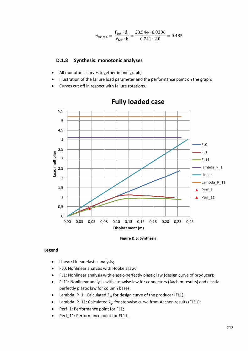
213

D.1.8 Synthesis: monotonic analyses

All monotonic curves together in one graph;

Illustration of the failure load parameter and the performance point on the graph;

Curves cut off in respect with failure rotations.

Figure D.6: Synthesis

Legend

Linear: Linear elastic analysis;

FL0: Nonlinear analysis with Hooke's law;

FL1: Nonlinear analysis with elastic-perfectly plastic law (design curve of producer);

FL11: Nonlinear analysis with stepwise law for connectors (Aachen results) and elastic-

perfectly plastic law for column bases;

Lambda_P_1 : Calculated for design curve of the producer (FL1);

Lambda_P_11: Calculated for stepwise curve from Aachen results (FL11);

Perf_1: Performance point for FL1;

Perf_11: Performance point for FL11.

0

0,5

1

1,5

2

2,5

3

3,5

4

4,5

5

5,5

0,00 0,03 0,05 0,08 0,10 0,13 0,15 0,18 0,20 0,23 0,25

Load

mu

ltip

lier

Displacement (m)

Fully loaded case

FL0

FL1

FL11

lambda_P_1

Linear

Lambda_P_11

Perf_1

Perf_11

214

D.2 Top loaded model

D.2.1 Modal Analysis

Table D.9: First mode

Mode Frequence (Hz) Period (s) Percentage of Collaborate Mass

(%)

1 0.459 2.176 100

D.2.2 Calculation of Horizontal forces

D.2.2.1 Input data

Table D.10: Input data

Parameter Value (m/s²) 1.2 m/s²

1.0 Soil type C

Type of response spectrum 2 S 1.5

(s) 0.1 s (s) 0.25 s (s) 1.2 s

0.2 q 2.0

(kg) 2400 kg

0.8

1.0

D.2.2.2 Calculation of the base shear force

Calculation of the ordinate of the response spectrum

As :

Calculation of the total mass

215

Calculation of the seismic base shear force:

D.2.2.3 Calculation of the triangular distributed horizontal forces:

Table D.11: Seismic action

Level z (m) m (kg) (kgm) F (kN) 1 1,9375 0 0 0 2 3,9375 0 0 0 3 5,9375 0 0 0 4 7,9375 2400 19050 0.4608

D.2.3 Monotonic analyses

D.2.3.1 Linear elastic analysis and nonlinear elastic analysis (Constitutive law 0)

Constitutive law 0 for all components;

No payload applied during linear elastic analysis;

Payload is applied during nonlinear elastic analysis.

Rotation spring characteristics

Table D.12: Rotation spring characteristics

Spring Stiffness k (kNm/rad) Design moment (kNm) Beam-to-column connections 112.448 -

Interior column base 41.240 - Exterior column base 20.620 -

Load-displacement curves

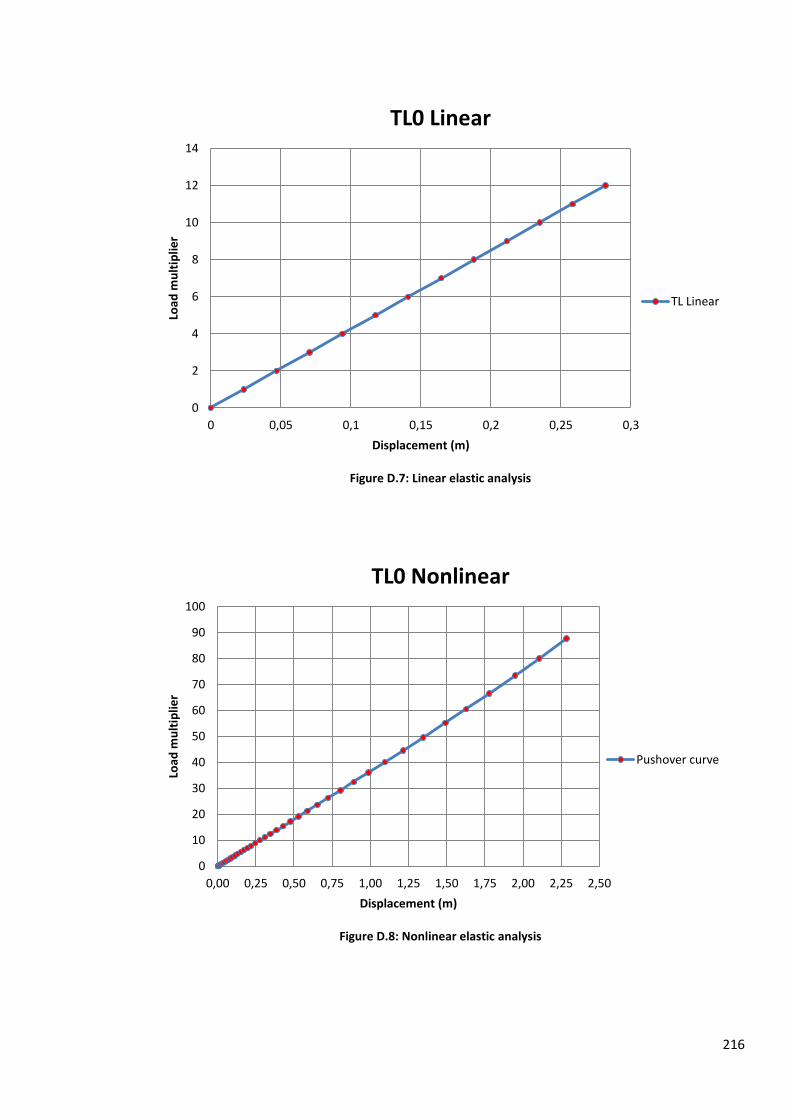
216

Figure D.7: Linear elastic analysis

Figure D.8: Nonlinear elastic analysis

0

2

4

6

8

10

12

14

0 0,05 0,1 0,15 0,2 0,25 0,3

Load

mu

ltip

lier

Displacement (m)

TL0 Linear

TL Linear

0

10

20

30

40

50

60

70

80

90

100

0,00 0,25 0,50 0,75 1,00 1,25 1,50 1,75 2,00 2,25 2,50

Load

mu

ltip

lier

Displacement (m)

TL0 Nonlinear

Pushover curve

217

D.2.3.2 Nonlinear analysis with plastic zone (Constitutive law 1)

Constitutive law 0 for beams and columns;

Constitutive law 1 for rotation springs (designer's sheets);

Payload is applied.

Rotation spring characteristics

Table D.13: Rotation spring characteristics

Spring Stiffness k (kNm/rad) Design moment (kNm) Beam-to-column connections 112.448 2.589

Interior column base 41.240 0.591 Exterior column base 20.620 0.392

Load-displacement curve

Figure D.9: Nonlinear analysis law 1

Course of the test

o Loading step 1-12: linearly increasing load-displacement curve;

o Loading step 13: interior column base yields;

o Loading step 14: loading;

o Loading step 15: exterior column bases yield;

All column bases have yielded

0

1

2

3

4

5

6

7

8

9

0,00 0,20 0,40 0,60 0,80 1,00 1,20 1,40

Load

mu

ltip

lier

Displacement (m)

TL1

Pushover curve

218

o Loading step 16-19:loading;

o Loading step 20: first and second connectors yield: first level, first and third column;

o Loading step 21: loading;

o Loading step 22: third and fourth connectors yield: first level, second column left and right;

All connectors at first level have yielded

o Loading step 23: loading;

o Loading step 24: fifth and sixth connectors yield: second level, first and third column;

o Loading step 25: seventh and eight connectors yield: second level, second column left and

right;

All connectors at second level have yielded

o Loading step 26-30: loading;

o Loading step 31: ninth connector yields: third level, third column;

o Loading step 32: tenth connector yields: third level, first column;

o Loading step 33: eleventh and twelfth connectors yield: third level, second column left and

right;

All connectors at third level have yielded

o Loading step 34: thirteenth and fourteenth connectors yield: fourth level, second column left

side and third column;

o Loading step 35-39: loading;

o Loading step 40: fifteenth connector yields: fourth level, first column;

o Loading step 41: sixteenth connector yields: fourth level, second column right side;

All connectors at fourth level have yielded

o loading step 42: loading.

D.2.3.3 Nonlinear analysis with plastic zone (Constitutive law 11)

Constitutive law 0 for beams and columns;

Constitutive law 1 for column base rotation springs (designer's sheets);

Constitutive law 11 for beam-to-column connection rotation springs (Aachen test results);

Payload is applied.

Rotation spring characteristics

Table D.14: Rotation spring characteristics

Spring Stiffness k (kNm/rad) Design moment (kNm) Beam-to-column connections - -

Interior column base 41.240 0.591 Exterior column base 20.620 0.392

219

Figure D.10: Beam-to-column rotation springs

Figure D.11: Beam-to-column rotation springs

0

0,5

1

1,5

2

2,5

3

3,5

0 0,02 0,04 0,06 0,08 0,1 0,12

Mo

me

nt

(kN

m)

Rotation (rad)

Stepwise function fully loaded connectors

Stepwise function

0

0,5

1

1,5

2

2,5

3

3,5

0 0,02 0,04 0,06 0,08 0,1 0,12

Mo

me

nt

(kN

m)

Rotation (rad)

Stepwise function unloaded connectors

Stepwise function

220

Pushover curve

Figure D.12: Nonlinear analysis law 11

Course of the test

o Loading step 1-14: Linear load-displacement curve;

o Loading step 15: Interior column base yields;

o Loading step 16: loading, deterioration of the connector stiffness;

o Loading step 17: Exterior column bases yield;

All column bases have yielded

o Loading step 18-28: loading, deterioration of the connector stiffness;

o Loading step 29: first and second connectors yield: first level, first and third column;

o Loading step 30: third and fourth connectors yield: first level, second column both sides;

All first level connectors have yielded

o Loading step 31-37: loading, deterioration of the connector stiffness;

o Loading step 38: fifth and sixth connectors yield: second level, first and third column;

o Loading step 39: seventh and eighth connectors yield: second level, second column both

sides;

All second level connectors have yielded

o Loading step 40-42: loading, deterioration of the connector stiffness.

0

1

2

3

4

5

6

7

8

9

0,00 0,10 0,20 0,30 0,40 0,50 0,60 0,70 0,80

Load

mu

ltip

lier

Displacement (m)

TL11

Pushover curve

221

D.2.4 Calculation of failure rotations

For beam-to-column connectors, use is made of the moment-rotation curves adopted from

the tests conducted in Aachen (See Chapter 4);

For column bases, use is made of the SEISRACKS report[1] (page 51) (See Chapter 6);

Table D.15: Failure rotations

Connection (kNm) (kNm) (mrad) Beam-to-column fully loaded 3.330 2.664 132 Beam-to-column top loaded 3.330 2.664 121.9

Interior column base 0.5910 0.4728 133 Exterior column base 0.3924 0.3139 160

D.2.4.1 Determination of the end step (cut-off point)

Nonlinear analysis law 1

Cut off at step 36 (Interior column base reaches a rotation of 132.43 mrad).

Nonlinear analysis law 11

Cut off at step 42 (Interior column base reaches a rotation of 133.49 mrad).

D.2.5 Calculation of the failure parameter

D.2.5.1 Nonlinear analysis law 1 (design curve)

D.2.5.2 Nonlinear analysis law 11 (stepwise curve)

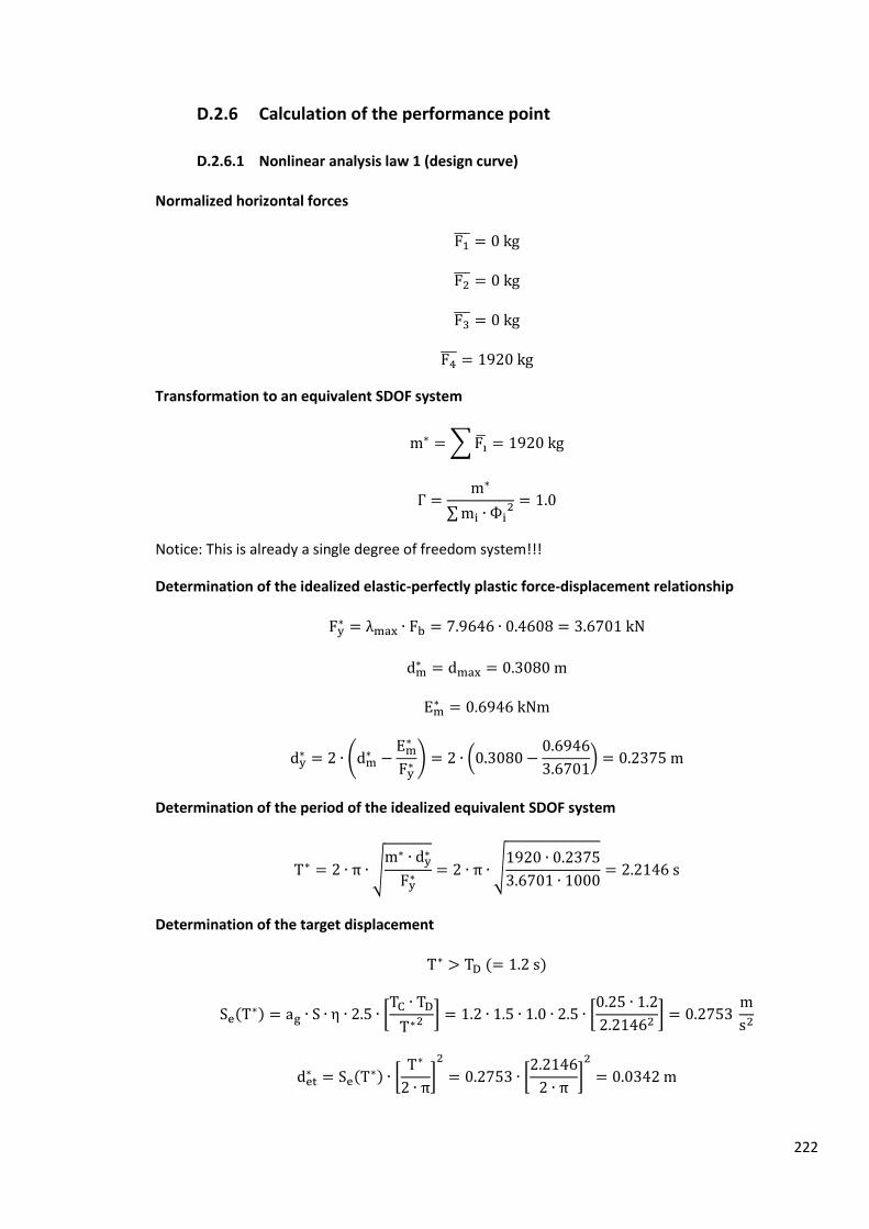
222

D.2.6 Calculation of the performance point

D.2.6.1 Nonlinear analysis law 1 (design curve)

Normalized horizontal forces

Transformation to an equivalent SDOF system

Notice: This is already a single degree of freedom system!!!

Determination of the idealized elastic-perfectly plastic force-displacement relationship

Determination of the period of the idealized equivalent SDOF system

Determination of the target displacement

223

Determination of the difference with

Second iteration

Corresponding shear force value calculated through linear interpolation:

Determination of the target displacement for the MDOF system

D.2.6.2 Nonlinear analysis law 11 (stepwise curve)

Normalized horizontal forces

224

Transformation to an equivalent SDOF system

Notice: This is already a single degree of freedom system!!!

Determination of the idealized elastic-perfectly plastic force-displacement relationship

Determination of the period of the idealized equivalent SDOF system

Determination of the target displacement

Determination of the difference with

Second iteration

225

Corresponding shear force value calculated through linear interpolation:

Determination of the target displacement for the MDOF system

D.2.7 Determination of the interstorey drift sensitivity factors

First storey

Second storey

226

As no difference exists in the values for the second, third and fourth storey, the latter two storeys

have the same -value.

Third storey

Fourth storey

D.2.8 Synthesis: monotonic analyses

All monotonic curves together in one graph;

Illustration of the failure load parameter and the performance point on the graph;

Curves cut off in respect with failure rotations.

227

Figure D.13: Synthesis

Legend

Linear: Linear elastic analysis;

TL0: Nonlinear analysis with Hooke's law;

TL1: Nonlinear analysis with elastic-perfectly plastic law (design curve of producer);

TL11: Nonlinear analysis with stepwise law for connectors (Aachen results) and elastic-

perfectly plastic law for column bases;

Lambda_P_1 : Calculated for design curve of the producer (TL1);

Lambda_P_11: Calculated for stepwise curve from Aachen results (TL11);

Perf_1: Performance point for TL1;

Perf_11: Performance point for TL11.

0

5

10

15

20

25

0,00 0,10 0,20 0,30 0,40 0,50 0,60 0,70

Load

mu

ltip

lier

Displacement (m)

Top loaded case

TL0

TL1

TL11

Lambda_P_1

Linear

Lambda_P_11

Perf_1

Perf_11

228

References

[1] Ing. I. Rosin, Geom. G. Coracina, Prof. L. Calado, Prof. J. Proença, Prof. P. Carydis, Prof. H.

Mouzakis, Prof. C. Castiglioni, Dr. J.C. Brescianini, Prof. A. Plumier, Prof. H. Degée, Dr. P. Negro,

Dr. F. Molina. "Storage Racks in Seismic Areas, Final Report." Research Fund for Coal and Steel,

2007.

[2] FEM 10.2.08. "Recommendations for the Design of Static Steel Pallet Racks under Seismic

Conditions." European Federation of Materials Handling, 2010.

[3] EN 1998 - Eurocode 8. "Design of structures for earthquake resistance." European Committee

for Standardisation, Brussels, 2005.

[4] "International building code 2003." International Code Council, Falls Church, Virginia, 2003.

[5] NFPA 5000. "NFPA building construction and safety code." National Fire Protection

Association, Quincy, Massachusetts, 2003.

[6] RMI. "Specification for the Design, Testing and Utilization of Industrial Steel Storage Racks."

Rack Manufacturers Institute, 2012.

[7] CSA A344. "Standards for the Design and Construction of Steel Storage Racks." Canadian

Standards Association, 2010.

[8] As 4084. "Steel Storage Racking." Standards Australia, Sydney, 1993.

[9] AS 4100. "Steel Structures." Standards Australia, Sydney, 1998.

[10] RMI. "Specification for the Design, Testing and Utilization of Industrial Steel Storage Racks."

Rack Manufacturers Institute, 2008.

[11] EN 15512. "Steel Static Storage Systems - Adjustable Pallet Racking - Principles for Structural

Design." European Committee for Standardisation, Brussels, 2009.

[12] As 4084. "Steel Storage Racking." Standards Australia, Sydney, 2012.

[13] "FineLg, V9.3 ." Software package, Department ArGEnCo - University of Liège and Engineering

Office Greisch, Liège.

[14] Pr FEM 10.2.08. "Recommendations for the Design of Static Steel Pallet Racks under Seismic

Conditions." European Federation of Materials Handling, 2008.

[15] "Reighley Pallet Rack Systems." Web page, January 2013.

(http://www.reighleyresources.com/PalletRackSystems)

229

[16] "Stow Pallet Racking." Web page, January 2013.

(http://www.southward.co.nz/page/13-pallet-racking)

[17] A. Filiatrault, A. Wanitkorkul and P. Higgins. "Experimental Stiffness and Seismic Response of

Pallet-Type Steel Storage Rack Connectors." ASCE Practice Periodical on Structural Design and

Construction, no. 11, pp. 161-170, 2006.

[18] Chen C.K., Scholl R.E., Blume J.A. "Seismic study of industrial storage racks." Rep. Prepared for

the National Science Foundation and for the Rack Manufacturers Institute and Automated

Storage and Retrieval Systems (Sections of the Material Handling Institute), URS/John A. Blume

& Associates, San Francisco, 1980.

[19] "SAP 2000." Software package, Computers and Structures Inc., Berkeley, California.

[20] Benoit P. Gilbert, Kim J. R. Rasmussen. "Determination of the Base Plate Stiffness and Strength

of Steel Storage Racks." Journal of Constructional Steel Research, no. 67, pp. 1031-1041, 2011.

[21] Kosteski N., Packer J.A. "Welded Tee-to-Hss Connections." Journal of Structural Engineering,

no. 129, pp. 151-159, 2003.

[22] Yura J.A., Zettlemoyer N., Edwards I.F. "Ultimate Capacity Equations for Tubular Joints." 12th

annual offshore technology conference, 1980.

[23] Sarawit A.T. "Cold-Formed Steel Frame and Beam-Column Design." School of Civil and

Environmental Engineering, Cornell University, 2003.

[24] Godley M.H.R., Beale R.G., Feng X. "Rotational Stiffness of Semi-Regid Baseplates." Yu W.W.,

LaBoule R.A. (Eds.), 14th international specialty conference on cold-formed steel structures,

pp. 323-325, 1998.

[25] "Strand 7." Software package, Strand7 Pty Ltd., Sydney

[26] Degée H. "New European Recommendations for the Design of Static Steel Pallet Racks in

Seismic Conditions - the Fem 10.2.08 Code of Practice." 6th International Conference on Thin

Walled Structures, 2011.

[27] Feldmann M., Heinemeyer C., Hofmeister B. "SEISRACKS 2: Tests on Seismic Performance of

Racks, Beam End Connectors in Down Aisle Direction." Institut und Lehrstuhl für Stahlbau und

Leichtmetallbau, Aachen, 2013.

[28] "ECCS." Web page, February 2013.

(http://www.steelconstruct.com)

[29] Feldmann M., Heinemeyer C., Hofmeister B. "SEISRACKS 2: Tests on Seismic Performance of

Racks, Column Base Tests." Institut und Lehrstuhl für Stahlbau und Leichtmetallbau, Aachen,

2013.

230

[30] "FineLg, User's Manual, V9.3" Software package, Department ArGEnCo - University of Liège

and Engineering Office Greisch, Liège.

[31] Prof. Hervé Degée. "Seismic Design." Course, Faculty of Engineering and Architecture, Ghent

University, 2012-2013.

[32] EN 1990 - Eurocode 0. "Basis of structural design." European Committee for Standardisation,

Brussels, 2002.

[33] Prof. Dr. Ir. Rudy Van Impe., Prof. Dr. Ir. Luc Taerwe. "Nonlinear and Plastic Methods of

Structural Analysis." Course, Faculty of Engineering and Architecture, Ghent University, 2012-

2013.