Experimental comparison of classical pid and model-free control

HAL Id: inria-00563941https://hal.inria.fr/inria-00563941

Submitted on 7 Feb 2011

HAL is a multi-disciplinary open accessarchive for the deposit and dissemination of sci-entific research documents, whether they are pub-lished or not. The documents may come fromteaching and research institutions in France orabroad, or from public or private research centers.

L’archive ouverte pluridisciplinaire HAL, estdestinée au dépôt et à la diffusion de documentsscientifiques de niveau recherche, publiés ou non,émanant des établissements d’enseignement et derecherche français ou étrangers, des laboratoirespublics ou privés.

Experimental comparison of classical pid and model-freecontrol: position control of a shape memory alloy active

springPierre-Antoine Gédouin, Emmanuel Delaleau, Jean-Matthieu Bourgeot,

Cédric Join, Shabnam Arbab-Chirani, Sylvain Calloch

To cite this version:Pierre-Antoine Gédouin, Emmanuel Delaleau, Jean-Matthieu Bourgeot, Cédric Join, Shabnam Arbab-Chirani, et al.. Experimental comparison of classical pid and model-free control: position control of ashape memory alloy active spring. Control Engineering Practice, Elsevier, 2011, 19 (5), pp.433-441.<10.1016/j.conengprac.2011.01.005>. <inria-00563941>

https://hal.inria.fr/inria-00563941

https://hal.archives-ouvertes.fr

Experimental comparison of classical pid and

model-free control: position control of a shape memory

alloy active spring✩

Pierre-Antoine Gedouina,1, Emmanuel Delaleau∗,a, Jean-MatthieuBourgeota, Cedric Joinb,c, Shabnam Arbab Chirania, Sylvain Callochd

aEcole Nationale d’Ingenieurs de Brest, LBMS (Laboratoire Brestois de Mecanique et desSystemes – EA 4325), Technopole Brest-Iroise, CS 73862, 29238 Brest Cedex 3, France.

http://www.enib.fr

Universite europeenne de Bretagne, FrancebCentre de recherche en automatique de Nancy, UMR CNRS 7039, Universite Henry

Poincare-Nancy I, Faculte des sciences et techniques, BP 239, 54 506 Vandœuvre, FrancecEquipe-projet ALIEN, Institut national de la recherche en informatique et automatique.

http://www.math-info.univ-paris5.fr/ mboup/ALIENdEcole Nationale Superieure d’Ingenieurs d’Etudes et Techniques d’Armement, LBMS(Laboratoire Brestois de Mecanique et des Systemes, EA 4325), 2 rue Francois Verny,

29 806 Brest cedex 9, France. http://www.ensieta.fr

Universite europeenne de Bretagne, France

Abstract

Shape memory alloys (sma) are more and more integrated in engineering

applications. These materials with their shape memory effect permit to sim-

✩This work was supported in part by the Agence nationale de la recherche (France)— Project “Tools for modelling, design and control of smart structural systems based onshape memory alloy (MAFESMA)”, in part by Brest metropole oceane, in part by Conseilgeneneral du Finistere.

∗Corresponding author. Tel.: +33 298 056 650; Fax: +33 298 056 653.Email addresses: [email protected] (Pierre-Antoine Gedouin), [email protected]

(Emmanuel Delaleau), [email protected] (Jean-Matthieu Bourgeot),[email protected] (Cedric Join), [email protected] (Shabnam ArbabChirani), [email protected] (Sylvain Calloch)

1P.-A. Gedouin is partially supported by Brest metropole oceane.

Preprint submitted to Control Engineering Practice April 1, 2010

plify mechanisms and to reduce the size of actuators. sma parts can easily be

activated by Joule effect but their modelling and consequently their control

remains difficult, it is principally due to their hysteretic thermomechanical

behaviour. Most of successful control strategy applied to sma actuator are

not often suitable for industrial applications: they are particularly heavy and

use the Preisach model or neural networks to model the hysteretic behaviour

of these material; this kind of models are difficult to identify and to use in real

time. That is why this paper deals with an application of the new framework

of model-free control (mfc) to a sma spring based actuator. This control

strategy is based on new results on fast derivatives estimation of noisy sig-

nals, its main advantages are: its simplicity and its robustness. Experimental

results and comparisons with pi control are exposed that demonstrate the

efficiency of this new control strategy.

Key words: Nonlinear control, Model-free control, Shape memory alloy,

Derivative estimation, Nonphysical modelling.

1. Introduction

Shape memory alloys (sma) actuators offer the possibility to recover a

known shape after a thermomechanical cycle. This property, known as the

“shape memory effect”, is due to the transition between the two crystallo-

2

graphic phases in their composition (i.e., the transition between martensite

and austenite). This variation of shape, controlled by temperature variation,

can be used in the development of actuators (see e.g., Janker et al., 2008;

Peirs et al., 2002; Kohl et al., 2002). sma can easily be heated by Joule effect,

but their control is not completely solved and it is principally due to their

hysteretic behaviour (see Patoor et al., 1994). Another difficulty is that the

characteristics of the material are time-varying, especially during cyclic load-

ings. Phases kinetic transformations and 3-dimensional models are proposed

in Sittner et al. (2000), Arbab Chirani et al. (2003) and Bouvet et al. (2004).

These complex models can render very subtle properties of sma, but often

need to compute a finite element code, what is not suitable for real time con-

trol. On the opposite side, Robotics research has been done on sma actuator

by using simpler model and classical control method. A lot of control strate-

gies have been applied to sma actuators, classical pid loop are used in Calin

et al. (1997), Shameli et al. (2005) and Da Silva (2007). A feedforward path

is added in Majima et al. (2001) and Ahn and Kha (2007); the feedforward

command is obtain by using a Preisach model for the hysteretic effect. In

Dutta et al. (2005) feedforward scheme is also used but the hysteretic be-

haviour is described by a Duhem differential hysteresis model. In Song et al.

3

(2003) and Romano and Aoun Tannuri (2009) a feedforward loop is com-

bined with sliding mode control to obtain robustness, the feedforward path

is respectively given by neural network and by a physical model. In Jayender

et al. (2005), the gains of a PI controller have been tuned by H∞ loop shap-

ing considering a physical model linearised around some operating points.

Passivity property of the system is used in Madill and Wang (1998) to prove

stability of a proposed proportional law. Nonlinear control techniques based

on the Lie algebra are also used in Benzaoui et al. (1999). Even if the model

is good enough, using a dynamic model for computing the control law implies

the identification of the model parameters. As already mentioned, the model

parameters of sma vary during cycling, then a classical model-based con-

trol is ineffective or particularly complex. We report our experience, where

industrial partners still explain that in order to realise the process control,

the part of process modelling represents 90% of project global time and re-

quires a true know-how in control and about the process to-be controlled.

Indeed, the choice of the physical model structure, the identification of the

model parameters, the experimental validation of model are never simple.

pid controllers are often tuned with a simple (linear) non physical model

(an extensive literature about this subject is available see e.g., Astrom and

4

Hagglund, 2005, 1995; Visioli, 2005; Ang et al., 2005; Panagopoulos et al.,

2002; Khodabakhshian and Edrisi, 2008; Gyongy and Clarke, 2006; Tavakoli

et al., 2006), that is why pid control is often preferred to physical model-

based control in the industry. However, pid controllers could render poor

results when a process has a large operating domain. So, how is it possible

to efficiently control a complex process:

• without complex physical model ?

• with easy-to-use and theoretically understandable controllers ?

In this paper, a solution2 to this difficult problem is proposed. The propo-

sition is based on some new results in the framework of “model-free control”

(see Fliess and Join, 2009; Fliess et al., 2006; Join et al., 2006). The approach

uses derivative estimations (see Mboup et al., 2008, 2007; Fliess et al., 2008)

which provides good results even if the measured signals are corrupted by

noise. Thus a non-physical model valid a very short part of time is estimated

and permits classical control design.

The present work constitutes an extension of two previous articles: In Gedouin

et al. (2008), the advantages of model-free control of sma has been high-

2See, e.g., Han (2009) for another approach.

5

lighted by simulations while preliminary experimental results have been pre-

sented in Gedouin et al. (2009).

The paper is organised as follows: The next Section gives an introduc-

tion to the new “model-free control” and explains the design of a control law

within this framework; Sec. 3 develops the model-free control of a shape mem-

ory alloys actuator and gives experimental results. Sec. 4 develops a simple

improvement of the model-free controller and the PI controller; this modifi-

cation results in position dependent gain of the control; this gain is obtain

by steady state identification of an input-output nonphysical process model;

experimental and robustness results of the modified controller are presented

in great details. Sec. 5 concludes the paper and raises some perspectives.

2. Model-free control

Model-free control is a very recent approach to nonlinear control that

has been introduced in Fliess et al. (2006), (see Fliess and Join, 2009, for a

thorough presentation). A first industrial and application is reported in Join

et al. (2008).

6

2.1. Derivatives of noisy signals

We recall basics of derivative estimation. Interested reader might refer

to Mboup et al. (2008) for a complete presentation. The method presented

here, consists in designing FIR filters resolving a classical polynomial approx-

imation of the signal. The polynomial approximation is obtained by algebraic

manipulation of signals in the operational domain. We consider a signal y

that is available through a measurement ym corrupted by some additive noise

, i.e. ym = y + . The objective is to estimate time derivatives of signal

y(t), up to a finite order, from its measurement ym.

The Taylor expansion of y around 0 reads:

y(t) =∞∑

n=0

y(n)(0)

n!tn (1)

Approximate y(t) in the interval [0, T ], T > 0, by the polynomial yN(τ) =

∑Nn=0 y(n)(0) τn

n!of degree N . The operational3 analogue (see Mikusinski,

1983) YN(s) of yN(τ) is given by:

YN(s) =y(0)

s+

y(0)

s2+ · · ·+

y(N)(0)

sN+1(2)

It is possible to isolate each coefficient y(i)(0) appearing in the previous

3Reader not familiar with operational calculus can just think in terms of Laplace trans-

form to understand the development of the derivatives estimators.

7

expression by applying a convenient operator to YN(s) (see Mboup et al.,

2008, for details4). Indeed:

∀i = 0, . . . , N,y(i)(0)

s2N+1=

(−1)i

i!(N − i)!·

1

sN+1·

di

dsi·1

s·

dN−i

dsN−i

(sN+1YN(s)

)(3)

The two following formulas of operational calcul (Mikusinski (1983)) are very

useful:

• the operator 1sα corresponds to the function t 7→ tα−1

(α−1)!

• the operator dds

corresponds to the multiplication in the time domain

by −t

Moreover, the Cauchy formulae to transform a multiple integral in a simple

one:

∫ T

0

∫ τα−1

0

· · ·

∫ τ1

0

f(µ)dµ dτ1 . . . dτα−1 =

∫ T

0

(T − µ)α−1

(α − 1)!f(µ)dµ (4)

Consequently, one obtains in the time domain the expression of y(i)(0) as:

y(i)(0) =

∫ T

0

P (µ; T )yN(µ)dµ (5)

where P (µ; T ) is polynomial in µ and T . Notice that (5) gives the calculation

of y(i)(0) from an integral on the time interval [0, T ] for a given small T > 0.

4Note that those operators are not unique, we have chosen here to use the ones with

the least order of integration for the sake of simplicity of the presentation.

8

As diy(t−µ)dµi |µ=0= (−1)iy(i)(t) it is possible to express y(i)(t) as an integral

which involves values of yN on the time interval [t − T, t]:

y(i)(t) = (−1)i

∫ T

0

P (µ; T )yN(t − µ)dµ (6)

A simple estimator,[

y(i)N (t)

]

e(N corresponds to the order of the truncated

Taylor expansion), of the derivative y(i)(t) is then obtained from the noisy

signal ym by:

[

y(i)N (t)

]

e=

∫ 1

0

RiN (σ)ym(t − σT ) dσ (7)

=(N + i + 1)! (N + 1)!

T i

∫ 1

0

P iN(σ)ym(t − σT ) dσ (8)

P iN(σ) =

N−i∑

k=0

QN,ik (σ)

(N − i − k)! k! (i + k + 1)(9)

QN,ik (σ) =

i∑

j=0

(−σ)k+j(1 − σ)N−j−k

j! (i − j)! (k + j)! (N − j − k)!(10)

which is deduced from (5) by replacing yN by ym in (6) with a change of

variable σ = µT and by direct application of the rules of operational calculus

previously given. Note that the integral operation plays the role of a low-pass

filter and reduces the noise that corrupts the signal ym. The choice of T and

N results in a trade-off: the larger is T , the smaller is the effect of the noise

(the larger is T the better is integrals low pass filtering) and the larger is

9

the error due to truncation. The larger is N , the smaller is the error due to

truncation and the larger is the error due to noise.

In practice, the integral in (7) is evaluated using a classic composite

Newton-Cotes approximation exact for a polynomial of degree N using an

odd number of samples ns +1. So,[

y(i)N (t)

]

eis evaluated at each sample time

t = k.Ts, k = 0, 1, . . . as the output of a FIR filter:

[y(i)(kTs)

]

e=

ns∑

j=0

w(j) RiN(

j

ns

) ym((k − j)Ts) (11)

where w(j) are the weights due to integral approximation and nsTs = T . We

refer the reader to Zehetner et al. (2007a,b); Reger and Jouffroy (2008) for

helpful complements on the implementation of these estimators.

Remark 1. When N = i, one can see that Rii(σ) in (7) is symmetric ( i.e,

Rii(

x+12

) = (−1)iRii(

1−x2

)) the weights due to Newton-Cotes approximation are

also symmetric so the filter in (11) is a linear phased FIR filter with constant

delay equals tonsTs

2. In the sequel, we assume that the delay is negligible for

N = i + 1 and ns = 10.

2.2. Model-free control design

Assume we have a plant for which we do not know any model. For the

sake of simplicity of the presentation we assume that this plant is single-

10

input and single-output. The control input is denoted by u and the output is

denoted as y. As seen in the previous section, we are able to estimate on-line

some derivatives of y and u. Model-free control consists in trying to estimate

via the input and the output measurements what can be compensated by

control in order to achieve a good output trajectory tracking. This implies

the construction of a purely numerical model —also called “local model5”—

of the plant that can be written as:

y(ν) = F + αu (12)

where α ∈ R is a non-physical constant design parameter; F ∈ R represents

all what is unknown on the system and can be compensated from the knowl-

edge of the input-output behaviour of the system. As we have assumed that

we do not know any model of the plant, the order ν ∈ N of the numerical

model (12) is necessarily a design parameter that can be arbitrarily chosen.

But if we assume that the relative dominant order of the plant is known then

ν will be equals to this order.

Equation (12) should not be confused with a “black-box” identified model.

5Local must be here understood in the time domain, i.e., this model is valid on a

short-time horizon.

11

In the present approach, the quantity F in (12) is updated at each sampling

time from the measurement of the output and the knowledge of the input:

At sampling time k (i.e. t = kTs, where Ts denotes the sampling period), the

estimation of F reads:

[F (k)]e = [y(ν)(k)]e − αu(k − 1) (13)

where [y(ν)(k)]e is the estimation of the ν-st derivative of the output that can

be laid at time k and u(k− 1) is the control input that has be applied to the

plant during the previous sampling period.

Based on the numerical knowledge of F the control for sampling period k

is calculated on (12) as a simple cancellation of the non-linear terms F plus

a closed loop tracking of a reference trajectory t 7→ y∗(t):

u(k) = −[F (k)]e

α︸︷︷︸

NL Cancellation

+y∗(ν)(k) + ∆(ǫ(k))

α︸︷︷︸

Closed loop tracking

(14)

where ǫ(k) = y(k) − y∗(k) is the tracking error and ∆(ǫ(k)) is a closed-

loop feedback controller based on the tracking error. Note that the term

− [F (k)]eα

+ y∗(ν)(k)α

is also the “nominal control” in the “flatness-based6” control

of (12) (see e.g., Fliess et al., 1995; Hagenmeyer and Delaleau, 2003a,b, 2008,

6See Sira-Ramırez and Agrawall (2004) or Levine (2009) for a complete overview of

flatness-based control.

12

2010). When the closed loop controller is of “pid” type, model-free control

can be named as “intelligent pid” (i-pid) (see Fliess and Join, 2009). This

control scheme is summarised in Fig. 1

Unmodeled plant

Estimator

(13)

Feedback

control (14)

-

6 6

-

? ?

-uyy∗

[F ]e

Fig. 1. Model-free control.

13

3. Prototype of SMA Actuator

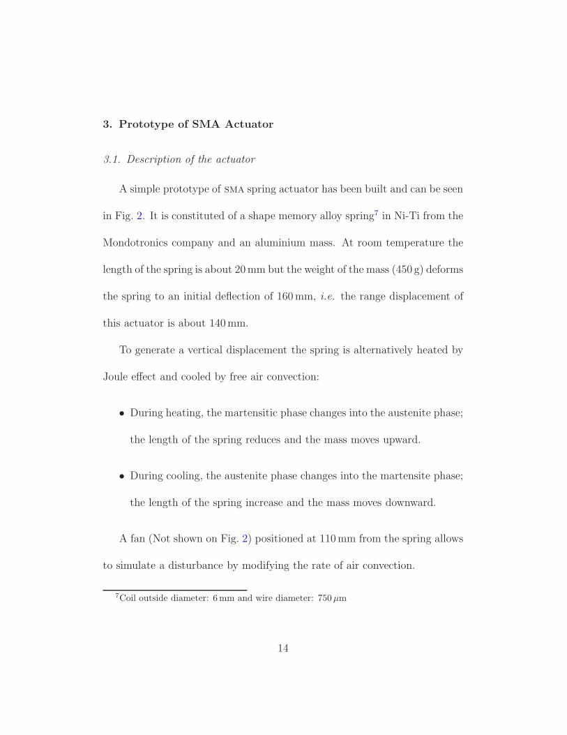
3.1. Description of the actuator

A simple prototype of sma spring actuator has been built and can be seen

in Fig. 2. It is constituted of a shape memory alloy spring7 in Ni-Ti from the

Mondotronics company and an aluminium mass. At room temperature the

length of the spring is about 20mm but the weight of the mass (450 g) deforms

the spring to an initial deflection of 160mm, i.e. the range displacement of

this actuator is about 140mm.

To generate a vertical displacement the spring is alternatively heated by

Joule effect and cooled by free air convection:

• During heating, the martensitic phase changes into the austenite phase;

the length of the spring reduces and the mass moves upward.

• During cooling, the austenite phase changes into the martensite phase;

the length of the spring increase and the mass moves downward.

A fan (Not shown on Fig. 2) positioned at 110mm from the spring allows

to simulate a disturbance by modifying the rate of air convection.

7Coil outside diameter: 6 mm and wire diameter: 750 µm

14

The sma spring is electrically isolated from the frame and a simple elec-

tronic circuit (not shown on Fig. 2) allows to regulated the current flowing

through the spring. The heating current is measured with a shunt preci-

sion resistance and an instrumentation amplifier. The voltage applied to the

spring is also measured with an instrumentation amplifier. The vertical posi-

tion of the mass is measured with a laser sensor8 with a resolution of 0.3mm

over a range of 200mm at a sampling frequency of 100Hz. The actuator

is interfaced to a computer via a data-acquisition board9. The computer

is running under Linux/rtai10 which is a low latency kernel that allows to

implement hard real-time control and measurements from C language codes.

3.2. Position control development

For this application, a first-order local numerical model

y = F + αu (15)

is considered. The choice of a first order comes from the literature about

shape memory alloy modelling in which the order is usually one (see e.g.,

Leclerc and Lexcellent, 1996). The control input u corresponds to the electric

8OWLE 4025 FA S19Humusoft mf–604.

10http://www.rtai.org/

15

Fig. 2. Prototype of a sma spring based actuator.

power crossing the sma spring and the output y is the measured vertical

position of the mass. According to section 2.2, the control is given by:

u =1

α(−[F ]e + y⋆ − Kp(y − y⋆)) (16)

where Kp is a positive gain. Note that as (15) is here first order, a simple

proportional controller is enough to ensure convergence of the error to zero.

Contrarily to classical feedback control there is no need here to add integra-

tors in the stabilisation controller to ensure converge of the position error to

zero as the model free control implicitly involves integrators. This controller

is hence simply called an i-P controller.

16

For comparison purpose, we also have implemented a classical PI control:

u(t) = −KP (y(t) − y⋆(t)) − KI

∫ t

0

(y(τ) − y⋆(τ))dτ (17)

The classic control does involve an integral term in order to avoid static error.

The controller parameters have been manually tuned and are given in

Tab. 1. The dynamic of the process is quite slow and, moreover, the control

effect is “not symmetric” in the sense that there is no control to cool the

sma spring (cooling relies only on free air convection). Consequently, this

is not possible here to apply most of the pi or pid tuning algorithms, like

Ziegler & Nichols rule. So, the tuning of the pi gains have been done in two

steps: Firstly, tuning of the proportional gain on the undisturbed process

(cooling fan off), secondly, tuning of the integral gain in order to achieve a

good perturbation rejection. The obtained gains are, to our best expertise,

the larger we can obtain in order to achieve the trade-off between dynamic

precision and stability.

Similarly, the gains of the i-P controller have been tuned in three steps:

first choose a very large α and a large Kp to have a small steady-state error,

then decrease α to obtain an oscillatory quick response of the system. Fi-

nally decrease Kp to stabilise the system. Note that for step responses, the

first derivative of the trajectory to track, y⋆ equation (16), has been chosen

17

identically zero.

The comparison is laid off in two scenarios presented in the two following

sections.

3.3. First experimental results

3.3.1. Scenario 1 (Fig. 3)

We present classical closed loop step response with thermal disturbance.

In this scenario the mass has to reach a reference position of 70mm. At

time t = 60 s a thermal perturbations is applied using a fan (the effect of

the fan on cooling speed is shown in Fig. 4) and at time t = 90 s the fan is

switched off. Displacement of the mass (output) and electric power crossing

sma spring (input) are plotted in Fig. 3. When the actuator is controlled with

the i-P controller, we observe that the mass reaches the reference position in

approximately 8 seconds without overshoot whereas a 17mm overshoot and

34 s response time are obtained when the actuator is controlled by a classical

pi controller. This overshoot should be reduced (reducing the integral gain)

nevertheless perturbations rejection would be bad. We can observe in Fig. 3-

(a) that the consequence of the thermal perturbation is smaller and rejected

faster by the i-P controller than the pi one. It is clear in Fig. 3-(b) that the

input dynamic is richer when it is calculated by the i-P controller.

18

0

20

40

60

80

100

0 20 40 60 80 100 120

0

2

4

6

8

10

0 20 40 60 80 100 120

outp

ut,

yin

mm

(a)

time, t in s

input,

uin

W

(b) i-P controllerPI controller

Fig. 3. (a): Output vs time for a 70mm step with thermal disturbance when

the actuator is controlled with a i-P and by a pi controller. (b): Correspond-

ing input vs time.

19

0

25

50

75

100

125

150

0 15 30 45 60 75 90time, t in s

outp

ut,

yin

mm

free convection

forced convection (fan)

Fig. 4. Displacement of the actuator vs time during cooling by free and forced

convection (with a fan).

3.3.2. Scenario 2 (Fig. 5)

As the control effect is “not symmetric”, overshoots due to set-point

jumps imply poor performances of the controllers (see for example, the re-

sponse time of the plant with the PI controller). A solution to improve

performances is to generate a transient profile between two set-points that

the output of the plant can reasonably track. So, we present classical poly-

nomial tracking. We can observe that tracking is slightly better when the

actuator is controlled by an i-P (see RMS error and maximal error given in

Fig. 5) however tracking performances are unsatisfactory for the two con-

trollers. A first solution would be to increase the gains of the controllers

20

0

10

20

30

40

50

60

70

80

0 5 10 15 20 25time, t in s

outp

ut,

yin

mm

PI controller

i-P controller

trajectory

Fig. 5. Output vs time during classical tracking when the actuator is con-

trolled with a i-P and by a pi controller.

but for this experiments the choice of gains level results in a trade-off: the

larger are the gains the better are performances in transient however high

level gains degrade performances in steady-state.

We have seen that the i-P controller was able to reject perturbations

faster than the pi controller yet, the tracking performances are slightly dis-

appointing. In the next section, we will modify nonlinear model-free and

PI controllers using a simple off-line nonlinear nonphysical process model

identification. Then we will compare robustness performances of the two

controllers.

21

Table 1. Controllers parameters for experiments of Sec. 3.3.

Kp (proportional gain) Ki (integral gain) α

pi 5 × 10−2 4 × 10−3 –

i-P 0.9 – 600

4. Nonlinear model-free and PI controllers

Nonphysical model process have been used in control and particularly in

industrial applications since many years because models of physical processes

are often difficult to obtain or are too complex to be used in real-time control.

The well known Broıda and Strejc models (linear models with delay) are

very popular and are still used to tune pid controllers (see e.g., Astrom and

Hagglund, 2001; O’Dwyer, 2006; Visioli, 2006). However linear models often

become insufficient for a process with a large operating domain. In this

section, we will see how the use of a very simple nonphysical input-output

model, can improve the control performance of model free control on the SMA

actuator. To provide a fair comparison, we also modify the PI controller in

the same manner, i.e. the control law is applied through a position dependent

gain. This modified PI controller is named as “non linear PI controller” in

22

the sequel.

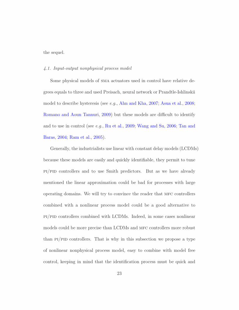
4.1. Input-output nonphysical process model

Some physical models of sma actuators used in control have relative de-

grees equals to three and used Preisach, neural network or Prandtle-Ishlinskii

model to describe hysteresis (see e.g., Ahn and Kha, 2007; Asua et al., 2008;

Romano and Aoun Tannuri, 2009) but these models are difficult to identify

and to use in control (see e.g., Ru et al., 2009; Wang and Su, 2006; Tan and

Baras, 2004; Ram et al., 2005).

Generally, the industrialists use linear with constant delay models (LCDMs)

because these models are easily and quickly identifiable, they permit to tune

pi/pid controllers and to use Smith predictors. But as we have already

mentioned the linear approximation could be bad for processes with large

operating domains. We will try to convince the reader that mfc controllers

combined with a nonlinear process model could be a good alternative to

pi/pid controllers combined with LCDMs. Indeed, in some cases nonlinear

models could be more precise than LCDMs and mfc controllers more robust

than pi/pid controllers. That is why in this subsection we propose a type

of nonlinear nonphysical process model, easy to combine with model free

control, keeping in mind that the identification process must be quick and

23

easy.

For a given order ν, the simplest linear model used to describe a SISO

system is:

y(ν) = −ν−1∑

i=0

Aiy(i) + Bu (18)

where the Ai’s, B and ν are constant parameters. From simulations results,

we found that if B is in fact significantly time varying the MFC controller

yields poor performances. Indeed, in this case, the local model approximation

(equation (12)) is too far from the real behaviour. One of the simplest way to

improve control performances is to enrich the local model with information

about the variations of B. To do so, we first propose a general model which

is an extension of the model (18):

y(ν) = −

ν−1∑

i=0

Aisign(y)|y(i)|ni + g(y)u (19)

where g is a polynomial11 in y, the Ai’s and the ni’s (ni ≥ 1) are constant

parameters which will not be necessary identified as the main information

we need to improve the local model is the knowledge of g. Some example of

response of (19) are given in Fig. 6-(b). The easiest way to identify g is to

use the static relation between the steady-state displacement, yss, and the

11Note that g can also be another kind of function of y.

24

applied constant input uss.

In steady-state equations (19) yields:

− A0 sign(yss)|yss|n0 + g(yss)uss = 0 (20)

Then g(y) =∑s

j=0 ajyj and the parameters A0, n0 are obtained by fitting

the experimental static relation between steady-state output and the corre-

sponding input step. According to equations (20) fitting has been done by

resolving12 the following minimisation problem:

min(A0,n0,aj)

m∑

i=1

((s∑

j=0

ajyjssi

)

ussi− A0y

n0ssi

)2

(21)

where the set (ussi, yssi

) i = 1, · · ·m consists of m measured data pairs where

ui is a constant input and yssi is the corresponding steady-state output. After

some trials, we have found that a polynomial of degree 3 was a good trade

off between model complexity and minimal fitting residue.

g(y) = a0 + a1y + a2y2 + a3y

3 (22)

In Fig. 6-(a) we remark a good correlation between measured data and

simulation. Nevertheless, the obtained solution could be a local minimum

12The authors have chosen a classical quasi-Newton algorithm implemented in Scilab

software

25

and the model has been tested in only one situation. However the idea is

not to obtain an excellent model of the process but just to have some easily-

obtainable insights on its input-output behaviour to design a mfc-based ro-

bust controller and a nonlinear PI controller. Now we will see, how to modify

the two controllers using the identified function g. Then, in Section 4.4, we

will expose some experiments in closed loop.

Remark 2. Some other tests could permit to fully identify the model (19). It

would then be possible to study the stability of this model controlled with the

MFC controller. But as we have already mention, this model is too simple

to describe the entire nonlinear behaviour of the actuator, so it seems that a

stability analysis would be in this case without guarantee on the real stability

of the control on the real plant.

4.2. Design of the nonlinear model-free controller

According to the purely numerical model (equation (12)) identified at

each sample time in mfc and to the previous nonphysical model off line

identified, the new local model becomes:

y = F + αg(y)u

26

0.00

0.03

0.06

0.09

0.12

0.15

0 20 40 60 80 100 120 140

0

2

4

6

8

10

0 2 4 6 8 10 12

steady-state displacement, yss in mm

input,

uin

W

(a)

experimental datasmodel

time, t in s

a = 0.01a = 0.1

u = 2

u = 2

u = 3 u = 3

outp

ut,

y

(b)

Fig. 6. (a): Experimental steady-state output (displacement) as a function of

input compared with our steady-state model. (b): Responses of model (19)

with ν = 1, g(y) = a + y, A0 = 1 and n0 = 1.5 for different values of a and

u (steps).

27

where α ∈ R is a non-physical constant design parameter. The quantity

F ∈ R represents all what is unknown on the system and is updated at each

sampling time, replace α in equation (13) by αg(y). The control is now given

by:

u =1

αg(y)(−[F ]e + y⋆ − Kp(y − y⋆)) (23)

The new control takes advantage of information obtained with the previous

simple nonphysical model and of the robustness of mfc (there is still an

estimation of F at each sampling time).

4.3. Design of the nonlinear PI controller

A simple nonlinear PI controller is simply derived from the classical PI

controller using the previously identified weighting function g(y). It reads:

u(t) =1

g(y)

(

−Kp(y(t) − y⋆(t)) − Ki

∫ t

0

(y(τ) − y⋆(τ))dτ

)

(24)

4.4. Robustness analysis of the two nonlinear controllers

4.4.1. Robustness with respect to thermal disturbance and mass variation

In this subsection, the objective is to test the robustness of the two non-

linear controllers (equations (23) and (24)). Assume that for some set-points,

28

we reasonably want a response time of the plant equals to 10 seconds13. So

we design a polynomial reference trajectory with a transfer time equal to

10 seconds between the two set-points. The controller has to ensure a good

tracking of this trajectory in order to achieve a response time equal to 10

seconds. In the next experiments the trajectories between set-points are

polynomials of degree 5 with zero speed and acceleration at starting and

ending points. We first choose a sixty-seconds scenario in which the 450 g

mass has to reach a steady state level of 65mm with a response time equals

to 10 seconds and to reject a thermal disturbance in steady-state (at time

t = 35 s a thermal perturbations is applied using the fan). Then the gains

adjustment of the two controllers is done manually with the same methods

as those explained in subsection 3.3. The controller parameters are given in

Table 2.

Fig. 7-(a) shows the output of the plant as a function of time after the

tuning procedure. After that, the following sixty-seconds experiments have

been conducted keeping the same controller parameters: from the initial

position, three mass of 280, 360 and 750 have to reach a steady state level

13For the maximal input, the time to browse the entire displacement range is equal to

5 seconds.

29

Table 2. Controller parameters, manually tuned and off-line identified for

experiments of section 4.4.

nonlinear i-P nonlinear PI

Kp 0.7 5.8

α 10 –

Ki – 2.8

a0 0.81 0.81

a1 0.44 0.44

a2 9.19 × 10−3 9.19 × 10−3

a3 2.17 × 10−5 9.19 × 10−3

30

of 20, 40, 60 ,80 and 100 millimetres with a response time of 10 seconds

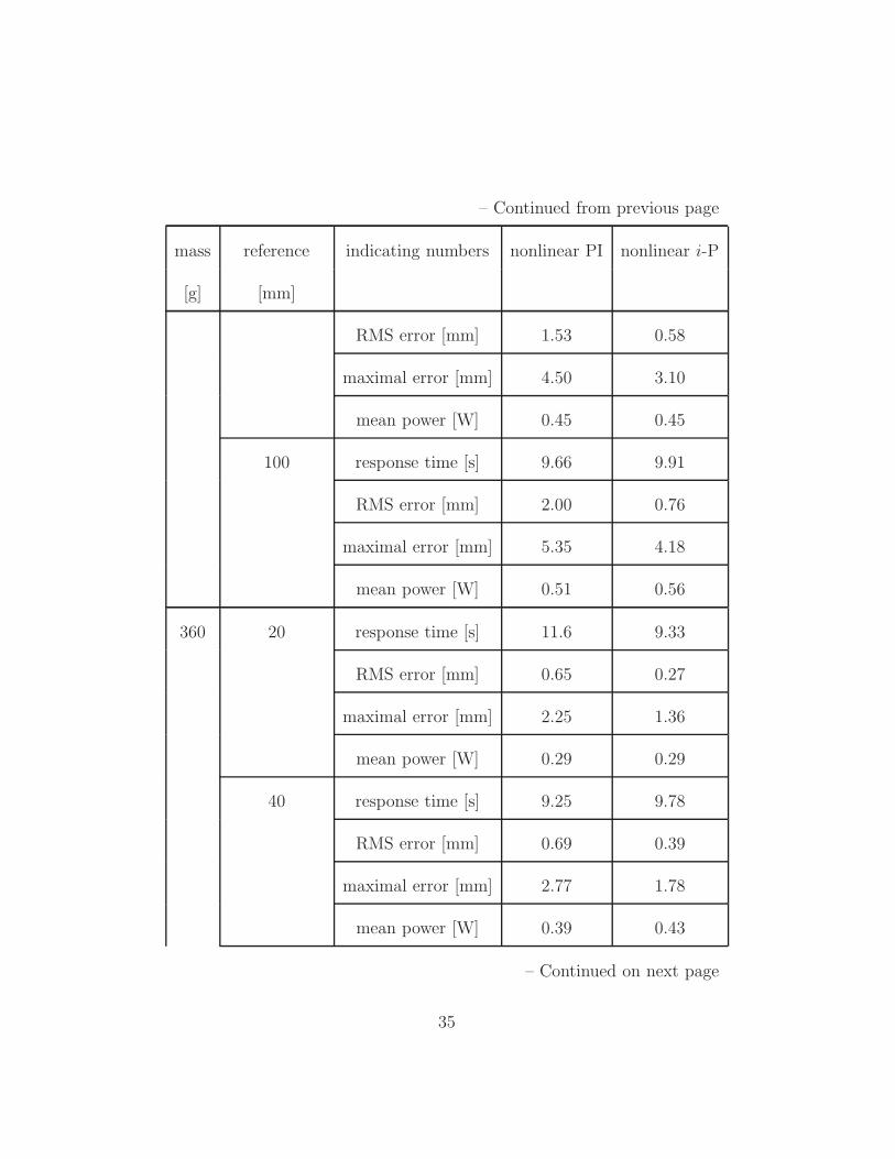
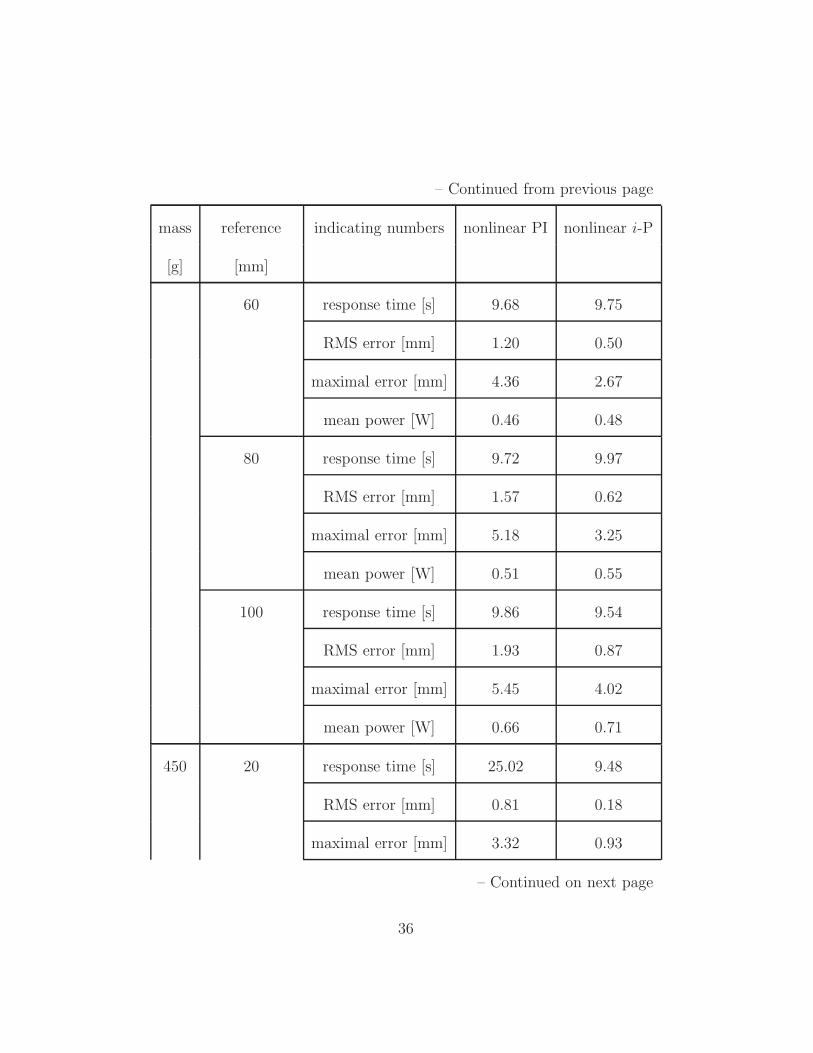
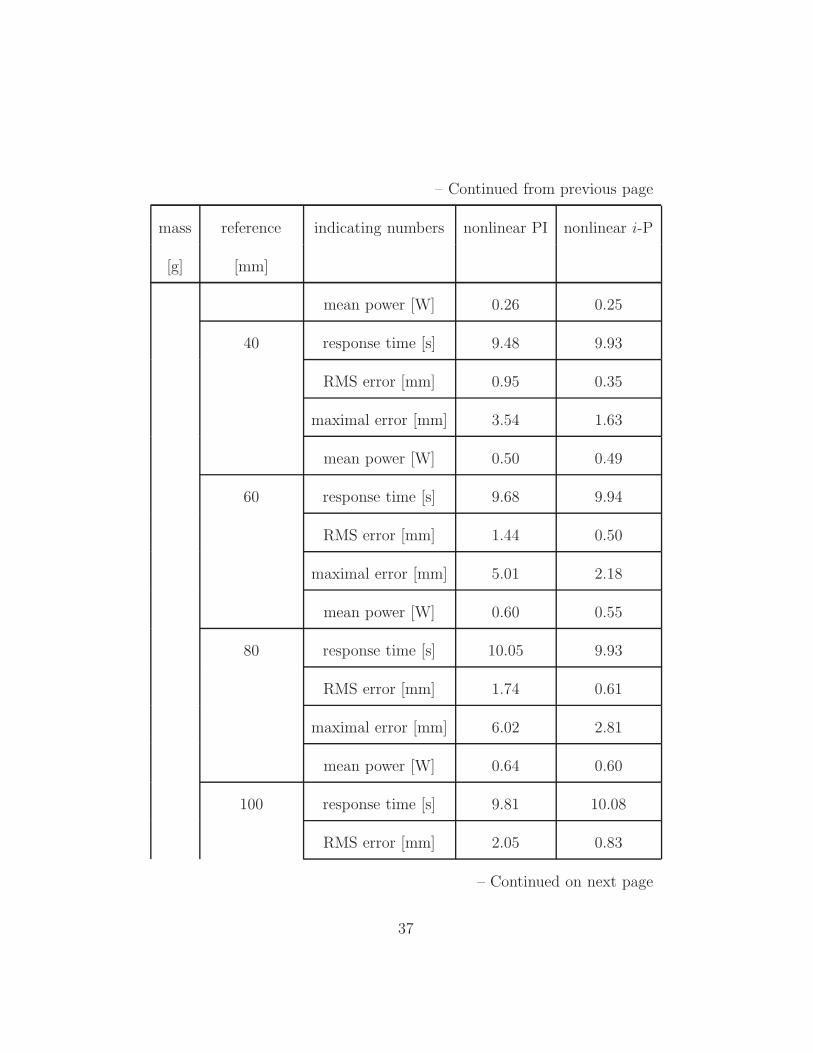
and to reject the thermal disturbance applied at time t = 35 s. To compare

the performances of the two controllers four performance-indicating numbers

have been proposed:

• response time of the plant calculated before the thermal perturbation

(time after which the error is lower than 5% of the total displacement)

• RMS error on t ≥ 10 s

• maximal error on t ≥ 10 s

• mean input power on the whole experiment

These numbers have been calculated for the previously described experiments

and are given table 3.

We can see in Table 3 that the ten-seconds response time is always

achieved in the case of the nonlinear i-P whereas in the nonlinear PI case,

the response time is greater than 10 s in three cases. The RMS error and

the maximal error are smaller for the nonlinear i-P controller. However, the

mean power is often slightly smaller for the nonlinear PI controller than for

the nonlinear i-P controller.

31

0

10

20

30

40

50

60

70

0 10 20 30 40 50 60

0

20

40

60

80

100

120

0 20 40 60 80 100 120 140 160 180 200

(a)

time, t in s

outp

ut,

yin

mm

outp

ut,

yin

mm

(b)

nonlinear PI

nonlinear i-P

Fig. 7. (a): Output vs time for a trajectory with 65mm steady-state level

with thermal disturbance (b): Output vs time for a trajectory which is al-

ternatively increasing or decreasing

32

4.4.2. Robustness with respect to hysteresis effect

A final experiment has been done to test the robustness of the controllers

to hysteresis effects. In this experiment, the output has to track a trajectory

which is alternatively increasing or decreasing. The output of the plant

versus time is shown Fig. 7-(b) for the two controllers. We note that the

performances of the two controllers are still good:

• nonlinear PI case : RMS error = 1.76mm and mean power = 0.14W

• nonlinear i-P case : RMS error = 0.51mm and mean power = 0.13W

From these experiments, we can conclude that a trajectory profile is really

necessary to avoid problems due to set-points jumps and that information

from a very simple model of the plant nonlinearities can improve significantly

the performances of a simple linear feed-back.

33

Table 3. Performance-indicating numbers obtained for experiments of sub-

section 4.4.

mass displacement indicating numbers nonlinear PI nonlinear i-P

[g] [mm]

280 20 response time [s] 13.87 8.05

RMS error [mm] 1.02 0.32

maximal error [mm] 3.18 1.47

mean power [W] 0.23 0.25

40 response time [s] 8.75 9.51









– Continued on next page

34

– Continued from previous page

mass reference indicating numbers nonlinear PI nonlinear i-P

[g] [mm]








360 20 response time [s] 11.6 9.33









35



[g] [mm]













450 20 response time [s] 25.02 9.48




36



[g] [mm]

















37



[g] [mm]



5. Conclusion

The contribution of the paper is twofold: it presents a convincing appli-

cation of the new model-free control in the area of sma actuators control, a

field in which model-based control is especially difficult to develop.

Secondly, in order to improve performances of a i-p and a pi controller, the

paper exposes a general input-output nonphysical model, off-line identified,

which is used to design a nonlinear mfc-based controller and a nonlinear pi

controller.

Experimental results on a sma spring based actuators show good tracking

performances and good robustness towards thermal disturbances and mass

variations for the two controllers. Nevertheless, it seems that the mfc-based

38

controller outperforms nonlinear pi. Finally, we are quite confident to be

able to efficiently control sma micro actuators as micro servo-motors in a

near future.

References

Ahn, K. K., Kha, N. B., 2007. Internal model control for shape memory alloy

actuators using fuzzy based Preisach model. Sensors and Actuators A 18,

141–152.

Ang, K. H., Chong, G., Li, Y., 2005. PID control system analysis, design

and technology. IEEE transactions on control systems technology 13 (4),

559–526.

Arbab Chirani, S., Aleong, D., Dumont, C., McDowell, D., Patoor, E.,

2003. Superelastic behavior modeling in shape memory alloys. Journal de

Physique IV 112, 205–208.

Astrom, K. J., Hagglund, T., 1995. PID Controllers: Theory, Design, and

Tuning, 2nd Edition. Instrument Society of America Press, Research Tri-

angle Park, NC.

39

Astrom, K. J., Hagglund, T., 2001. The future of PID control. Control En-

gineering Practice 9, 1163–1175.

Astrom, K. J., Hagglund, T., 2005. Advanced PID Control. ISA - The In-

strumentation, Systems, and Automation Society, Research Triangle Park,

NC 27709.

Asua, E., Etxebarria, V., Garcia Arribas, A., 2008. Neural network based mi-

cropositioning control of smart shape memory alloy actuators. Engineering

Applications of Artificial Intelligence 21, 796–804.

Benzaoui, H., Chaillet, N., Lexcellent, C., Bourjault, A., 1999. Nonlinear mo-

tion and force control of shape memory alloy actuators. Smart structures

and materials 3667, 337–348.

Bouvet, C., Calloch, S., Lexcellent, C., 2004. A phenomenological model

for pseudoelasticity of shape memory alloys under multiaxial proportional

and nonproportional loadings. European Journal of Mechanics A/Solids

23, 37–61.

Calin, M., Bertsch, A., Chaillet, N., Zissi, S., Ballandras, S., Andre, J. C.,

Bourjault, A., Hauden, D., September 1997. Microrobots realized by mi-

crostereophotolithography and actuated byshape memory alloys. In: Pro-

40

ceedings of the 1997 IEEE/RSJ Intelligent Robots and Systems. Grenoble,

France, pp. 33–34.

Da Silva, E. P., 2007. Beam shape feedback control by means of a shape

memory actuator. Materials and design, Elsevier Science Ltd 28, 1592–

1596.

Dutta, S. M., Ghorbel, F. H., Dabney, J. B., 2005. Modeling and control of a

shape memory alloy actuator. In: International Symposium on Intelligent

Control. Limassol, Cyprus, pp. 1007–1012.

Fliess, M., Join, C., 2009. Model-free control and intelligent PID controllers:

towards a possible trivialization of nonlinear control? In: 15th IFAC Sym-

posium on System Identification (SYSID 2009). IFAC, Saint-Malo France.

URL http://hal.inria.fr/inria-00372325/en/

Fliess, M., Join, C., Mboup, M., Sira-Ramırez, H., 2006. Vers une commande

multivariable sans modele. In: Proc. Conference internationale franco-

phone d’automatique (CIFA’06).

URL http://hal.inria.fr/inria-00001139/fr/

Fliess, M., Join, C., Sira-Ramırez, H., 2008. Non-linear estimation is easy.

International Journal of Modelling, Identification and Control (IJMIC)

41

http://hal.inria.fr/inria-00372325/en/

http://hal.inria.fr/inria-00001139/fr/

4 (1), 12–27.


Fliess, M., Levine, J., Martin, P., Rouchon, P., 1995. Flatness and defect of

non-linear systems: introductory theory and examples. Internat. J. Control

61 (6), 1327–1361.

Gedouin, P.-A., Join, C., Delaleau, E., Bourgeot, J.-M., Arbab Chirani, S.,

Calloch, S., 2008. Model-free control of shape memory alloys antagonistic

actuators. In: 17th IFAC World Congress. Seoul, Korea.

URL http://hal.inria.fr/inria-00261891/en/

Gedouin, P.-A., Join, C., Delaleau, E., Bourgeot, J.-M., Arbab Chirani, S.,

Calloch, S., 2009. A new control strategy for shape memory alloys ac-

tuators. In: 8th European Symposium on Martensitic Transformations

(ESOMAT’09). Prague, Czech Republic.

Gyongy, I., Clarke, D. D., 2006. On the automatic tuning and adaptation of

PID controllers. Control Engineering Practice 14 (2), 149–163.

Hagenmeyer, V., Delaleau, E., 2003a. Exact feedforward linearization based

on differential flatness. Internat. J. Control 76, 537–556.

42


http://hal.inria.fr/inria-00261891/en/

Hagenmeyer, V., Delaleau, E., 2003b. Robustness analysis of exact feedfor-

ward linearization based on differential flatness. Automatica J. IFAC 39,

1941–1946.

Hagenmeyer, V., Delaleau, E., 2008. Continuous-time non-linear flatness-

based predictive control: an exact feedforward linearisation setting with

an induction drive example. Internat. J. Control, 81(10), 1645–1663.

Hagenmeyer, V., Delaleau, E., 2010. Robustness Analysis with Respect to

Exogenous Perturbations for Flatness-Based Exact Feedforward Lineariza-

tion. IEEE Trans. Automatic Control. 55 (3), 727–731

Han, J., 2009. From PID to active disturbance rejection control. IEEE trans-

actions on industrial electronics 56, 900–906.

Janker, P., Claeyssen, F., Grohmann, B., Christmann, M., Lorkowski, T.,

LeLetty, R., Sosniki, O., June 2008. New actuators for aircraft and space

applications. In: 11th International Conference on New Actuators. Bre-

men, Germany.

Jayender, J., Patel, R., Nikumb, S., Ostojic, M., December 2005. H∞ loop

shaping controller for shape memory alloy actuators. In: Proceedings of

43

the 44th IEEE Conference on Decision and Control, and the European

Control Conference 2005. Seville, Spain.

Join, C., Masse, J., Fliess, M., 2006. Commande sans modele pour

l’alimentation de moteurs : resultats preliminaires et comparaisons. In:

Proc. 2e Journees Identification et Modelisation Experimentale (JIME’06).

Poitiers, France.


Join, C., Masse, J., Fliess, M., 2008. Etude preliminaire d’une commande

sans modele pour papillon de moteur. Journal europeen des systemes au-

tomatises (JESA) 42, 337–354.


Khodabakhshian, A., Edrisi, M., 2008. A new robust PID load frequency

controller. Control Engineering Practice 16 (9), 1069–1080.

Kohl, M., Krevet, B., Just, E., 2002. Sma microgripper system. Sens. Actu-

ators A Phys 97-98, 646–652.

Leclerc, S., Lexcellent, C., 1996. A general macroscopic description of the

thermomechanical behaviour of shape memory alloy. Journal of the Me-

chanics and Physics of Solids 44 (6), 953–980.

44



Levine, J., 2009. Analysis and Control of Nonlinear Control Systems: A

Flatness-based Approach. Springer-Verlag, Berlin.

Madill, D. R., Wang, D., July 1998. Modeling and l2-stability of a shape

memory alloy position control system. IEEE Trans. Control Systems Tech-

nology 6 (4), 473–481.

Majima, S., Kodama, K., Hasegawa, T., 2001. Modeling of shape memory

alloy actuator and tracking control system with the model. IEEE Trans.

Control Systems Technology 9, 54–59.

Mboup, M., Join, C., Fliess, M., June 2007. A revised look at numerical

differentiation with an application to nonlinear feedback control. In: 15th

Mediterrean Conference on Control and Automation (MED’07). Athenes,

Greece.


Mboup, M., Join, C., Fliess, M., 2008. Numerical differentiation with anni-

hilators in noisy environment. Numerical Algorithms 50 (4), 439–467.


Mikusinski, J., 1983. Operational calculus, 2nd Edition. PWN & Oxford

University Press.

45



O’Dwyer, A., 2006. Handbook of PI and PID controller tuning rules, 2nd

Edition. Imperial College Press.

Panagopoulos, H., Astrom, K. J., Hagglund, T., 2002. Design of PID con-

trollers based on constrained optimisation. IEE Proceedings - Control The-

ory & Applications 149 (1), 32–40.

Patoor, E., Eberhardt, A., Berveiller, M., 1994. Micromechanical modelling

of the shape memory behavior. Mechanics of phase transformation and

shape memory alloys 189, 23–37.

Peirs, J., Reynaerts, D., Van Brussel, H., June 2002. A retrospective evolu-

tion of a sma microactuation. In: Proceedings of The International confer-

ence on new actuator. Bremen, Germany, pp. 77–80.

Ram, V., Xiaobo, T., P.S., K., June 2005. Approximate inversion of the

Preisach hysteresis operator with application to control of smart actuators.

IEEE Trans. Automatic Control 50 (5), 798–809.

Reger, J. and Jouffroy, J. 2008. Algebraische Ableitungsschatzung im Kon-

text der Rekonstruierbarkeit. Automatisierungstechnik, 58, 324–331.

Romano, R., Aoun Tannuri, E., 2009. Modeling, control and experimental

46

validation of a novel actuator based on shape memory alloys. Mechatronics

In Press, Corrected Proof.

Ru, C., Chen, L., Shao, B., Rong, W., Sun, L., 2009. A hysteresis compen-

sation method of piezoelectric actuator: Model, identification and control.

Control Engineering Practice In Press, Corrected Proof.

Shameli, E., Alasty, A., Salaarieh, H., 2005. Stability analysis and nonlinear

control of a miniature shape memory alloy actuator for precise applications.

Mechatronics 15, 471–486.

Sira-Ramırez, H., Agrawal, S. K., 2004. Differentially Flat Systems. Marcel

Dekker, New York (NJ).

Sittner, P., Vokoun, D., Dayananda, G. N., Stalmans, R., 2000. Recovery

stress generation in shape memory ti50ni45cu5 thin wires. Materials Science

and Engineering A 286, 298–311.

Song, G., Chaudhry, V., Batur, C., 2003. Precision tracking control of shape

memory alloy actuators using neural networks and sliding mode based

robust controller. Smart materials and structures 12, 223–231.

47

Tan, X., Baras, J. S., 2004. Modeling and control of hysteresis in magne-

tostrictive actuators. Automatica 40, 1469–1480.

Tavakoli, S., Griffin, I., Fleming, P. J., 2006. Tuning of decentralised PI (PID)

controllers for TITO processes. Control Engineering Practice 14 (9), 1069

–1080.

Visioli, A., 2005. Design and tuning of a ratio controller. Control Engineering

Practice 13, 485–497.

Visioli, A., 2006. Practical PID Control. Advances in Industrial Control.

Springer, London (UK).

Wang, Q., Su, C.-Y., 2006. Robust adaptive control of a class of nonlinear

systems including actuator hysteresis with Prandtl-Ishlinskii presentations.

Automatica 42, 859–867.

Zehetner, J. Reger, J. Horn, M., 2007. A Derivative Estimation Toolbox

based on Algebraic Methods - Theory and Practice. IEEE 2007 Multi-

conference on Systems and Control (MSC 2007). Singapore.

Zehetner, J. Reger, J. Horn, M., 2007. Echtzeit-Implementierung eines alge-

48

braischen Ableitungsschtzverfahrens. Automatisierungstechnik, 55, 553–

560.

49

Documents

Experimental comparison of classical pid and model-free control