Experimental Design of a Shock Tube

For the Time Response Study of Porous Pressure-Sensitive Paint

Thesis

Presented in Partial Fulfillment of the Requirements for Graduation with Distinction in

the College of Engineering of the Ohio State University

By

David Huynh

Undergraduate Program in Aeronautical and Astronautical Engineering

The Ohio State University

2013

Honors Thesis Committee:

Professor James Gregory, Advisor

Professor Mei Zhuang

Copyright by

David Huynh

2013

ii

Abstract

This thesis summarizes the experimental design of a shock tube apparatus to study the

time response of porous pressure sensitive paint (PSP). PSP is a relatively modern

optical pressure measurement technique that is capable of providing nearly continuous

surface pressure data. The recently developed porous PSP has exhibited very fast

response times, on the order of microseconds, and is thus primed for application in

unsteady flow studies. Much effort has been put into fully characterizing the dynamic

response of porous PSP to most appropriately utilize it in future studies. This research

was aimed to design and construct a shock tube for the purpose of later experimental

evaluation of the time response of porous PSP and other PSP formulations. While the

shock waves generated by shock tubes are commonly used to calibrate the response of

fast instrumentation, this work looked to make use of the contact surface to study the

PSP’s response to pressure increases and pressure decreases. While there were many

challenges in the design process and still many to overcome, the overall design of the

shock tube was successful. Through continued development the device will be a fully

capable tool for the study of the time response of PSP.

iii

Acknowledgements

I am indebted to my research advisor, Professor James Gregory, who provided me with

the opportunity, support, and guidance to conduct this research. I am incredibly grateful

for the time and resources he has invested in my growth as a researcher and Aerospace

Engineer. I would also like to thank Professor Mei Zhuang for her instruction in my

undergraduate career. I have always appreciated her encouragement and I am very

grateful to have her serving on my Honors Thesis Committee.

I could not have been as successful nor learned as much through the course of my

research had it not been for the support of the graduate and undergraduate students in my

research lab. I would like to thank graduate students Samik Bhattacharya, Kevin

Disotell, Kyle Gompertz, Matt McCrink, and Di Peng as well as undergraduate students

Matt Frankhouser, Kyle Hird, and Ryan McMullen for their roles in my undergraduate

development.

I have been blessed with the unwavering support of my parents, Kim Pham and Hung

Huynh, and girlfriend, Nikky Singhal, and I am truly grateful for their contributions to

my progress.

Lastly, I would like to thank the College of Engineering for providing a scholarship in

support of my research work.

iv

Vita

January 18, 1991 ............................................Born, North Olmsted, Ohio, USA

May 5, 2013 ...................................................B.S., Aeronautical and Astronautical

Engineering, The Ohio State University

Field of Study

Major Field: Aeronautical and Astronautical Engineering

v

Table of Contents

Abstract ........................................................................................................................................... ii

Acknowledgements ........................................................................................................................ iii

Vita ................................................................................................................................................. iv

Table of Contents ............................................................................................................................ v

List of Figures ............................................................................................................................... vii

List of Tables ............................................................................................................................... viii

Nomenclature ................................................................................................................................. ix

Chapter 1: Introduction .................................................................................................................. 1

Chapter 2: Background .................................................................................................................. 3

How PSP Works ............................................................................................................. 3

Conventional PSP vs. Porous PSP .................................................................................. 4

How Shock Tubes Work ................................................................................................. 5

Chapter 3: Experimental Design .................................................................................................... 7

Motivation and Design Challenges for Shock Tube ....................................................... 7

Initial Shock Tube Requirements and Design Decisions ................................................ 8

Preliminary Analytical Study .......................................................................................... 9

First Phase Design: Shock Tube Construction.............................................................. 10

Diaphragm Study: Material and Bursting Method........................................................ 12

Second Phase Design: Contact Surface Detection ........................................................ 14

Chapter 4: Current Experimental Set-up and Preliminary PSP Results ...................................... 18

Integration of PSP into Experimental Set-up ................................................................ 18

Preliminary Results for PSP Time Response Study ..................................................... 21

Chapter 5: Discussion and Conclusions ....................................................................................... 24

Chapter 6: References .................................................................................................................. 27

Appendix A: Shock Tube Theory ................................................................................................. 28

vi

Appendix B: MATLAB Code ....................................................................................................... 30

Appendix C: Photographs of Experimental Set-up ....................................................................... 33

vii

List of Figures

Figure 1: Illustration of how PSP operates ......................................................................... 4

Figure 2: Illustration of porous PSP (top) vs. conventional PSP (bottom) ......................... 5

Figure 3: Illustration of a shock tube .................................................................................. 5

Figure 4: Illustration of the changes in static air properties................................................ 6

Figure 5: x-t diagram for Ldriver/Ldriven yielding ................................................................ 10

Figure 6: Kulite data at the end of driven section for first iteration shock tube ............... 12

Figure 7: Kulite data at test section for lengthened driven section ................................... 12

Figure 8: Illustration of nichrome wire across diaphragm ................................................ 14

Figure 9: Kulite (blue) and total pressure pitot probe (red) .............................................. 15

Figure 10: Photodetector data (blue) with predicted contact time (red) ........................... 17

Figure 11: Photodetector (blue), Kulite (red), and predicted contact time (green) ........... 17

Figure 12: Photodetector (blue) and predicted contact time (red), zoomed in to contact

surface prediction .............................................................................................................. 17

Figure 13: Photodetector data, multiple runs .................................................................... 17

Figure 14: Photograph of test section painted with PSP ................................................... 18

Figure 15: Current experimental set-up ............................................................................ 19

Figure 16: PSP (blue) and predicted contact time (red) .................................................... 22

Figure 17: PSP data, zoomed to shock wave .................................................................... 22

Figure 18: PSP (blue), Kulite (red), predicted contact time (green) ................................. 22

Figure 19: PSP (blue), photodetector (red), and predicted contact time (green) .............. 23

Figure 20: PSP and photodetector, zoomed near predicted contact time ......................... 23

viii

List of Tables

Table 1: Summary of experimental configurations to control change gas composition

across contact surface ....................................................................................................... 21

ix

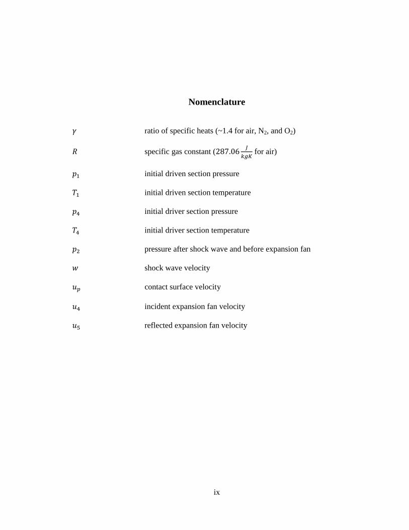
Nomenclature

ratio of specific heats (~1.4 for air, N2, and O2)

specific gas constant (

for air)

initial driven section pressure

initial driven section temperature

initial driver section pressure

initial driver section temperature

pressure after shock wave and before expansion fan

shock wave velocity

contact surface velocity

incident expansion fan velocity

reflected expansion fan velocity

1

Chapter 1: Introduction

In aerodynamic studies of complex flow, pressure distributions provide invaluable insight

on unsteady phenomena. However, traditional pressure transducers provide only discrete

pressure data, severely limiting the resolution of these distributions. In response to this

limitation, an optical pressure measurement technique has recently been developed called

pressure-sensitive paint (PSP). The paint responds to oxygen pressure and can provide

continuous surface pressure data, a significant advantage over pressure transducers.

Conventional PSP was limited by its slow time response, and further developments in

PSP have led to a novel, porous binder that allows for very fast response times, on the

order of microseconds. This porous PSP has many potential applications in unsteady

aerodynamic studies. To best apply the technique, it is crucial to fully characterize how

quickly and the manner in which the paint to responds to a change in pressure, referred to

as its time response.

The long-term goals of this project are to study the time response of various formulations

of porous PSP. The objective of this undergraduate research was to construct a shock

tube apparatus to perform such studies in the future and gather preliminary data. Shock

tubes create high-speed shock waves which are commonly used to calibrate fast-response

instrumentation. However, this study aimed to utilize the contact surface generated by

the shock tube to study the PSP’s time response, an approach with many new benefits and

challenges. One of the novel goals of this apparatus is to test the paint’s response to a

2

rapid pressure decrease, which is typically very difficult to simulate and thus few studies

have included this in their characterization. A great deal was learned during the design

process of the shock tube and preliminary results indicate that there may be significant

difference between the tested PSP’s response to pressure increases and pressure

decreases. The shock tube could provide a simple and effective method of studying PSPs

in the future, which would bring the technique one step closer to becoming a ground-

breaking tool in unsteady flow studies.

3

Chapter 2: Background

How PSP Works

PSP is an optical pressure measurement technique that consists of luminescent particles,

called luminophores, embedded in an adhesive binder matrix. The luminophores can be

brought from their ground state to a higher energy state by being exposed to an excitation

light, typically via laser or LED (light-emitting diode). The particles then return to their

ground state by one of two processes: luminescence, by which the luminophores release

the energy as light, or oxygen quenching, whereby nearby oxygen molecules interact with

and absorb the energy from the luminophores and prevent luminescence. The oxygen

quenching phenomenon is what makes PSP a unique and powerful pressure measurement

technique; at low pressures, fewer oxygen molecules are pressed the model surface,

resulting in less oxygen quenching and thereby more luminescence, while at high

pressures, more oxygen quenching and less luminescence occurs. This process is

illustrated in Figure 1. Surface pressure can thus be inversely related to the paint’s

luminescent intensity. Because pressure measurements can be taken anywhere the PSP is

applied, the paint offers a nonintrusive method to obtain highly spatially resolved surface

pressure data as long as the model is optically accessible.

4

Figure 1: Illustration of how PSP operates

Conventional PSP vs. Porous PSP

Conventional PSPs use a polymer as the binder matrix material. In these paints, oxygen

molecules must diffuse through the polymer binder before being able to interact with the

luminophores, restricting the paints’ response time. Conventional PSPs have been

observed to have response times on the order of seconds, which, while suitable for steady

flow studies, is not suitable for unsteady aerodynamic studies. In response to this

limitation, significant efforts were made to create new binders to allow for faster response

times. As a result, a binder was developed in which the luminophores sit on the surface

of pores in the material, as illustrated in Figure 2. This porous PSP allows the

luminophores to interact directly with local oxygen molecules, resulting in response times

on the order of microseconds (Sakaue 2001). However, as previously mentioned, it is

critical to fully understand the time response characteristics of porous PSP in order to

best apply it. While previous studies have evaluated the response of porous PSP to rapid

increases in pressure, simulating a rapid decrease in pressure is challenging. Thus,

paint’s response to a rapid decrease in pressure still remains to be characterized.

Luminescence

O2

quenching

Low pressure

High pressure

Excitation light

Luminophores

Oxygen

Vs.

5

Figure 2: Illustration of porous PSP (top) vs. conventional PSP (bottom)

How Shock Tubes Work

Shock tubes are popular devices to evaluate the dynamic response of instrumentation. A

shock tube is a long tube, made up of a high-pressure driver section and low-pressure

driven section separated by a diaphragm, illustrated in Figure 3.

Figure 3: Illustration of a shock tube

Traditionally the driver section is referred to as upstream of the diaphragm and the driven

section downstream. When the diaphragm material is broken, either by pressure

difference or alternate mechanism, the resulting instantaneous pressure ratio generates a

downstream-traveling shock wave and an upstream-traveling expansion fan. The

interface between the driver and driven gases induced by the shock wave, called the

6

contact surface, also propagates downstream following the shock. All of the phenomena

travel very quickly, with the shock wave and expansion wave traveling faster than the

speed of sound and the contact surface capable of Mach 0.3-0.5, depending on the initial

pressure ratio (Anderson 2004).

The shock wave provides a nearly instantaneous step change increase in pressure,

temperature, and density. Properties change continuously over the expansion fan. The

contact surface has a step change in temperature and density across it; however, pressure

and velocity are preserved. The changes in air properties over the shock tube phenomena

are illustrated in Figure 4. The speeds and strengths of these shock tube phenomena are

functions of the initial pressure ratio across the diaphragm, defined as driver pressure (p4)

divided by driven pressure (p1). Note this is pressure ratio (p4/p1), not pressure difference

(p4 - p1).

Figure 4: Illustration of the changes in static air properties

(top to bottom: temperature, T; density, ρ; pressure, p) across the shock tube phenomena

Diaphragm

Expansion fan

Contact surface

Shock wave

7

Chapter 3: Experimental Design

Motivation and Design Challenges for Shock Tube

Recall that PSP operates based on local oxygen pressure. This means a change in

pressure for the PSP can be generated by an actual change in pressure or by a change in

oxygen concentration. Exploring the latter observation, this indicates that a pressure

decrease can be simulated by reducing oxygen concentration. Enter the shock tube and

the generated contact surface. The contact surface is a high-speed interface between the

driver and driven gas. If the driver and driven gas were at different oxygen

concentrations, the contact surface would simulate a rapid pressure change as it passed

across the PSP. This would allow for a study of the time response of a PSP sample for

both rapid pressure rises and falls by having the driver and driven sections with different

gas compositions/oxygen concentrations.

While in principle this concept is very simple, there several factors that complicate the

design of this shock tube apparatus. Many difficulties stem from the contact surface,

which is heavily affected by viscosity and boundary layer effects (Mirels 1963) as well as

diaphragm bursting characteristics (Rothkopf 1974). These effects result in the contact

surface being distorted and non-uniform, making the change in test gas composition less

rapid and less consistent. The diaphragm and bursting mechanism are significant

challenges as most previous work with shock tubes has been conducted with high

pressure ratios and thus much stronger and robust diaphragms. A design choice of this

8

research was to operate at low pressure ratios, for safety, convenience, and cost

considerations. Thus, the diaphragm material and bursting mechanism for this project

had to be studied without much of a base from previous work.

Initial Shock Tube Requirements and Design Decisions

The initial concept of the experimental set-up was an inexpensive, “table-top” shock tube,

around or less than 2 meters (~6.5 feet) in length. This size of shock tube was on the

scale of the apparatus used by Sakaue et. al (Sakaue 2001), and so Sakaue’s device was

used as a baseline design. Sakaue’s shock tube was about 1 meter (~3.3 feet) and

operated with the driver section at ambient pressure (~14.7 psi) and the driven section

vacuumed to a desired low pressure (~3.71 psi). Sakaue ran at a pressure ratio of 4 and

broke an aluminum diaphragm via pressure difference.

The initial length of this study’s shock tube was selected to be 5 feet. It was found that

PVC piping was an inexpensive and suitable material for the experiment’s needs, able to

support 200 psi (Home Depot n.d.), significantly greater than the expected experimental

pressures. Using PVC piping restricted the cross section of the tube to be circular. A key

design choice was making the shock tube open-ended at the end driven end. This

decision was motivated by the thought that the generated shock wave would exit the

shock tube and not be reflected, allowing more test time for the contact surface. The

initial driven section pressure was thus constrained to be ambient pressure. Also, with

the driven section open, the driver section would have to be pressurized to create the

desired pressure ratio. With the shock wave exiting the shock tube, it was decided to

keep the pressure ratio fairly low, around 2, to reduce the shock strength of safety

9

concerns. A lower pressure ratio also allowed the shock tube to consume less pressurized

gas, reducing costs.

Preliminary Analytical Study

With the total length of the shock tube and pressure ratio selected, the appropriate lengths

of the driver and driven sections was calculated using the 1-D, inviscid theory presented

by Anderson (Anderson 2004). See Appendix A for a brief description of the theory.

This theory was used to determine the shock wave, contact surface, and expansion fan

velocities given an initial pressure ratio. These velocities were then applied to the shock

tube. The limiting factors on the test time of the shock tube were the time between

passages of the shock wave and the contact surface through the test section and the time

between the passages of the contact surface and the expansion fan through the test

section, which for convenience will be referred to as t1 and t2, respectively. t1 needed to

be large enough to allow the PSP to fully respond to the step change across the shock

wave and t2 need to be large enough to record the PSP’s response to the contact surface

before the expansion fan passed and introduced a gradual pressure decrease.

It was decided that t1 and t2 would be made equal to temporally isolate the contact surface

from the other pressure phenomena. A MATLAB script was written to iterate through

various driver/driven length ratios and calculate the corresponding shock tube velocities

and test time to yield the maximum test time. See Appendix B for the MATLAB code.

The optimal driver/driven ratio was determined to be roughly 0.75/0.25, or 3.75 feet/1.25

feet for a 5 foot tube for a pressure ratio of 2. The corresponding x-t diagram, illustrating

the spatial propagation of the shock tube phenomena through time, is shown in Figure 5.

10

Note that this study assumed that the shock wave would exit the tube and not reflect back

into the driven section.

Figure 5: x-t diagram for Ldriver/Ldriven yielding

maximum test time

First Phase Design: Shock Tube Construction

Using the parameters determined in the preliminary analysis, the first shock tube design

was constructed of 2” inner diameter PVC tubing, with driver and driven lengths 3.75

feet and 1.25 feet, respectively. A Kulite pressure transducer was placed perpendicular to

the flow at the end of the driven section, where the test section would be placed. The

Kulite data was recorded using a Waverunner oscilloscope. A thin sheet of acetate was

used as the diaphragm material and a pointed, metal rod was used as the bursting

mechanism. A more detailed study of the diaphragm material and bursting mechanism

was performed later and is described in the following section. A rapid spike in pressure

t1

t2

Expansion fan (head)

Expansion fan

(tail)

Contact

surface

Shock wave

PSP

11

was observed, shown in Figure 6, which was contrary to the expected step change in

pressure as described in the Background section. This was reasoned to be the result of

ambient air rushing in to return the driven section to ambient pressure after the shock

exited.

In response, an additional 5 feet was added downstream of the test section to prolong this

pressure equalization passed the time window of interest. Looking at Figure 7, it is clear

that the additional tubing allowed the increase in pressure to be sustained. Here, the

shock wave and the expansion fan are clearly resolved; recall that pressure does not

change across the contact surface and thus the contact surface is not represented in the

Kulite data. The slight bump in the expansion fan around 9 ms was the result of a second

expansion fan propagating back upstream into the shock tube. This second expansion fan

was generated as the initial shock wave exited the driven section; as the shock wave left

the tube, the pressurized air just upstream of the shock interacted with the ambient air,

analogous to a second diaphragm burst. This second interaction formed a second

expansion fan traveling back into the shock tube, which collided with and added to the

first expansion. This explanation was arrived at through experimental results as well as

computational results from a second-order upwind scheme (Huynh 2003) and was

eventually supported by literature from previous shock tube studies (Gordon/Hall 1959).

12

Figure 6: Kulite data at the end of driven section

for first iteration shock tube

Figure 7: Kulite data at test section for lengthened

driven section

Diaphragm Study: Material and Bursting Method

Potentially the most critical aspect of the shock tube design was the diaphragm material

and bursting method. This is because previous shock tube studies have shown that the

planarity and quality of the contact surface are heavily dependent on the diaphragm

characteristics. In basic shock tube theory, when the diaphragm is burst, it

instantaneously and uniformly disappears. In reality, the most ideal diaphragm bursts

into the four-pedal formation, where the four equal pedals simultaneously fold out flush

to the tube walls. This type of burst has been observed to generate the most uniform

shock waves and contact surfaces (Rothkopf 1974). In addition to the uniform

phenomena, the four-pedal burst also retains the diaphragm, with no shrapnel traveling

downstream. This aspect was important because the PSP study requires constant optical

access. If the four-pedal formation was not achievable, it was determined that upon

Shock wave

First expansion fan

Second expansion

fan

13

bursting, as much area from the diaphragm should break as quickly as possible, with

minimal material traveling down the shock tube.

Three diaphragm materials were considered: metallic dura-lar film (the material of

metallic balloons), acetate (thin, transparent plastic; similar to overhead projector slides),

and aluminum foil. Likewise, three bursting methods were evaluated: bursting via

physical plunger, heating, and pressure difference. The plunger used was a pointed,

metal rod. The heating method entailed a thin nichrome wire making contact with the

diaphragm, through which a current was applied, heating the nichrome wire and

weakening the diaphragm to the point that the pressure broke the material.

The dura-lar film was ruled out because the material was too strong and did not burst

even after being punctured with the plunger. The aluminum foil proved to be too weak as

it tended to break into many pieces and travel downstream. Though the plunger was a

very simple and consistent mechanism to break the diaphragm, it was a significant body

in the flow and could also limit optical access to the test section and so was not selected.

Bursting via pressure difference was found to be inconsistent and, with the exception of

aluminum foil, required a large driver pressure to break the diaphragm. Thus, the

diaphragm material was chosen to be acetate and the bursting mechanism heating through

a nichrome wire.

The nichrome wire was stretched across the downstream end of the acetate sheet. This

way, when the acetate bulged from the driver section pressure, it would be pressed into

contact with the wire. Upon bursting, the acetate did not fold into the four-pedal

formation; like the aluminum, the acetate tended to tear. However, the acetate was

stronger than the aluminum and tore into fewer, larger pieces. By simply applying an

14

adhesive to the acetate, when the diaphragm burst, the material would tear, flap open, and

the torn shrapnel would be retained by the tape. Multiple nichrome wire orientations

were explored: the nichrome was stretch across a diagonal, across a secant, around the

circumference, and in a cross. The secant-orientation, illustrated in Figure 8, was found

to be the best positioning as it consistently removed the greatest amount of material upon

bursting.

Figure 8: Illustration of nichrome wire across diaphragm

Second Phase Design: Contact Surface Detection

After determining the diaphragm apparatus and acquiring consistent pressure data, the

test section for the PSP was added to the shock tube. A 2” inner diameter cast acrylic

tube was selected for the test section for its transparency and machinability. The acrylic

was cut to a 1.5” length; the short length was necessary in order to paint the inside of the

section. However, before the PSP was integrated into the experiment, an extensive study

was performed on the contact detection.

Nichrome wire

Inner diameter Outer diameter

Adhesive for shrapnel retention

15

Detection of the contact surface was by far the most challenging aspect of the design.

Because static pressure and velocity are constant across the contact, only instrumentation

sensitive to total pressure, temperature, or density were applicable. All temperature

sensors that were considered were found to be too slow (thermocouples), too fragile (hot

wires), or too expensive (infrared temperature sensors). A total pressure pitot probe was

tested and displayed a fast enough response to capture the shock wave; however, the

change in total pressure was too small to be observed, as seen in Figure 9.

Figure 9: Kulite (blue) and total pressure pitot probe (red)

As the density changes, so does the index of refraction; in fact, index of refraction is

related to the spatial gradient of density (Settles 2006). Thus, a small change in density

over a very small distance, such as across a shock or contact surface, there will be large

change in index of refraction. Using this idea, a 532 nm (green) laser diode was

positioned to fire a laser through the test section onto a photodetector. The photodetector

output a voltage corresponding to the spatial position of the laser, with left being more

16

negative and right being more positive. Thus, as the shock wave or contact surface

passed the test section, the increase in density and index of refraction would refract the

laser upstream, which would be registered by the photodetector as a brief and rapid

decrease in voltage (assuming left upstream). Though it would be very difficult to extract

the magnitude of the density gradient across the shock or contact using this method, only

the time data was necessary. The photodetector laser diode was positioned such that the

laser passed through the cross-sectional plane of the Kulite to ensure the signals would be

temporally synchronized.

A representative plot of the photodetector data is displayed in Figure 10, with the

photodetector data in blue and the contact surface prediction from the 1-D theory in red.

The shock wave was well resolved as seen by the sharp spike downward, which

corresponded well to the pressure increase in the Kulite signal in Figure 11. There

appeared to be some slight oscillations in the photodetector near the predicted contact

time, though closer inspection in Figure 12 revealed a noisy signal with no obvious

representation of when contact begins passing through the test section. Moreover,

looking at Figure 13, multiple runs displayed a few common characteristics, such has the

spike corresponding to the shock wave and an increase in oscillations near the predicted

contact surface time, but also very distinct long-time scale patterns. This made the

characterization of the contact surface little more than speculation, as the signal noise

could vary from run to run as well as be a result of a non-uniform contact surface.

17

Figure 10: Photodetector data (blue) with

predicted contact time (red)

Figure 11: Photodetector (blue), Kulite (red),

and predicted contact time (green)

Figure 12: Photodetector (blue) and predicted

contact time (red), zoomed in to contact surface

prediction

Figure 13: Photodetector data, multiple runs

Despite the inconclusive contact detection study, it was decided to proceed to the PSP

phase of the design as it was possible that the PSP’s response could help illuminate the

contact surface.

18

Chapter 4: Current Experimental Set-up and Preliminary PSP Results

Integration of PSP into Experimental Set-up

One fourth of the test section’s circumference was coated in PtTFPP, the paint

formulation used by Dr. James Gregory’s research group at the Aeronautical and

Astronautical Research Labs (see Figure 14 for a photograph). A high-powered 532 nm

laser was selected as the excitation source and a photomultiplier tube (PMT) was selected

as the instrument to record the luminescence. The PSP, laser, and PMT were integrated

into the current experimental set-up, illustrated in Figure 15. See Appendix C for

photographs of the experimental set-up.

Figure 14: Photograph of test section painted with PSP

19

Figure 15: Current experimental set-up

With the PSP in the test section, the driver section was pressurized with nitrogen gas to

simulate the pressure decrease across the contact surface. The excitation laser was

positioned such that the excitation spot was in the same plane with the Kulite and

photodetector laser so all three signals would line up temporally. Because the PMT was

so sensitive to light and could be easily damaged, all data with the PSP was taken with all

doors closed and all lights off except the lasers. Once the optics were set up, the driver

pressure was recorded by the Omega pressure transducer for the analytical contact

prediction. The circuit with the nichrome wire was then closed, heating the wire and

bursting the diaphragm. An oscilloscope recorded the data from the Kulite,

photodetector, and PMT; the system was triggered by the shock wave in the Kulite signal.

To most meaningfully compare the PSP’s time response to a pressure increase to its time

response to a pressure decrease, it was important to keep the magnitude and quality of the

pressure change the same and simply switch the direction. This study utilized the contact

surface as a pressure decrease; the driver section was filled with a pressurized

20

nitrogen/air mixture and the driven section was left open to atmospheric air. For clarity,

this will be referred to as configuration 1, where downstream of the contact is air and

upstream is a nitrogen/air mixture. In consideration of future studies, a process to reverse

the gas composition across the contact surface was devised, which will be referred to as

configuration 2. In configuration 2, the driver section would be pressurized using shop

air to match the driver pressure in configuration 1 (to generate phenomena of equal speed

and strength) and also match the driven oxygen concentration in configuration 1, which

was also air. The driven section in configuration 2 would then be brought to the same

nitrogen/air concentration of the driver section in configuration 1 through a process called

purging. A nitrogen supply and an air supply would each be regulated to the appropriate

pressures to create the desired nitrogen/air ratio. The two supplies would be hosed

together and the gasses allowed to mix. This mixture would then flood the driven

section, downstream of the diaphragm and upstream of the test section. A finite amount

of time would be given for the purging process to fully saturate the driven section with

the mixture. Once saturation was reached, the purging would be stopped and

immediately after the shock tube fired, so as to not allow time for the ambient air to

propagate up the driven section. This would create a contact surface with a downstream

nitrogen/air mixture and upstream air while maintaining the same pressure ratio as

configuration 1, simulating the equivalent pressure increase case to configuration 1’s

pressure decrease. Table 1 summarizes the conceptual set-up for each configuration.

21

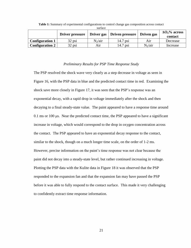
Table 1: Summary of experimental configurations to control change gas composition across contact

surface

Driver pressure Driver gas Driven pressure Driven gas ΔO2% across

contact

Configuration 1 32 psi N2/air 14.7 psi Air Decrease

Configuration 2 32 psi Air 14.7 psi N2/air Increase

Preliminary Results for PSP Time Response Study

The PSP resolved the shock wave very clearly as a step decrease in voltage as seen in

Figure 16, with the PSP data in blue and the predicted contact time in red. Examining the

shock save more closely in Figure 17, it was seen that the PSP’s response was an

exponential decay, with a rapid drop in voltage immediately after the shock and then

decaying to a final steady-state value. The paint appeared to have a response time around

0.1 ms or 100 μs. Near the predicted contact time, the PSP appeared to have a significant

increase in voltage, which would correspond to the drop in oxygen concentration across

the contact. The PSP appeared to have an exponential decay response to the contact,

similar to the shock, though on a much longer time scale, on the order of 1-2 ms.

However, precise information on the paint’s time response was not clear because the

paint did not decay into a steady-state level, but rather continued increasing in voltage.

Plotting the PSP data with the Kulite data in Figure 18 it was observed that the PSP

responded to the expansion fan and that the expansion fan may have passed the PSP

before it was able to fully respond to the contact surface. This made it very challenging

to confidently extract time response information.

22

Figure 16: PSP (blue) and predicted contact

time (red)

Figure 17: PSP data, zoomed to shock wave

Figure 18: PSP (blue), Kulite (red), predicted contact time (green)

Juxtaposing the PSP data with the photodetector data revealed that, if the oscillations in

the photodetector did indicate the contact surface, the PSP had a significant time delay

associated with it. Figure 19 shows the PSP and photodetector data together and Figure

20 shows the oscillations in the photodetector preceded the jump in the PSP by between

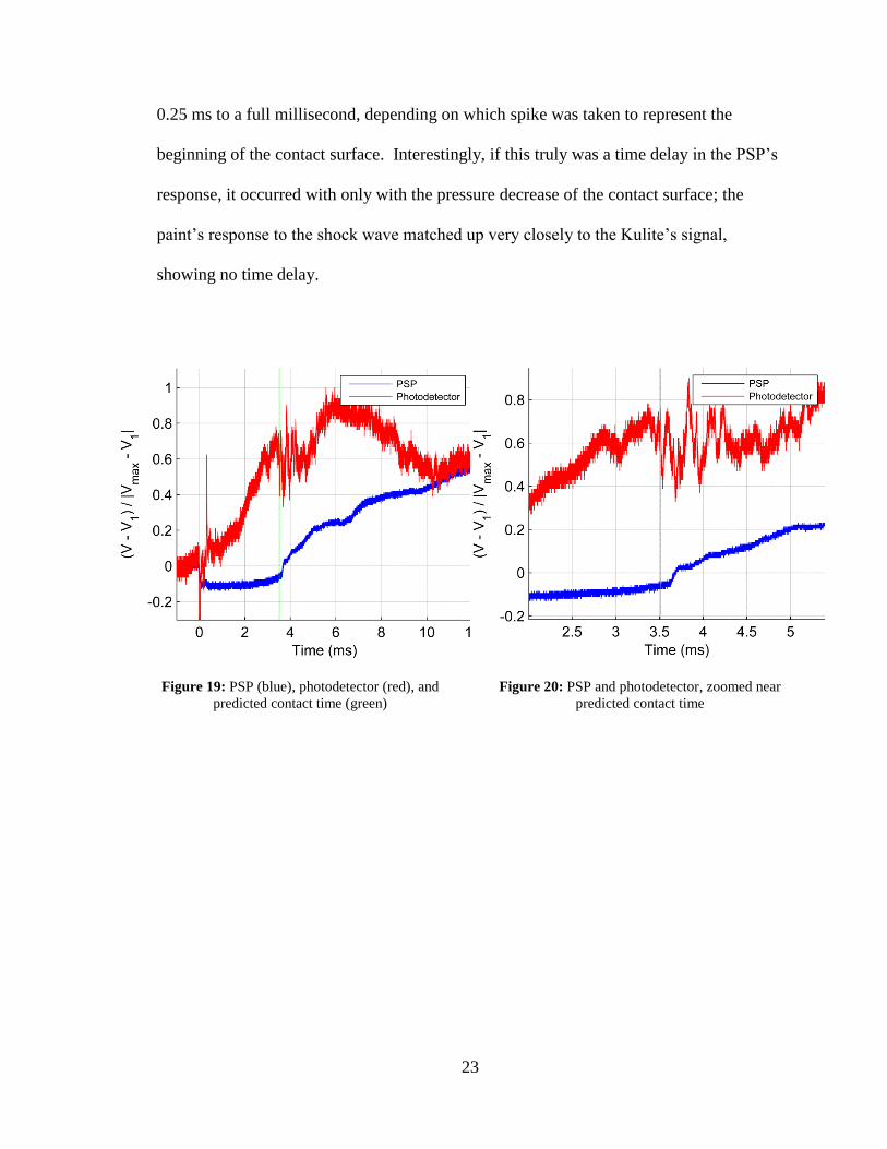
23

0.25 ms to a full millisecond, depending on which spike was taken to represent the

beginning of the contact surface. Interestingly, if this truly was a time delay in the PSP’s

response, it occurred with only with the pressure decrease of the contact surface; the

paint’s response to the shock wave matched up very closely to the Kulite’s signal,

showing no time delay.

Figure 19: PSP (blue), photodetector (red), and

predicted contact time (green)

Figure 20: PSP and photodetector, zoomed near

predicted contact time

24

Chapter 5: Discussion and Conclusions

Designing and constructing the shock tube for future PSP study proved to be a very

challenging and instructive process. The initial design decision to have the driven end be

open to avoid the reflected shock wave was found to be slightly misguided; though the

open end did prevent the shock wave reflection, as the shock exited the tube, it acted like

a second diaphragm burst and sent a second expansion fan traveling back upstream. In

retrospect, a semi-infinite shock tube rather than an open shock tube would have avoided

both the reflected shock wave and second expansion fan, though this has obvious

implementation issues. The second expansion fan did not interfere with the PSP study,

though it was an interesting discovery in the shock tube development.

As predicted, the contact surface presented several challenges to the experimental

method. After eliminating several detection instruments, it was decided that a

photodetector would be used to detect the refraction of a laser through the test section

caused by the change in density over the contact surface. However, it was observed that

the contact was very difficult to identify in the photodetector data due to the noisy signal.

Though there did appear to be some notable patterns in the signal that were suspected to

be the contact surface, it was unclear when the contact surface began. This obscurity

could have been the result of a non-uniform contact surface or a limitation in the

detection method itself.

25

Despite the struggles in contact detection, the preliminary results from the porous PSP

were very promising. The PSP was able to resolve the shock wave and was in close

agreement with the Kulite data. Based on the response to the shock, the PSP appeared to

have a response time on the order of 100 μs, a result in close agreement with results of

previous studies (Gregory et al. 2008 & Sakaue 2001). The PSP also responded to the

contact surface, though much more slowly. It was unclear whether the slow response was

due to the PSP’s limitations or the result of a non-uniform contact surface, making the

analysis of the time response inconclusive. In future studies, it would be beneficial to

operate the shock tube such that there is more time between the contact surface and the

expansion fan to give the PSP more time to respond to the contact surface. This can be

achieved by increasing the pressure ratio across the diaphragm or moving the test section

more upstream.

The shock tube design was successful in a number of ways. The diaphragm and bursting

method provided consistent and controlled operation of the shock tube. The pressure

phenomena were clearly resolved by the Kulite pressure transducer and the shock wave

provided a reliable means of triggering the data acquisition. The test sections were

designed in such a way that they were easily removed from the tube and reused for

different PSP formulations. The shock tube was secured to the table, minimizing recoil

from the diaphragm burst. The PSP data indicated a need to further develop the

apparatus to isolate the contact surface, but was encouraging nonetheless. I am confident

that I will be able to bring the shock tube to full functionality before my graduation this

year.

26

Outside of its application in studies of PSP, the shock tube would be very useful and

instructive as an undergraduate academic lab. Without the optical set-up, the shock tube

was inexpensive, simple to construct, and very illustrative of fundamental compressible

flow. It is my hope that my research can provide future students an opportunity to see

their studies applied.

27

Chapter 6: References

Anderson, J.D. "Modern Compressible Flow With Historical Perspective." 261-302.

McCraw-Hill, 2004.

Gordon/Hall, I. I. Glass and J. "Section 18: Shock Tubes." In Handbook of Supersonic

Aerodynamics. Bureau of Naval Weapons, 1959.

Gregory, J W, K Asai, M Kameda, T Liu, and J P Sullivan. "A review of pressure-

sensitive paint for high-speed and unsteady aerodynamics." Journal of Aerospace

Engineering, 2008: 249-290.

Home Depot. n.d.

http://www.homedepot.com/p/t/100161954?catalogId=10053&langId=-

1&keyword=pvc+pipe+2%22&storeId=10051&N=5yc1v&R=100161954#specifi

cations (accessed June 27, 2012).

Huynh, H.T. "Analysis and improvement of upwind and centered schemes on

quadrilateral and triangular meshes." AIAA Paper 2003-3541, 2003.

Mirels, Harold. "Test Time in Low Pressure Shock Tubes." Physics of Fluids, 1963:

1201-1214.

Rothkopf, E.M. and Low, W. "Diaphragm opening process in shock tubes." Physics of

Fluids, 1974: 1169-1173.

Sakaue, H. and Sullivan, J.P. "Time Response of Anodized Aluminum Pressure-Sensitive

Paint." AIAA 39(10), 2001: 1944-1949.

Settles, G.S. Schlieren & Shadowgraph Techniques. Springer, 2006.

28

Appendix A: Shock Tube Theory

Traditionally, shock tube theory follows the following notation:

Before diaphragm bursts:

After burst, before expansion fan reflection:

After expansion fan reflection:

Given:

Solving for: (shock wave speed), (contact surface speed), (incident expansion

fan speed), (reflected expansion fan speed)

First the initial speeds of sound, and , were determined by:

A1

Where R is the specific gas constant for air (

). The pressure ratio across the

shock wave ( ) was then calculated iteratively through the following:

29

{

( ) ( ) ( )

[ ( ) ( )]

}

A2

With the shock wave pressure ratio, the shock wave speed and contact surface speed were

then calculated using equations A3 and A4, respectively.

√

( ) A3

( )(

)

A4

The expansion fan was analyzed using the method of characteristics of finite nonlinear

waves. For further details, see (Anderson 2004) and the MATLAB script in Appendix B.

30

Appendix B: MATLAB Code

shocktube_refvel: given initial driver and driven conditions, calculate shock wave and

contact surface properties.

function [ w,u_p,p2top1,a4,T2,Ms ] = shocktube_refvel( driver_pressure,... driven_pressure,driver_temp,driven_temp,gamma ) %shock_contact_vel calculates shock wave and contact velocities % shock_contact_vel calculates the velocities of resulting shock wave and % contact of a shock tube. This function receives driver pressure and % temperature, driven pressure and temperature, and ratio of specific % heats of the fluid as input variables. This function operates under the % following assumptions: % 1) The ratio of specific heats is uniform or approximately uniform % across the tube. % 2) The fluid can be considered a calorically perfect gas.

% Previously: [ w,u_p,v_inc,v_ref,x_refexp,t_refexp,p2top1,a4 ] = % shocktube_refvel( driver_pressure,driven_pressure, % driver_temp,driven_temp,gamma,L_driver ) p4=driver_pressure; %initialize variables using input variables p1=driven_pressure; t4=driver_temp; t1=driven_temp;

%R=1716.49; %set universal gas constant (English) R=287.04; %set universal gas constant (metric)

p4top1=p4/p1; %set driver/driven ratio a1= (gamma*R*t1)^.5; %determine driven speed of sound a4= (gamma*R*t4)^.5; %determine driver speed of sound

p2top1=fzero(@(pratio) (-p4top1+pratio*(1-((gamma-1)*(a1/a4)*(pratio-1))... /(2*gamma*(2*gamma+(gamma+1)*(pratio-1)))^.5)^((-2*gamma)/(gamma-1))),... p4top1); %determine p2/p1

%syms pratio %p2top1=solve((-p4top1+pratio*(1-((gamma-1)*(a1/a4)*(pratio-1))... % /(2*gamma*(2*gamma+(gamma+1)*(pratio-1)))^.5)... % ^((-2*gamma)/(gamma-1)))==0); %determine p2/p1 %p2top1=double(p2top1); %p2top1(imag(p2top1)~=0)=[]; %p2top1=max(p2top1);

w= a1*(((gamma+1)/(2*gamma))*(p2top1-1)+1)^.5; %calculate shock speed u_p= a1/gamma*(p2top1-1)*((2*gamma/(gamma+1))/... (p2top1+(gamma-1)/(gamma+1)))^.5; %calculate contact speed

t2tot1=p2top1*((gamma+1)/(gamma-1)+p2top1)/(1+(gamma+1)/(gamma-1)*p2top1); T2=t2tot1*t1; Ms=w/a1;

end

31

refexp: given contact surface speed and initial driver conditions, calculate incident and

reflected expansion fan speeds and generate [x,t] coordinates.

function [ vh_inc,vh_ref,xh,th,vt_inc,vt_ref,xt,tt,a5,u ] = ... refexp( u_p,inc,a4,L_driver ) %REFEXP solves the reflected expansion fan problem for the head and tail % REFEXP uses the method of characteristics to solve the reflected expansion % fan problem and returns velocity, position, and time values for the % head and tail expansion waves. The formatting is as follows % % [vh_inc,vh_ref,xh,th,vt_inc,vt_ref,xt,tt] = refexp(u_p,inc,a4,L_driver) % u_p = contact or piston speed % inc = increment for 0:u_p % a4 = inital speed of sound in driver section % L_driver = length of the driver section % % vh_inc = incident expansion wave head vel (all velocities in m/s) % vh_ref = reflected expansion wave head vel % xh = expansion wave head x location data (all distances in m) % th = expansion wave head time data (all times in microseconds) % vt_inc = incident expansion wave tail vel % vt_iref = reflected expansion wave tail vel % xt = expansion wave tail x location data % tt = expansion wave tail time data % % This code defines n x n matrices for most variables to be calculated at % each point in the reflection, where n is the number of expansion waves: % _ _ 6|/ / / *Note the waves should all start % | 1 2 3 | |\ / / at the same x-axis location % | 0 4 5 | t | 5 / % |_ 0 0 6 _| 4|/ 3 % | 2 \ % 1|/ \ \ % |\__\_\______________ x % The each row represents an expansion wave and the diagonal elements % represent the points at which each wave meets the wall % % In order to utilize the vel=0 condition at the wall, the x-location and % time matrices were (n+1) x n, with the first row being all zeros: % _ _ % | 0 0 0 0 | % | 1 2 3 4 | % | 0 5 6 7 | % | 0 0 8 9 | % |_ 0 0 0 10 _| % % Useful theory: % J+ = u + (2*a)/(gamma-1); J- = u - (2*a)/(gamma-1) % C+ = (dx/dt)+ = u + a; C- = (dx/dt)- = u - a; % J+/J- is constant along C+/C- curves, respectively

gamma=1.4;

vel=0:inc:u_p; %define vector of expansion wave velocities nwaves=length(vel); %determine number of expansion waves x=zeros(nwaves+1,nwaves); %generate zero matrix for x-location t=x; %generate zero matrix for time jp=zeros(nwaves,nwaves); %generate zero matrix for J+ jm=jp; %generate zero matrix for J- u=jp; %generate zero matrix for wave velocity a=jp; %generate zero matrix for speed of sound cp=jp; %generate zero matrix for C+ cm=jp; %generate zero matrix for C-

for i=1:nwaves %cycle through the waves

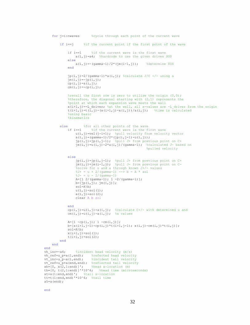
32

for j=i:nwaves %cycle through each point of the current wave

if i==j %if the current point if the first point of the wave

if i==1 %if the current wave is the first wave a(i,j)=a4; %hardcode to use the given driven SOS else a(i,j)=-(gamma-1)/2*(jm(i-1,j)); %determine SOS end

jp(i,j)=2/(gamma-1)*a(i,j); %calculate J/C +/- using a jm(i,j)=-jp(i,j); cp(i,j)=a(i,j); cm(i,j)=-cp(i,j);

%recall the first row is zero to utilize the origin (0,0); %therefore, the diagonal starting with (2,1) represents the %point at which each expansion wave meets the wall x(i+1,j)=-L_driver; %at the wall, all x-values are -L_driver from the origin t(i+1,j)=t(i,j)-(x(i+1,j)-x(i,j))/a(i,j); %time is calculated %using basic %kinematics

else %for all other points of the wave if i==1 %if the current wave is the first wave u(i,j)=vel(j-i+1); %pull velocity from velocity vector a(i,j)=(gamma-1)/2*(jp(i,j-1)-u(i,j)); jp(i,j)=jp(i,j-1); %pull J+ from previous point on C+ jm(i,j)=u(i,j)-2*a(i,j)/(gamma-1); %calculated J- based on %pulled velocity

else jp(i,j)=jp(i,j-1); %pull J+ from previous point on C+ jm(i,j)=jm(i-1,j); %pull J- from previous point on C- %solve for u and a through known J+/- values %J+ = u + 2/(gamma-1) --> b = A * sol %J- = u - 2/(gamma-1) A=[1 2/(gamma-1); 1 -2/(gamma-1)]; b=[jp(i,j); jm(i,j)]; sol=A\b; u(i,j)=sol(1); a(i,j)=sol(2); clear A b sol

end cp(i,j)=u(i,j)+a(i,j); %calculate C+/- with determined u and cm(i,j)=u(i,j)-a(i,j); %a values

A=[1 -cp(i,j); 1 -cm(i,j)]; b=[x(i+1,j-1)-cp(i,j)*t(i+1,j-1); x(i,j)-cm(i,j)*t(i,j)]; sol=A\b; x(i+1,j)=sol(1); t(i+1,j)=sol(2); end end end vh_inc=-a4; %incident head velocity (m/s) vh_ref=u_p+a(1,end); %refected head velocity vt_inc=u_p-a(1,end); %incident tail velocity vt_ref=u_p+a(end,end); %reflected tail velocity xh=[0, x(2,1:end)]'; %head x-location (m) th=[0, t(2,1:end)]'*10^6; %head time (microseconds) xt=x(1:end,end)'; %tail x-location tt=t(1:end,end)'*10^6; %tail time a5=a(end);

end

33

Appendix C: Photographs of Experimental Set-up

Figure C1: Full shock tube

Figure C2: Omega pressure transducer for measuring driver section pressure

Omega

transducer

34

Figure C3: Diaphragm region with nichrome wire stretch across

Figure C4: Acetate sheet applied to diaphragm region

Nichrome

wire

35

Figure C5: Laser diode and photodetector set-up

Figure C6: Laser diode and photodetector set-up, lights off

Photodetector

Laser diode

36

Figure C7: High-powered laser and PMT set-up

Figure C8: High-powered laser and PMT set-up, lights off

High-powered

laser

PMT