Experimental Forecasts of Indian Ocean Dipole using a Coupled

OAGCM

JING-JIA LUO

Frontier Research Center for Global Change, JAMSTEC, Yokohama, Japan

SEBASTIEN MASSON

LOCEAN - IPSL, Univ. Pierre et Marie Curie, Paris, France

SWADHIN BEHERA AND TOSHIO YAMAGATA∗

Frontier Research Center for Global Change, JAMSTEC, Yokohama, Japan

J. Climate (Submitted: 7 April 2006; accepted: 11 October 2006)

Corresponding author address:

Jing-Jia Luo

Frontier Research Center for Global Change, JAMSTEC, 3173-25 Showa-machi, Kanazawa-ku,

Yokohama, Kanagawa 236-0001, Japan.

E-mail: luo@jamstec.go.jp; Tel: +81-45-778-5513; Fax: +81-45-778-5707

∗Also affiliated with Department of Earth and Planetary Science, The University of Tokyo, Tokyo,

Japan

0

Abstract

The Indian Ocean Dipole (IOD) has profound socio-economic impacts on not only the

countries surrounding the Indian Ocean but also various parts of the world. A forecast

system is developed based on a relatively high resolution coupled ocean-atmosphere GCM

with only sea surface temperature (SST) information assimilated. Retrospective ensemble

forecasts of IOD index for the past two decades show skillful scores up to 3-4 months lead

and a winter prediction barrier associated with its intrinsic strong seasonal phase-locking.

Prediction skills of the SST anomalies in both the eastern and western Indian Ocean are

higher than those of the IOD index; this is due to the influences of ENSO which is highly

predictable. The model predicts the extreme positive IOD event in 1994 at 2-3 seasons

lead. The strong 1997 cold signal in the eastern pole, however, is not well predicted owing

to errors in model initial subsurface conditions. The real time forecast system with more

ensembles successfully predicted the weak negative IOD event in 2005 boreal fall and La

Nina condition in 2005/06 winter. Recent experimental real time forecasts show that a

positive IOD event would appear in 2006 summer and fall accompanying with a possible

weak El Nino condition in the equatorial Pacific.

1

1. Introduction

Ocean-atmosphere coupled dynamics play an active role in the tropical Indian Ocean

climate variability. The Indian Ocean Dipole (IOD) is a synthesis of such positive feedback

processes among the zonal sea surface temperature (SST) contrast, surface wind, and

oceanic thermocline tilt (e.g., Saji et al. 1999; Webster et al. 1999). During extreme

positive IOD years such as 1994 and 1997, thermocline along the west coast of Sumatra

shallows because of anomalous alongshore southeasterly winds. SST west of Sumatra

strongly cools due to the anomalous upwelling and evaporation, and warmer SST tends

to appear in the western Indian Ocean. Corresponding to this zonal SST anomaly pattern,

severe drought tends to happen in the eastern Indian Ocean, Indonesia, and Australia;

torrential rains are observed in the western Indian Ocean and eastern Africa (Birtkett et

al. 1999; Ansell et al. 2000; Clark et al. 2003; Behera et al. 2005). Anomalously strong

convective activities associated with IOD episodes may trigger planetary atmospheric

waves, which carry IOD influences to far distant regions (e.g., Saji and Yamagata 2003).

Because of the ocean-atmosphere coupled dynamics, potential predictability of El

Nino-Southern Oscillation (ENSO) events was expected during the Tropical Ocean-Global

Atmosphere (TOGA) period. Learning from the success of ENSO forecast and its societal

benefit (e.g., Cane et al. 1986; Stockdale et al. 1998), possible warning of an impending

IOD episode at a few seasons lead could greatly reduce socio-economic losses, especially in

the Indian Ocean rim countries. Compared to the predictions of ENSO events, however,

larger difficulties exist for IOD predictions. This is because the Indian Ocean climate is

affected by more complicated physical processes such as the strong Indian/Asian mon-

2

soon, external influences of ENSO, and chaotic intraseasonal oscillations (ISOs) in both

the atmosphere and ocean (e.g., Rao and Yamagata 2004; Masumoto et al. 2005; Han et

al. 2006). Current ocean-atmosphere coupled models for IOD forecasts still suffer from

their large deficiencies in correctly simulating the Indian Ocean climate (e.g., Gualdi et

al. 2003; Yamagata et al. 2004; Wajsowicz 2004; Cai et al. 2005). Besides, large errors

exist in the initial conditions for IOD forecasts because of the much sparse observations

in the Indian Ocean. Despite those, efforts made so far have shown that predicting IOD

events up to one or two seasons ahead is promising (Luo et al. 2005b; Wajsowicz 2005).

In this study, we evaluate the IOD predictability and its seasonal dependence based on

an advanced ocean-atmosphere coupled general circulation model (GCM) with only SST

data assimilated. A special emphasis is put on the predictability of extreme IOD events

which may cause severe climate impacts in various regions of the globe. Influences of

errors in the model and initial conditions on the IOD predictability are also investigated.

The results may help to assess the potential importance of a long-term observation system

in the tropical Indian Ocean and the capability of current state-of-the-art coupled GCMs

in predicting the climate variations there. The coupled model and hindcast experiments

are described in section 2. Model hindcast results over the past two decades and real time

forecasts for 2005–06 are shown in sections 3 and 4. A summary and discussion is given

in section 5.

2. Methods

The global ocean-atmosphere coupled GCM used in this study, called SINTEX-F (e.g.,

Luo et al. 2003, 2005a), was developed under the EU-Japan collaboration. The atmo-

3

spheric component has the resolution of 1.1◦ (T106) with 19 vertical levels. The oceanic

component has the resolution of a 2◦ Mercator mesh (increased to 0.5◦ in the latitudinal

direction near the equator) with 31 vertical levels. Those two components are coupled di-

rectly without flux corrections. The SINTEX-F model realistically simulates both ENSO

and IOD variabilities, including their magnitudes, periods, and spatial distribution of SST

anomalies in the Indo-Pacific region (Yamagata et al. 2004; Luo et al. 2005a; Behera et

al. 2005).

We have performed 9-member ensemble retrospective forecasts for the period 1982–

2004. Uncertainties for seasonal forecasts are originated not only in the initial conditions

but also in the model physics. Because of the large uncertainties in surface wind stress

estimations and the importance of strong ocean surface currents in the tropics, we perturb

the model coupling physics in three different ways (Luo et al. 2005a). Three different

initial conditions for each model are generated by a coupled SST-nudging scheme with

three large negative heat flux feedback values (Luo et al. 2005b). They correspond to 1,

2, and 3 days restoring time for temperature in a 50 m mixed-layer. Such an initialization

approach (without subsurface information assimilated) requires a good model performance

in simulating the tropical climate. It could provide compatible initial conditions between

the atmosphere and ocean, and therefore, reduce the initial shock during forecasts (e.g.,

Chen et al. 1995). SST used for the initialization is the National Centers for Environmental

Prediction (NCEP) weekly optimum interpolation (OI) analysis available from January

1982 (see http://www.cdc.noaa.gov/). The weekly data has been interpolated into daily

mean using a cubic spline method. The 9-member ensemble hindcasts with lead times up

to 12 months are made from the first day of each month during the period 1982–2004.

4

We note that prediction skills of the global SST anomalies based on the 9 members are

similar to those based on the previous 5 members (Luo et al. 2005b) except with a slight

improvement in the tropical Indian Ocean (not shown).

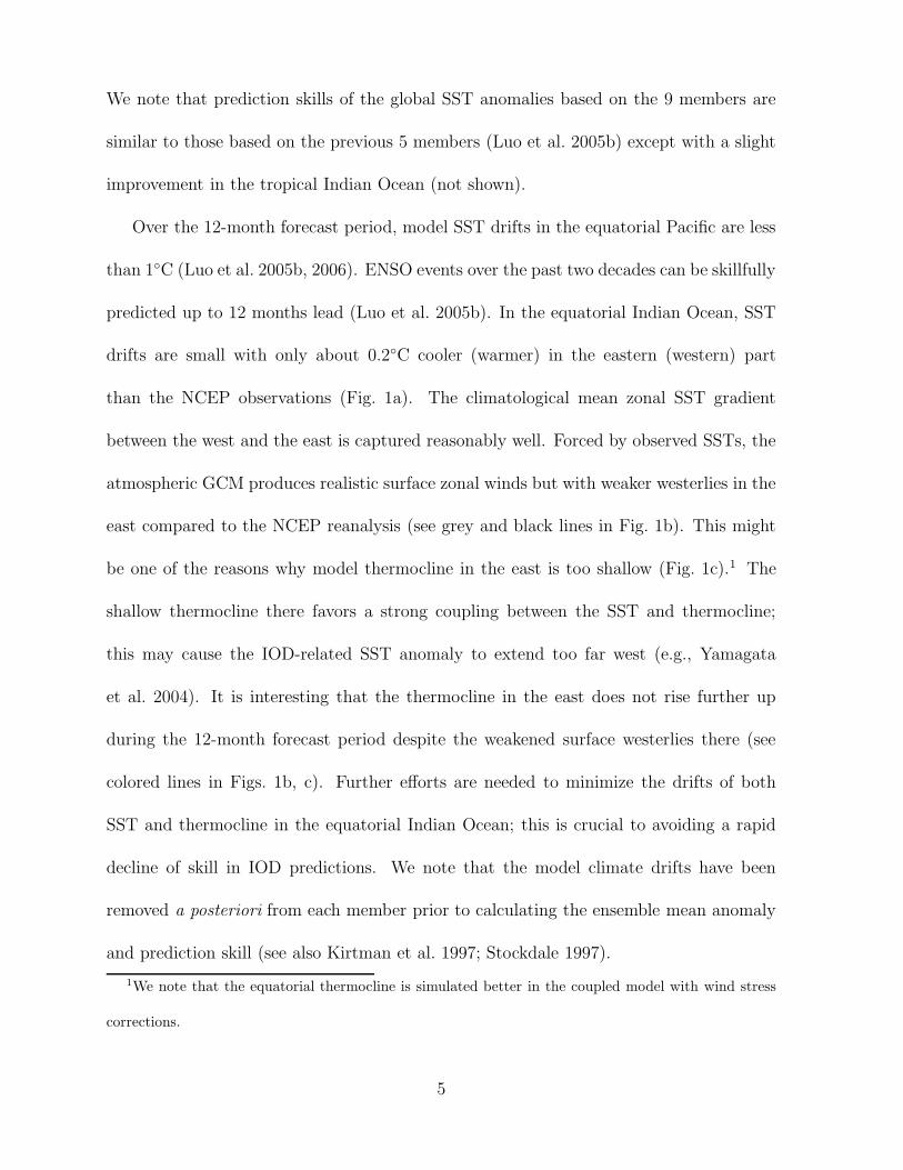
Over the 12-month forecast period, model SST drifts in the equatorial Pacific are less

than 1◦C (Luo et al. 2005b, 2006). ENSO events over the past two decades can be skillfully

predicted up to 12 months lead (Luo et al. 2005b). In the equatorial Indian Ocean, SST

drifts are small with only about 0.2◦C cooler (warmer) in the eastern (western) part

than the NCEP observations (Fig. 1a). The climatological mean zonal SST gradient

between the west and the east is captured reasonably well. Forced by observed SSTs, the

atmospheric GCM produces realistic surface zonal winds but with weaker westerlies in the

east compared to the NCEP reanalysis (see grey and black lines in Fig. 1b). This might

be one of the reasons why model thermocline in the east is too shallow (Fig. 1c).1 The

shallow thermocline there favors a strong coupling between the SST and thermocline;

this may cause the IOD-related SST anomaly to extend too far west (e.g., Yamagata

et al. 2004). It is interesting that the thermocline in the east does not rise further up

during the 12-month forecast period despite the weakened surface westerlies there (see

colored lines in Figs. 1b, c). Further efforts are needed to minimize the drifts of both

SST and thermocline in the equatorial Indian Ocean; this is crucial to avoiding a rapid

decline of skill in IOD predictions. We note that the model climate drifts have been

removed a posteriori from each member prior to calculating the ensemble mean anomaly

and prediction skill (see also Kirtman et al. 1997; Stockdale 1997).

1We note that the equatorial thermocline is simulated better in the coupled model with wind stress

corrections.

5

3. Retrospective forecasts

a. Overall assessment

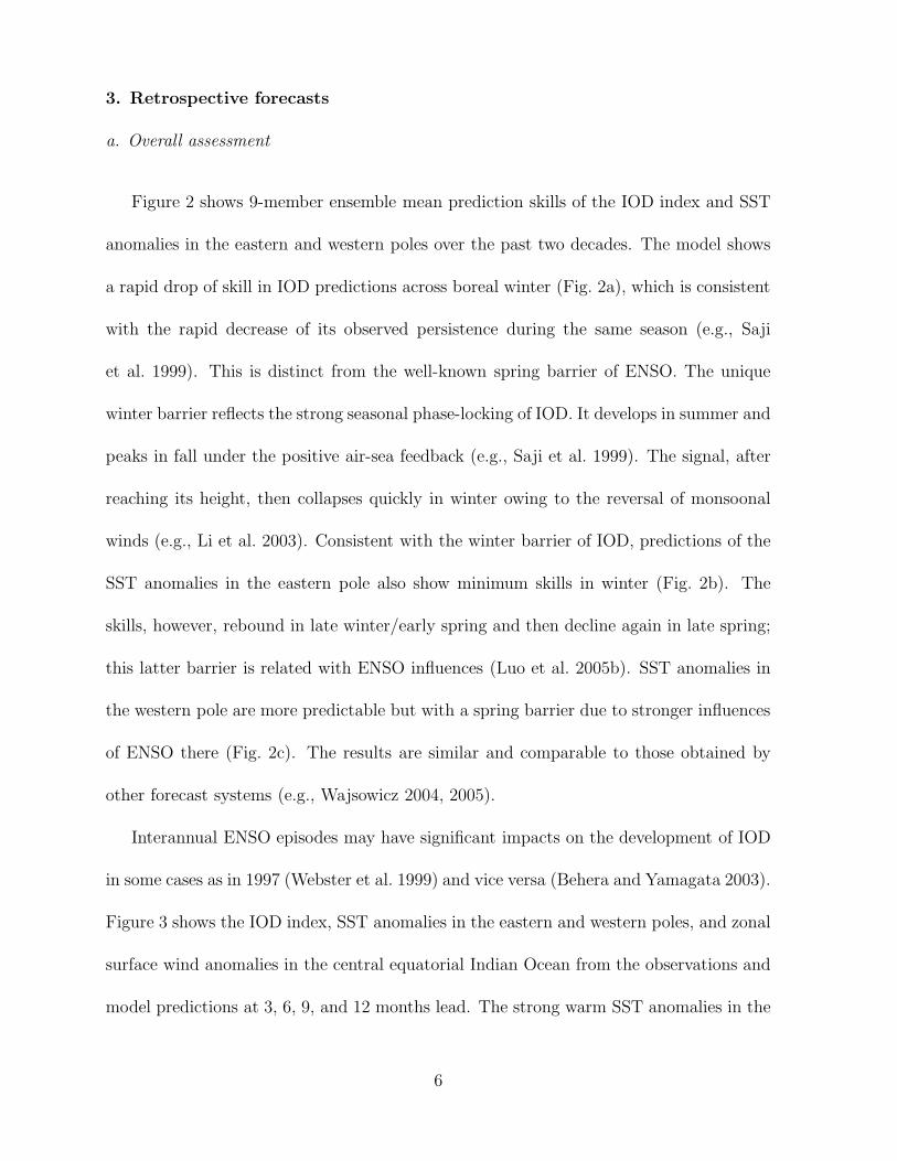
Figure 2 shows 9-member ensemble mean prediction skills of the IOD index and SST

anomalies in the eastern and western poles over the past two decades. The model shows

a rapid drop of skill in IOD predictions across boreal winter (Fig. 2a), which is consistent

with the rapid decrease of its observed persistence during the same season (e.g., Saji

et al. 1999). This is distinct from the well-known spring barrier of ENSO. The unique

winter barrier reflects the strong seasonal phase-locking of IOD. It develops in summer and

peaks in fall under the positive air-sea feedback (e.g., Saji et al. 1999). The signal, after

reaching its height, then collapses quickly in winter owing to the reversal of monsoonal

winds (e.g., Li et al. 2003). Consistent with the winter barrier of IOD, predictions of the

SST anomalies in the eastern pole also show minimum skills in winter (Fig. 2b). The

skills, however, rebound in late winter/early spring and then decline again in late spring;

this latter barrier is related with ENSO influences (Luo et al. 2005b). SST anomalies in

the western pole are more predictable but with a spring barrier due to stronger influences

of ENSO there (Fig. 2c). The results are similar and comparable to those obtained by

other forecast systems (e.g., Wajsowicz 2004, 2005).

Interannual ENSO episodes may have significant impacts on the development of IOD

in some cases as in 1997 (Webster et al. 1999) and vice versa (Behera and Yamagata 2003).

Figure 3 shows the IOD index, SST anomalies in the eastern and western poles, and zonal

surface wind anomalies in the central equatorial Indian Ocean from the observations and

model predictions at 3, 6, 9, and 12 months lead. The strong warm SST anomalies in the

6

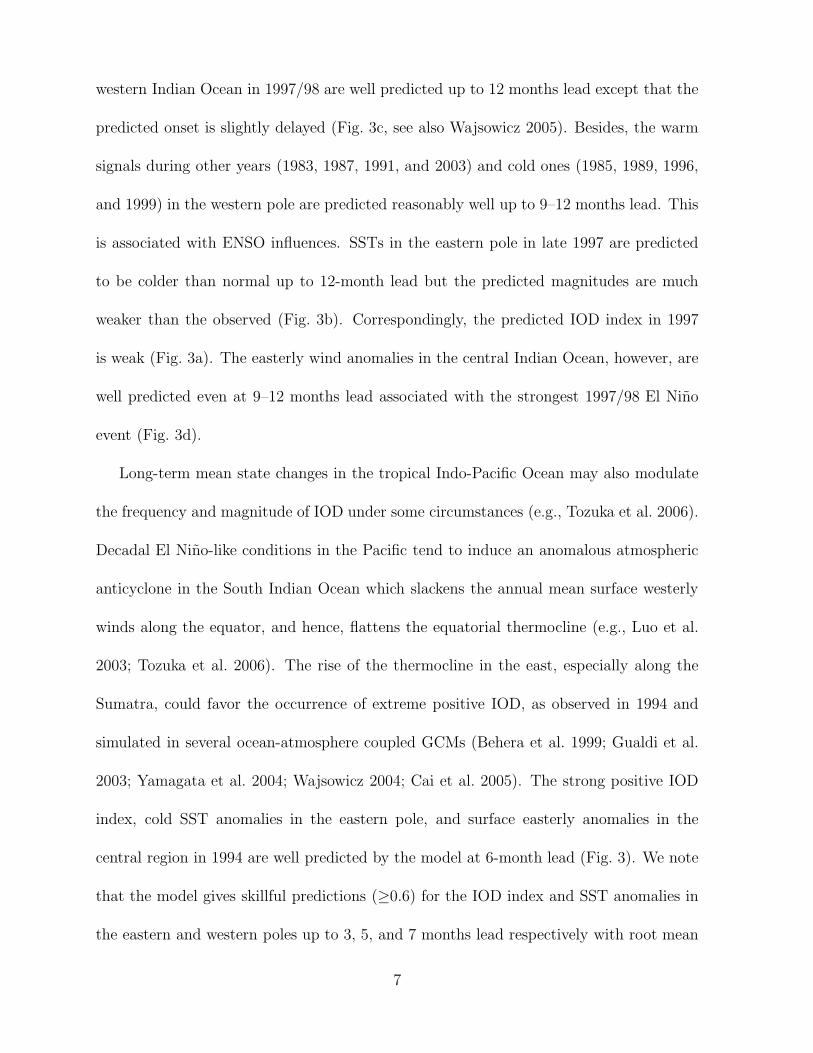
western Indian Ocean in 1997/98 are well predicted up to 12 months lead except that the

predicted onset is slightly delayed (Fig. 3c, see also Wajsowicz 2005). Besides, the warm

signals during other years (1983, 1987, 1991, and 2003) and cold ones (1985, 1989, 1996,

and 1999) in the western pole are predicted reasonably well up to 9–12 months lead. This

is associated with ENSO influences. SSTs in the eastern pole in late 1997 are predicted

to be colder than normal up to 12-month lead but the predicted magnitudes are much

weaker than the observed (Fig. 3b). Correspondingly, the predicted IOD index in 1997

is weak (Fig. 3a). The easterly wind anomalies in the central Indian Ocean, however, are

well predicted even at 9–12 months lead associated with the strongest 1997/98 El Nino

event (Fig. 3d).

Long-term mean state changes in the tropical Indo-Pacific Ocean may also modulate

the frequency and magnitude of IOD under some circumstances (e.g., Tozuka et al. 2006).

Decadal El Nino-like conditions in the Pacific tend to induce an anomalous atmospheric

anticyclone in the South Indian Ocean which slackens the annual mean surface westerly

winds along the equator, and hence, flattens the equatorial thermocline (e.g., Luo et al.

2003; Tozuka et al. 2006). The rise of the thermocline in the east, especially along the

Sumatra, could favor the occurrence of extreme positive IOD, as observed in 1994 and

simulated in several ocean-atmosphere coupled GCMs (Behera et al. 1999; Gualdi et al.

2003; Yamagata et al. 2004; Wajsowicz 2004; Cai et al. 2005). The strong positive IOD

index, cold SST anomalies in the eastern pole, and surface easterly anomalies in the

central region in 1994 are well predicted by the model at 6-month lead (Fig. 3). We note

that the model gives skillful predictions (≥0.6) for the IOD index and SST anomalies in

the eastern and western poles up to 3, 5, and 7 months lead respectively with root mean

7

square errors less than 0.2◦-0.3◦C and a small number of false alarms at these lead times.2

b. Case studies of 1994 and 1997

1) PREDICTION PLUMES

Figure 4 shows the model prediction plumes of the SST anomalies in the two poles of

IOD and in Nino3.4 region during the two extreme positive IOD events of 1994 and 1997.

The cold SST anomalies in the eastern pole during both events can be predicted from

previous fall and winter but with much weakened magnitudes (Fig. 4a). Evolution of the

strong cold SST anomaly in 1994 (i.e., growth in May–July, peak in August–October,

and rapid demise in November–December 1994) is realistically predicted from the spring

of 1994. However, the model fails to predict the 1997 case. This is partly due to the

influence of a warm ISO event in 1997 spring; forecasts initiated from 1 May 1997 even

give a false alarm of a warm condition in 1997 fall (see Fig. 4a). The warm ISO event

is related to an intraseasonal downwelling Kelvin wave generated by the surface westerly

anomalies in the central equatorial Indian Ocean in 1997 spring (e.g., Chambers et al.

1999; Rao and Yamagata 2004). Another shortcoming is that the model could not predict

the strong cold signals in the eastern pole even started from the summer and early fall

of 1997 after the demise of the warm ISO event there. This is related to the errors in

model initial subsurface conditions as shown later. We note that forecast systems with

ocean data assimilation give better predictions for the 1997 event (see Wajsowicz 2004,

2005). In the western Indian Ocean, the strong warm SST anomalies in 1997 are predicted

2Skill scores are reduced by 0.1–0.2 if ISOs are taken into account for calculations. Skillful predictions

of the three unfiltered indices can be made only at 2, 3, and 4 months lead, respectively.

8

reasonably well associated with the well-predicted strong El Nino condition in the Pacific

except that the predicted onsets are slightly delayed (Figs. 4b, c). In contrast, weak and

high-frequency signals appeared in the western pole during 1994; their predictability is

rather low. The model shows a limited predictability for the 1994 mild El Nino-like event

in the Pacific (see also Luo et al. 2005b, 2006).

2) ERROR ANALYSIS

In order to understand the different performance of the model in predicting the eastern

pole SST anomalies between the two IOD events, we have checked the initial thermocline

conditions in 1994 and 1997 (Fig. 5). Oceanic thermocline along the west coast of Sumatra

shallows quickly in 1994 spring associated with strong anomalous southeasterly winds

there (Figs. 5a, c). The 20◦C isotherm is raised to about 10 m above the normal position

during 1994 spring–fall. The model also produces anomalous southeasterly winds in the

eastern region during 1997 but the wind strength is much weaker (Fig. 5c).3 Therefore,

the thermocline in the eastern pole in 1997 has not risen sufficiently enough to provide

favorable initial conditions for the development of strong cold SST anomalies there (Fig.

5b). The thermocline depth anomalies during 1997 spring–fall are much smaller than

those produced by the Simple Ocean Data Assimilation (SODA, Carton et al. 2000).

This suggests that suitable assimilation of the subsurface information could improve the

IOD forecasts. Besides, performance of the atmospheric GCM in simulating the surface

winds in the Indian Ocean needs to be improved.

3) SPATIAL SST AND RAINFALL ANOMALIES

3We note that the southeasterly winds anomaly near the west coast of Sumatra in 1997 is comparable

to that in 1994 according to the NCEP reanalysis.

9

The dipole structure of the SST anomalies (strong colder SSTs in the eastern and

weak warmer ones in the western tropical Indian Ocean) in 1994 boreal fall is successfully

predicted from 1 June 1994 (Figs. 6a, b). The cold SST anomalies (and hence drought),

however, extend far too west to the western equatorial Indian Ocean; this represents

a common model deficiency in simulating the Indian Ocean climate (e.g., Gualdi et al.

2003; Yamagata et al. 2004; Wajsowicz 2004; Cai et al. 2005). Such a bias is related

to a poor simulation of the east-west tilted thermocline in the equatorial Indian Ocean

associated with too weak mean surface westerly winds in the model (see Fig. 1). The

El Nino-like warming in the central equatorial Pacific in 1994 is well predicted but with

weakened magnitudes. The model realistically predicts the drought in the eastern Indian

Ocean, Indonesia, and Australia, and the floods in the western Indian Ocean, South India

and eastern Africa (Figs. 6f, g). The drought along the eastern coast of Asia from the

Indochina Peninsula-Philippines to the western Japan is predicted. Rainfall anomalies

in the Pacific associated with the El Nino-like condition are predicted. Initiated from

1994 spring, the strong cold SST anomalies in the east and the dipole structure of rainfall

anomalies in the Indian Ocean are also predicted realistically (Figs. 6c, h). The similar

features can also be seen in the predictions from 1993/94 winter (Figs. 6d, e, i, j). The

predicted cold SST anomalies near the west coast of Sumatra at the two long-lead times,

however, are much weaker than the observations. Besides, the model gives a false alarm

of a weak cooling in the western Indian Ocean; this is related to the wrongly predicted

La Nina condition in the Pacific (Figs. 6d, e).

The 1997 positive IOD event can be predicted from 1 June 1997 but with much

weakened magnitudes (Figs. 7a, b, f, g). Nevertheless, the dipole pattern of rainfall

10

anomalies in the Indian Ocean and the drought in the Australia and eastern Asia are

predicted reasonably well. The model shows a high predictability of the 1997/98 El Nino

event (Figs. 7c–e). Its related rainfall anomalies in the Pacific (i.e., floods in the central

and eastern equatorial Pacific and drought in the Intertropical Convergence Zone and

South Pacific Convergence Zone) can be predicted from as early as 1996/97 winter (Figs.

7g–j). Correspondingly, warmer SSTs and more rainfall in the western equatorial Indian

Ocean are predicted from the 1996/97 winter and 1997 spring, though the predicted

magnitudes are much weaker than the observations. In contrast, the model predicts weak

cold and even warm SST anomalies along the west coast of Sumatra at these lead times

(Figs. 7c–e). This is due to the fact that anomalous southeasterly winds in the model are

too weak there and hence cannot raise the oceanic thermocline to above the normal level

(see Fig. 5).

4. Experimental real time forecasts

a. Fall and winter in 2005

Our experimental real time forecasts with 18 ensemble members were started in early

2005. To generate 18 initial conditions, we have also used the OI daily SST products

merged from two microwave satellites (TMI and AMSR-E) retrievals available on-line

from June 2002 at http://www.ssmi.com/. One advantage over the infrared satellites is

that the microwave ones are capable of measuring global through-cloud SSTs. We note

that large ensemble members are important to improve the seasonal climate forecasts in

the Indian Ocean due to active ISOs there.

Model forecasts initiated from 1 April to 1 August 2005 showed a weak negative IOD

11

with warm SST anomalies appearing in the eastern Indian Ocean in September–November

2005 and a La Nina condition in the Pacific in 2005/06 winter (Fig. 8). Ensemble spreads

among 18 members are quite large as seen from the forecasts initiated from 1 April

and 1 June 2005; probabilities of both negative and positive IOD events in September–

November 2005 coexist (Fig. 8a). This suggests limited predictability for weak IOD

events. Probabilistic forecasts based on large ensemble members could provide a reliable

solution for this case. We note that ensemble mean forecast tends to have the maximum

likelihood of occurrence if the distribution of ensemble members is not highly irregular

(e.g., Barnston et al. 2005). All ensemble mean forecasts initiated at 1-month intervals

since 1 April 2005 showed a weak negative IOD in 2005 fall; they are consistent with those

initiated from 1 August 2005. The latter have much smaller ensemble spreads.

The weak negative IOD in 2005 fall is primarily caused by the mild warm SST anoma-

lies in the eastern pole; signals in the western pole are very weak (Figs. 8b, c). Corre-

spondingly, predictions for the eastern pole SST anomalies initiated from 1 April and 1

June 2005 also show large ensemble spreads (Fig. 8b). 12 (13) out of the total 18 members

predicted the warmer SSTs there in 2005 fall from 1 April (June) 2005. Success of those

members is related to a deeper thermocline condition near the west coast of Sumatra in

the model (Fig. 9). This again suggests the importance of assimilating subsurface obser-

vations in the prediction system. Realistic subsurface information may help to reduce the

large ensemble spreads and improve the predictability. Despite the nonstrong warming

in the eastern pole, significant floods appeared in 2005 fall due to the warm mean SST

state there (Figs. 10a, c). A clear dipole structure of rainfall anomalies associated with

the negative IOD in 2005 fall was observed. These are predicted reasonably well by the

12

model initiated from 1 June 2005 despite the deficiency that the predicted warm SST

and positive rainfall anomalies extend too far westward (Figs. 10b, d). In the tropical

Pacific, a La Nina condition started to develop in 2005 fall; significant cold SST anomalies

appeared near the west coast of South America (Fig. 10a). This is well predicted by the

model except that the predicted cold signals (and hence drought) extend far too west to

the western and central equatorial Pacific (Figs. 10b, d).

We note that realistic long-range forecast of the La Nina event developed in late

2005 is difficult owing to active ISOs in the equatorial Pacific. Failure in capturing

the strong warm oceanic Kelvin wave during February–May 2005 (because of no assim-

ilation of the subsurface information) leads to the false prediction of an earlier onset

of La Nina (see Fig. 8d). Initial cold subsurface signals were observed in the eastern

Pacific in early August of 2005 and a typical La Nina condition developed in 2005/06

winter (see http://www.cpc.ncep.noaa.gov/products/analysis monitoring/enso update/).

The La Nina condition in 2005/06 winter is successfully predicted from as early as 1 March

2005 by the forecast system (see Figs. 13a, e). However, the rapid decay of the La Nina

signal in 2006 spring is not predicted. Predicting ENSO onset and decay seems to be

rather difficult as found in many other forecast systems (e.g., Landsea and Knaff 2000).

b. Summer and fall in 2006

Figure 11a shows the Indian Ocean subsurface conditions averaged from November

2005 to February 2006 as produced by the coupled SST-nudging scheme. Substantial cold

subsurface signals have appeared in the southwestern Indian Ocean and extended to the

western equatorial region. Such a situation is similar to that in 1993/94 (Fig. 11b) and

13

may favor the development of a positive IOD in the following summer and fall (e.g., Rao et

al. 2002). Besides, newly available observations in the equatorial Pacific up to June 2006

showed that the La Nina signal has finished and warm subsurface signals have appeared in

the east (see http://www.cpc.ncep.noaa.gov/products/analysis monitoring/enso update/).

A warmer condition in the equatorial Pacific might favor the development of a positive

IOD in 2006.

Indeed, the model forecasts initiated since 1 November 2005 consistently show that a

positive IOD would appear in 2006 summer and fall (Fig. 12a). Strong cold SST anomalies

would occur in the eastern pole with weak warm anomalies appearing in the western Indian

Ocean (Figs. 12b, c). The latter is consistent with the model ENSO forecasts (Fig. 12d).

The results show that the La Nina condition in the equatorial Pacific would end in 2006

summer and a weak El Nino might happen if westerly wind bursts in the western Pacific,

which have been active since 2002, would also appear in 2006. We note that the rapid

decay of the La Nina signal in 2006 spring is not well predicted even at short-lead times

(see Fig. 12d).

The consensus forecasts initiated from 1 December 2005 to 1 March 2006 show that

cold SST anomalies would still persist in the central and eastern equatorial Pacific in

2006 spring (Fig. 13b). Correspondingly, warm anomalies would appear in the central

North and South Pacific associated with the atmospheric teleconnections of La Nina. In

the tropical Indian Ocean, basin-wide cold SST anomalies would occur in 2006 spring in

accord with the La Nina condition. These are similar to the newly available observations

except that the observed La Nina condition weakened rather quickly and weak warm

SST anomalies appeared in the equatorial Indian Ocean (Fig. 13f). A clear positive IOD

14

pattern would develop in the following summer and peak in 2006 fall with strong cold

SST anomalies larger than -0.5◦C appearing near the west coast of Sumatra (Figs. 13c,

d). The predicted situation in the tropical Indo-Pacific sector in 2006 summer and fall

seems to be similar to that in 1994.

5. Summary and discussion

In this study, we have investigated the climate predictability in the tropical Indian

Ocean based on 9-member ensemble hindcasts over the past two decades. The results

show skillful scores of the IOD index predictions up to 3-4 months lead with an intrinsic

winter prediction barrier. In the western Indian Ocean, several warm SST anomalies

(during 1983, 1987, 1991, 1997/98, and 2003) and cold anomalies (1985, 1989, 1996, and

1999) can be predicted reasonably well up to 9-12 months lead. This is associated with the

large influences of ENSO which is highly predictable. In contrast, it is rather challenging to

predict the SST anomaly in the eastern Indian Ocean. The model, however, can skillfully

predict the signal there up to about 2 seasons ahead. Considering the complicated and

delicate physical processes governing the IOD and sparse subsurface observations in the

Indian Ocean, it is encouraging that current state-of-the-art ocean-atmosphere coupled

models are capable of predicting the extreme IOD episode in 1994 at 2-3 seasons lead.

It is worth noting that the model fails to predict the strong cold SST anomalies in the

eastern pole in 1997 fall despite the well-predicted strong warming in the western pole

associated with the unprecedented El Nino influence. This is mainly due to the errors in

the initial subsurface conditions associated with too weak southeasterly winds along the

west coast of Sumatra in the model.

15

In the presence of chaotic and energetic ISOs in the Indian Ocean, substantially in-

creasing ensemble members could improve the long-range forecasts of IOD. Large en-

sembles are needed to make reliable probabilistic forecasts. This is a future work. It is

encouraging that the real time forecasts with 18 members realistically predicted the weak

negative IOD in 2005 fall and La Nina condition in 2005/06 winter up to two or three

seasons ahead. Model forecasts initiated since 1 November 2005 show that a positive

IOD event would occur in 2006 summer and fall accompanying with a possible weak El

Nino condition in the equatorial Pacific. We note that such long-lead predictions of IOD,

however, might be reliable only in certain circumstances such as 1994. Model forecasts

should be kept updated on a monthly basis and validated with observations. They are

available online at http://www.jamstec.go.jp/frcgc/research/d1/iod/.

Besides, large efforts are required to improve the performance of both atmospheric and

oceanic GCMs in simulating the tropical Indian Ocean climate. The flat zonal thermocline

in the equatorial Indian Ocean associated with too weak westerly winds in the model

may affect the probability density function of IOD predictions, favoring the occurrence

of strong events. The Indonesia throughflow that carries the water from the western

Pacific to the eastern Indian Ocean must also be resolved in a more precise way in next-

generation coupled models. Errors in the initial subsurface conditions in the tropical

Indian Ocean may largely affect the IOD predictions in some circumstances. Our results

suggest that realistic subsurface information in the eastern Indian Ocean, particularly

along the west coast of Sumatra, could improve the IOD predictions. Besides, strong

subsurface signals in the southwestern tropical Indian Ocean at 5◦S–12◦S can contribute to

the preconditioning of IOD events. Ocean observations with sufficient coverage in this area

16

may help to improve the long-range lead forecasts of IOD. Current international efforts

under WCRP/CLIVAR and EOS/GEOSS/GOOS to establish a long-term monitoring

system in the tropical Indian Ocean (similar to the counterpart TAO/TRITON in the

Pacific) will increase forecast skills of IOD by providing better initial conditions.

Acknowledgments. The SINTEX-F model integrations were carried out on the Earth

Simulator. The atmosphere model (ECHAM4) was provided by MPI-Met, Hamburg;

ocean model (OPA) by LODYC, Paris; and coupler (OASIS) by CERFACS, Toulouse.

We thank Gary Meyers, Antonio Navarra, Stuart Godfrey, Michael McPhaden, Shang-

Ping Xie, and Roxana Wajsowicz for helpful discussions, and two anonymous reviewers

for their valuable comments that helped improving the manuscript greatly.

17

REFERENCES

Ansell, T., C. J. C. Reason, and G. Meyers, 2000: Variability in the tropical southeast

Indian Ocean and links with southeast Australian winter rainfall. Geophys. Res.

Lett., 27, 3977–3980.

Barnston, A. G., A. Kumar, L. Goddard, and M. P. Hoerling, 2005: Improving seasonal

prediction practices through attribution of climate variability. Bull. Amer. Meteor.

Soc., 86, 59–72.

Behera, S., and T. Yamagata, 2003: Influence of the Indian Ocean dipole on the southern

oscillation. J. Meteorol. Soc. Jpn, 81, 169–177.

Behera, S. K., R. Krishnan, and T. Yamagata, 1999: Unusual ocean-atmosphere condi-

tions in the tropical Indian Ocean during 1994. Geophys. Res. Lett., 26, 3001–3004.

Behera, S. K., J.-J. Luo, S. Masson, P. Delecluse, S. Gualdi, A. Navarra, and T. Ya-

magata, 2005: Paramount impact of the Indian Ocean dipole on the East African

short rains: A CGCM study. J. Climate, 18, 4514–4530.

Birkett, C., R. Murtugudde, and T. Allan, 1999: Indian Ocean climate event brings

floods to East Africa’s lakes and the Sudd Marsh. Geophys. Res. Lett., 26, 1031–

1034.

Cai, W., H. H. Hendon, and G. Meyers, 2005: Indian Ocean dipole variability in the

CSIRO mark 3 coupled climate model. J. Climate, 18, 1449–1468.

Cane, M. A., S. E. Zebiak, and S. C. Dolan, 1986: Experimental forecasts of El Nino.

Nature, 321, 827–832.

18

Carton, J. A., G. Chepurin, and X. Cao, 2000: A Simple Ocean Data Assimilation

analysis of the global upper ocean 1950–1995. Part 2: Results. J. Phys. Oceanogr.,

30, 311–326.

Chambers, D. P., B. D. Tapley, and R. H. Stewart, 1999: Anomalous warming in the

Indian Ocean coincident with El Nino. J. Geophys. Res., 104, 3035–3047.

Chen, D., S. E. Zebiak, A. J. Busalacchi, and M. A. Cane, 1995: An improved procedure

for El Nino forecasting: Implications for predictability. Science, 269, 1699–1702.

Clark, C. O., P. J. Webster, and J. E. Cole, 2003: Interdecadal variability of the rela-

tionship between the Indian Ocean Zonal Mode and East African Coastal Rainfall

anomalies. J. Climate, 16, 548–554.

Gualdi, S., E. Guilyardi, A. Navarra, S. Masina, and P. Delecluse, 2003: The interannual

variability in the tropical Indian Ocean as simulated by a CGCM. Climate Dyn.,

10, 567–582.

Han, W., W. T. Liu, and J. Lin, 2006: Impact of atmospheric submonthly oscillations

on sea surface temperature of the tropical Indian Ocean. Geophys. Res. Lett., 33,

L03609, doi:10.1029/2005GL025082.

Kirtman, B. P., J. Shukla, B. Huang, Z. Zhu, and E. K. Schneider, 1997: Multiseasonal

predictions with a coupled tropical ocean-global atmosphere system. Mon. Wea.

Rev., 125, 789–808.

Landsea, C. W., and J. A. Knaff, 2000: How much skill was there in forecasting the very

strong 1997-98 El Nino? Bull. Amer. Meteor. Soc., 81, 2107–2119.

19

Li, T., B. Wang, C.-P. Chang, and Y. Zhang, 2003: A theory for the Indian Ocean

dipole-zonal mode. J. Atmos. Sci., 60, 2119–2135.

Luo, J.-J., S. Masson, S. Behera, and T. Yamagata, 2006: Extended ENSO predictions

using a fully coupled ocean-atmosphere model. J. Climate, submitted.

Luo, J.-J., S. Masson, E. Roeckner, G. Madec, and T. Yamagata, 2005a: Reducing

climatology bias in an ocean-atmosphere CGCM with improved coupling physics.

J. Climate, 18, 2344–2360.

Luo, J.-J., S. Masson, S. Behera, S. Shingu, and T. Yamagata, 2005b: Seasonal cli-

mate predictability in a coupled OAGCM using a different approach for ensemble

forecasts. J. Climate, 18, 4474–4497.

Luo, J.-J., S. Masson, S. Behera, P. Delecluse, S. Gualdi, A. Navarra, and T. Yamagata,

2003: South Pacific origin of the decadal ENSO-like variation as simulated by a

coupled GCM. Geophys. Res. Lett., 30(24), 2250, doi:10.1029/2003GL018649.

Masumoto Y., H. Hase, Y. Kuroda, H. Matsuura, and K. Takeuchi, 2005: Intraseasonal

variability in the upper layer currents observed in the eastern equatorial Indian

Ocean. Geophys. Res. Lett., 32, L02607, doi:10.1029/2004GL021896.

Rao, S. A., and T. Yamagata, 2004: Abrupt termination of Indian Ocean dipole events in

response to intraseasonal disturbances. Geophys. Res. Lett., 31, L19306, doi:10.1029

/2004GL020842.

Rao, S. A., S. Behera, Y. Masumoto, and T. Yamagata, 2002: Interannual variability

in the subsurface Indian Ocean with special emphasis on the Indian Ocean Dipole.

20

Deep Sea Res., 49, 1549–1572.

Saji, N. H., and T. Yamagata, 2003: Interference of teleconnection patterns generated

from the tropical Indian and Pacific Oceans. Climate Res., 25, 151–169.

Saji, N. H., B. N. Goswami, P. N. Vinayachandran, and T. Yamagata, 1999: A dipole

mode in the tropical Indian ocean. Nature, 401, 360–363.

Stockdale, T. N., 1997: Coupled ocean-atmosphere forecasts in the presence of climate

drift. Mon. Wea. Rev., 125, 809–818.

Stockdale, T. N., D. L. T. Anderson, J. O. S. Alves, and M. A. Balmaseda, 1998: Global

seasonal rainfall forecasts using a coupled ocean-atmosphere model. Nature, 392,

370–373.

Tozuka, T., J.-J. Luo, S. Masson, and T. Yamagata, 2006: Decadal modulations of the

Indian Ocean Dipole in the SINTEX-F1 coupled GCM. J. Climate, in press.

Yamagata, T., S. Behera, J.-J. Luo, S. Masson, M. Jury, and S. A. Rao, 2004: Coupled

ocean-atmosphere variability in the tropical Indian Ocean. Earth’s Climate: The

Ocean-Atmosphere Interaction. Geophys. Monogr., 147, Amer. Geophys. Union,

189–212.

Wajsowicz, R. C., 2004: Climate variability over the tropical Indian Ocean sector in the

NSIPP seasonal forecast system. J. Climate, 17, 4783–4804.

Wajsowicz, R. C., 2005: Potential predictability of tropical Indian Ocean SST anomalies.

Geophys. Res. Lett., 32, L24702, doi:10.1029/2005GL024169.

21

Webster, P. J., A. Moore, J. Loschnigg, and M. Leban, 1999: Coupled ocean-atmosphere

dynamics in the Indian Ocean during 1997-98. Nature, 401, 356–360.

22

Figure captions

Fig. 1: a) Annual mean SST climatology of the period 1983–2004 in the equatorial

Indian Ocean (2◦S–2◦N) based on the NCEP observations (black line), 9-member mean

forecasts at 3, 6, 9, and 12 months lead (red, green, blue, and yellow lines). b) Same as

in a), but for the surface zonal winds at 10 m height. Grey line denotes 9-member mean

values produced by the coupled SST-nudging scheme. c) Same as in b), but for the 20◦C

isotherm depth. Black line denotes the World Ocean Atlas 2001 observations.

Fig. 2: Seasonally stratified anomaly correlation coefficients (ACC) between the obser-

vations and model predictions during 1982–2004 for a) the IOD index, b) SST anomalies

in the eastern pole (EIO, 90◦–110◦E, 10◦S–0◦), and c) the western pole (WIO, 50◦–70◦E,

10◦S–10◦N). Contour interval is 0.1 and regions with values above 0.6 are shaded. The

IOD index is defined as the SST anomaly difference between the western and eastern

pole. Skills are calculated based on the time series of 5-month running mean of both the

observations and model hindcasts at each lead time. This tends to give proper estimates

of the predictability of climate variations beyond the intraseasonal timescale (Luo et al.

2005b).

Fig. 3: (a–d) IOD index, EIO and WIO SST anomalies, and surface zonal wind

anomaly in the central equatorial Indian Ocean (Ueq, 70◦–90◦E, 5◦S–5◦N) based on the

NCEP observations (black lines) and model predictions at 3, 6, 9, and 12 months lead

(red, green, blue, and yellow lines). Results have been smoothed with 5-month running

mean. We note that, despite the model weak climatology, interannual Ueq variations

produced by the coupled SST-nudging scheme (see grey line in d) are similar to the

23

NCEP reanalysis.

Fig. 4: Left (right) panels: Predictions of the monthly EIO, WIO, and Nino3.4 (5◦S–

5◦N, 170◦–120◦W) SST anomalies initiated from 1 September, and 1 November 1993

(1996), 1 January, 1 May, and 1 September 1994 (1997) (red, blue, grey, yellow, and

green lines). The thick solid black and colored curves denote the NCEP monthly analysis

and 9-member ensemble mean forecasts respectively. The dashed lines show each member

forecasts. Results are based on unfiltered data.

Fig. 5: EIO 20◦C isotherm depth anomalies in a) 1994 and b) 1997 produced by

the coupled SST-nudging scheme for individual members (short-dashed lines) and en-

semble mean (thick solid lines). SODA reanalysis (thick dashed lines) is also shown

for comparison. c) Model surface wind differences between March–September 1997 and

March–September 1994.

Fig. 6: (a–e) SST anomalies averaged in September–November 1994 based on the

observations and model 9-member ensemble mean predictions from 1 December 1993, and

1 February, 1 April, and 1 June 1994 respectively. Contour interval 0.3◦C and regions

with negative values are shaded. (f–j) As in (a–e), but for the precipitation anomalies

(contour: 0, ±0.5, ±1, ±3, ±5 mm day−1...). Results have been spatially smoothed with

nearby 9 points for clarity.

Fig. 7: Same as in Fig. 6, but for the period of September-November 1997.

Fig. 8: (a–d) Forecasts of the monthly IOD index, EIO, WIO, and Nino3.4 SST

anomalies initiated from 1 April, 1 June, and 1 August 2005 respectively. The blue

curves denote NCEP monthly analysis and the red curves the 18-member ensemble mean

forecasts for 12 target months.

24

Fig. 9: Differences of the model 20◦C isotherm depth anomalies (contour: 3 m) in

April and June 2005. These are based on two groups of members which predicted warmer

and colder SSTs in the eastern pole in 2005 fall.

Fig. 10: Same as in Fig. 6, but for the 2005 fall SST and precipitation anomalies based

on the observations and model predictions from 1 June 2005.

Fig. 11: 20◦C isotherm depth anomalies (contour: 5 m) averaged a) from November

2005 to February 2006 and b) from November 1993 to February 1994. These are produced

by the coupled SST-nudging scheme based on the NCEP SST observations.

Fig. 12: Same as in Fig. 8, but for the model forecasts initiated from 1 November, and

1 December 2005, 1 January, 1 February, and 1 March 2006 respectively. We note that

recent predictions from 1 April, 1 May, and 1 June 2006 also show a positive IOD in 2006

summer and fall (see http://www.jamstec.go.jp/frcgc/research/d1/iod/).

Fig. 13: a) SST anomalies of December 2005–February 2006 predicted from 1 March

2005. (b–d) Predicted SST anomalies during March–May, June–August, and September–

November 2006. These are produced by the average of four recent 18-member mean

forecasts initiated from 1 December 2005, 1 January, 1 February, and 1 March 2006

respectively. Observed SST anomalies in 2005/06 winter and 2006 spring are also shown

in e) and f). Contour interval 0.3◦C and regions with negative values are shaded.

25

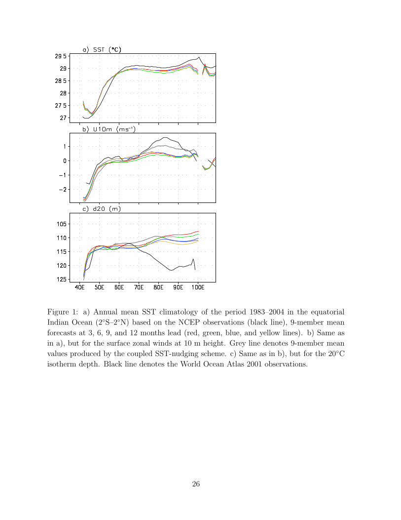
Figure 1: a) Annual mean SST climatology of the period 1983–2004 in the equatorial

Indian Ocean (2◦S–2◦N) based on the NCEP observations (black line), 9-member mean

forecasts at 3, 6, 9, and 12 months lead (red, green, blue, and yellow lines). b) Same as

in a), but for the surface zonal winds at 10 m height. Grey line denotes 9-member mean

values produced by the coupled SST-nudging scheme. c) Same as in b), but for the 20◦C

isotherm depth. Black line denotes the World Ocean Atlas 2001 observations.

26

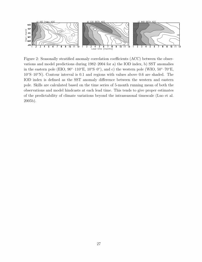
Figure 2: Seasonally stratified anomaly correlation coefficients (ACC) between the obser-

vations and model predictions during 1982–2004 for a) the IOD index, b) SST anomalies

in the eastern pole (EIO, 90◦–110◦E, 10◦S–0◦), and c) the western pole (WIO, 50◦–70◦E,

10◦S–10◦N). Contour interval is 0.1 and regions with values above 0.6 are shaded. The

IOD index is defined as the SST anomaly difference between the western and eastern

pole. Skills are calculated based on the time series of 5-month running mean of both the

observations and model hindcasts at each lead time. This tends to give proper estimates

of the predictability of climate variations beyond the intraseasonal timescale (Luo et al.

2005b).

27

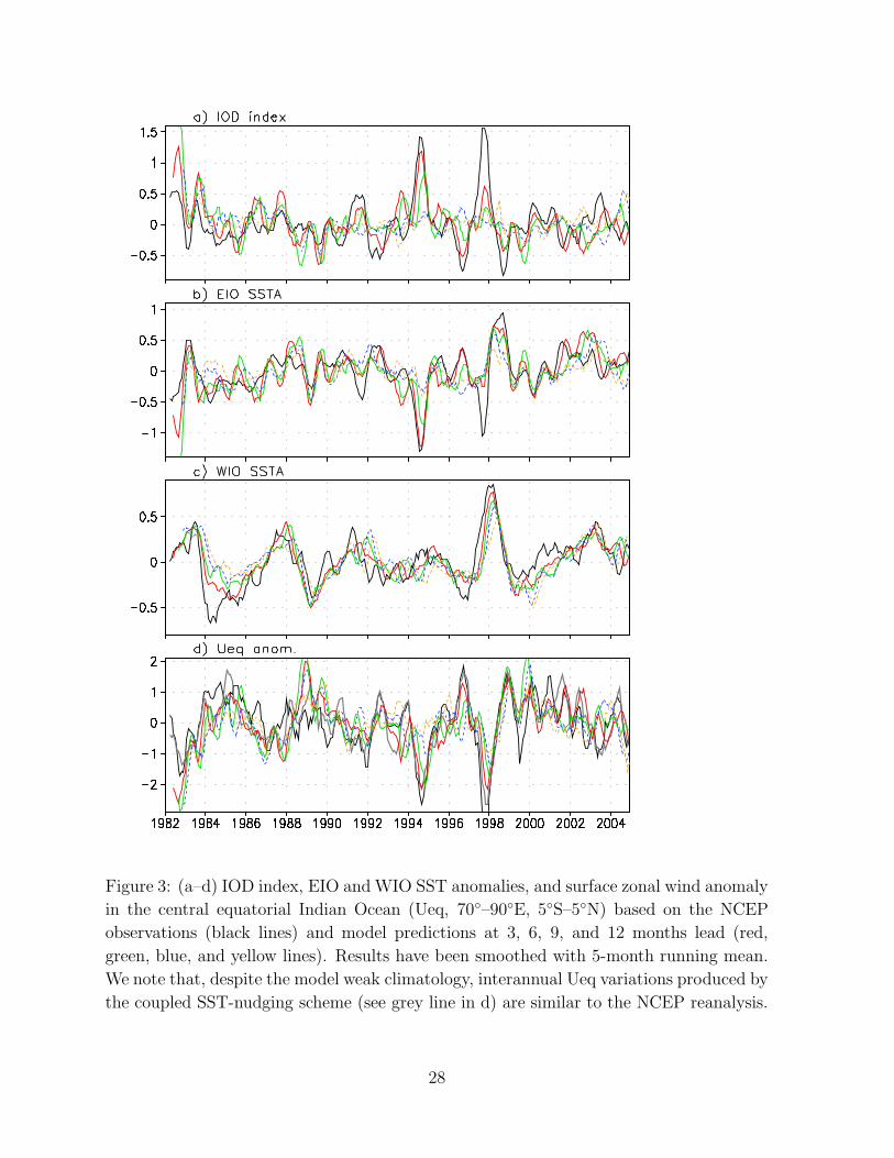
Figure 3: (a–d) IOD index, EIO and WIO SST anomalies, and surface zonal wind anomaly

in the central equatorial Indian Ocean (Ueq, 70◦–90◦E, 5◦S–5◦N) based on the NCEP

observations (black lines) and model predictions at 3, 6, 9, and 12 months lead (red,

green, blue, and yellow lines). Results have been smoothed with 5-month running mean.

We note that, despite the model weak climatology, interannual Ueq variations produced by

the coupled SST-nudging scheme (see grey line in d) are similar to the NCEP reanalysis.

28

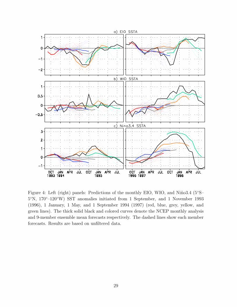
Figure 4: Left (right) panels: Predictions of the monthly EIO, WIO, and Nino3.4 (5◦S–

5◦N, 170◦–120◦W) SST anomalies initiated from 1 September, and 1 November 1993

(1996), 1 January, 1 May, and 1 September 1994 (1997) (red, blue, grey, yellow, and

green lines). The thick solid black and colored curves denote the NCEP monthly analysis

and 9-member ensemble mean forecasts respectively. The dashed lines show each member

forecasts. Results are based on unfiltered data.

29

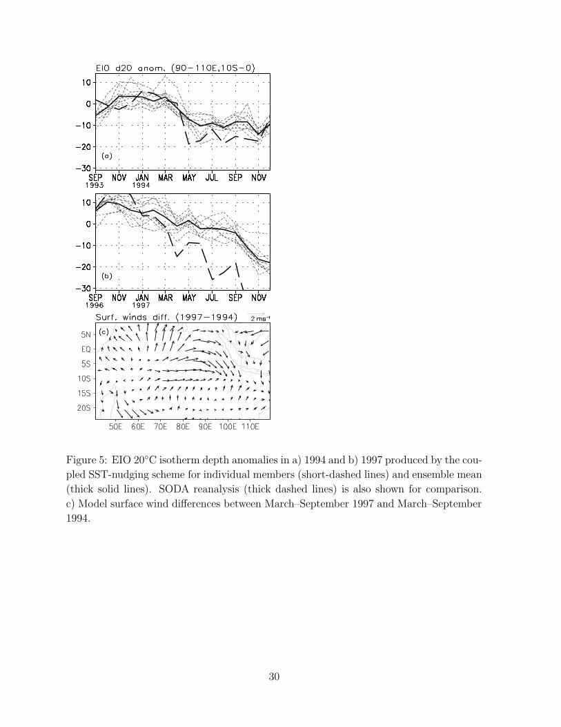
Figure 5: EIO 20◦C isotherm depth anomalies in a) 1994 and b) 1997 produced by the cou-

pled SST-nudging scheme for individual members (short-dashed lines) and ensemble mean

(thick solid lines). SODA reanalysis (thick dashed lines) is also shown for comparison.

c) Model surface wind differences between March–September 1997 and March–September

1994.

30

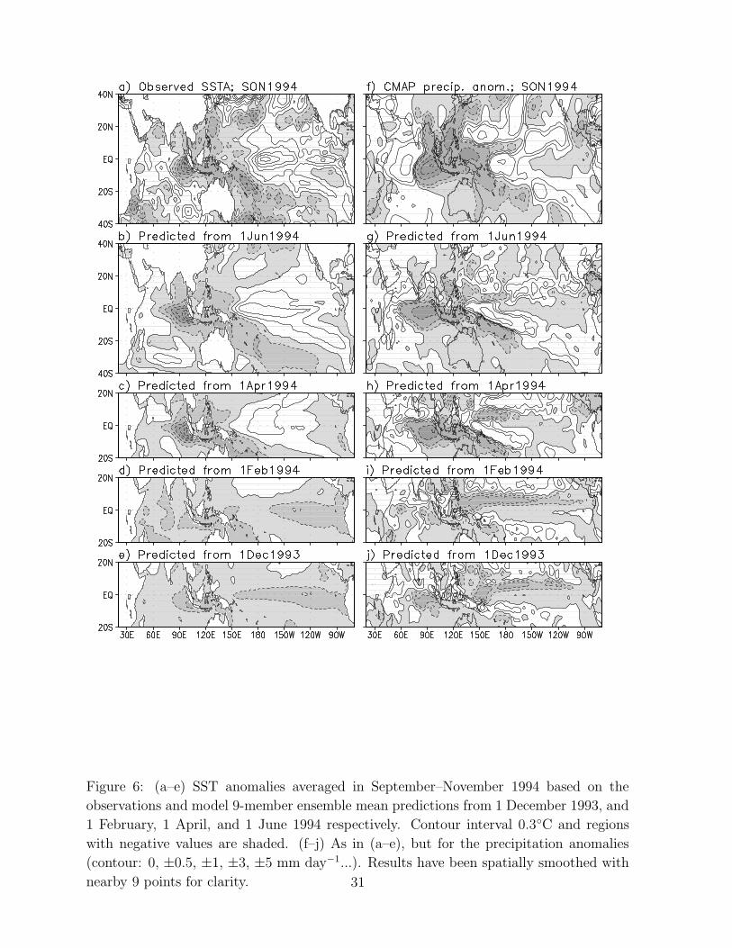
Figure 6: (a–e) SST anomalies averaged in September–November 1994 based on the

observations and model 9-member ensemble mean predictions from 1 December 1993, and

1 February, 1 April, and 1 June 1994 respectively. Contour interval 0.3◦C and regions

with negative values are shaded. (f–j) As in (a–e), but for the precipitation anomalies

(contour: 0, ±0.5, ±1, ±3, ±5 mm day−1...). Results have been spatially smoothed with

nearby 9 points for clarity. 31

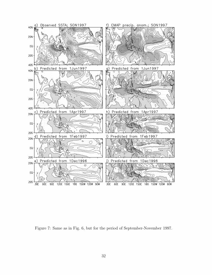
Figure 7: Same as in Fig. 6, but for the period of September-November 1997.

32

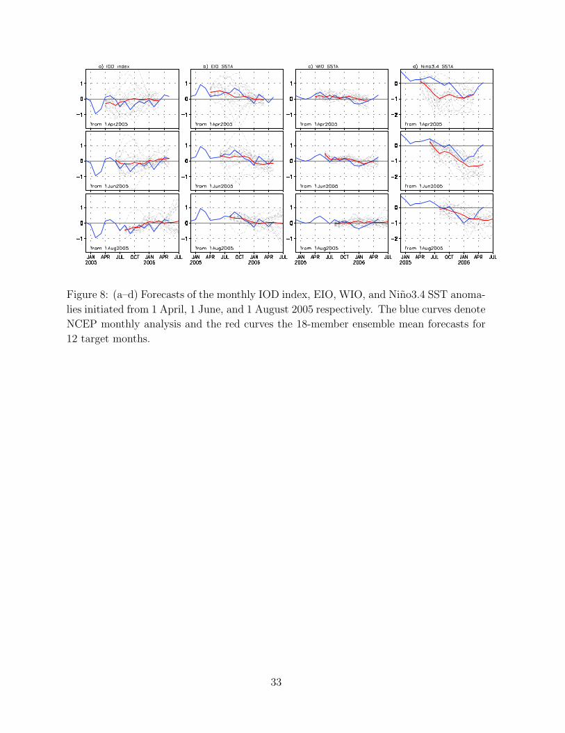
Figure 8: (a–d) Forecasts of the monthly IOD index, EIO, WIO, and Nino3.4 SST anoma-

lies initiated from 1 April, 1 June, and 1 August 2005 respectively. The blue curves denote

NCEP monthly analysis and the red curves the 18-member ensemble mean forecasts for

12 target months.

33

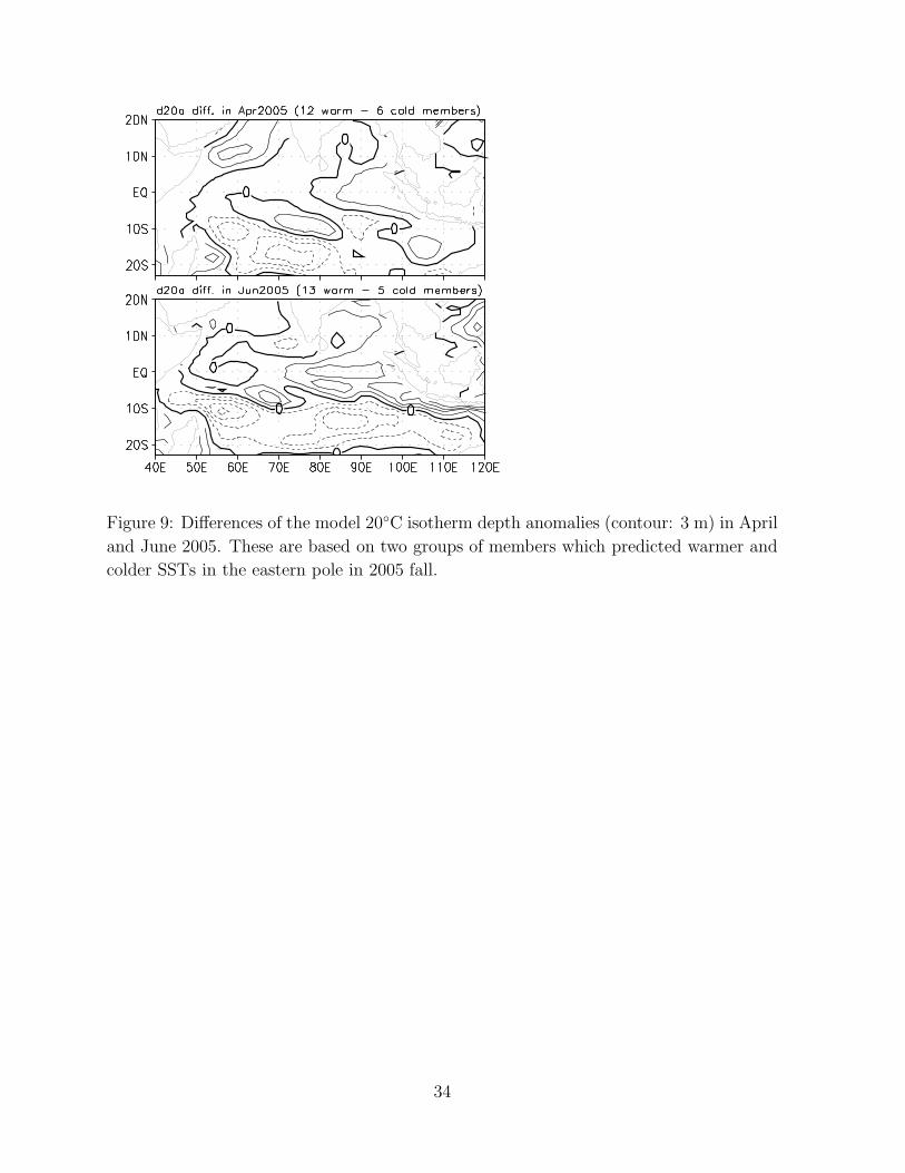
Figure 9: Differences of the model 20◦C isotherm depth anomalies (contour: 3 m) in April

and June 2005. These are based on two groups of members which predicted warmer and

colder SSTs in the eastern pole in 2005 fall.

34

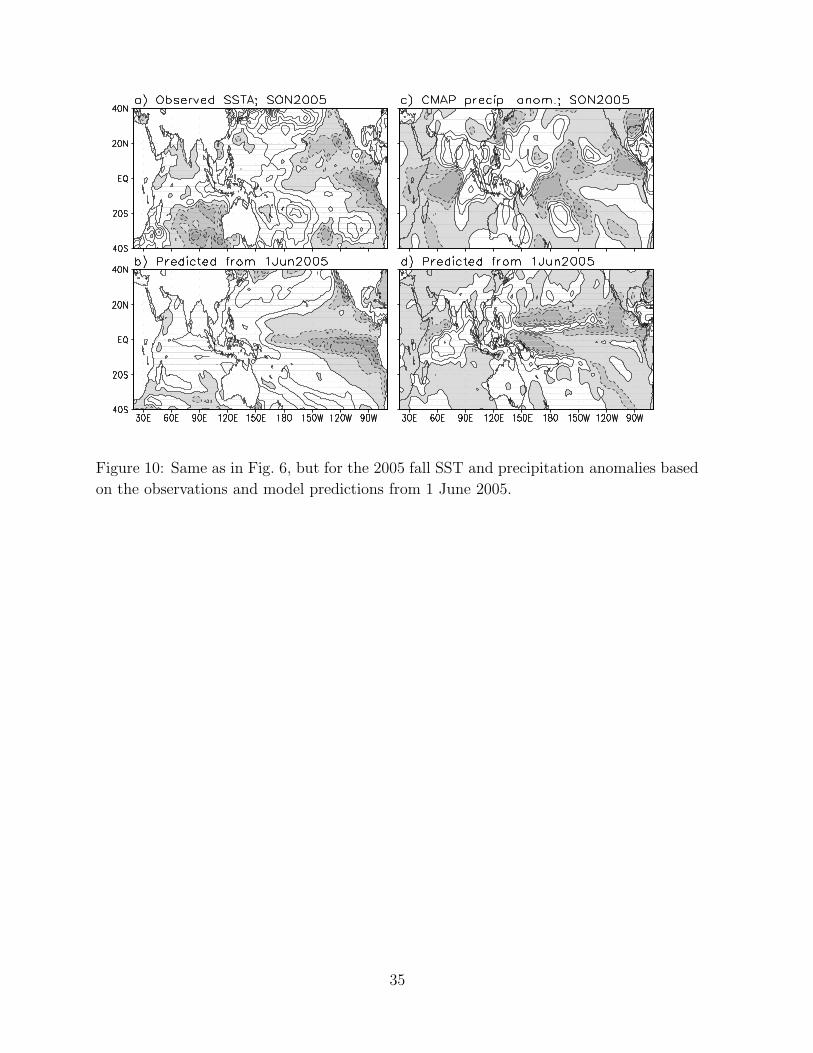
Figure 10: Same as in Fig. 6, but for the 2005 fall SST and precipitation anomalies based

on the observations and model predictions from 1 June 2005.

35

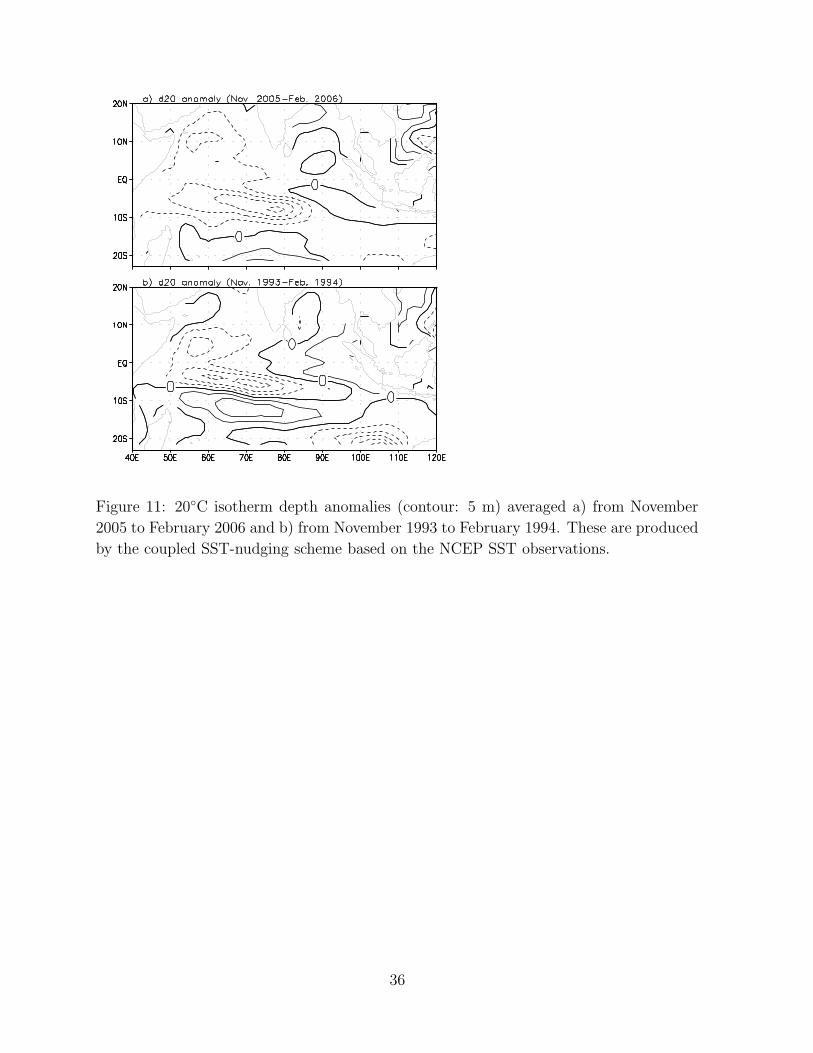
Figure 11: 20◦C isotherm depth anomalies (contour: 5 m) averaged a) from November

2005 to February 2006 and b) from November 1993 to February 1994. These are produced

by the coupled SST-nudging scheme based on the NCEP SST observations.

36

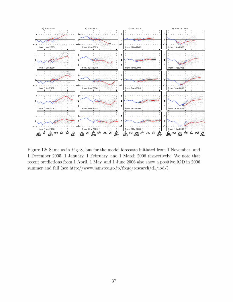
Figure 12: Same as in Fig. 8, but for the model forecasts initiated from 1 November, and

1 December 2005, 1 January, 1 February, and 1 March 2006 respectively. We note that

recent predictions from 1 April, 1 May, and 1 June 2006 also show a positive IOD in 2006

summer and fall (see http://www.jamstec.go.jp/frcgc/research/d1/iod/).

37

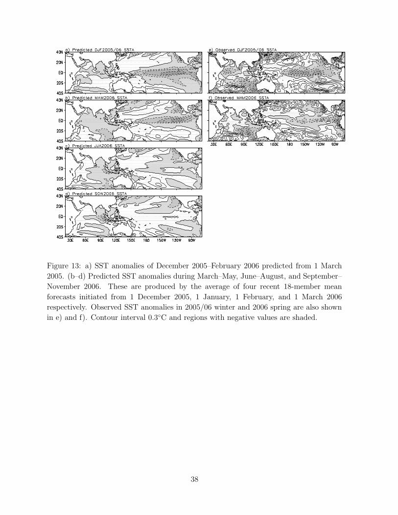
Figure 13: a) SST anomalies of December 2005–February 2006 predicted from 1 March

2005. (b–d) Predicted SST anomalies during March–May, June–August, and September–

November 2006. These are produced by the average of four recent 18-member mean

forecasts initiated from 1 December 2005, 1 January, 1 February, and 1 March 2006

respectively. Observed SST anomalies in 2005/06 winter and 2006 spring are also shown

in e) and f). Contour interval 0.3◦C and regions with negative values are shaded.

38