Experimental identification of effective masstransport models in falling film flows

P. Bandi†, S. Gro߇, M. Karalashvili∗, A. Mhamdi∗, H. Pirnay∗, L. Zhang‡,W. Marquardt∗, M. Modigell†, A. Reusken‡

In many industrial units (e.g. packing columns, falling film reactors), the liq-uid phase is designed as a falling film, since it is well known that the mass andheat transfer in laminar-wavy film flows is significantly enhanced. Computationaldesign models which account for these enhanced transport mechanisms are nec-essary. The numerical simulation of the coupled momentum and mass transportequations is computationally infeasible due to its multiphase nature and the dy-namic, unstable interface. To overcome this problem, we propose a transportmodel based on effective diffusion coefficients and suggest an incremental approachfor its identification. This incremental approach is computationally feasible whilestill accounting for the wave-induced transport intensification. The model identi-fication is based on high-resolution concentration measurements of oxygen beingphysically absorbed into an aqueous film applying a planar laser-induced lumines-cence (pLIL) measurement technique. Preliminary measurement and estimationresults are presented.

Keywords. Falling film, mass transport, effective diffusion coefficient, incremental identi-fication, concentration measurements, numerical simulation.

1 Introduction

In industrial applications such as CO2 scrubbers, falling film evaporators, absorption heatpumps as well as many others, falling films are widely used. In these devices the liquid phaseoccurs as a gravity driven thin film. The heat and mass transport properties in these filmsare significantly intensified by their waviness [4]. The dynamic and complex structure of thefilm complicate its detailed experimental and numerical analysis. Therefore, falling films aresubject to ongoing research efforts (see [9, 17, 22, 23, 27] and the references therein). Despitethese efforts, the understanding of the transport phenomena is still limited and comprehensivetransport models are not available.

The direct numerical treatment of first principle models for mass transport inside thefilm require the simultaneous solution of the two-phase Navier-Stokes equations of the gasand liquid phase. In available simulations, unphysical effects are often observed, leadingto the conclusion that today’s numerical tools are not mature enough to be relied upon.

∗Process Systems Engineering, RWTH Aachen, Germany†Mechanical Process Engineering, RWTH Aachen, Germany‡Chair for Numerical Mathematics, RWTH Aachen, Germany

1

These observations show that there is a need for reduced design models, which are capable ofmodeling the defining properties of the transport phenomena in falling films while keepingthe computational demand down to a minimum.

In this work, a transport model for liquid falling films based on effective diffusion coeffi-cients is proposed. The model will be identified using incremental model-based identification.This approach calls for a close collaboration between experiments, numerics and modeling.Examples for this collaboration are the development of stabilization methods in the inverseproblems of the identification and the application of model-based image processing to theexperimental data.

By combining these complementary expertises, a versatile systematic toolbox is created. Inthis paper we describe the main ideas underlying our interdisciplinary approach fo derivingan effective mass transport model in falling film flows.

The paper is organized as follows. First, the modeling approach is described in detail,focusing on the derivation of the reduced model. This is followed by an explanation of thenumerical methods employed, focusing on stabilization for convection-dominated problems,as well as the solution of PDEs on wavy computational domains. The pLIL measurementtechnique, as well as the experimental setup is introduced in the third part. First results ofthe joint work are presented.

2 Incremental Modeling and Identification

In this section, a transport model for liquid falling films based on effective diffusion coeffi-cients is proposed. First, the reduced flow model used for the convection-diffusion equationsemerging in these problems is described. Then, the model structure is derived using theincremental method. For the subsequent model identification, the incremental method is em-ployed. Finally, the solution of the inverse problems appearing in the model identification isoutlined.

2.1 One-phase wavy film model

As described above, the direct numerical simulation of the Navier-Stokes equations for thetwo-phase flow model of the liquid and gas phase is currently infeasible and even in the longerrun impractical in an industrial environment. Therefore, the detailed two-phase flow model isreplaced by a reduced one-phase flow model of the liquid phase. The film height δ(x, z, t) ofthe wavy film is computed from an evolution equation based on the Long-Wave theory. Weemploy a two-equation expansion of the film thickness δ and the volume flow rate V in thefilm. These expansions have been shown to accurately describe the film for a wide range offlow regimes [21].

The velocity profile u inside the film is computed from V , by assuming a parabolic velocityprofile. The three parameters of this parabolic profile are determined by the mass balance,no-slip condition at the wall, and vanishing shear-stress at the free boundary. Note that asopposed to the flat-film solution (Nusselt solution) of the film profile used in previous studies[14], the flow conditions defined by δ and u do not necessarily satisfy the Navier-Stokesequations. However, they are an easily obtainable, reasonable approximation and yield amore accurate description of the state of the film.

2

Using the film height δ, the time-dependent computational domain Ωf (t) is defined as

Ωf (t) = (x, y, z) ∈ R3 | 0 < y < δ(x, z, t), x ∈ (0, Lx), z ∈ (0, Lz) . (1)

All PDEs introduced in the following sections will be defined on the set Ωf (t).

2.2 Incremental Modeling

In order to achieve transparency in the modeling procedure, the incremental method as de-scribed by [19, 20] is applied. Starting point for the incremental procedure is the generictransient balance equation

ct +∇ · J = 0, (2)

where J is the overall molecular flux and ct is the derivative of the concentration w.r.t. time.J can be separated into a convective term induced by the velocity field u and a diffusive termJD,

J = cu + JD. (3)

Using (2) and the fact that ∇ · u = 0 for incompressible fluids, this leads to

ct + u · ∇c+∇ · JD = 0. (4)

Note that in this modeling step the diffusion term JD is not yet specified. The decision on amodel for JD follows in the next step. We assume a flux according to Fick’s law

JD = −Deff∇c, (5)

where Deff is the unknown, state dependent diffusion coefficient. This diffusion coefficient isfurther divided into the contribution of the molecular diffusion Dmol and effects due to thewaviness of the film Dw,

Deff = Dmol +Dw. (6)

The molecular diffusion Dmol is constant and known from the literature. The wavy diffusioncoefficient Dw is unknown, and is introduced to describe the enhancement of mass transportdue to the waviness in the film. On the final level of detail in the modeling process, a modelfor Dw is specified. As nothing is known a priori of the wavy diffusion coefficient, we postulatea general model

Dw(x, y) = fw (c, x, t, θ) (7)

with model parameters θ ∈ Rn.The procedure outlined above for the incremental modeling of mass transfer can be applied

in the same way to the problem of heat transfer in the falling film [14]. The boundaryconditions, however, are different for every experimental setup. The conditions used in ourstudy of transport of oxygen from the gas into the liquid phase are as follows. In our setup(cf. Figure 3), we set a Dirichlet condition for the concentration at the inlet boundary Γin.The value of this concentration is taken from measurements of the inlet chamber. The surfaceboundary Γsurf is modeled as a Dirichlet boundary, as well. We assume that the limitingprocess is the transport within the liquid phase. Therefore, the concentration at the boundaryis set to the equilibrium concentration corresponding to the concentration in the gas phase.The remaining boundaries are modeled using zero-flux Neumann conditions. The location ofthe boundaries is illustrated in Figure 3.

3

2.3 Incremental Identification

The structure and parameters of the function fw introduced in (7) are identified using themethod of incremental identification. The identification closely follows the steps of the in-cremental modeling procedure. In a first step, the generic diffusive flux JD is identified. Tomake this problem numerically more tractable, we introduce a source term Feff = −∇ · JD =∇ · (Dmol∇c) + Fw, yielding

ct + u · ∇c = Feff . (8)

For reasons of numerical stability, the molecular diffusion is included into the left-hand sideof the equation,

ct + u · ∇c−∇ · (Dmol∇c) = Fw, (9)

with Fw representing the divergence of the wavy part of JD. Given the high resolutiondistributed concentration measurements cm obtained in the experiments, the source term Fw

is identified. In a second step, the wavy diffusion coefficient is inferred from the definition ofthe source term

−∇ · (Dw∇c) = −Fw. (10)

Note that the source term only accounts for the enhanced diffusion induced by Dw, as themolecular diffusion was included to convert (8) into a parabolic PDE. An important feature ofthis equation is the fact that the time does not appear explicitly. After Dw and thus Deff hasbeen identified from (10), the model structure fw can be identified using finite-dimensionalnonlinear optimization methods.

The full modeling and identification procedure is illustrated in Figure 1. The model identifi-cation approach described here has several advantages over the method of direct identificationof the parameters θ from the full model

ct + u · ∇c−∇ · ((Dmol + fw(θ))∇c) = 0. (11)

One of the main challenges of this full model identification problem is that the structureof the model fw is completely unknown. To identify the correct structure, the full-scalenonlinear instationary problem (11) would have to be solved for each model candidate. Inthe incremental approach presented above, the parameters of the model are only identified inthe final step. This means that the time consuming step of discriminating among a large setof candidate models does not have to be done in the context of an inverse PDE problem, butinstead in the much simpler framework of function approximation.

2.4 Solution of the inverse problems

In the incremental method described above, a series of consecutive inverse problems has tobe solved. As the balance equations for heat and mass transfer are very similar, we use thesame methods here as in previous studies on the identification of heat transfer in wavy films[15, 16].

4

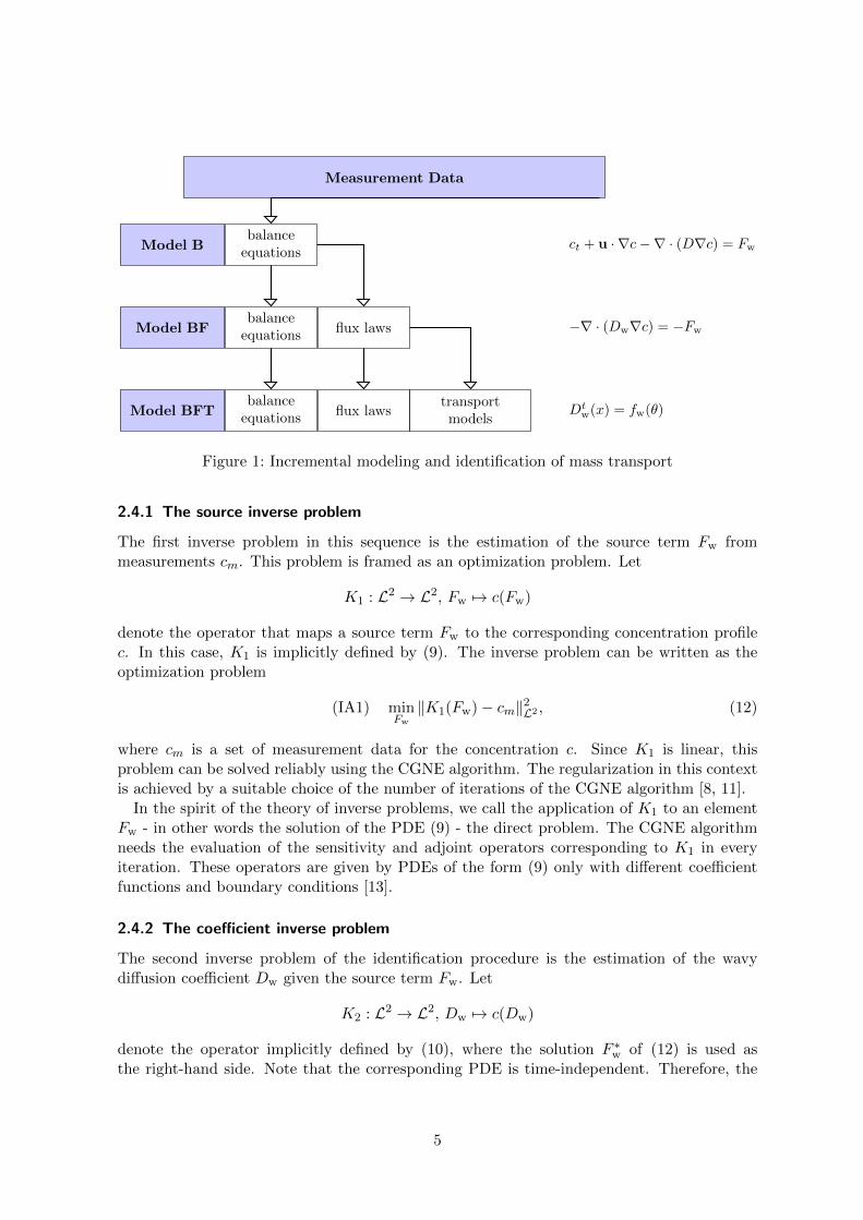
Measurement Data

Model B

Model BF

Model BFT

balanceequations

balanceequations

balanceequations

flux laws

flux lawstransportmodels

ct + u · ∇c−∇ · (D∇c) = Fw

−∇ · (Dw∇c) = −Fw

Dtw(x) = fw(θ)

Figure 1: Incremental modeling and identification of mass transport

2.4.1 The source inverse problem

The first inverse problem in this sequence is the estimation of the source term Fw frommeasurements cm. This problem is framed as an optimization problem. Let

K1 : L2 → L2, Fw 7→ c(Fw)

denote the operator that maps a source term Fw to the corresponding concentration profilec. In this case, K1 is implicitly defined by (9). The inverse problem can be written as theoptimization problem

(IA1) minFw

‖K1(Fw)− cm‖2L2 , (12)

where cm is a set of measurement data for the concentration c. Since K1 is linear, thisproblem can be solved reliably using the CGNE algorithm. The regularization in this contextis achieved by a suitable choice of the number of iterations of the CGNE algorithm [8, 11].

In the spirit of the theory of inverse problems, we call the application of K1 to an elementFw - in other words the solution of the PDE (9) - the direct problem. The CGNE algorithmneeds the evaluation of the sensitivity and adjoint operators corresponding to K1 in everyiteration. These operators are given by PDEs of the form (9) only with different coefficientfunctions and boundary conditions [13].

2.4.2 The coefficient inverse problem

The second inverse problem of the identification procedure is the estimation of the wavydiffusion coefficient Dw given the source term Fw. Let

K2 : L2 → L2, Dw 7→ c(Dw)

denote the operator implicitly defined by (10), where the solution F ∗w of (12) is used asthe right-hand side. Note that the corresponding PDE is time-independent. Therefore, the

5

solutions to different time steps can be decoupled and the problem is solved for each timestep independently.

After the decoupling of the time steps, nt problems of the type

(IA2) minDtw‖K2(Dt

w)− ctm‖2L2 (13)

need to be solved, where nt is the number of time steps, ctm denotes the concentration mea-surement data at time t and the superscript t indicates the value of a function at time t. Forthese nonlinear inverse problems, we use the truncated Newton CG algorithm described in[11].

2.4.3 Correction step and parametric model identification

One drawback of the incremental method is that errors introduced in one identification steppropagate directly into all following steps. In (IA2), Dw is estimated using the solution F ∗wof the previous source-inverse problem. Any error introduced in F ∗w will therefore influencethe solution D∗w as well. To damp this propagation of error, a so-called correction stepis performed to reconcile the solution with the measurements. The correction step is thesolution of the inverse problem

(IA12) minDw

‖K12(Dw)− cm‖2L2 (14)

where K12 is implicitly defined by the PDE

ct + u · ∇c−∇ · ((Dmol +Dw)∇c) = 0 (15)

with the usual boundary conditions. It is important to note that this is much easier afterhaving solved (IA2), since the uncorrected solutions Dw of (IA2) serve as good initial valuesfor the Newton-CG algorithm.

After the wavy coefficient has been found, a parametric model Dw = fw(θ) is identified.This is again done through an optimization problem minimizing the mismatch between themodel fw and data Dw. This problem can be framed in the form of a nonlinear optimizationproblem

minθ‖Di

w − f(ci, xi, ti, θ)‖2. (16)

by regarding the value Diw each grid point i at which Dw is available as a data point.

3 Numerical Simulation

Concerning the numerical simulation tool used in this project we distinguish two classesof methods. Firstly, for the identification steps described in Section 2, sufficiently accuratesolutions to the PDEs representing the direct, sensitivity, and adjoint sensitivity operators areneeded. Secondly, as a long-term goal the simulation of the fully three-dimensional two-phaseflow model can be used as input (simulated, artificial data) for the identification procedure.If the full-scale simulation can achieve a good agreement with the experimental data, thesesimulations could serve as an valuable source of high resolution measurements. This secondgoal, however, is beyond the scope of this paper and will not be further addressed here.

6

All direct, sensitivity, and adjoint problems are of either elliptic or parabolic (convection-diffusion) type. Hence, similar numerical techniques can be employed for their solution. Tothis end, we employed the FEM code DROPS [7, 10]. DROPS is based on multilevel nestedgrids and conforming finite element discretization methods (FEM). For time discretization,a standard one-step θ-method is used. For the space discretization, piecewise linear finiteelements on a tetrahedral grid are employed. The resulting discrete systems of linear equa-tions are solved by suitable Krylov subspace methods. In case of the convection-diffusionequations, we use a preconditioned generalized minimal residuals (GMRES) method [24]. Forthe diffusion problems, a preconditioned CG method is applied.

In the following, we will address two specific issues that are important for an efficientincremental identification algorithm.

3.1 Stabilization of convection-dominated problems

Consider the convection-diffusion equation (9) with the source term Fw(x, t) which is thedirect problem in (IA1) above. The molecular diffusion parameter Dmol = O(10−9)m2/s is

relatively small in our applications. For falling film problems, the ratio‖u‖2Dmol

is of the order

O(107 v 108). Even if we use very fine grids, with mesh size denoted by h, the Peclet number

Pe =h‖u‖22Dmol

is still much larger than 1. It is well-known that for standard FEM in convection-dominated problems oscillations may appear at boundary layers due to the lack of upwindingin standard FEM. The outflow boundary condition at Γout does not cause a boundary layer inthe solution, but a boundary layer may appear at the wavy free surface. Besides that, in theadjoint problem for (IA1) the flow direction is reversed which means that we have Dirichletboundary conditions at the outflow Γin. In this case numerical oscillations are observed ifsuitable stabilization techniques are not employed.

Furthermore, in a strongly convection-dominated problem iterative solvers are often slow,because the resulting linear systems have matrices with large condition numbers and eigen-values with large imaginary parts. Introducing a stabilization in the discretization helps toreduce numerical oscillations and to improve relevant matrix properties.

Among the various stabilization techniques for FEM, we choose the streamline upwindPetrov-Galerkin (SUPG) method [5], which has been implemented in DROPS. This led to asignificant decrease in computation times for convection dominated problems. In addition, areduction of oscillations for the adjoint problem was observed.

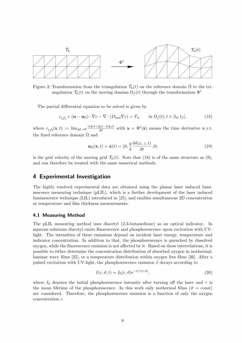
3.2 Arbitrary Lagrangian-Eulerian techniques for free surface

To handle the time-dependent domain Ωf (t) defined in (1) we use an Arbitrary Lagrangian-Eulerian approach (ALE) [3, 6, 18]. We assume that the local time-dependent film thicknessδ(x, z, t) is a known quantity which has been calculated based on the Long-Wave Theory,cf. Section 2.1. Let Ω be a fixed reference domain and Φ : Ω × (0, T ) → Rd a deformationfunction such that (cf. Fig. 2)

Ωf (t) = x = Φt(x) := Φ(x, t) : x ∈ Ω for all t ∈ (0, T ). (17)

Due to the fact that the height of the free surface is an a-priori known function δ(x, z, t), thedeformation of grids can therefore be achieved by a simple transformation of the y-coordinate.

7

Φt

Th Th(t)

Figure 2: Transformation from the triangulation Th(t) on the reference domain Ω to the tri-angulation Th(t) on the moving domian Ωf (t) through the transformation Φt

The partial differential equation to be solved is given by

ct,Ω + (u− uΩ) · ∇c−∇ · (Dmol∇c) = Fw in Ωf (t), t ∈ [t0, tf ], (18)

where ct,Ω(x, t) := lim∆t→0c(x,t+∆t)−c(x,t)

∆t with x = Φt(x) means the time derivative w.r.t.

the fixed reference domain Ω and

uΩ(x, t) = x(t) = (0,y

δ

∂δ(x, z, t)

∂t, 0) (19)

is the grid velocity of the moving grid Th(t). Note that (18) is of the same structure as (9),and can therefore be treated with the same numerical methods.

4 Experimental Investigation

The highly resolved experimental data are obtained using the planar laser induced lumi-nescence measuring technique (pLIL), which is a further development of the laser inducedluminescence technique (LIL) introduced in [25], and enables simultaneous 2D concentrationor temperature and film thickness measurements.

4.1 Measuring Method

The pLIL measuring method uses diacetyl (2,3-butanedione) as an optical indicator. Inaqueous solutions diacetyl emits fluorescence and phosphorescence upon excitation with UV-light. The intensities of these emissions depend on incident laser energy, temperature andindicator concentration. In addition to that, the phosphorescence is quenched by dissolvedoxygen, while the fluorescence emission is not affected by it. Based on these interrelations, it ispossible to either determine the concentration distribution of absorbed oxygen in isothermal,laminar wavy films [25], or a temperature distribution within oxygen free films [26]. After apulsed excitation with UV-light, the phosphorescence emission I decays according to

I(c, ϑ, t) = I0(c, ϑ)e−t/τ(c,ϑ), (20)

where I0 denotes the initial phosphorescence intensity after turning off the laser and τ isthe mean lifetime of the phosphorescence. In this work only isothermal films (ϑ = const)are considered. Therefore, the phosphorescence emission is a function of only the oxygenconcentration c.

8

The dissolved oxygen acts as a physical quencher and reduces not only the lifetime, butalso the initial intensity of the phosphoresence. This correlation is given by the Stern-Volmerequation

τ

τ0=I0

I∗0=

1

1 + c/ch. (21)

In this equation I∗0 and τ0 are the initial intensity and the mean lifetime of the phosphorescencein an oxygen-free solution. I0 and τ relate to the same quantities according to the oxygenconcentration in the system. The parameter ch is the half-value concentration.

Combination of (20) and (21) yields a formulation of the phosphorescence decay as afunction of the local oxygen concentration,

I

I∗0=

τ

τ0e−

tτ . (22)

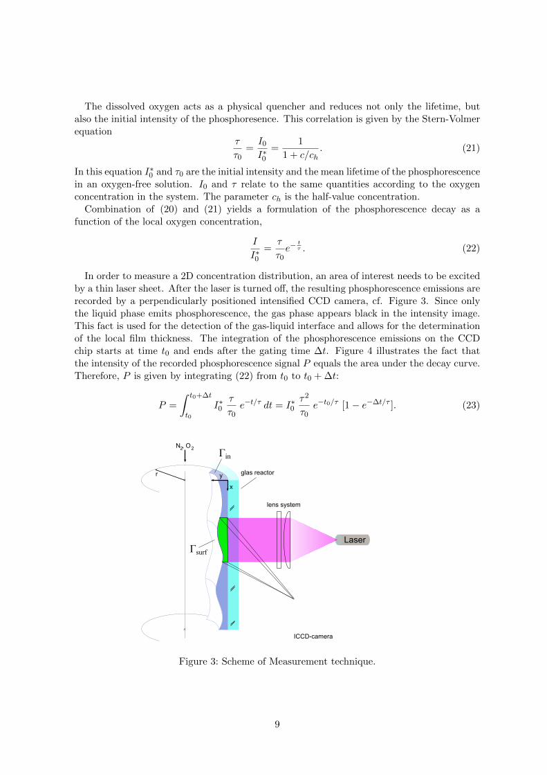
In order to measure a 2D concentration distribution, an area of interest needs to be excitedby a thin laser sheet. After the laser is turned off, the resulting phosphorescence emissions arerecorded by a perpendicularly positioned intensified CCD camera, cf. Figure 3. Since onlythe liquid phase emits phosphorescence, the gas phase appears black in the intensity image.This fact is used for the detection of the gas-liquid interface and allows for the determinationof the local film thickness. The integration of the phosphorescence emissions on the CCDchip starts at time t0 and ends after the gating time ∆t. Figure 4 illustrates the fact thatthe intensity of the recorded phosphorescence signal P equals the area under the decay curve.Therefore, P is given by integrating (22) from t0 to t0 + ∆t:

P =

∫ t0+∆t

t0

I∗0τ

τ0e−t/τ dt = I∗0

τ2

τ0e−t0/τ [1− e−∆t/τ ]. (23)

glas reactory

x

r

N , O 2 2

lens system

ICCD-camera

LaserΓsurf

Γin

Figure 3: Scheme of Measurement technique.

9

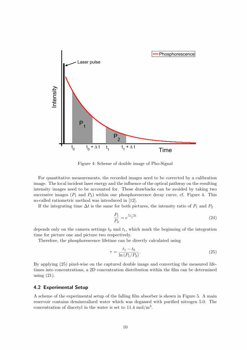
Time

Inte

nsity

Phosphorescence

Laser pulse

t0 + Δ tt0 t1 t1 + Δ t

P1

P2

Figure 4: Scheme of double image of Pho-Signal

For quantitative measurements, the recorded images need to be corrected by a calibrationimage. The local incident laser energy and the influence of the optical pathway on the resultingintensity images need to be accounted for. These drawbacks can be avoided by taking twosuccessive images (P1 and P2) within one phosphorescence decay curve, cf. Figure 4. Thisso-called ratiometric method was introduced in [12].

If the integrating time ∆t is the same for both pictures, the intensity ratio of P1 and P2

P1

P2= e

t1−t0τ (24)

depends only on the camera settings t0 und t1, which mark the beginning of the integrationtime for picture one and picture two respectively.

Therefore, the phosphorescence lifetime can be directly calculated using

τ =t1 − t0

ln (P1/P2). (25)

By applying (25) pixel-wise on the captured double image and converting the measured life-times into concentrations, a 2D concentration distribution within the film can be determinedusing (21).

4.2 Experimental Setup

A scheme of the experimental setup of the falling film absorber is shown in Figure 5. A mainreservoir contains demineralized water which was degassed with purified nitrogen 5.0. Theconcentration of diacetyl in the water is set to 11.4 mol/m3.

10

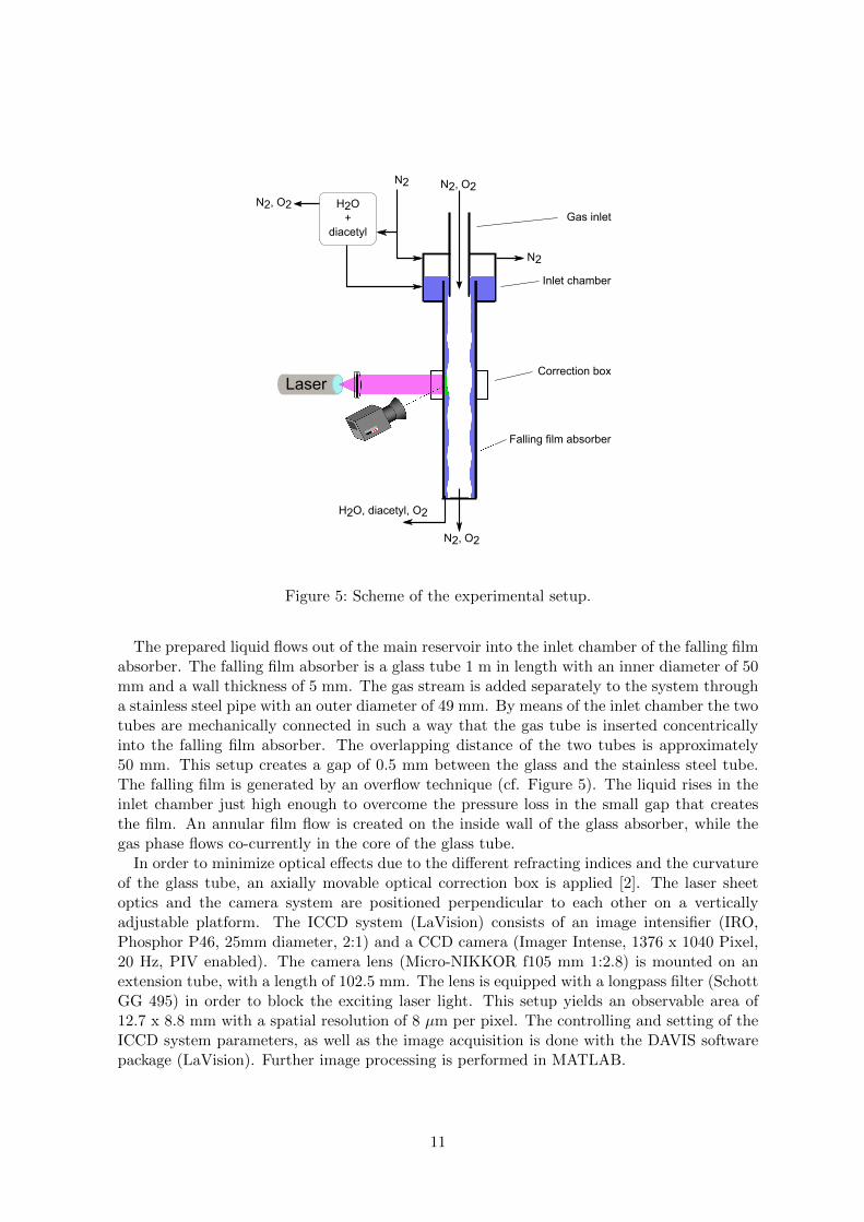
N2, O2

N2, O2

H2O+

diacetyl

H2O, diacetyl, O2

N2

N2, O2

LaserCorrection box

Falling film absorber

Inlet chamber

Gas inlet

N2

Figure 5: Scheme of the experimental setup.

The prepared liquid flows out of the main reservoir into the inlet chamber of the falling filmabsorber. The falling film absorber is a glass tube 1 m in length with an inner diameter of 50mm and a wall thickness of 5 mm. The gas stream is added separately to the system througha stainless steel pipe with an outer diameter of 49 mm. By means of the inlet chamber the twotubes are mechanically connected in such a way that the gas tube is inserted concentricallyinto the falling film absorber. The overlapping distance of the two tubes is approximately50 mm. This setup creates a gap of 0.5 mm between the glass and the stainless steel tube.The falling film is generated by an overflow technique (cf. Figure 5). The liquid rises in theinlet chamber just high enough to overcome the pressure loss in the small gap that createsthe film. An annular film flow is created on the inside wall of the glass absorber, while thegas phase flows co-currently in the core of the glass tube.

In order to minimize optical effects due to the different refracting indices and the curvatureof the glass tube, an axially movable optical correction box is applied [2]. The laser sheetoptics and the camera system are positioned perpendicular to each other on a verticallyadjustable platform. The ICCD system (LaVision) consists of an image intensifier (IRO,Phosphor P46, 25mm diameter, 2:1) and a CCD camera (Imager Intense, 1376 x 1040 Pixel,20 Hz, PIV enabled). The camera lens (Micro-NIKKOR f105 mm 1:2.8) is mounted on anextension tube, with a length of 102.5 mm. The lens is equipped with a longpass filter (SchottGG 495) in order to block the exciting laser light. This setup yields an observable area of12.7 x 8.8 mm with a spatial resolution of 8 µm per pixel. The controlling and setting of theICCD system parameters, as well as the image acquisition is done with the DAVIS softwarepackage (LaVision). Further image processing is performed in MATLAB.

11

Parameter Symbol Value Unit

kinematic viscosity ν 1.0 mm2/smolecular diffusion coefficient Dmol 0.002 mm2/sinitial concentration c0 10 kmol/mm3

liquid volume flow V 8 l/h

Table 1: Fluid properties used in the simulation

A nitrogen pumped laser is used as an excitation light source (LTB Berlin). At a pulsewidth of 700 ps each pulse has an energy of 116 µJ. The maximum repetition rate is 50Hz. By using a 4,4 - diphenylstilbene dye (Radiant Laser Dyes) in a laser cuevette, theoriginal nitrogen laser wavelength is shifted from 337 nm to 405 nm, at which diacetyl has anabsorption maximum.

Currently, flow regimes in the range of Re = 5 - 50 can be investigated. The waviness ofthe falling film is induced by external vibrations. The mixing and setting of the volume fluxof the gas phase is performed using two mass flow controller (ANALYT-MTC) and allows foran accurate adjustment of the gas phase composition.

5 Results

In this section, results on the model identification (with simulated data) and the experimentalmethod are presented.

5.1 Model identification

We present first results for the source inverse problem (12). To illustrate the suitability ofthe proposed numerical method, it is applied to a simulated data set.

For the computational domain Ωf defined by the film surface δ, the Nusselt flat film solutionwas used. For the fluid properties, we assumed water with the properties defined in Table 1.

The length lx of the computational domain in flow direction is set to 100mm. Since theflow properties of the film are constant in z-direction, the choice of the width lz = 1mm isarbitrary. The film height δ is set to the Nusselt height of the film, given by

δ =

(3 Vl ν

g

)1/3

. (26)

The velocity field is zero in all but the x-direction. For the x-direction, it takes on theparabolic form

u(y) = uN

(2y

ly−(y

ly

)2)

(27)

with the Nusselt velocity uN defined as

uN =g δ2

2 ν. (28)

12

0

5 · 10−2

0.10

4 · 10−4−10

0

10

·10−3

xy 0 5 · 10−2 0.1

−1

−0.5

0

0.5

1·10−2

x

Fsol

Fsim

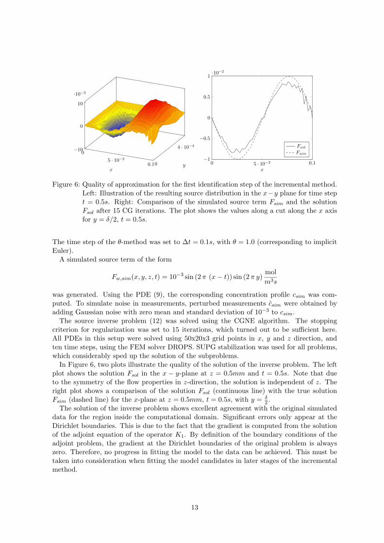
Figure 6: Quality of approximation for the first identification step of the incremental method.Left: Illustration of the resulting source distribution in the x−y plane for time stept = 0.5s. Right: Comparison of the simulated source term Fsim and the solutionFsol after 15 CG iterations. The plot shows the values along a cut along the x axisfor y = δ/2, t = 0.5s.

The time step of the θ-method was set to ∆t = 0.1s, with θ = 1.0 (corresponding to implicitEuler).

A simulated source term of the form

Fw,sim(x, y, z, t) = 10−3 sin (2π (x− t)) sin (2π y)mol

m3s

was generated. Using the PDE (9), the corresponding concentration profile csim was com-puted. To simulate noise in measurements, perturbed measurements csim were obtained byadding Gaussian noise with zero mean and standard deviation of 10−3 to csim.

The source inverse problem (12) was solved using the CGNE algorithm. The stoppingcriterion for regularization was set to 15 iterations, which turned out to be sufficient here.All PDEs in this setup were solved using 50x20x3 grid points in x, y and z direction, andten time steps, using the FEM solver DROPS. SUPG stabilization was used for all problems,which considerably sped up the solution of the subproblems.

In Figure 6, two plots illustrate the quality of the solution of the inverse problem. The leftplot shows the solution Fsol in the x − y-plane at z = 0.5mm and t = 0.5s. Note that dueto the symmetry of the flow properties in z-direction, the solution is independent of z. Theright plot shows a comparison of the solution Fsol (continuous line) with the true solutionFsim (dashed line) for the x-plane at z = 0.5mm, t = 0.5s, with y = δ

2 .The solution of the inverse problem shows excellent agreement with the original simulated

data for the region inside the computational domain. Significant errors only appear at theDirichlet boundaries. This is due to the fact that the gradient is computed from the solutionof the adjoint equation of the operator K1. By definition of the boundary conditions of theadjoint problem, the gradient at the Dirichlet boundaries of the original problem is alwayszero. Therefore, no progress in fitting the model to the data can be achieved. This must betaken into consideration when fitting the model candidates in later stages of the incrementalmethod.

13

Table 2: Parameters of the experimental setup

Parameter Name Value

Liquid flow Reynolds number / - Rel 16Gas flow Reynolds number / - Reg 82

Liquid flow rate / l h−1 Vl 8

Gas flow rate / l h−1 Vg 180Environmental temperature / C ϑ 25.7Phosphorescence lifetime / µs τ0 214Intensifier gain / % Gain 90Intensifier gating time / µs ∆t 200Time between laser pulse and and start of image acquisition / µs t0 8Time delay between start of each image acquisition / µs t1 - t0 230

5.2 Experimental results

The experimental settings are summarized in Table 2. The images were taken 150 mmafter the inlet. Prior to the actual experiments, reference images were taken to correct thedistortions caused by the curvature of the glass tube. For the recording of these correctionimages, the falling film absorber was flooded with the water-diacetyl solution. A referenceplate with a regular pattern on it was submerged into it, placed at the position of interest,and photographed. In a pre-editing image processing step, the built-in calibration routine ofthe camera software used these reference recordings to correct the images. Simultaneously,this correction procedure provided the required scale.

The low intensity of the phosphorescence emission requires a high gain setting for the im-age intensifier. This reduces the obtainable signal to noise ratio and therefore the spatialresolution. At the current development stage of the experimental setup, the images do showquantitatively if oxygen is present in the gas phase. Nevertheless, it is not possible to de-termine concentration distributions accurately within the film. However, with the currentexperimental setup, film thickness measurements are feasible. In the following only oxygen-free falling films are taken into account.

In Figure 5.2, a double image is shown as an example. Both images show the same wave,recorded successively during one decay curve within 430 µs. The red lines depict the gas/liquidinterface and the position of the wall. While the position of the glass wall can be easilydetected automatically, the gas/liquid interface needs to be marked manually. The halo,which can be seen above the film surface, hinders an automated surface detection. This effectis caused by scattered light originating from the excited volume. Since the excited diacetylmolecules emit light in all directions, and the light rays travel from an optical denser into a anoptical thinner material, they are diffracted at the film surface away from the axis of incidence.This results in a phantom image of the wave, which appears as a halo [1]. In addition to that,the physical phenomenon of total reflection accounts for a second optical effect, which canbe seen in the images. Within the wave, a non-constant intensity distribution is observed,even though no oxygen is present in the film and diacetyl is homogeneously distributed in theliquid. At the gas/liquid interface the intensity distribution reaches its maximum and the filmsurface is identifiable. Nevertheless, if for each pixel of this double image the phosphorescencelifetime τ is calculated with (24), these effects are cancelled out. This can be explained bythe fact, that the recorded light is solely the diacetyl phosphorescence, which originates from

14

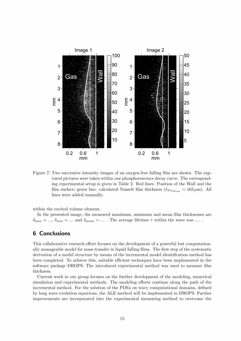
Image 1

mm

mm

0.2 0.6 1

1

2

3

4

5

6

7

810

20

30

40

50

60

70

80

90

100Image 2

mm

mm

0.2 0.6 1

1

2

3

4

5

6

7

85

10

15

20

25

30

35

40

45

50

Gas Wal

l

Gas Wal

lFigure 7: Two successive intensity images of an oxygen-free falling film are shown. The cap-

tured pictures were taken within one phosphorescence decay curve. The correspond-ing experimental setup is given in Table 2. Red lines: Position of the Wall and thefilm surface; green line: calculated Nusselt film thickness (δNuMean

= 163µm). Alllines were added manually.

within the excited volume element.In the presented image, the measured maximum, minimum and mean film thicknesses are

δmax = ..., δmin = ... and δmean = ... . The average lifetime τ within the wave was .... .

6 Conclusions

This collaborative research effort focuses on the development of a powerful but computation-ally manageable model for mass transfer in liquid falling films. The first step of the systematicderivation of a model structure by means of the incremental model identification method hasbeen completed. To achieve this, suitable efficient techniques have been implemented in thesoftware package DROPS. The introduced experimental method was used to measure filmthickness.

Current work in our group focuses on the further development of the modeling, numericalsimulation and experimental methods. The modeling efforts continue along the path of theincremental method. For the solution of the PDEs on wavy computational domains, definedby long wave evolution equations, the ALE method will be implemented in DROPS. Furtherimprovements are incorporated into the experimental measuring method to overcome the

15

limitations due to the low phosphorescence intensity.

Symbol Description

Deff Effective diffusion coefficientDmol Molecular diffusion coefficientDw Diffusion due to wavesFw Wavy source termc concentrationcm Measured concentrationu velocity profileJ generalized molecular fluxJD molecular flux due to diffusionfw model for Dw

θ parametersK1,K2 OperatorsL2 Lebesgue space of square-integrable functionsΩf Time-dependent computational domain

Ω Fixed reference computational domainδ film heightx coordinate in direction of film flowy coordinate in direction of film heightz coordinate in direction of film widtht time

Vl liquid volume flow

References

[1] Adomeit, P. Experimentelle Untersuchung der Stromung laminar-welliger Rieselfilme.PhD thesis, RWTH Aachen, 1996.

[2] Adomeit, P., and Renz, U. Hydrodynamics of three-dimensional waves in laminarfalling films. Int. J. Multiphase Flow 26 (2000), 1183–1208.

[3] Bansch, E. Stabilized space-time finite element formulations for free-surface flows.Numer. Math. 88 (2001), 203–235.

[4] Brauer, H. Stoffaustausch beim Rieselfilm. Chemie-Ing. - Techn 30, 2 (1958), 75–84.

[5] Brooks, A., and Hughes, T. Streamline upwind/Petrov-Galerkin formulations forconvection dominated flows with particular emphasis on the incompressible Navier-Stokesequations. Comput. Methods Appl. Mech. Engrg. 32 (1982).

[6] Donea, J., and Huerta, A. Finite Element Methods for Flow Problems. John Wiley& Sons, 2003.

[7] DROPS package. http://www.igpm.rwth-aachen.de/DROPS/.

[8] Engl, H. W., Hanke, M., and Neubauer, A. Regularization of Inverse Problems.Kluwer Academic Publishers, Dordrecht, 1996.

16

[9] Frenkel, A. L., and Indireshkumar, K. Wavy film flows down an inclined plane:Perturbation theory and general evolution equation for the film thickness. Phys. Rev. E60, 4 (Oct 1999), 4143–4157.

[10] Groß, S., and Reusken, A. Numerical Methods for Two-phase Incompressible Flows,vol. 40 of Springer Series in Computational Mathematics. Springer, 2011.

[11] Hanke, M. Conjugate Gradient Type Methods for Ill-Posed Problems. Longman Scien-tific & Technical, 1995.

[12] Hu, H., and Koochesfahani, M. A novel technique for quantitative temperaturemapping in liquid by measuring the lifetime of laser induced phosphorescence. Journalof Visualization 6, 2 (Jan. 2003), 143–153.

[13] Karalashvili, M. Incremental Identification of Transport Phenomena In LaminarWavy Film Flows. PhD thesis, RWTH Aachen University, 2011. to appear.

[14] Karalashvili, M., Groß, S., Mhamdi, A., Marquardt, W., and Reusken, A.Identification of transport coefficient models in convection-diffusion equations. SIAM J.Sci. Comput. 33, 1 (2011), 303–327.

[15] Karalashvili, M., Groß, S., Mhamdi, A., Reusken, A., and Marquardt, W.Incremental identification of transport coefficients in convection-diffusion systems. SIAMJ. Sci. Comput. 30, 6 (2008), 3249–3269.

[16] Karalashvili, M., Mhamdi, A., Dietze, G. F., Bucker, H. M., Vehreschild,A., Kneer, R., Bischof, C. H., and Marquardt, W. Sensitivity analysis andidentification of an effective heat transport model in wavy liquid films. In Progress inComputational Heat and Mass Transfers, Guangzhou, China (2009), pp. 644–651.

[17] Loffler, K., Gambaryan-Roisman, T., and Stephan, P. Wave patterns in thinfilms flowing down inclined smooth and structured planes. In Proceedings of th 6thInternational Conference on Multiphase Flow (July 2007).

[18] M., B. Stabilized space-time finite element formulations for free-surface flows. Commu-nications in Numerical Methods in Engineering 11 (2001), 813–819.

[19] Marquardt, W. Towards a process modeling methodology, vol. 293 of R. Berber: Meth-ods of Model-Based Control, NATO-ASI Ser. E, Applied Sciences, Kluwer AcademicPub., Dordrecht. Kluwer Academic Pub, 1995, pp. 3–41.

[20] Marquardt, W. Model-based experimental analysis of kinetic phenomena in multi-phase reactive systems. Chem. Eng. Res. Des. 83, A6 (2005), 561–573.

[21] Mudunuri, R. R., and Balakotaiah, V. Solitary waves on thin falling films in thevery low forcing frequency limit. AIChE Journal 52, 12 (2006), 3995–4003.

[22] Panga, M. K. R., Mudunuri, R. R., and Balakotaiah, V. Long-wavelengthequation for vertically falling films. Phys Rev E Stat Nonlin Soft Matter Phys 71 (2005),36310–36311.

17

[23] Ruyer-Quil, C., and Manneville, P. Improved modeling of flows down inclinedplanes. Eur. Phys. J. B 15 (2000), 357–369.

[24] Saad, Y., and Schultz, M. H. GMRES: A generalized minimal residual algorithm forsolving nonsymmetric linear systems. SIAM J. Sci. Statist. Comput. 7 (1986), 856–869.

[25] Schagen, A., and Modigell, M. Luminescence technique for the measurement oflocal concentration distribution in thin liquid films. Experiments in Fluids 38, 2 (Feb.2005), 174–184.

[26] Schagen, A., and Modigell, M. Local film thickness and temperature distributionmeasurement in wavy liquid films with a laser-induced luminescence technique. Experi-ments in Fluids 43, 2 (Aug. 2007), 209–221.

[27] Trevelyan, P., and Kalliadasis, S. Wave dynamics on a thin-liquid film falling downa heated wall. Journal of Engineering Mathematics 50 (2004), 177–208. 10.1007/s10665-004-1016-x.

18