Experimental Investigation of

Added Mass and Damping on a

Model Kaplan Turbine for

Rotor Dynamic Analysis

Timmy Nyman

Civilingenjör, Hållbar energiteknik

2018

Luleå tekniska universitet

Institutionen för teknikvetenskap och matematik

Preface

This report is the main result of my degree project (master thesis) for the Civilingenjör-

sexamen under the program Sustaiable Energy Systems at Luleå Technical University,

LTU. This work is conducted in collaboration with Vattenfall Research and Development

at Älvkarleby, Sweden.

Experiments were conducted in Älvkarleby during the spring and summer of 2017 with

Dr. Berhanu Mulu as head supervisor. Berhanu has introduced me to the project and

helped me patiently during my time in the lab, many thanks! I would also like to thank

Dr. Rolf Gustafsson (VRD), Dr. Erik Lillberg (VRD), Ulf Aurosell (VRD) and Prof. Michel

Cervantes (LTU) for supervision and discussions during the project.

Skellefteå, January 2018

Timmy Nyman

I

Abstract

The concept of added hydrodynamic properties such as added mass is of impor-

tance in modern hydropower development, mainly for rotor dynamic calculations.

Added mass could result in reduced natural frequencies and altered mode com-

pared to existing simulation models. It is of importance to quantify added mass

but also added damping to make the simulation models more accurate.

Experiments are conducted on a model Kaplan turbine, D = 0,5 m, and a steel cube,

S = 0,2 m, for linear vibrations in still water confined in a cylindrical tank. The

experiments are conducted in air and water for evaluation of added forces. The

vibrations are generated with an electrodynamic vibration exciter with a frequency

range of approximately 1-10 Hz with amplitudes 0,5-3 mm.

The experiments were repeated to check test rig reliability. Each individual working

point [frequency, amplitude] were in total tested 40 times in 15 s intervals. The

added mass was found to be function of acceleration for the model Kaplan with

an increase in added mass from 10 % at 4 m/s2 to 35 % at 0,5 m/s2. The damping

forces was at best measured at ±30 %, making added damping calculations unreli-

able.

The cube experiments resulted in small differences between water and air. Cube

results must be interpreted with caution due to test rig uncertainties.

II

Sammanfattning

För att beskriva hur vattnet påverkar turbinen i ett vattenkraftverk kan konceptet

adderade hydrodynamiska parametrar användas. Det är av intresse inom vat-

tenkraftsforskning och viktigt för rotordynamiska simuleringar av rotorsystemet i

ett vattenkraftverk. Adderad massa, dämpning och styvhet kan förändra naturliga

frekvenser och ändra svängningsmoder jämfört med nuvarande simuleringsmod-

eller. Det är viktigt att kvantifiera vattnets påverkan på turbinen genom exempelvis

adderad massa för att förbättra de nuvarande simuleringsmodellerna.

Experiment har genomförts på en model av en Kaplanturbin, D = 0,5 m and en

stålkub, S = 0,2 m, för horisontella vibrationer i stillastående vatten i en cylindrisk

tank. Experimenten har genomförts i vatten och luft för att möjliggöra en utvärder-

ing av de adderade parametrarna. För att vibrera Kaplanturbinen och stålkuben

har en electrodynamic vibration exciter använts med ett frekvensintervall på ca

1-10 Hz med amplituder på 0,5-3 mm.

Experimenten repeterades för att kontrollera testriggens pålitlighet. Varje enskild

arbetspunkt [frekvens, amplitud] testades totalt 40 gånger i intervall om 15 s. Den

adderade massan för Kaplanmodellen fanns vara funktion av acceleration med

en ökning i adderad massa från 10 % vid 4 m/s2 till 35 % vid 0,5 m/s2. Dämpn-

ingskrafterna mättes som bäst till ±30 %, vilket gör beräkningar av adderad dämp-

ning opålitliga.

Experimenten med stålkuben resulterade i en mycket liten skillnad mellan vat-

ten och lufttester. Det här får till följd att resultaten blir svårtolkade på grund av

mätosäkerheter.

III

CONTENTS

1 Introduction 1

1.1 Background . . . . . . . . . . . . . . . . . . . . . . . . . . . . . . . . . . . . . 1

1.1.1 Vattenfall . . . . . . . . . . . . . . . . . . . . . . . . . . . . . . . . . . . 2

1.2 Kaplan Turbine . . . . . . . . . . . . . . . . . . . . . . . . . . . . . . . . . . . 2

1.3 Purpose and Goals . . . . . . . . . . . . . . . . . . . . . . . . . . . . . . . . . 3

1.4 Experimental Limitations . . . . . . . . . . . . . . . . . . . . . . . . . . . . . 4

1.5 Previous Research . . . . . . . . . . . . . . . . . . . . . . . . . . . . . . . . . . 4

2 Theory 7

2.1 Added Mass . . . . . . . . . . . . . . . . . . . . . . . . . . . . . . . . . . . . . 7

2.2 Vibrations and Rotor Dynamics . . . . . . . . . . . . . . . . . . . . . . . . . . 10

2.3 Fluid Structure Interactions . . . . . . . . . . . . . . . . . . . . . . . . . . . . 12

2.4 Numerical Derivation . . . . . . . . . . . . . . . . . . . . . . . . . . . . . . . 15

2.5 Uncertainty Estimation . . . . . . . . . . . . . . . . . . . . . . . . . . . . . . 16

3 Method 17

3.1 Expermimental Setup - Test Rig . . . . . . . . . . . . . . . . . . . . . . . . . . 17

3.1.1 Generating Mechanical Oscillations . . . . . . . . . . . . . . . . . . . 18

3.2 Kaplan Specifications . . . . . . . . . . . . . . . . . . . . . . . . . . . . . . . . 20

3.3 Cube Specifications . . . . . . . . . . . . . . . . . . . . . . . . . . . . . . . . . 21

3.4 Test Design . . . . . . . . . . . . . . . . . . . . . . . . . . . . . . . . . . . . . . 22

3.4.1 Test Design - Kaplan . . . . . . . . . . . . . . . . . . . . . . . . . . . . 23

3.4.2 Test Design - Cube . . . . . . . . . . . . . . . . . . . . . . . . . . . . . 24

3.5 Data Collection and Automation . . . . . . . . . . . . . . . . . . . . . . . . . 25

3.5.1 Force Measurement . . . . . . . . . . . . . . . . . . . . . . . . . . . . 25

3.5.2 Displacement Measurement . . . . . . . . . . . . . . . . . . . . . . . 26

3.6 Post Experimental Analysis in Matlab . . . . . . . . . . . . . . . . . . . . . . 27

3.6.1 Approximation or Smoothing . . . . . . . . . . . . . . . . . . . . . . . 29

3.7 Experimental and Analysis Algorithm . . . . . . . . . . . . . . . . . . . . . . 30

4 Results 32

4.1 Test Rig Functionality . . . . . . . . . . . . . . . . . . . . . . . . . . . . . . . 32

4.1.1 Frequency Deviations . . . . . . . . . . . . . . . . . . . . . . . . . . . 32

4.1.2 Test Rig Resonance . . . . . . . . . . . . . . . . . . . . . . . . . . . . . 33

4.1.3 Amplitude Uncertainty . . . . . . . . . . . . . . . . . . . . . . . . . . 35

IV

4.2 Experimental Results - Kaplan . . . . . . . . . . . . . . . . . . . . . . . . . . 36

4.2.1 Added mass - Kaplan . . . . . . . . . . . . . . . . . . . . . . . . . . . . 37

4.2.2 Added Damping - Kaplan . . . . . . . . . . . . . . . . . . . . . . . . . 39

4.3 Experimental Results - Cube . . . . . . . . . . . . . . . . . . . . . . . . . . . 40

4.3.1 Simulations Compared to Cube Measurements . . . . . . . . . . . . 42

5 Discussion 44

5.1 Repeatability and Uncertainties . . . . . . . . . . . . . . . . . . . . . . . . . 44

5.2 The Shaker . . . . . . . . . . . . . . . . . . . . . . . . . . . . . . . . . . . . . . 44

5.3 Hydrodynamic forces . . . . . . . . . . . . . . . . . . . . . . . . . . . . . . . . 44

5.3.1 Added Mass . . . . . . . . . . . . . . . . . . . . . . . . . . . . . . . . . 45

5.3.2 Added Damping . . . . . . . . . . . . . . . . . . . . . . . . . . . . . . . 45

5.4 Rotor Dynamics and Simulation Models . . . . . . . . . . . . . . . . . . . . 45

6 Conclusion 46

V

NOMENCLATURE

Symbol Description Unit

m Mass kg

ma Added mass kg ,%

Mi j Added mass matrix −ρ Density kg /m3

U Velocity m/s

g Acceleration due to gravity m/s2

T Torque N m

L Length m

R Radius m

A Amplitude of vibration m

AD Area m2

A j Acceleration vector m/s2, r ad/s2

J Rotational inertia kg m2

F Force N

Fw ater Force signal (data) for water tests N

Fai r Force signal (data) for air tests N

Fa,max Force at maximum acceleration N

Fv,max Force at maximum velocity N

x, y Displacement (length) m

x, y Velocity m/s

x, y Accleration m/s2

t Time s

ta,max Time at maximum acceleration s

tv,max Time at maximum velocity s

a Acceleration m/s2

α,γ Angular acceleration r ad/s2

k Stiffness N /m

ka Added stiffness N /m,%

K Stiffness matrix N /m

c Damping N s/m

ca Added damping N s/m,%

C Damping matrix N s/m

VI

Symbol Description Unit

ω Angular frequency r ad/s

ωn Natural frequency r ad/s

f Frequency of vibration 1/s

Re Reynolds Number −Re f Reynolds Number for vibrations −CD Drag coefficient −

Working point - Specific vibration amplitude and frequency

Shaker - Abbreviation for the Electrodynamic exciter used in the experiments

VRD - Vattenfall Research and Development

VII

1 INTRODUCTION

This section introduces necessary background to hydropower, turbines, Vattenfall and

added mass. The goals and limitations for the project are also outlined.

1.1 Background

In Sweden, hydropower has been a major contributor to the energy mix since the first

notable plants were established at the beginning of the 20th century. During the last

decade the hydropower gross production has been 30-50 % of the total electricity supply

in Sweden [1]. The variations in production is manly due to water availability.

Hydropower plants was originally designed and built to supply a steady base of elec-

tricity during quasi-steady operating conditions (i.e quasi-steady discharge flow) [2].

Over the years hydropower operation has shifted towards peak regulation of the grid

because of the large storage capacities associated with the dams. In the past decade

the increasing amount of installed wind power and the predicted instalments due to

national green-energy targets will further put pressure on the hydropower plants.

The new operating conditions means that load variation, start-stop and load rejection

will increase. The increasing transient and off design operation conditions can cause

numerous problems such as blade and bearing damage [3]. Damage can be caused by

turbine to discharge ring collisions which introduces unwanted external forces [4].

Reduction in hydraulic efficiency at off design operation conditions must also be consid-

ered to reduce losses (energy and economical). The new more unpredictable operating

conditions and the in general aging machine park (in Sweden) are motivating factors

for hydropower research in the beginning of the 21th century [2].

The dynamic analysis of the rotor system has become even more important because of

the above topics. Good modelling of the rotors can prevent failure and more accurately

predict rotor life time. In the rotor models consideration must be taken to the runner-

water interaction. The phenomena mainly discussed is the concept of added mass, it

is mentioned in M.Nässelquists PhD where it is listed as a topic for further research

[5]. The added mass can be seen as a mass added to the runner due to acceleration of

the fluid around it. This added or apparent extra mass affects the dynamic analysis by

reducing natural frequencies and altering mode shapes. The effect of added mass is

1 of 48

not well studied in hydropower and it is common that designers use a standard value

of added mass as rule of thumb. The constant value of 25% added mass has been

mentioned as a reasonable assumption [5]. The added damping is rarely mentioned at

all and is neglected in simulations. Due to the limited knowledge about hydrodynamic

forces in hydro turbines it is an interesting research topic and consequently the topic of

this thesis.

1.1.1 Vattenfall

Vattenfall Vattenkraft AB is the largest operator on the Swedish hydropower market with

around half of the total national installed capacity. The large holdings are an incentive to

extensive researches too ensure a high operation efficiency, return and safety. Research

is conducted by Vattenfall Research and Development and experiments are conducted

at the laboratory in Älvkarleby. The research focus concerning the hydropower portfolio

are partly on dam models, turbine model testing, rotor dynamics and fish migration

issues.

1.2 Kaplan Turbine

The Kaplan turbine will now briefly be introduced (for information about Francis and

Pelton turbines, see [6]). It was invented around 100 years ago by Viktor Kaplan as

a development of and a complement to the already existing Francis turbine. Kaplan

turbines are designated as reaction turbines. The pressure due to the upstream water

head is converted across the turbine and transferred to the rotor as mechanical power

in the form of torque and angular velocity. Figure 1 shows one variant of the Kaplan

turbine. Differences can be found in the number of blades, the blade design and the

shape of the runner crown. The most important feature associated with Kaplan turbines

is the ability to adjust blade angles accordingly to the incoming water flow. This results

in a higher efficient over a larger range of discharge rates compared to fixed blade

Francis turbines. The Kaplan turbine is adapted for low head i.e high specific speeds

[6]. The wide operating range at low heads makes it a good choice for many Swedish

hydropower stations.

2 of 48

Figure 1: The model Kaplan used in the experiment. The larger version of the model (theprototype runner) is installed in Porjus, Luleälven.

The relation between the guide vane position (i.e discharge rate) and the blade angles

are commonly refereed to as the combination of the turbine. The combination can be

determined experimentally, via an index test, and implemented in the turbine control

system. This is a crucial part to ensure a good machine efficiency [7]. Regarding the

dynamic modelling of the rotor the operating conditions may influence the system re-

sponse due to a correlation between added parameters and rotational speed, suggesting

blade angle could influence added parameters [8].

1.3 Purpose and Goals

The work in this thesis is focused on an experimental approach for determining how

the parameters (e.g vibration frequencies and amplitude) and conditions (e.g. object

geometry) affect the added mass and damping. An increased knowledge regarding

the added mass term from the turbine-water interaction could improve rotor dynamic

modelling. In the future such improvements could improve the rotor lifetime. One aim

is to determine how well the test rig is running from a repeatability point of view.

The goal is to generate a dataset with statistical significance and to present the results in

a compact form suitable for a sequent rotor dynamic analysis. The idea is to determine

3 of 48

the added parameters experimentally for later verification of numerical models. The

result is a quantification of the added mass and added damping terms in the mass and

damping matrices used in the rotor dynamic analysis (with reservations for experimen-

tal limitations).

1.4 Experimental Limitations

In general, most types of measurements on full scale hydropower are difficult due to a

number of factors. The main difficulties are associated with availability and cost issues.

Therefore model testing is widely used in hydropower and turbine research, due to

increased availability and reduced costs. At Vattenfall R&D’s laboratory in Älvkarleby a

test rig has previously been constructed called the "Added Mass Test Rig". The test rig

enables model testing using rectilinear vibrations in still water. The added mass test rig

will be used for the experiments in this project and thereby significantly restricting the

research by reducing the degrees of freedom and simplifying the boundary conditions.

A measurement system has also been designed in labVIEW by VRD staff. At the project

start it was decided that VRD staff should be consulted for problems, questions or

improvements concerning the measurements system.

1.5 Previous Research

The concept of added mass has been studied in fluid mechanics over the years e.g. by

Maxey and Riley in 1982 who investigated the equation of motion for a sphere in non-

uniform flow [9]. In naval and ship engineering the added mass has been investigated

since the mid 20th century. In 1970 Salvesen et al. presented updated theory and a

computer program for calculation of ship motions and loads [10]. The concept of the

6-DOF mass and damping matrix was included. The added mass concept was reviewed

in 1983 by Brennen who discussed the added mass matrix and theory limitations. He

mentioned the influence of compressibility, viscosity, the distance to solid boundaries

and free surfaces as factors influencing added mass. [11].

Added mass is a phenomena found in the area of research called Fluid Structure In-

teraction, FSI. The theory presented is usually not applicable for analytical solutions

of engineering problems. Numerical simulations are therefore the preferred working

method. In a review by Chirag [3] five numerical and experimental studies on turbine-

fluid interaction were compared. The experiments were conducted in still water and

4 of 48

air and were focused on modal analysis by investigating mode shapes and reduction in

natural frequencies. The reduction in natural frequency from air-water was 12-64 %.

The numerical results differed 1,5-15 % from the experimental results.

Rodriguez et al. [12] submerged a Francis turbine in still water and used accelerometers

to find the natural frequencies and mode shapes. The runner was excited in air and

water with an impact hammer. The natural frequencies was reduced by 11-38 % and

the added mass was calculated to 27-264 % for the different mode shapes. The first

detected natural frequency, in water, was at 279,5 H z. The relevance of these results are

questionable since the vibration frequencies of a prototype runner are excepted to be

lower.

The importance of added mass but also added damping and stiffness arises in the field

of rotor dynamics, where analysis of hydropower rotors are of great interest. In Näs-

selqvist’s PhD thesis it was stated [5] that the added properties are of importance in the

modelling of the system response. The added properties are included as vague estimates

or completely disregarded in the existing models. The research on hydropower rotor

dynamics is relatively new and the research has mainly been focused on bearings and

rotor-stator interactions.

During 2016 a degree project was conducted on the test rig at Älvkarleby laboratory. The

thesis was aimed at simplified theoretical interpretation of FSI and the construction of

the Added Mass Test Rig [13]. The experimental results showed that it was possible to

measure added mass. The damping results were questionable. However, the results was

based on a narrow dataset and the reliability of the test rig was questioned. Another

degree project was conducted in parallel but independently [14]. This thesis focused on

simplified (cylinder and disk) turbine simulations in CFX with two way coupled simula-

tion and acoustic coupled simulation. The acoustic simulations had a maximum 4 %

difference compared to experiments previously conducted. The maximum difference

between the two methods was 14 % for the simulations in water.

Despite the conducted research there are a number of unanswered questing regarding

the added mass concept such as [3]:

• Added mass in a flow situation similar to the working conditions of a turbine

runner.

5 of 48

• Influence of solid boundaries and surfaces.

• A connection between model and prototype in terms of up-scale limitations.

• Added mass below the turbine runner natural frequencies and its impact on the

rotor dynamic analysis. For example added mass as function of acceleration or

Reynolds number.

Most of the previous research has been conducted by considering turbine natural

frequencies and mode shapes. The determination of added mass and damping as a

function of acceleration and velocity respectively, suitable for rotor dynamic analysis

has not been attempted before the pilot project in Älvkarleby 2016.

6 of 48

2 THEORY

Some theory will now be introduced, starting with an introduction of the added mass

concept. An explanation will also be given on how the added parameters are derived

from the experiments.

2.1 Added Mass

The added mass term is used in physics and fluid mechanics to describe the added or

apparent mass for an object which is accelerated in a fluid. The added mass should not

be confused with the more common concept of drag force. The drag force is the force

acting on an object in a fluid at constant relative velocity between the fluid and object

accordingly to,

FD = 1

2ρU 2 ADCD . (1)

In equation (1) the drag coefficient, CD , is a cumulative constant describing the re-

sistance. The coefficient is manly consisting of the two major factors influencing the

drag force which is skin friction and form drag. The drag force is extensively studied

experientially and with CFD. Accurate analytical calculations are hard to perform for

real world applications.

The added mass can be interpreted simply by considering newtons 2nd law of motion,

F = (m +ma) · dU

dt. (2)

For an object accelerating in a fluid the mass, ma , in equation (2) is considered the

added or apparent extra mass of the object, a result of the extra kinetic energy needed

to accelerate the fluid. The real mass of the object obviously remains the same and

does not affect the added mass. The added or apparent mass should be though of as an

imaginary cumulative added mass due to the acceleration of fluid around the object.

In theory the added mass is proportional to the fluid density and the geometry of the

object.

The added mass can in some simple and idealized situations be calculated analytically.

If an ideal potential flow is considered the added mass for a cylinder in linear motion is

7 of 48

described by,

ma = ρπR2L. (3)

In this particular case the added mass is equal to the displaced fluid volume and the

added mass is constant with respect to the acceleration of the object. The added mass is

clearly proportional to density. This implies that the relative difference between added

mass for air and water is in the order 103. For engineering applications the added mass is

generally investigated experimentally to obtain accurate results, where idealized theory

could serve as a guideline.

For a general body with 6 DOF the added mass can be described with an added mass

matrix. When an object is subjected to acceleration in one direction it is not limited to

motion in that direction. Acceleration in the three translational and rotational directions

are possible [11]. The forces, F , and moments, M , corresponding to these accelerations

is called the resultant, Ri , where i = 1,2,3 are linear forces and i = 4,5,6 are moments.

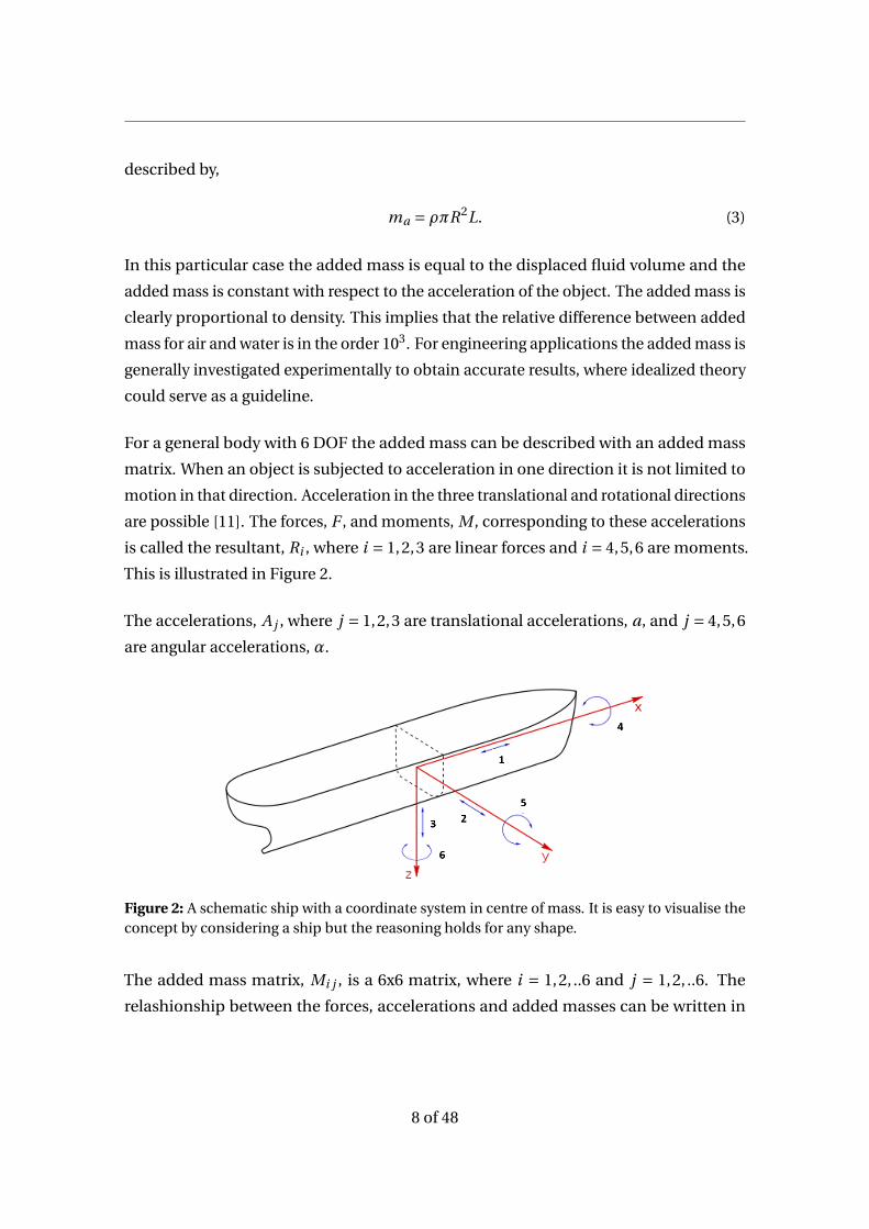
This is illustrated in Figure 2.

The accelerations, A j , where j = 1,2,3 are translational accelerations, a, and j = 4,5,6

are angular accelerations, α.

Figure 2: A schematic ship with a coordinate system in centre of mass. It is easy to visualise theconcept by considering a ship but the reasoning holds for any shape.

The added mass matrix, Mi j , is a 6x6 matrix, where i = 1,2, ..6 and j = 1,2, ..6. The

relashionship between the forces, accelerations and added masses can be written in

8 of 48

tensor form as,

Ri = Mi j A j . (4)

The mass elements in Mi j can be thought of as added mass in direction i due to an

acceleration in direction j . The dimensions of the added mass matrix in equation

(4) must be clarified since equation (4) is not justified for only mass (kg SI-unit) as

dimension in the added mass matrix.

Expanding the tensors yields,

F1

F2

F3

T4

T5

T6

=

kg kg kg kg ·m kg ·m kg ·m

kg kg kg kg ·m kg ·m kg ·m

kg kg kg kg ·m kg ·m kg ·m

kg ·m kg ·m kg ·m kg ·m2 kg ·m2 kg ·m2

kg ·m kg ·m kg ·m kg ·m2 kg ·m2 kg ·m2

kg ·m kg ·m kg ·m kg ·m2 kg ·m2 kg ·m2

·

a1

a2

a3

α4

α5

α6

. (5)

The units of the added mass matrix Mi j are displayed in equation (5). The rotating

inertia is included in 9 position and for clarification it would be called added rotating

inertia.

The added mass matrix can be reduced by geometrical similarity or by locking degrees

of freedom. By locking A j for j = 2−6. The problem reduces to,

F1

F2

F3

T4

T5

T6

=

m11

m21

m31

m41

m51

m61

·[

a1

]. (6)

In the available test rig the motion is strictly linear and the measurements are restricted

to F1. The expression is thereby similar to the original expression in equation (2). When

geometrical similarity is assumed it is clear that m11 = m21. The information in this

section is analogous for the added damping, only with changes of symbols and units.

9 of 48

2.2 Vibrations and Rotor Dynamics

Added mass and damping influences the dynamic analysis of a system. To clarify this a

simple single degree of freedom system can be considered.

The classical general equation of motion for a SDOF system for free vibrations is ex-

pressed as a force equilibrium using newtons laws,

mx + cx +kx = 0 (7)

The stiffness is modelled with, k (N/m), and together with the mass (m) of the object

the undamped natural angular frequency can be determined,

ωn =√

k

m. (8)

The damping, c (Ns/m), is associated with the energy dissipation of the system. The

amount of damping in a system is usually quantified with the damping ratio witch is

defined as,

ζ= c

2p

k ·m. (9)

The system described by equation (7) is a idealized system operating i vacuum. When a

fluid and driving force is introduced to the model the additional added fluid forces will

affect the system response. This can simply be modelled as [2],

mx + cx +kx = F (t )−ma x − ca x −ka x, (10)

The fluid forces are opposing the motion by possibly increasing the rate of energy

dissipation, depending on the ratio between added mass and damping, seen in equation

(9). A reduction in the undamped natural frequency is inevitable, as seen in equation

(8). Rearranging the terms in equation (10) to,

(m +ma)x + (c + ca)x + (k +ka)x = F (t ). (11)

The added mass, ma , is a result of the phenomena described in section 2.1 equation (2).

The added damping, ca , can simply be described as the extra force it takes to push an

10 of 48

object at constant velocity in water compared to air, comparable to equation (1). Added

stiffness is harder to describe for an incompressible fluid in a control volume with open

boundaries. It should not exist at those conditions in the counter axial direction. How-

ever, when considering vibrations in close proximity to a solid boundary or vibrations

in the axial directions, stiffness effects could be present.

The added parameters must be determined to accurately predict the system response.

The principal idea in this thesis is to displace the object in equation (11) at a sinusoidal

manner and determine the difference in required force between air and a denser fluid

such as water. The difference in force will be utilized to determine the added parameters.

The object displacement curves will be the same in both cases.

Equation (11) is a simple SDOF system but can be expanded to a MDOF system if the m,

c and k are expanded to matrices, M, C and K.

Rotor dynamics is usually treated as its own field due to the added dynamic complexities.

In the simplest cases equation (11) can be converted to a rotating system by appropriate

unit substitutions. The torsional vibration analysis is the first logical step towards rotor

dynamics.

When considering rotor dynamic modelling and especially the rotor system in a hy-

dropower plant some of the main difficulties with the modelling is:

• Gyroscopic effects

• Unbalance

• Rotor-stator interaction

• Modelling of bearings

• Fluid forces at the runner e.g. added mass

These phenomena must be included in the equation of motion to accurately model the

system response. A first approximation of a hydropower rotor model could be [5],

M x + (C +ωG)x +K x = F (t )+FG . (12)

The model includes the gyroscopic matrix G, a time dependant force vector F(t), and a

11 of 48

constant force vector F(G). This is usually solved for 4 degrees of freedom x, y, α and γ.

The mass matrix in equation (12) is expanded for the simplest case,

M x =

m · · ·· m · ·· · J ·· · · J

·

x

y

α

γ

(13)

The objective is to find the added properties in the mass matrix as a function of the

acceleration, for implementation in equation (13). The experimental setup can measure

the added mass in the x and y directions only i.e mass elements on the diagonal. The

rotational inertia terms can not be predicted with the current test rig.

2.3 Fluid Structure Interactions

In the field of Fluid Structure Interactions the boundary between solid and fluid are

of interest. The forces and the interaction between solid to fluid and vice versa are

the primary focus. In numerical simulations this coupling between solid and fluid is

modelled and an appropriate mesh is constructed adapted to the method in question.

In the analysis of the governing equations a connection must be found between the

solid and fluid forces. In the previous thesis written on the added mass test rig a major

part of the objective was to derive simplified equations describing the hydrodynamic

forces i.e the added parameters. The equations, simplifications and assumptions used

in the derivation are summarized below:

• Fluid Domain

– Continuity equation.

– Navier-Stokes equation.

– Stress tensor for a Newtonian fluid.

• Solid Domain

– Oscillatory motion with mass, damping and stiffness.

• Simplifications and Assumptions

12 of 48

– Newtonian fluid.

– Incompressible fluid.

– Flow in one direction U(u,v,w)=U(u,0,0).

– Introducing a number of non-dimensional parameters.

– Perturbation expansion for trend visualization.

The result of the derivation is an analytical expression for determining the hydrody-

namic forces by using the above equation and assumptions [13]. The expression could

be used to estimate the behaviour of the solid to fluid interaction for simple geometry’s.

It is not seen as practically possible to evaluate the equations for a Kaplan runner, at

least within a reasonable time frame. And it is not the in the scope of this thesis.

However a number of conclusions useful in the experimental process can be stated. In

the process of non-dimensioning the Naiver-Stokes equation a version of the Reynolds

number was found to be,

Re f =ρωA2

µ. (14)

Where , ω, is the angular frequency of vibration and, A, the vibration amplitude. In

general the Reynolds number is interpreted as,

Re = Inertia forces

Viscous forces(15)

Inertia forces are related to some mass and acceleration and viscous force to some

viscosity and velocity. It was concluded by Jakobs derivations that the relative size of the

hydrodynamic forces follows the conventional interpretation of Reynolds number. The

following conclusions can be draw as benchmarks before conducting experiments:

• At low Re f the viscous forces i.e damping forces dominates.

• At high Re f the inertia i.e mass forces dominates.

• Increasing the amplitude and frequency increases the hydrodynamic forces.

• These is a cross-over zone were the interia and viscous forces are similar in size.

• In general, inertia forces dominates in relative size.

13 of 48

• When oscillatory motion is driving an object submerged in a fluid the pure inertia

force (related to added mass) is found at maximum acceleration and the pure

viscous force is found at maximum velocity, see Figure 3.

Figure 3: A typical object displacement signal when oscillated. The points of maximum acceler-ation and velocity are highlighted.

The maximum force components are found in the measured force signal at F (tamax ) and

F (tvmax ). The hydrodynamic forces are simply calculated by,

Fa,max = Fw ater (tamax )−Fai r (tamax ) (16)

and

Fv,max = Fw ater (tvmax )−Fai r (tvmax ). (17)

The added mass and added damping are directly calculated as,

ma = Fa,max

amax(18)

and

ca = Fv,max

vmax(19)

14 of 48

The next step is to determine how the inertia forces and viscous forces should be

distributed between the maxima. The distribution of force components during one

period of translation is important for the sequent rotor dynamic analysis. It is of interest

to see how the added properties are distributed during one period for a specific Re f

or acceleration. The force components are assumed to have an elliptical distribution

during a period of motion. The force component contributing to added mass is,

Fa = Fa,max · si n(w t ). (20)

The component contributing to added damping is,

Fv = Fv,max · cos(w t ). (21)

The total added force could be estimated accordingly to,

F 2tot = F 2

v +F 2a . (22)

2.4 Numerical Derivation

In the experiments the motion of the model turbine is driven by sinusoidal oscillations.

The translational position in direction x can be described by,

x = Asi n(ω · t ) (23)

Taking the time derivative of x yields the velocity,

x = Aωcos(ω · t ), (24)

and the time derivative of velocity is acceleration,

x =−Aω2si n(ω · t ). (25)

The theoretical continuous analysis is simple but must be performed on discrete exper-

imental data as well. By using numerical derivation the derivatives can be expressed

15 of 48

as,

S(x +h)−S(x −h)

2h= S′(x)+O(h2). (26)

In the central difference approximation in equation (26), S, represents the discrete signal

and h represents the time step associated with the sample rate. For the endpoints the

backward and forward approximations are utilized. When using numerical derivatives

consideration must be taking to the truncation and number representation errors which

will occur, usually as function of the sample rate h.

2.5 Uncertainty Estimation

The uncertainty of the sensors and/or measurement chains must be calculated. The

aim is to assign a value to each sensor which quantifies the uncertainty. The uncertainty

is expressed as RSS,

Uc =√

n∑i=1

u2i . (27)

Where n is the total number of sub uncertainties. The uncertainty, ui , could be either

relative or absolute. Equation (27) is used to combine uncertainties like hysteresis,

resolution and temperature effects for the sensors.

When the uncertainty in measured data from repeated experiments is evaluated the

standard deviation,

σ=√√√√ N∑

i=1

1

N(yi −Y )2, (28)

is used. Where N is the number of data points and Y the average accordingly to,

Y = 1

N

N∑i=1

yi . (29)

By using Equation (28) the uncertainty on the measurand is quantified with respect to

the whole test rig.

16 of 48

3 METHOD

The overall experimental approach is to measure forces on an object in air and water

separately. When the forces are compared the influence of friction and inertia will

cancel out. The result after comparing water and air test are a quantification of the

hydrodynamic forces acting on the object in motion.

The experiments are now described together with a description of the test design. The

data collection and analysis is described for the determination of hydrodynamic forces

and added mass.

3.1 Expermimental Setup - Test Rig

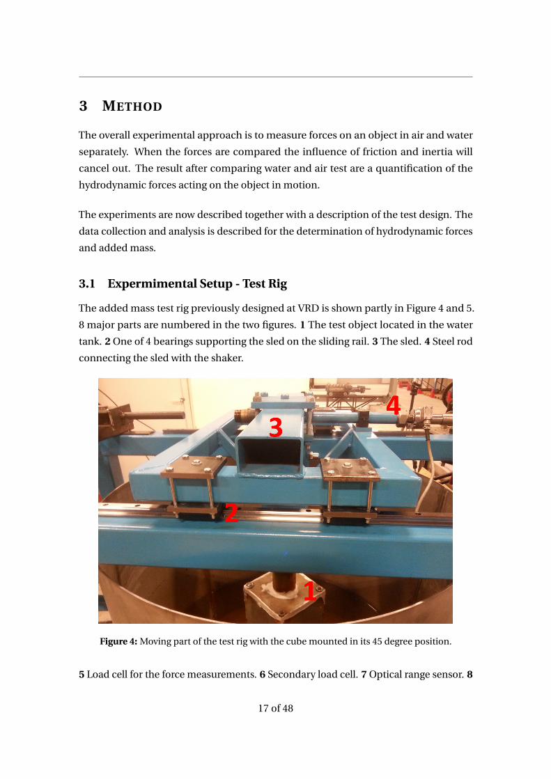
The added mass test rig previously designed at VRD is shown partly in Figure 4 and 5.

8 major parts are numbered in the two figures. 1 The test object located in the water

tank. 2 One of 4 bearings supporting the sled on the sliding rail. 3 The sled. 4 Steel rod

connecting the sled with the shaker.

Figure 4: Moving part of the test rig with the cube mounted in its 45 degree position.

5 Load cell for the force measurements. 6 Secondary load cell. 7 Optical range sensor. 8

17 of 48

Shaker.

Figure 5: The shaker, measurements devices and the rod the connecting shaker and sled.

The sled and shaker are supported by a rigid steel frame which is bolted to the concert

floor at 8 places.

The test rig is positioned in one of the halls at VRD in Älvkarleby where a few other

experiments are running. No external experiment, component or parameter in the hall

is assumed to influence the experiment on a measurable level. The only parameter with

theoretical potential to influence the measurements is the indoor temperature which

can not be controlled by the author. It is estimate to vary between 18-23 °C for any given

day. The air temperature has the potential to change the density and kinematic viscosity

of the water in the tank and offset measurement devices.

3.1.1 Generating Mechanical Oscillations

The test object and sled configuration must be excited in some controlled manner.

Oscillation at a sinusoidal path is a natural way of doing this. As seen in Figure 5 an

electrodynamic vibration exciter (shaker) ,Type SW 1507, is mounted on the test rig. It

was mentioned in the previous thesis that the shaker might not be the best choice for

this particular experiment. The shaker is mainly intended for smaller loads at higher

frequency and some problems may occur at higher loads and lower frequencies.

18 of 48

In the previous thesis it was proposed that another exciter source could be used to

improve the test rig. Therefore, an attempt was made to implement a hydraulic cylinder

as the oscillation source, in the beginning of the project. It was mounted on the opposite

side of the sled, seen from the shaker and connected to the sled. The hydraulic cylinder

was connected to a complete control system with a hydraulic pump, oil tank, computer

control etc. In the attempt to regulate the sleds motion in a sinusoidal manner it was

realised that the hydraulic cylinder/control system could not control the output good

enough. The small displacement amplitudes and relative high frequencies were to

challenging for the hydraulic pump and cylinder configuration. Basically, the control

information is transmitted with oil which introduces problems with viscosity and valve

closure times.

It was finally decided to abandon the hydraulic cylinder and instead make use of and

evaluate the all ready installed shaker, with the notion that some problems may exist.

19 of 48

3.2 Kaplan Specifications

The experimental setup for the Kaplan runner (without sled) is shown in Figure 6.

Figure 6: Schematic setup of the runner submerged in the water tank.

The model Kaplan runner has previously been used by VRD in the turbine testing

laboratory. The main runner parameters are listed in Table 1.

Table 1: Main parameters for the model Kaplan runner.

Parameters Symbol Size and Unit

Runner diameter D 500 mm

Runner height H 396 mm

Runner weight mr 50 kg

Number of blades Z 6

Material - Brass

Blade angle α 1.7◦

20 of 48

3.3 Cube Specifications

The Cube is mounted in a similar way as the Kaplan model. The specifications are listed

in Table 2.

Table 2: Main parameters for the cube.

Parameters Symbol Size and Unit

Side of cube S 20 cm

Cube weight (hollow) mr 8 kg

Installation angle φ 0, 45◦

Material - Stainless steel

The installation angle, φ = 0, means that a side of the cube is perpendicular to the

direction of motion as can be seen in Figure 7.

Figure 7: Top view of cube positions relative to the direction of motion.

21 of 48

3.4 Test Design

There are a number of variables potentially influencing the experiment. If consideration

is taken to the experimental setup the variables in Table 3 are an attempt to order

variables by influence and relevance in the experiment. The order of the list should

be seen a list of priorities based on assumptions from previous research. During the

experiments some of the variables have been varied to determine their impact. Other

variables have been keep constant due to time and /or test rig limitations.

Table 3: Parameters thought to influence added variables listed by probable relevance.

Variables Symbol Unit Handling of variable in experiments

Geometry of the object - - Varied

Displacement A mm Varied

Frequency f Hz Varied

Clearance c mm Constant

Distance to free surface h1 mm Constant

Distance to bottom of tank h2 mm Constant

Water temperature Tw °C Constant

The two distances h1 and h2 (the distance to surface and bottom of the tank) are

interesting in the sense that the could influence this specific experiment for lateral

vibration. In an experiment simulating a more realistic situation these parameters lack

meaning since they do not exist. However, in a real situation the water head is of large

interest, but Figure 6 is not a good representation of turbine water head.

The experiment was designed by also taking the following topics and constrains into

consideration:

• Working range of shaker

– The shaker has a frequency range of roughly 0,5-10 Hz and a displacement

amplitude of 0,25-2,5 mm, depending on the system configuration.

• Time management

– There are concerns that the shaker might be overheated during operation so

continuous tests are limited to 1-2h, to reduce the risk of overheating.

22 of 48

• Check for repeatability

– The experiment must be repeated several times to check the repeatabil-

ity of the experimental setup and to enable a good quantification of the

measurand.

• Constraints of existing measurement system

– The amplitude input to measured output will vary slightly over time. Due to

regulation error and shaker instability.

• Enable check of reproducibility

– Previous measurements and simulations have been performed and compar-

ing results are desirable.

3.4.1 Test Design - Kaplan

The experimental test sequence for the model Kaplan runner consists of 7 frequencies

with 10 amplitudes for each frequency, resulting in 70 working points. The frequencies

and amplitudes that were used as inputs to the system are listed in Table 4. The shaker

starts at 0,5 Hz and ramps the amplitude from 0.2-2.9 V in 15 s intervals. The rest of the

operation follows the same logical order. The voltage is experimentally derived to at

best cover the operation range of the shaker at each frequency.

Table 4: The shaker inputs used in the experiments for the model Kaplan.

f (Hz) A (V)

0.5 0.2-2.9

1 0.2-2.9

2 0.2-2.9

3 0.2-2.3

4 0.3-1.7

5 0.3-1.1

6 0.2-0.9

In one test the operation scheme in Table 4 is run 4 consecutive times. After a test the

rig is stopped and data saved. In total 10 of these tests are performed for air and water

respectively. The 70 working points are thereby repeated 40 times for air and water

23 of 48

respectively. Total effective run time for the water and air tests combined are around 20

h plus an additional 2-3 for water refill/drain.

For each working point data is collected during a 15s interval. During the amplitude

ramp-up for a certain frequency the system stabilises quickly and data is logged continu-

ously. The first second of data is removed as a precaution, but no long term disturbances

in the outputs has been found when the amplitude is incrementally increased (com-

pared to start-up for completely still water). When the frequency changes and amplitude

drops (accordingly to Table 4) the new frequency is phased in with the water before data

is collected, to avoid disturbances from the remaining energy in the water.

3.4.2 Test Design - Cube

The experiments with the cube was conducted accordingly to the same procedure as for

the Kaplan model but with a wider range of frequencies, seen in Table 5.

Table 5: Settings used in the experiments for the Cube.

f (Hz) A (V)

1 0.2-2.9

2 0.2-2.9

3 0.2-2.3

4 0.3-1.7

5 0.3-1.1

6 0.2-0.9

7 0.2-0.9

8 0.2-0.9

9 0.2-0.9

24 of 48

3.5 Data Collection and Automation

The control and measurements system is built in labVIEW by VRD staff. The new system

is automatized in the sense that it allows for inputs such as the data in Table 4. The data

is automatically saved during operation for each working point in individual .l vm files

to simplify data management. The measurement system is designed to keep the shaker

fixed (oscillation around a set point) in the axial direction and keep the output steady

during the operation for a working point. Previous experiments was conducted by the

tedious task of pressing a run button and manually creating data files for each working

point.

Data is throughout all tests sampled at 250 Hz. When the sample rate is increased above

250 Hz the computers CPU is not fast enough and the input signal to the shaker lags

behind. Considering the shaker frequencies and the chosen analysis method the sample

rate is adequate.

The two measured quantities are force (N) and displacement (mm). The position of the

measurement equipment can be seen in Figure 5.

3.5.1 Force Measurement

The force was measured across the rod which connects sled and shaker. The load cell is

a HBM load cell type U2, with max cap. at 100 kg. The load cell is of strain gauge type

and uses a full Wheatstone bridge, where the output voltage is proportional to the load.

The force signal is amplified before it is converted to digital in the National instruments

high speed cDAQ-9174. Calibration is done with the calibration system and control

weights used in the turbine model testing lab. The load cell is carefully mounted to

awoid misalignment. The load cell uncertainty is given related to full scale and to the

actual measured value. The total relative uncertainty depending on the measured value

is shown in Figure 8.

25 of 48

Figure 8: The relative uncertainty for the load cell as function of the measured load.

In the mounting process, with a screw joint, tensions will inevitably be applied to the

load cell offsetting the measurements. This is handled in Matlab by normalizing the

offset to zero.

A secondary load cell was placed on the rod as means on verifying the primary load cell.

The secondary load cell was not directly used in the measurements. It was used as a way

to verify and check for systematic errors with the primary load cell.

The load cell is calibrated against mass (kg) which means that conversion to force is

necessary. The force is calculated with an acceleration due to gravity of 9,81 m/s2 for all

data.

3.5.2 Displacement Measurement

The displacement was measured directly on the moving element of the shaker by a

optical sensor, optoNCDT 1402-50, which is based on the principle of triangulation.

The measurement range is 50 mm. The sensor is mounted directly on the steel frame.

The steel frame was checked for movement to avoid problems with the displacement

measurement. No difference was found when the sensor was mounted independently

from the steel frame. The sensor was previously calibrated by the authors supervisor.

The uncertainty is ±0.15 % FS, which in this case leave a uncertainty of ±20 µm. The

influence of uncertainty on the measured value can be seen in Figure 9.

26 of 48

Figure 9: The relative uncertainty for the optical displacement sensor as function of the mea-sured displacement.

The uncertainties are related to full scale which means that the measurements are

heavily influenced when the measured value is low, as seen in Figure 9 at 0,2 mm.

3.6 Post Experimental Analysis in Matlab

The analysis in Matlab contains two major parts. 1 Extracting the relevant quantities

from raw data by approximation. 2 Interpret the acquired data, plot and analyse results.

To allow for a structured data analysis the data was approximated/filtered and averaged.

For each working point the data was approximated with Fourier transform i.e the basic

sine from the FFT algorithm. This is a necessity because the derivatives of the raw signal

can become highly noisy. The maximum acceleration and velocity are found in the

displacement signal, accordingly to Section 2.4, and the corresponding forces can be

collected from the force signal, as seen in the example in Figure 10. The phase shift

between the force and displacement signal corresponds to the distribution of inertia

and viscous forces. An increase in viscous forces increase the phase shift.

27 of 48

Figure 10: Example of how the forces are determined when the displacement and force signalare phase shifted due to the distribution of inertia and viscous force.

The magnitude or amplitude of the fft-analysis for the displacement and force signal is

thought of as the average amplitude in force and displacement for that working point

(even is the terminology ’average’ can be discussed in this case). This procedure is

repeated for all working point and all tests. The basic output from this analysis is a

relation between the forces (in air and water), frequencies and amplitudes. Figure

11 shows a sketch of the expected output. The measured amplitudes and forces are

expected to deviate from the assigned amplitudes seen in Table 4, due to uncertainties

with the shaker and measurements.

28 of 48

Figure 11: A sketch of the probable results when plotted in the way they were measured.

The data is further analysed by assigning windows over the amplitude range to compute

the average forces in the amplitude windows. The data is not curve fitted with regres-

sion analysis at this state because it might introduce constraints which will propagate

through the rest of the analysis.

3.6.1 Approximation or Smoothing

The method as a whole aims at quantifying the experimental data by repeated mea-

surements to give the data set a statistical significance. Interest has not been given to

specific cases where the amplitude, velocity, acceleration and force are extracted for

single periods of motion.

There can be made an argument for approximating the data with fft or smooting the

data with a moving average or e.g a Savitzky–Golay filter. However, the uncertainties in

determining a filter suitable for all operation points is hard and the local deviations in

the data can become large and unpredictable. Approximating the data to a sine with fft

29 of 48

is a direct and robust method which works for all operation points. The data becomes

quantified at a high level with the drawback that the signal approximation becomes

crude when the presence of friction is high.

3.7 Experimental and Analysis Algorithm

The experiment and data analysis is described by the main steps in Figure 12. It contains

the steps from initial calibration of the sensors to the final results of the experiments.

The experimental and analysis algorithm is presented at a high level in Figure 12 to

illustrate the work-flow and to summarise the sections above.

30 of 48

Figure 12: Flowchart for the experiment and post process with the main steps included. In thefirst green boxes the experiment is preprepared and run. The blue parts are the matlab analysiswhich in turn gives a iterative process for correction of problems and determination of a bettertest sequence. 31 of 48

4 RESULTS

The experimental results are now presented together with description of practical test

rig limitations.

4.1 Test Rig Functionality

During the experiments some problems with the test rig were detected. They are now

listed, before any results are presented.

4.1.1 Frequency Deviations

The signal was checked for frequency discontinuities, and for most working points the

frequency was constant with only small deviations of 1-2 ‰. However, at some occasion,

roughly 1 in 500 working points, a discontinuity was found in the signal. An example

of this can be seen in Figure 13. The signal is steady until a vibration period where the

period time increases with 15 %. The effect of this can be seen in both the displacement

and force signal.

32 of 48

Figure 13: The two signals are from a test in Air with the cube at 0◦. The driving frequency is 8 Hz.A frequency discontinuity is apparent at t = 6.9 s. The increase in period time is approximately15 %.

The cause of this is unclear, but it could originate from a residual current disturbing the

magnetic flux in the shaker. The data from these working points were removed from the

data set.

4.1.2 Test Rig Resonance

It was mentioned in the previous thesis that eigenfrequencies of the system could be

present at low frequencies, but no further information was given.

Figure 14 shows typical outputs for the Kaplan model in air. At 5 Hz the displacement

and force follows a sinusoidal path. However, at 2 Hz there are clearly disturbances in

the displacement and the force seems to consist of two frequencies.

33 of 48

Figure 14: A sample from one Kaplan model test in air. Two frequencies are compared to showthe differences in signal tracking due to system resonance. Again, it is important to note thatthis is a tests in air so water effects are not present.

Accelerometers 1 were used on the test rig to determine at which frequencies it vibrated

for a range (1-6 Hz) of driving frequencies. For 2.5 Hz driving frequency the largest

disturbances was found. The largest secondary frequency was at 7,5 Hz. It can be seen

in Figure 15 that the magnitude of the secondary frequency is larger at the turbine

compared to the sled and shaker. This clearly shows that the turbine motion is affected.

The cause of this is system resonance which also generates problems with the control of

the shaker.

1The accelerometers were not calibrated. However, they can be used to determine frequencies andevaluate magnitudes relatively.

34 of 48

(a) Acceleration at the shaker. (b) Acceleration at the sled.

(c) Acceleration at the turbine.

Figure 15: Acceleration measurements on the sled, shaker, and turbine.

The force signal could possibly be decomposed into its components for separate analysis.

But the distorted displacement and consequently the hardship in comparing air and

water tests makes this approach questionable. The signal for 5 Hz in Figure 14 is an

example of a signal suitable for the analysis method.

It is decided to remove data in an interval around 2-2.5 Hz for the Kaplan model due to

the disturbances. For the cube, resonance was found at slightly higher frequency due to

the lower mass.

4.1.3 Amplitude Uncertainty

The measured average amplitude varies when working points are repeated (i.e same

shaker inputs). During operation for a single working point the amplitude stabilises

35 of 48

quickly and do not drift.

A tests to see if the shaker offset changes during operation was conducted. The shaker

was run accordingly to Table 5 in water. This test was conducted twice with the shaker

at a fixed zero position. The shaker mean position was measured to a mean offset with

a maximum deviation of 0,02 mm from the zero point, for all working points in the two

tests. The small deviations is at the size of measurement uncertainties and noise. It is

clear that the shaker position can be held centred around a set point.

However, the amplitude varies so it is concluded that the shaker will perform differently

for the same input. Meaning that shaker amplitude can not be completely controlled

with the measurements system. The shaker input as function of amplitude might also

be affected by some unknowns, copper coil resistance as function of temperature and

non-linearities in the magnetic flux, disturbing the control of the shaker motion.

The shakers control system is not capable of reaching the same amplitude set point

each time even when a PID regulator is implemented. The regulator has coefficients

KP = 0.6, K I = 0.1, KD = 0 and was tuned by VRD staff. The proportional gain can not be

adjusted to high because it introduces overshoots in the system, which limits the control

action. Further, the shaker must handle many different inputs (operation conditions),

which also restrict the controller. The current control system is a compromise which

results in variations (control errors) in the measured amplitude. The varying amplitude

is however mainly a cosmetic problem since the measured force adjust accordingly to

the measured amplitude and thus the measurements are not spoiled.

4.2 Experimental Results - Kaplan

To introduce the reader a first basic plot of raw data can be seen in Figure 16 which

illustrates the data accordingly to the quantities at which is was measured. Some general

features are visible in the raw data. The amplitude deviates from the setpoints, some

outliers seems to be present and below ∼ 0.3 mm in displacement it becomes harder to

distinguish between the differences in setpoints. There are however clear trends with

increasing forces as function of amplitude, which is expected.

36 of 48

Figure 16: Data from test number 3 in water for the Kaplan model. Data is shown for shakerdriving frequencies of 3-6 Hz.

4.2.1 Added mass - Kaplan

The forces at peak acceleration (zero velocity) are plotted in Figure 17 for water and air.

Averages are calculated for acceleration windows of 0.2 mm/s2 and Reynolds number

windows of 15. The analysed data is from all 10 test for water and air respectively and

with a driving frequency of 5 and 6 Hz. Each point in the plots are an average of approxi-

mately 30 working points.

Data for intermediate and low shaker driving frequencies are removed from this anal-

ysis due to problems with resonance around 2 Hz and large spread in data from the

frequencies below 2 Hz. The forces are confined to straight lines independent of driving

frequency when plotted against acceleration in Figure 17a. When the data is plotted

against Reynolds number there is a clear difference in force between the two frequencies

as seen i Figure 17b.

37 of 48

(a) Forces at maximum acceleration plottedagainst acceleration for water and air.

(b) Forces at maximum acceleration plottedagainst Reynolds number for water and air.

Figure 17: Force plotted against acceleration and Reynolds number for the air and water experi-ments. Forces are, as expected, higher in water. Important: The data points for air in Figure 17bare only plotted as a reference to indicate the inertia forces. They are normalized with the samekinematic viscosity as the water data only to show the amount of inertia forces at each Reynoldsnumber.

The added mass is calculated from the results in Figure 17a and plotted in Figure 18. A

curve is fitted to the data to estimate the added mass in the acceleration interval 0.5-4

m2/s. Data below 0.5 m2/s would be interesting but its at the edge of the shakers driving

interval.

38 of 48

Figure 18: Added mass as a function of the acceleration. A empirical equation is fitted to thedata to estimate the added mass.

4.2.2 Added Damping - Kaplan

The damping was analysed for the same experiments as the added mass for the Kaplan

turbine. The damping showed large spread as seen in Figure 19. This is a best case

scenario from experiments at 1 Hz driving frequency where the viscous forces are

dominant in the force signal. The spread in damping force is roughly ±30% and the

differences between water and air tests are small, if any. Further analysis of the data

gives unstable results in terms of added damping.

39 of 48

(a) Forces at maximum velocity plottedagainst velocity for water and air.

(b) Forces at maximum velocity plottedagainst velocity for water and air at averageswith data standard deviation.

Figure 19: Force plotted against velocity in a scatter plot and average plot respectively experi-ments. Data is from tests at 1 Hz driving frequency.

4.3 Experimental Results - Cube

The steel cube was mounted on the test rig, first at 0 degrees, followed by the other angle

45 degrees. The cube was carefully rotated to 45 degree without altering the test rig in

any way. The air data from the Cube at position 0 is compared to the water data for both

positions.

The result for position 0 can be seen in Figure 20. The difference in force between water

and air is insignificant for accelerations below 2 m/s2. There are a visible difference for

the higher accelerations but the confidence intervals overlap on all but one data point.

40 of 48

Figure 20: Cube at 0 degrees for frequencies 4-9 Hz.

At 45 degrees seen in Figure 21 the same tendencies are seen. With no real statistically

significance between the water and air tests.

Figure 21: Cube at 45 degrees for frequencies 4-9 Hz.

When the two cube positions are compared, there is no clear difference between the

results as seen in Figure 22.

41 of 48

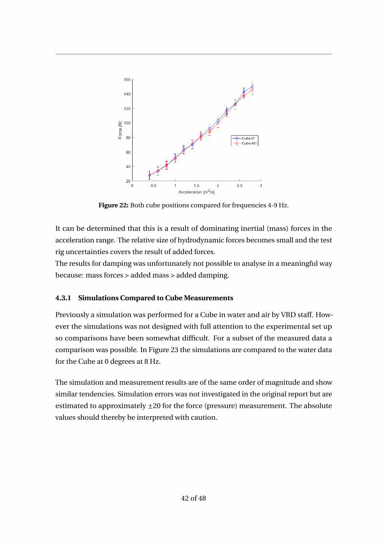
Figure 22: Both cube positions compared for frequencies 4-9 Hz.

It can be determined that this is a result of dominating inertial (mass) forces in the

acceleration range. The relative size of hydrodynamic forces becomes small and the test

rig uncertainties covers the result of added forces.

The results for damping was unfortunately not possible to analyse in a meaningful way

because: mass forces > added mass > added damping.

4.3.1 Simulations Compared to Cube Measurements

Previously a simulation was performed for a Cube in water and air by VRD staff. How-

ever the simulations was not designed with full attention to the experimental set up

so comparisons have been somewhat difficult. For a subset of the measured data a

comparison was possible. In Figure 23 the simulations are compared to the water data

for the Cube at 0 degrees at 8 Hz.

The simulation and measurement results are of the same order of magnitude and show

similar tendencies. Simulation errors was not investigated in the original report but are

estimated to approximately ±20 for the force (pressure) measurement. The absolute

values should thereby be interpreted with caution.

42 of 48

Figure 23: Cube data for 0 degrees at 8 Hz in water compared to simulations in openFOAM.

43 of 48

5 DISCUSSION

This section contains the discussion of uncertainties, added properties, rotor dynamics

and simulations.

5.1 Repeatability and Uncertainties

The measurement devices have quite a wide measuring range. The force range is 100

kg which is quite necessary but the displacement range of 50 mm introduces problems

with relative high uncertainties close to the bottom end of the measurement range. Con-

sidering that the measured displacements are only maximum 6-7% of the measurement

range.

A difficulty with the analysis is the comparison between the water and air tests. The

problem arises when arithmetic calculations are performed with the two data sets. The

forces are similar in size which means that the effect of measurement uncertainties

becomes high relative to the force difference between air and water.

5.2 The Shaker

The shaker must be questioned due to the problems at low frequencies, regulation errors

and random errors. These types of shakers are in general designed to oscillate small

objects at high frequencies. The shaker problems and partly friction has compromised

a large part of the results and complicated the matlab analysis. The really interesting

accelerations close to 0 could not be reached. In the future another shaker option could

be used or a electrodynamic shaker intended for larger loads. To achieve a complete

analysis of added properties with good accuracy this is required.

5.3 Hydrodynamic forces

The hydrodynamic forces are relatively small compared to the inertial force i.e the

moving mass. This means that the difference between water and air test becomes small.

It would be favourable for experimental purposes to increase the relative size of the

hydrodynamic forces, to improve the measurement of added mass and damping. This

could possibly be done by reducing the ratio of object mass to cross-sectional area (in

the direction of motion).

44 of 48

5.3.1 Added Mass

The added mass appears to increase when acceleration decreases. But when will this

increase slow down? When acceleration approaches zero added mass must approach

0% as frequency and vibration amplitude decreases. At very small amplitude or infinite

period time the difference between air and water tests should be zero. Unfortunately

the experimental conditions needed are hard to create with the experimental setup. The

region close to zero is important for dynamics analysis especially when start-up and

shut-down of the machine are considered.

5.3.2 Added Damping

The force associated with maximum object velocity and zero object acceleration called

damping force was throughout the experiments hard to quantify. The magnitude of

damping was small compared to inertia forces and friction so the signal was drowned by

that and other noise for most frequencies. For some of the lower frequencies damping

dominates the force signal but varies a lot. Uncertainties of at best ±30% are seen in

the more favourable situations. Differences between air and water test are found to be

small if any.

5.4 Rotor Dynamics and Simulation Models

The obtained results in there absolute form are not considered directly applicable to

rotor dynamic analysis. This should be seen as a means of verifying numerical models

which then will be used for the scaling to a real prototype simulation. Further, the

data is from simplified experiments with lateral vibrations. A more realistic approach

with a rotating system is needed for a clear determination of the impact off the added

properties. When that work is done it must be determined to which degree the fluid

forces affect the dynamic analysis. Is it a significant contributor to the system response

compared to the other components of the dynamic system?

Simulations could be designed after experimental tests to best replicate the conditions

at the test rig.

45 of 48

6 CONCLUSION

The added mass can be estimated with the test rig when the operations conditions are

favourable. Added mass is estimated in a narrow range because of the test rig limitations.

However the hydrodynamic mass force appears to be function of the acceleration

which is the key parameter in rotor dynamic analysis. The importance of testing many

frequencies and amplitudes must thereby be questioned, compared to the beginning

of the project. The added mass is found to increase for decreasing acceleration and it

is also concluded that added mass is 0 at 0 acceleration. This implies that there is an

added mass maximum which have not been found.

For test object acceleration close to 0 m/s2 the test rig have proved to be insufficient due

to regulation, structural and friction problems. Further the measurement equipment

should be improved to accurately measure the forces and vibrations at low acceleration.

Reliable measurements of added damping have not been possible with the test rig

during the project.

Further research should focus at finding the added mass maxima at low acceleration

and to investigate if it is possible to measure damping in a reliable way. Then a rotating

added mass test rig could be constructed to enable measurements for validation of

numerical models.

46 of 48

REFERENCES

[1] Statistiska centralbyrån, “Årlig energistatistik (el, gas och fjärrvärme):

Eltillförsel i Sverige efter produktionsslag 1986-2015..” http://www.scb.se/hitta-

statistik/statistik-efter-amne/energi/tillforsel-och-an2016.

[2] R.Roman, D.Bucur, J-O.Aidanpää, M.J.Cervantes, “Damping, stiffness and added

mass in hydraulic turbines.” Energiforsk Report 2015:106. ISBN 978-91-7673-106-2,

2016.

[3] C.Trivedi, M.J.Cervantes, “Fluid-structure interactions in Francis turbines: A per-

spective review.” Renewable and Sustainable Energy Reviews 68(2017)87 - 101,

2017.

[4] Rolf Gustavsson, “Rotor Dynamical Modelling and Analysis of Hydropower Units:

Paper F.” Doctoral Thesis: Department of Applied Physics and Mechanical En-

gineering: Division of Computer Aided Design: Luleå Univetsity of Technology:

Sweden, 2008.

[5] Mattias Nässelqvist, “Simulation and Characterization of Rotordynamic Properties

for Vertical Machines.” Doctoral Thesis: Department of Engineering Sciences and

Mathematics: Division of Mechanics and Solid Materials: Luleå Univetsity of

Technology: Sweden, 2011.

[6] G.Krivchenko, “Hydraulic Machines: Turbines and Pumps.” Lewis Publishers sec-

ond edition, 1993.

[7] M.Lindgren, D.Litström, A.Pettersson, M.Sendelius, M.J.Cervantes, “Vägledning för

relativ verknigsgradsmätning med Winter-Kennedymetoden.” Energiforsk Report

2015:123. ISBN 978-91-7673-123-9, 2016.

[8] M.Karlsson, H.Nilsson, J-O.Aidanpää, “Numerical Estimation of Torsional Dynamic

Coefficients of a Hydraulic Turbine.” International Journal of Rotating Machinery.

Volume 2009, ID: 349397, 2009.

[9] M.R.Maxey, J.J.Riley, “Equation of motion for a small rigid sphere in a nonuniform

flow.” The physics of fluids. Volume 26 issue 4, 1983.

[10] N.Salvesen, E.O Tuck, O.Faltinsen, “Ship Motions and Sea Loads.” The society of

naval architects and marine engineers, 1970.

47 of 48

[11] C.E. Brennen, “A review of added mass and fluid inertial forces.” Department of the

Navy - public release, 1982.

[12] C.G.Rodriguez, E.Equsquiza, X.Escaler, Q.W.Liang, F.Avellan, “Experimental inves-

tigation of added mass effects on a Francis turbine runner in still water.” Journal of

Fluids and Structures 22 (2006) 699-712, 2006.

[13] Jakob Hedlund, “Experimental investigation of Hydrodynamic Effects on a Vibra-

tion Kaplan Runner.” Master Thesis: Department of Engineering Sciences and

Mathematics: Luleå Univetsity of Technology: Sweden, 2017.

[14] Stina Bergström, “Added Properties in Kaplan Turine: A Preliminary Investigation.”

Master Thesis: Department of Engineering Sciences and Mathematics: Luleå

Univetsity of Technology: Sweden, 2016.

48 of 48