Embed Size (px)
Citation preview

Experimental Investigation of
Cavitation in a Cylindrical
Orifice
Cameron Stanley
School of Mechanical and Manufacturing Engineering
University of New South Wales
A thesis submitted for the degree of
Doctor of Philosophy
2012


COPYRIGHT STATEMENT
‘I hereby grant the University of New South Wales or its agents the right to
archive and to make available my thesis or dissertation in whole or part in the
University libraries in all forms of media, now or here after known, subject to
the provisions of the Copyright Act 1968. I retain all proprietary rights, such as
patent rights. I also retain the right to use in future works (such as articles or
books) all or part of this thesis or dissertation.
I also authorise University Microfilms to use the 350 word abstract of my
thesis in Dissertation Abstracts International.
I have either used no substantial portions of copyright material in my thesis
or I have obtained permission to use copyright material; where permission has
not been granted I have applied/will apply for a partial restriction of the digital
copy of my thesis or dissertation.’
Signed: . . . . . . . . . . . . . . . . . . . . . . . . . . . . . . . . . . Date: February 15, 2012
AUTHENTICITY STATEMENT
‘I certify that the Library deposit digital copy is a direct equivalent of the final
officially approved version of my thesis. No emendation of content has occurred
and if there are any minor variations in formatting, they are the result of the
conversion to digital format.’
Signed: . . . . . . . . . . . . . . . . . . . . . . . . . . . . . . . . . . Date: February 15, 2012


ORIGINALITY STATEMENT
‘I hereby declare that this submission is my own work and to the best of my
knowledge it contains no materials previously published or written by another
person, or substantial proportions of material which have been accepted for the
award of any other degree or diploma at UNSW or any other educational institu-
tion, except where due acknowledgment is made in the thesis. Any contribution
made to the research by others, with whom I have worked at UNSW or elsewhere,
is explicitly acknowledged in the thesis. I also declare that the intellectual content
of this thesis is the product of my own work, except to the extent that assistance
from others in the project’s design and conception or in style, presentation and
linguistic expression is acknowledged.’
Signed: . . . . . . . . . . . . . . . . . . . . . . . . . . . . . . . . . . Date: February 15, 2012


Acknowledgements
Firstly I would like to gratefully acknowledge the guidance and sup-
port of my supervisors, Associate Professors Gary Rosengarten and
Tracie Barber. Throughout this testing experience they were a con-
stant source of positivity and continually encouraged me to endure
the setbacks and forge ahead. I also thank Emeritus Professor Brian
Milton for his assistance during the various stages of this work.
The completion of this work would not have been possible without the
assistance of the skillful workshop staff in the School of Mechanical
Engineering. I would like to thank Russell Overhall, Ian Cassapi and
Andy Higley for your generous technical advice and support during
the fabrication of the test rig. A special thanks must go to Vince
Carnevale who was always happy to discuss my design concerns and
share his technical wisdom. I truly could not have completed this task
without his assistance.
I would especially like to thank my comrade, cellmate and brother,
Alex Sinclair. Thanks for sharing my office and tolerating me for these
past years. You taught me a lot about engineering, fluid mechanics
and life in general. Without you by my side I may never have made it
to this point and would definitely not have had as many laughs along
the way.
I must also thank my family and close friends whose patience and en-
during support have been greatly appreciated. Finally I would like to
thank my girlfriend Tracey Hollings for her continual encouragement
and positivity.

List of Publications
1. C. Stanley, T. Barber, B. Milton and G. Rosengarten, Periodic
cavitation shedding in a cylindrical orifice, Experiments in Flu-
ids, DOI: 10.1007/s00348-011-1138-7, Available Online (2011)
2. C. Stanley, G. Rosengarten, T. Barber and B. Milton, Investi-
gation of the effects of cavitation on atomization of a high speed
liquid jet, The 5th International Students/Young Birds Seminar
on Multi-scale Flow Dynamics, 4-6 November, Sendai, Japan
(2009)
3. C. Stanley, G. Rosengarten, B. Milton and T. Barber, Investi-
gation of cavitation in a large-scale transparent nozzle, FISITA
World Automotive Congress - Student Congress, F2008-SC-001,
14-19 September, Munich, Germany (2008)

Abstract
The atomisation of liquid jets is of crucial importance to a wide range
of applications including industrial processing, automotive fuel in-
jectors and agriculture. The presence of cavitation in plain orifice
atomisers is known to enhance this process; however the complex flow
mechanisms that result within the nozzle remain incompletely un-
derstood. Periodic cavitation shedding has been widely observed for
external cavitating flows, but has received little attention for nozzle
flows.
A new cavitation research rig was designed and built to facilitate the
investigation of influence of cavitation on atomisation in large-scale
plain orifice nozzles. Refractive index matching with a 8.25mm diam-
eter acrylic nozzle was achieved using aqueous sodium iodide as the
test fluid, which allowed unabated access to the flow structures near
the orifice wall. High-resolution images of the internal flow and near
nozzle spray structures were recorded using high-speed visualisation.
Digital processing was then used to extract cavitation cloud shedding
frequencies, collapse lengths, re-entrant jet motion and spray angles
across a range of Reynolds numbers from 4.8× 10⁴ to 2.2× 10⁵. Noz-
zle discharge coefficient was also measured and revealed an interesting
tendency for the nozzle to revert from the hydraulically flipped state
to supercavitation.
Periodic shedding of cavitation clouds was found to occur for a narrow
range of cavitation numbers corresponding to partial cloud cavitation.
Spectral analysis of the recordings found the frequencies associated
with this shedding to vary linearly with cavitation number, K, from
approximately 500Hz at K = 1.8 to approximately 2500Hz at K =
ix

2.1. Comparison of the shedding behaviour with water revealed strong
agreement. The mechanism behind this periodicity appears to be the
motion of the re-entrant jet, which appears to be largely driven by
the adverse pressure gradient around the flow reattachment zone.
Discontinuities were observed in collapse length and spray angle corre-
sponding to the transition from partial cloud cavitation to developed
cavitation at approximately K = 1.8. It is believed this transition
is related to the slope of the pressure gradient in the stream wise
direction.
Spray angles were shown to be significantly enhanced by the presence
of cavitation in the nozzle with the angle directly related to the dis-
tance of the collapse region to the nozzle exit. Peak angles occur for
supercavitation where the cavitation clouds collapse directly near the
exit plane of the nozzle. Further reductions in cavitation number re-
sulted in transition to the hydraulically flipped state. Transition from
hydraulic flip to supercavitation was regularly observed for cavitation
numbers below K = 1.7. This unusual tendency contravenes typical
jet behaviour and was shown to be related to the vertical inclination
of the nozzle and the disturbance of the separated jet by liquid falling
back down the nozzle under the action of gravity. Discharge coef-
ficient measurements closely follow the 1D model predictions within
the literature except for the region of periodic cavitation shedding. In
this region the presence of cavitation had minimal effect on the nozzle
discharge coefficient, with peak Cd values occurring here.
x

Contents
Abstract . . . . . . . . . . . . . . . . . . . . . . . . . . . . . . . . . . . ix
List of Figures . . . . . . . . . . . . . . . . . . . . . . . . . . . . . . . . xv
List of Tables . . . . . . . . . . . . . . . . . . . . . . . . . . . . . . . . xviii
Nomenclature . . . . . . . . . . . . . . . . . . . . . . . . . . . . . . . . xix
1 Introduction 1
1.1 Background . . . . . . . . . . . . . . . . . . . . . . . . . . . . . . 1
1.2 Atomisation of Liquid Jets . . . . . . . . . . . . . . . . . . . . . . 3
1.3 Cavitation Fundamentals . . . . . . . . . . . . . . . . . . . . . . . 5
1.3.1 Phase Change and Cavitation . . . . . . . . . . . . . . . . 5
1.3.2 Nucleation Theory . . . . . . . . . . . . . . . . . . . . . . 7
1.3.3 Bubble Dynamics and Collapse . . . . . . . . . . . . . . . 8
1.3.4 Cavitating Flows . . . . . . . . . . . . . . . . . . . . . . . 12
1.4 Thesis Outline . . . . . . . . . . . . . . . . . . . . . . . . . . . . . 13
2 Literature Review 15
2.1 Early Studies on Liquid Jet Atomisation . . . . . . . . . . . . . . 15
2.2 The Influence of the Nozzle on Atomisation . . . . . . . . . . . . 16
2.2.1 Effects of Length to Diameter Ratio . . . . . . . . . . . . . 17
2.2.2 Effects of Inlet Rounding . . . . . . . . . . . . . . . . . . . 19
2.2.3 Ambient Conditions . . . . . . . . . . . . . . . . . . . . . 21
2.3 The Effects of Cavitation on Nozzle Flow . . . . . . . . . . . . . . 23
2.3.1 Cavitating Flow Structures . . . . . . . . . . . . . . . . . . 23
2.3.2 Nozzle Turbulence and Jet Breakup . . . . . . . . . . . . . 27
2.3.3 Nozzle Discharge Coefficient . . . . . . . . . . . . . . . . . 30
2.3.4 Injector Specific Observations . . . . . . . . . . . . . . . . 34
xi

CONTENTS
2.4 Periodic Cloud Shedding . . . . . . . . . . . . . . . . . . . . . . . 36
2.4.1 Re-entrant Jet . . . . . . . . . . . . . . . . . . . . . . . . . 37
2.4.2 Shedding Frequency . . . . . . . . . . . . . . . . . . . . . 40
2.5 Summary of the Literature . . . . . . . . . . . . . . . . . . . . . . 42
2.6 Thesis Objectives . . . . . . . . . . . . . . . . . . . . . . . . . . . 43
3 Experimental Rig Design 44
3.1 General Description . . . . . . . . . . . . . . . . . . . . . . . . . . 44
3.2 Test Section . . . . . . . . . . . . . . . . . . . . . . . . . . . . . . 49
3.2.1 Nozzle Design . . . . . . . . . . . . . . . . . . . . . . . . . 49
3.2.2 Analytical Stress Calculations . . . . . . . . . . . . . . . . 52
3.2.3 Finite Element Analysis . . . . . . . . . . . . . . . . . . . 55
3.2.4 Hydrostatic Testing . . . . . . . . . . . . . . . . . . . . . . 57
3.3 Liquid Supply Piping . . . . . . . . . . . . . . . . . . . . . . . . . 58
3.3.1 Flow Development . . . . . . . . . . . . . . . . . . . . . . 58
3.3.2 Computational Fluid Dynamics Modeling . . . . . . . . . . 59
3.4 Hydraulic Actuation System . . . . . . . . . . . . . . . . . . . . . 61
3.5 Optical Access Pressure Vessel . . . . . . . . . . . . . . . . . . . . 65
3.6 Support Frame . . . . . . . . . . . . . . . . . . . . . . . . . . . . 69
3.7 Test Liquid Characterisation -
Sodium Iodide . . . . . . . . . . . . . . . . . . . . . . . . . . . . . 70
3.7.1 Refractive Index Matching . . . . . . . . . . . . . . . . . . 70
3.7.2 Kinematic Viscosity . . . . . . . . . . . . . . . . . . . . . . 73
3.7.3 Density . . . . . . . . . . . . . . . . . . . . . . . . . . . . 74
3.7.4 Vapour Pressure . . . . . . . . . . . . . . . . . . . . . . . 75
3.8 Data Acquisition and Cylinder Control . . . . . . . . . . . . . . . 75
4 Measurement Techniques and Experimental Uncertainty 77
4.1 Data Extraction . . . . . . . . . . . . . . . . . . . . . . . . . . . . 77
4.1.1 Non-dimensional Parameters . . . . . . . . . . . . . . . . . 78
4.2 High-speed Visualisation . . . . . . . . . . . . . . . . . . . . . . . 81
4.2.1 Illumination . . . . . . . . . . . . . . . . . . . . . . . . . . 81
4.2.2 Camera Lens and Region of Interest . . . . . . . . . . . . . 83
4.3 Image Processing Techniques . . . . . . . . . . . . . . . . . . . . . 83
xii

CONTENTS
4.3.1 Cavity Collapse length . . . . . . . . . . . . . . . . . . . . 85
4.3.2 Spray Angle . . . . . . . . . . . . . . . . . . . . . . . . . . 87
4.3.3 Signal Spectral Analysis . . . . . . . . . . . . . . . . . . . 90
4.3.3.1 Power Spectral Density . . . . . . . . . . . . . . 90
4.3.3.2 Calculation Method . . . . . . . . . . . . . . . . 93
4.3.4 Measurement Limitations . . . . . . . . . . . . . . . . . . 95
4.4 Experimental Uncertainty . . . . . . . . . . . . . . . . . . . . . . 96
4.4.1 Analysis Methodology . . . . . . . . . . . . . . . . . . . . 96
4.4.2 Bias Error . . . . . . . . . . . . . . . . . . . . . . . . . . . 97
4.4.3 Precision Error for Single Measurements . . . . . . . . . . 98
4.4.4 Precision Error for Multiple Measurements . . . . . . . . . 98
5 Results and Discussion 101
5.1 Cavitating Flow Regimes . . . . . . . . . . . . . . . . . . . . . . . 101
5.2 Test Parameters . . . . . . . . . . . . . . . . . . . . . . . . . . . . 104
5.3 Collapse Length . . . . . . . . . . . . . . . . . . . . . . . . . . . . 104
5.4 Partial Cavitation . . . . . . . . . . . . . . . . . . . . . . . . . . . 110
5.4.1 Periodic Cloud Shedding . . . . . . . . . . . . . . . . . . . 110
5.4.2 Re-entrant Jet . . . . . . . . . . . . . . . . . . . . . . . . . 111
5.4.2.1 Re-entrant Jet Motion . . . . . . . . . . . . . . . 113
5.4.2.2 Estimation of Re-entrant Jet Velocity . . . . . . . 117
5.4.2.3 Asymmetric Cloud Shedding . . . . . . . . . . . 121
5.4.3 Measurement of Periodic Shedding Frequencies . . . . . . . 124
5.5 Developed Cavitation . . . . . . . . . . . . . . . . . . . . . . . . . 128
5.5.1 Cavity Appearance . . . . . . . . . . . . . . . . . . . . . . 128
5.5.2 Transient Motion of Closure Region . . . . . . . . . . . . . 129
5.5.3 Sublayer Motion . . . . . . . . . . . . . . . . . . . . . . . 131
5.6 Nozzle Discharge Coefficient . . . . . . . . . . . . . . . . . . . . . 131
5.6.1 Comparison to 1-dimensional theory . . . . . . . . . . . . 133
5.6.2 Transition from Hydraulic Flip to Supercavitation . . . . . 135
5.7 Near-Nozzle Spray Structure Visualisation . . . . . . . . . . . . . 137
5.7.1 Spray Surface Appearance . . . . . . . . . . . . . . . . . . 137
5.7.2 Measurements of Spray Angle Variation with Cavitation . 139
xiii

CONTENTS
5.7.3 Ligament and Droplet Formation . . . . . . . . . . . . . . 141
6 Conclusions and Recommendations 144
6.1 Key Findings . . . . . . . . . . . . . . . . . . . . . . . . . . . . . 144
6.2 Recommendations for Future Work . . . . . . . . . . . . . . . . . 146
A Uncertainty Analysis 148
B Instrumentation Calibration 173
C Pressure Vessel Drawings 178
D Hydraulic Equipment 189
References 192
xiv

List of Figures
1.1 Common diesel fuel injector geometry . . . . . . . . . . . . . . . . 2
1.2 Typical phase change diagrams . . . . . . . . . . . . . . . . . . . 6
1.3 Heterogeneous nucleation formed from a crevice . . . . . . . . . . 8
1.4 Micro-bubble in equilibrium . . . . . . . . . . . . . . . . . . . . . 9
1.5 Equilibrium of a spherical bubble . . . . . . . . . . . . . . . . . . 10
2.1 Sharp-edged and rounded inlet nozzle producing the same spray
angle . . . . . . . . . . . . . . . . . . . . . . . . . . . . . . . . . . 19
2.2 Droplet size dependence on mean flow velocity . . . . . . . . . . . 20
2.3 Breakup length stability curve . . . . . . . . . . . . . . . . . . . . 23
2.4 Plug Cavitation . . . . . . . . . . . . . . . . . . . . . . . . . . . . 25
2.5 One-dimensional cavitating nozzle flow . . . . . . . . . . . . . . . 31
2.6 Compilation of experimental nozzle discharge coefficient . . . . . . 33
2.7 Schematic representation of the re-entrant jet formation . . . . . . 37
3.1 Experimental rig schematic . . . . . . . . . . . . . . . . . . . . . . 45
3.2 Overall view showing pressure vessel and support frame . . . . . . 47
3.3 Hydraulic and test fluid cylinder configuration . . . . . . . . . . . 48
3.4 Acrylic test piece . . . . . . . . . . . . . . . . . . . . . . . . . . . 51
3.5 Stress calculations cross-sectional area . . . . . . . . . . . . . . . 53
3.6 Finite Element Analysis stress calculations . . . . . . . . . . . . . 56
3.7 Nozzle supply-pipe centerline dimensions . . . . . . . . . . . . . . 60
3.8 Cross-section of CFD pipe mesh . . . . . . . . . . . . . . . . . . . 61
3.9 Secondary velocity fields . . . . . . . . . . . . . . . . . . . . . . . 62
3.10 CFD velocity profiles . . . . . . . . . . . . . . . . . . . . . . . . . 63
xv

LIST OF FIGURES
3.11 Pressure vessel . . . . . . . . . . . . . . . . . . . . . . . . . . . . 66
3.12 Pressure vessel and test section configurations . . . . . . . . . . . 68
3.13 Experimental refractive index matching . . . . . . . . . . . . . . . 72
3.14 NaI kinematic viscosity regression . . . . . . . . . . . . . . . . . . 73
3.15 NaI density as a function of solution concentration . . . . . . . . . 74
3.16 NaI vapour pressure as a function of temperature . . . . . . . . . 75
4.1 Pressure trace . . . . . . . . . . . . . . . . . . . . . . . . . . . . . 79
4.2 Schematic of near-nozzle spray visualisation setup . . . . . . . . . 82
4.3 Schematic of visualisation region of interest . . . . . . . . . . . . . 84
4.4 Collapse length image processing . . . . . . . . . . . . . . . . . . 86
4.5 Spray images for Re = 6.5× 10⁴ and K = 1.83 . . . . . . . . . . . 88
4.6 Spray angle definition - right side shown . . . . . . . . . . . . . . 89
4.7 Schematic of the signal segmentation using Welch’s averaged peri-
odogram . . . . . . . . . . . . . . . . . . . . . . . . . . . . . . . . 92
4.8 Schematic of interrogation spots used for cavitation frequency anal-
ysis . . . . . . . . . . . . . . . . . . . . . . . . . . . . . . . . . . . 94
5.1 Representative nozzle cavitation structures . . . . . . . . . . . . . 102
5.2 Time-averaged, normalised cavitation collapse length . . . . . . . 106
5.3 Cavitation collapse length comparison . . . . . . . . . . . . . . . . 108
5.4 Periodic cavitation shedding sequence . . . . . . . . . . . . . . . . 112
5.5 Cavitation shedding sequence showing detailed re-entrant jet motion114
5.6 Schematic illustration of typical re-entrant jet motion . . . . . . . 116
5.7 Re-entrant jet interface deformation image sequence . . . . . . . . 118
5.8 Re-entrant jet interface tracking . . . . . . . . . . . . . . . . . . . 118
5.9 Ratio of re-entrant jet travelling wave velocity, Vj to mean nozzle
velocity, Vn . . . . . . . . . . . . . . . . . . . . . . . . . . . . . . 120
5.10 Bubble motion in the re-entrant . . . . . . . . . . . . . . . . . . . 121
5.11 Image sequence showing asymmetric motion of re-entrant jet . . . 123
5.12 Power spectral density analysis . . . . . . . . . . . . . . . . . . . 125
5.14 Turbulent reattachment with sporadic cavitation shedding, K =
1.79, Re = 6.9× 10⁴ . . . . . . . . . . . . . . . . . . . . . . . . . 129
5.15 Power spectral density analysis . . . . . . . . . . . . . . . . . . . 130
xvi

LIST OF FIGURES
5.16 Nozzle discharge coefficient as a function of cavitation number . . 132
5.17 Discharge coefficient for partial cavitation . . . . . . . . . . . . . 134
5.18 Pressure data showing fluctuations between hydraulic flip and su-
percavitation . . . . . . . . . . . . . . . . . . . . . . . . . . . . . 136
5.19 Nozzle discharge coefficient comparison from early injection to late 137
5.20 Representative images of spray structure . . . . . . . . . . . . . . 138
5.21 Near nozzle spray angle as a function of cavitation number . . . . 140
5.22 Ligament formations sequence for partial and supercavitation . . . 142
B.1 Pressure vessel gas pressure sensor calibration . . . . . . . . . . . 174
B.2 Injection pressure sensor calibration . . . . . . . . . . . . . . . . . 174
B.3 Gas temperature thermocouple calibration . . . . . . . . . . . . . 175
B.4 Liquid temperature thermocouple calibration . . . . . . . . . . . . 175
B.5 LDT piston position calibration . . . . . . . . . . . . . . . . . . . 176
B.6 Piston velocity calibration . . . . . . . . . . . . . . . . . . . . . . 177
C.1 Pressure vessel - drawing sheet 1 . . . . . . . . . . . . . . . . . . 179
C.2 Pressure vessel - drawing sheet 2 . . . . . . . . . . . . . . . . . . 180
C.3 Pressure vessel - drawing sheet 3 . . . . . . . . . . . . . . . . . . 181
C.4 Pressure vessel - drawing sheet 4 . . . . . . . . . . . . . . . . . . 182
C.5 Pressure vessel - drawing sheet 5 . . . . . . . . . . . . . . . . . . 183
C.6 Pressure vessel - drawing sheet 6 . . . . . . . . . . . . . . . . . . 184
C.7 Pressure vessel - drawing sheet 7 . . . . . . . . . . . . . . . . . . 185
C.8 Pressure vessel - drawing sheet 8 . . . . . . . . . . . . . . . . . . 186
C.9 Pressure vessel - drawing sheet 9 . . . . . . . . . . . . . . . . . . 187
C.10 Pressure vessel - drawing sheet 10 . . . . . . . . . . . . . . . . . . 188
D.1 Hydraulic System Schematic . . . . . . . . . . . . . . . . . . . . . 190
D.2 Test Fluid Cylinder End Cap . . . . . . . . . . . . . . . . . . . . 191
xvii
List of Tables
3.1 Experimental rig schematic component list . . . . . . . . . . . . . 46
3.2 Nozzle Parameters . . . . . . . . . . . . . . . . . . . . . . . . . . 50
3.3 Material Properties of Cast Acrylic . . . . . . . . . . . . . . . . . 52
3.4 Analytical nozzle stresses . . . . . . . . . . . . . . . . . . . . . . . 55
3.5 FEA nozzle stresses . . . . . . . . . . . . . . . . . . . . . . . . . . 57
3.6 Pressure vessel design parameters . . . . . . . . . . . . . . . . . . 67
3.7 Pressure vessel assembly component list . . . . . . . . . . . . . . 69
3.8 Physical Properties of Aqueous Sodium Iodide . . . . . . . . . . . 76
4.1 Measurement parameters and estimated uncertainties . . . . . . . 100
5.1 Experimental Parameters . . . . . . . . . . . . . . . . . . . . . . . 105
5.2 Measured re-entrant jet velocity for various conditions . . . . . . . 119
xviii

Nomenclature
Roman Symbols
∆z vertical height difference
mact actual mass flow rate
mth theoretical mass flow rate
SAV PER averaged periodogram power spectral density estimator
SPER periodogram power spectral density estimator
SW Welch’s averaged power spectral density estimator
A nozzle cross-sectional area
C sodium iodide concentration
Cc contraction coefficient
Cd discharge coefficient
Cv velocity coefficient
Dc test fluid cylinder bore diameter
Dn nozzle diameter
Dp supply pipe diameter
f frequency
xix
NOMENCLATURE
fs sampling frequency
g gravitational constant
K cavitation number
L nozzle length
L/D nozzle length to diameter ratio
Lcav cavity length
Lcav/L dimensionless cavity collapse length
P static pressure
P1 nozzle injection pressure
P2 ambient gas pressure
Pg partial pressure of gas
Pv vapour pressure
PgO initial gas partial pressure
R bubble radius
r radial variable
r/R nozzle inlet rounding to nozzle radius ratio
Rc critical bubble radius
ri inner radius
RO initial bubble radius
ro outer radius
Rsp supply pipe bend curvature radius
Re Reynolds number
xx

NOMENCLATURE
S liquid surface tension
SXX power spectral density
T Temperature
U data window power scaling factor
V velocity
Vc piston velocity
Vj re-entrant jet velocity
Vn average nozzle velocity
Vo LDT output voltage
V∞ free-stream velocity
Vliq liquid velocity within re-entrant jet
Vnththeoretical nozzle velocity
w(n) data window
We Weber number
x stream-wise co-ordinate
xp piston axial position
xLL spray angle analysis - lower left gas/liquid interface position
xLU spray angle analysis - upper left gas/liquid interface position
xRL spray angle analysis - lower right gas/liquid interface position
xRU spray angle analysis - upper right gas/liquid interface position
yLL spray angle analysis - vertical lower-limit
yL spray angle analysis - vertical position of lower gas/liquid interface
xxi

NOMENCLATURE
yUL spray angle analysis - vertical upper-limit
yU spray angle analysis - vertical position of upper gas/liquid interface
Greek Symbols
µ dynamic viscosity
ν kinematic viscosity
νp Poisson’s ratio
ρ density
σ traditional cavitation number
σa axial stress
σh hoop stress
σr radial stress
σy tensile yield strength
θ spray angle
θL left-side spray angle
θR right-side spray angle
Acronyms
ANSI American National Standards Institute
CFD Computational Fluid Dynamics
CI Compression Ignition
CMOS Complementary MetalOxideSemiconductor
CR Contraction Ratio
DTFT Discrete-Time Fourier Transform
xxii

NOMENCLATURE
FEA Finite Element Analysis
fps Frames Per Second
FSO Full Scale Output
LDA Laser Doppler Anemometry
LDT Linear Displacement Transducer
LDV Laser Doppler Velocimetry
PIV Particle Image Velocimetry
PMMA Polymethyl Methacrylate - “Acrylic”
PSD Power Spectral Density
R− P Rayleigh-Plesset Equation
ROI Region Of Interest
TKE Turbulent Kinetic Energy
V CO Valve Covered Orifice
V OF Volume Of Fluid
xxiii

Chapter 1
Introduction
1.1 Background
The atomisation of liquid jets is of central importance to a wide range of applica-
tions including industrial processing, automotive fuel injectors and agriculture. In
essence, the process of atomisation involves the conversion of a liquid jet or sheet
into a dispersed spray of small droplets within a gaseous environment (Lefebvre
(1989)). The physical devices used to produce these sprays are generally termed
atomisers or nozzles. Regardless of the method of atomisation, there are a num-
ber of key elements which influence the process, such as the hydraulics of the
internal nozzle flow, the generation of liquid turbulence and the aerodynamic in-
teraction of the jet with the gaseous medium. Each of these factors, together
with the physical properties of the liquid and gas, has a marked influence on
determining the shape and distribution of the final spray.
Combustion engines are heavily reliant on the effective atomisation of liquid
fuels by the injector nozzle to produce a distribution of small droplets within the
combustion chamber. The creation of small droplets of liquid fuel dramatically
increases the surface area of the fuel, which promotes mixing and evaporation.
This process is particularly important for diesel engines where fuel injection is
the most important parameter affecting engine performance. In fact, the com-
bustion efficiency and emission products of compression ignition (CI) engines are
widely known to depend strongly upon the effectiveness of this process (Giffen &
Muraszew (1953)).
1

1.1 Background
Plain-orifice atomisers are a type of pressure atomiser which utilise a cylin-
drical contraction to increase the liquid velocity and generate jet breakup. The
design of a typical diesel fuel injector incorporates multiple plain-orifice style noz-
zles due primarily to their simplicity, durability and relative ease of manufacture.
A schematic showing basic diesel injector nozzle geometries can be seen in figure
1.1.
Plain-orifice
Needle Needle
Figure 1.1: Common diesel fuel injector geometry for a mini-sac injector (left)
and VCO injector (right). Both styles use a plain-orifice to atomise the liquid
fuel. Image is modified from Bae et al. (2002).
The high velocities generated by the contraction cause a reduction of the static
pressure within the nozzle and can subsequently result in cavitation. The presence
of cavitation in the nozzle has been shown to have dramatic influence on the
atomisation. Turbulence generated by the collapse of cavitation bubbles increases
the disruption of the surface of the jet and helps overcome the consolidating force
of surface tension. While this is advantageous to the atomisation process the
cavitation collapse can also be highly destructive and may result in material
degradation or ultimately failure of the injector.
The progressive introduction of increasingly stringent emissions standards for
automobiles has reinforced the importance of improving the atomisation process
2

1.2 Atomisation of Liquid Jets
for diesel fuel injectors. Enhancements to current injector designs are under-
pinned by a need to further our understanding of the fundamental physics af-
fecting the atomisation process. Owing to the complexity of the fluid mechanics
involved, the exact mechanisms for the improvements to atomisation due to cavi-
tation are not fully understood. However, experimental studies on real-sized fuel
injector nozzle are very difficult due to the high velocities, high pressures and
small physical scales. To overcome some of these limitations large scale replica
nozzles are commonly used which significantly enhances the ability to conduct ex-
perimental investigations. Scaling the effects of cavitation between the large-scale
replica nozzles and the real scale cannot be truly achieved due to the fundamental
timescales associated with the bubble behaviour. Despite this obvious constraint
large scale nozzle experiments have demonstrated very similar flow structures to
small cavitating nozzles and offer dramatic improvements to the optical resolu-
tion of the cavitation phenomena. Complementary to the direct improvements
to the understanding of the fundamental physics, experimental data obtained in
large-scale orifice studies can also be valuable for the development and validation
of cavitation models (Gavaises et al. (2009)). Regardless of efforts to downsize
engines size and moves towards electric vehicles the social and economic inertia to
change look certain to ensure diesel engines remain as a widespread transporta-
tion power supply for the foreseeable future. Irrespective of the alternatives,
it is pertinent to continue efforts to improve the combustion efficiency and fuel
economy of diesel engines.
1.2 Atomisation of Liquid Jets
Despite the importance and wide ranging applications of atomisation, a universal
definition is rather elusive. Generally speaking the process involves the breakdown
of a cohesive liquid jet into much smaller droplets. In fact the root word atom is
perhaps a little misleading, as the dimensional scale of the droplets produced are
many orders of magnitude larger. However, the connotation implies the desired
outcome is a dispersion of very small droplets of the liquid phase in a continuous
gaseous medium. Sprays can be produced in a variety of ways and essentially all
that is required to achieve this breakdown is a high relative velocity between the
3
1.2 Atomisation of Liquid Jets
liquid and the surrounding gas. There are a number of different styles of atomiser
which can achieve this aim including plain orifice, swirl, pintle and air blast.
Each of these have certain capabilities and limitations which lend themselves
to particular applications. Plain orifice atomisers, of interest to this work, are
perhaps the most basic of all atomisers. They utilise a reduction of flow area to
generate high liquid velocities. Typically the smaller the orifice the the higher
the liquid velocity the finer the droplet size produced.
In the study of atomising nozzles, atomisation is generally regarded as the
condition whereby a liquid jet is broken up into droplets directly upon exiting
the nozzle. In general the breakup of a liquid jet requires interaction with the
gaseous medium, and so occurs over a finite length. A distance referred to as the
breakup length is used to describe the stream-wise penetration of the spray from
the nozzle exit until the jet is regarded as “atomised”. Generally this refers to
the point where the solid liquid core has been broken into an array of smaller
droplets by the interaction of aerodynamic shear forces. It is often difficult to
establish this location, and often the technique used is highly dependent on the
experimental conditions. The break-up length of a fuel spray in a high speed
small direct injection diesel engine may be of the order of the distance between
the injector and the combustion chamber wall. For this reason, the break-up
length has a very important role in the spatial distribution of liquid fuel and also
on the air-fuel ratio (Hiroyasu (1991)).
The mechanism by which the jet is physically broken into droplets is extremely
complex and highly dependent on the liquid properties and flow conditions. Typ-
ically, for high velocity turbulent jet atomisation, perturbations are produced on
the surface of the jet by turbulence, inertial effects or velocity profile relaxation.
Once formed these perturbations are acted upon by aerodynamic shear forces and
amplified. Eventually the disruptions to the surface structure protrude out later-
ally and get disintegrated into droplets by surface tension, in a process referred to
as primary atomisation. For low enough relative velocities the cohesive force of
viscosity allows the initial perturbations to form extended “finger-like” columns
of liquid, known as ligaments. These ligaments, and any large droplets formed
during the primary atomisation continue to be broken up due to the deforma-
4

1.3 Cavitation Fundamentals
tion of the droplet resulting from aerodynamic interaction, which is referred to
as secondary atomisation.
The improvements to the atomisation process due to cavitation is generally at-
tributed to the increased levels of turbulence created by the explosive growth and
collapse of cavitation bubbles within the orifice. Increased turbulence strengthens
the lateral velocity fluctuations and tends to increase the size of the surface per-
turbations, which promotes aerodynamic interaction. Experiments have shown
the enhancements to atomisation improve as the proximity of the cavitation col-
lapse region nears the nozzle. However, the collapse of bubbles, particularly in
highly turbulent flow fields, is extremely complex. As such the exact mechanism
linking the bubble collapse with the improvements of atomisation are not well
understood. Particularly, characterising the influence of complex cavitating flow
structures, such as periodic cavitation, have received little attention.
1.3 Cavitation Fundamentals
In simple terms, cavitation describes the change of phase from liquid to gas due to
the reduction of pressure. At a low enough pressure, the originally homogeneous
liquid medium will rupture and produce vapour, which can occur for cases where
the liquid is both static and in motion. The type of cavitation of relevance to this
thesis is known as hydrodynamic cavitation, which relates to cavitation occurring
in flowing liquids.
The following sections provide a brief introduction to some of the fundamen-
tals of the cavitation phenomenon. It is in no way exhaustive, but rather is
intended as a refresher to some of the basic theory required to understand the
physics of the cavitating flows described in this thesis. For comprehensive reviews
of cavitation the reader can refer to Knapp et al. (1970), Brennen (1995) or Franc
& Michel (2004).
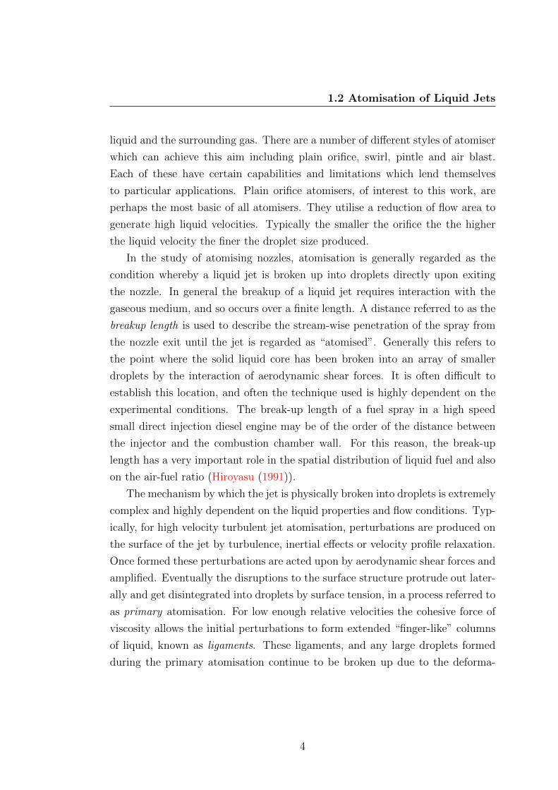
1.3.1 Phase Change and Cavitation
Generally in considering the change of phase from liquid to gas, reference is made
to a typical phase diagram, as shown in figure 1.2. For pure substances such
5
1.3 Cavitation Fundamentals
as water, the triple point is separated from the critical point by the saturated
liquid/vapour line. Crossing this line represents a change of phase between liq-
uid and gas. The process of cavitation and boiling are shown to demonstrate
two such processes and illustrate the fundamental differences between the two.
Boiling is the process of vapour formation due to the addition of heat at approx-
imately constant pressure whereas cavitation is the formation of vapour due to
the reduction of pressure at approximately constant temperature. In the case of
hydrodynamic cavitation the reduction of pressure required for the phase change
is due to localised high velocities caused, for example, by geometric constrictions.
P
T
Critical Point
Triple Point
SOLID LIQUID
VAPOUR
Boiling
Cavitation
SAT. LIQ/VAPPv(T)
P
V
Pv(T)
0
VAPOUR
VAPOUR/
LIQUID
Critical PointLIQUID
Theoretical Isotherm
A
B C
E
D
Figure 1.2: Typical phase change diagrams
Generally the transformation from liquid to vapour phase is thought to occur
at the vapour pressure of the liquid, Pv(T ) . This process is illustrated as the
horizontal passage from point B to point C in the P-V diagram on the right of
figure 1.2. In most practical situations and in the presence of sufficient bubble
nucleation sites this is the case. However, other isotherms between the liquid
and vapour state are possible. In the absence of nucleation sites a liquid may
transition to vapour through “metastable” points, withstanding pressures below
the vapour pressure without rupture. In fact, it is possible for the pressure to fall
below absolute zero, at which point the liquid is under tension. Point E along the
6

1.3 Cavitation Fundamentals
theoretical isotherm shown represents a state of dynamic equilibrium whereby the
liquid is experiencing tension. The presence of any localised impurities will lead
to rupture and a transition to state D. Estimates derived from van der Waals
equation of state indicate pure liquids are capable of withstanding tensions of
around 500 atmospheres at room temperature. These enormous values have never
been achieved experimentally, as invariably liquids contain local weaknesses which
allow the fluid to rupture well before these limits are reached. These weaknesses
are referred to as nucleation points.
1.3.2 Nucleation Theory
Nucleation is generally classified as either homogeneous or heterogeneous. Homo-
geneous nucleation is the generation of momentary microscopic voids in the bulk
of the fluid due to thermal motion. It produces widespread and uniform vapour
production. Alternatively, heterogeneous nucleation describes the formation of
localised weakness within the flow which lead to liquid rupture. There are a num-
ber of sources of heterogeneous nucleation including “free-stream” nuclei created
either by micro-bubbles of dissolved gases or microscopic contaminant particles,
and “surface nuclei” which consist of gas caught in microscopic crevices of the
boundary walls or guiding body which are not completely filled by the liquid.
Typically, conical crevices such as shown in figure 1.3 are considered to exemplify
the surface nucleation points created from such roughness topology (Brennen
(1995)). As liquid pressure in the vicinity of these nucleation sites is reduced,
the cavity expands allowing the generation and release of vapour bubbles into the
bulk of the liquid.
Nuclei can also be produced by cavitation itself, particularly in the cloud
cavitation regime. Each of these nucleation sites provide specific locations where
the fluid can rupture when the pressure is reduced to the vapour pressure. In most
practical engineering environments, heterogeneous nucleation will predominate.
Different levels of nucleation can significantly alter the observed cavitation
structures. Observations of cavitation inception are particularly sensitive to the
variations in the nucleation population, which have been shown to be the origin of
discrepancies when tests on similar bodies were made at different facilities (Franc
7

1.3 Cavitation Fundamentals
θ
2α
Bubble
Liquid
Wallθ
2αBubble
Liquid
Wall
Hydrophilic surface Hydrophobic surface
Figure 1.3: Heterogeneous nucleation formed from a crevice
& Michel (2004)). Quantification of the free-stream nuclei population within a
liquid body is rather difficult, but a distribution of the nuclei number density
can be measured with acoustic and optical techniques. Perhaps the most reliable
methods for quantification of the nuclei present involves taking a holograph of
the liquid and reconstructing the field to inspect the nuclei. A summary of the
numerous methods employed at different research facilities was presented by Billet
(1985). In general surface nuclei cannot be measured, but can be controlled to
some degree by careful attention to the surface finish of the device.
1.3.3 Bubble Dynamics and Collapse
Interesting observations on the growth and stability of cavitation bubbles can be
gained from considering the behaviour of an isolated spherical bubble in equi-
librium with the surrounding liquid, shown in figure 1.4. The complete analysis
will not be repeated here for brevity. For practical situations the bubble can be
expected to contain both liquid vapour and dissolved gas. In this case a force
balance yields;
P = Pg + Pv −2S
R(1.1)
8

1.3 Cavitation Fundamentals
R
P
Pv + Pg
Figure 1.4: Micro-bubble in equilibrium
where R is the bubble radius, Pv is the vapour pressure, Pg is the partial pressure
of the gas and S is the surface tension. If we now consider the action of such
a bubble as it experiences an isothermal change in the external pressure field,
ignoring gas diffusion and assuming the surface remains spherical. It is possible
to re-write the equation 1.1 in terms of initial conditions so that the effects of
changes in the pressure field can be predicted for different nuclei. For isother-
mal pressure variations the gas pressure within the nuclei is proportional to the
volume, yielding the following expression;
P = Pg0
[R0
R
]3
+ Pv −2S
R(1.2)
where the subscript 0 refers to initial conditions for both the nuclei radius and gas
pressure. There are two counteracting forces at play on the bubble; the internal
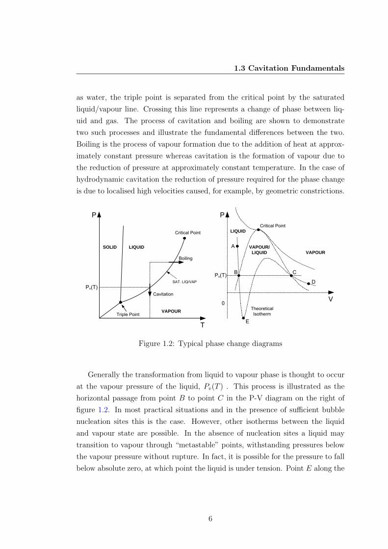
pressure force tending to increase the bubble size, and the surface restoring surface
tension force. Differentiating equation 1.2 yields the minimum or critical bubble
radius, Rc, for the given initial conditions. Figure 1.5 is a plot showing a number
of these equilibrium curves. As the pressure is reduced the bubble will expand.
Provided the expansion produces a bubble radius less than the critical size, then
the balance of forces will return the nuclei to its initial size. In other words, the
mechanical equilibrium for the bubble on the branch of the curve to the left of
the critical radius is stable. For pressure reductions beyond the critical pressure,
the bubble is no longer stable and will grow explosively.
9
1.3 Cavitation Fundamentals
R2,0
P
P,0
Rc
R1,0
Pv
Pc
R0
Stable Region
Unstable Region
locus of minima
Figure 1.5: Equilibrium of a spherical bubble
The pressure difference between the vapour pressure and critical pressure is
known as the static delay of cavitation. Importantly, the static delay is always
positive and gets larger for smaller nuclei. However this analysis is highly simpli-
fied and provides a representational understanding of the influences of pressure
reduction on the nuclei present in the liquid. Real fluids will contain a distribu-
tion of nuclei sizes. When subjected to low pressure some of these nuclei will be
sufficiently small that they remain passive. Others may be large enough that the
pressure will initiate violent expansion.
The applicability of this simplified quasi-static analysis is limited to situations
where the time spent in the low-pressure region is long compared to the collapse
time of the bubble. For longer time periods diffusion of dissolved gases can affect
the growth. For shorter growth cycles inertial and viscous effects can become
influential.
The dynamic response of spherical nuclei is somewhat more complex. The
most common equation of motion is the Rayleigh-Plesset (R-P) equation;
10

1.3 Cavitation Fundamentals
ρ
[RR +
3
2R2
]= Pv − P∞(t) + Pg0
[R0
R
]3
− 2S
R− 4µ
R
R(1.3)
In its earliest form the equation, derived by Rayleigh (1917), described the col-
lapse of spherical bubbles modelled as voids in an infinite homogeneous incom-
pressible liquid field. His work was later continued by Plesset (1949) to account
for surface tension and vapour pressure within the bubble, which eliminated the
infinite velocities of bubble collapse predicted by Rayleigh’s model. The effects
of contaminant gases on the bubble dynamics were later added. It is common for
only the linear term in the full R-P equation to be used for increased numerical
stability.
A detailed analysis of the bubble motion described by the R-P equation is
beyond the scope of this work, although a few important points are worthy of
noting. The non-linear nature of equation 1.3 alludes to the complexity of the
bubble motion it describes. Attempts to numerically model the motion often
make simplifying assumptions which ignore certain influences such as viscosity
or surface tension. In doing so, they modify the true behaviour of the bubble.
However, they do exhibit the main features of bubble growth and collapse, some
of which can be summarised as follows:
• Bubble growth is fairly smooth, with the maximum bubble size occurring
after the region of lowest pressure. Bubble collapse is catastrophic occurring
over very short periods of time.
• During collapse the interface accelerates as the radius of the bubble reduces
reaching extremely high collapse velocities which can exceed 1000m/s. Suc-
cessive rebound and collapse cycles occur, which are dissipated by viscosity.
The actual growth and collapse of nuclei in cavitating devices is complicated
further by turbulence and non-uniform pressure fields.
• An imbalance in the forces acting on the surface of bubbles can create
asymmetric collapse. This promotes the formation of a liquid jet which is
accelerated by the collapse and can impact the back of the bubble with
11

1.3 Cavitation Fundamentals
extremely high velocity. The impact of this water jet can cause significant
damage when the asymmetric collapse occurs in the proximity of a surface.
1.3.4 Cavitating Flows
There are a number of different types of cavitating flow structures that form in
hydrodynamics. Cavitating flows are almost invariably complex and varied but
can be broadly classified based on the overall appearance and effects on the flow
of the cavitation structures.
Bubble Cavitation - describes the formation and collapse of discrete vapour
bubbles within low pressure regions of the flow. It is perhaps the simplest form
of cavitation and is highly dependent on the nuclei size and distribution within
the fluid, or the entrainment of nuclei from solid surfaces. Bubble collapse is
characterised as being violent, noisy and can be highly destructive.
Sheet/Attached Cavitation - refers to cavitation structures which form at fixed
locations, typically due to the low pressure regions created by the dynamic flow
interaction with a solid body or obstacle. Often the cavitation structures occupy
a flow recirculation zone and form large coherent cavities, the surface appearance
of which is dependent on the upstream boundary layer flow. The cavity closure
region is highly complex and large scale instabilities can result.
Partial Cavitation - is a type of sheet cavitation for which the cavity closure
occurs on or within the body to which it is attached.
Supercavitation - is also a type of sheet cavitation. In studies of cavitation
on hydrofoils, supercavitation refers to the situation where cavity closure occurs
downstream from the trailing edge. Specifically, for cavitation in orifices, super-
cavitation refers to the condition where cavity closure occurs at or just past the
exit plane of the orifice/nozzle.
Cloud Cavitation - is a form of partial cavitation which occurs when instabili-
ties result in large-scale shedding of clusters of bubbles which appear as “clouds”.
The coherent collapse of these structures can produce localised shock waves within
the liquid. Following the collapse small bubbles of non-condensible gases remain,
providing a source of nuclei for further cavitation events.
12

1.4 Thesis Outline
The propensity for the occurrence of cavitation within a liquid is described
by a non-dimensional parameter called the cavitation number. In traditional
cavitation studies it is defined as;
σ =P∞ − Pv
12ρV 2∞
(1.4)
and it relates the static pressure tending to suppress cavitation, to the dy-
namic pressure tending to promote it. However, there have been a number of
alternative cavitation numbers proposed and used extensively in the study of
cavitation orifices. Generally they are expressed in terms of the static pressures
as they are easy to measure. The cavitation number used in this work is that
used by Nurick (1976) which is defined as;
K =P1 − PvP1 − P2
. (1.5)
where P1 is the injection pressure and P2 is the ambient gas pressure. As the
cavitation number is reduced the flow conditions become more conducive to cav-
itation. It can be easily observed that this tendency is produced by increases
in injection pressure, P1, or a decrease in the ambient gas pressure, P2. Con-
versely, reductions in injection pressure or increases in back pressure suppress the
tendency for a nozzle to cavitate and result in increases in the cavitation number.
1.4 Thesis Outline
This thesis aims to provide a fundamental study of the effects of cavitation on
orifice flow. It is a step back from the geometric specific applications of plain
orifice atomisers such as diesel injectors but it serves to improve the understanding
of the flow physics at play. As will be seen in Chapter 2, a substantial portion
of the literature concerning cavitation in orifices is motivated by applications to
fuel injector nozzles. However, the applications for cavitation orifices are more
widespread. The aim of this research, while being motivated by diesel injector
flows, is to carry out a fundamental investigation of the influence of cavitation
on orifice flows.
13

1.4 Thesis Outline
The outline of this thesis is as follows. Chapter 2 provides a thorough review of
the literature relating to cavitation in orifices. Attention is given to demonstrating
the application of such flows to the atomisation of liquid jets. Chapter 3 provides
a thorough description of the design and development of the experimental rig
used for this study. As the design was complex and incorporated significant
engineering considerations it will be discussed in detail. This study also uses a
refractive index matching technique to improve the fidelity of the results. The
characterisation of the fluid used for this will also be covered in this chapter.
Chapter 4 describes the measurement and analysis techniques employed in this
study. It also discusses the sources of measurement uncertainty within the work.
Chapter 5 presents the results obtained in the study. A number of fundamental
aspects of cavitation within an orifice are explored in detail. Finally Chapter 6
provides some conclusions obtained from the study and identifies possible future
work. A comprehensive breakdown of the error analysis is presented in Appendix
A, providing details of the elemental sources of error for the measurement of
experimental parameters. Calibration curves for relevant measurements devices
is then presented in Appendix B. Appendix C presents the engineering drawings
of an optical access pressure vessel designed as part of this study. Appendix D
presents schematics of the hydraulic circuitry presented in Chapter 3.
14

Chapter 2
Literature Review
2.1 Early Studies on Liquid Jet Atomisation
The breakup of liquid jets is crucial to a wide range of applications and has been a
topic of research since the late nineteenth century. Early work by Plateau (1945)
demonstrated the breakup of a cylindrical liquid column under the action of
surface tension forces once its length exceeded its perimeter. Rayleigh (1917) used
linear stability analysis to demonstrate that infinitesimal surface perturbations
could rapidly grow and breakup low velocity invisid liquid jets. Weber (1931)
extended the work of Rayleigh to include viscosity and aerodynamic interaction.
However, significant work on the breakup of high speed jets, which is relevant to
the work of this thesis, did not begin in earnest until the 1920’s and 1930’s. Driven
mainly by a need to increase the efficiency of solid1 fuel injection systems for
compression ignition (CI) engines, significant amounts of research were conducted
in both Germany and the United States. This early research focused mainly
on experimentally investigating the influence of fuel injection parameters such
as injection pressure (Lee (1933), Kuehn (1925)), nozzle geometry (Lee (1933),
Gelalles (1930)), chamber pressure (Lee (1933), Lee & Spencer (1934), Castleman
(1932), Miller & Beardsley (1926)), discharge coefficient (Gelalles (1932)) and
1Solid Injection refers to fuel injection incorporating a pump to deliver fuel to a nozzle in
which the fuel is atomised as it enters the combustion chamber. The technology represented
a fundamental improvement from the earlier “air-blast” style injection systems that used com-
pressed air to aid in the atomisation of fuel.
15
2.2 The Influence of the Nozzle on Atomisation
fuel spray distribution (Kuehn (1925), Lee & Spencer (1934), Haenlein (1932)).
Given the state of the injection equipment and measuring techniques available
at the time, these experiments were often conducted at pressures and velocities
that are far below those used in modern fuel injectors. Despite this, important
observations and experimentally verified trends were established and paved the
way for the research to come.
Castleman (1932) suggested that the mechanism behind the atomisation of
fuel jets such as those produced in solid injection CI engines was due to the
interaction of the liquid jet and the gas. Drawing on the analysis of Rayleigh,
Castleman suggested that ligaments were formed on the jet surface due to shear
forces and then collapse to form liquid droplets under the action of surface tension
forces. Experimental observations by Kuehn (1925), that showed an “intact”
length of jet was always present, were suggested to support his theory that the
atomisation had to be related to the aerodynamic interaction of the jet and the
gas.
Castleman’s aerodynamic interaction theory gained support when Taylor (1963)
later developed a theory relating to the development of small capillary waves at
the interface between a viscous liquid and an inviscid gas. He demonstrated that
the density of the ambient gas had a profound effect on the breakup of the jet.
Taylor showed that the diameter of the droplets forming at the liquid-gas in-
terface from this break-up process might be expected to be comparable to the
wavelength of the surface wave, and very much smaller than the jet diameter.
This type of atomisation leads to very fine spray formation and is referred to as
the Taylor mode of jet breakup (Reitz & Bracco (1982)).
2.2 The Influence of the Nozzle on Atomisation
The theory that aerodynamic interaction alone was responsible for the atomisa-
tion of liquid jets was not entirely supported by Castleman’s contemporaries. In
fact it received criticism from some who reasoned that this aerodynamic mecha-
nism requires a finite time to develop and therefore a length of intact jet should
be observable near the exit of the nozzle.
16

2.2 The Influence of the Nozzle on Atomisation
In contrast to the findings of Kuehn, DeJuhasz (1931) observed that the liq-
uid emerging from the nozzles in his experiments was in an atomised state, and
reasoned therefore that the atomisation process was occurring due to the influ-
ence of internal nozzle effects. He suggested that the liquid turbulence levels
played an important role in the atomisation process. This belief was supported
in part by Schweitzer (1937) who argued that although turbulence wasn’t the sole
mechanism behind atomisation the radial velocity components of the turbulent
jets had a strong influence on the breakup process. Schweitzer suggested that
although aerodynamic effects were present, liquid turbulence levels acted to ac-
celerate the disintegration of the jets. Under otherwise identical conditions, long
smooth walled orifices were shown to increase breakup length, while short rough
walled orifices reduced it.
Drawing upon the work of Taylor, the first attempt to directly link the inter-
nal nozzle characteristics to the observed atomisation trends was made by Ranz
(1958). Conducting experiments on orifice flows discharging immiscible fluids into
water Ranz proposed that the lateral velocity of the droplet was proportional to
the initial lateral velocity of the infinitesimal surface wave disturbance which had
created it. Using this approach Ranz suggested a correlation for the jet spray an-
gle that incorporated an empirical constant which had to be varied for different
nozzle geometries. Despite the observed trends Ranz was unable to establish a
meaningful correlation between the spray angle and the nozzle.
Reitz & Bracco (1982) later compared their measured divergence angles to
those predicted by Ranz and Taylor’s theory and confirmed the need to vary the
empirical constant to achieve agreement. It was suggested this implied there were
additional phenomena, beyond the aerodynamic interaction between the liquid
and gas flows, which must be present. This verified conclusively that the internal
nozzle effects were indeed influencing the jet atomisation process.
2.2.1 Effects of Length to Diameter Ratio
One important geometric parameter that has received considerable attention was
the influence of the nozzle length to diameter ratio, L/D, on both the breakup
length and spray divergence angle. Reitz & Bracco (1982) found that increasing
17

2.2 The Influence of the Nozzle on Atomisation
the nozzle L/D ratios from 0.5 to 85 resulted in trends of decreasing spray di-
vergence angle independently of liquid viscosity or gas density changes. Similar
trends were often observed, however unlike the monotonic decrease in spray angle
with increasing L/D observed by Reitz and Bracco, often a peak was observed
in the relationship. Wu et al. (1983) varied L/D ratios from 1 to 50 and found a
peak in spray angle for an L/D value of 10, and beyond a value of 20 their data
showed a steady decrease in spray angle with increasing L/D. These trends were
very closely echoed by Hiroyasu et al. (1982) and Arai et al. (1984) who found
peaks in spray angle at L/D ratios of 20 and 4 respectively. Conversely to these
trends, the breakup length was shown to have a minimum value which generally
corresponded to the L/D ratio for maximum jet divergence. As with the spray
angle, increasing the L/D beyond or below this optimal value resulted in longer
breakup lengths.
Attempts have been made to explain these variations in breakup length with
L/D ratio by considering the stability of the nozzle velocity profile (Hiroyasu et al.
(1982), Reitz & Bracco (1982)). For short L/D ratios the flow is still expanding
from the contraction at the nozzle inlet and is rather uniform. For large L/D
ratios the flow is approaching a fully developed velocity profile which is either
turbulent or laminar dependent on the liquid properties and injection conditions.
For intermediate L/D ratios the flow has expanded after the vena contracta and
is in a highly unstable reattachment zone. McCarthy & Molloy (1974) conducted
an extensive review of the stability of liquid jets and suggested the L/D ratio has
an influence on the spray structure up until the shear stress and pressure gradients
are established. It was believed that once the jet emerges from the nozzle, losing
the constraint of the boundary, lateral components in the liquid flow cause the
jet to expand past the original surface. These surfaces disturbances are then
acted upon by aerodynamic shear forces. Despite contributing to the breakup,
velocity profile relaxation, irrespective of whether the jet is laminar or turbulent,
was ruled out as being the sole mechanism behind atomisation by Reitz & Bracco
(1982).
18

2.2 The Influence of the Nozzle on Atomisation
2.2.2 Effects of Inlet Rounding
The effects of nozzle inlet rounding on jet atomisation was also extensively in-
vestigated (Reitz & Bracco (1982), Kent & Brown (1982), Ohrn et al. (1991a),
Dodge et al. (1992), Karasawa et al. (1992), Marcer & Legouez (2001)) and was
shown to introduce a stability to the flow in a similar fashion to increasing the
L/D ratio. Rounding on the entrance of the orifice increases the tendency for the
fluid to remain attached and avoid forming a vena contracta. As well as improv-
ing the discharge coefficient, the added stability in the velocity profile had the
effect of lowering the jet divergence angle and increasing the breakup length. Re-
itz & Bracco (1982) demonstrated this influence by directly comparing the spray
produced by a sharp edged nozzle (III) with an L/D ratio of 10.1 and a rounded
inlet nozzle (XII) with an L/D ratio of 2.1 (see figure 2.1). Both nozzles were
shown to produce a jet with the same divergence angle indicating the significant
stabilising influence of the inlet rounding.
Figure 2.1: Sharp-edged nozzle III (L/D = 10.1) and rounded inlet nozzle XII
(L/D = 2.1) produced the same jet divergence angle - Reitz & Bracco (1982).
The differences in observed spray structure for rounded nozzles compared to
sharp-edged nozzles was suggested by Karasawa et al. (1992) to be a consequence
of the higher velocities in the vena contracta established in sharp-edged nozzles.
19

2.2 The Influence of the Nozzle on Atomisation
To account for the influence of the flow contraction, and allow direct comparison
the measured jet velocity was divided by the discharge coefficient of the nozzle.
When the Sauter mean diameter of the droplets was plotted against this corrected
velocity, the data was shown to correlate very well. Figure 2.2 shows data for
four nominally identical nozzles with L/D of 4 and a diameter of 3mm. Manu-
facturing tolerances on the nozzle diameter, which affect the discharge coefficient,
can clearly be seen to affect the raw data (left) but are eliminated when plotted
against the corrected velocity (right).
Figure 2.2: Droplet size dependence on mean flow velocity for 4 “identical”
nozzles. Raw data (left), corrected data (right) - Karasawa et al. (1992).
These somewhat intuitive results were further supported by measurements
conducted by Kent & Brown (1982) of the discharge coefficient and nozzle exit
turbulence for incompressible air flow through two nozzles with rounded and
square-edged inlet profiles. Large scale nozzles and air were used due to the ex-
treme difficulties associated with experimental measurements of turbulence gener-
ation in small liquid atomising nozzles. This is a consequence of the high velocity
flows and extremely small spatial resolution required. Spatially resolved RMS ve-
locity fluctuations at the nozzle exit, measured using Laser Doppler Velocimetry
20

2.2 The Influence of the Nozzle on Atomisation
(LDV), demonstrated that the sharp edged nozzle had higher overall turbulence
levels and significantly higher radial velocity fluctuations than the rounded nozzle.
Similar single-phase investigations were conducted by Knox-Kelecy (1992),
Knox-Kelecy & Farrell (1992) and Knox-Kelecy & Farrell (1993) to investigate
the influence of inlet rounding and L/D ratio on the turbulence development in
50 times scaled up nozzles. In the case of the sharp edged nozzles, prominent
turbulent frequencies present in the upstream flow (e.g. pumping fluctuations)
were redistributed by the turbulence within the nozzle. This was thought to be
the result of the unique turbulence characteristics introduced by the reattachment
of the boundary layer. For rounded nozzles the absence of the flow reattachment
meant the upstream spectral signature was essentially passed through the nozzle.
Increasing the L/D ratio in sharp edged nozzles shifted the turbulent spectrum
from a concentrated, relatively narrow, band of low frequencies towards higher
frequencies.
2.2.3 Ambient Conditions
An extensive number of studies have investigated the effects of ambient conditions
on the atomisation process and the trends have been well established. Studies
have shown for a given jet velocity, increasing the pressure (or density) of the
ambient gas into which the jet was injected increased the jet spray angle and
decreased the spray penetration (see for example Miller & Beardsley (1926), Lee
(1933), Iyer & Abraham (1997)). This seemed an obvious consequence of the
heightened aerodynamic shear forces exerted on the surface of the jet aiding in
the disintegration of the solid liquid core. Interestingly, the density of the gas
was shown to have a greater influence on the jet spray angle than the ambient
pressure. Reitz & Bracco (1982) reinforced this by comparing the spray structures
of two jets injected into gases that, due to their respective molecular masses, had
a four-fold density difference. Under otherwise identical conditions the jet issuing
into low density nitrogen gas was seen to have a continuous liquid core, whereas
the jet issuing into xenon gas was seen atomising from the nozzle exit, divergent
in shape and rippled in structure.
21

2.2 The Influence of the Nozzle on Atomisation
It was clear that the atomisation of liquid jets involved a complex combina-
tion of factors, in which aerodynamic interaction was “supplemented” by effects
caused from within the nozzle (Wu et al. (1986)). The surface of the liquid jet
leaving the nozzle was directly perturbed by events occurring within the nozzle.
These perturbations are then acted upon by the aerodynamic shear forces until
the surface of the jet is broken into droplets. The improvements to jet atomisation
that resulted from increased injection pressure was also well known. Generally,
as injection pressures increase, jet velocity increases directly. This increases the
aerodynamic shear forces enhancing the atomisation. However, as injection pres-
sures and consequently liquid velocities increased, conditions become increasingly
conducive to cavitation forming in the orifice. Cavitation was quickly recognised
as being highly important to the atomisation process due to the increased lev-
els of turbulence, and heightened surface disturbances it introduced and received
increased attention in the literature. In fact Reitz and Bracco concluded their
extensive studies (Reitz & Bracco (1979a,b, 1982)) by suggesting that cavitation
could not be ruled out as the sole cause for the observed trends in atomisation.
The complexity of the mechanisms responsible for the atomisation process is
clearly illustrated by curves plotting spray breakup length against jet velocity,
such as figure 2.3. The peaks and troughs in the relationship indicate regions
where the atomisation is dominated by different forces such as laminar or turbu-
lent breakup.
Various stability curves have been proposed (see for example McCarthy &
Molloy (1974), Arai et al. (1984), Hiroyasu et al. (1991)) however there has been
some disagreement in the shape of the curves, particularly in the high velocity
spray region, where cavitation can have a significant influence. Three distinct
possibilities can be seen for the break-up length at high velocities in figure 2.3,
which have been attributed to various cavitating regimes present in the nozzle
(see section 2.3.1). Schmidt & Corradini (2001) suggested that the disagreement
may be partly due to the fact that changing the jet velocity simultaneously alters
the external aerodynamic interactions and the internal flow structures.
The literature reveals a large number of similar experimental studies investi-
gating jet atomisation, often with conflicting results. However, on close inspec-
tion, test conditions between studies are often markedly different. A particularly
22

2.3 The Effects of Cavitation on Nozzle Flow
Figure 2.3: Breakup length stability curve - Schmidt & Corradini (2001)
common discrepancy is the comparison of studies injecting jets into quiescent
air rather than pressurised gas, which is common owing to the significantly sim-
pler experimental setup requirements. For example, the findings of Ohrn et al.
(1991a) that “the shape and condition of the nozzle inlet have an important and
sometimes overriding effect on spray cone angle”, was criticised by Dodge et al.
(1992) owing to their use of atmospheric air. Atmospheric conditions are known
to reduce to aerodynamic breakup forces and emphasise the contribution of the
flow within the nozzle to the jet behaviour.
2.3 The Effects of Cavitation on Nozzle Flow
2.3.1 Cavitating Flow Structures
In a typical orifice style configuration the contraction of the flow causes an in-
crease in the liquid velocity, and a subsequent reduction of static pressure. For
sharp-edged orifices, the flow separates at the inlet corner and forms a vena
contracta shortly inside the nozzle. The pressure distribution across the nozzle
entrance is not uniform, and will be lowest near the corners of the nozzle where
23

2.3 The Effects of Cavitation on Nozzle Flow
the inertial effects of the contraction are the most pronounced. As the veloc-
ity through the nozzle increases the static pressure locally falls to the vapour
pressure of the liquid. When this occurs cavitation bubbles form, originating
from heterogeneous nucleation sites in the high shear flow region of the separated
boundary layer. Studying cavitation in large scale transparent nozzles, Soteriou
et al. (1995) referred to this as geometric cavitation. Alternatively, Chaves et al.
(1995) demonstrated that cavitation could also be repeatedly initiated from ge-
ometrical imperfections around the nozzle entrance of real sized nozzles, which
act as heterogeneous nucleation sites.
The appearance of the cavitation as it developed in the nozzle was found to
be dependent on the scale of the nozzle and also the flow velocity. For large scale
nozzles incipient cavitation bubbles grow and form foamy white clouds which
occupy the entrance region of the nozzle. However, the extent of the nozzle
cross-section occupied by the cavitation has been debated. Soteriou et al. (1999)
used a laser light sheet to visualise cavitation formation in a 5.5mm diameter
transparent nozzle. They believed that vapour bubbles initiating in the separated
boundary layer near the sharp entrance quickly spread to occupy the entire cross
section, and referred to this as plug cavitation, and later as pre-film cavitation
by Arcoumanis et al. (1999). Figure 2.4 shows an image of this condition and a
schematic indicating the author’s interpretation of the cavitation structure.
However the plug cavitation condition was refuted in a study of the cavi-
tation formation in small-scale nozzles by Badock et al. (1999). Also using a
laser light sheet for illumination, and shadowgraphy to visualise the cavitation
in acrylic nozzles with diameters between 0.18 and 0.30mm, an intact liquid core
was seen to be present under all injection conditions studied. Chaves et al. (1995)
also dispelled the idea that cavitation occupied the entire nozzle section for real
sized nozzles and rather observed the cavitation to consist of large extended fixed
cavities with smooth almost glassy appearance. Increasing flow velocity causes
a roughening of the surface of the cavities. This particular regime of smooth
surfaced, attached cavities was termed film cavitation Arcoumanis et al. (1999).
For sufficiently short nozzles further reductions in the cavitation number
caused the fixed cavity to extend all the way to the exit. This results in cav-
ity collapse occurring at the exit plane of the nozzle. This condition was referred
24

2.3 The Effects of Cavitation on Nozzle Flow
Figure 2.4: Plug cavitation as observed by - Soteriou et al. (1999)
to as supercavitation by Chaves et al. (1995), analogously to the common ter-
minology used for hydrofoil cavitation. Under these conditions the driving force
for the collapse of the cavitation bubbles is the pressure differences between the
ambient gas pressure and the low pressure within the cavities. Supercavitation
could be achieved in nozzles that, due to scale effects and disturbances around
the entrance of the nozzle, were resistant to hydraulic flip.
As cavitation increases further from the supercavitation condition relatively
high pressure ambient gas can force into the extended cavities collapsing near
the nozzle exit. This causes the flow to separate from the nozzle entrance and
remain detached the entire length of the nozzle. A complete cessation of cavita-
tion and an absence of the interaction with the nozzle wall eliminates the internal
25

2.3 The Effects of Cavitation on Nozzle Flow
influences responsible for disrupting the jet. Consequently, with no surface per-
turbations which can be amplified by aerodynamic interaction, there is a sudden
and discontinuous increase in the breakup length (see figure 2.3). In this de-
tached state, later referred to as hydraulic flip in studies of rocket injectors, the
constricted jet had a ‘glass-like’ appearance and broke up well downstream from
the nozzle exit.
Hydraulic flip was originally reported by Bergwerk (1959), who was perhaps
the first person to identify the significant influence of cavitation on jet breakup.
Once a jet has transitioned to the flipped state reattaching the jet to the nozzle
walls has been shown to be rather difficult. A hysteresis in this transition was
observed in a number of studies (Ramamurthi & Patnaik (2002); Ramamurthi
et al. (2001), Hiroyasu (2000); Hiroyasu et al. (1991)) and can be seen graphically
in the stability curve (see figure 2.3).
Flow conditions inside small-scale cavitating nozzles such as those in fuel in-
jectors are extreme; with very high pressures (up to 180MPa) and high fluid
velocities (> 300m/s). These conditions, combined with the small physical scales
(∼ 250µm), make gaining optical access for experimental studies extremely dif-
ficult. For this reason large scale transparent replica nozzles are often used (Ar-
coumanis & Gavaises (1998)). This assists with measurement of the flow and
greatly facilitates the optical access and resolution of any flow visualisation. Fun-
damental studies, exploring the global flow characteristics and cavitation flow
structure, were conducted using single-hole simple orifice atomiser nozzles (eg.
Badock et al. (1999), Dan et al. (1997), Chaves et al. (1995)) and also two-
dimensional slot orifices (Suh et al. (2008), Henry & Collicott (2000)). More
complex multi-hole geometries representing realistic injector nozzle configura-
tions, including the affects of pre-nozzle flow influences such as the needle and
sac volume, were also explored (eg. Afzal et al. (1999)). In order to correlate
the flow from the large scale nozzle to the real sized injector, dynamic similarity
is used. Cavitation and Reynolds number are matched to the real size nozzles,
although few have managed to achieve this simultaneously.
Differences in the observed flow structures for small scaled injector nozzles and
large scale replicas were influenced by both the nucleation mechanics responsible
for the formation of the cavities, and also the residence time for the bubbles in
26

2.3 The Effects of Cavitation on Nozzle Flow
the nozzle. In both cases the formation of cavitation is due to heterogeneous
nucleation sites. Generally for large scale flows these nuclei grow into individual
cavitation bubbles which have a foamy appearance. Eventually these individual
bubbles can coalesce to form cavitation films. However the relative size of the
heterogeneous nuclei from which the cavitation initiates (i.e crevices due to surface
roughness and free stream microbubbles) does not scale with the size of the
nozzle (Billet & Holl (1981)). As a result, the individual cavitation bubbles
which form within small nozzles represent a larger fraction of the nozzle volume,
which enhances the formation of film cavitation (Arcoumanis et al. (2000)).
The differences in the cavitation structure formed is also related to the unique
length scale for cavitation related to the relative collapse time of the bubbles for
the pressures characteristic to that scale. The high pressures of real scale nozzle
flow result in short residence times which generally mean the cavitation bubbles
collapse within the injection hole. Whereas the relatively low pressures for the
larger nozzles produce longer residence times and the cavitation bubbles are often
observed to last all the way to the exit of the nozzle (Arcoumanis et al. (1999)).
As this length scale cannot be matched between the two different nozzles, the cav-
itating flow structure will be unavoidably different in nature. Considerations of
cavitation scaling and the influences on cavitation are discussed in Brennen (1995)
and Franc & Michel (2004). Despite the obvious differences associated with the
scale of the flow, direct comparison between real and large scale nozzle cavitation
have indicated very little deviation in the macroscopic flow structure (Arcouma-
nis & Whitelaw (2002)). This again reinforces that, with careful consideration
of these influences and a tentative approach to extrapolating the results to real
scale flows, large scale nozzles are a valuable tool for experimental investigation.
2.3.2 Nozzle Turbulence and Jet Breakup
The effect of the cavitation on the spray structure in both single-hole and multi-
hole nozzles was obvious and pronounced. Jets emerging from cavitating nozzles
had roughened surfaces directly from the nozzle exit. They quickly diverged
into sprays with ragged appearance and were rapidly broken into droplets by the
aerodynamic shear forces. The spray divergence angle was consistently larger (Wu
27

2.3 The Effects of Cavitation on Nozzle Flow
et al. (1983), Payri et al. (2004)) and the breakup length of the jets shorter (Arai
et al. (1984), Hiroyasu et al. (1991)) compared to non-cavitating jets operating at
otherwise identical conditions. It is believed these improvements in atomisation
are the result of the heightened roughness to the liquid jet surface upon exit
from the nozzle, which result from the flow turbulence created by the cavitation
within the nozzle (Tamaki et al. (1998), Soteriou et al. (1995), Chaves et al.
(1995)). The enhancements in atomisation with the presence of cavitation were
experimentally observed to level off for further increases in injection pressures
once a state of supercavitation was reached (Reitz & Bracco (1979a), Wu et al.
(1983)). For supercavitation the degree of perturbation on the jet surface caused
by the catastrophic bubble collapse were at such levels that further increases to
flow turbulence had little influence on the atomisation.
Despite there being common agreement it is the increased levels of turbulence
associated with the cavitation which is responsible for the enhanced atomisation,
the exact mechanism responsible for this turbulence is not well understood. Some
believe the primary influence of cavitation is the increased velocities that result
as a consequence of the reduction in liquid flow area by the presence of vapour
pockets (Dumont et al. (2000), Desantes et al. (2001),Benajes et al. (2004)).
Others have suggested it is the liquid pressure fluctuations that result from the
catastrophic bubble collapse that cause the increased levels of turbulence (Sou
et al. (2006)).
Limited attempts have been made to measure turbulence levels within atom-
ising nozzles under cavitating and non-cavitating conditions. Conducting such
measurements in real scale nozzles is particularly difficult given the high sample
rates and extremely small spacial resolution required. Typically the lower limit
on the measurement volume of a laser system used to measure instantaneous ve-
locities is of the order of the nozzle diameter, inhibiting the ability to determine
local variations. This process is complicated further by the two phase flow asso-
ciated with cavitation. Consequently, practically all studies have been conducted
in scaled up nozzles, a number using simplified two dimensional slots rather than
cylindrical nozzles and very few with cavitation present.
With the primary focus of investigating the influence of the cavitation on
nozzle turbulence He & Ruiz (1995), and later Ruiz & He (1999), conducted Laser
28

2.3 The Effects of Cavitation on Nozzle Flow
Doppler Velocity (LDV) measurements of the flow through a 200 times scaled
up two-dimensional step section. Interestingly turbulent intensities were found
to be consistently 10-20% higher behind the vapour filled cavity than behind
a recirculation region for non-cavitating nozzles at identical Reynolds numbers.
However despite the higher turbulent intensity levels directly behind the cavities,
the turbulence for cavitating conditions was shown to decay at a slower rate than
the turbulence for non-cavitating nozzles. When the levels were compared at the
nozzle exit, the turbulence intensity for the cavitating nozzle was roughly 25%
higher than those for the non-cavitating nozzle.
It was also observed that the regions of highest turbulence intensity were quite
localised to regions downstream of the cavity whereas the peak values occurred
along the nozzle centreline for non-cavitating flows. The proximity of the higher
levels of turbulence closer to the nozzle wall and the free surface once the jet
exited the nozzle was suggested as a possible explanation for the more effective
breakup of cavitating atomisers.
More recently, Sou et al. (2006, 2007) conducted similar measurements of the
lateral velocity fluctuations within a large scale two-dimensional planar nozzle
section using LDV. Sou used a systematic approach to explore the turbulence
generation across a range of cavitation conditions, something that had previously
been ignored. A significant increase in the lateral velocity fluctuations were seen
just before the nozzle exit for the supercavitating flow. It is this fluctuating com-
ponent of lateral velocity, not present for the other cavitation regimes, which the
authors suggest is responsible for the significant increase in jet atomisation ob-
served under supercavitating conditions. Sequences of high-speed images showing
the internal flow and near nozzle spray structure provided strong evidence that
collapsing cavitation bubbles were directly related to ligament formation on the
liquid jet surface. Similar qualitative observations were also made by Ganippa
et al. (2004) and also Sou et al. (2008) for ligament formation on the spray pro-
duced by a cavitating orifice.
Turbulence measurements were also conducted inside a large scale multi-hole
sac-type injector by Roth et al. (2002). Turbulent Kinetic Energy (TKE) lev-
els measured using LDV indicated that the string cavitation (see section 2.3.4)
within the sac volume had a minimal effect on the turbulence levels prior to the
29

2.3 The Effects of Cavitation on Nozzle Flow
nozzle hole with the small increases immediately dissipating and diffusing into
the bulk flow. Measurements of the TKE within the nozzle hole indicated that
the turbulence levels were increased by increasing levels of cavitation and diffused
more slowly.
2.3.3 Nozzle Discharge Coefficient
While cavitation within an orifice improved the atomisation of the liquid jet, it
came at the expense of hydraulic resistance. This is typically measured using the
discharge coefficient, Cd, which represents the ratio of the actual mass flow rate
through an orifice to the theoretical mass flow for ideal conditions. Measurements
conducted by Spikes & Pennington (1959) indicated that the onset of cavitation
within an orifice resulted in reductions of nozzle discharge coefficient, although
no reasonable explanation was provided.
Pearce & Lichtarowicz (1971) provided a very elegant description of the fluid
mechanics involved and articulated the cause for the observed reduction in Cd.
As a result of the fluid approaching the orifice from a larger cross section the
flow has a component of velocity at 90 to the bore. Momentum causes the
flow to separate from the inlet edge of the nozzle and form a vena contracta. It
is typical to define a contraction ratio, Cc, expressing the ratio of area at the
vena-contracta, Ac, to the nozzle cross section, A. The value of the contraction
ratio is highly dependent on the rounding of the inlet edge. For an ideal square
edge conformal mapping shows Cc = π/(π + 2) ≈ 0.61 but it rapidly increases
with increasing inlet radius. As the flow contracts the velocity increases and
the static pressure decreases, reaching a minimum value at the vena contracta.
Following the contraction the flow then expands causing a reduction in velocity
and a sharp rise in static pressure. Provided the nozzle has sufficient length, the
flow then reattaches. From this point till the exit, the flow represents regular
turbulent pipe flow and experiences gradual loss of pressure occurs due to wall
friction. For a constant injection pressure, reductions in back pressure cause
an increase in the fluid velocity and a corresponding reduction of the pressure
at the contraction. Flow conditions remain unaltered until the pressure at the
vena contracta reaches the vapour pressure of the liquid. At this point cavitation
30

2.3 The Effects of Cavitation on Nozzle Flow
occurs. Further reductions in outlet pressure can no longer influence the upstream
conditions as the static pressure cannot fall below the vapour pressure. In other
words the flow is “choked”. Experimentally, this is observed as a reduction in
the discharge coefficient and stabilisation of mass flow through the nozzle (see for
example Randall (1952)).
Choking was also demonstrated in both small and large scale nozzles by Sote-
riou et al. (1995). However, they believed the choking was caused by the dramatic
reduction of sonic speed associated with the transition to two-phase flow. This
theory was based on their assertion that cavitation occupied the entire nozzle
cross section (see figure 2.4), which seems more likely an artifact of their visuali-
sation than a physical reality.
An analytical model expressing the relationship between discharge coefficient
and cavitation was initially proposed by Bragg and Crosby in the correspondence
to the paper of Spikes & Pennington (1959). Later Pearce & Lichtarowicz (1971)
and Nurick (1976) also presented the same analysis which is based on the simpli-
fied cavitating nozzle flow as shown in figure 2.5. It is assumed that cavitation
has no effect on the development of the vena contracta with the vapour fully
occupying the recirculation zone.
21 c
reattachment
vena contracta
Figure 2.5: One-dimensional cavitating nozzle flow
Combining a Bernoulli analysis between point 1 and c and a mass continuity
balance between c and 2 the following expression can be obtained:
31

2.3 The Effects of Cavitation on Nozzle Flow
P1 − Pc12ρV2
2 =
(1
Cc
)2
(2.1)
where V1 is assumed negligible. The nozzle discharge coefficient can be defined in
terms of the total losses incurred by the flow from point 1 to point 2 (including
friction, Borda-Carnot and turbulence losses):
V2 = Cd√
2 (P1 − P2) /ρ (2.2)
At this point an assumption is made that the pressure at the contraction for
a cavitating nozzle is equal to the vapour pressure of the liquid. Substitution of
equation 2.2 into equation 2.1 yields an expression for the discharge coefficient,
Cd, in terms of the contraction coefficient, Cc;
Cd = Cc
√P1 − PvP1 − P2
. (2.3)
Finally, identifying the expression under the radical as the cavitation number,
K, as defined by Nurick, it can be written
Cd = Cc√K. (2.4)
It can be seen that the discharge coefficient is predicted to be purely a function
of the cavitation number. From a simple substitution of equation 2.3 into equation
4.5 it can be seen that
V2 = Cc√
2 (P1 − Pv) /ρ (2.5)
which is independent of the back pressure, P2. In other words choking is pre-
dicted by the model at the onset of cavitation. The highest value of K for which
cavitation occurred within the nozzle was referred to as the critical cavitation
number Kcrit, above this point the flow became single phase and the above anal-
ysis was invalid. For non cavitating conditions the discharge coefficient becomes
a function of the Reynolds number, as shown by Lichtarowicz et al. (1965), and
can be assumed to be nearly constant for Re > 2× 10⁴.
32

2.3 The Effects of Cavitation on Nozzle Flow
This behaviour was experimentally validated by a number of studies (e.g.
Ohrn et al. (1991b), Soteriou et al. (1995), Schmidt et al. (1995)). Compiling
the experimental results of a number of researchers, Schmidt & Corradini (2001)
found that practically the discharge coefficient was often higher than that pre-
dicted by the one-dimensional theory (see figure 2.6). This was assumed to be
the result of slight inlet rounding increasing the discharge coefficient.
Figure 2.6: Compilation of experimental nozzle discharge coefficient - from
Schmidt & Corradini (2001).
Nurick observed inlet rounding of r/D > 0.14 was sufficient to prevent the
formation of the vena contracta and cavitation. Similar effects have been observed
by the use of a converging conical nozzle (Payri et al. (2004), Payri et al. (2005)).
In this case the acceleration of the liquid is more gradual than the case of the
cylindrical section, preventing cavitation formation. No mass flow choking was
observed regardless of the injection pressure used and the discharge coefficient
continued to follow the single-phase approximation (Benajes et al. (2004), Payri
et al. (2008)).
Ruiz (1991) and Schmidt & Corradini (1997) both extended Nurick’s analysis
to generate nozzle exit momentum relationships in terms of the nozzle parameters.
33

2.3 The Effects of Cavitation on Nozzle Flow
Both Ruiz and Schmidt and Corradini made a number of simplifying assumptions
regarding the cavitation cavity interaction and reattachment to the nozzle wall.
Schmidt and Corradini assumed that there was zero wall shear present and al-
lowed their exit velocity profile to vary radially. Ruiz however, assumed the exit
velocity profile was uniform and applied a momentum difference between the exit
and contraction to determine the head losses of the fluid. These contrasting as-
sumptions effectively form the bounds of possible exit momentum, with Schmidt
and Corradini’s zero shear approach forming the upper limit, and Ruiz’s ‘plug’
flow model forming the lower limit. These one dimensional models have shown
a limited ability to predict the global flow parameters, such as the discharge co-
efficient, rather well. However, they lack the ability to account for geometrical
influences, nucleation mechanics and scale effects.
2.3.4 Injector Specific Observations
A number of experiments have been conducted for cavitating flows in more real-
istic injector based geometries on both small and large scale. Generally the flow
structures differ from single hole configurations due to the difference in the way
the fluid approached the orifice. Hole location and orientation with respect to
the injector sac volume were shown by Kim et al. (1997) to alter the cavitation
structure observed. In general the presence of the needle was shown to have a
significant influence on the flow within the nozzle. The restriction of the flow
path created by the needle means the fluid undergoes a greater change of direc-
tion on the upper corner. As a consequence cavitation was shown to initiate on
the upper corner of the nozzle entrance and extend into the nozzle (e.g Afzal
et al. (1999)). Eccentricity of the needle altered the pre-nozzle flow patterns in-
troducing hole-hole variations in mass flow and consequentially, spray structure
(Arcoumanis et al. (1999)).
The tendency for multi-hole injectors to reach the flipped state was shown to
be inhibited by the presence of the needle. It was believed that the increased
levels of flow turbulence introduced by the flow in the annular area around the
needle were sufficient to promote reattachment of the boundary layer, preventing
the flow cavities extending to the nozzle exit (Soteriou et al. (1995)). Partial
34

2.3 The Effects of Cavitation on Nozzle Flow
flip of the nozzle flow was sometimes seen, when cavitation appearing on the top
surface of the nozzle extended to the exit whereas the flow on the bottom surface
remained attached. In these conditions the spray produced was asymmetric with
the top half of the jet appearing less divergent and ruffled than the lower half.
The understanding of nozzle cavitation was further complicated when Kim
et al. (1997) discovered vortical, or “string”, cavitation structures which formed
in the discharge hole and progressed to the sac volume of a 10 times scaled multi-
hole sac-type injector. Under different needle lift conditions these highly transient
vortical structures were seen to link between different discharge holes in the lower
region of the sac. A number of studies used high speed visualisation to investigate
the phenomenon, with focus placed on the processes required for the formation
of string cavitation and its interaction with the bulk nozzle flow. Afzal et al.
(1999) and Roth et al. (2002) found that the string cavitation was distinct from
geometric cavitation but often coexisted.
Cavitation strings were seen to initiate in the pre-nozzle volume between the
needle and needle seat where the fluid separates from the needle surface and
forms large scale vortex structures Gavaises & Andriotis (2006). Nouri et al.
(2007) attribute this vortex formation to the interaction of the high momentum
annular flows and the cross flows that are induced by the intermittent throttling
of individual holes by the already present geometric cavitation. This was later
verified in the work of Andriotis et al. (2008) and Gavaises et al. (2009) exploring
the origin, size and lifetime of string cavitation. Simulations revealed that string
cavitation also initiated from a second separation point at the top corner of
the nozzle. Primarily, string cavitation has been observed in large scale nozzles
although evidence of the phenomenon existing in small scale injector geometries
under realistic conditions has also been reported (Blessing et al. (2003), Roth
et al. (2005), Arcoumanis et al. (2000)).
The destructive effects of cavitation due to bubble collapse in close proximity
to a surface are well documented; see for example Knapp (1957) and Brennen
(1995). The mechanism responsible for this damage is the frequent strain on the
surface, partly due to the micro-liquid jets caused by the asymmetric collapse of
vapour bubbles and partly due to the local shockwaves produced by local bub-
ble collapse (Gavaises et al. (2007)). The presence of both geometric and string
35

2.4 Periodic Cloud Shedding
cavitation within the nozzles of diesel fuel injectors renders them susceptible to
cavitation damage and can result in catastrophic failure as noted by Asi (2006).
The use of tapered nozzle holes has been shown to reduce and even eliminate
the presence of geometric cavitation within the injector nozzles (Blessing et al.
(2003), Gavaises et al. (2009)). However, the elimination of the cavitation can
influence the effective atomisation of liquid fuel. Also, string cavitation, which is
not eliminated by tapered holes have been shown to be responsible for increase
exhaust emissions (Gavaises (2008)). These issues present concerns for designers
who strive to meet the increasingly stringent vehicle emissions regulations. In-
creasing the understanding of nozzle cavitation is central to effectively utilising
the benefits for improved liquid atomisation, whilst minimising the potential for
structural damage.
2.4 Periodic Cloud Shedding
Attached cavities, such as those which form for geometric cavitation in plain ori-
fices, are rarely stable and cavity lengths may oscillate significantly under certain
conditions. These oscillations are often referred to as cavitation instabilities. Cal-
lenaere et al. (2001) distinguished two main types of attached cavity instability;
intrinsic instabilities and system instabilities. Intrinsic instabilities referred to
oscillations originating from within the cavity itself, whereas system instabilities
were caused by influences external to the cavity such as flow conditions in the
supply or interactions with other cavities.
One of the most interesting, and common, forms of intrinsic instability is the
periodic shedding of cloud cavitation identified by Knapp (1955). Investigating
fixed cavitation on 2-dimensional bodies, Knapp found that the cavity underwent
a “continuous but somewhat irregular cyclical process” where the cavity attached
to the guiding body would grow, reach roughly a fixed length, then shed as a
coherent bubble cloud. In fact, three distinct phases were identified for this
cycle; (a) formation and growth, (b) filling, and (c) breakoff. Central to this
process was the motion of a jet of liquid moving upstream underneath the cavity,
referred to as the re-entrant jet.
36

2.4 Periodic Cloud Shedding
2.4.1 Re-entrant Jet
The formation of the re-entrant jet occurs in the region surrounding the flow
reattachment to the wall behind the cavity. The expanding flow behind the cavity
impinges on the wall and forms a stagnation point (Callenaere et al. (2001)). On
the upstream side of this stagnation point momentum forces the fluid towards the
nozzle entrance and under the cavity. On the downstream side of the stagnation
point the flow reattaches to the wall and continues towards the nozzle exit. A
schematic representation of the re-entrant jet formation can be seen in figure 2.7.
Figure 2.7: Schematic representation of the re-entrant jet formation in the
closure region of a fixed cavity - Callenaere et al. (2001).
In the process referred to as filling by Knapp (1955) the re-entrant flow travels
up-stream beneath the cavity while the cavity remains essentially a constant
characteristic length. Eventually the jet reaches the vicinity of the leading edge
and “pinches-off” the attached cavity allowing it to be shed from the leading
edge and form a vapour cloud (Wade & Acosta (1966), Le et al. (1993)). As the
cloud is shed a new fixed cavity forms at the leading edge and begins to grow.
As the separated cloud is convected downstream it coalesces and forms a rolling
vortex due to the momentum of the free-stream. The velocity of the cloud was
measured by Kubota et al. (1989) using LDA and a selective sampling method.
Results showed the cloud consisted of a large number of small bubbles, and was
convected with a lower velocity than the bulk flow with concentrated vorticity at
its core. As the cloud is convected downstream it eventually collapses in the high
pressure region.
37

2.4 Periodic Cloud Shedding
A number of attempts have been made to measure the upstream velocity
of the re-entrant jet. In the study of cavitating hydrofoils, the re-entrant jet
velocity, Vj, has been expressed in terms of the free-stream velocity, V∞, using
steady potential theory. Assuming the cavity interface to be a line of constant
pressure it can be shown that Vj = V∞√
1 + σ, where σ is the classical cavitation
number defined as σ = (P∞−Pv)/12ρV 2∞. In reality the non-ideal cavity structure
and skin friction combine to produce a jet velocity less than this prediction.
Pham et al. (1999) used surface mounted electrical impedance probes to mea-
sure the velocity of the re-entrant jet beneath the cavity. The jet velocity was
found to be of the same order of magnitude as the free-stream, however it de-
creased as it progressed beneath the cavity towards the leading edge. Despite
these measurements, the authors visualised perturbations on the surface of the
jet which they conjectured were the result of the impact of the re-entrant jet with
the cavity interface. The shedding periodicity corresponded well to the propa-
gation of these perturbations. Similarly, Sakoda et al. (2001) measured the jet
velocity from visualisation and found it decayed as it progressed.
Elucidating the motion of the liquid jet has proven difficult and often the re-
entrant jet velocity has been inferred from the deformation of the cavity interface.
In this way Le et al. (1993) found the velocity of perturbations traveling against
the direction of flow were close to the magnitude of the free-stream, however the
motion was difficult to interpret. To aid with the identification of the re-entrant
jet fluorescein dye was injected from a location towards the back of the cavity.
The cyclic nature of the jet became clear as coloured water could be seen near
the leading edge at some instants of the period and only near the shed cloud in
the wake at others. The injection of ink to aid with visualising the re-entrant
jet motion was also been used by Joussellin et al. (1991) and Kawanami et al.
(1997).
Generally, gaining visual access to the flow beneath the cavity is experimen-
tally difficult to achieve. This is particularly true for axisymmetric cavitating
bodies, for both external flow (eg. cavitating spheres) and internal flows (eg.
cylindrical orifices). Sato & Saito (2002) and later Sugimoto & Sato (2009) vi-
sualised periodic cloud shedding in large scale cylindrical orifices. The general
shedding cycle was observed to be similar to that described above. The authors
38

2.4 Periodic Cloud Shedding
interpreted the progression of the re-entrant jet by observing the motion of the
cavity “marching” towards the nozzle entrance and again found the velocity of
the jet to be approximately equal in magnitude to the free-stream flow. However,
the images used for this interpretation were affected by the refraction of the light
passing through the cylindrical nozzle, obscuring access to liquid motion adjacent
to the wall.
Experiments conducted by Stutz & Reboud (1997a) and Stutz & Reboud
(1997b) on two-dimensional convergent-divergent nozzles provided improved op-
tical access to the re-entrant jet and confirmed the role of the re-entrant jet in
the periodic breaking off of the cavity. Using a double optical probe they also
explored the two-phase nature of the cavity and found void fraction did not ex-
ceed 25% for unsteady cavities. Kawanami et al. (1997) demonstrated that by
physically blocking the path of the re-entrant jet using an obstacle attached to a
hydrofoil the cloud cavitation regime could be prevented, emphasising its role in
the process.
The collapse of a shed bubble cloud is known to create pressure pulses in the
vicinity of the guiding body, often orders of magnitude greater than the pressure
in the mean flow (Reisman & Brennen (1996), Reisman et al. (1998)). Aside from
being the cause of noise (McKenney & Brennen (1994)) it has been suggested
that these pressure pulses may contribute to the motion of the re-entrant jet and
the cavitation instability (Leroux (2004), Leroux et al. (2005)). Instantaneous
pressure measurements across the span of the hydrofoil suggested that shock wave
phenomena could also be responsible for the cavity destabilization. However
experiments by Coutier-Delgosha et al. (2007) suggest the correlation between
pressure pulses generated by the cloud collapse and the re-entrant jet motion was
not systematic, but rather dependent on flow conditions.
Other studies by Laberteaux & Ceccio (2001a) and Callenaere et al. (2001)
have suggested the adverse pressure gradient in the cavity wake has a strong
influence on the development of the re-entrant jet. Studying the cavitating flow
behind a backward facing step, Callenaere et al. (2001) investigated the effects of
changing step height and the level of confinement of the bulk flow. Two important
parameters were identified for the re-entrant jet instability: (1) the strength of
the adverse pressure gradient in the region of closure, and (2) the cavity thickness
39

2.4 Periodic Cloud Shedding
compared to the re-entrant jet thickness. Extended cavities collapse in regions of
relatively flat pressure gradient which reduces the thickness and strength of the re-
entrant jet pulse. Thin cavities for which the thickness of the jet was comparable
to the cavity thickness produced strong interactions between the liquid jet and
the interface which lead to regular shedding of smaller clouds.
Together with the combined influences of the over-pressure at the stagnation
point, the adverse pressure gradient and pressure pulses from cloud collapse,
re-entrant jet motion is also affected by the 3-dimensionality of the flow. The
structure of the fixed cavity was shown to be concave following the shedding
of a bubble cloud (see Kubota et al. (1989)). Significant portions of the cavities
present on swept hydrofoils, where the axis of the body is inclined to the flow, have
been shown to be remarkably steady when compared to regular two dimensional
foils. It was found that when the closure line of the cavity is no longer normal
to the flow, the re-entrant jet is reflected at an inclination angle due to the
conservation of momentum tangential to the closure line (see De Lange et al.
(1994), Duttweiler & Brennen (1998), Laberteaux & Ceccio (2001b)). The effect
of this inclined jet is that portions of the cavity remain attached and steady,
whereas others are regularly shed.
2.4.2 Shedding Frequency
Together with the analysis of the re-entrant jet, analysis of the frequencies as-
sociated with the cloud cavitation instability is often conducted. Generally, the
frequency is reported in terms of the Strouhal number, defined as:
S =fL
V∞(2.6)
where f is the shedding frequency, V∞ is the free-stream velocity and L is
a cavity length scale. Generally the maximum cavity length is chosen for the
Length scale, although occasionally alternatives such as the mean cavity length
have been used (Sato & Saito (2002)). A number of different techniques have been
reported within the literature for measuring the shedding frequency. Stroboscopic
lighting (eg. Le et al. (1993)) provides a simple way to obtain the characteristic
frequencies, but becomes less effective as the limits of the coherent oscillation
40

2.4 Periodic Cloud Shedding
region are reached. A more objective measure of the shedding frequency can be
obtained from spectral analysis of pressure signals mounted on the guiding body
(eg. Reisman et al. (1998), Leroux (2004)). Visual based methods have also
been employed in a number of studies, with high-speed video recordings used
to establish the temporal evolution of the cavity (Kawanami et al. (1997), Sato
& Saito (2002)). These methods are attractive as they are non-intrusive and
allow the visual exploration of the cavitation structure while providing sufficient
temporal resolution to allow investigation of the shedding frequencies. Brandner
et al. (2007) used a more complex wavelet analysis technique which uses the
time variance of the mean pixel intensity in a small interrogation area to conduct
spectral analysis of cloud cavitation on a sphere.
Reisman et al. (1998) identified two distinct kinds of shedding events. The
first were high amplitude repeatable pressure pulses corresponding to the coherent
shedding of a cloud, which they termed global pulses. The second were random
pulses of smaller amplitude corresponding to localised passage of crescent-shaped
regions of low void fraction, which they termed local pulses. Given the relative
significance on the flow of these events, the Strouhal number is generally deter-
mined based on the shedding frequencies associated with these global events.
Chandra & Collicott (1999) investigated the shedding frequencies for cavita-
tion in a slot orifice using a collimated laser beam and an optical receiver. Single
point frequency measurements were obtained for a number of different injection
pressures and axial locations. Spectral analysis revealed two major frequency
components. The first low frequency component (1 − 2kHz) was thought to be
related to the characteristic frequency of the flow, V/L and therefore related to
large scale unsteadiness associated with global shedding events described by Reis-
man et al. (1998). A second high frequency component (4− 14kHz) was thought
to be associated with the smaller scale bubble shedding process.
In most studies it is common that only a single Strouhal number is reported for
the shedding with typical values ranging between 0.2 ∼ 0.3 for cloud cavitation
shedding. However, differences between various studies have indicated the specific
geometry and cavitation number of the flow has an effect on the value obtained.
For example, experiments by Arndt et al. (2000) showed that variations in the
angle of attack of a hydrofoil caused a distinct change to the Strouhal number
41

2.5 Summary of the Literature
of the cloud shedding. Occasionally, Strouhal number variation with cavitation
number has been reported, such as by De Lange & De Bruin (1998). In their
study they suggested that as the ideal re-entrant jet velocity was a function of
the cavitation number, σ (see above), then there would be a dependence of the
Strouhal number on cavitation number as well. Replacing V∞ with V∞√
1 + σ
in equation 2.6, they determined an expression for S as a function of σ which
was shown to have general agreement in the trend of the experimental data.
Computation results of Bunnell et al. (1999) for cavitating slot orifices also showed
the Strouhal number was dependent on cavitation number. However, they defined
the Strouhal number in terms of slot length, which for periodic shedding will be
significantly longer than the cavity length. For this reason their results were
significantly higher in magnitude than the commonly reported values, with S ≈0.5 ∼ 2.
Experimental data for shedding instabilities in cylindrical orifices is particu-
larly scant. Sato & Saito (2002) and Sugimoto & Sato (2009) both investigated
cloud shedding in large scale orifices and measured Strouhal numbers in the range
S = 0.3 ∼ 0.4 and S = 0.3 ∼ 0.5 respectively. Both papers focused primarily on
describing the periodic motion of the shedding and present little discussion on
the variations in frequency with cavitation number.
2.5 Summary of the Literature
• Improvements to atomisation that result from presence of cavitation within
an orifice are related to the increased levels of turbulence. This turbulence
enhances the surface perturbations of the liquid as it leaves the nozzle.
These initial disturbances rapidly grow and are acted upon by the aerody-
namic shear forces breaking the liquid into droplets.
• Due to the difficulties involved with measuring cavitating orifice flows, the
vast majority of experimental studies have been performed on large-scale
transparent nozzles. The results obtained from these experiments provide
good macroscopic agreement with small scale cavitating flows.
42

2.6 Thesis Objectives
• Cloud cavitation instability is an interesting phenomenon which causes pe-
riodic shedding of coherent bubble clouds. The periodic shedding produces
large pressure spikes and localised vorticity in the cavity wake. This has
received very little attention for cylindrical orifice flows.
• The motion of a re-entrant jet is central to the cloud shedding instability.
The exact mechanism by which this motion produces periodic shedding is
complex and has received little attention for cylindrical orifice flows.
2.6 Thesis Objectives
The effects of cavitation on the flow within an orifice is an important issue.
However there are a number of fundamental aspects of this flow which are not
fully understood. With consideration to the relevant literature outlined above,
the technical objectives of the current work were as follows.
To experimentally investigate and characterise the cavitating flows in a large-
scale cylindrical orifice. A deliberate attempt was made to adopt a fundamental
approach, particularly in relation to the geometry of the orifice and upstream
configuration. The work aimed to explore the relationships between the internal
cavitation structures and important flow characteristics such as the jet spray
structure and hydraulic resistance for a wide range of conditions. Particular
attention was placed on addressing the lack of high-quality discharge coefficient
measurements available within the literature for various cavitation regimes and
relate the data to the internal flow structures.
The lack of understanding of the periodic shedding behaviour for orifice flows
was also addressed. Particularly, this study aimed to conduct spectral analysis
to identify the impact of the partial cavitation regime on nozzle flow and elu-
cidate the role of the re-entrant jet in the cloud shedding process. Improved
experimental techniques such as refractive index matching and high resolution
high-speed visualisation were used to investigate the mechanism responsible for
the cavitation instability.
43

Chapter 3
Experimental Rig Design
This chapter provides the details of design and specifications of the experimental
nozzle cavitation facility used in this study. Complete design of a new and novel
experimental cavitation research facility was undertaken and will be discussed in
detail. Characterisation of the test fluid, as well the data acquisition and control
systems, will also be discussed.
3.1 General Description
In order to meet the objectives outlined in section 2.6 the design and fabrication
of a cavitation rig was completed, which allowed for interrogation of the cavitation
inside a large-scale (D = 8.25mm) cylindrical orifice. Given the complexity of
the undertaking, the design aimed to provide the functionality required for the
current work, whilst offering the utility to meet future experimental needs. A
schematic of the cavitation rig is shown in figure 3.1 with the critical components
itemised in table 3.1. Photos indicating the overall scale of the rig are also shown
in figure 3.2 and figure 3.3.
Flow through the test section was generated using a double acting hydraulic
cylinder, which was coupled via a shaft to a second cylinder containing the test
fluid. Forward motion of the hydraulic cylinder caused the test fluid to be driven
through a delivery pipe to the test section, which consisted of an acrylic nozzle
with a sharp-edged cylindrical orifice (see section 3.2). As the liquid velocity
was controlled by the reciprocating motion of the driving piston, the liquid was
44

3.1 General Description
2
P T
P T
1
3
4
5
8 9 10
12 13 14 15
16
11
6
7
KEY
Ball valve
Needle valve
Pneumatic ball valve
Pressure relief valve
Relief block
Proportional control valve
Check valve
Cylinder breather
P Pressure Sensor
T Thermocouple
Y-type strainer
Vane Pump
Sodium Iodide
Nitrogen
Hydraulic Oil
Comp. Air
Figure 3.1: Experimental rig schematic. Major components are itemised in
table 3.1.
45

3.1 General Description
Table 3.1: Experimental rig schematic component list (figure 3.1)
Item # Description
1 Pressure vessel gas bleed line
2 Optical access pressure vessel
3 Pressure regulator
4 Nitrogen gas supply
5 Test section
6 Pressure vessel fluid drain line
7 Test section fluid drain line
8 Test fluid tank 1
9 Test fluid tank 2
10 160L hydraulic oil reservoir
11 15kW electric motor
12 Test fluid supply pipe
13 Pneumatically actuated ball valve
14 Test fluid cylinder
15 Double acting hydraulic cylinder
16 Compressed air supply valve
expelled in discrete volumes referred to as injections. The high speed jet which
results from the nozzle contraction was then sprayed vertically upwards into an
optical access pressure vessel. The rig allowed for the independent control of both
the Reynolds number, Re, and the Cavitation number, K, of the flow. Specifying
the velocity of the piston controlled the Re (for given fluid properties), while
variation of the ambient pressure within the pressure vessel allowed for control of
K (for a given Re).
The vertical orientation of the nozzle was a central feature of the design as it
eliminated the need for a pre-nozzle valve to control the liquid. Typically these
valves introduce turbulence prior to the nozzle entrance, which affects the flow
within the test piece. In fact significant attention was paid to the uniformity of
the flow entering the test section and remove potential sources of flow asymmetry.
46

3.1 General Description
1.
3.
4.
2.
16.
5.
12.
13.
BLOCK AND TACKLE
PRESSURE VESSEL SUPPORT FRAME
Figure 3.2: Overall view showing pressure vessel and support frame. Item
numbers correspond to table 3.1.
47

3.1 General Description
14.
11.
CHECK VALVE15.
10.
PROPORTIONAL CONTROL VALVE
LINEAR ALIGNMENT COUPLER
13.
8 & 9
Figure 3.3: Hydraulic and test fluid cylinder configuration. Item numbers
correspond to table 3.1.
This feature of the design will be discussed in more detail in section 3.3.
A full-bore pneumatic ball valve located directly at the outlet of the test fluid
cylinder was used to control flow of fluid through the delivery pipe. Before each
injection the ball valve was closed and the piston retracted. Suction pressure
created behind the piston was used to draw liquid through a check valve and into
the test fluid cylinder from one of two supply tanks. Once the cylinder was fully
retracted the pneumatic ball valve was opened and the liquid driven through the
52mm diameter supply pipe into the test section.
The velocity of the fluid through the nozzle, and hence Reynolds number, was
directly proportional to the hydraulic piston velocity. The motion of the double
acting hydraulic cylinder was governed by the direction of flow of high pressure
hydraulic oil from the hydraulic power unit. This was dictated by a position of a
proportional control valve on the hydraulic fluid manifold which was controlled by
an analog voltage input. The control of this system is discussed more in section
3.4.
A significant component of the rig was the optical access pressure vessel,
located down-stream from the acrylic test piece. The primary function of this
pressure vessel was to accurately regulate the ambient gas pressure, which allowed
control of the cavitation number of the flow within the nozzle. Complementary
to this, nine viewing windows in the pressure vessel provided optical access to
48

3.2 Test Section
the spray structure of the jet. In fact, the rig was designed to operate in two
distinct modes. For visualisation and measurement of the cavitation within the
orifice the acrylic nozzle is positioned below the pressure vessel. Alternatively,
the removal of a mounting flange allowed the acrylic nozzle to be inserted into
the base of the pressure vessel, which provided optical access to the near nozzle
spray region via the viewing windows. Further details of the pressure vessel are
outlined in section 3.5.
Once the piston reaches the end of its stroke, ending the injection of test fluid,
the pneumatic ball valve was closed and the driving piston stopped to prevent the
gas pressure within the pressure vessel driving the cylinder backwards. The test
fluid within the pressure vessel was then drained via a drainage port in the supply
pipe. The location of this port was below the acrylic nozzle, ensuring that all
liquid that was injected through the nozzle was drained out of the system. This
allowed free bubbles, which can act as cavitation nucleation sites, to be dispersed
and gas diffusion between the bubbles and the liquid to reach equilibrium. The
fluid was drained to the storage tank which was not being used for liquid supply.
Here it was allowed to settle in the tank while gases dissolved in the solution
returned to equilibrium concentrations at atmospheric pressure before the being
injected again. These measures were used to help prevent re-circulation of the
fluid altering the observed cavitation structures.
During the injection a data acquisition system was used to record a number
of different parameters including; fluid, gas and ambient temperature, pre-nozzle
liquid pressure and gas pressure. A LabVIEW program was also written to moni-
tor and control the position and velocity of the driving piston and synchronise and
initiate high-speed visualisation. The details of these systems will be discussed
in section 3.8.
3.2 Test Section
3.2.1 Nozzle Design
The nozzle geometry selected for these experiments is a plain orifice style cylin-
drical nozzle. This simplified geometry allows fundamental exploration of the
49

3.2 Test Section
influence of cavitation on orifice flow structures without the introduced compli-
cations of upstream nozzle geometries. A schematic and cross-sectional views of
the acrylic nozzle can be seen in figure 3.4(b). The orifice had a diameter of
Dn = 8.25mm, a length of L = 40mm and zero nominal inlet rounding. This
resulted in an L/Dn ratio of 4.85, which is within the range expected to produce
optimal spray divergence (see section 2.2.1), aiding in the study of the effects of
cavitation on spray angle. For consistency with the literature nozzle length to
diameter ratio will be referred to for the remainder of the thesis as L/D. The
acrylic nozzle incorporated a De = 50mm diameter entrance section allowing op-
tical access to a small length of the supply pipe before the orifice. The resulting
contraction ratio between the entrance section and the nozzle was De/Dn = 6.06.
A summary of the important nozzle dimensions can be found in table 3.2.
The nozzle was machined from cast acrylic (polymethyl methacrylate - PMMA),
which offers the benefits of chemical compatibility with a wide range of fluids,
good machinability and relatively low cost. However, most importantly acrylic
is optically clear and has one of the lowest refractive index of all transparent en-
gineering plastics (n ≈ 1.49). This allows for refractive index matching between
the test liquid and the acrylic nozzle which helps to eliminate optical distortion
during visualisation of the flow through the cylindrical orifice section. To fur-
ther aid with optical access flat faces were machined onto the outer surface of
the test section at 90 to each other. All surfaces of the acrylic used for optical
measurements were polished to a glass like finish.
Table 3.2: Nozzle Parameters
Parameter Value
Nozzle Length, L(mm) 40.00
Nozzle Diameter, Dn(mm) 8.25
L/D Ratio 4.85
Pre-nozzle Entrance Diameter, De(mm) 50.00
Supply Pipe Diameter, Dp(mm) 52.00
50

3.2 Test Section
A
A
30
130
110
1050
50
100
8
40
A A
80
7430
SECTION A-A
D
E
F
C
1 2 3 4
B
A
321 5
C
D
4 6 7 8
A
B
2
002_08_09
Cameron Stanley
WEIGHT:
A3
SHEET 1 OF 1SCALE:1:2
DWG NO.
TITLE:
REVISIONDO NOT SCALE DRAWING
MATERIAL: DATE:
CONTACT
DEBUR AND BREAK SHARP EDGES
APPV'D
Ph:
DRAWN
UNSW
8mm Acrylic Nozzle
09/08/2009
UNLESS OTHERWISE SPECIFIED:
DIMENSIONS ARE IN MM
SURFACE FINISH: 3.2
TOLERANCES: 0.5
PERSPEX ROD
(02) 9385 6005
(a)
A
A
130
110
10
50
50100
8.25
40
A A
80
7430
SECTION A-ANOTE: ALL DIMENSIONS IN MM
D
E
F
C
1 2 3 4
B
A
321 5
C
D
4 6 7 8
A
B
2
002_08_09
Cameron Stanley
WEIGHT:
A3
SHEET 1 OF 1SCALE:1:2
DWG NO.
TITLE:
REVISIONDO NOT SCALE DRAWING
MATERIAL: DATE:
CONTACT
DEBUR AND BREAK SHARP EDGES
APPV'D
Ph:
DRAWN
UNSW
8mm Acrylic Nozzle
09/08/2009
UNLESS OTHERWISE SPECIFIED:
DIMENSIONS ARE IN MM
SURFACE FINISH: 3.2
TOLERANCES: 0.5
PERSPEX ROD
(02) 9385 6005
(b)
Figure 3.4: Acrylic nozzle test piece showing (a) 3-dimensional projection, and
(b) cross-sectional views.
51

3.2 Test Section
The relatively low yield strength of acrylic material provided the greatest
limitation for the design and fabrication of the test section. Acrylic also has a
tendency to exhibit brittle properties with age, which further emphasised the need
for a comprehensive design process to ensure the nozzle was capable of withstand-
ing the stresses it was subjected to during experiments. The design procedure
followed the guidelines outlined in the Australian Standards governing the safe
design of pressure vessels (AS1210) and pressure piping (AS4041). However as
acrylic is not a material commonly used for components subjected to internal
pressures, specifications regarding allowable stress limits and material standards
were not available within the listed standards. To accommodate this lack of ex-
plicit guidance considerable attention was given to evaluating the stresses within
the nozzle for the maximum design pressure of 1.5MPa. Fundamental stress cal-
culations were complemented by Finite Element Analysis (FEA) and hydrostatic
testing of a full scale nozzle to ensure material integrity and operator safety. The
material properties used for these calculations were chosen conservatively from
data provided by the supplier, shown in table 3.3. Each of these procedures will
now be briefly described.
Table 3.3: Material Properties of Cast Acrylic
Property Supplier Data Selected Value
Tensile Strength, σy(MPa) 55-76 55
Young’s Modulus, E(GPa) 2.41-3.45 2.41
Poisson’s Ratio, νp 0.35-0.41 0.37
3.2.2 Analytical Stress Calculations
Evaluating the design in figure 3.4 maximum material stresses were expected
to occur in the wall of the nozzle in the region preceding the orifice. Material
stresses were calculated analytically by considering the cross-section formed by
a horizontal plane passing through this region, as shown on the right side of
52

3.2 Test Section
figure 3.4(b). As a conservative estimation the cross-section was approximated as
cylindrical, with inner diameter equal to the nozzle internal diameter and outer
diameter equal to the reduced section diameter at the viewing flats, as shown in
figure 3.5.
R
ri ro
(a)
ri ro
(b)
Figure 3.5: (a) Total nozzle cross-sectional area (2827.8mm2) and (b) simplified
cylindrical cross-section (2356.2mm2) used for stress calculations. Radial
dimensions can be found in figure 3.4(b).
Using this simplified cylindrical cross section, material stresses can now be
calculated treating the nozzle as a “thick walled” pressure vessel. This analysis
is suitable for cylindrical shells where the ratio of internal radius to thickness,
ri/t <10 and in this case ri/t ≈ 2.1. For a cylinder subjected to internal pressure
loading the distribution of hoop stress, σh, and radial stress, σr, are given by
Lame’s formulation (Young & Budynas (2002)):
σh =ri
2P
(ro2 − ri2)
(1 +
ro2
r2
)(3.1)
σr =ri
2P
(ro2 − ri2)
(1− ro
2
r2
)(3.2)
and axial stress, σa, is given by:
53

3.2 Test Section
σa =ri
2P
(ro2 − ri2)(3.3)
where ri is the inner radius, ro is the outer radius, r is the radial variable and
P is the applied pressure. It can be noted that the hoop and radial stresses (σh
and σr) vary as a function of the nozzle radius, whereas the axial stress (σa)
remains constant. Applying these relationships to the section in figure 3.5(b) for
an internal pressure of 1.5MPa yields the following stresses:
σh = 1.26
(1 +
372
r2
)(3.4)
σa = 1.26 (3.5)
σr = 1.26
(1− 372
r2
)(3.6)
It can easily be seen that both the hoop and radial stresses vary with radial
location, while the axial component remains invariant. To accurately represent
realistic loading conditions the axial stress component must also include the com-
pressive stresses introduced by the bolts holding the acrylic nozzle between the
supply pipe and the bottom of the pressure vessel. O-ring seals were used at both
ends of nozzle to provide liquid sealing against the mating components. These are
classified as “self-energising” and technically require no pre-load to initiate seal-
ing. In practice a minimal amount of axial loading is required to prevent joint
separation. This value was determined according to the aforementioned Aus-
tralian standards, and set to 25kN . Applying this load to the conservative cross-
sectional area and using the standard convention that compressive stresses are
assigned as negative this preload results in a combined axial stress of -9.35MPa.
Combining these components it can be seen that the maximum principal stress
element is located on the inner surface of the nozzle. To evaluate the likelihood
of material failure, Tresca stress were calculated. Table 3.4 presents the compar-
ison between these stresses for on the inner and outer surface of the simplified
cylindrical section.
54

3.2 Test Section
Table 3.4: Analytical nozzle stresses
Name Stress (MPa)
r = ri r = ro
Hoop, σh 4.02 2.52
Radial, σh -1.50 0.00
Axial, σh -9.35 -9.35
Von Mises, σvm 6.69 5.94
3.2.3 Finite Element Analysis
Finite Element Analysis (FEA) was used to complement the simplified stress
analysis above. Pre and post processing were conducted using ANSYS version
13. Geometrical symmetry allowed the nozzle to be modelled as a quarter-section
with the use of symmetry boundary conditions. A total of 41981 3-D quadratic
tetrahedral elements were used to generate the computational mesh, with partic-
ular attention being paid to the internal fillet radii where stress concentrations
were expected. The ratio of adjacent element size was kept below 2:1 and ele-
ment aspect ratios for all elements were between 0.33 and 3. All FEA modelling
specifications listed in Australian Standard AS1210 were met or exceeded.
Material properties used in the model are those listed in table 3.3. The max-
imum test injection pressure of 1.5MPa was set as the applied pressure for the
model. The mesh and Von Mises stress fields generated by the model can be seen
in figure 3.6.
Maximum Von Mises stresses of 8.23MPa were found to occur on the sharp-
edge on the corner of the expansion from the pre-nozzle section to the larger
diameter section. This large section is required to support the nozzle when it is
inserted into the pressure vessel for spray analysis (see section 3.5). The sharp
edge, although detrimental for stress generation, where required to allow suffi-
cient space for an o-ring seal on the protruding face. Wherever possible radii
were used to reduce stress concentration factors. The resulting factor of safety
determined from this maximum value of 8.23MPa was approximately 6.7 taking
55

3.2 Test Section
A
B
B
A
End View
(a) Nozzle quarter-section mesh and end projection showing
cross-sections
1.5
1.5
2
2
2.5 2.5
2.5
2.5
2.5
3
3
3
3
3
3
3.5
3.5
3.5
3.5
4
4
4.5
4.5
5
5.5
Von Mises Stress
87.576.565.554.543.532.521.5
Plane B - B
1.5
1.5
1.5
1.5
2
2
2
2
22
2.5
2.5
2.52.5
2.5
2.5 2.5
2.5
3 3
3
3
3
3.5
3.5
3.5
3.5
3.5
44
4
4
4.5
4.5
4.5
5
5
5.5
Plane A - A
(b) Von Mises stress contours for plane A-A (left) and plane B-B
(right)
Figure 3.6: Finite Element Analysis stress calculations
56

3.2 Test Section
a conservative material yield strength value of 55MPa. For a comparison to the
analytical calculations maximum Von Mises stresses for the pre-nozzle section for
the cross-sections indicated in figure 3.6(b) are listed in table 3.5.
Table 3.5: FEA nozzle stresses
Plane Von Mises Stress (MPa)
r = ri r = ro
Plane A-A 5.32 4.50
Plane B-B 4.45 2.28
The calculated stresses were less than those determined from the analytical
thick-walled pressure vessel equations. This was an expected consequence of
the conservative approach taken by approximating the nozzle cross-section as
cylindrical (see figure 3.5(b)). Further to this, the factor of safety of 6.7 under
worse-case loading conditions indicated the material was capable of withstanding
the imposed loads safely.
3.2.4 Hydrostatic Testing
To further ensure the material integrity of the acrylic under high load conditions a
replica nozzle was machined and hydrostatically tested according to the guidelines
in Australian Standard AS1210. The replica nozzle was bolted between two flat
plates to closely simulate the bolting configuration during operation. A dual axis,
90 foil strain gauge was attached to the outer surface of the acrylic nozzle in the
location of maximum indicated Tresca stress. A hand-operated hydraulic pump
was used to increase the static pressure in increments of 10psi from 20psi to
330psi (137kPa - 2270kPa), 1.5 times the maximum design pressure of 1.5MPa.
The pressure was then released and the process repeated 10 times. No hysteresis
was observed for the recorded strain indicating the material remained within the
elastic limits for the applied pressure range. All tests and stress evaluations of
the nozzle indicated the acrylic material was suitable for use in the test rig at
injection pressures up to 1.5MPa.
57

3.3 Liquid Supply Piping
3.3 Liquid Supply Piping
The liquid supply pipe was used to connect the outlet of the pneumatic ball valve
to the base of the test piece. It was fabricated from schedule 40, 50mm nominal
bore (internal diameter, Dp = 52mm), 304 stainless steel pipe. ANSI 150 grade
flanges were welded to both ends and used to fix the pipe in position. At the
bottom end the pipe was bolted to the outlet of the 50mm full-bore pneumatic
ball valve, which was attached to the outlet of the test fluid cylinder. The flange
was sealed against the ball valve using rubber gaskets, which were cut to be
flush with the pipe inner wall. At the top of the pipe, a recess in the flange
accommodated the nozzle. Bolts between the pipe flange and the flange on the
base of the pressure vessel sandwiched the acrylic nozzle in position. A bend in
the pipe was required to turn the fluid 90 from the horizontal plane of the test
fluid cylinder to the vertical injection plane. The 90 bend was mandrel bent to
ensure no wrinkling on the inner surface which could introduce disturbances to
the flow.
3.3.1 Flow Development
A great deal of importance was given to ensuring the upstream flow conditions
had minimal effects on the nature of the cavitation which developed within the
nozzle. Ideally, fully developed flow is desirable prior to the nozzle contraction.
Asymmetries in the entry flow can manifest themselves as asymmetrical cavitation
structures.
The pipe diameter was selected to be sufficiently large to minimise the liquid
velocity and flow disturbances, whilst also minimising the volume of the system.
The pipe diameter was then reduced slightly to De = 50mm in the pre-orifice
section of the test piece which provided a contraction ratio of Dn/De ≈ 0.165.
This value was sufficiently low that the influence of Dn/De on the discharge
coefficient of the nozzle was unlikely to exceed 1% for any Reynolds number
(Lichtarowicz et al. (1965)).
It is well known that curves in pipes introduce secondary flow fields, due to
the difference in centrifugal force experienced by the higher velocity particles near
the flow axis compared to the particles near the wall (Schlichting (1968)). The
58

3.3 Liquid Supply Piping
effects of the secondary fields on the pressure distribution in the flow are more
pronounced for laminar flow than turbulent, however, the influence on the flow
in both regimes is communicated both upstream and downstream of the bend
(Berger et al. (1983)). Experiments conducted by Ito (1960) for fully developed
turbulent flow in a 90 bend indicate the flow remains affected 40-50 diameters
downstream for a Reynolds number of 2 × 10⁵. For a 52mm diameter pipe this
length of downstream straight section (≈ 2.5m) is impractical. As such, a 1m
(≈ 20D) post bend straight section was used to dramatically reduce, albeit not
entirely eliminate, secondary effects. Figure 3.7 shows a schematic of the supply
pipe system indicating the major components and their relative lengths.
3.3.2 Computational Fluid Dynamics Modeling
Computational Fluid Dynamics (CFD) modeling was used to explore the influ-
ence of the pipe geometry on the flow asymmetries. Gambit version 2.3.16 and
Fluent version 6.3.26 were used for pre-processing and processing respectively.
The geometry modelled included the test fluid cylinder, full-bore ball valve, sup-
ply pipe and acrylic nozzle test section. For all cases the piston position was
placed at the full extension position as it was assumed this introduced the great-
est disturbance to the flow entering the supply pipe. Plug flow entry conditions
were used as this accurately represents the piston motion driving the flow, with
the highest piston velocity capable (0.185m/s) used for all simulations.
A number of pipe bend radii (200, 250, 300 and 350mm) and post-bend
straight lengths (200, 400, 600, 1000mm) were investigated for a fixed pipe diame-
ter of 52mm. Structured computational meshes were used for all simulations with
the final mesh having approximately 1.9 million cells. A hemispherical section of
this mesh can be seen in figure 3.8. A range of turbulence models were explored
to ensure the consistency of the results. Insignificant differences were observed
between the models and as such the final simulations used the k-ω SST turbu-
lence model. As the intention of these simulations was to explore the variation
in nozzle flow asymmetry with variations in bend radii and post-bend straight
length only single phase flow conditions were modelled.
59

3.3 Liquid Supply Piping
R sp =
300
453 (8.7Dp)
1000 (19.2Dp)
123
6
7
45
Dp = 52mm
473 (9.1Dp)
Figure 3.7: Nozzle supply-pipe centerline dimensions given in mm and pipe
diameters. 1. Test fluid cylinder, 2. Cylinder end cap, 3. Outlet flange adapter,
4. Full-bore pneumatic ball valve, 5. Pre-bend straight, 6. 90 bend, 7.
Post-bend straight
Results of the CFD simulations agreed with design predictions, indicating
flow asymmetries introduced by the pipe bend were most effectively reduced by
increasing the pipe bend radius and the length of the post-bend straight section.
The final geometry which incorporated a pipe bend radius of Rsp = 300mm and
a 1m straight was shown to sufficiently eliminate these effects. Figure 3.9 shows
the variations in isocontours of velocity magnitude for two different planes per-
pendicular to the pipe axis; the first (3.9(a)) is directly at the exit of the bend,
while the second (3.9(b)) is located 20mm prior to the orifice contraction. Sec-
60
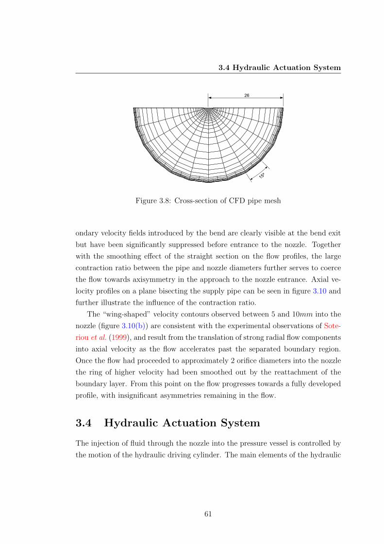
3.4 Hydraulic Actuation System
15º
26
Figure 3.8: Cross-section of CFD pipe mesh
ondary velocity fields introduced by the bend are clearly visible at the bend exit
but have been significantly suppressed before entrance to the nozzle. Together
with the smoothing effect of the straight section on the flow profiles, the large
contraction ratio between the pipe and nozzle diameters further serves to coerce
the flow towards axisymmetry in the approach to the nozzle entrance. Axial ve-
locity profiles on a plane bisecting the supply pipe can be seen in figure 3.10 and
further illustrate the influence of the contraction ratio.
The “wing-shaped” velocity contours observed between 5 and 10mm into the
nozzle (figure 3.10(b)) are consistent with the experimental observations of Sote-
riou et al. (1999), and result from the translation of strong radial flow components
into axial velocity as the flow accelerates past the separated boundary region.
Once the flow had proceeded to approximately 2 orifice diameters into the nozzle
the ring of higher velocity had been smoothed out by the reattachment of the
boundary layer. From this point on the flow progresses towards a fully developed
profile, with insignificant asymmetries remaining in the flow.
3.4 Hydraulic Actuation System
The injection of fluid through the nozzle into the pressure vessel is controlled by
the motion of the hydraulic driving cylinder. The main elements of the hydraulic
61

3.4 Hydraulic Actuation System
0.36 0.39
0.42
0.45
0.48
0.510.54
0.33
(a) plane across the bend exit
0.30.40.45
0.5
0.55
0.6
0.65
0.7
(b) plane 20mm before the nozzle entrance
Figure 3.9: Pipe half-sections showing isocontours of velocity magnitude (m/s).
Secondary velocity contours clearly evident at the bend exit, (a), are greatly
diminished before the flow enters the nozzle,(b).
62

3.4 Hydraulic Actuation System
r/Dp
V [m
/s]
-0.5 -0.25 0 0.25 0.5
0
0.2
0.4
0.6
0.8
1
15mm before nozzle20mm before nozzle25mm before nozzle30mm before nozzle40mm before nozzle50mm before nozzle
(a)
r/Dn
V [m
/s]
-0.5 -0.25 0 0.25 0.5
0
5
10
15
20
25
30
5mm into nozzle10mm into nozzle20mm into nozzle30mm into nozzle40mm into nozzle
(b)
Figure 3.10: Axial velocity profiles at various stream-wise distances (a) before
entrance to the nozzle and, (b) into the nozzle from the entrance plane.
63

3.4 Hydraulic Actuation System
driving system are: 4” diameter test fluid cylinder, 2 1/2” diameter double-
acting hydraulic cylinder, proportional control valve, fixed displacement vane
pump (31.8ml/rev), 15kW Electric motor and a 160L oil reservoir. The area
reduction ratio between the test fluid and hydraulic cylinder produces a maximum
pressure in the test fluid of 6MPa and a maximum volume flow rate of 1.5L/s.
Operational fluid pressure was limited to 1.5MPa by the design pressure of the
acrylic nozzle and pressure vessel. A technical schematic of the hydraulic system
can be found in appendix D.
As discussed in Section 3.1, injection of fluid through the test section is con-
trolled by the motion of the test fluid cylinder. This cylinder is coupled to the
double-acting hydraulic cylinder via a linear alignment coupler and shaft. The
position of the proportional control valve on the driving cylinder, controlled via a
±10V analog voltage sent from a control unit, governs the direction and flow rate
of hydraulic oil into the cylinder from the pump and reservoir. A “dead-band”
of cylinder movement existed between approximately -2.5V and +3V . After this
dead-band the piston velocity became roughly parabolic with input; a ‘+’ voltage
moving the piston forward, a ‘−’ voltage retracting the piston.
A Linear Displacement Transducer (LDT) within the piston bore allows for
highly accurate measurement of the instantaneous position of the piston. The
displacement signal was then differentiated to give piston velocity for each injec-
tion. The steady flow of hydraulic fluid from the fixed displacement vane pump
produced highly stable and repeatable piston velocity and allowed precise control
of the mass-flow through the test section.
To reduce disturbances to the flow in the supply pipe a custom end cap was
designed for the test fluid cylinder (see appendix D). A smooth bell-mouth shaped
contraction was used to transition the flow from the cylinder internal diameter
(101.6mm) to that of the supply pipe (52mm). CFD simulations indicated com-
plete removal of fluid recirculation zones in the end cap region under worst case
flow conditions.
During the test fluid cylinder filling process, described briefly in section 3.1,
suction pressure created by the retracting piston was used to drawn fluid into
the cylinder via a check valve and y-type strainer. Pressure drop data provided
by the check-valve manufacturer suggested a flow rate of less than 10L/min was
64

3.5 Optical Access Pressure Vessel
required to ensure that the liquid pressure remained above the vapour pressure
(suppression of cavitation). However, experience showed a retraction velocity
corresponding to <1L/min was required to prevent cavitation damage of the
spring-loaded ball within the check valve.
3.5 Optical Access Pressure Vessel
The optical access pressure vessel formed a critical part of the test facility and was
designed and fabricated for this study. As well as providing a means to control
the gas pressure downstream from the nozzle, and hence the cavitation within the
nozzle, viewing windows in the wall of the pressure vessel provided direct visual
access to the spray jet. This section provides an overview of the salient features
of the pressure vessel, however a complete list of engineering drawings can be
found in appendix C.
A schematic of the pressure vessel is shown in figure 3.11 and a list of the major
design parameters can be found in table 3.6. Nitrogen gas was supplied to the
vessel via a pressure regulator and supply valve, which provided coarse adjustment
of the gas pressure. Fine adjustment was then achieved by bleeding gas from the
vessel using a needle valve on a drainage line, allowing repeatability of gas pressure
conditions to within approximately ±3kPa. The volume of the pressure vessel
is such that the gas pressure increase due to the isothermal compression of the
quiescent gas during the period of liquid injection is kept to less than 2.6%. A
relief valve in the top of the vessel ensured gas pressures did not exceed 1.5MPa.
The pressure vessel featured nine viewing windows arranged in three axially
spaced sets of three orthogonal windows, referred to here as triplets. The loca-
tion and size of the viewing windows was strictly controlled by the design code,
AS1210-1997. The first triplet was positioned as close as possible to the base of
the vessel, with a centre distance of 142.4mm from the face of the bottom flange.
Each triplet was orientated 45 offset from the adjacent triplet to minimise the
axial spacing, with centre-to-centre distances of 177mm and 215mm between the
first and second, and second and third, triplets respectively. Heavy limitations on
the size of holes allowed in the torispherical dished ends of the vessel restricted the
65

3.5 Optical Access Pressure Vessel
1220
406
0
90
180
270
45
135225
315
596
596
180
270
0
90
ELEVATIONVIEW FROM 270 ORIENTATION
ORIENTATION PLANVIEW FROM TOP OF VESSEL
ELEVATIONVIEW FROM 0 ORIENTATION
ORIENTATION PLANVIEW FROM BASE OF VESSEL
= Ra 3.2 - Ra 6.3 um ALL OVER = ITEM NUMBER
= DETAIL NUMBER
1. SYMBOLS :-
FP
NOTES
= MEDIUM MACHINE, Ra 3.2 - Ra 6.3 um
= FULL PENETRATION
2. WELDS :-DETAIL DRAWINGS OF WELD TYPES CAN BE FOUND ON DRAWING SHEET 10.
3. NOZZLE NECK TO SHELL WELD - SEAL WELD GRIND FLUSH
DESIGN DATADesign Pressure 1.5 MPa
Design Temperature 65 C to -5 CHydro. Test Pressure 2.26MPa
Corrosion Allowance 0 mmP.W.H.T nll
Radiography nllHazard Level C
D
E
F
C
1 2 3 4
B
A
321 5
C
D
4 6 7 8
A
B
01
Cameron Stanley
WEIGHT:
A3
SHEET 1 OF 1SCALE:1:20
DWG NO.
TITLE:
REVISION: 7DO NOT SCALE DRAWING
DATE:
CONTACT
DEBUR AND BREAK SHARP EDGES
APPV'D
Ph:
DRAWN
UNSW
PRESSURE VESSEL
13/08/09
UNLESS OTHERWISE SPECIFIED:
DIMENSIONS ARE IN MMSURFACE FINISH:
TOLERANCES: 0.5 (02) 9385 6005
Figure 3.11: Pressure vessel - dimensions shown in mm.
66

3.5 Optical Access Pressure Vessel
Table 3.6: Pressure vessel design parameters
Property Value
Design Code AS1210-1997
Design Pressure (kPag) 1500
Test Pressure (kPag) 2260
Design Temperature (C) 50
Code Class 28
Hazard Level (AS4343) C
Material ASTM A240-304
Empty Weight (kg) 317
Volume (L) 123
Internal Diameter (mm) 388
Viewing port diameter (mm) 77.9 (bottom 3)
102.3 (top 6)
diameter of the lowest triplet ports to 77.9mm, whereas the diameter for the sec-
ond and third triplet was 102.3mm. The orthogonal layout of each triplet meant
back-lit photography, laser light-sheet illumination and Schlieren measurements
of the spray structure are possible at each axial location.
The design of the pressure vessel accommodated two major experimental con-
figurations (see figure 3.12);
• visualization and measurement of the cavitation in the nozzle with the test
section held outside the pressure vessel, and,
• interrogation of the near nozzle spray structures with the test section in-
serted into the base of the pressure vessel.
The test section is fixed in position between a flange on the upper end of
the supply pipe and the bottom of the pressure vessel. When nozzle cavitation
structure and turbulence is to be measured a removable adapter flange (item 4)
is fixed to the base of the pressure vessel. A 10mm extension of the test piece
67

3.5 Optical Access Pressure Vessel
B
B
C
SECTION B-B SCALE 1 : 10
DETAIL C SCALE 1 : 5
1
2
3
411
3
6
5
12
3
7
8
9
8
10
D
E
F
C
1 2 3 4
B
A
321 5
C
D
4 6 7 8
A
B
01
Cameron Stanley
WEIGHT:
A3
SHEET 1 OF 1SCALE:1:50
DWG NO.
TITLE:
REVISION: 2DO NOT SCALE DRAWING
DATE:
CONTACT
DEBUR AND BREAK SHARP EDGES
APPV'D
Ph:
DRAWN
UNSW
PRESSURE VESSEL
22/05/09
UNLESS OTHERWISE SPECIFIED:
DIMENSIONS ARE IN MMSURFACE FINISH:
TOLERANCES: 0.5 (02) 9385 6005
(a) Test section configuration for nozzle cavitation interrogation.
C
C
SPRAY CONFIG
SECTION C-C SCALE 1 : 10
11
3 5
D
E
F
C
1 2 3 4
B
A
321 5
C
D
4 6 7 8
A
B
01
Cameron Stanley
WEIGHT:
A3
SHEET 1 OF 1SCALE:1:50
DWG NO.
TITLE:
REVISION: 2DO NOT SCALE DRAWING
DATE:
CONTACT
DEBUR AND BREAK SHARP EDGES
APPV'D
Ph:
DRAWN
UNSW
PRESSURE VESSEL
22/05/09
UNLESS OTHERWISE SPECIFIED:
DIMENSIONS ARE IN MMSURFACE FINISH: 63
TOLERANCES: 0.5 (02) 9385 6005
(b) Test section configuration for near-nozzle spray interrogation.
Figure 3.12: Pressure vessel section view. Configuration (a) allows optical
access to the test section for cavitation interrogation; Configuration (b) allows
optical access to the exit plane of the nozzle for spray structure investigation.
Note: all bolts and piping connections are suppressed for clarity.
68

3.6 Support Frame
Table 3.7: Pressure vessel assembly component list (figure 3.12)
Item # Description
1 Pressure vessel drainage port
2 Pressure vessel base flange
3 O-ring
4 Removable adapter flange
5 Supply pipe flange
6 Pressure sensor and thermocouple port
7 Pressure vessel viewing port flange
8 Gasket
9 Glass window
10 Window retaining ring
11 Acrylic nozzle test section
12 Supply pipe drainage port
beyond the exit plane of the orifice allows the tip of the test section to be inserted
into a recess in the adapter flange, holding the nozzle outside of the vessel with
the orifice entirely visible (see figure 3.12(a)).
For viewing and measurement of the near nozzle spray structure the locating
flange is removed and the acrylic nozzle inserted into the base of the pressure
vessel. In this configuration, the exit plane of the nozzle is vertically aligned with
the lowest viewing window (figure 3.12(b)). Test fluid that accumulates in the
base of the PV when the nozzle is in this configuration can be drained from the
base of the PV through a drainage port (item 1) in the torispherical head, and
returned to a settling tank.
3.6 Support Frame
The general frame structure was designed to support the major components of
the rig, allow optical access to the acrylic nozzle for visualisation and diagnostics
69

3.7 Test Liquid Characterisation -Sodium Iodide
and support measurement instrumentation. The major frame structure was bro-
ken into two components; the support frame for the pressure vessel and supply
piping, and the support frame for the hydraulic and test fluid cylinders. Supple-
mentary to these is an independent spacing structure between the two hydraulic
cylinders. This ensured the large forces generated by the hydraulic cylinder were
held independently of the light-weight cylinder support structure. Leveling feet
under the base of both frame structures allows the test piece to be leveled.
To accommodate the two flow interrogation configurations discussed in Section
3.5 the pressure vessel is moved vertically relative to the test section. Lifting of
the pressure vessel was performed using a block and tackle mounted to an I-
beam at the top of the support frame and attached to lifting lugs on the top of
the PV. Mounting brackets supporting the PV allow it to be bolted in various
set positions.
Positioning of the high speed camera was controlled using a three-axis linear
positioning stage attached to an aluminium plate mounted to the support frame
roughly level with the base of the acrylic nozzle. An adapter plate was then used
to attach the camera to the positioning stage at the correct working distance.
This method ensured the camera was positioned at 90 to the flat faces on the
acrylic nozzle and allowed accurate adjustments of lens focus or camera position.
3.7 Test Liquid Characterisation -
Sodium Iodide
3.7.1 Refractive Index Matching
To prevent optical distortion during visualisation, refractive index matching be-
tween the acrylic nozzle and the test fluid was employed. A number of liquids exist
which allow refractive index matching with acrylic (n ≈ 1.49), each have their
individual merits and shortcomings. Consideration must be given to chemical
reactivity, harmfulness to the operator, solution viscosity and price. A tabulated
list of solids and potential matching fluids can be found in Budwig (1994) and
Miller et al. (2006). For this study aqueous sodium iodide solution was selected
as the test fluid.
70

3.7 Test Liquid Characterisation -Sodium Iodide
Sodium iodide has been used in a number of studies to achieve refractive
index matching. Chen & Fan (1992) and Reese et al. (1995) used a 55% w/w
aqueous solution of NaI in a rectangular glass chamber enclosing their cylindri-
cal Pyrex glass test section (n ≈ 1.47) to improve optical access and minimise
curvature effects during Particle Image Velocimetry (PIV) measurements. Uzol
et al. (2002) employed a 64% w/w NaI solution as their test fluid to conduct
PIV measurements in an axial turbo-pump constructed from acrylic (PMMA).
In this article, the authors discuss some of the difficulties associated with us-
ing NaI mixtures, including chemical stability and variations in transmittance.
Sodium iodide solutions are susceptible to discolouration due to the formation
of I3− ions, a process accelerated by exposure to light, oxygen and elevations in
temperature. Unlike I− ions, I3− ions absorb light in the visible range, which can
dramatically attentuate the passage of light and affect visualisation. This process
can be minimised by limiting the solutions exposure to light and oxygen, the later
of which is achieved by keeping the solution under the presence of Nitrogen gas.
It has also been shown that I3− ions can be partially elliminated from the solution
by the addition of either sodium borate 10-hydrate (Na2B4O7.10H2O) (see Uzol
et al. (2002)) or sodium thiosulphate (Na2S2O3) (see Narrow et al. (2000)) at a
concentration of 0.1% w/w. For the current work sodium thiosulphate has been
used as the I3− ion mitigating agent.
A simple model for the prediction of refractive index, nNaI , of NaI solutions
as a function of temperature T, NaI concentration C, and wavelength λ was
determined by Narrow et al. (2000) for moderate parameter variations:
nNaI (T,C, λ) = 1.252−(2.91× 10⁻⁴C−1
)T +
(0.365)C + (5542nm2)λ−2 (3.7)
Equation 3.7 provides a very good estimate of the solution concentration re-
quired to achieve refractive index matching with acrylic for a given liquid tem-
perature and light wavelength, although it must be noted the range of conditions
used within this work exceeds those used to form the correlation. In practice, it
is common to obtain the solution concentration using a trial and error process,
71

3.7 Test Liquid Characterisation -Sodium Iodide
visually comparing the distortion of light passing through the mixture (see Lim
et al. (1994) and Miller et al. (2006)).
For this work comparisons were made of the optical distortion of a uniform
1mm × 1mm grid placed behind the test section as solution concentration was
varied from 57% to 64% (w/w) in 1% increments. Photos of the mesh were taken
for each concentration as the liquid temperature was slowly increased from 13 C
to approximately 20 C. The coefficients of equation 3.7 indicate that changes in
concentration have a greater influence on refractive index than changes in tem-
perature. This agreed well with experimental observations. As such, a nominal
concentration of C = 63% was selected for use in all tests as it exhibited the
least distortion of the grid pattern at the temperature expected for experimental
measurements (T ≈ 18 C). Despite this, no active temperature control was used.
Figure 3.13 shows the effectiveness of the refractive index matching technique.
(a) (b)
Figure 3.13: Experimental refractive index matching showing the distorion of a
1× 1mm2 mesh placed behind the test section. The nozzle diameter is clearly
present for (a) distilled water (control) but is near invisible for (b) 63%w/w NaI
solution.
72

3.7 Test Liquid Characterisation -Sodium Iodide
3.7.2 Kinematic Viscosity
Data for viscosity and density of NaI solutions was rather limited in the litera-
ture. Some studies used the nominal values of 1.8 and 1.1×10⁻⁶ m2/s for specific
gravity and kinematic viscosity respectively (see Uzol et al. (2002)). Given the
inevitable variations to these parameters with temperature and concentration,
viscosity measurements were conducted using a Cannon-Fenske Routine viscome-
ter for a range of NaI concentrations from 57% to 66% for temperatures between
13 C and 24 C. Measurements at each temperature were repeated twice to min-
imise measurement error. A multi-variable regression equation was then used to
generate an expression for relate kinematic viscosity in terms of temperature and
concentration. The resulting regression equation is:
ν = 8.575× 10⁻⁶e(−0.014T )C3 (3.8)
where T is the liquid temperature in C and C is solution concentration in %w/w.
A comparison of the measured viscosity to that predicted by equation 3.8 is shown
in figure 3.14.
= 8.575x10⁻⁶e-0.014TC3
meas [ 10-6 m2/s]
pre
d [ 1
0-6 m
2 /s]
1 1.2 1.4 1.6 1.8 2 2.21
1.2
1.4
1.6
1.8
2
2.2
Figure 3.14: NaI kinematic viscosity regression
73

3.7 Test Liquid Characterisation -Sodium Iodide
3.7.3 Density
Density measurements were also conducted for the same range of NaI concen-
trations at laboratory temperature (T ≈ 18 C). A nominal volume (20mL) of
liquid was accurately transferred to a beaker using a high resolution pipette. This
volume was then weighed and the density calculated. The process was repeated
5 times for each concentration to improve accuracy. The expected uncertainty
in the density of the sodium iodide solution with temperature change was es-
timated using the percentage variation in density of saturated water across the
expected experimental temperature variation. A plot of density variation with
concentration can be seen in figure 3.15 together with a linear regression equation.
= 22.61C + 442.36
C [% w/w]
[k
g/m
3 ]
56 58 60 62 64 661700
1750
1800
1850
1900
1950
Figure 3.15: NaI density as a function of solution concentration
74

3.8 Data Acquisition and Cylinder Control
3.7.4 Vapour Pressure
Vapour pressure for the NaI solution was determined using an empirical formu-
lation based on the Antoine type equation:
log [Pv (kPa)] = A (m) +B (m)
T (K)+
C (m)
T (K)2 (3.9)
where A(m), B(m) and C(m) are cubic functions of solution molarity. The con-
stants for each of these equations were (Patil et al. (1991)): A0 = 6.642, A1 =
0.491, A2 = −0.101, A3 = 0.005, B0 = −1340.491, B1 = −323.215, B2 = 63.051, B3 =
−3.272, C0 = −146462.900, C1 = 51849.160, C2 = −10123.010, C3 = 525.534.
Figure 3.16 shows a plot of vapour pressure variation with temperature.
T [°C]
Pv [
kPa]
0 5 10 15 20 25 30
0.6
0.8
1.0
1.2
1.4
Figure 3.16: NaI vapour pressure as a function of temperature
A summary of the typical properties for a 63%w/w NaI solution at a nominal
temperature of T = 18 C are listed in table 3.8.
3.8 Data Acquisition and Cylinder Control
A number of parameters were recorded during each injection using a National In-
struments PCI6221 multifunction data acquisition (DAQ) card. The DAQ card
75

3.8 Data Acquisition and Cylinder Control
Table 3.8: Physical Properties of Aqueous Sodium Iodide
Property Nominal Value
Concentration, C %(w/w) 63
Refractive Index, n 1.49
Kinematic Viscosity, ν (m2/s) 1.67 ×10⁻⁶
Density, ρ (kg/m3) 1866.79
Vapour Pressure, Pv (kPa) 0.97
was 16-bit resolution and with 16 analog input and 2 analog output channels,
with a combined sample rate of 250kHz. The DAQ card was interfaced with a
standard PC using National Instruments LabVIEW 2009 program. A state ma-
chine style control program was written which allowed for various programmable
piston motion sequences, such as that used to fill the test fluid cylinder with fresh
NaI following an injection cycle. During the expulsion phase of the injection se-
quence, data was acquired and saved for injection pressure, P1, gas pressure,
P2 and piston position. Sample rates were limited to the response time of the
pressure sensors and set to 1000Hz for all variables. Data acquired from each
injection was later processed using Matlab, described in chapter 4.
As well as acquiring measurement data, the program used digital input/output
from the DAQ card to operate a number of relays within the system including
that used to control the pneumatically actuated ball valve and activation of the
hydraulic control unit. Digital output synchronised to the position of the piston
were also used to trigger the acquisition of high-speed video recordings. Piston
velocity was controlled for each injection by selecting the analog voltage to be
output to the hydraulic control unit.
Temperature measurements for the liquid, gas and ambient air were continu-
ally acquired using a Pico USB TC-08 Thermocouple Data Logger. Samples were
acquired at 1 minute intervals over the duration of experiments each day. Later,
the temperature used to evaluate the liquid properties for a particular injection
was determined by correlating the time-stamps on the DAQ measurements.
76

Chapter 4
Measurement Techniques and
Experimental Uncertainty
This chapter provides the details of the experimental techniques and methodolo-
gies used throughout this work. In order to process the high speed visualisation
a number of image processing programs were written and used to determine the
results presented in chapter 5. The mathematical formulations and techniques
for determining flow features central to these programs will be discussed. Finally
estimates of the sources of error and measurement uncertainty will be provided.
4.1 Data Extraction
Measurements of injection pressure, gas pressure and piston position were recorded
during each injection at a sample rate of 1000Hz by the data acquisition system
described in section 3.8. Injection pressure traces typically showed transient
spikes associated with the initial motion of the piston and the end of injection.
These sections of the data were removed before processing, to ensure all derived
parameters were determined from steady state data only.
In many cases injections were composed of a number of distinctly different
operating phases. These corresponded to the formation of different cavitation
structures within the orifice and produced significant changes in the injection
pressure. These changes in pressure are a consequence of the shifts in the dis-
charge coefficient that result from the various degrees of cavitation. As the system
77

4.1 Data Extraction
was driven by a constant mass flow (constant piston velocity), variations to the
discharge coefficient cause the shifts in the injection pressure to satisfy mass con-
tinuity. Where possible, data for each of these discrete regions in the record was
separated and processed individually. Figure 4.1 shows typical pressure traces in-
dicating multiple steady state sections and the removal of transients in the data
record of an injection.
A Matlab program was used to conduct all calculations from the steady state
data. Injection and gas pressures are averaged over the steady state region before
being used to calculate the non-dimensional parameters; cavitation number and
nozzle discharge coefficient. Piston velocity was determined from the gradient of
a linear regression of piston position data for the recorded interval. The mean
nozzle velocity was then determined using continuity and the ratio of cylinder to
nozzle diameters.
Temperature measurements of the pressure vessel gas, liquid in the supply
pipe and ambient air were measured at 1 minute intervals for the duration of
experiments each day using k-type thermocouples. The temperature used for the
determination of fluid properties such as viscosity (section 3.7) was taken as the
mean of the liquid temperature for the two data points either side of the actual
injection time.
4.1.1 Non-dimensional Parameters
Data averaged over the steady state sections of the data record were used to
calculate the non-dimensional parameters of interest; Reynold number, Re, cav-
itation number, K and discharge coefficient, Cd. Reynolds number was defined
here as,
Re =VnDn
ν(4.1)
where Vn is the mean velocity through the nozzle, Dn is the nozzle diameter and
ν is the kinematic viscosity.
As mentioned in section 1.3.4 the cavitation number used in this work is
defined as,
78

4.1 Data Extraction
P1 - INJ. PRESSURE
P2 - GAS PRESSURE
t [s]
P [k
Pa]
0 1 2 3 40
50
100
150
200
250
300
350
400
(a)
P1 - INJ. PRESSURE
P2 - GAS PRESSURE
t [s]
P [k
Pa]
0 0.5 1 1.5 2 2.5 3 3.50
200
400
600
800
(b)
Figure 4.1: (a) Single flow regime pressure trace for Re = 6.62× 10⁴ and
K = 1.84. (b) Multiple flow regime pressure trace for Re = 8.0× 10⁴ with
K = 1.35 initially and K = 1.58 late. Grey regions in the plot indicate transient
data rejected in analysis.
79

4.1 Data Extraction
K =P1 − PvP1 − P2
. (4.2)
where P1 is the injection pressure, P2 is the gas pressure, and Pv is the vapour
pressure. Both P1 and P2 were measured using Honeywell piezoresistive pressure
transducers (gage) with a response time < 1ms. The pressure sensor for P1 was
mounted in a tapping in the supply pipe 202mm (item 6 in figure 3.12) below
the nozzle entrance. Similarly, the pressure sensor for P2 was mounted on a side
branch of the filling port on the top of the pressure vessel (visible in figure 3.11).
P1 was converted to absolute pressure for use in equation 4.2 by the addition
of atmospheric pressure, measured using a barometer in the laboratory, prior to
commencement of experiments each day.
The discharge coefficient of a nozzle relates the actual mass flow rate through
the nozzle, mact, to the theoretical mass flow rate, mth for an ideal fluid under
identical conditions,
Cd =mact
mth
. (4.3)
The theoretical mass flow rate can be expressed in terms of the Bernoulli velocity
through the nozzle, Vnth, the nozzle cross sectional area, A, and the liquid density,
ρ,
Cd =mact
ρAVnth
. (4.4)
The actual mass flow rate through the nozzle can be expressed in terms of the
piston velocity, Vc, and test fluid cylinder diameter, Dc. An expression for the
theoretical velocity through the nozzle can be obtained by combining Bernoulli’s
equation and mass continuity between points upstream of the entrance and nozzle
exit. Substitution of these expressions into equation 4.4 yields
Cd =D2cVc
D2n√
1−β4
√2(P ∗
1−P ∗2 )
ρ
(4.5)
80

4.2 High-speed Visualisation
where P ∗i = Pi + ρgzi, denotes piezometric pressure at point i, Dn is the nozzle
diameter, and β = Dn/Dp is ratio of the nozzle to supply pipe diameters.
Discharge coefficient is often expressed as the product of two different pa-
rameters: the velocity coefficient, Cv, and the area contraction or contraction
coefficient, Cc. The velocity coefficient accounts for the reduction from ideal ve-
locity, and the contraction coefficient accounts for the loss of cross-sectional area
due to flow contraction. In this way the the discharge coefficient can be expressed
as
Cd = CvCc (4.6)
The expression in equation 4.6 is helpful for analysing the elemental sources of
loss and will be called upon in the discussion of chapter 5.
4.2 High-speed Visualisation
High-speed visualisation provided a non-intrusive means of exploring the temporal
evolution of the cavitation structures within the nozzle and the near nozzle spray
structure. A Phantom V7.3 CMOS camera (800 x 600 pixel) was used for all high-
speed visualisation in this work. This camera has a full resolution frame rate of
6688 frames per second (fps), with frame rates in excess of 100kfps capable at
reduced resolution. These capabilities allowed for visualisation at high resolution
on temporal scales that provided great insight into the cavitation initiation and
development, bubble shedding process and spray ligament formation. Acquisition
of the images was initiated by a trigger pulse synchronised to the piston position.
The axial position of the piston chosen as the trigger point for the camera was
dependent on the piston velocity and desired frame rate of the camera.
4.2.1 Illumination
The appropriate choice and application of light to the test piece is arguably the
most important and complex element of scientific photography (Blaker (1965)).
81
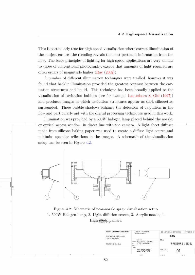
4.2 High-speed Visualisation
This is particularly true for high-speed visualisation where correct illumination of
the subject ensures the recoding reveals the most pertinent information from the
flow. The basic principles of lighting for high-speed applications are very similar
to those of conventional photography, except that amounts of light required are
often orders of magnitude higher (Ray (2002)).
A number of different illumination techniques were trialled, however it was
found that backlit illumination provided the greatest contrast between the cav-
itation structures and liquid. This technique has been broadly applied to the
visualisation of cavitation bubbles (see for example Lauterborn & Ohl (1997))
and produces images in which cavitation structures appear as dark silhouettes
surrounded. These bubble shadows enhance the detection of cavitation in the
flow and particularly aid with the digital processing techniques used in this work.
Illumination was provided by a 500W halogen lamp placed behind the nozzle,
or optical access window, in direct line with the camera. A light sheet diffuser
made from silicone baking paper was used to create a diffuse light source and
minimise specular reflections in the images. A schematic of the visualisation
setup can be seen in Figure 4.2.F
F
H
SECTION F-F SCALE 1 : 10
DETAIL H SCALE 1 : 5
1 42 3D
E
F
C
1 2 3 4
B
A
321 5
C
D
4 6 7 8
A
B
01
Cameron Stanley
WEIGHT:
A3
SHEET 1 OF 1SCALE:1:50
DWG NO.
TITLE:
REVISION: 2DO NOT SCALE DRAWING
DATE:
CONTACT
DEBUR AND BREAK SHARP EDGES
APPV'D
Ph:
DRAWN
UNSW
PRESSURE VESSEL
22/05/09
UNLESS OTHERWISE SPECIFIED:
DIMENSIONS ARE IN MMSURFACE FINISH: 63
TOLERANCES: 0.5 (02) 9385 6005
Figure 4.2: Schematic of near-nozzle spray visualisation setup
1. 500W Halogen lamp, 2. Light diffusion screen, 3. Acrylic nozzle, 4.
High-speed camera
82

4.3 Image Processing Techniques
4.2.2 Camera Lens and Region of Interest
Careful selection of the camera region of interest (ROI) was important to ensure
the trade off between frame rate and spatial resolution was optimised for the
flow structures being recorded. Fundamental to this optimisation was the correct
choice of camera lens. For internal nozzle flow analysis a 105mm Nikon Nikkor lens
was used at a typical f-number of 11, providing maximum spatial resolution along
the stream wise direction. With this lens the 800 pixel width of the camera CMOS
chip was mapped as close as possible to the 40mm length of the nozzle, providing
a spatial resolution of ≈ 0.055mm/pix. In the lateral direction the camera region
of interest (ROI) was reduced to just cover the width of the nozzle. This resulted
in a ROI of 800 pixels x 160 pixels with a maximum frame rate capability of
23121fps. For near nozzle spray analysis a 70-200mm Carl Zeiss Jena f/2.8-4
MC Macro lens was used at a typical f-number of 8. A camera resolution of 608
x 400 pixels provided a suitable compromise between field of view and camera
frame rate, allowing 12121fps with a spatial resolution of ≈ 0.092mm/pix. A
schematic illustrating the ROI for both configurations can be seen in figure 4.3.
In order to reduce the working distance of the camera using these high focal
length lenses, lens spacers (extension tubes) were placed between the camera and
the lens, artificially increasing the image distance. This allowed the camera to
be mounted to a 3-axis translation stage attached to the rig frame, which aided
with focusing and positioning the ROI with respect to the test section.
4.3 Image Processing Techniques
Once recordings were taken of the cavitation the extraction of pertinent flow
details required digital processing of the images sequences. All recordings pre-
sented in this work represent recordings under steady flow conditions. Images
recorded using the Phantom V7.3 camera were converted to 8-bit multitiff image
sequences, a format suitable for processing using Matlab. A number of programs
were written in Matlab for the extraction of different information from the video
recordings such as; cavitation collapse length, shedding frequency, and spray an-
83
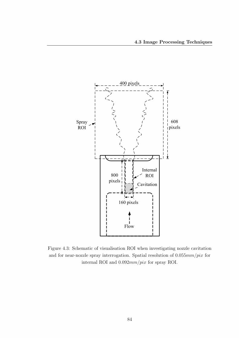
4.3 Image Processing Techniques
Internal ROI
Flow
Spray ROI
160 pixels
Cavitation
800 pixels
608pixels
400 pixels
Figure 4.3: Schematic of visualisation ROI when investigating nozzle cavitation
and for near-nozzle spray interrogation. Spatial resolution of 0.055mm/pix for
internal ROI and 0.092mm/pix for spray ROI.
84

4.3 Image Processing Techniques
gles. The major interrogation methods employed during image processing for
each of these measurements will be described in detail in the following sections.
4.3.1 Cavity Collapse length
The measurement of cavity collapse length is common for cavitation experiments
for both internal and external flows. Often this measurement is via the analysis
of photographs or video recordings. However, little attention is afforded to out-
lining the method used to identify a single collapse length for what is invariantly
a 3-dimensional flow structure. For example, Sou et al. (2010) reports measure-
ments of collapse length in 4mm diameter plain orifice nozzles as “the mean value
obtained using 10 photographs for each flow rate”. Using a camera frame rate
of 20, 000fps, it is likely that this number of image frames would be insufficient
to capture one full period of the cavitation shedding which could be expected for
some of their flow conditions.
The highly transient nature of the bubble collapse process can result in sig-
nificant frame-frame variation in observed cavity length. For the current work
attempts were made to determine a collapse length that represented a spatially
and temporally averaged value for each recording. The cavity length has been
defined here as the distance from the nozzle entrance to the last point in the
stream-wise direction at which the location of cavitation or bubbles can be iden-
tified.
To aid with the detection of cavities and bubbles the original recordings of
the cavitation, typically 4500 frames in length, were converted to binary (white
representing liquid phase, black representing vapour) by the application of a suit-
able greyscale threshold. This threshold was adjusted for each recording to ensure
that fine bubble clouds that were still considered part of the cavitation structure
were not eliminated during the conversion process. The Matlab program would
then extract profiles of pixel value along 20 vertical lines extending the length of
the nozzle, which were evenly spaced between the left and right walls. The up-
permost interface between the vapour and liquid region was then identified as the
last stream-wise pixel to have zero greyscale value (representing the edge of the
black cavitation region). The temporal evolution of the cavity interface for each
85

4.3 Image Processing Techniques
of the 20 lateral positions was then averaged, both in time and space, to produce
a nominal value for the mean cavity collapse length. The maximum, minimum
and standard deviation of the cavity collapse length were also determined. A
typical frame from an unprocessed image sequence and the corresponding binary
frame can be seen in figure 4.4(a) and figure 4.4(b) respectively. Figure 4.4(c)
shows the statistical collapse length measurements projected over the top of the
original unprocessed frame from figure 4.4(a).
(a) (b)
maximummean + st. dev.meanmean - st. dev.minimum
Nozzle Entrance
(c)
Figure 4.4: Collapse length image processing: (a) a typical frame for
Re = 9.3× 10⁴ and K = 2.01 before conversion, (b) the same frame represented
as a binary image and (c) statistical collapse length over-layed on original
frame. Note: a reduced length of nozzle shown only.
For developed cavitation, cavities tend to collapse very near the exit of the
nozzle and it is common to observe clouds of cavitation bubbles being convected
through the exit plane. The precise collapse length under these conditions cannot
be determined accurately. The number of times the cavity was identified as
reaching the nozzle exit was counted for each recording and gave an indication for
the extent to which the true collapse length had been “clipped” by this limitation.
Cases of supercavitation and hydraulic flip could not be processed as the cavities
86

4.3 Image Processing Techniques
are all exceeding the nozzle length. These cases were assigned a normalised
collapse length of 1.
Refraction of the light passing through the nozzle for the cases with water as
the working fluid significantly affected the contrast between the cavitation and
the fluid. The conversion to binary was impossible whilst maintaining a true
representation of the cavitation structure. To avoid this problem only the central
core of the image (≈ 1/3 width), where cavitation could be easily distinguished
from liquid, was used for estimation of the collapse length using an otherwise
identical method to that described above. However, as the measurement was
obtained for a smaller region of the flow, the estimate of collapse length is not as
robust as for sodium iodide.
4.3.2 Spray Angle
Similarly to collapse length, spray angle is a parameter widely reported in the
literature, but is often loosely defined. For small scale nozzles the spray angle
is often estimated by the angle formed between tangent lines passing through
the nozzle tip along the edge of the spray surface in the “steady” region (see for
example Desantes et al. (2006)). This region describes the conical section of the
spray immediately after the exit of the nozzle, the length of which varies based
on injection conditions. Payri et al. (2004) estimate its length to equal 60% of
the jet penetration and use this length of spray to estimate spray angle. Break-
up lengths for large-scale nozzles are significantly greater than those for small
nozzles. This makes visualising the entirity of the spray very difficult and means
estimates of spray angles are generally made using the near-nozzle region of the
jet.
For the current work the focus of the spray visualisations was on investigat-
ing the influence of the cavitation within the nozzle on the influence on the spray
structures in the region immediately after the nozzle exit. As such, attempts were
made to minimise the error in the estimate of spray angle taken from spray record-
ings encompassing a relatively short length of jet (≈ 6Dn). Video recordings were
digitally averaged over the 4500 frame record length before being converted to
binary by the application of a greyscale threshold. As for the determination of
87

4.3 Image Processing Techniques
collapse length, the threshold used for conversion to binary was manually chosen
for each recording to suit the relative greyscale intensity of each averaged image.
Repeated trials on the same injection image indicated the spray angle was insen-
sitive to variations in this parameter within sensible limits (discussed in section
4.3.4). Figure 4.5 shows a representational spray image, the digitally averaged
frame and the corresponding binary frame for the given conditions.
(a) (b) (c)
Figure 4.5: Spray images for Re = 6.5× 10⁴ and K = 1.83 showing (a) Single
frame from image sequence, (b) Average spray image, (c) Average spray
converted to binary image.
Once converted to binary the upper and lower vertical limits for the measure-
ment of the angle, denoted yUL and yLL respectively, were selected. These points
formed the bounds for a series of 10 pairs of equally spaced horizontal lines pass-
ing through the spray image. A schematic representation of the spray indicating
the half angles and relevant geometric points can be seen in figure 4.6.
The lateral locations of the gas/liquid interface for the ith pair of horizontal
intersecting line are denoted as xLU(i) and xRU(i) for the left and right upper
points respectively, and xLL(i) and xRL(i) for the left and right lower points
respectively. These values are obtained by determining the distance along the
88

4.3 Image Processing Techniques
Spray
Nozzle
Flow
Upper Limit = yUL
Lower Limit = yLL
yL(i)
yU(i)
xRL(i)
xRU(i)
vertical reference
y
x
θR(i)θL(i)
xLL(i)
xLU(i)
Figure 4.6: Spray angle definition - right side shown
horizontal transect from an arbitrary reference point to the first and last zero
value elements through the binary spray.
The vertical translation between each pair of lines was set to five pixels, how-
ever the spacing between the upper and lower line was unique to each spray and
set to provide maximum coverage of the spray without exceeding the bounds
identified. In this fashion the vertical coordinate of the upper spray edge for the
ith line pair, yU (i), can be written in terms of the distance from the upper limit
as,
yU (i) = yUL + 5 (i− 1) . (4.7)
Similarly the lower spray edge for the ith line pair, yL (i) can be expressed in
terms of the distance from the lower limit as,
yL (i) = yLL − 5 (10− i) . (4.8)
Estimates for the half angle on both the left, θL, and right, θR, edges of the
spray were then calculated as the mean angle determined between the upper and
89

4.3 Image Processing Techniques
lower gas/liquid interface for each of the 10 bisecting line pairs,
θR =1
10
10∑i=1
arctan
(xRU (i)− xRL (i)
yU (i)− yL (i)
)(4.9)
θL =1
10
10∑i=1
arctan
(xLL (i)− xLU (i)
yU (i)− yL (i)
)(4.10)
The overall estimate of the spray half angle could then be determined as,
θ =1
2(θL + θR) (4.11)
where averaging the half angle for the left and right sides of the spray eliminates
errors introduced by possible vertical misalignment of the nozzle with respect to
the axis of the camera. For highly divergent jets the reduction of image resolution
required to achieve suitable frame rates meant that one side of the spray structure
was analysed only. The measured half angle in these cases was corrected for nozzle
misalignment using the mean angle of a number of hydraulically flipped cases for
the same camera setup.
4.3.3 Signal Spectral Analysis
To determine the frequencies associated with the unsteady cloud shedding within
the nozzle a spectral analysis technique was applied to the video recordings. The
most common method of spectral analysis involves calculating the power spectral
density (PSD) of the recording. Before describing the specific way in which this
analysis was applied to the cavitation recordings, a brief technical description of
the spectral analysis is given. The mathematical formulations within are derived
mostly from Mirchandani (2011).
4.3.3.1 Power Spectral Density
In signal analysis the power spectral density provides a means of describing how
the average power of a signal is distributed with frequency. For a discrete-time
random process, x (n) for n = 0, . . . , N − 1, the PSD can be expressed as
90

4.3 Image Processing Techniques
SXX (ω) = limM→+∞
E 1
2M + 1|
M∑n=−M
x (n) e−jωn|2 (4.12)
where E is the expectation operator. It should be noted that the term “power”
is used in PSD analysis in the sense of a squared variable and can be related to
physical power in some cases by a dimensional scaling constant (Randall (1987)).
In simple terms equation 4.12 states that the power spectral density of a
random process that has been discretely sampled in time can be estimated by
taking the magnitude squared of the Discrete-time Fourier Transform (DTFT)
of the data x (n) and dividing by the length of the record. Then, since the
Fourier transform will be a random variable (each new x (n) will be different),
the expected value (i.e. average value) is taken. Finally, since the random process
is generally of infinite duration, the limit is taken.
The problem is that data records are always finite. One of the most common
methods used for estimating the PSD for a finite length data signal is known as
the Periodogram. Derived from equation 4.12, the summation is formed over a
finite data length and by removing the expectation operator, it is defined as
SPER (ω) =1
N|N−1∑n=0
x (n) e−jωn|2 (4.13)
which is the DTFT squared and averaged. However the variance of the peri-
odogram spectral estimator does not approach zero for N → ∞, which may be
due to the removal of the expectation operator, that is, a lack of averaging. To
improve the variance of the estimator, the expectation operator from equation
4.12 can be replaced by averaging a set of periodograms. If we assume there are
K independent records of the random process available for the interval 0 ≤ n < L
then we can define the averaged periodogram estimator as,
SAV PER (ω) =1
K
K−1∑m=0
S(m)PER (ω) (4.14)
where S(m)PER (ω) is the periodogram for the mth data set defined by,
S(m)PER (ω) =
1
L|L−1∑n=0
xm (n) e−jωn|2. (4.15)
91

4.3 Image Processing Techniques
In the case that each xm (n) for m = 0, 1, 2 . . . was a unique realisation of a
random process, then the DTFT would be unique and the averaging results in a
reduction of the variance of the PSD estimator by a factor of K. However more
commonly the estimate of the PSD must be made from a single data record of
length L. One means for reducing the variance of the PSD estimate from a single
record is known as Welch’s method (Welch (1967)). In this method an average is
determined for the periodograms of a number of overlapping segments from the
same data set offset by a separation D such that the kth sequence can be written,
xk (n) = x (n+ (k − 1)D) , n = 0, 1, . . . , L− 1.
Visually this segmentation of the single data record can be seen in figure 4.7
X(n)0 N – 1
0 L – 1
D D + L + 1
m – L N – 1
X1(n)
X2(n)
Xk(n)
Figure 4.7: Schematic of the signal segmentation using Welch’s averaged
periodogram
The Fourier Transform, or in this case the Discrete-time Fourier Transform
makes the implicit assumption that the signal is repetitive. In other words the
segment of the record within the measured time repeats for all time. In reality,
measured signals have discontinuities between the start and end of the record.
Without correction the DTFT assumes these discontinuities are part of the re-
peating signal, which introduces artificial broad frequency spectra. By multi-
plying the time signal by a window function, w(n), the record can be reduced
smoothly to zero at each end enforcing end-point continuity.
92

4.3 Image Processing Techniques
Welch’s averaged periodogram can be written in terms of the windowed data
record as follows,
SW (ω) =1
KLU
K−1∑k=0
|L−1∑n=0
w (n)xk (n) e−jωn|2 (4.16)
where U is a constant accounting for the effect of the window on the power
estimate, defined as
U =1
L
L−1∑n=0
|w (n) |2 (4.17)
The primary advantage of Welch’s method over other PSD methods is that by
overlapping the segments the average can be conducted over more periodograms,
improving the variance in the output.
4.3.3.2 Calculation Method
In order to evaluate the spectral properties of the cavity shedding the video
recording was first analysed to select an appropriate position in the collapse region
for the analysis. A stream-wise location was carefully selected that correspond to
a point in the collapse region through which the shed cloud regularly passed as it
was transported by the bulk flow, but was not a location permanently occupied by
the fixed cavity. In other words, the greyscale values at these locations contain the
temporal variations in intensity reflecting the large-scale cavity shedding process.
Once the stream-wise position was determined the images were then analysed
using a program written in Matlab. Unlike the analysis techniques described in
sections 4.3.1 and 4.3.2, the spectral analysis did not require conversion of the
image to binary. The greyscale signal for 10 pixels spaced evenly across the width
of the nozzle was then extracted from the image sequence. A schematic represen-
tation of the 10 chosen interrogation pixels is shown in figure 4.8. To eliminate
the DC component in the spectral analysis the data records were adjusted to have
zero mean value.
Welch’s method was then used to determine the PSD for each of the 10 signals.
Segment lengths equal to 10% of the original recording were used with 75% overlap
(i.e. D = 0.25L in figure 4.7) and a Hanning window. Typically the length of
the image sequences used were 4500 frames as the detection of peak frequencies
93

4.3 Image Processing Techniques
Flow
Interrogation spots Shedding
bubble cloudFixed cavity
Figure 4.8: Schematic of interrogation spots used for cavitation frequency
analysis
was found to be insensitive to further increases. To improve the efficiency of the
fourier transform the record was zero padded (appended with zeros) untill the
length was an integer power of 2. This is a well used technique for signal analysis
and does not affect either the spectral content of the frequency resolution. The
spectral resolution of the PSD estimate is equal to the sample frequency, fs,
divided by the length of the transform, L. The increased spectral resolution
achieved by using a longer record length (> 4500 frames) did not justify the
significantly longer processing time required.
To account for variations in the PSD estimate for the 10 radially spaced inter-
rogations of the cavitation shedding, the individual PSD’s were then averaged. In
this way the final spectral output represents a spatially averaged estimate of the
shedding frequencies of the three dimensional nozzle structures. The maximum
frequency that could be identified using this method was half the sample rate
(23121Hz), or approximately 11,500Hz. Periodic shedding of water injections
were also analysed to provide a source of comparison for the observed trends.
As discussed in section 4.3.1 cavitation structures near the nozzle wall appeared
94

4.3 Image Processing Techniques
darker for water flows due to the refraction of light. However, the changes in
greyscale intensity observed at an interrogation pixel due to the passing of a bub-
ble cloud were sufficiently pronounced that the oscillations were easily identified.
Typical PSD’s for the cavitation recordings showed strong narrow-band spectral
peaks with 3dB bandwidths of approximately 100Hz, with diminishing peaks for
higher harmonics.
4.3.4 Measurement Limitations
Irrespective of the apparent axisymmetry in the mean nozzle flow, cavitation and
spray structures were inherently complex and 3-dimensional in nature. Whilst
providing an excellent means of isolating the cavitation structures within the
image, the back-lit images used for measurement represent a projection of these
structures onto a 2-dimensional plane. In this way, the measurement of collapse
length, spray angle and shedding frequencies are a macroscopic estimation for the
given conditions and include “noise” introduced from this dimensional reduction.
For certain conditions it was observed that the light would refract around
and partially obscure the spray structure. This was particularly obvious for the
cases of hydraulic flip, where the jet appeared glassy smooth and cylindrical.
However, it was also apparent in the measurement of some of the turbulent jets
that had only minor surface disturbances. This distortion of the jet introduced
only minimal errors to the calculations of spray angle, as the method adapted for
the calculation could essentially straddle the affected regions.
Visualisation of the ligament formation on the surface of the jet was affected
by a loss of resolution due to the presence of a thin liquid film on the inside
of the glass. A residue of liquid remaining from the previous injection once the
liquid was drained acted like a low-pass filter for the delicate features on the spray
structure periphery. For spray angle measurements this loss of information had
very little effect, however it presented a significant limitation to the ability to
capture the small scale perturbations of the spray structure in the vicinity of the
nozzle exit.
Finally, the reduction of the original video recording to binary introduces
spatial errors in all measurements as it imposed an interpreted boundary to the
95

4.4 Experimental Uncertainty
cavitation structures. The greyscale threshold somewhat arbitrarily defines this
edge based on the relative contrast levels between the vapour and the liquid
within the nozzle. The gradient in greyscale intensity across the vapour-liquid
interface for internal visualisations was rather sharp in the original recording. As
a result, the possible error in interface determination by the use of a threshold is
minimal. Whereas greyscale variations in the lateral direction for the averaged
spray image (see figure 4.5(b)) are substantial and continue to increase with
increasing streamwise distance from the nozzle exit as the spray expands. These
problems are obviously most pronounced for highly divergent spray structures
associated with supercavitation. Application of a threshold to these images can
result in a range of possible spray angles. To minimise this influence the threshold
was often determined using an iterative approach, using repeated trials to obtain
the best possible representation of the original structure.
4.4 Experimental Uncertainty
Measurement of experimental parameters involves a degree of error, usually de-
fined as the difference between the true and measured value of the quantity. The
term “uncertainty” is used to refer to the interval around the measured value
in which we believe the true value to lie. The following sections outline the
procedures used in this thesis to estimate uncertainties for all measured quanti-
ties. A summary table of all uncertainties is provided, however a comprehensive
break-down of error analysis can be found in Appendix A.
4.4.1 Analysis Methodology
Estimations for the uncertainty of measured parameters within this work are
based on the method outlined in Coleman & Steele (1995, 1999), using Stern
et al. (1999) as a guide. Measurements are made of individual variables, Xi, to
obtain a result, r, which is calculated by combining the data for various individual
variables using a data reduction equation, r = r (X1, X2, X3, ..., XJ). The total
uncertainty of the result, Ur, is then determined as the root-sum-square (RSS) of
96

4.4 Experimental Uncertainty
two components: a bias (systematic) error and a precision (random) error,
Ur2 = Br
2 + Pr2 (4.18)
where Br is the bias error and Pr is the precision error. An error is classified as a
precision error if it contributes to the scatter of the data, otherwise it is considered
a bias error. Due to their systematic nature, bias errors are determined in the
same fashion irrespective of the variable is measured once or many times. On the
other hand, the method used to determine the precision error is dependent on
how many times the measurement was conducted.
4.4.2 Bias Error
For both single and multiple tests the bias errors in the result (Br from equation
4.18) are given by:
Br2 =
J∑i=1
θi2Bi
2 + 2J−1∑i=1
J∑k=i+1
θiθkBik (4.19)
where θi are the sensitivity coefficients defined as
θi =∂r
∂Xi
(4.20)
and Bi is the bias error in Xi and Bik is the correlated bias error between Xi and
Xk.
Bik =L∑α=1
(Biα) (Bkα) (4.21)
where L is the number of correlated bias error sources that are common for
the measurement of variables Xi and Xk. A typical source of correlated bias
error arises when Xi and Xk have been calibrated on the same instrument. When
several elemental bias error sources exist for say, the ith variable, Xi, the estimate
for the bias error is determined as the RSS of the elemental sources;
B2i =
J∑k=1
(Bi)2k (4.22)
97
4.4 Experimental Uncertainty
4.4.3 Precision Error for Single Measurements
Ideally measurement of all parameters would be repeated numerous times, with
enough diverse equipment that the results can be assured using statistics. Un-
fortunately, as identified by Kline & McClintock (1953), in most engineering
experiments it is not practical to estimate all of the uncertainties of observation
by repetition, owing primarily to time and cost. In many experiments a measure-
ment may be made once only and be comprised of a large number of samples at
fixed conditions over a finite time period. Using the current method, under these
conditions the precision error (Pr from eqn 4.18) can be estimated as;
Pr = tSr (4.23)
where t is the statistical coverage factor and Sr is the standard deviation of the
sample of N readings.
It is also possible to estimate the precision error in the result as the RSS of
the elemental precision error source (if known);
P 2r =
J∑i=1
(θiPi)2 (4.24)
where θi are the sensitivity coefficients defined in eqaution 4.20 and Pi = tSi are
the precision errors in the ith variable, Xi (where ti and Si are defined as per t
and Sr in equation 4.23).
4.4.4 Precision Error for Multiple Measurements
Where possible precision errors were estimated using the statistical variance of
the parameter over repeated measurement cycles. Where a measurement may be
repeated an averaged result r may be determined from the M sets of measure-
ments (X1, X2, ..., XJ)k at the same fixed test condition, such that
r =1
M
M∑k=1
rk. (4.25)
The bias error in the result is again determined using equation 4.19. If the M
sets of measurements are taken over an appropriate time interval, the precision
98

4.4 Experimental Uncertainty
error of a single result of the M measurements is
Pr = tSr (4.26)
where t is determined with M − 1 degrees of freedom (t ≈ 2 for M ≥ 10) and Sr
is the standard deviation of the M “sample” distribution of results
Sr =
[M∑k=1
(rk − r)2
M − 1
]1/2
(4.27)
The precision error for the average result is given by
Pr = tSr =tSr√M
(4.28)
from which the total uncertainty for the average result can be calculated as;
U2r = B2
r + P 2r = B2
r +(
2Sr/√M)2
(4.29)
As mentioned above, a comprehensive break-down of the elemental error
sources for each measured parameter is provided in Appendix A, however a sum-
mary of the estimated uncertainties for all measured parameters in this thesis
can be seen in table 4.1. In general the levels of uncertainty are quite low which
reflects the careful selection of appropriate instrumentation and measurement
techniques.
99

4.4 Experimental Uncertainty
Tab
le4.
1:M
easu
rem
ent
par
amet
ers
and
esti
mat
edunce
rtai
nti
es
Par
amet
erSym
bol
Typic
alva
lue
Bia
sE
rror
Pre
cisi
onE
rror
Unce
rtai
nty
valu
e%
Uva
lue
%U
valu
e%
U
Inje
ctio
nP
ress
ure
(kPa)
(see
A.1
)P
168
4.8
13.8
499
.90.
410.
113
.85
2.0
2
Gas
Pre
ssure
(kPa)
(see
A.1
)P
219
7.1
4.03
87.3
1.54
12.7
4.3
2.1
9
Noz
zle
Dia
met
er(mm
)(s
eeA
.2)
Dn
8.25
0.05
96.7
0.01
3.3
0.05
0.6
Liq
uid
Tem
p(C
)(s
eeA
.3)
T21
0.13
29.3
0.20
70.7
0.23
1.1
NaI
Con
centr
atio
n%
(w/w
)(s
eeA
.4)
C63
0.00
5350
0.00
5350
0.00
750.0
12
Vis
cosi
ty(m
2/s
)×
10−
6(s
eeA
.5)
ν1.
580.
0418
99.7
0.00
200.
30.
036
2.3
Den
sity
(see
A.6
)ρ
1871
.26.
132
.78.
767
.410
.70.6
Vap
our
Pre
ssure
(kPa)
(see
A.7
)Pv
1.04
80.
0115
79.7
0.00
5620
.30.
0124
1.2
Pis
ton
Vel
oci
ty(m/s
)(s
eeA
.8)
Vc
0.10
030.
0032
69.6
0.00
2130
.40.
0039
3.9
Noz
zle
Vel
oci
ty(m/s
)(s
eeA
.9)
Vn
16.3
50.
5372
.40.
3327
.60.
623.8
Dis
char
geC
oeffi
cien
t(s
eeA
.10)
Cd
0.85
20.
028
96.2
0.00
63.
80.
029
3.4
Rey
nol
dN
um
ber
(see
A.1
1)Re
7976
026
25.5
73.1
1593
.826
.930
71.4
3.9
Cav
itat
ion
Num
ber
(see
A.1
2)K
1.84
70.
016
4.2
0.07
895
.80.
084.3
Col
lapse
Len
gth
(see
A.1
3)Lcav/L
0.25
0.00
50.
80.
059
99.2
0.00
623.7
Shed
din
gF
requen
cy(s
eeA
.14)
f16
0051
.38
99.4
43.
870.
5651
.53
3.2
Spra
yA
ngl
e(
)(se
eA
.15)
θ9.
720.
7535
.51.
0164
.51.
2613.0
100

Chapter 5
Results and Discussion
This chapter presents the results obtained from the cavitation rig presented in
chapter 3. High-speed visualisation of an extensive range of conditions provided
detailed characterisation of the orifice flow fields. Collapse length measurements
are presented and indicate the complex nature of the orifice flow. Periodic shed-
ding frequencies were measured for the partial cavitation regime. Extensive dis-
charge coefficient measurements are also presented. Finally, the influence of the
cavitation on the spray structure is also addressed.
5.1 Cavitating Flow Regimes
High speed visualisation was used to non-intrusively investigate the internal flow
structures within the orifice for a wide range of conditions from single-phase tur-
bulent flow through to hydraulic flip. A number of distinct cavitating flow regimes
were identified. A typical image frame for each of these regimes is presented in
figure 5.1. The distinguishing characteristics of each of these regimes will now be
briefly discussed.
Incipient cavitation - figure 5.1(a) shows the typical cavitation structure for
incipient conditions. Under these conditions the pressure at the nozzle entrance
is just low enough for the largest nuclei present in the liquid to reach their crit-
ical radius and expand. Cavitation bubbles form sporadically around the nozzle
entrance in the high-shear flow at the periphery of the separated boundary layer.
101

5.1 Cavitating Flow Regimes
(a) (b) (c) (d) (e)
Figure 5.1: Representative nozzle cavitation structures for (a) incipient
cavitation (K = 2.27, Re = 6.57× 10⁴), (b) partial cavitation (K = 1.93,
Re = 9.80× 10⁴), (c) developed cavitation (K = 1.76, Re = 1.06× 10⁵), (d)
supercavitation (K = 1.36, Re = 1.36× 10⁵) and (e) hydraulic flip (K = 1.28,
Re = 9.12× 10⁴).
102

5.1 Cavitating Flow Regimes
The bubbles tend to remain as individual bubbles as they grow and extend a
short distance into the nozzle before collapsing.
Partial cavitation - a reduction of cavitation number from the incipient condi-
tions conditions decreases the pressure at the nozzle entrance further. The higher
number of bubbles forming at the nozzle entrance increases the void fraction of
the cavity. The cavity attached to the nozzle entrance forms a well defined struc-
ture with a cloud like appearance which typically extends less than a third of
the nozzle length. These cloud like cavitation structures consist of lots of small
bubbles. These conditions are referred to as partial cavitation. The collapse of
partial cavitation is a complex process and will be discussed in detail in section
5.4. Figure 5.1(b) shows a representational image frame for partial cavitation.
Developed cavitation - as the cavitation number is reduced further the void
fraction of the cavitation increases significantly and the cavitation bubbles form-
ing at the nozzle entrance extend into cavitation films. Figure 5.1(c) shows the
typical structure of developed cavitation. The cavity attached to the nozzle en-
trance no longer consists of many small bubbles and has a glassy smooth appear-
ance. As the cavity extends further the surface begins to become disturbed by
the action of the liquid near the closure region. During the transition from par-
tial cavitation to developed cavitation there is a sudden jump in the stream-wise
length of the cavity. This will be discussed in more detail in section 5.3. For
developed cavitation the cavitation film stretches from the nozzle entrance to the
region preceding, but not quite at, the nozzle exit plane.
Supercavitation - further reductions in the cavitation number result in su-
percavitation, which is shown in figure 5.1(d). For nozzle flows, supercavitation
refers to the conditions whereby cavitation bubbles forming at the entrance of
the nozzle extend the entire length of the orifice and collapse at or beyond the
exit plane of the nozzle. A clear distinction will be made in this work between
supercavitation and developed cavitation which has not always been made in the
literature (e.g. Sato & Saito (2002)). The cavity forming at the nozzle entrance
appears glassy smooth as for developed cavitation. The highly turbulent region
towards the nozzle exit cause the cavity to appear dark and rough.
Hydraulic Flip - as the cavitation number is reduced further the fixed cavity
attached to the nozzle entrance reachs the nozzle exit. Ambient gas, which is at a
103

5.2 Test Parameters
relatively high pressure compared with the vapour region, breaches the cavity and
fills the separation zone producing a jet which separates at the nozzle entrance
and remains detached from the nozzle wall for the entire length of the nozzle.
This condition is referred to as hydraulic flip and is shown in figure 5.1(e). With
the onset of hydraulic flip there is a complete cessation of cavitation within the
nozzle. The wall regions of the nozzle now appear dark due to the refraction of
the light as it passes through the separated region. A thin layer of liquid can
often be observed between the wall and the separated jet, which will be discussed
in detail in section 5.6.2.
5.2 Test Parameters
The experimental conditions explored within this work were chosen such that for
all values of Re, the cavitation number, K could be adjusted to cover the range
of flow conditions from single-phase flow through to hydraulic flip. Accordingly,
the cavitation number range was K ≈ 1.1 ∼ 3. This allowed exploration of the
differences in cavitation structure for a given K for different values of Re. The
lowest Re in the range was that for which single phase flow could be achieved at
ambient back pressure. However, the highest Re for which the cavitation within
the nozzle could be suppressed by increasing the back pressure was limited by the
maximum allowable pressure within the pressure vessel of 1.5MPa. A summary
of the final range of test conditions can be seen in table 5.1.
5.3 Collapse Length
Non-dimensional collapse length, Lcav/L, was measured for cavitating flows of
both water and sodium iodide. Figure 5.2 shows the results of these measure-
ments plotted as a function of cavitation number, K. Generally the trend in
the collapse length across the wide range of cavitation numbers were clearly es-
tablished. The low degree of scatter in the data reflects the effectiveness of the
technique employed to calculate the collapse length (see section 4.3.1).
The plot has been indicatively divided into the different internal flow regimes
observed for the respective range of K values, as outlined in section 5.1. Region
104

5.3 Collapse Length
Table 5.1: Experimental Parameters
Parameter Value
Reynolds Number (H2O), Re 7.4× 10⁴ - 2.2× 10⁵
Reynolds Number (NaI), Re 4.8× 10⁴ - 1.5× 10⁵
Cavitation Number (H2O), K 1.1 - 3.6
Cavitation Number (NaI), K 1.1 - 2.8
Weber Number (H2O), We 3.3× 10⁴ - 3.1× 10⁵
Weber Number (NaI), We 1.3× 10⁴ - 1.0× 10⁵
Discharge Coefficient, Cd 0.63 - 0.87
F , with K > 2.6 corresponds to single phase flow through the nozzle, and thus
Lcav/L = 0. Region E contains the onset of cavitation within the nozzle. Points
to the far right in this region are for incipient cavitation, with tiny bubbles forming
in the shear layer near the nozzle entrance and collapsing almost immediately. As
the cavitation number is reduced the cavity begins to grow with length reaching
approximately 5% of nozzle length. With further reductions in K the cavity
length grows as the bubbles now begin to occupy the separated boundary layer.
This region is labelled D and marks the partial cavitation region with normalised
collapse lengths between approximately 0.05L for K ≈ 2.1 and 0.25L for K ≈ 1.8.
The cloud cavities that form in this region exhibit periodic shedding, with large
oscillations in the length of the cavity throughout the shedding cycle (see section
5.4.1 below).
As K is reduced below ≈ 1.8 the collapse length jumps discontinuously to
approximately 0.8L as the flow transitions to developed cavitation, labelled re-
gion C. The developed cavitation region spans a very narrow range of cavitation
numbers between approximately K ≈ 1.7 − 1.8. The cavity length is prone to
large oscillations in length and collapses in the highly turbulent region just before
the nozzle exit. Sporadic shedding of clouds from the main fixed cavity attached
to the nozzle entrance occur, with some of these clouds convecting through the
nozzle exit. Cavity lengths were observed to fluctuate within the recording for
105

5.3 Collapse Length
K [-]
L cav/L
[-]
1 1.5 2 2.5 3
0
0.2
0.4
0.6
0.8
1 NaIH2O
FA B C D E
(a)
LcavL
Flow
Cavitationx
r
(b)
Figure 5.2: (a) Time-averaged, normalised cavitation collapse length for
Re = 5.3× 10⁴ − 2.1× 10⁵ (b) Schematic illustrating the definition of Lcav.
Regions: A = hydraulic flip, B = supercavitation, C = developed cavitation, D
= partial cavitation, E = incipient cavitation, F = single phase.
106

5.3 Collapse Length
developed cavitation conditions, which will be discussed in more detail in section
5.5.2. For K < 1.7 the nozzle rapidly transitions to either region A or B repre-
senting hydraulic flip and supercavitation respectively. Observations revealed a
propensity for the flow to hydraulically flip (assigned Lcav/L = 1), before transi-
tioning back to supercavitation. This reversion to supercavitation is unusual for
sharp-edged orifices and will be discussed in detail in section 5.6.2. For super-
cavition, region B, the cavity collapses at or just beyond the exit plane of the
nozzle, with averaged collapse length just below Lcav/L = 1. Cavitation numbers
of K < 1.4 correspond to hydraulic flip, with all cavitation ceasing.
Ostensibly there was no differences in the collapse length observed for the cav-
itating flows of water and sodium iodide. The transitions between the identified
regions of the flow were invariant between the two fluids, suggesting the differ-
ences in properties between the two fluids, which were not accounted for by the
cavitation number (i.e. viscosity and surface tension), had a minimal impact on
the overall cavitation behaviour. The effects of dissolved gases and nucleation on
the observed cavity length were also explored. To do so, liquid was left for many
hours to reach equilibrium concentrations of dissolved gases within the supply
tank. A sequence of injections at nominally identical conditions was then con-
ducted, returning the fluid to the same tank from which it was extracted. While
Re and K values cannot be matched exactly, due to changes to fluid temperatures
and slight fluctuations in pressure, results indicated no noticeable affects on the
collapse length. In fact the minimal scatter of the data further indicate that the
effects of changes to the Re, even for each individual fluid, had very little effect
on the collapse length behaviour.
Experimental measurements of collapse length conducted by Sato & Saito
(2002) revealed similar trends in the collapse length for cavitating water flows in
large nozzles (diameters up to 22mm). Their measurements of collapse length
were normalised using nozzle diameter resulting in a unique curve for each nozzle
L/D ratio. Despite observing a rapid jump in collapse length for 4 of the 5 nozzles
they tested, the authors made no attempt to explain this. Figure 5.3 shows the
collapse length data presented for the nozzles in their experiments. In this case
it has be normalised using nozzle length rather than diameter. The first two
series of data (labelled “NaI” and “H2O”) corresponds to collapse length data
107

5.3 Collapse Length
from the current work, for which L/D = 4.85. The remaining data, labelled
A-E, correspond to the collapse length data from Sato & Saito (2002) for various
nozzles with L/D ratios from 2.27 - 4.67. Series D from their work used a trip wire
positioned just upstream of the nozzle entrance to initiate cavitation prematurely.
K [-]
L cav /
L [-
]
1 1.5 2 2.5 3
0
0.2
0.4
0.6
0.8
1NaI - L/D = 4.85H2O - L/D = 4.85A - L/D = 4.55B - L/D = 3.18C - L/D = 2.27D - L/D = 4.55 (tripped)E - L/D = 4.67
Figure 5.3: Cavitation collapse length comparison. Data labelled NaI and H2O
represent data from the current work. Data labelled series A-E is collapse
length data for various nozzle geometries adapted from Sato & Saito (2002).
When plotted in this fashion, the cavitation collapse length for each of the
various L/D ratio nozzles follows similar behaviour. Data series C from figure 5.3
is the only nozzle to demonstrate smooth collapse length variation across the plot-
ted cavitation number range with no obvious discontinuities. The distinguishing
feature of this nozzle is its shorter L/D ratio when compared to the other data
108

5.3 Collapse Length
series exhibiting the discontinuous behaviour. It appears that the tendency of
the cavity to suddenly lengthen as K is reduced below K ≈ 1.8 is related to the
pressure gradient in the proximity of the cavity closure region. From Bernoulli’s
principal it can be expected that the lowest pressure in the nozzle will correspond
to the vena contracta. Following the vena contracta the pressure increases as the
flow expands and re-attaches to the nozzle wall. Once the flow has re-attached
the pressure can be expected to decay until the nozzle exit due to the viscous
frictional losses, where the friction factor, f , can be estimated using the Blasius
equation (Schlichting (1968));
f =0.3164
Re1/4(5.1)
The exact stream-wise location of the vena contracta will be a function of
the Reynolds number, contraction ratio, and nozzle L/D ratio. However, for
turbulent flow conditions it can be expected to occur approximately 0.5D from the
entrance of the nozzle (Lichtarowicz et al. (1965), Daugherty & Franzini (1965)).
For partial cavitation (region D in figure 5.3), bubbles initiating in the shear layer
at the entrance of the nozzle occupy the recirculation region which results from
flow separation. As more bubbles form they begin to fill this region and coalesce
forming dense bubble clouds which appear to be bounded by the periphery of
the recirculation region. Eventually the bubble cloud begins to extend into the
region where the liquid flow is expanding after the vena contracta. The expanding
flow exerts a shear force on the cavity. The flow re-attachment downstream
from the cavity forms a re-entrant liquid jet which causes the fixed cavity to be
pinched off from the nozzle entrance. The sheds cavity forms a coherent bubble
cloud, leaving behind a small cavity attached to the nozzle entrance. The adverse
pressure gradient in the region of expanding flow promotes the rapid collapse of
the bubble clouds. This growth and pinching cycle are highly periodic and will
be discussed in detail in section 5.4.
As the cavitation number decreases for a fixed Re, the vapour production
increases and the bubbles forming at the nozzle entrance coalesce into a single
cavity. The pressure in the separated region is now more conducive to maintaining
the cavity and allow it to extend further into the nozzle preventing the flow from
109

5.4 Partial Cavitation
reattaching. At this point the length of the cavity is influenced by two counter
acting forces. Firstly, the increased void fraction and greater stream-wise length
of the low pressure region act to increase the length of the cavity and prevent
the flow from reattaching to the nozzle wall. Secondly, the flow in the core of the
nozzle attempts to expand after the vena contracta and exerts a shear force on
the cavity surface. These two influences result in a rapid extension of the cavity
length, resulting in the transition to developed cavitation (region C in figure 5.3).
The highly turbulent flow in the core causes the cavity to sporadically break into
smaller bubble clouds which collapse in the higher pressure region near the nozzle
exit.
In the case of nozzles with short L/D ratios, such as data series C (L/D =
2.27) in figure 5.3, the length of the flow recirculation region represents a sig-
nificant portion of the nozzle length. For this reason the rapid transition to
developed cavitation cannot occur and so the collapse length exhibits a gradual
increase towards Lcav/L = 1 as K is reduced. The location of the cavity closure
region was also seen to have a significant influence on the stability of the cavity,
which will be discussed in detail in the following sections.
5.4 Partial Cavitation
5.4.1 Periodic Cloud Shedding
The growth and pinching cycle mentioned for partial cavitation in section 5.3
results in periodic shedding of cavitation clouds. This periodic behaviour was
observed for cavitation numbers between approximately K = 1.8 and K = 2.1.
A representative image sequence illustrating this periodic shedding process can be
seen in figure 5.4 for K = 1.97 at Re = 1.1×10⁵. Image (a) reveals a bubble cloud
(labelled B) beginning to be separated from the fixed cavity (labelled A) attached
to the nozzle entrance. Image(b) shows the gap between the two structures, A &
B, beginning to expand as bubbles within the bubble cloud coalesce. By image
(c) the bubble cloud has been entirely shed from the fixed cavity at the entrance
of the nozzle and has formed what appears to be a vortex of cavitation bubbles.
Surface tension forces and coalescence draw the bubble cloud together, while
110

5.4 Partial Cavitation
momentum imparted on the cloud from the core flow cause it to roll as a tight
vortex. These effects increases the gap between the two large-scale structures
which can be seen in image (d). The cavitation at the entrance continues to
grow during this process. The bubble cloud begins to collapse as it is convected
into the high pressure wake region, and by image (e) very little of the apparent
vortex structure remains. The fixed cavity at the nozzle entrance appears uniform
across the nozzle cross-section and varies very little in length between image
(d) and image (e). However it continues to expand as bubbles forming at the
entrance coalesce together. Only remnants of the shed bubble cloud can be seen
in image (f), whilst the fixed cavity continues to grow. The formation, growth,
coalescence, shedding and collapse processes now repeat themselves, with images
(g)-(j) analogous to images (a)-(d), illustrating the periodicity of the process.
5.4.2 Re-entrant Jet
It is widely believed that the periodic shedding process presented in figure 5.4
is controlled by motion of the re-entrant jet which is formed during the flow
re-attachment with the nozzle wall. In order to investigate the influence of the
re-entrant jet motion on this process recordings of the entrance region of the
nozzle were taken at frame rates up to 100, 000fps. The much greater temporal
resolution provided significant insight into the role that the re-entrant jet has
on the periodic shedding motion. To achieve this frame rate the camera ROI
was reduced significantly, as is shown schematically in figure 5.5(a). A typical
image sequence of the periodic shedding process for these conditions can be seen
in figure 5.5(b). Image 1 shows a fixed cavity attached to the entrance of the
nozzle, labelled A, and a bubble cloud labelled B, which has been shed from
the fixed cavity. Images 2 and 3 show the fixed cavity continue to grow while
the shed cloud is convected into the higher pressure region (outside the ROI)
and begin to collapse. The collapse of the bubble cloud and reattachment of the
core flow establishes the re-entrant jet (labelled C) in image 4 and 5. However,
identifying the exact location of the re-entrant jet is very difficult. The influence
of the re-entrant jet can clearly be seen to deform the under side of the fixed
cavity. This deformation can be traced and can be seen to move steadily towards
111

5.4 Partial Cavitation
(a) (b) (c) (d) (e)
(f) (g) (h) (i) (j)
(k)
Figure 5.4: Periodic cavitation shedding sequence recorded at f = 20, 052Hz,
Re = 1.1× 10⁵, K = 1.97. Time between images, ∆t ≈ 100µs. Schematic
indicates location of images (a) - (j). Annotations: A - identifies the fixed-type
cavity at the entrance of the nozzle. B and B′ - identifies the old and new
bubble cloud.
112

5.4 Partial Cavitation
the nozzle entrance in images 6-10 as indicated by the diagonal line following
its position. In image 11, the re-entrant jet impinges on the lower point of the
fixed cavity and severs it from the nozzle entrance. The initial fixed cavity, A,
is now separated from the new fixed cavity, labelled A′, and begins to form the
new cloud, labelled B′. Images 12-14 show the bubbles within the two-phase
cloud structure coalescing, while the length from the entrance to the farthest
stream-wise point of this new cloud remains essentially constant. During the
same period, the new fixed cavity grows from the entrance and extends towards
the nozzle exit. Finally, image 15 shows the cloud being shed and beginning to
roll up as a vortex of bubbles as the central flow imparts rotational momentum
on the cloud structure.
Whilst these observations confirm that the action of growth and pinching of
the cloud cavitation is indeed linked to the motion of the re-entrant jet imping-
ing on the fixed cavity, they reveal the continual presence of a liquid sublayer
throughout the duration of the cycle. The thickness of this layer fluctuates with
the complex motion of the cavitation clouds within the recirculation zone, but
remains visible for all partial cavitation conditions. This revelation provides some
great insight into the re-entrant jet mechanism and validates the use of the refrac-
tive index matching technique, which allowed unabated optical access to the near
wall region of the flow. Depictions of partial cavitation instabilities in the litera-
ture (see for example Le et al. (1993), De Lange & De Bruin (1998), Callenaere
et al. (2001)) tend to suggest the fixed cavity remains attached to the body until
the re-entrant jet forces liquid under the cavity and towards the entrance. The
high fidelity images presented here have demonstrated that the motion of the
re-entrant jet does not conform to this common description, but is rather more
complex.
5.4.2.1 Re-entrant Jet Motion
The motion of the re-entrant jet, inferred from the deformation of the cavity inter-
face and subsequent disruption of the fixed cavity, appeared to behave more as a
travelling wave than a constant velocity liquid jet. Although the fixed cavity and
cloud actually consist of a large number of small bubbles, as a simplification, they
113

5.4 Partial Cavitation
r/R = 0.52
r/R = 1.03
Nozzle wall
ROI256 x 56 pix
CL
r
z≈2.1mm
(a)
B
A
C
A’
B’
1 2 3 4 5 6 7 8 9 10 11 12 13 14 15
Increasing time
(b)
Figure 5.5: Cavitation shedding sequence showing detailed re-entrant jet motion
for K = 1.80, Re = 6.9× 10⁴ recorded at f = 100000Hz. (a) Camera region of
interest showing resolution and position in nozzle (b) Image sequence, time
between images, ∆t = 110µs. Annotations: A,B & C identify the fixed cavity,
bubble cloud and re-entrant jet respectively where an apostrophe implies a new
structure.
114

5.4 Partial Cavitation
can be thought of as a coherent vapour bubble. The outer surface of this cavity be
thought of as a free surface above a liquid sublayer. Flow reattachment during the
periods following cloud shedding, provide transient pulses of momentum which
drive liquid flow beneath the cavity towards the nozzle entrance. Supplementary
to this are pressure pulses created during the collapse of the shed bubble cloud.
These two influences combine to produce periodic impulses of liquid, which seem
to produce a travelling wave style motion for the re-entrant jet. A schematic
illustrating the sequence of this motion for one period of the shedding is shown
in figure 5.6.
At the instance t/T = 0 the bubble cloud (labelled B) is collapsing down-
stream from the cavity closure region. The flow reattachment creates an over-
pressure at the stagnation point and causes the formation of the re-entrant jet
(labelled C). The initial pulse of momentum creates a deformation of the un-
derside of the cavity surface, which is shown at t/T = 1/6. This deformation
moves towards the nozzle entrance at approximately constant velocity and has
the appearance of a travelling wave moving along the cavity interface. Although
shown schematically as a coherent vapour cavity, the fixed cavity (labelled A) is
actually a two phase region composed of small vapour bubbles and liquid.
At the instance when the wave reaches the nozzle entrance (t/T = 1/3) the
disturbance is sufficient to disrupt the fixed cavity causing it to break off from
the entrance. Immediately a new cavity begins to grow from the nozzle entrance
(labelled A′) while the original fixed cavity forms the new bubble cloud (labelled
B′). The new cloud is then entrained by the flow and begins to be convected
down-stream, shown at t/T = 1/2. The counter-directional velocity of the core-
flow and the re-entrant jet imparts rotational momentum on the bubble cloud
causing it rotate as it is convected downstream. This vortical motion is clearly
evident in the video recordings. The bubbles within the cloud also appear to
coalesce and form larger cavities which draws the cloud together. By t/T = 2/3
the bubble cloud has been drawn together and has formed a coherent structure.
As the cloud is convected into the wake region behind the flow re-attachment point
the cloud has formed a tight annular vortex ring around the nozzle (t/T = 5/6).
Meanwhile the new fixed cavity (A′) has grown and by this point has reached its
115

5.4 Partial Cavitation
Interrupts fixed cavity
B’
Nozzle Wall
A’ B’
Nozzle Wall
Nozzle Wall
A’
B’
A
Re-entrant jetC
Nozzle Wall
Flow
Flow
Flow
Flow
Nozzle Wall
AC
Flow
A’
Nozzle Wall
A’
Nozzle Wall
A’C’
Flow
B’Flow
B
B’
t/T = 0
t/T = 1/6
t/T = 1/3
t/T = 1/2
t/T = 2/3
t/T = 5/6
t/T = 1
Re-entrant jet develops and
travels towards nozzle entrance
Fixed cavity begins to grow from nozzle
entry as cloud coallesces
Cloud collapses and new re-entrant
jet forms
Figure 5.6: Schematic illustration of typical re-entrant jet motion, adapted and
modified from Le et al. (1993). Note: the nozzle orientation has been turned
horizontal for convenience. Annotations: A,B & C identify the fixed cavity,
bubble cloud and re-entrant jet respectively where an apostrophe implies a new
structure. Note: vapour appears grey.
116

5.4 Partial Cavitation
characteristic length. Following this, the cloud continues to convect into the high-
pressure region downstream from the cavity and collapses violently (t/T = 1).
Occasionally, rebound and collapse cycles for the bubbles within the cloud can
be observed (see section 1.3.3). The flow can now re-attaches to the nozzle wall,
forming a new re-entrant jet (C ′) and the shedding process is repeated.
5.4.2.2 Estimation of Re-entrant Jet Velocity
As discussed above, the travelling deformation of the underside of the cavity
interface could be identified in the recordings and was directly related to the cloud
shedding. While this deformation was highly recurrent and often clearly visible
within an image sequence, measuring the velocity of this travelling wave was an
extremely difficult process. Due to the complex motion of the sublayer, and the
recirculation present in the separated layer, identification of the leading edge of
the travelling wave was not always possible. Often the cavity disturbance was
visible at the downstream end of the cavity but became obscured by the motion
of bubbles within the recirculation region. Figure 5.7 shows an example of the
deformation of the interface discernible between adjacent frames of a recording.
However, in order to provide a good estimate of velocity the deformation needed
to be largely visible for the entire passage beneath the fixed cavity.
High-speed recordings, each 50,000 frames in length, were scoured to find 10
exemplary motion sequences, for which the interface could be effectively tracked.
Figure 5.8(a) shows the position of the deformation as a function of time a record-
ing at K = 1.78, Re = 6.8 × 10⁴ for the 10 sequences. The scatter of the data
in the vertical direction is due the variation in the initial stream-wise location
for which the jet could be observed to commence its motion under the cavity,
which was highly dependent on the individual structures present. The velocity
estimation for each of the 10 sequences was determined from the slope of a linear
curve fit (not shown in figure 5.8(a) for clarity). An example of this curve fit for
series 3 of figure 5.8(a) can be seen in figure 5.8(b).
The jet velocity estimate was then determined as the average of the 10 events.
This calculation process was repeated for a number of partial cavitation condi-
tions, the results of which are summarised in table 5.2. Jet velocity for each
117

5.4 Partial Cavitation
t = 0 s
t = 0.012 ms
t = 0.035 ms
Figure 5.7: Re-entrant jet interface deformation image sequence recorded at
86956fps for K = 1.78, Re = 6.8× 10⁴. The location of the deformation within
each frame is indicated by the white arrow.
t [ms]
x [m
m]
0 0.2 0.4 0.6 0.8 1 1.2
1
2
3
4
5
6 12345678910
(a) Interface position tracking
t [ms]
x [m
m]
0 0.2 0.4 0.6 0.8 1 1.2
1
2
3
4
5
6 3
x = -3.9863t + 5.2284
(b) Example curve fit
Figure 5.8: Re-entrant jet interface tracking for K = 1.78, Re = 6.8× 10⁴. (a)
shows the position with time of the interface disturbance caused by the
re-entrant jet for 10 periods of the motion. (b) shows an example linear curve
fit to series 3.
118

5.4 Partial Cavitation
individual sequence within a recording was found to be highly linear, however
significant fluctuations could be observed in the velocity magnitude between the
individual re-entrant jets within a recording. The standard deviation in the ve-
locity estimate provides an indication of the scatter in the individual jet velocity
approximations.
Table 5.2: Measured re-entrant jet velocity, Vj, for various conditions. Vn is the
mean nozzle velocity. SVj is the standard deviation of the jet velocity.
# Re K Vn [m/s] Vj [m/s] |Vj/Vn| SVj [m/s]
1 62764 1.882 12.822 -10.853 0.846 1.969
2 69027 1.804 13.545 -6.575 0.485 1.625
3 68214 1.784 13.742 -6.634 0.483 2.730
4 64100 1.847 13.103 -8.637 0.659 0.990
5 83230 2.001 16.479 -21.481 1.304 2.329
6 83343 2.002 16.470 -19.223 1.167 2.030
The ratio of the magnitude of re-entrant jet velocity to mean nozzle velocity,
|Vj/Vn|, can be seen in figure 5.9. Typically the jet velocity is of the same order
of magnitude as the free-stream velocity, which is consistent with other studies
(eg Le et al. (1993), Kawanami et al. (1997)). For the cases with K > 2 the
ratio |Vj/Vn| > 1. Using electrical impedance measurements on the surface of a
hydrofoil, Pham et al. (1999) also observed the re-entrant jet velocity to exceed the
free-stream velocity, found that the jet slowed as it travelled beneath the cavity.
The current measurements indicated the motion of the interface deformation was
essentially constant (see figure 5.8(a)). These observations support the notion
that the actual mechanism causing the break off and shedding of the fixed cavity
is not so much the coherent motion of a thin liquid layer, but is rather due to a
surge of liquid created by the travelling wave which disrupts the fixed cavity in the
vicinity of the the nozzle entrance. The wave motion is essentially superimposed
on the translational motion of the physical re-entrant jet. The wave travels along
119

5.4 Partial Cavitation
the cavity interface at velocities greater than the motion of the liquid itself, which
is slowed by the viscous interaction with the wall.
K [-]
Vj /
Vn
1.75 1.8 1.85 1.9 1.95 2 2.05
0.4
0.6
0.8
1
1.2
1.4
Figure 5.9: Ratio of re-entrant jet travelling wave velocity, Vj to mean nozzle
velocity, Vn, plotted as a function of cavitation number. Data from table 5.2.
In one recording of the partial cavitation, small vapour bubbles were seen
moving in the re-entrant jet liquid layer below the cavity. By tracking the motion
of these bubbles between the frames it was possible to approximate the bubble
velocity, from which the liquid velocity was then inferred. Figure 5.10 shows the
frame-by-frame position of one such bubble. The horizontal axis, x, is distance
from the nozzle entrance and the vertical axis, y, is distance from the nozzle
wall. The bubble appeared to be formed as a small bubble cloud collapsed at
the end of the fixed cavity following the shedding of a bubble cloud. In fact,
it appeared to coincide with the initial pulse of the re-entrant jet. Initially the
bubble moves horizontally in what can be assumed to be a laminar sub-layer
adjacent to the wall. At x ≈ 3.4mm from the nozzle entrance the bubble was
convected away from the wall illustrating the complex flow fields within the re-
120

5.4 Partial Cavitation
entrant jet. Most significant was the interaction of the liquid layer and the cloud
as it rolls up and was convected down-stream after detaching from the fixed cavity
at the entrance. As the disturbance travels much faster than the liquid, the shed
cloud is convected down-stream as the liquid sub layer continues moving towards
the nozzle entrance. The bubble is entrained into the vortical flow in the wake
of the shed cloud and at x ≈ 2.4mm it is rapidly convected away from the wall.
Eventually the bubble reaches the interface with the fixed cavity and is obscured
from vision.
distance from nozzle entrance - x [mm]
dist
ance
from
wal
l - y
[mm
]
22.533.544.5
0.05
0.1
0.15
0.2
0.25 Bubble obscured by cavity
Direction of motion
Bubble detected
Figure 5.10: Bubble motion in the re-entrant jet for K = 1.88, Re = 6.3× 10⁴
recorded at f = 86, 956Hz. Time between images, ∆t ≈ 115µs.
The instantaneous stream-wise velocity of the bubble was determined for each
frame making the assumption the inter-frame motion was linear. Averaging these
values gave an estimate for the liquid velocity, which was determined to be Vliq ≈−4.2m/s. For the same period within the recording the travelling deformation
causing bubble shedding was determined to have a velocity of Vj = −11.5m/s.
Although the motion of one bubble cannot fully describe the liquid within the re-
entrant jet the large difference between the inferred fluid velocity and the velocity
of the cavity interface disturbance further supports the idea of a travelling wave
style instability mechanism.
5.4.2.3 Asymmetric Cloud Shedding
Very rarely asymmetric cloud shedding could be seen for partial cavitation. For
these injections the cloud shedding was far less periodic and would oscillate shed-
121

5.4 Partial Cavitation
ding clouds on alternate sides of the nozzle. The asymmetric shedding appeared
to be initiated by the convection of large gas bubbles through the nozzle which
were initially resting on the face of the contraction below the nozzle. As these
bubbles convected into the low pressure region in the nozzle entrance they vi-
olently expanded and significantly altered the cavitation structure within their
vicinity. This momentarily causes an inclination of the cavity closure line and
allows the re-entrant jet to form on a diagonal to the axis of the nozzle. There
are parallels between the asymmetric motion of the re-entrant jet observed here
and the three-dimensionality of the re-entrant jets observed on swept hydrofoils
(e.g. De Lange et al. (1994), Duttweiler & Brennen (1998)). Figure 5.11 shows a
sequence of diagonal re-entrant jet motion.
The jet (or cavity disturbance) travels towards the nozzle entrance, but has a
circumferential velocity component. Initially it can be seen travelling to the right
and is identified by red lines. It then reflects and travels to the left, which is iden-
tified by green lines. The diagonal re-entrant jet impinges with the fixed cavity at
different times around the nozzle circumference causing asymmetrical cloud shed-
ding. The collapse of these clouds maintains the imbalance in the re-entrant jet
motion sets up an auto-oscillation of the asymmetric shedding. Generally the size
of the cloud structures which are shed is significantly smaller than for symmetric
re-entrant jet motion. The asymmetric shedding behaviour was highly transient
and conditional on the location and size of the initial disturbance which caused
it. Gradually the circumferential motion of the re-entrant was diminished and
cavitation reverted to symmetric periodic shedding. The differences in the jet
breakup due to asymmetric cloud shedding was not directly observed. However,
it is reasonable to assume the influence on the spray structure would be minimal
when compared to symmetric periodic cloud shedding. This would be primarily
the result of the distance from the closure region to the nozzle exit being sufficient
to allow dissipation of the increased turbulent kinetic energy introduced by the
cloud collapse.
122

5.4 Partial Cavitation
1 2 3 4 5 6
7 8 9 10 11 12
Re-entrant jet front
Figure 5.11: Image sequence showing asymmetric motion of re-entrant jet for
K = 1.83, Re = 8.7× 10⁴ recorded at f = 23, 121Hz. Time between images,
∆t ≈ 130µs. Red lines indicate the re-entrant jet wave front travelling to the
right, green lines indicate the re-entrant jet wave front travelling to the left.
123
5.4 Partial Cavitation
5.4.3 Measurement of Periodic Shedding Frequencies
Measurements were conducted of the periodic shedding frequencies for partial
cavitation conditions using the method outlined in section 4.3.3. Injections for
both water and sodium iodide were conducted providing a source of comparison
for the observed shedding behaviour. Figure 5.12(a) shows a 20ms record of
the greyscale variation for a pixel located at non-dimensional axial and radial
distances of x/L = 0.12 and r/R = 2/3 respectively for the cavitation recording
shown sequentially in figure 5.4. Rapid greyscale variation can be seen modulated
by a longer period oscillation. The averaged frequency spectrum for the 10 pixels
interrogated at x/L = 0.12 is shown in figure 5.12(b), where the vertical axis is
normalised power spectral density. The spectrum reveals a fundamental frequency
of 1500Hz with second, third and fourth harmonics visible as diminishing peaks.
A low frequency peak appears at 108Hz corresponding to the longer period pixel
intensity oscillation in figure 5.12(a). This component is from the mains power
oscillation of the halogen light illumination source.
The greyscale oscillations and singular narrow band frequency peak shown
in figure 5.12 are typical for all periodic cavitation observed in the range 1.8 ≤K ≤ 2.1, for which Lcav < 0.25L. Fundamental frequencies identified had a
typical 3dB bandwidth of the order of 100-150Hz. Axial vibrations of the piston
were recorded for piston velocities covering the working range using a Bruel and
Kjaer (B&K) accelerometer, signal amplifier and B&K 2035 800 point signal
analyser unit. The vibration power spectrum indicated peak frequencies at 300
and 600Hz with spectral peaks above 1kHz roughly two orders of magnitude
lower, thus ruling out the piston motion as a possible influence on the observed
shedding periodicity.
Figure 5.13(a) is a compilation of the peak frequency extracted from the aver-
aged power spectral density for each injection with periodic shedding properties.
Linear curve fits for both data sets are also shown to suggest indicative trends.
The data presented is far more extensive than any previously published for cavi-
tating orifice flows, and represents the first data known to the authors for shed-
ding frequencies in a liquid other than water. The shedding frequency indicates
a strong linear dependence with cavitation number for both water and sodium
124

5.4 Partial Cavitation
t (s)
grey
scal
e va
lue
0 0.005 0.01 0.015 0.020
50
100
150
200
(a) typical pixel greyscale variation
1500 Hz
3010 Hz
4532 Hz6048 Hz
108 Hz
f [Hz]
P/P
max
0 2000 4000 6000 8000 10000
10-2
10-1
100
(b) average frequency spectrum
Figure 5.12: Power spectral density analysis for an flow conditions of K = 1.97,
Re = 1.1× 10⁵ extracted at a non-dimension stream-wise position x/L = 0.12.
125

5.4 Partial Cavitation
K [-]
f [H
z]
1.8 1.9 2 2.1 2.20
500
1000
1500
2000
2500
3000
NaIH2O
(a)
K [-]
S [-
]
1.8 1.9 2 2.1 2.20.2
0.3
0.4
0.5
0.6 NaIH2O
(b)
Figure 5.13: Periodic shedding spectral analysis. (a) Peak frequency versus
cavitation number (b) Strouhal number versus cavitation number.
126

5.4 Partial Cavitation
iodide, with values ranging between approximately 500 - 2000Hz. The higher val-
ues of this range correspond to the shorter timescales associated with the shorter
collapse lengths observed in figure 5.2(a). As K approaches 1.8 and the cavity
lengthens, the timescales for the re-entrant jet and cavity growth increase causing
a reduction in the frequency of cloud shedding. Across the entire range of partial
cavitation, the shedding frequencies measured for water were consistently below
those for sodium iodide for the same cavitation numbers. The differences in the
slope of the curves in figure 5.13(a) appears to be related to the differences in the
Weber number, We for the two different fluids. There may also have been some
minor influence from the differing degrees of dissolved gases within the liquid af-
fecting the free-stream nuclei present and hence the cavity structure which forms.
Comparison of the influence of variations in the Re revealed this influence had
no affect on the slope of the shedding frequency curve, and so did not contribute
to the difference in the slope of the curves.
The range of frequencies agree well with those obtained by Chandra & Col-
licott (1999) for measurements of large-scale cavitation instabilities in slots with
a height of H = 0.889mm, which were of the order of 1-2kHz. Their experi-
ments were conducted for relatively short lengths of cavitation (Lcav ≈ 0.06L).
With this in mind, the shedding frequencies obtain here for K ≈ 2.1, which in-
dicated averaged collapse lengths of Lcav ≈ 0.05L, matched their results very
closely. Higher frequencies identified in their study (10-12kHz), which were as-
sociated with individual bubble collapse, could not be effectively detected using
this digital post-processing method due to the limitations imposed by the Nyquist
sampling criterion.
Figure 5.13(b) presents the Strouhal number distribution with cavitation num-
ber, where Strouhal numbers were based on the mean cavity collapse length,
S = fLcav/Vn. For sodium iodide the Strouhal numbers ranged from approxi-
mately S = 0.27 at K = 1.83 to S = 0.59 at K = 2.12. Strouhal numbers for
water injections were generally lower than this and ranges from approximately
S = 0.27 at K = 1.88 to S = 0.46 at K = 2.11. These values are higher
than those reported in the literature for cloud shedding on hydrofoils (Le et al.
(1993), Sato & Saito (2002), Stutz & Reboud (1997a)), which are typically around
S = 0.2 ∼ 0.3. External flows have generally found that the Strouhal number
127

5.5 Developed Cavitation
is largely independent of the cavitation number. The results presented in figure
5.13(b) indicate that changes in internal flow structure with cavitation number
alter the shedding spectrum. The greater degree of scatter is due to the product of
length and frequency, both of which have experimental variability (see appendix
A).
5.5 Developed Cavitation
5.5.1 Cavity Appearance
The typical appearance for developed cavitation, 1.7 ≤ K ≤ 1.8, within the
nozzle can be seen in figure 5.14. A liquid layer can clearly be seen separating
the cavity from the nozzle wall and extending the entire length of the cavity. The
entrance region of the fixed cavity appears glassy smooth and unless disturbed
by the motion of the liquid sublayer or the internal flow, remains so throughout
the duration of the injection. Occasionally localised disturbances of the interface
can be seen, created by the counterflow motion of the sublayer, or the convection
of bubbles through the nozzle. Regularly the inner surface of the cavity can be
seen to be disturbed by the advection of bubbles in the core liquid flow. These
localised disruptions can then last for extended periods and produce long wakes
stretching along the cavity interface towards the collapse region.
The cavity interface becomes increasingly rippled and disturbed as it extends
to 0.3 ∼ 0.40.3L. Analysis of the recordings reveals the rippling is caused by the
turbulent motion within the liquid sublayer, which is discussed in more detail
below. As the cavity nears the closure region it can be seen to thin as the
internal flow expands. This thinning allows interactions between the sublayer and
the turbulent motion of the expanding core flow, breaking it into smaller bubble
clouds. The transition from a single cavity near the nozzle entrance to a multitude
of smaller bubble clouds makes the cavity appear much darker. Once shed from
the main structure, these clouds quickly collapse as they convect towards the
nozzle exit.
128

5.5 Developed Cavitation
Fixed cavityLiquid sub-layer
Shedding bubble cloud
Glassy inner surface
Highly turbulent, rough surface
Figure 5.14: Turbulent reattachment with sporadic cavitation shedding,
K = 1.79, Re = 6.9× 10⁴
5.5.2 Transient Motion of Closure Region
Cavity closure for developed cavitation occurs in the region of the nozzle with
rather flat stream-wise pressure gradient. As a result the collapse length of the
cavity is particularly susceptible to slight changes in static pressure. This phe-
nomenon has been observed for convergent-divergent nozzles and hydrofoil cavi-
tation, but has not been addressed for plain orifice nozzles. Cavity collapse length
regularly fluctuated up to 20% over short time spans but could not be correlated
to appreciable changes in the injection pressure. These large but inconsistent
fluctuations in cavity length made spectral analysis of developed cavitation flows
particularly difficult as interrogation points corresponding to repeatable cavity
oscillation were difficult to achieve. Figure 5.15 shows the power spectrum for
the recording with example frame shown in figure 5.14. The peaks observed are
considerably less pronounced and typically power spectra covered a broad range
of frequencies. Similar broad spectrum shedding frequencies were measured by
Sou et al. (2007) for developed cavitation in slots with heights of H = 4mm.
129

5.5 Developed Cavitation
t [s]
Gre
ysca
le v
alue
0 0.005 0.01 0.015 0.020
50
100
150
(a) Example greyscale variation
f [Hz]
P/P
max
0 2000 4000 6000 8000 10000
10-3
10-2
10-1
100
(b) Averaged power spectrum
Figure 5.15: Power spectral density analysis for K = 1.79, Re = 6.9× 10⁴ at
x/L = 0.86.
130

5.6 Nozzle Discharge Coefficient
5.5.3 Sublayer Motion
The motion of the liquid sublayer separating the cavity from the nozzle wall was
highly transient and dependent on the steam-wise position. Despite the absence
of a well defined closure region and subsequent stagnation point re-entrant jets
can be seen as rapid waves of motion travelling upstream on the cavity interface.
However, unlike the re-entrant jets that form for partial cavitation, there is a
complex interplay between the counter-flowing sublayer and the internal liquid
core. Turbulent fluctuations of the liquid core regularly break through the thin
cavity and cause transient shedding of smaller bubble clouds. These observations
correlate well to the regular pinching off of small bubble clouds for thin cavities
forming behind a step (Callenaere et al. (2001)).
The intermittent but strong pulses of re-entrant jet drive streams of liquid
upstream. Once beneath the fixed cavity the jets cause a rippling of the cavity
interface, which can be seen in the middle region of the cavity in figure 5.14. The
ripples continue to slowly travel upstream along the interface and often reach the
nozzle entrance. In the region near the nozzle entrance the motion of the liquid
layer, inferred from the motion of small bubbles, is typically slow moving and
laminar in nature. Occasionally weak rotation is imparted on the liquid by the
turbulent down-stream flow. The liquid jet travelling towards the nozzle entrance
seems to accumulate over the duration of the injection causing a thickening of the
liquid sublayer. Unlike the flows behind the backward facing step, the re-entrant
jet was never seen to impinge on the fixed cavity at the nozzle entrance with
sufficient force to cause large-scale shedding of the fixed cavity.
5.6 Nozzle Discharge Coefficient
Measurements of discharge coefficient, Cd, can be seen in figure 5.16 for both
sodium iodide and water flows. This data represents a significant improvement
to the data available within the literature, both in terms of the comprehensive
range of conditions and the low experimental scatter (see figure 2.6 in section
2.3.3). Also plotted is the 1-D theory presented in section 2.3.3, which has been
adjusted to account for the actual nozzle contraction ratio, discussed below. For
131

5.6 Nozzle Discharge Coefficient
cavitation numbers above K ≈ 1.8 the Cd is roughly constant and independent of
Re, as observed by Lichtarowicz et al. (1965), with a value of Cd ≈ 0.85 for sodium
iodide and Cd ≈ 0.86 for water. For K > 1.8 a single linear curve fit is shown to
illustrate the trend, however the Cd behaviour in this region is discussed in more
detail below. The critical cavitation number, Kcrit, below which the discharge
coefficient begins to be affected by the cavitation was found to be approximately
K = 1.8 for both water and sodium iodide. ForK < Kcrit the discharge coefficient
data closely matches the 1-dimensional theory (see section 5.6.1).
K [-]
Cd
[-]
1 1.5 2 2.5 3 3.50.6
0.65
0.7
0.75
0.8
0.85
0.9
H2ONaINurick (adjusted)
Figure 5.16: Nozzle discharge coefficient for both NaI and Water. The solid
inclined line is a 1D model developed by Nurick (1976), with the contraction
coefficient, Cc adjusted for inlet rounding. For a comparison to previous
experimental data see figure 2.6.
For K < 1.4 the discharge coefficient was measured to have one of two values.
132

5.6 Nozzle Discharge Coefficient
Under hydraulically flipped conditions the discharge coefficient discontinuously
fell to the contraction coefficient of the nozzle, Cc. The contraction coefficient
was measured to be slightly higher than the theoretical limit for a sharp entrance
orifice, with a value of Cc ≈ 0.63. The difference is due to the effects of the
pipe diameter and possible slight inlet rounding at the nozzle entrance. If the
flow re-attached to the nozzle and reverted to supercavitation then the discharge
coefficient was very close to that predicted from the 1D theory. Typically sharp
edged nozzles demonstrate a strong hysteresis and require substantial reductions
of injection pressure to cause this transition. The causes for the observed trends in
this work are discussed in more detail in section 5.6.2. Applying the correction for
Cc above, the theoretical relationship plotted can be expressed as Cd = 0.63√K.
5.6.1 Comparison to 1-dimensional theory
The 1-dimensional model of Nurick (1976) is based on the assumption that the
static pressure across the vena contracta section is constant. At the point of
cavitation inception this pressure is assumed to be equal to the vapour pressure
of the fluid. This represents a minimum value (practically) and so imposes a limit
on the flow rate in this region. The flow through the nozzle is then “choked” by
the cavitation. In reality, the pressure across the vena contracta is not constant
and will by lowest at the peripheries of the contraction where the velocities are
highest. Locally the pressure in the separated boundary layer can reach the
vapour pressure of the liquid, initiating cavition, while mean pressures across the
vena contracta remain above the vapour pressure. The choking, and subsequent
reduction in discharge coefficient with further reductions in cavitation number,
will only occur once the pressure across the entire nozzle section has reached
the vapour pressure. At this point the flow rate through the nozzle will remain
constant for further reductions in the downstream pressure and represents the
“critical” conditions. In fact Kcrit is experimentally determined by observing the
stabilisation of mass flow rate with increasing injection pressure (see for example
Payri et al. (2004)).
Despite numerous authors reporting discharge coefficient measurements for
cavitating nozzles, few have simultaneously visualised the nozzle to verify the
133

5.6 Nozzle Discharge Coefficient
K [-]
Cd
[-]
1.7 1.8 1.9 2 2.1 2.20.82
0.84
0.86
0.88
0.9H2ONaIH2O linear (K>1.8)NaI linear (K>1.8)Nurick
Periodic Shedding
Figure 5.17: Discharge coefficient for partial cavitation showing deviation from
predicted values. Also plotted are linear curve fits to the both the H2O and
NaI data for cavitation numbers, K > 1.8.
presence of cavitation. Visualisation in this work has clearly shown cavitation
present for cavitation numbers up to K ≈ 2.3, well in excess of the Kcrit = 1.8.
Partial cavitation, discussed in section 5.4, also occurs at conditions above the
critical cavitation number and so has very little influence on the discharge co-
efficient of the nozzle. Figure 5.17 shows the experimental data for discharge
coefficient for the partial cavitation conditions. The complete suppression of cav-
itation, particularly for sodium iodide was particularly difficult, with K > 2.5
required. This seemed to be related to dissolved gases within the sodium io-
dide. It should be noted, that above the critical cavitation number the cavitation
structures observed will be a combination of true cavitation bubbles (vapour filled
bubbles) formed by localised reduction of pressure to the vapour pressure, and
134

5.6 Nozzle Discharge Coefficient
bubbles formed due to the release of dissolved gases, which will occur above the
vapour pressure. It is difficult, it not impossible, to distinguish the difference
between these two using the visual techniques presented.
5.6.2 Transition from Hydraulic Flip to Supercavitation
High speed visualisation together with injection pressure records indicated a ten-
dency for the flow to transition from hydraulic flip to supercavitation during an
injection. Figure 5.18 shows the pressure trace for an injection of sodium io-
dide in which the flow transitions between hydraulic flip and supercavitation a
number of times. This behaviour is uncharacteristic of sharp-edged plain orifice
nozzles, which tend to show strong hysteresis once flipped (see Hiroyasu (2000)
and Ramamurthi et al. (2001)). In a typical orifice the liquid is injected vertically
downwards, or horizontally. Once flipped, the flow separates from the nozzle wall
at the entrance and remains detached until the exit. A complete absence of sur-
face disturbance from within the nozzle results in substantially increased breakup
length. Flow reattachment requires a substantial reduction in velocity, allowing
the jet to expand, become wavy and attach to the nozzle wall before the exit
plane.
The current configuration, injecting liquid vertically upwards, introduces an
external disturbance to the flow which helps the nozzle make this transition.
During injection liquid falling from the top of the pressure vessel collects in the
volume surrounding the protruding nozzle at the base as the injection continues.
Eventually the level of the liquid reaches a point where it begins to interfere
with the jet leaving the nozzle. Liquid falls down the internal wall of the nozzle
occupying the separated region between the jet surface and wall. As this liquid
interacts with the jet it creates a disturbance to the jet surface, which eventually
becomes sufficiently influential that the resulting fluctuations allow the jet to
reattach to the orifice wall. The subsequent introduction of frictional losses due
to viscous interaction with the wall reduce the pressure upstream and allow the
discharge coefficient of the nozzle to increase. The flow reattachment causes
cavitation to initiate at the nozzle inlet, which rapidly grows and settles into the
supercavitation regime.
135

5.6 Nozzle Discharge Coefficient
HYDRAULIC FLIP
P2 - GAS PRESSURE
P1 - INJ. PRESSURE
SUPERCAVITATION
t [s]
P [k
Pa]
0 1 2 30
200
400
600
800
Figure 5.18: Pressure data showing fluctuations between hydraulic flip and
supercavitation for Re = 8.7× 10⁴ and 1.36 < K < 1.64. Peaks of injection
pressure above P1 = 800kPa correspond to observed hydraulic flip, where when
P1 = 600kPa the nozzle was observed to supercavitate.
Figure 5.19 shows the discharge coefficient data for cases in which this tran-
sition was noticed. As mentioned in section 4.1, the pressure data for these
injections was divided into the distinct regions and the discharge coefficient for
each section determined individually. Points for both water and sodium iodide
are plotted, where the solid symbols represent the early conditions of the data
record and open symbols those for late in the record.
The vast majority of flow transitions were singular with the nozzle moving
from the flipped conditions back to supercavitation, as discussed above. Very
rarely cases were observed in which the nozzle would move back and forth between
the flipped and supercavitation regimes a number of times, as in figure 5.18. This
behaviour is not representative of a hydraulic condition of the nozzle geometry
136

5.7 Near-Nozzle Spray Structure Visualisation
K [-]
Cd
[-]
1 1.1 1.2 1.3 1.4 1.5 1.6 1.7 1.80.6
0.65
0.7
0.75
0.8
0.85
0.9
H2O - earlyNaI - earlyH2O - lateNaI - lateNurick (adjusted)
Figure 5.19: Nozzle discharge coefficient comparison for both NaI and Water.
itself, but rather a construct of the unusual conditions of its operation. The slight
deviation of the Cd values for the “late” data from figure 5.19 are the result of the
highly disturbed and unsteady nature of the flow after it has transitioned from
the hydraulically flipped state. It is also influenced by the reduced length of the
data used to calculate the Cd values, which increases the variability in the result.
5.7 Near-Nozzle Spray Structure Visualisation
5.7.1 Spray Surface Appearance
The surface appearance of the jet was dependent on a number of parameters
including Reynolds number, cavitation number and gas pressure. Results were
recorded across the entire range of cavitation numbers from single phase condi-
tions through to hydraulically flipped. Typical spray structures for the different
137

5.7 Near-Nozzle Spray Structure Visualisation
regimes can be seen in figure 5.20.
(a) (b) (c) (d)
Figure 5.20: Representative images of spray structure recorded at
f = 12, 021fps for (a) incipient cavitation (K = 2.29, Re = 6.3× 10⁴), (b)
partial cavitation (K = 1.83, Re = 6.5× 10⁴), (c) supercavitation (K = 1.66,
Re = 7.1× 10⁴), and (d) hydraulic flip (K = 1.36, Re = 7.5× 10⁴).
Figure 5.20(a) shows the typical spray structure for incipient cavitation con-
ditions. The jet surface is wavy and rough with small ligaments and droplets
forming by the mid-point of the visible spray (≈ 3D). The spray angles for these
conditions are only slightly divergent, and the presence of cavitation has little
effect on the overall spray structure. Partial cavitation, figure 5.20(b), results in
slightly more divergence of the spray as ligaments form closer to the nozzle exit
(≈ 1 ∼ 1.5D). The periodic shedding and collapse of bubble clouds increases
the turbulence of the flow. This can be seen to increase the magnitude of the
perturbations on the surface of the jet as it emerges from the nozzle. As the cav-
itation collapse region approaches the nozzle exit this effect is magnified. Figure
5.20(c) shows the spray appearance for supercavitation. For these conditions the
bubble clouds are collaping directly at or slightly through the nozzle exit. The
turbulent fluctuations created by this collapse imparts substantial lateral velocity
components on the spray. Ligaments form directly from the nozzle exit and are
rapidly broken into droplets as the spray diverges. The typical appearance of a
138

5.7 Near-Nozzle Spray Structure Visualisation
hydraulically flipped spray can be seen in figure 5.20(d). As the flow has sepa-
rated from the nozzle at the entrance the mechanisms for surface perturbation
are completely removed, as discussed by Soteriou et al. (1995). The result is a
jet that appears glassy smooth, with negligible divergence angle.
5.7.2 Measurements of Spray Angle Variation with
Cavitation
Figure 5.21(a) shows half cone spray angles plotted against K, with half cone
angle measured as per section 4.3.2 and shown schematically in figure 5.21(b).
For values of K > 2 there is very little variation in angle with increases in
K, with the angle approaching a nearly constant value of θ ≈ 2. These values
coincide with conditions of short collapse lengths of Lcav < 0.15L with the highest
values of K representing single phase flow conditions. The additional turbulence
generated by the cavitation collapse process is diminished prior to reaching the
exit and has minimal influence on the spray structure. All surface perturbations
that are visible result from turbulent velocity fluctuations within the nozzle.
For K < 2 the spray angle begins to rise with a significant increase in the
observed spray angles for K < 1.8. These increases relate directly to the sud-
den increases in collapse length as the flow transitions from partial to developed
cavitation. Spray angles continue to increase as the cavitation collapse region
approaches the nozzle exit plane, reaching a peak value of around θ ≈ 11.5 for
the supercavitation condition. This value compares well to the peak spray angles
observed by Sou et al. (2007) for large scale 2D nozzles with width of 4mm. The
trend for steady increase of spray angle with peak values corresponding to su-
percavitation reflect the findings of Chaves et al. (1995) for 0.2mm nozzles with
L/D = 5. Whereas for small nozzles the spray angle plateaus off for further
reductions of K, large scale nozzles hydraulically flip. This results in a sudden
discontinuity with spray angles dropping to a value of θ ≈ 0 (K < 1.5 in figure
5.21(a)).
The absence of spray angles for the range of cavitation numbers between
K ≈ 1.4− 1.6 is a result of the shift in cavitation number observed with transi-
tion between supercavitation and hydraulic flip. This is again a consequence of
139

5.7 Near-Nozzle Spray Structure Visualisation
K [-]
1 1.2 1.4 1.6 1.8 2 2.2 2.4 2.6 2.8 3 3.2
0
2
4
6
8
10
12
Hydraulic Flip
(a) spray angle variation with K
Nozzle
θ
Spray
Flow
(b) Spray angle definition
Figure 5.21: Near nozzle spray angle as a function of cavitation number
140

5.7 Near-Nozzle Spray Structure Visualisation
the current experimental setup, in which the piston driving the injection ensures
constant mass flow through the nozzle. When the nozzle transitions from super-
cavitation to hydraulic flip there is a significant reduction in the nozzle discharge
coefficient. For the flipped condition, the velocity coefficient, Cv, approaches
unity, meaning that discharge coefficient is entirely constituted by the head loss
due to the contraction of the jet from the approach to the vena-contracta. As
the back pressure remains constant, this increased head loss through the nozzle
requires an increase in upstream pressure, P1, in order to maintain continuity,
which lowers the cavitation number. Experimental results for nozzles driven by
supply pressure, not constant mass flow do not follow this behaviour. For those
conditions, the onset of hydraulic flip results in a direct reduction of Cd with no
change in K and a choking of the nozzle.
5.7.3 Ligament and Droplet Formation
As discussed above, the driving force behind the increase in spray angle as the cav-
itation approaches the nozzle exit is enhanced levels of lateral velocity produced
by the turbulence around the collapse region. It is this effect which causes the
surface to expand and form ligaments of fluid stretching out from the main spray.
As these ligaments expand they are stretched and distorted by aerodynamic shear
forces and eventually fragment into droplets under the action of surface tension.
Figure 5.22 shows ligament formation sequences for different partial and super-
cavitation and highlights the significance of the cavitation in the breakup of the
jet.
The formation of a ligament for partial cavitation conditions is shown in figure
5.22(a). In image 1 the perturbation driving the ligament formation is exiting the
nozzle. The following 3 frames, Images 2-4, show the surface of the jet beginning
to protrude due to the lateral momentum imparted by turbulent fluctuations
as the jet travels in the stream-wise direction. By image 5 of the sequence, the
leading edge of the protrusion is beginning to separate from the main liquid core as
it is retarded by aerodynamic shear force. Images 6-10 show the ligament forming
as it continues to expand laterally and separate from the main spray. This kind
of ligament growth is common for the partial cavitation regime, expected for this
141

5.7 Near-Nozzle Spray Structure Visualisation
1 2 3 4 5 6 7 8 9
(a) K = 1.79, Re = 6.7× 10⁴
1 2 3 4 5 6 7
(b) K = 1.58, Re = 9.4× 10⁴
Figure 5.22: Ligament formations sequence for (a) partial cavitation and (b)
supercavitation. Time between images, ∆t ≈ 0.33ms. Dashed red lines indicate
the progression of the surface disturbance as it breaks away from the spray
structure.
142

5.7 Near-Nozzle Spray Structure Visualisation
cavitation number. A number of small droplets can also be seen around the spray,
which have been pinched off the smaller ligaments and surface perturbations.
To contrast this, figure 5.22(b) shows the ligament formation for supercav-
itation conditions. As above, image 1 captures the surface disturbance as it is
leaving the nozzle. The significant lateral velocity of the ligament is obvious as
it rapidly expands and separated from the main spray in image 2. Unlike the
ligament for partial cavitation the perturbation does not remain intact, but is
immediately broken up into droplets. By image 3, the main body of the ligament
is significantly reduced and a fine mist of small droplets can be see trailing the
ligament. Following this initial thrust and breakup, the main ligament continues
to diverge as it expands from the nozzle exit. Images 4-7 shows the continued
breakup of the ligament due to surface tension as it travels.
The frequency at which ligaments are formed on the surface is much higher
for supercavitation than the partial cavitation. This is directly related to the
sporadic shedding of smaller bubble clouds immediately before or through the
exit for during supercavitation. Compared to the partial cavitation spray, there is
a much greater number of droplets surrounding the spray structure. It is obvious
that the presence of cavitation near the nozzle exit dramatically alters the spray.
The highly turbulent bubble collapse results in much higher divergence angles and
dramatically improved jet breakup. It should be remembered that while these
comparisons are stark for the results presented here, the relative magnitude of
these effects can be expected to be different for different scale nozzles.
143

Chapter 6
Conclusions andRecommendations
A new cavitation research rig was designed and built for the experimental inves-
tigation of cavitation within a large-scale cylindrical orifice. Optical access to
the orifice wall region was significantly enhanced by the use of a refractive index
matching technique. High-speed visualisation was used to thoroughly charac-
terise the cavitation structures that formed within the orifice for conditions that
ranged from single-phase flow to hydraulic flip. Digital post-processing techniques
were used to extract pertinent information from the recordings, such as cavity
collapse length, periodic shedding frequencies and spray divergence angles. The
influence of cavitation on the nozzle discharge coefficient was also extensively in-
vestigated. The significant findings from the results presented in this work will
now be outlined, followed by suggestions for possible future work.
6.1 Key Findings
The transition from partial cavitation to developed cavitation was accompanied
by significant changes to the cavitation structure. A sudden and dramatic in-
crease in collapse length was shown to occur, which coincided with a reduction of
discharge coefficient and the onset of flow choking. The transition point between
these two regimes was highly repeatable and found to occur at a cavitation num-
ber of K = 1.8. The observed lengthening of the cavity was shown to be related
144

6.1 Key Findings
to the position of the flow re-attachment point with respect to the nozzle exit.
Comparison of the results obtained here to those of other studies with varying
L/D ratios indicated the rapid lengthening is related to the flow dynamics related
to the vena contracta. The increase vapour production at this cavitation number
lengthens the cavity and restrict the internal liquid core from re-attaching to the
nozzle wall.
Spectral analysis of partial cavitation demonstrated that periodic shedding
frequencies had a rather strong linear relationship with cavitation number. Fre-
quencies for the large-scale cloud shedding ranged between 500 ∼ 2700Hz for a
K ≈ 1.8 ∼ 2.1. As cavitation number was reduced and the length of the cavity
increased, the frequencies of oscillation also reduced. Strouhal numbers for these
oscillations were higher in magnitude than similar shedding regimes for exter-
nal flows and indicated a greater dependence on cavitation number, with values
ranging from S = 0.27 ∼ 0.59.
The re-entrant jet mechanism responsible for the shedding was shown to be
more complex than previously suggested within the literature. Visualisation re-
vealed a constantly present liquid layer beneath the fixed cavity. The re-entrant
jet was formed by the momentum of the flow re-attaching to the wall and may
be complemented by the collapse of the bubble cloud, as previously suggested.
However, the motion of the re-entrant jet is a complex combination of liquid trans-
lating towards the nozzle entrance and a travelling wave motion. The influence
of this wave motion could be seen as a deformation of the cavity interface which
travelled with approximately constant velocity. The interruption of the fixed cav-
ity by the travelling wave was directly responsible for shedding of the fixed cavity
and formation of a bubble cloud. This new detail presented has provided an
improved understanding of the physics behind the partial cavitation instability
and will assist with future attempts to accurately model these phenomena using
computational fluid dynamics.
Measurements of the nozzle discharge coefficient indicated that generally the
1D models within the literature accurately describe the influence of cavitation
once flow choking has been established. Deviations from this curve occur for
hydraulic flip cases, where the discharge coefficient dropped immediately to the
flow contraction coefficient, measured to be Cc ≈ 0.63. The vertical inclination of
145

6.2 Recommendations for Future Work
the nozzle was shown to introduce a mechanism by which liquid injected from the
nozzle could interfere with hydraulically flipped jets and cause a reversion back
to supercavitation. This transition was accompanied by an increase in discharge
coefficient and a dramatic improvement to the spray divergence. Partial cavita-
tion was found to occur for cavitation numbers above the critical point at which
choking occurs and was shown to have minimal influence on the discharge coef-
ficient. Slightly more scatter was apparent in the data and a marginal difference
in Cd value was observed between sodium iodide and water.
Finally, spray angle measurements indicated the divergence of the jet was
directly related to the magnitude of the lateral velocities created by the flow
within the nozzle. Conditions of developed and supercavitation, for which the
bubbles collapse in close proximity to the nozzle exit had a profound influence on
the observed spray structure and breakup. Ligament formation and subsequent
secondary breakup into droplets was significantly enhanced by the turbulence
introduced by bubble collapse. Measurements indicated spray angles were opti-
mised for supercavitation conditions. Due to the tendency for large-scale plain
orifice atomizers to hydraulically flip, the results indicate the need to characterise
the flow and determine the conditions for which the nozzle transitions to devel-
oped cavitation. Operation in the developed cavitation regime represents the
optimal trade-off between the enhancements to spray breakup and the increased
hydraulic resistance due to the reduction of nozzle discharge coefficient.
6.2 Recommendations for Future Work
The results presented within this study thoroughly characterised the cavitation
structures that form within a cylindrical orifice and the influence the various
flow regimes have on the nozzle flow. Trends were established for a number of
important parameters such as collapse length and periodic shedding frequency.
Considering the use of large-scale orifices to validate computational models, there
is now scope for a quantitatively focused study, which aims to measure the influ-
ence of the cavitation on the turbulence generation within the nozzle. Particle
Image Velocimetry or Laser Dopper Velocimetry could be used to measure the
146

6.2 Recommendations for Future Work
turbulence resulting from the bubble collapse for various cavitation regimes. The
influence of cavitation on spray divergence and ligament growth could then as-
sessed quantitatively.
One phenomenon of interest that could be explored further is the re-entrant
jet cloud shedding mechanism. Exploration of the liquid layer observed to lie
between the cavity and the nozzle wall would help to further the understanding
of periodic cloud shedding. These experiments could further address the void in
quantitative experimental data for CFD model validation.
147

Appendix A
Uncertainty Analysis
This chapter outlines the elemental error sources used in the calculation of un-
certainty estimates for all measured parameters. The methods used below have
been outlined in Section 4.4 and will not be repeated here for brevity. Many
parameters are derived quantities for which the uncertainty of each constituent
variable propagates through a data reduction equation to the final result. In
these cases a nominal value for each variables is required in order to generate
sensitivity coefficients. The nominal value used represents a typical value with
the resulting uncertainty providing a representative estimate in each case.
Attempts have been made to identify and describe all known and assumed
sources of both systematic (bias) and random (precision) errors. Bias error
sources typically arrive from manufacturer specifications, the calibration process
and regression equation fitting. Where possible precision errors were calculated
from the standard deviation, however for a number of quantities, the precision
error was determined using the elemental precision errors measured statistically
for each of the constituent variables. In some cases, both bias and precision errors
were estimated based on experience and engineering judgment.
148

A.1 Pressure Measurements
A.1 Pressure Measurements
Injection Pressure, P1 [kPa]
Nominal value: 684.8
Sensor: Honeywell 24PCGFM6G
full scale output (FSO): 0-250psi = 0-1723 kPa (gauge)
Bias errors:
Regression bias - from calibration (2Sr), Breg = 2.01kPa
Thermal sensitivity shift bias (2% reading for ±10C range), Bth1 = 13.69kPa
Applying equation 4.22 the total bias error in P1 is;
B2P1 = (2.01)2 + (13.69)2
⇒ BP1 = 13.84 (A.1)
Precision error:
Standard deviation (2Sr), PP1 = 0.41
Total Uncertainty:
Combining the bias and precision errors, the total uncertainty in P1 from
equation 4.18 is;
U2P1 = (13.84)2 + (0.41)2
⇒ UP1 = 13.85 kPa (2.02%P1) (A.2)
Gas Pressure, P2 [kPa]
Nominal value: 197.1
Sensor: Honeywell 24PCGFM6G
full scale output (FSO): 0-250psi = 0-1723 kPa (gauge)
Bias errors:
Regression bias - from calibration (2Sr), Breg = 0.84kPa
149

A.2 Diameter Measurements
Thermal sensitivity shift bias (2% reading for ±10C range), Bth1 = 3.94kPa
Applying equation 4.22 the total bias error in P2 is;
B2P2 = (0.84)2 + (3.94)2
⇒ BP2 = 4.03 (A.3)
Precision error:
Standard deviation (2Sr), PP2 = 1.54
Total Uncertainty:
Combining the bias and precision errors, the total uncertainty in P2 from
equation 4.18 is;
U2P2 = (4.03)2 + (1.54)2
⇒ UP2 = 4.31 kPa (2.19%P2) (A.4)
A.2 Diameter Measurements
Diameter measurements for the cylinder bore, supply pipe and nozzle section are
all used throughout the analysis. The uncertainty in each of these is covered
below.
Nozzle Diameter, Dn [mm]
Nominal value: 8.246
Measurements of the internal nozzle diameter were conducted 10 times and the
entrance, mid-point and exit plane using an internal bore-gauge. The diameter
was then measured from the bore-gauge using a micrometer.
Bias errors:
Measurement bias (Half-scale of micrometer), BDn = 0.05mm
Precision error:
Standard deviation (2Sr), PDn = 0.0092mm
Total Uncertainty:
150

A.2 Diameter Measurements
Combining the bias and precision errors, the total uncertainty in Dn from
equation 4.18 is;
U2Dn
= (0.05)2 + (0.0092)2
⇒ UDn = 0.051 mm (0.618%Dn) (A.5)
Cylinder Bore, Dc [mm]
Nominal value: 101.689
As the cylinder was not dismantled for measurement, the error sources for the
cylinder bore were taken from the engineering drawing and machining tolerances
used in its fabrication.
Bias errors:
Bore tolerance bias (±0.0025in), BDc = 0.0635mm
Precision error:
No precision error is accounted for as the machine tolerance will encompass
the true value of diameter.
Total Uncertainty:
In this case the total uncertainty in Dc from equation 4.18 is;
U2Dc
= (0.0635)2
⇒ UDc = 0.0635 mm (0.062%Dc) (A.6)
Pipe Diameter, Dp [mm]
Nominal value: 52.506
Pipe: 2” nominal bore Schedule 40 pipe
The internal diameter of the supply pipe was not measured. A nominal bias error
was estimated which was believed to encompass the uncertainty in the diameter.
This parameter is included in one derived quantity, the discharge coefficient Cd,
and has negligible influence on the uncertainty for this parameter.
Bias errors:
Estimated bias, BDp = 1mm
Precision error:
151

A.3 Temperature Measurements
As the diameter was not measured, the bias error was estimated to be suffi-
ciently large to encompass the true value. As such there was no precision error
for Dp.
Total Uncertainty:
Combining the bias and precision errors, the total uncertainty in DP from
equation 4.18 is;
U2Dp
= (1)2
⇒ UDp = 1 mm (1.9%Dp) (A.7)
A.3 Temperature Measurements
Liquid Temp, T [C]
Nominal value: 21
Thermocouple type: K
Temperature was measured in the supply pipe below the nozzle at 1 sample/min.
Bias errors:
Regression bias - from thermocouple calibration (2Sr), Breg = 0.13
Precision error:
Standard deviation for repeated measurements (2Sr), PT = 0.20
Total Uncertainty:
Combining the bias and precision errors, the total uncertainty in T from
equation 4.18 is;
U2T = (0.13)2 + (0.02)2
⇒ UT = 0.024 C (0.11%T ) (A.8)
A.4 Solution Concentration
Mixing of the sodium iodide solution was quite a complex process. The final
batch volume of 22L was measured in 6 batches to accommodate the limited
volume of a mixing beaker. A beaker was required, as the solution needed to be
152

A.4 Solution Concentration
heated during the process to aid with dissolving the salts into the water. Each
batch required multiple measurements of both water and sodium iodide, which is
reflected in the bias error estimates. The solution concentration was determined
by accurately weighing the quantities of crystalised NaI and water used to make
the batches.
Solution Concentration, C [%w/w]
Nominal value: 63
Total NaI mass, MNaI : 25589.2 g
Total H2O mass, MH20: 15028.4 g
Total Na2S2O3 mass, MTh: 40.7 g
The total sodium iodide and water masses above required 50 and 33 batches
respectively.
Average mass of NaI sample to make up the total 22L, MNaIavg = 511.8g
Average mass of H2O sample to make up the total 22L, MH20avg = 455.4g
Data reduction equation:
C = 100× MNaI
(MNaI +MH20 +MTh)(A.9)
From this data reduction equation, the sensitivity coefficients for each variable
are:
∂C
∂MNaI
= 100× MH20 +MTh
(MNaI +MH20 +MTh)2
= 9.16× 10⁻⁴ 1/g (A.10)
∂C
∂MH20
= −100× MNaI
(MNaI +MH20 +MTh)2
= −1.5× 10⁻³ 1/g (A.11)
and
∂C
∂MTh
= −100× MNaI
(MNaI +MH20 +MTh)2
= −1.5× 10⁻³ 1/g (A.12)
153

A.4 Solution Concentration
Bias errors:
Measurement scale bias (manufacturer specs.), Bscale = 0.1g
Mass bias for NaI (50 meas. required, ∴√
50Bscale), BNaIsc = 0.707g
Mass bias for H2O (33 meas. required, ∴√
33Bscale), BH20sc = 0.575g
Mass bias for Na2S2O3 (6 meas. required, ∴√
6Bscale), BThsc = 0.245g
Hygroscopy bias (see below), BNaIhyg = 3.32g
NaI left in beaker bias (crystal NaI stuck to walls - measured), BNaIbk = 0.037g
H2O left in beaker bias (total water - measured), BH20bk = 0.65g
Na2S2O3 left in beaker bias (crystal Na2S2O3 stuck to walls - estimated from
NaI, is additive as this is added to the final batch solution, ∴ 6BNaIbk), BThbk =
0.222g
Water mass loss bias (due to spill/evaporation - estimated), Bloss = 5g
Due to its hygroscopic nature, quantities of dry NaI powder tended to increase in
mass during the weighing process. To estimate the influence of this on the final
concentration, the water absorption of a test sample was evaluated. An initial
mass of 17.429g was left for a period of time equivalent to the time required to
mix the NaI solution. The final sample weight was 17.445g, a 0.0918% increase.
Projecting this gain onto the total MNaI yields: 0.000918 × 511.8√
50 = 3.32g.
This is then used as an estimate of the bias due to hygroscopy.
Applying equation 4.22 the total bias error in the measurement of NaI is;
B2MNaI
= (0.707)2 + (3.32)2
⇒ BMNaI= 3.39 g (A.13)
Similarly, the total bias error in the measurement of water is;
B2MH2O
= (0.575)2 + (0.65)2 + (5)2
⇒ BMH2O= 5.07 g (A.14)
and the total bias error in the measurement of Na2S2O3 is;
B2MTh
= (0.245)2 + (0.222)2 + (5)2
⇒ BMTh= 0.33 g (A.15)
154

A.5 Viscosity
Applying equation 4.19 the total bias error in C is;
BC2 =
(∂C
∂MNaI
)2
B2MNaI
+
(∂C
∂MH20
)2
B2MH20
+
(∂C
∂MTh
)2
B2MTh
+2
(∂C
∂MNaI
)(∂C
∂MH20
)BMNaI
BMH2O
+2
(∂C
∂MNaI
)(∂C
∂MTh
)BMNaI
BMTh
+2
(∂C
∂MH20
)(∂C
∂MTh
)BMH20
BMTh
=(9.16× 10⁻⁴
)2(3.39)2 +
(−1.5× 10⁻³
)2(5.07)2 +
(−1.5× 10⁻³
)2(0.33)2
+2(9.16× 10⁻⁴
) (−1.5× 10⁻³
)(3.39) (5.07)
+2(9.16× 10⁻⁴
) (−1.5× 10⁻³
)(3.39) (0.33)
+2(−1.5× 10⁻³
) (−1.5× 10⁻³
)(5.07) (0.33)
⇒ BC = 0.0053 (A.16)
Precision errors:
As the measurement for each batch was only made once, the precision error
was estimated to be of the same order as the bias error.
⇒ PC = BC = 0.0053
Total Uncertainty:
Combining the bias and precision errors, the total uncertainty in C from
equation 4.18 is;
U2C = (0.0053)2 + (0.0053)2
⇒ UC = 0.0075 (0.012%C) (A.17)
A.5 Viscosity
Viscosity measurements were conducted for a range of fluid temperatures using
a Cannon-Fenske viscometer.
Kinematic Viscosity, ν [10−6m2/s]
155

A.5 Viscosity
Nominal value: 1.5778
Nominal concentration: 63 %
Nominal temperature: 21 C
Data reduction equation:
ν = 0.008t (A.18)
where ν is the kinematic viscosity in centi-stokes, cSt (10−6m2/s), and t(s) is the
time taken for the liquid to traverse the capillary passage. The uncertainty of the
viscometer was noted as 0.16% for kinematic viscosities <10 cSt. The viscosity for
each concentration was measured twice at each temperature to bolster confidence
in the result.∂ν
∂t= 0.008 cSt/s (A.19)
Experimental viscosities were measured for temperatures from 13C to 26C and
for concentrations from 57% to 66%. The following regression equation was then
fit to the data;
ν = 8.575× 10⁻⁶e(−0.014T )C3 (A.20)
with sensitivity coefficients:
∂ν
∂C= 2.573× 10⁻⁵e(−0.014T )C2
= 0.0761 cSt (A.21)
∂ν
∂T= −1.201× 10⁻⁷e(−0.014T )C3
= −0.0224 cSt/C (A.22)
Bias errors:
Bias in time (± half scale), Bt = 0.005 s
Bias in viscometer (from manufacturer ±0.16%), Bνman = 0.00252 cSt
Bias in regression eqn (2Sr), Breg = 0.03545 cSt
Applying equation 4.22 the bias error in ν due to the experimental measurement
156

A.5 Viscosity
of traverse time is;
Bνt2 =
(∂ν
∂t
)2
Bt2
= (0.008)2 (0.005)2
⇒ Bνt = 4× 10⁻⁵ m2/s (A.23)
Bνeqn2 =
(∂ν
∂T
)2
UT2 +
(∂ν
∂C
)2
BC2
= (−0.0224)2 (0.024)2 + (0.0761)2(0.2816)2
⇒ Bνeqn = 0.0067 cSt (A.24)
Bν2 = B2
νeqn +B2reg +Bνt
2 +B2νman
= (0.0067)2 + (0.03545)2 + (4× 10⁻⁵)2 + (0.00252)2
⇒ Bν = 0.0362 cSt (A.25)
Precision error:
Precision error in time (2Sr), Pt = 0.25s
Applying equation 4.24 the total precision error in ν is;
Pν2 =
(∂ν
∂t
)2
Pt2
= (0.008)2(0.25)2
⇒ Pν = 0.002 cSt (A.26)
Total Uncertainty:
Combining the bias and precision errors, the total uncertainty in ν from equa-
tion 4.18 is;
U2ν = (0.0362)2 + (0.002)2
⇒ Uν = 0.0362 cSt (2.30%ν) (A.27)
157

A.6 Density
A.6 Density
Density measurements were made by measuring the mass of 20mL samples of
NaI solution.
Density, ρ [kg/m3]
Nominal density value: 1871.2
Nominal mass: 36.013× 10⁻³ kg
Nominal volume: 19.994× 10⁻⁶ m3
Data reduction equation:
ρ =M
V(A.28)
From this data reduction equation, the sensitivity coefficients for each variable
are:
∂ρ
∂M=
1
V= 50015 1/m3 (A.29)
and
∂ρ
∂V=−MV 2
= −9.0087× 10⁷ kg/m6 (A.30)
Bias errors:
Measurement scale bias (± half res.), Bm1 = 0.0005× 10⁻³ kg
Scale error, Bm1 = 0.01× 10⁻³ kg
Temp change bias (0.2%ρ for 20± 5C), Btemp = 3.742kg/m3
Pipette manufacturer error (±0.03ml), BV 1 = 0.03× 10⁻⁶ m3
Pipette scale bias (± half res.), BV 2 = 0.01× 10⁻⁶ m3
Regression bias (2Sr), Breg = 3.834 kg/m3
Applying equation 4.22 the total bias error in the measurement of the volume is;
B2V =
(0.03× 10⁻⁶
)2+(0.01× 10⁻⁶
)2
⇒ BV = 3.162× 10⁻⁸ m3 (A.31)
158

A.7 Vapour Pressure
and the total bias error in the measurement of the mass is;
B2M =
(0.005× 10⁻³
)2+(0.01× 10⁻³
)2
⇒ BM = 1.118× 10⁻⁵ kg (A.32)
The total bias error for the reduction equation for Bρ can be determined as;
B2ρred =
(∂ρ
∂M
)2
B2M +
(∂ρ
∂V
)2
B2V
= (50015)2(1.118× 10⁻⁵)2 + (−9.0087× 10⁷)2(3.162× 10⁻⁸)2
⇒ Bρred = 2.9031 kg/m3 (A.33)
Applying equation 4.22 the total bias error in ρ is;
B2ρ = B2
ρred +B2reg +B2
temp
= (2.9031)2 + (3.834)2 + (3.742)2
⇒ Bρ = 6.093 kg/m3 (A.34)
Precision error:
Precision error (2Sr), Pρ = 8.742 kg/m3
Total Uncertainty:
Combining the bias and precision errors, the total uncertainty in ρ from equa-
tion 4.18 is;
U2ρ = (6.093)2 + (8.742)2
⇒ Uρ = 10.656 kg/m3 (0.57%ρ) (A.35)
A.7 Vapour Pressure
Vapour Pressure, Pv [kPa]
Nominal density value: 1.048
fractional concentration, x = 0.63
Molar mass of NaI, M = 149.89
Antoine equation constants:
159
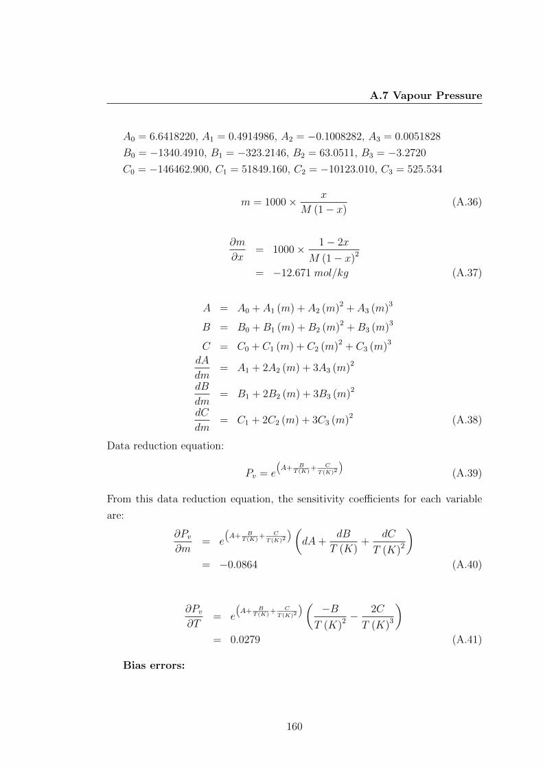
A.7 Vapour Pressure
A0 = 6.6418220, A1 = 0.4914986, A2 = −0.1008282, A3 = 0.0051828
B0 = −1340.4910, B1 = −323.2146, B2 = 63.0511, B3 = −3.2720
C0 = −146462.900, C1 = 51849.160, C2 = −10123.010, C3 = 525.534
m = 1000× x
M (1− x)(A.36)
∂m
∂x= 1000× 1− 2x
M (1− x)2
= −12.671 mol/kg (A.37)
A = A0 + A1 (m) + A2 (m)2 + A3 (m)3
B = B0 +B1 (m) +B2 (m)2 +B3 (m)3
C = C0 + C1 (m) + C2 (m)2 + C3 (m)3
dA
dm= A1 + 2A2 (m) + 3A3 (m)2
dB
dm= B1 + 2B2 (m) + 3B3 (m)2
dC
dm= C1 + 2C2 (m) + 3C3 (m)2 (A.38)
Data reduction equation:
Pv = e
(A+ B
T (K)+ C
T (K)2
)(A.39)
From this data reduction equation, the sensitivity coefficients for each variable
are:
∂Pv∂m
= e
(A+ B
T (K)+ C
T (K)2
)(dA+
dB
T (K)+
dC
T (K)2
)= −0.0864 (A.40)
∂Pv∂T
= e
(A+ B
T (K)+ C
T (K)2
)( −BT (K)2 −
2C
T (K)3
)= 0.0279 (A.41)
Bias errors:
160
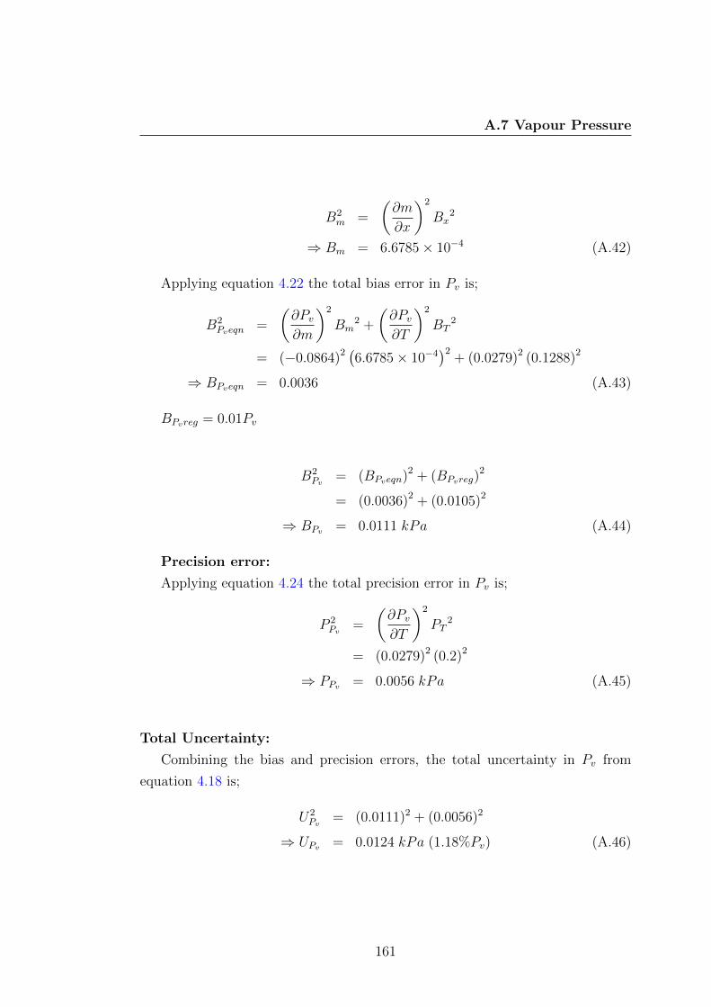
A.7 Vapour Pressure
B2m =
(∂m
∂x
)2
Bx2
⇒ Bm = 6.6785× 10⁻⁴ (A.42)
Applying equation 4.22 the total bias error in Pv is;
B2Pveqn =
(∂Pv∂m
)2
Bm2 +
(∂Pv∂T
)2
BT2
= (−0.0864)2 (6.6785× 10⁻⁴)2
+ (0.0279)2 (0.1288)2
⇒ BPveqn = 0.0036 (A.43)
BPvreg = 0.01Pv
B2Pv
= (BPveqn)2 + (BPvreg)2
= (0.0036)2 + (0.0105)2
⇒ BPv = 0.0111 kPa (A.44)
Precision error:
Applying equation 4.24 the total precision error in Pv is;
P 2Pv
=
(∂Pv∂T
)2
PT2
= (0.0279)2 (0.2)2
⇒ PPv = 0.0056 kPa (A.45)
Total Uncertainty:
Combining the bias and precision errors, the total uncertainty in Pv from
equation 4.18 is;
U2Pv
= (0.0111)2 + (0.0056)2
⇒ UPv = 0.0124 kPa (1.18%Pv) (A.46)
161

A.8 Piston Velocity
A.8 Piston Velocity
Piston Velocity, Vc [m/s]
Nominal value: 0.1003
Nominal input voltage: 8.2V
LDT output is between 4-20mA. A 250Ω resistor then converts this input to a
1 − 5V input to the data acquisition system. The output of sensor voltage as a
function of position was then used to determine a regression expression relating
these two parameters.
The equation relating piston axial position, xp[m] in terms of LDT output
voltage, Vo[V ];
xp = 0.0921947Vo − 0.0937527 (A.47)
For the nominal input voltage the linear curve fit for output voltage, Vo as a
function of time (sampling rate of 1000Hz) was determined to be;
Vo = 1.0777t+ 1.0018 (A.48)
Applying the chain rule, we can determine the piston velocity;
Vc =dxpdt
=dxpdVo
dVodt
(A.49)
Letting xV = dxpdVo
and Vo = dVodt
we can write
Vc = xV Vo (A.50)
Bias errors:
Bias in regression equation for xV (2Sr), BxV = 0.000655619 m/V
Bias in regression equation for Vo (2Sr), BVo= 0.027076 V/s
Applying equation 4.22 the total bias error in Vc is;
BVc2 =
(∂Vc∂xV
)2
B2xV
+
(∂Vc
∂Vo
)2
B2Vo
+2
(∂Vc∂xV
)(∂Vc
∂Vo
)B2xVB2Vo
= (1.0777)2(6.556× 10⁻⁴)2 + (0.0921947)2(0.027076)2
+2(1.0777)(0.0921947)(6.556× 10⁻⁴)(0.027076)
⇒ BVc = 3.204× 10⁻³ m/s (A.51)
162

A.9 Nozzle Velocity
Precision error:
Precision error in velocity (2Sr), PVc = 0.002134 m/s
Total Uncertainty:
Combining the bias and precision errors, the total uncertainty in Vc from
equation 4.18 is;
U2Vc = (0.003204)2 + (0.002134)2
⇒ UVc = 3.848× 10⁻³ m/s (A.52)
A.9 Nozzle Velocity
Nozzle Velocity, Vn [m/s]
Nominal value: 15.192
Piston velocity: 0.1003 m/s
Cylinder bore: 101.689× 10⁻³ m
Nozzle diameter: 8.246× 10⁻³ m
The equation relating nozzle velocity, Vn to piston velocity, Vc is;
Vn = Vc
(Dc
Dn
)2
(A.53)
where Dc and Dn represent the cylinder bore and nozzle diameters respectively.
From this data reduction equation, the sensitivity coefficients for each variable
are:
∂Vn∂Vc
=
(Dc
Dn
)2
= 152.076 (A.54)
∂Vn∂Dc
= 2VcDc
Dn2
= 299.998 1/s (A.55)
163

A.9 Nozzle Velocity
and
∂Vn∂Dn
= −2VcDc
2
Dn3
= −3699.55 1/s (A.56)
Bias errors:
Bias error in piston velocity (see section A.8), BVc = 3.204× 10⁻³ m/s
Bias error in cylinder bore diameter (see section A.2), BDc = 0.0635×10⁻³ m/s
Bias error in nozzle diameter (see section A.2), BDn = 0.05× 10⁻³ m/s
Applying equation 4.22 the total bias error in Vn is;
BVn2 =
(∂Vn∂Vc
)2
B2Vc +
(∂Vn∂Dc
)2
B2Dc
+
(∂Vn∂Dn
)2
B2Dn
= (152.076)2(3.204× 10⁻³)2 + (299.998)2(6.35× 10⁻⁵)2
+(−3699.55)2(5× 10⁻⁵)2
⇒ BVn = 0.5243 m/s (A.57)
Precision error:
Precision error in piston velocity (see section A.8), PVc = 0.002134 m/s
Precision error in nozzle diameter (see section A.2), PDn = 9.2× 10⁻⁶m
Applying equation 4.24 the total precision error in Vn is;
PVn2 =
(∂Vn∂Vc
)2
P 2Vc +
(∂Vn∂Dn
)2
P 2Dn
= (152.076)2(0.002134)2 + (−3699.55)2(9.2× 10⁻⁶)2
⇒ PVn = 0.3260 m/s (A.58)
Total Uncertainty:
Combining the bias and precision errors, the total uncertainty in Vn from
equation 4.18 is;
U2Vn = (0.5243)2 + (0.3260)2
⇒ UVn = 0.6164 m/s (4.06%Vn) (A.59)
164

A.10 Discharge Coefficient
A.10 Discharge Coefficient
Discharge Coefficient, Cd
Nominal value: 0.7756
Nominal Gas Pressure, P1: 458.313 kPa
Nominal Gas Pressure, P1: 95.863 kPa
Nominal density, ρ: 1871.2 kg/m3
Piston velocity, Vc: 0.1003 m/s
Cylinder bore, Dc: 101.689× 10⁻³ m
Nozzle diameter, Dn: 8.246× 10⁻³ m
Nominal ∆z: −0.202 m
Data reduction equation:
Cd =D2cVc
D2n√
1−β4
√2000(P1−P2)+ρg∆z
ρ
(A.60)
where β = Dn
Dp
From this data reduction equation, the sensitivity coefficients for each variable
are:
∂Cd∂Vc
=D2c
D2n√
1−β4
√2000(P1−P2)+ρg∆z
ρ
= 7.736 s/m (A.61)
∂Cd∂Dc
=2DcVc
D2n√
1−β4
√2000(P1−P2)+ρg∆z
ρ
= 15.223 1/m (A.62)
∂Cd∂Dn
=−2D2
cVc(D4n −D4
p (1− β4))
D4pD
3n
√1− β4
√2000(P1−P2)+ρg∆z
ρ
= 187.513 1/m (A.63)
165

A.10 Discharge Coefficient
∂Cd∂Dp
=2D2
cVcD2n
D3p
√1− β4
√2000(P1−P2)+ρg∆z
ρ
= 5.091× 10⁻⁵ 1/m (A.64)
∂Cd∂P1
=−1000D2
cVc√
1− β4
ρD2n
2000(P1−P2)+ρg∆zρ
3/2
= −0.0011 1/kPa (A.65)
∂Cd∂P2
=1000D2
cVc√
1− β4
ρD2n
2000(P1−P2)+ρg∆zρ
3/2
= 0.00111/kPa (A.66)
∂Cd∂ρ
=1000D2
cVc (P1 − P2)√
1− β4
D2nρ
2(
2000(P1−P2)+ρg∆zρ
) 32
= 2.078× 10⁻⁴ m3/kg (A.67)
and
∂Cd∂∆z
=−D2
cVcg√
1− β4
D2n
(2000(P1−P2)+ρg∆z
ρ
) 32
= −0.0197 1/m (A.68)
Bias errors:
Bias in piston velocity (see section A.9), BVc = 3.204× 10⁻³ m/s
Bias in cylinder bore (see section A.2), BDc = 6.35× 10⁻⁵ m
Bias in nozzle diameter (see section A.2), BDn = 5× 10⁻⁵ m
Bias in pipe diameter (see section A.2), BDp = 5× 10⁻⁵ m
Bias in injection pressure, P1 (see section A.1), BP1 = 13.84 kPa
Bias in gas pressure, P2 (see section A.1), BP2 = 4.03 kPa
Bias in density (see section A.6), Bρ = 6.093 kg/m3
166

A.11 Reynolds Number
Bias in ∆z (± half scale res.), B∆z = 5× 10⁻⁴ m
Applying equation 4.22 the total bias error in Cd is;
BCd
2 =
(∂Cd∂Vc
)2
B2Vc +
(∂Cd∂Dc
)2
B2Dc
+
(∂Cd∂Dn
)2
B2Dn
+
(∂Cd∂Dp
)2
B2Dp
+
(∂Cd∂P1
)2
B2P1
+
(∂Cd∂P2
)2
B2P2
+
(∂Cd∂ρ
)2
B2ρ +
(∂Cd∂∆z
)2
B2∆z
= (7.736)2(3.204× 10⁻³)2 + (15.223)2(6.35× 10⁻⁵)2 + (187.513)2(5× 10⁻⁵)2
+(5.091× 10⁻⁵)2(5× 10⁻⁵)2 + (−0.0011)2(13.84)2 + (0.0011)2(4.03)2
+(2.078× 10⁻⁴)2(6.093)2 + (−0.0197)2(5× 10⁻⁴)2
⇒ BCd= 0.0281 (A.69)
Precision error:
Precision error in discharge coefficient (2Sr), PCd= 0.0056 m/s
This was determined from the standard deviation of repeated injections at nom-
inally identical conditions. Total Uncertainty:
Combining the bias and precision errors, the total uncertainty in Cd from
equation 4.18 is;
U2Cd
= (0.0281)2 + (0.0056)2
⇒ UCd= 0.0286 (3.36%Cd) (A.70)
A.11 Reynolds Number
Reynolds Number, Re
Nominal value: 78631
Nominal nozzle velocity, Vn: 15.238 m/s
Nominal nozzle diameter, Dn: 8.246× 10⁻³ m
Nominal viscosity, ν: 1.598× 10⁻⁶ m2/s
167

A.11 Reynolds Number
Data reduction equation:
Re =VnDn
ν(A.71)
From this data reduction equation, the sensitivity coefficients for each variable
are:
∂Re
∂Vn=
Dn
ν= 5160.2 s/m (A.72)
∂Re
∂Dn
=Vnν
= 9.536× 10⁶ 1/m (A.73)
and
∂Re
∂ν= VnDn ln ν
= −1.6771 s/m2 (A.74)
Bias errors:
Bias in velocity (see section A.9), BVn = 0.5243 m/s
Bias in diameter (see section A.2), BDn = 0.05mm
Bias in viscosity (see section A.5), Bν = 0.0362× 10⁻⁶ m2/s
Applying equation 4.22 the total bias error in Re is;
BRe2 =
(∂Re
∂Vn
)2
B2Vn +
(∂Re
∂Dn
)2
B2Dn
+
(∂Re
∂ν
)2
B2ν
= (5160.2)2(0.5243)2 + (9.536× 10⁶)2(0.05)2 + (−1.6771)2(0.0362× 10⁻⁶)2
⇒ BRe = 2747.1 (A.75)
Precision error:
Precision error in velocity (see section A.9), PVn = 0.3260 m/s
Precision error in diameter (see section A.2), PDn = 9.2× 10⁻⁶m
168

A.12 Cavitation Number
Precision error in viscosity (see section A.5), Pν = 0.002× 10⁻⁶ m2/s
Applying equation 4.24 the total precision error in Re is;
PRe2 =
(∂Re
∂Vn
)2
P 2Vn +
(∂Re
∂Dn
)2
P 2Dn
+
(∂Re
∂ν
)2
P 2ν
= (5160.2)2(0.3260)2 + (9.536× 10⁶)2(9.2× 10⁻⁶)2 + (−1.6771)2(0.002× 10⁻⁶)2
⇒ PRe = 1684.4 (A.76)
Total Uncertainty:
Combining the bias and precision errors, the total uncertainty in Re from
equation 4.18 is;
U2Re = (2747.1)2 + (1684.4)2
⇒ URe = 3222.4 (4.098%Re) (A.77)
A.12 Cavitation Number
Cavitation number, K
Nominal value: 1.852
Nominal injection pressure, P1: 370.797 kPa
Nominal gas pressure, P2: 116.558 kPa
Nominal vapour pressure, Pv: 1.064 kPa
Nominal atmospheric pressure, Patm: 100.984 kPa
Data reduction equation:
K =(P1 + Patm)− Pv
P1 − P2
(A.78)
From this data reduction equation, the sensitivity coefficients for each variable
are:
∂K
∂Pv=
−1
P1 − P2
= −3.933× 10⁻³ 1/kPa (A.79)
169

A.13 Cavity Collapse Length
∂K
∂P1
=Pv − P2 − Patm
P1 − P22
= −3.349× 10⁻³ 1/kPa (A.80)
and
∂K
∂P2
=P1 + Patm − Pv
P1 − P22
= 7.284× 10⁻³ 1/kPa (A.81)
Bias errors:
Bias in vapour pressure (see section A.7), BPv = 0.011 kPa
Bias in injection pressure (see section A.1), BP1 = 13.84 kPa
Bias in gas pressure (see section A.1), BP2 = 4.03 kPa
Applying equation 4.22 the total bias error in K is;
BK2 =
(∂K
∂Pv
)2
B2Pv
+
(∂K
∂P1
)2
B2P1
+
(∂K
∂P2
)2
B2P2
= (−3.933× 10⁻³)2(0.011)2 + (−3.349× 10⁻³)2(13.84)2 + (7.284× 10⁻³)2(4.03)2
⇒ BK = 0.0164 (A.82)
Precision error:
Precision error in cavitation number (2Sr), PK = 0.0781 m/s
This was determined from the standard deviation of repeated injections at nom-
inally identical conditions.
Total Uncertainty:
Combining the bias and precision errors, the total uncertainty in K from
equation 4.18 is;
U2K = (0.0164)2 + (0.0781)2
⇒ UK = 0.0798 (A.83)
A.13 Cavity Collapse Length
Cavity collapse length was determined using the method outlined in section 4.3.1.
Cavity Collapse Length, Lcav/L
170

A.14 Shedding Frequency
Nominal value: 0.25
Bias errors:
Image resolution bias - (±1 pixel), Bres = 1.375× 10⁻³
Threshold conversion bias - estimated (±3 pixel), Bth = 4.125× 10⁻³
Entrance detection bias - estimated (±2 pixel), Bdet = 2.75× 10⁻³
Applying equation 4.22 the total bias error in Lcav/L is;
B2Lcav/L = B2
res +B2th +B2
det
= (1.375× 10⁻³)2 + (4.125× 10⁻³)2 + (2.75× 10⁻³)2
⇒ BLcav/L = 0.005 (A.84)
Precision error:
Standard deviation (2Sr), PLcav/L = 0.059
Total Uncertainty:
Combining the bias and precision errors, the total uncertainty in Lcav/L from
equation 4.18 is;
U2Lcav/L = (0.005)2 + (0.059)2
⇒ ULcav/L = 0.0592 (23.7%Lcav/L) (A.85)
A.14 Shedding Frequency
Periodic shedding frequency was determined using the method outlined in section
4.3.3.
Shedding Frequency, f [Hz]
Nominal value: 1600
Bias errors:
PSD resolution bias - (width of frequency bin), Bbin = 51.38
Precision error:
Standard deviation (2Sr), Pf = 3.87 Measured as the standard deviation of
the frequency determined for the individual interrogation points
Total Uncertainty:
171

A.15 Spray Angle
Combining the bias and precision errors, the total uncertainty in f from equa-
tion 4.18 is;
U2f = (51.38)2 + (3.87)2
⇒ Uf = 51.52 (3.22%f) (A.86)
A.15 Spray Angle
Spray angle was determined using the method outlined in section 4.3.2.
Spray Angle, θ []
Nominal value: 9.72
Bias errors:
Bias due to thresholding - (averaged from various trials), Bth = 0.75
Precision error:
Standard deviation (2Sr), Pθ = 1.012 Measured from repeated measurements
of the same image
Total Uncertainty:
Combining the bias and precision errors, the total uncertainty in θ from equa-
tion 4.18 is;
U2θ = (0.75)2 + (1.01)2
⇒ Uθ = 1.26 (12.96%θ) (A.87)
172

Appendix B
Instrumentation Calibration
Pressure Sensors
All pressure sensors used for this work was calibrated using a dead weight pressure
tester. Sensor output voltage was measured using the National Instruments PCI
6221 data acquisition card and TBX-68 I/O connector block to ensure end-to-
end calibration. Weights were gradually applied to the dead weight tester in
increments of 100 kPa equivalence. The entire process was repeated 3 times
for each sensor and the output voltages averaged to further reduce sample to
sample error. Figure B.1 shows the regression curve obtained for the gas pressure
sensor, while figure B.2 shows the regression curve obtained for the liquid injection
pressure sensor.
Thermocouples
Temperature measurements for ambient gas and liquid were measured using K-
type thermocouple probes located in measurement ports in the top of the pres-
sure vessel and in the supply pipe respectively. Calibration of these sensors was
conducted across a broad range of temperature and compared to a platinum
resistance thermometer. Figure B.3 shows the calibration curve for the gas tem-
perature thermocouple, while figure B.4 shows the calibration curve for the liquid
temperature thermocouple.
Piston velocity
Determination of the piston velocity require the linear position of the piston to
173

Sensor Output Voltage [V]
P1
[kP
a]
0 0.05 0.1 0.15 0.2 0.25 0.30
200
400
600
800
1000
1200
1400
1600
1800MeasuredPredicted
P2 = 5931.6V + 18.2
Figure B.1: Pressure vessel gas pressure sensor calibration
Sensor Output Voltage [V]
P1
[kP
a]
0 0.05 0.1 0.15 0.2 0.25 0.30
200
400
600
800
1000
1200
1400
1600
1800MeasuredPredicted
P1 = 6157.2V + 3.352
Figure B.2: Injection pressure sensor calibration
174

Platinum Reference, T - [oC]
Mea
sure
d T
emp,
T [o C
]
5 10 15 20 25 30 35 400
5
10
15
20
25
30
35
40
45
MeasuredPredicted
Tgas = 1.0057T - 0.2217
Figure B.3: Gas temperature thermocouple calibration
Platinum Reference, T - [oC]
Mea
sure
d T
emp,
T [o C
]
5 10 15 20 25 30 35 400
5
10
15
20
25
30
35
40
45
MeasuredPredicted
Tliq = 0.9937T + 0.3051
Figure B.4: Liquid temperature thermocouple calibration
175

be differentiated. The LDT generated an analog current output (4 − 20mA)
proportional to the piston position. This current output was input across a 250Ω
resistor to produce a range of output spanning 1−5V for the entire piston stroke
length. Figure B.5 shows the calibration of the piston position, measured as
distance in meters from zero position, against the converted LDT voltage. The
linear curve fit shows the expression relating these parameter. The relationship
predicting the piston velocity as a function of input voltage was then obtained
by applying the chain rule expression (see section A.8). The resulting curve was
then fit with a quadratic regression curve, as shown in figure B.6.
LDT Voltage, Vo [V]
Pis
ton
Pos
ition
, xp
[m]
1 1.2 1.4 1.6 1.8 2 20
0.02
0.04
0.06
0.08
0.1
0.12
MeasuredPredicted
xp = 0.0921947Vo - 0.0937527
Figure B.5: LDT piston position calibration
176

PCV Solenoid Voltage, V [V]
Pis
ton
Vel
ocity
, Vc c [
m/s
]
2 3 4 5 6 7 8 9 100
0.02
0.04
0.06
0.08
0.1
0.12
0.14
0.16MeasuredPredicted
Vc = 1.9676V2 - 3.6213V - 2.2683
Figure B.6: Piston velocity calibration
177

Appendix C
Pressure Vessel Drawings
As presented in Chapter 3, the design of an optical access pressure vessel formed
a major component of the development of the experimental rig used for this work.
The concept and design of the vessel was entirely conducted by the author, the key
features of which were discussed in section 3.5. Verification of material stresses
and fabrication of the vessel was completed by L & A Pressure Welding. Fur-
ther to this, registration of the pressure vessel with WorkCover NSW which is
a legal requirement for operation, required the design to be independently veri-
fied to comply to the regulations outlined in the Occupational Health and Safety
Regulation 2001. The design was found to comply to the Australian Standard
AS1210-1997 and registered with WorkCover NSW on 14/08/2009 - Registration
No: PV 6-120613/09.
The engineering drawings used for manufacture can be seen in the following
pages.
178

A A
150
N10
N3
N9
N8 N2
N5
N4
412
TORI
EN
D38
8 ID
X 1
2 PL
.4.
25 M
IN A
/F38
LO
NG
SF
BOTH
EN
DS
305
ICR
63.5
IKR
151
N5
N6
N10
N1
N7
110
0
90
180
270
45 135
225
315
DRI
LL &
TA
P M
16
ON
141
PC
D O
FF C
RS(4
OFF
)
165
180
270
0
90
163
LON
GITU
DIN
AL
SEA
M L
INE
ORI
ENTA
TION
125
N4
N7
N10
N2
N3
80.5
80.0
89
25
85 93 183
80
222.4
L
SEC
TION
A-A
SC
ALE
1 :
5NO
TE: I
TEM
S N
OT
IN S
ECTIO
N P
LAN
E HA
VE
BE
EN S
UPPR
ESSE
D F
OR
CLA
RITY
161
160
151
WEL
D S
EAM
NO
TE 3
4
2.7
R0.8
(typ
) DET
AIL
L
SCA
LE 1
: 1
ELEV
ATIO
NV
IEW
FRO
M 1
80 O
RIEN
TATIO
NEL
EVA
TION
VIE
W F
ROM
90
ORI
ENTA
TION
ORI
ENTA
TION
PLA
N -
VES
SEL
VIE
W F
ROM
TO
P O
F V
ESSE
L
ELEV
ATIO
NV
IEW
FRO
M 0
ORI
ENTA
TION
ORI
ENTA
TION
PLA
N -
VES
SEL
VIE
W F
ROM
BA
SE O
F V
ESSE
L
RL 8
76 T
AN
RL 5
76
RL 3
00
RL 0
.0 T
AN
302
301
401
601 70
2
701
= Ra
3.2
- R
a 6.
3 um
ALL
OV
ER=
ITEM
NUM
BER
= DE
TAIL
NUM
BER
1. SY
MBO
LS :-
FP
NOTES = M
EDIU
M M
ACH
INE,
Ra
3.2
- Ra
6.3
um
= FU
LL P
ENET
RATI
ON
2. W
ELD
S :-
DET
AIL
DRA
WIN
GS
OF
WEL
D T
YPES
CA
N B
E FO
UND
ON
DRA
WIN
G S
HEET
10.
3. N
OZZ
LE N
ECK
TO S
HELL
WEL
D -
SEA
L W
ELD
GRI
ND
FLU
SH
DES
IGN
DA
TAD
esig
n Pr
essu
re1.
5 M
PaD
esig
n Te
mpe
ratu
re65
C to
-5C
Hyd
ro. T
est P
ress
ure
2.26
MPa
Cor
rosio
n A
llow
ance
0 m
mP.
W.H
.Tnl
lRa
dio
grap
hynl
lHa
zard
Lev
elC
D E FC
12
34
BA
32
15
C D
46
78
A B
01
Cam
eron
Sta
nley
WEI
GHT
:
A3
SHEE
T 1 O
F 10
SCA
LE:1
:20
DW
G N
O.
TITLE
:
REV
ISIO
N:
7D
O N
OT
SCA
LE D
RAW
ING
DA
TE:
CO
NTA
CT
DEB
UR A
ND
BRE
AK
SHA
RP E
DG
ES
APP
V'D
Ph:
DRA
WN
UNSW PR
ESSU
RE V
ESSE
L
13/0
8/09
UNLE
SS O
THER
WIS
E SP
ECIF
IED:
DIM
ENSI
ON
S A
RE IN
MM
SURF
AC
E FI
NIS
H:
TOLE
RAN
CES
: 0.
5(0
2) 9
385
6005
Figure C.1: Pressure vessel - drawing sheet 1
179

NO
TES: ITE
M 1
71 IS
TO
BE
SUPP
LIED
BY
UNSW
AN
D T
HEN
1.
WEL
DED
TO
ITEM
164
BY
L&A
AC
CO
RDIN
G T
O
DRA
WIN
G 0
9.2.
E
LEV
ATIO
N O
F N
OZZ
LES
IS M
EASU
RED
FRO
M T
HE
BO
TTO
M S
HELL
-HEA
D C
IRC
UMFE
REN
TIAL
WEL
D
S
EAM
.3.
E
LEV
ATIO
N F
OR
NO
ZZLE
N10
IS M
EASU
RED
TO
THE
FLA
NG
E FA
CE.
BILL
OF
MA
TERI
ALS
ITEM
DES
CRI
PTIO
NQ
TYM
ATE
RIA
L SP
ECIF
ICA
TION
150
CYL
IND
RIC
AL
SHEL
L -
412
OD
x 8
00 L
G x
12
PL.
1A
STM
A24
0-30
415
1TO
RI H
EAD
- 41
2 O
D x
38
S.F.
X 1
2 PL
.2
AST
M A
240-
304
152
N1-
N3
NEC
K - 8
0 N
B SC
H 40
S x
184
LG3
AST
M A
312-
TP30
415
3N
1-N
3 FL
AN
GE
- 23
0 O
D x
91
ID x
32
PL.
3A
STM
A24
0-30
415
4N
1-N
9 BL
IND
- 23
0 O
D x
16
PL.
9A
STM
A24
0-30
415
5N
1-N
9 SI
GHT
GLA
SS -
169
OD
x 1
7 TH
K9
BORO
SILI
CA
TE15
6N
4-N
9 N
ECK
- 100
NB
SCH
40S
x 76
LG
6A
STM
A31
2-TP
304
157
N4-
N9
FLA
NG
E -
230
OD
x
116
ID x
32
PL.
6A
STM
A24
0-30
415
8N
1-N
9 G
ASK
ET -
169
OD
x
143
ID x
1.5
THK
18C
NA
F15
9N
1-N
9 HE
X HE
AD
BO
LTS
AN
D N
UTS
- M16
x 1
20 L
G.
72A
STM
A19
3-B7
M/A
STM
A19
4M-2
H16
0N
10 N
ECK
- 80
NB
SCH
40S
x 75
LG
.1
AST
M A
312-
TP30
416
1N
10 F
LAN
GE
- 18
3 O
D x
91
ID x
25
PL.
1A
STM
A24
0-30
416
2N
10 G
ASK
ET (O
-RIN
G -
92.1
5 O
D x
3.1
5 W
IDE)
1V
ITON
163
GA
S PO
RT -
1" B
SP H
ALF
CO
UPLI
NG
, 300
# 1
2A
STM
A18
2-F3
0416
4PI
PE F
LAN
GE
- 18
3 O
D x
63
ID x
32
PL.
1A
STM
A24
0-30
416
5PI
PE P
ORT
- 3/
8" B
SP, 3
000#
HA
LF C
OUP
LIN
G2
AST
M A
182-
F304
166
NO
ZZLE
INSE
RT F
LAN
GE
- 18
3 O
D x
50
ID x
32
PL.
1A
STM
A24
0-30
416
7PI
PE P
ORT
- 1/
4" B
SP, 3
000#
HA
LF C
OUP
LIN
G1
AST
M A
182-
F304
168
LIFT
ING
LUG
- 10
PL.
x 7
5 x
110
2A
STM
A24
0-30
416
9LI
FTIN
G L
UG P
AD
- 10
PL.
x 1
10 X
315
1A
STM
A24
0-30
417
0N
AM
ING
PLA
TE B
RAC
KET
- 6 P
L. x
175
x 4
301
AST
M A
240-
304
171
SUPP
LY P
IPE
- 50N
B SC
H 40
S**
1A
STM
A31
2-TP
304
172
MO
UNTIN
G B
RAC
KET
PAD
- 10
PL.
x 2
50 x
270
2A
STM
A24
0-30
417
3M
OUN
TING
BRA
CKE
T LU
G -
10 P
L. x
150
x 3
502
AST
M A
240-
304
REF
RL E
LEV
ATIO
NO
RIEN
TATIO
NO
DID
POSI
TION
SHE
LL/H
EAD
HORI
ZON
TAL/
VER
TICA
LN
1-4
20
88.9
77.9
HEA
DHO
RIZO
NTA
LN
2-4
290
88.9
77.9
HEA
DHO
RIZO
NTA
LN
3-4
227
088
.977
.9HE
AD
HORI
ZON
TAL
N4
135
315
114.
310
2.26
SHEL
LHO
RIZO
NTA
LN
513
545
114.
310
2.26
SHEL
LHO
RIZO
NTA
LN
613
522
511
4.3
102.
26SH
ELL
HORI
ZON
TAL
N7
350
011
4.3
102.
26SH
ELL
HORI
ZON
TAL
N8
350
9011
4.3
102.
26SH
ELL
HORI
ZON
TAL
N9
350
270
114.
310
2.26
SHEL
LHO
RIZO
NTA
LN
10-1
84.4
-88
.980
HEA
DV
ERTIC
AL
D E FC
12
34
BA
32
15
C D
46
78
A B
02
Cam
eron
Sta
nley
WEI
GHT
:
A3
SHEE
T 2
OF
10SC
ALE
:1:2
0
DW
G N
O.
TITLE
:
REVI
SIO
N:
6D
O N
OT
SCA
LE D
RAW
ING
DA
TE:
CO
NTA
CT
DEB
UR A
ND
BRE
AK
SHA
RP E
DG
ES
APP
V'D
Ph:
DRA
WN
UNSW
BILL
OF
MA
TERI
ALS
13/0
8/09
UNLE
SS O
THER
WIS
E SP
ECIF
IED:
DIM
ENSI
ON
S A
RE IN
MM
SURF
AC
E FI
NIS
H:
TOLE
RAN
CES
: 0.
5(0
2) 9
385
6005
Figure C.2: Pressure vessel - drawing sheet 2
180

250
250
50
62
MO
UNTIN
G B
RAC
KET
DET
AIL
TOP
WEL
D S
EAM
150
120
R280
100
18 H
ole
fo
r M16
anch
or b
olt0
5ty
p
5ty
p
5ty
p5
140
50
50
10
150
163
2 O
FF
1" B
SP
DET
AIL
172
173
TOP
WEL
D S
EAM
102
301
FILL
ING
PO
RT
DET
AIL
302
RL 5
76
D E FC
12
34
BA
32
15
C D
46
78
A B
03
Cam
eron
Sta
nley
WEI
GHT
:
A3
SHEE
T 3
OF
10SC
ALE
:1:2
0
DW
G N
O.
TITLE
:
REV
ISIO
N:
4D
O N
OT
SCA
LE D
RAW
ING
DA
TE:
CO
NTA
CT
DEB
UR A
ND
BRE
AK
SHA
RP E
DG
ES
APP
V'D
Ph:
DRA
WN
UNSW
MO
UNTIN
G B
RAC
KET
15/0
6/09
UNLE
SS O
THER
WIS
E SP
ECIF
IED:
DIM
ENSI
ON
S A
RE IN
MM
SURF
AC
E FI
NIS
H:
TOLE
RAN
CES
: 0.
5(0
2) 9
385
6005
Figure C.3: Pressure vessel - drawing sheet 3
181

R37.5
150
75
75
50
22 H
ole
10 P
L.16
8
300
110
10 PL.
R10 (
typ) C
C
1" B
SP2
OFF
169
6FP
5
SEC
TION
C-C
SC
ALE
1 :
5
NO
TE: T
HE V
IEW
ON
THE
LEF
T IS
A C
ROPP
ED V
IEW
.
DET
AIL
S O
F TH
E N
OZZ
LES
AN
D O
THER
FEA
TURE
S O
UT
O
F PL
AN
E HA
VE
BEEN
SUP
PRES
SED
FO
R C
LARI
TY.
401
LIFT
ING
LUG
DET
AIL
D E FC
12
34
BA
32
15
C D
46
78
A B
04
Cam
eron
Sta
nley
WEI
GHT
:
A3
SHEE
T 4
OF
10SC
ALE
:1:2
0
DW
G N
O.
TITLE
:
REV
ISIO
N:
4D
O N
OT
SCA
LE D
RAW
ING
DA
TE:
CO
NTA
CT
DEB
UR A
ND
BRE
AK
SHA
RP E
DG
ES
APP
V'D
Ph:
DRA
WN
UNSW LI
FTIN
G L
UGS
15/0
6/09
UNLE
SS O
THER
WIS
E SP
ECIF
IED:
DIM
ENSI
ON
S A
RE IN
MM
SURF
AC
E FI
NIS
H:
TOLE
RAN
CES
: 0.
5(0
2) 9
385
6005
Figure C.4: Pressure vessel - drawing sheet 4
182

5
50 20 7 TYP.
210
5
5
1455
740
6050
28
DESI
GN P
RESS
.
RADI
OGRA
PHY
HAZ.
LEV
EL (A
S 43
43)
L. &
A. P
ress
ure
Wel
ding
Pty
Ltd
CORR
OSIO
N A
LLOW
.
WEI
GHT
EMPT
Y
INSP
ECTO
R ID
VOL
UME
:::
DESI
GN C
ODE
APP
ROV
AL
NO.
ORDE
R NO
.SE
RIA
L NO
.
QA
S NO
.::::
ITEM
NA
ME
ITEM
NO.
:::
kg cu.m
TEST
DA
TEPW
HT
CODE
CLA
SS
AS
1210
- 1
997
QEC
058
2HO
LDTE
ST P
RESS
.
DESI
GN T
EMP.
REV
ESBY
SYDN
EY
P.LA.
.
:HO
LD::::::::
kPag
kPag
mm
°C
N.S.
W.
UNSW
RES
EARC
H PR
ESSU
RE V
ESSE
L
317
0.12
3
1500
50 0 2260
2BC
NIL
NIL
4 HO
LES
5
- TEX
T TO
BE
ETC
HED
AN
D B
LAC
K EN
AM
ELED
- TITL
E TE
XT 2
.5M
M H
IGH,
DA
TA T
EXT
4MM
HIG
H
SCA
LE -
3:4
(1 R
EQUI
RED)
NAMEPLATE
D E FC
12
34
BA
32
15
C D
46
78
A B
05
Cam
eron
Sta
nley
WEI
GHT
:
A3
SHEE
T 5
OF
10SC
ALE
:1:2
0
DW
G N
O.
TITLE
:
REVI
SIO
N:
5D
O N
OT
SCA
LE D
RAW
ING
DA
TE:
CO
NTA
CT
DEB
UR A
ND
BRE
AK
SHA
RP E
DG
ES
APP
V'D
Ph:
DRA
WN
UNSW
NA
ME
PLA
TE
22/0
7/09
UNLE
SS O
THER
WIS
E SP
ECIF
IED:
DIM
ENSI
ON
S A
RE IN
MM
SURF
AC
E FI
NIS
H:
TOLE
RAN
CES
: 0.
5(0
2) 9
385
6005
Figure C.5: Pressure vessel - drawing sheet 5
183

262D
D
N
WEL
D S
EAM
LON
GITU
DIN
AL
SEA
M L
INE
ORI
ENTA
TION
125
O
SEC
TION
D-D
SC
ALE
1 :
10
20135
175
250
25 DET
AIL
N
SCA
LE 1
: 5
170
4 O
FF 5 HO
LES
6
R16
50
DET
AIL
O
SCA
LE 1
: 5
6TY
P
601
NA
MIN
G P
LATE
BRA
CKE
TD
ETA
IL
RL 3
00
D E FC
12
34
BA
32
15
C D
46
78
A B
06
Cam
eron
Sta
nley
WEI
GHT
:
A3
SHEE
T 6
OF
10SC
ALE
:1:2
0
DW
G N
O.
TITLE
:
REV
ISIO
N:
4D
O N
OT
SCA
LE D
RAW
ING
DA
TE:
CO
NTA
CT
DEB
UR A
ND
BRE
AK
SHA
RP E
DG
ES
APP
V'D
Ph:
DRA
WN
UNSW
NA
ME
PLA
TE B
RAC
KET
15/0
6/09
UNLE
SS O
THER
WIS
E SP
ECIF
IED:
DIM
ENSI
ON
S A
RE IN
MM
SURF
AC
E FI
NIS
H:
TOLE
RAN
CES
: 0.
5(0
2) 9
385
6005
Figure C.6: Pressure vessel - drawing sheet 6
184
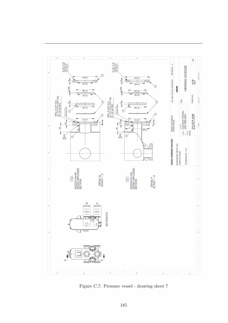
E E
PQ
SEC
TION
E-E
63
32
170
17
168
1.5
THK
142
168
16
142
230
9
230
DET
AIL
P
SCA
LE 1
: 5
153
154
155
5 M
AX
from
fille
tw
eld
leg
to su
rface
DRI
LL &
TA
P M
16on
191
PC
D O
FF C
RSFi
t 159
(8 O
FF)
152
8 O
FF
18HO
LES
ON
19
1 PC
D6 6
230
14216
168
142
1.5
THK
17
168
170
932
63
DET
AIL
Q
SCA
LE 1
: 5
154
157
155
5 M
AX
from
fille
t w
eld
leg
to su
rface
DRI
LL &
TA
P M
16on
191
PC
D O
FF C
RSFi
t 159
(8 O
FF)
156
158
8 O
FF
18HO
LES
ON
19
1 PC
D
6 6
158
NO
ZZLE
N1-
N3
DET
AIL
EXP
LOD
EDSE
CTIO
N
NO
ZZLE
N4-
N9
DET
AIL
EXP
LOD
EDSE
CTIO
N 701
702
D E FC
12
34
BA
32
15
C D
46
78
A B
07
Cam
eron
Sta
nley
WEI
GHT
:
A3
SHEE
T 7
OF
10SC
ALE
:1:2
0
DW
G N
O.
TITLE
:
REV
ISIO
N:
5D
O N
OT
SCA
LE D
RAW
ING
DA
TE:
CO
NTA
CT
DEB
UR A
ND
BRE
AK
SHA
RP E
DG
ES
APP
V'D
Ph:
DRA
WN
UNSW
VIE
WIN
G N
OZZ
LES
22/0
7/09
UNLE
SS O
THER
WIS
E SP
ECIF
IED:
DIM
ENSI
ON
S A
RE IN
MM
SURF
AC
E FI
NIS
H:
TOLE
RAN
CES
: 0.
5(0
2) 9
385
6005
Figure C.7: Pressure vessel - drawing sheet 7
185

F
F
32 PL.
50
58
66
81
183
25
R
SEC
TION
F-F
4 O
FF
18 h
oles
on 1
41 P
CD
Fit M
16 B
olts
166
42.7
R0.8 (TYP)
DET
AIL
R
SCA
LE 1
: 1
Ra 3
.2
D E FC
12
34
BA
32
15
C D
46
78
A B
08
Cam
eron
Sta
nley
WEI
GHT
:
A3
SHEE
T 8
OF
10SC
ALE
:1:2
DW
G N
O.
TITLE
:
REV
ISIO
N:
4D
O N
OT
SCA
LE D
RAW
ING
DA
TE:
CO
NTA
CT
DEB
UR A
ND
BRE
AK
SHA
RP E
DG
ES
APP
V'D
Ph:
DRA
WN
UNSW
NO
ZZLE
INSE
RT F
LAN
GE
15/0
6/09
UNLE
SS O
THER
WIS
E SP
ECIF
IED:
DIM
ENSI
ON
S A
RE IN
MM
SURF
AC
E FI
NIS
H:
TOLE
RAN
CES
: 0.
5(0
2) 9
385
6005
Figure C.8: Pressure vessel - drawing sheet 8
186

G G
H
H0 18
0
270
315
58
66
183
85
55
100
S
SEC
TION
G-G
50 N
B SC
H XS
164
1/4"
-18
NPT
x 2
0 m
in
167
165
3/8"
BSP
P x
20 m
in
(25 afte
r machining)
32 PL.
SEC
TION
H-H
4 O
FF
18ho
les o
n 14
1 PC
D
9 6 6
FP
4
R0.8 (t
yp)
2.7
3
DET
AIL
S
SCA
LE 1
: 1
90
135
O-R
ING
GRO
OV
E
D E FC
12
34
BA
32
15
C D
46
78
A B
09
Cam
eron
Sta
nley
WEI
GHT
:
A3
SHEE
T 9
OF
10SC
ALE
:1:5
DW
G N
O.
TITLE
:
REVI
SIO
N:
5D
O N
OT
SCA
LE D
RAW
ING
DA
TE:
CO
NTA
CT
DEB
UR A
ND
BRE
AK
SHA
RP E
DG
ES
APP
V'D
Ph:
DRA
WN
UNSW
NO
ZZLE
FLA
NG
E BE
LOW
A
CRY
LIC
NO
ZZLE
22/0
7/09
UNLE
SS O
THER
WIS
E SP
ECIF
IED:
DIM
ENSI
ON
S A
RE IN
MM
SURF
AC
E FI
NIS
H:
TOLE
RAN
CES
: 0.
5(0
2) 9
385
6005
Figure C.9: Pressure vessel - drawing sheet 9
187

3
0 - 1.5
6
6
5 m
ax
6 6
6
13
12
10
0 TO
3
1.5 - 2.5
50° M
IN
3
0 - 1.5
1001
FP
60°
NOT
TO S
CALE
INSI
DE
CIR
CUM
FERE
NTIA
L SE
AM
WEL
D
N10
NO
ZZLE
NEC
KTO
FLA
NG
E W
ELD
NOT
TO S
CALE
N1-
N9
NO
ZZLE
NEC
KTO
FLA
NG
E W
ELD
NOT
TO S
CALE
SOC
KET
TO H
EAD
WEL
D
NOT
TO S
CALE
INSI
DE
NOT
TO S
CALE
LON
GITU
DIN
AL
SEA
M W
ELD
1002
INSI
DE
NECK
NOT
TO S
CALE
R3
6FP
NO
ZZLE
TO
SH
ELL/
HEA
D W
ELD
1003
1004
1005
1006
SEE
NO
TE 1
SEE
NO
TE 2
SEE
NO
TE 3
SEE
NO
TE 4
SEE
NO
TE 5
SEE
NO
TE 6
NO
TES: Sing
le-w
eld
ed si
ngle
V b
utt j
oint
as p
er
1.A
S121
0 FI
GUR
E 3.
5.1.
5 (A
) (f)
Dou
ble-
wel
ded
sing
le V
but
t joi
nt a
s per
2.A
S121
0 FI
GUR
E 3.
5.1.
5 (A
) (g)
Wel
d a
s per
AS1
210
FIG
URE
3.19
.3 (B
)(f)
3.
Wel
d a
s per
AS1
210
FIG
URE
3.21
.3 (b
)4.
Wel
d a
s per
AS1
210
FIG
URE
3.21
.3 (j
)5.
Wel
d a
s per
AS1
210
FIG
URE
3.19
.4 (g
)6.
60°
D E FC
12
34
BA
32
15
C D
46
78
A B
10
Cam
eron
Sta
nley
WEI
GHT
:
A3
SHEE
T 10
OF
10SC
ALE
:1:2
0
DW
G N
O.
TITLE
:
REV
ISIO
N:
4D
O N
OT
SCA
LE D
RAW
ING
DA
TE:
CO
NTA
CT
DEB
UR A
ND
BRE
AK
SHA
RP E
DG
ES
APP
V'D
Ph:
DRA
WN
UNSW W
ELD
DET
AIL
S
13/0
8/09
UNLE
SS O
THER
WIS
E SP
ECIF
IED:
DIM
ENSI
ON
S A
RE IN
MM
SURF
AC
E FI
NIS
H:
TOLE
RAN
CES
: 0.
5(0
2) 9
385
6005
Figure C.10: Pressure vessel - drawing sheet 10
188
Appendix D
Hydraulic Equipment
The propulsion of liquid through the test section was accomplished using hy-
draulic cylinders, as described in Chapter 3. All hydraulic components used for
this work were purchased from Parker Hannifin Australia. Where possible stan-
dard hydraulic components were used. Special attention was given to the corro-
sive properties of the Sodium Iodide test fluid, which required the test cylinder
to be manufactured from Stainless Steel and use non-standard piston seals. A
Schematic showing the arrangement of the hydraulic system and a list of key
components can be seen in figure D.1.
As mentioned in section 3.4 the cylinder end-cap for the test fluid cylinder
was customed designed by the author to minimise the flow separation in the
contraction from the cylinder bore to the supply piping entry. Figure D.2 shows
the engineering drawing of this end cap.
189

Figure D.1: Hydraulic System Schematic
190

Figure D.2: Test Fluid Cylinder End Cap
191

References
Afzal, H., Arcoumanis, C., Gavaises, M. & Kampanis, N. (1999). Inter-
nal flow in diesel injector nozzles - modelling and experiments. Proc. IMechE
Seminar on Fuel Injection Systems , London, 25–44. 26, 34, 35
Andriotis, A., Gavaises, M. & Arcoumanis, C. (2008). Vortex flow and
cavitation in diesel injector nozzles. Journal of Fluid Mechanics , 610, 195–215.
35
Arai, M., Tabata, M., Hiroyasu, H. & Shimizu, M. (1984). Disintegrating
process and spray characterisation of fuel jet injected by a diesel nozzle. SAE
Technical Paper , 840275. 18, 22, 28
Arcoumanis, C. & Gavaises, M. (1998). Cavitation in diesel injectors: mod-
elling and experiments. In Proc. ILASS-Europe, 248–255. 26
Arcoumanis, C. & Whitelaw, J. (2002). Is cavitation improtant in diesel
engine injectors? 145–159. 27
Arcoumanis, C., Flora, H., Gavaises, M., Kampanis, N. & Horrocks,
R. (1999). Investigation of cavitation in a vertical multi-hole injector. SAE
Technical Paper , 1999-01-0524. 24, 27, 34
Arcoumanis, C., Badami, M., Flora, H. & Gavaises, M. (2000). Cav-
itation in real-size multi-hole diesel injector nozzles. SAE Technical Paper ,
2000-01-1249. 27, 35
192

REFERENCES
Arndt, R., Song, C., Kjeldsen, M., He, J., Keller, A. et al. (2000).
Instability of partial cavitation: a numerical/experimental approach. In 23rd
Symposium on Naval Hydrodynamics, September, Rouen, France. 41
Asi, O. (2006). Failure of a diesel engine injector nozzle by cavitation damage.
Engineering Failure Analysis , 13, 1126–1133. 36
Badock, C., Wirth, R., Fath, A. & Leipertz, A. (1999). Investigation of
cavitation in real size diesel injection nozzles. International Journal of Heat
and Fluid Flow , 20, 538–544. 24, 26
Bae, C., Yu, J., Kang, J., Kong, J. & Ook Lee, K. (2002). Effect of
nozzle geometry on the common-rail diesel spray. SAE Technical Paper , 2002-
01-1625. 2
Benajes, J., Pastor, J., Payri, R. & Plazas, A. (2004). Analysis of the
influence of diesel nozzle geometry in the injection rate characteristics. Journal
of Fluids Engineering , Vol. 126, 63–71. 28, 33
Berger, S., Talbot, L. & Yao, L. (1983). Flow in curved pipes. Annual
Review of Fluid Mechanics , 15, 461–512. 59
Bergwerk, W. (1959). Flow pattern in diesel nozzle spray holes. Proc Inst Mech
Eng , 173, 655–660. 26
Billet, M. (1985). Cavitation nuclei measurements-a review. In Proc. 1985
ASME Cavitation and Multiphase Flow Forum, 31–38. 8
Billet, M. & Holl, J. (1981). Scale effects on various types of limited cavita-
tion. Journal of Fluids Engineering , 103, 405. 27
Blaker, A. (1965). Photography for Scientific Publication - A Handbook . W. H.
Freeman and Company. 81
Blessing, M., Konig, G., Kruger, C., Michels, U. & Schwarz, V.
(2003). Analysis of flow and cavitation phenomena in diesel injection nozzles
and its effects on spray and mixture formation. In Two day conference on fuel
193

REFERENCES
injection systems: organized by the Combustion Engines and Fuels Group of the
Automobile Division of the Institution of Mechanical Engineers (IMechE), vol.
610, 21, Professional Engineering for the Institution of Mechanical Engineers.
35, 36
Brandner, P., Walker, G., Niekamp, P. & Anderson, B. (2007). An
investigation of cloud cavitation about a sphere. 16th Australasian Fluid Me-
chanics Conference (AFMC), 1392–1398. 41
Brennen, C. (1995). Cavitation and bubble dynamics . Oxford University Press.
5, 7, 27, 35
Budwig, R. (1994). Refractive index matching methods for liquid flow investi-
gations. Experiments in fluids , 17, 350–355. 70
Bunnell, R., Heister, S., Yen, C. & Collicott, S. (1999). Cavitating
injector flows: validation of numerical models and simulations of pressure at-
omizers. Atomization and Sprays , 9, 445–465. 42
Callenaere, M., Franc, J., MICHEL, J. & Riondet, M. (2001). The
cavitation instability induced by the development of a re-entrant jet. Journal
of Fluid Mechanics , 444, 223–256. 36, 37, 39, 113, 131
Castleman, R. (1932). The mechanism of atomization accompanying solid in-
jection. N.A.C.A, Report No. 440. 15, 16
Chandra, B. & Collicott, S. (1999). Experimental investigation of cavita-
tion frequency in a slot orifice. 12th Annual conference of ILASS, Americas ,
379–383. 41, 127
Chaves, H., Knapp, M., Kubitzek, A., Obermeier, F. & Schneider, T.
(1995). Experimental study of cavitation in the nozzle hole of diesel injectors
using transparent nozzles. SAE Technical Paper , 950290. 24, 25, 26, 28, 139
Chen, R. & Fan, L. (1992). Particle image velocimetry for characterizing the
flow structure in three-dimensional gas-liquid-solid fluidized beds. Chemical
Engineering Science, 47, 3615–3622. 71
194

REFERENCES
Coleman, H. & Steele, W. (1995). Engineering application of experimental
uncertainty analysis. AIAA journal , 33, 1888–1896. 96
Coleman, H. & Steele, W. (1999). Experimentation and uncertainty analysis
for engineers . Wiley-Interscience. 96
Coutier-Delgosha, O., Stutz, B., Vabre, A. & Legoupil, S. (2007).
Analysis of cavitating flow structure by experimental and numerical investiga-
tions. Journal of Fluid Mechanics , 578, 171. 39
Dan, T., Yamamoto, T., Senda, J. & Fujimoto, H. (1997). Effect of
nozzle configurations for characteristics of non-reacting diesel fuel spray. SAE
transactions , 106, 581–596. 26
Daugherty, R. & Franzini, J. (1965). Fluid mechanics with engineering ap-
plications . McGraw-Hill, 6th edn. 109
De Lange, D. & De Bruin, G. (1998). Sheet cavitation and cloud cavitation,
re-entrant jet and three-dimensionality. Applied scientific research, 58, 91–114.
42, 113
De Lange, D., Bruin, G. & Wijngaarden, L. (1994). On the mechanism of
cloud cavitation - experiment and modelling. The 2nd international symposium
on Cavitation, Tokyo, Japan, 45–49. 40, 122
DeJuhasz, K. (1931). Dispersion of sprays in solid injection oil engines. Trans.
ASME Oil and Gas Power . 17
Desantes, J., Pastor, J. & Doudou, A. (2001). Study of the steady flow
produced by direct injection diesel engine intake ports. Proc Inst Mech Eng,,
215, 285 – 298. 28
Desantes, R., J.M. and, Salvador, F. & Gil, A. (2006). Development
and validation of a theoretical model for diesel spray penetration. Fuel , 85,
910–917. 87
Dodge, L., Ryan III, T. & M.G, R. (1992). Effects of different injector hole
shapes on diesel sprays. SAE Technical Paper , 920623. 19, 23
195

REFERENCES
Dumont, N., Simonin, O. & Habchi, C. (2000). Cavitating flow in diesel
injectors and atomization: a bibliographic review. Proceedings of the 8th In-
ternational Conference on Liquid Atomization and Spray Systems , Pasadena,
California. 28
Duttweiler, M. & Brennen, C. (1998). Partial cavity instabilities. US-Japan
Seminar on Abnormal Flow Phenomena in Turbomachines, Osaka, Japan. 40,
122
Franc, J. & Michel, J. (2004). Fundamentals of Cavitation. Springer. 5, 7,
27
Ganippa, L., Bark, G., Andersson, S. & Chomiak, J. (2004). Cavitation:
a contributory factor in the transition from symmetric to asymmetric jets in
cross-flow nozzles. Experiments in Fluids , 36, 627–634. 29
Gavaises, M. (2008). Flow in valve covered orifice nozzles with cylindrical and
tapered holes and link to cavitation erosion and engine exhaust emissions.
International Journal of Engine Research, 9, 435–447. 36
Gavaises, M. & Andriotis, A. (2006). Cavitation inside multi-hole injectors
for large diesel engines and its effect on the near-nozzle spray structure. SAE
Technical Paper , 2006-01-1114. 35
Gavaises, M., Papoulias, D., Andriotis, A., Giannadakis, E. &
Theodorakakos, A. (2007). Link between cavitation development and ero-
sion damage in diesel fuel injector nozzles. SAE Technical paper , 2007–01–0246.
35
Gavaises, M., Andriotis, A., Papoulias, D., Mitroglou, N. &
Theodorakakos, A. (2009). Characterization of string cavitation in large-
scale diesel nozzles with tapered holes. Physics of Fluids , 21, 052107. 3, 35,
36
Gelalles, A. (1930). Effect of orifice length-diameter ratio on spray character-
istics. N.A.C.A, Technical Note No. 352. 15
196

REFERENCES
Gelalles, A. (1932). Coefficients of discharge of fuel injection nozzles for
compression-ignition engines. N.A.C.A, Report No. 373. 15
Giffen, E. & Muraszew, A. (1953). The Atomization of Liquid Fuels . John
Wiley and Sons, Inc., NY. 1
Haenlein, A. (1932). Disintegration of a liquid jet. N.A.C.A, Technical Mem-
orandum No. 659. 16
He, L. & Ruiz, F. (1995). Effect of cavitation on flow and turbulence in plain
orifices for high-speed atomization. Atomization and Sprays , 5, 569–584. 28
Henry, M. & Collicott, S. (2000). Visualization of internal flow in a cavi-
tating slot orifice. Atomization and Sprays , 10, 545–563. 26
Hiroyasu, H. (1991). Experimental and theoretical studies on the structure of
fuel sprays in diesel engines. proceedings of the International Conference on
Liquid Atomization and Spray Systems (ICLASS 91), Gaithersburg, Mary-
land, 15-18 July, 17–31. 4
Hiroyasu, H. (2000). Spray breakup mechanism from the hole-type nozzle and
its applications. Atomization and Sprays , 10, 511–527. 26, 135
Hiroyasu, H., Shimizu, M. & Arai, M. (1982). The breakup of high speed
jet in a high pressure gaseous atmosphere. Proceedings of ICLASS-82 . 18
Hiroyasu, H., Arai, M. & Shimizu, M. (1991). Break-up length of a liquid
jet and internal flow in a nozzle. Proceedings of the International Conference on
Liquid Atomization and Spray Systems (ICLASS 91), Gaithersburg, Mary-
land, 15-18 July, 275–282. 22, 26, 28
Ito, H. (1960). Pressure losses in smooth pipe bends. J. Basic Eng , 82, 43. 59
Iyer, V. & Abraham, J. (1997). Penetration and dispersion of transient gas
jets and sprays. Combustion Science and Technology , 130, 315–334. 21
197

REFERENCES
Joussellin, F., Delannoy, Y., Sauvage-Boutar, E. & Goirand, B.
(1991). Experimental investigations on unsteady attached cavities. ASME
FED , 116, 61–66. 38
Karasawa, T., Tanaka, M., Abe, K., Shiga, S. & Kurabayashi, T.
(1992). Effect of nozzle configuration on the atomization of a steady spray.
Atomization and Sprays , vol 2, 411–426. 19, 20
Kawanami, Y., Kato, H., Yamaguchi, H., Tanimura, M. & Tagaya, Y.
(1997). Mechanism and control of cloud cavitation. Journal of fluids engineer-
ing , 119, 788. 38, 39, 41, 119
Kent, J. & Brown, G. (1982). Nozzle exit flow characteristics for square-
edged and rounded inlet geometries. Combustion Science and Technology , 30,
121–132. 19, 20
Kim, J., Nishida, K., Yoshizaki, T. & Hiroyasu, H. (1997). Characteriza-
tion of flows in the sac chamber and the discharge hole of a d.i. diesel injection
nozzle by using a transparent model nozzle. SAE Technical Paper , 972942.
34, 35
Kline, S. & McClintock, F. (1953). Describing uncertainties in single-sample
experiments. Mechanical engineering , 75, 3–8. 98
Knapp, R. (1955). Recent investigations of the mechanics of cavitation and
cavitation damage. Trans. ASME , 77, 1045–1054. 36, 37
Knapp, R. (1957). Investigation of the Mechanics of Cavitation and Cavitation
Damage. California Institute of Technology, Hydrodynamics Laboratory. 35
Knapp, R., Daily, J. & Hammitt, F. (1970). Cavitation. McGraw-Hill New
York. 5
Knox-Kelecy, A. (1992). Turbulent Flow in a Scale Model of a Diesel Fuel
Injector Nozzle Hole. Ph.D. thesis, University of Wisconsin. 21
Knox-Kelecy, A. & Farrell, P. (1992). Internal flow in a scale model of a
diesel fuel injector nozzle. SAE Technical paper , 922308. 21
198

REFERENCES
Knox-Kelecy, A. & Farrell, P. (1993). Spectral characteristics of turbulent
flow in a scale model of a diesel fuel injector nozzle. SAE Technical Paper ,
930924. 21
Kubota, A., Kato, H., Yamaguchi, H. & Maeda, M. (1989). Unsteady
structure measurement of cloud cavitation on a foil section using conditional
sampling technique. Journal of fluids engineering , 111, 204–210. 37, 40
Kuehn, R. (1925). Atomization of liquid fuels. N.A.C.A, T.M. Nos. 329, 330,
331. 15, 16
Laberteaux, K. & Ceccio, S. (2001a). Partial cavity flows. part 1. cavities
forming on models without spanwise variation. Journal of Fluid Mechanics ,
431, 1–41. 39
Laberteaux, K. & Ceccio, S. (2001b). Partial cavity flows. part 2. cavities
forming on test objects with spanwise variation. Journal of Fluid Mechanics ,
431, 43–63. 40
Lauterborn, W. & Ohl, C. (1997). The peculiar dynamics of cavitation
bubbles. Applied scientific research, 58, 63–76. 82
Le, Q., Franc, J. & Michel, J. (1993). Partial cavities: global behavior and
mean pressure distribution. Journal of fluids engineering , 115, 243–248. 37,
38, 40, 113, 116, 119, 127
Lee, D. (1933). The effect of nozzle design and operating conditions on the
atomization and distribution of fuel sprays. N.A.C.A, Report No. 425. 15,
21
Lee, D. & Spencer, R. (1934). Photomicrographic studies of fuel sprays.
N.A.C.A, Report No. 454. 15, 16
Lefebvre, A. (1989). Atomization and sprays (Combustion: An International
Series). Hemisphere Publishing Corporation. 1
Leroux, J. (2004). An experimental study of unsteady partial cavitation. Jour-
nal of fluids engineering , 126, 94. 39, 41
199

REFERENCES
Leroux, J., Coutier-Delgosha, O. & Astolfi, J. (2005). A joint experi-
mental and numerical study of mechanisms associated to instability of partial
cavitation on two-dimensional hydrofoil. Physics of Fluids , 17, 052101. 39
Lichtarowicz, A., Duggins, R. & Markland, E. (1965). Discharge coef-
ficients for incompressible non-cavitating flow through long orifices. Journal
Mechanical Engineering Science, Vol 7, 210–219. 32, 58, 109, 132
Lim, W., Chew, Y., Chew, T. & Low, H. (1994). Particle image velocimetry
in the investigation of flow past artificial heart valves. Annals of biomedical
engineering , 22, 307–318. 72
Marcer, R. & Legouez, J. (2001). Simulation of unsteady cavitating flows
in diesel injector with an improved VOF-method. In Proc of 17th ILASS-Eu
Conf . 19
McCarthy, M. & Molloy, N. (1974). Review of stability of liquid jets and
the influence of nozzle design. The Chemical Engineering Journal , 7, 1–20. 18,
22
McKenney, E. & Brennen, C. (1994). On the dynamics and acoustics of
cloud cavitation on an oscillating hydrofoil. In ASME , 190, 195–202, American
Society of Mechanical Engineers. 39
Miller, H. & Beardsley, E. (1926). Spray penetration with a simple fuel
injection nozzle. NACA, Report No. 222. 15, 21
Miller, P., Danielson, K., Moody, G., Slifka, A., Drexler, E. &
Hertzberg, J. (2006). Matching index of refraction using a diethyl phtha-
late/ethanol solution for in vitro cardiovascular models. Experiments in Fluids ,
41, 375–381. 70, 72
Mirchandani, G. (2011). Spectral analysis in matlab - part ii. Laboratory notes
for Digital Signal Processing, The University of Vermont . 90
Narrow, T., Yoda, M. & Abdel-Khalik, S. (2000). A simple model for the
refractive index of sodium iodide aqueous solutions. Experiments in Fluids , 28,
282–283. 71
200

REFERENCES
Nouri, J., Mitroglou, N., Yan, Y. & Arcoumanis, C. (2007). Internal
flow and cavitation in a multi-hole injector for gasoline direct-injection engines.
SAE Technical Paper , 2007-01-1405. 35
Nurick, W. (1976). Orifice cavitation and its effect on spray mixing. Journal of
Fluids Engineering , 98, 681–687. 13, 31, 132, 133
Ohrn, T., Senser, D. & Lefebvre, A. (1991a). Geometric effects on spray
cone angle for plain-orifice atomizers. Atomization and Sprays , Vol 1, 253–268.
19, 23
Ohrn, T., Senser, D. & Lefebvre, A. (1991b). Geometrical effects on dis-
charge coefficients for plain-orifice atomizers. Atomization and Sprays , 1. 33
Patil, K., Tripathi, A., Pathak, G. & Katti, S. (1991). Thermodynamic
properties of aqueous electrolyte solutions. 2. Vapor pressure of aqueous solu-
tions of sodium bromide, sodium iodide, potassium chloride, potassium bro-
mide, potassium iodide, rubidium chloride, cesium chloride, cesium bromide,
cesium iodide, magnesium chloride, calcium chloride, calcium bromide, cal-
cium iodide, strontium chloride, strontium bromide, strontium iodide, barium
chloride, and barium bromide. Journal of Chemical and Engineering Data, 36,
225–230. 75
Payri, F., Bermudez, V., Payri, R. & Salvador, F. (2004). The influence
of cavitation on the internal flow and the spray characteristics in diesel injection
nozzles. Fuel , 83, 419–431. 28, 33, 87, 133
Payri, R., Garcia, J., Salvador, F. & Gimeno, J. (2005). Using spray
momentum flux measurements to understand the influence of diesel nozzle ge-
ometry on spray characteristics. Fuel , Vol. 84, 551–561. 33
Payri, R., Salvador, F., Gimeno, J. & Zapata, L. (2008). Diesel noz-
zle geometry influence on spray liquid-phase fuel penetration in evaporative
conditions. Fuel , 87, 1165–1176. 33
201

REFERENCES
Pearce, I. & Lichtarowicz, A. (1971). Discharge performance of long orifices
with cavitating flow. In Proceedings of the 2nd Fluid Power Symposium, vol. 2,
13–35. 30, 31
Pham, T., Larrarte, F. & Fruman, D. (1999). Investigation of unsteady
sheet cavitation and cloud cavitation mechanisms. Journal of fluids engineer-
ing , 121, 289. 38, 119
Plateau, J. (1945). Statique experimentale et theorique des liquides soumis aux
seules forces moleculaires. In L. Rayleigh, ed., Theory of Sound , vol. Vol. II,
Dover, New York. 15
Plesset, M. (1949). The dynamics of cavitation bubbles. Trans. ASME J. Appl.
Mechanics , 16, 228–231. 11
Ramamurthi, K. & Patnaik, S. (2002). Influence of periodic disturbances
on inception of cavitation in sharp-edged orifices. Experiments in Fluids , 33,
720–727. 26
Ramamurthi, K., Nandakumar, K., Shankar, S. & Patnaik, R. (2001).
Hysteresis and bifurcation of flow in fuel injector nozzles. Proc Inst Mech Eng ,
215, 49–59. 26, 135
Randall, L. (1952). Rocket applications of the cavitating venturi. American
Rocket Society Journal , January-February, 28–31. 31
Randall, R. (1987). Frequency Analysis . Bruel & Kjær, 3rd edn. 91
Ranz, W. (1958). Some experiments on orifice sprays. Can J. Chem. Engng ,
August, 175–181. 17
Ray, S. (2002). High speed photography and photonics . SPIE - The International
Society for Optical Engineering. 82
Rayleigh, L. (1917). On the pressure development in a liquid during the collapse
of a spherical cavity. Phil. Mag., Vol. 34, pp. 94–98. 11, 15
202

REFERENCES
Reese, J., Chen, R. & Fan, L. (1995). Three-dimensional particle image
velocimetry for use in three-phase fluidization systems. Experiments in Fluids ,
19, 367–378. 71
Reisman, G. & Brennen, C. (1996). Pressure pulses generated by cloud cav-
itation. Proc. ASME Symp. on Cavitation and Gas-Liquid Flows in Fluid Ma-
chinery and Devices. FED Vol. 236 , 319–328. 39
Reisman, G., Wang, Y. & Brennen, C. (1998). Observations of shock waves
in cloud cavitation. Journal of Fluid Mechanics , 355, 255–283. 39, 41
Reitz, R. & Bracco, F. (1979a). On the dependence of spray angle and other
spray parameters on nozzle design and operating conditions. SAE Technical
Paper . 22, 28
Reitz, R. & Bracco, F. (1979b). Ultra-high-speed filming of atomizing jets.
Physics of Fluids , 22, 1054. 22
Reitz, R.D. & Bracco, F. (1982). Mechanisms of atomization of a liquid jet.
Phys. Fluids , 25, 1730–1742. 16, 17, 18, 19, 21, 22
Roth, H., Gavaises, M. & Arcoumanis, C. (2002). Cavitation initiation,
its development and link with flow turbulence in diesel injector nozzles. SAE
TRANSACTIONS , 111, 561–580. 29, 35
Roth, H., Giannadakis, E., Gavaises, M., Arcoumanis, C., Omae, K.,
Sakata, I., Nakamura, M. & Yanagihara, H. (2005). Effect of multi-
injection strategy on cavitation development in diesel injector nozzle holes.
SAE transactions , 114, 1029–1045. 35
Ruiz, F. (1991). A few useful relations for cavitating orifices. Proceedings of the
International Conference on Liquid Atomization and Spray Systems (ICLASS
91), Gaithersburg, Maryland, 15-18 July, 595–602. 33
Ruiz, F. & He, L. (1999). Turbulence Under Quasi-cavitating Conditions: A
New Species? Atomization and Sprays , 9, 419–430. 28
203

REFERENCES
Sakoda, M., Yakushiji, R., Maeda, M. & Yamaguchi, H. (2001). Mech-
anism of cloud cavitation generation on a 2-d hydrofoil. In 4th International
Symposium on Cavitation. 38
Sato, K. & Saito, Y. (2002). Unstable cavitation behavior in a circular-
cylindrical orifice flow. JSME International Journal Series B , 45, 638–645.
38, 40, 41, 42, 103, 107, 108, 127
Schlichting, H. (1968). Boundary-layer theory . McGraw-Hill, 6th edn. 58, 109
Schmidt, D. & Corradini, M. (1997). Analytical prediction of the exit flow
of cavitating orifices. Atomization and Sprays , Vol. 7, 603–616. 33
Schmidt, D. & Corradini, M. (2001). The internal flow of diesel fuel injector
nozzles: a review. Int. J. Engine Research, Vol. 2, 1–22. 22, 23, 33
Schmidt, D., Su, T.F., Goney, K., Farrell, P. & Corradini, M. (1995).
Detection of cavitation in fuel injector nozzles. In 8th ISTP Conference, San
Francisco, California, 1521–1532. 33
Schweitzer, P.H. (1937). Mechanism of disintegration of liquid jets. Journal
of Applied Physics , 8, 513–521. 17
Soteriou, C., Andrews, R. & Smith, M. (1995). Direct injection diesel
sprays and the effect of cavitation and hydraulic flip on atomization. SAE
Technical Paper , 950080. 24, 28, 31, 33, 34, 139
Soteriou, C., Andrews, R. & Smith, M. (1999). Further studies of cavita-
tion and atomization in diesel injection. SAE Technical Paper , 1999-01-1486.
24, 25, 61
Sou, A., Hosokawa, S. & Tomiyama, A. (2006). Cavitation in a two-
dimensional nozzle and liquid jet atomization. JSME Internation Journal , Se-
ries B, 49, 1253 –1259. 28, 29
Sou, A., Hosokawa, S. & Tomiyama, A. (2007). Effects of cavitation in
a nozzle on liquid jet atomisation. International Journal of Heat and Mass
Transfer , 50, 3575–3582. 29, 129, 139
204

REFERENCES
Sou, A., Maulana, M., Hosokawa, S. & Tomiyama, A. (2008). Ligament
formation induced by cavitation in a cylindrical nozzle. Journal of Fluid Science
and Technology , 3, 633–644. 29
Sou, A., Hosokawa, S. & Tomiyama, A. (2010). Cavitation in nozzles of
plain orifice atomizers with various length-diameter-ratios. Atomization and
Sprays , 20. 85
Spikes, R. & Pennington, G. (1959). Discharge coefficient of small submerged
orifices. Proceedings of the Institution of Mechanical Engineers , 173, 661–674.
30, 31
Stern, F., Muste, M., Beninati, M. & Eichinger, W. (1999). Summary
of Experimental Uncertainty Assessment Methodology with Example. IIHR
Report, Iowa Institute of Hydraulic Research, The University of Iowa, Iowa
City, IA. 96
Stutz, B. & Reboud, J. (1997a). Experiments on unsteady cavitation. Exper-
iments in fluids , 22, 191–198. 39, 127
Stutz, B. & Reboud, J. (1997b). Two-phase flow structure of sheet cavitation.
Physics of Fluids , 9, 3678. 39
Sugimoto, Y. & Sato, K. (2009). Visualization of unsteady behavior of cav-
itation in circular cylindrical orifice with abruptly expanding part. The 13th
International Topical Meeting on Nuclear Reactor Thermal Hydraulics . 38, 42
Suh, H.K., Park, S.H. & Lee, C.S. (2008). Experimental investigation of
nozzle cavitating flow characteristics for diesel and biodiesel fuels. International
Journal of Automotive Technology , 9, 217–224. 26
Tamaki, N., Shimizu, M., Nishida, K. & Hiroyasu, H. (1998). Effects of
cavitation and internal flow on atomization of a liquid jet. Atomization and
Sprays , 3, pp.179–197. 28
Taylor, G. (1963). Generation of ripples by wind blowing over a viscous fluid.
The Scientific Papers of G.I. Taylor , Vol. 3. 16
205

REFERENCES
Uzol, O., Chow, Y., Katz, J. & Meneveau, C. (2002). Unobstructed
particle image velocimetry measurements within an axial turbo-pump using
liquid and blades with matched refractive indices. Experiments in Fluids , 33,
909–919. 71, 73
Wade, R. & Acosta, A. (1966). Experimental observations on the flow past a
plano-convex hydrofoil. ASME J. Basic Eng , 88, 273–283. 37
Weber, C. (1931). Disintegration of liquid jets. Z. Angew. Math. Mech., 11,
136–154. 15
Welch, P. (1967). The use of fast fourier transform for the estimation of power
spectra: a method based on time averaging over short, modified periodograms.
Audio and Electroacoustics, IEEE Transactions on, 15, 70–73. 92
Wu, K., Reitz, R. & Bracco, F. (1986). Measurements of drop size at the
spray edge near the nozzle in atomizing liquid jets. Physics of Fluids , 29, 941.
22
Wu, K.J., Su, C.C., Steinberger, R., Santavicca, D. & Bracco, F.
(1983). Measurement of the spray angle of atomizing jets. Trans. ASME J.
Fluids Eng., Ser. I, 406–413. 18, 27, 28
Young, W. & Budynas, R. (2002). Roark’s Formulas for Stress and Strain.
London: McGrath-Hill, New York, 7th edn. 53
206


![NUMERICAL INVESTIGATION OF CAVITATING FLOW IN …annals.fih.upt.ro/pdf-full/2018/ANNALS-2018-2-24.pdfnozzles [7,8], from cavitation inception through partial cavitation, full cavitation](https://img.pdfslide.net/doc/110x75/608fbf7c5ef46b0f1e060437/numerical-investigation-of-cavitating-flow-in-nozzles-78-from-cavitation-inception.jpg)