Master of Science Thesis KTH School of Industrial Engineering and Management

Energy Technology EGI-2015-102MSC EKV1121 Division of Heat and Power Technology

SE-100 44 STOCKHOLM

Experimental loss measurements in an annular sector cascade at

supersonic exit velocities

László Lilienberg

-2-

Master of Science Thesis EGI 2015-102MSC EKV1121

Experimental loss measurements in an annular sector cascade at supersonic exit

velocities

László Lilienberg

Approved

04.01.2016

Examiner

Paul Petrie-Repar

Supervisor

Jens Fridh Commissioner

Contact person

-3-

Abstract

Efficiency improvement is one of the most important aspects of engineering and especially important in the field of energy production. In the past decades, energy was mostly produced by fossil based technologies involving turbomachines, and the efficiency of these machines nearly quadrupled since the introduction of the first economically viable gas turbines. The progress continues, as there are still areas where improvement can be made. Such area is the High Pressure Turbine stage (HPT), which influences the flow characteristics and losses downstream, which this thesis will examine in more detail.

In the open literature it can be found that one of the areas with potential for progress is the external cooling of the nozzle guide vanes (NGV) of the HPT stage. However not many studies go towards supersonic exit velocities even though that is the most common trend followed by the industry these days. The external cooling allows the turbine entry temperature (TET) to go beyond the melting point of the blade material thus increase Carnot efficiency but in the meantime influences the flow characteristics and losses. To understand these influences of the cooling, experiments in an annular sector cascade (ASC) were conducted with exit velocities from Mach 0.95 to 1.2 without and with cooling applied. The findings of the experiments are believed to help the more detailed understanding of the flow behaviour at high exit velocities.

When comparing the corresponding runs in the two cases it became obvious that with cooling applied the deviation of the exit flow angle is generally smaller than in the uncooled case. This might be a highly important design feature for designers to work with. From the available data it was concluded that the total pressure distribution across the span is not significantly affected with the introduction of cooling.

-4-

Table of Contents

Abstract ........................................................................................................................................................................... 3

LIST OF FIGURES ..................................................................................................................................................... 5

LIST OF TABLES ........................................................................................................................................................ 7

NOMENCLATURE .................................................................................................................................................... 9

1 Introduction ........................................................................................................................................................ 10

1.1 State-of-the-art Secondary Flow ............................................................................................................. 11

1.2 State-of-the-art Aerodynamic Losses ..................................................................................................... 13

1.3 Shockwave Losses and Boundary Layer Interaction ........................................................................... 16

1.4 State-of-the-art in External Cooling ....................................................................................................... 18

1.5 Research motivation ................................................................................................................................. 21

1.6 Objectives ................................................................................................................................................... 22

1.7 Methodology .............................................................................................................................................. 22

1.7.1 Literature study ................................................................................................................................. 22

1.7.2 Probe calibration .............................................................................................................................. 23

1.7.3 Assemble the test rig ....................................................................................................................... 23

1.7.4 Run periodicity trials ........................................................................................................................ 23

1.7.5 Uncooled Case Measurements ....................................................................................................... 23

1.7.6 Cooled Case Measurements ........................................................................................................... 23

1.7.7 Data evaluation ................................................................................................................................. 23

1.8 Research Limitations ................................................................................................................................ 24

2 Experimental approach ..................................................................................................................................... 25

2.1 NGV Geometry and Cascade Arrangement ......................................................................................... 25

2.2 Description of the Rig, Cascade Arrangement and Measuring Equipment .................................... 27

2.3 Calibration of the Measurement Probe ................................................................................................. 31

3 Periodicity Trials ................................................................................................................................................. 36

4 Uncooled Measurements................................................................................................................................... 41

5 External Cooling Measurements ...................................................................................................................... 49

6 Concluding Remarks .......................................................................................................................................... 59

7 Future work ......................................................................................................................................................... 60

Bibliography ................................................................................................................................................................. 61

8 Appendixes .......................................................................................................................................................... 63

8.1 Appendix A Uncertainty Analysis .......................................................................................................... 63

8.2 Appendix B Details of Area Traverse .................................................................................................... 64

-5-

LIST OF FIGURES

Figure 1-1 Industrial gas turbine SGT5-8000H 10

Figure 1-2 Increase of the thermal cycle efficiency through pressure ratio and TET over the last decades 11

Figure 1-3 Streamlines showing separation lines in a near endwall plane of a linear blade passage 12

Figure 1-4 Passage and horseshoe vortexes 13 Figure 1-5 Spanwise loss distribution at different Mach numbers 17 Figure 1-6 Spanwise exit flow angle distribution at different Mach numbers 18 Figure 1-7 Display of cooling hole configurations on a NGV 19 Figure 1-8 Reaction between main stream and coolant flow 19 Figure 1-9 Jet to the main flow from a single cooling hole 20 Figure 1-10 Boundary layer pattern for different momentum-flux ratios 21

Figure 2-1 Scheme of profile geometric parameters 25 Figure 2-2 Cooling holes on NGV 26 Figure 2-3 Cooling hole locations on the NGV 27 Figure 2-4 Schematic picture of the air supply system and the test rig 27 Figure 2-5 ASC Arrangement 28 Figure 2-6 ASC radial view 28 Figure 2-7 Axial cross section of ASC 29 Figure 2-8 Aeroprobe 30 Figure 2-9 Aeroprobe front view 30 Figure 2-10 Grid of measurement points 31 Figure 2-11 Calibration nozzle 32 Figure 2-12 Calibration coefficient plots for Mach 0.8 33 Figure 2-13 Normalised pressure comparison at pitch 0° at Mach 0.8 34 Figure 2-14 K1 Coefficient for KTH at Mach 0.8 34 Figure 2-15 K1 Coefficient for Aeroprobe at Mach 0.8 35

Figure 3-1 Estimated Mach number distribution across the ASC at M 095 36 Figure 3-2 Estimated Mach number periodicity at M 095 37 Figure 3-3 Estimated Mach number distribution across the ASC at M 1.05 37 Figure 3-4 Estimated Mach number periodicity at M 1.05 38 Figure 3-5 Estimated Mach number distribution across the ASC at M 1.15 38 Figure 3-6 Estimated Mach number periodicity at M 1.15 39 Figure 3-7 Estimated Mach number distribution across the ASC at M 1.20 39 Figure 3-8 Estimated Mach number periodicity at M 1.20 40

Figure 4-1 Total pressure distribution at Mach 0.95 uncooled case 41 Figure 4-2 Mass averaged kinetic energy loss Mach 0.95 uncooled case 42 Figure 4-3 Area averaged exit flow angle Mach 0.95 uncooled case 42 Figure 4-4 Mach number distribution at Mach 0.95 uncooled case 43 Figure 4-5 Total pressure distribution at Mach 1.05 uncooled case 44 Figure 4-6 Mass averaged kinetic energy loss Mach 1.05 uncooled case

-6-

Figure 4-7 Area averaged exit flow angle Mach 1.05 uncooled case 45 Figure 4-8 Mach number distribution at Mach 1.05 uncooled case Figure 4-9 Total pressure distribution at Mach 1.15 uncooled case Figure 4-10 Mass averaged kinetic energy loss Mach 1.15 uncooled case Figure 4-11 Area averaged exit flow angle Mach 1.15 uncooled case 46 Figure 4-12 Mach number distribution at Mach 1.15 uncooled case 46 Figure 4-13 Total pressure distribution at Mach 1.20 uncooled case 47 Figure 4-14 Mass averaged kinetic energy loss Mach 1.20 uncooled case Figure 4-15 Area averaged exit flow angle Mach 1.20 uncooled case 48 Figure 4-16 Mach number distribution at Mach 1.20 uncooled case

Figure 5-1 Total pressure distribution at Mach 0.95 cooled case 50 Figure 5-2 Mass averaged kinetic energy loss Mach 0.95 cooled case Figure 5-3 Area averaged exit flow angle Mach 0.95 cooled case 51 Figure 5-4 Mach number distribution at Mach 0.95 cooled case 52 Figure 5-5 Total pressure distribution at Mach 1.05 cooled case 53 Figure 5-6 Mass averaged kinetic energy loss Mach 1.05 cooled case Figure 5-7 Area averaged exit flow angle Mach 1.05 cooled case 53 Figure 5-8 Mach number distribution at Mach 1.05 cooled case 54 Figure 5-9 Total pressure distribution at Mach 1.15 cooled case 55 Figure 5-10 Area averaged exit flow angle Mach 1.15 cooled case Figure 5-11 Area averaged exit flow angle Mach 1.15 cooled case 55 Figure 5-12 Mach number distribution at Mach 1.15 cooled case 56 Figure 5-13 Total pressure distribution at Mach 1.20 cooled case 57 Figure 5-14 Mass averaged kinetic energy loss Mach 1.20 cooled case Figure 5-15 Area averaged exit flow angle Mach 1.20 cooled case 57 Figure 5-16 Mach number distribution at Mach 1.20 cooled case 58

Figure 9-1 Definition of pitch and yaw angle (adapted from Pütz, 2010) 64

Figure 9-2 Yaw and pitch angles defined by five-hole probe (left), front view of the 5-hole probe head 65

Figure 9-3 Traverse system (Glodic, 2008) 66

-7-

LIST OF TABLES

Table 2-1 Geometric parameters of NGV 25 Table 2-2 Cooling geometric information 26 Table 2-3 Position of measurement points 29

Table 5-1 Cooling hole configuration 49 Table 5-2 Total and NGV0 mass flows for different exit Mach numbers 49

Table 8-1 Measurement equipment and their inaccuracies 63

-8-

-9-

NOMENCLATURE

Latin Symbols m Mass flow [kg/s]

u Velocity [m/s] h Specific Enthalpy [kJ/kg] Y Mass-flux ratio [%] M Mach number [-] T Temperature [K] p Pressure [Pa] R Gas constant [J/(kg*K)] BR Blowing ratio [-] MR Momentum flux ratio [-] DR Density ratio [-]

Greek Symbols η Efficiency [-]

φ Velocity coefficient [-] κ Specific heat capacity ratio [-] ρ Density [kg/m3] φ Radial traverse angles [°]

Subscripts c Coolant

iso Isentropic st Static 1 Upstream 2 Downstream m Mainstream t Total

Abbreviations ASC Annular Sector Cascade

TET Turbine Entry Temperature NGV Nozzle Guide Vane CFD Computational Fluid Dynamics LE Leading Edge TE Trailing Edge SH Shower head SS Suction side PS Pressure side HPT High Pressure Turbine

-10-

1 Introduction

An excessive growth in industrialization and transport resulted in higher demand for energy than ever before. Since the conventional energy production relies mostly on fossil based fuels, implementing more efficient technologies is not only essential to save fuel but to reduce CO2 emissions and its impact on global warming (Saha, R. 2014). The worlds energy supply in 2012 was relying 81.7% on fossil based fuels from which 21.3% was natural gas (IEA. 2014). Gas turbines are turbomachines usually supplied by fossil based fuels and used for convert these fuels into usable power (Figure 1-1). They can be found in aviation, marine technologies and of course in mainland power generation. They are mostly used for their high power density, which means they can have the same power output from smaller size than other power generating appliances. Due to these practicalities and the facts that the demand for air transportation and shale gas extraction becoming more and more important the gas turbine industry faces a bright future.

Figure 1-1: Industrial gas turbine SGT5-8000H (Courtesy of Siemens)

From an industry point of view the role of research and development is to create more competitive technology which materializes in the cutback of capital and operational costs. Contraction of operating costs in gas turbines means achieving better efficiencies through reduced specific fuel consumption. Efficiency improvements came a long way since the first economically viable gas turbine with the thermal efficiency around 17.4% (Hunt, R. 2011) while todays machines can go up to around 60% (Hada, et al., 2012). To achieve these, there is a continuous push from the industry towards higher exit velocities and higher total entry temperature (TET). Increasing the TET has its physical limitations in the melting points of the materials but influences the thermal efficiency positively (Figure 1-2). Increasing the exit velocity,

-11-

results in higher pressure difference between the static and the total pressure of the flow and in highly loaded turbine stages which is more suitable at the moment. Increasing the TET can only be achieved by implementing internal and external cooling and even using these methods it is hard to push further than around 1800 K. Increasing the total pressure results in higher specific enthalpy which is directly proportional to the power output.

Figure 1-2: Increase of the thermal cycle efficiency through pressure ratio and TET over the last decades (Birch, N. T.,

2000.)

Nowadays trend is to reduce the vane count and thus reduce the weight, material and cooling air needed and the future trends aim for short height and long chord blades which will have a larger impact on secondary flow losses. This aligns with the increase of the exit velocity of the flow and it also increases the secondary flow losses across the NGV which are playing key parts in the efficiencies of the turbine. Present studies’ contribution to the field is to investigate the magnitude of the losses and their effect on the turbine efficiencies. Current experiment was conducted with exit isentropic Mach numbers between 0.95 up to 1.2.

1.1 State-of-the-art Secondary Flow By the definition of Lakshminarayana and Horlock (1963) “Within a blade passage in a cascade, a deflection of the low momentum fluid equal to the mainstream deflection would not be sufficient to obtain the balance between the pressure gradients and the centrifugal forces. As a result the low momentum fluid is turned more than the mainstream. In a cascade this deviation from the uniformly deflected stream is the secondary flow” By the definition of D. R. Glynn and H. Marsh (1980) “The term 'secondary flow' is usually associated with the small, velocity components across the blade passage and along the span of the blades which are produced by the turning of a shear flow in a cascade.” Because the relationship between the mainstream and the secondary flow is really complex not even mentioning the added trickiness with the cooling flow introduced to accurately simulate a flow like this with a CFD technique is impossible for now even with the strongest computers in the world. To describe

-12-

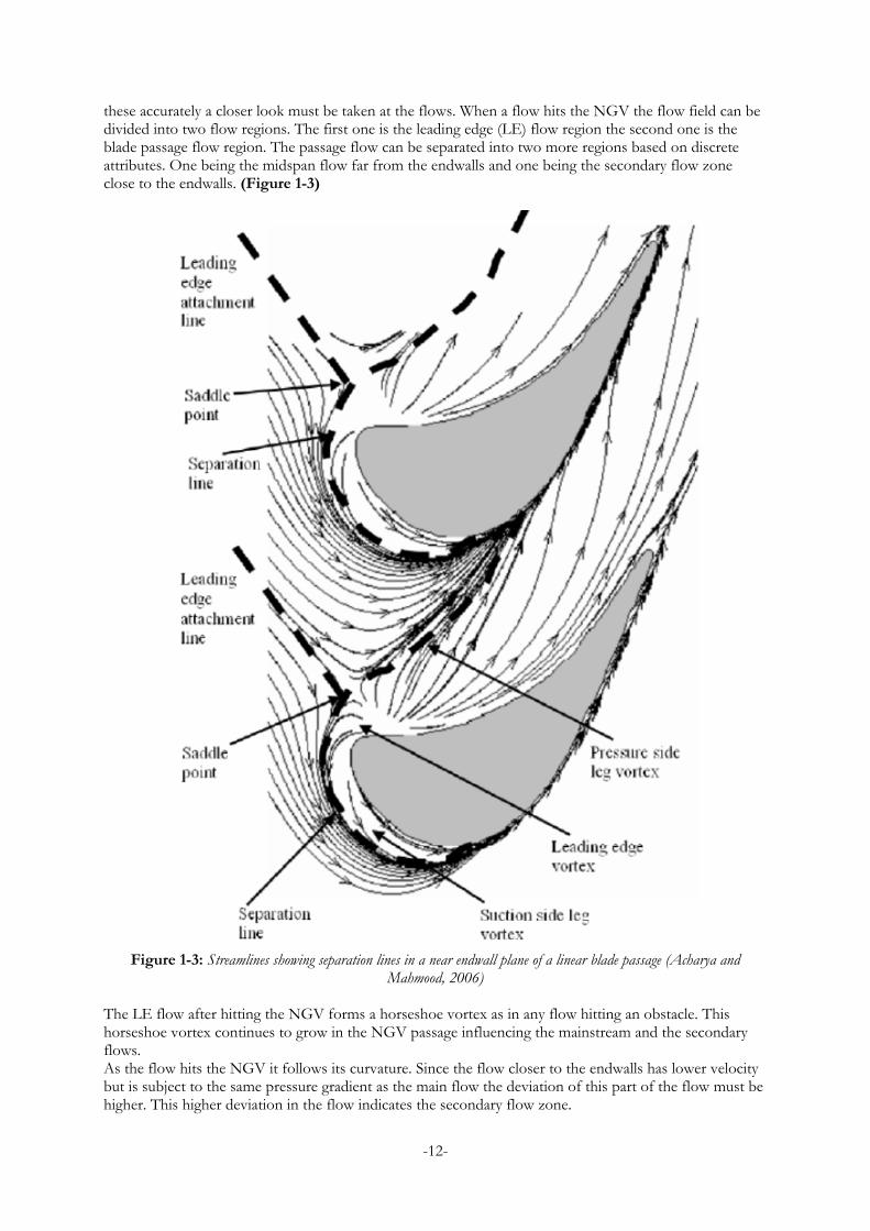
these accurately a closer look must be taken at the flows. When a flow hits the NGV the flow field can be divided into two flow regions. The first one is the leading edge (LE) flow region the second one is the blade passage flow region. The passage flow can be separated into two more regions based on discrete attributes. One being the midspan flow far from the endwalls and one being the secondary flow zone close to the endwalls. (Figure 1-3)

Figure 1-3: Streamlines showing separation lines in a near endwall plane of a linear blade passage (Acharya and

Mahmood, 2006)

The LE flow after hitting the NGV forms a horseshoe vortex as in any flow hitting an obstacle. This horseshoe vortex continues to grow in the NGV passage influencing the mainstream and the secondary flows. As the flow hits the NGV it follows its curvature. Since the flow closer to the endwalls has lower velocity but is subject to the same pressure gradient as the main flow the deviation of this part of the flow must be higher. This higher deviation in the flow indicates the secondary flow zone.

-13-

The passage flow is affected by both of afore mentioned and other flow phenomena. However the complete flow is much more complicated and consists of more parts such as crossflows from the pressure side to the suction side at the trailing edge, the complex passage vortex and counter rotating secondary vortexes behind the trailing edge (TE) (Saha, R. 2014) (Figure 1-4).

Figure 1-4: Passage and horseshoe vortexes (Model of Sharma and Butler 1987)

There have been numerous studies conducted on linear cascades with high exit velocities, but these experiments neglect the three dimensional pressure gradients which are present in real life machines. Turning nonuniform flows into linear cascades creates three-dimensional flows with the flow angle varying along the blade span. This phenomenon becomes even more important in annular machines where nonuniformity of the flow is a starting parameter (D. R. Glynn and H. Marsh 1980).

1.2 State-of-the-art Aerodynamic Losses Losses in general are indicating some kind of rise in entropy. This means that there is a part of the process which cannot be reversed, in other words it is lost as useful energy. Losses can be defined as the difference between the ideal and the actual energy at the end of the process (Saha, R. 2014).

The losses can come from various places in a flow. The ones coming from the mixing of the flow and the boundary layer viscosity are considered the largest sources. These losses can be the result of profile losses or mixing losses caused by friction either between the fluid and the NGV or within the fluid itself. Some studies state that the highest losses in passage flows arise from the boundary layers near the endwalls caused by the endwall vortexes and that they have large impact on the flow behaviour downstream. But it needs to be mentioned that not all the loss creating mechanisms are fully understood yet (Bartl, J. 2010).

In flow measurements like the present one it is common to use a loss coefficient which is a non-dimensional indicator of the losses. Of course the same loss coefficient cannot be used for the cooled and the uncooled cases. The one used for the uncooled case will be:

𝜁 = 1 −𝐴𝐴𝐴𝐴𝐴𝐴 𝑒𝑒𝑒𝐴 𝑘𝑒𝑘𝑒𝐴𝑒𝐴 𝑒𝑘𝑒𝑒𝑒𝑒 𝑜𝑜 𝐴ℎ𝑒 𝑜𝐴𝑜𝑓

𝐼𝐼𝑒𝑘𝐴𝑒𝑜𝐼𝑒𝐴 𝑘𝑒𝑘𝑒𝐴𝑒𝐴 𝑒𝑘𝑒𝑒𝑒𝑒 𝑜𝑜 𝐴ℎ𝑒 𝑚𝐴𝑒𝑘𝐼𝐴𝑒𝑒𝐴𝑚 𝑜𝐴𝑜𝑓

-14-

The loss coefficient of the cooled case needs to include the kinetic energy of the coolant flow. This will result in:

𝜁 = 1 −𝐴𝐴𝐴𝐴𝐴𝐴 𝑒𝑒𝑒𝐴 𝑘𝑒𝑘𝑒𝐴𝑒𝐴 𝑒𝑘𝑒𝑒𝑒𝑒 𝑜𝑜 𝐴ℎ𝑒 𝑜𝐴𝑜𝑓

𝐼𝐼𝑒𝑘𝐴𝑒𝑜𝐼𝑒𝐴 𝑘𝑒𝑘𝑒𝐴𝑒𝐴 𝑒𝑘𝑒𝑒𝑒𝑒 𝑜𝑜 𝑚𝐴𝑒𝑘𝐼𝐴𝑒𝑒𝐴𝑚 + 𝐼𝐼𝑒𝑘𝐴𝑒𝑜𝐼𝑒𝐴 𝑘𝑒𝑘𝑒𝐴𝑒𝐴 𝑒𝑘𝑒𝑒𝑒𝑒 𝑜𝑜 𝐴𝑜𝑜𝐴𝐴𝑘𝐴

In practice the efficiency of the cooled cascade is more a ratio of kinetic energies of the coolant and main flow mixture after the cascade and the energies represented in the main flow and the coolant flow before entering the cascade. This ratio can be expressed as:

𝜂 =0,5(𝑚1 + 𝑚𝑐)𝐴22

𝑚1ℎ1,𝑖𝑖𝑖 + 𝑚𝑐ℎ𝑐,𝑖𝑖𝑖

Where m1 is the main gas mass flow and mc is the coolant mass flow and h represents the enthalpies respectively. From this the loss of the cooled cascade can be put as:

𝜁 = 1 − 𝜂 = 1 − 𝜑21 + 𝑌

1 +𝑌ℎ𝑐,𝑖𝑖𝑖ℎ1,𝑖𝑖𝑖

Where η is the efficiency of the cooled vane, φ is the velocity coefficient and Y is the mass flux ratio between the coolant and the main gas mass flow known as the mass-flux ratio. The velocity coefficient is described as:

𝜑 =𝐴2𝐴2,𝑖𝑖𝑖

=𝑀2

𝑀2,𝑖𝑖𝑖�𝑇𝑚𝑖𝑚

𝑇1

Where M represents the Mach number and T the temperature and u2 stands for the mixed flow average velocity at the outlet while the iso index stands for the isentropic values for the same parameter. With the help of isentropic relations the following equations can be presented:

𝑀22

𝑀2,𝑖𝑖𝑖2 =

�1 − 𝐼2𝑖𝑠𝐼2

�𝜅−1𝜅

�1 − 𝐼2𝑖𝑠𝐼1

�𝜅−1𝜅

ℎ𝑐,𝑖𝑖𝑖

ℎ1,𝑖𝑖𝑖=

1 − �𝐼2𝑖𝑠𝐼𝑐�𝜅−1𝜅

1 − �𝐼2𝑖𝑠𝐼1�𝜅−1𝜅∗𝑇𝑐𝑇1

Since the losses and efficiencies in the experimental environment are dependent on several parameters which are hard to simulate usually they are expressed as quantified terms. These usually are pressures and temperatures. To be able to quantify them in to these terms some assumptions are needed.

• The flow is isothermal there is no temperature difference between the coolant and the main flow.

-15-

• The gas constant R and the specific heat capacity κ are the same for the coolant and the main flow.

• The mixing between the coolant and the main flow is perfect.

With the application of these assumptions the loss equation for a cooled vane can be presented as:

𝜁 = 1 −(1 + 𝑌)�1 − �𝐼2𝑖𝑠𝐼2

�𝜅−1𝜅 �

�1 − �𝐼2𝑖𝑠𝐼1�𝜅−1𝜅 � + 𝑌 �1 − �𝐼2𝑖𝑠𝐼𝑐

�𝜅−1𝜅 �

One can realize that by setting the mass flux ratio Y to 0 the uncooled loss coefficient can be reached. However it needs to be mentioned that in practice this not necessarily applies because the assumptions mentioned before (Saha, R. 2014). This loss is often called primary or enthalpy loss coefficient.

𝜁 =�𝐼2𝑖𝑠𝐼2

�𝜅−1𝜅 − �𝐼2𝑖𝑠𝐼1

�𝜅−1𝜅

1 − �𝐼2𝑖𝑠𝐼1�𝜅−1𝜅

In the past this loss bore then names endwall loss, profile loss and leakage loss, however these losses are separate and independent (Denton, 1993). The endwall loss is accountable for losses in the secondary flows in the boundary layers close to the endwalls. The profile losses are created in the boundary layers but far from the endwalls. The tip leakage is present over the tip of the blades and stators. The relative significance of these losses are dependent on the specific machine characteristics such as tip clearance and blade aspect ratio, but often each of these losses are accountable for around one third of the total aerodynamic loss (Denton, 1993). While causing efficiency drops on their own the interactions between these losses also cause losses. When the blade surfaces are increased for instance in low aspect ratio cascades the secondary losses show a significant increase (Saha, R. 2014).

The determination of the loss coefficient is dependent on a lot of parameters like the geometry which is influenced by the inlet angle, pitch to chord ratio, TE thickness etc. and flow parameters as the Reynolds number, compressibility etc.

The total loss coefficient will be the summation of all the loss coefficients which are standing for each individual loss. To get a precise value of these would require measurements in the real life machine. This of course is rarely possible due to the operating temperatures of gas turbines and the accessibility of these machines due to costs. There are some ways around this such as cold flow tests one of which is discussed in this study. Of course these are in need of scaling the conditions to obtain a flow with similar characteristics as the real flow would be. There are a few methods which are applied in this field. It can be a linear cascade, an annular cascade or like in this paper an annular sector cascade (ASC). The reasoning behind using this type of model is that like in a real 3D flow there are radial pressure gradients which can’t be modelled in linear cascades.

Investigating the flow behaviour at different exit Mach numbers in an ASC shows the following results. Increasing the Mach number in the subsonic region, while staying in the incompressible field, shows some distinct characteristics. The secondary flows will have smaller penetration depth into the mainstream flow making them remaining closer to the endwalls. The passage vortex decreases in size while the corner and counter vortex size increases. A contraction in the exit flow angle variation can be observed too. Changing the Mach number will come forward as pushing the ASC into off design conditions which will have effect

-16-

on the Reynolds number, the loading of the blades and many other parameters. Since the cascade is designed for one particular Mach number to obtain precise measurement data for each Mach number the cascade would need to be redesigned. In general it can be observed that the loss coefficient of the flow decreases with the higher Mach numbers until one reaches the shock region and the shock losses start to play part in the process (Saha, R. 2014).

1.3 Shockwave Losses and Boundary Layer Interaction With the increasing speed of aircrafts and velocities in turbines, reaching the sound barrier was unescapable. Reaching this limit means the introduction of shocks in the flow which of course translates into losses. In the past many theoretical and experimental researches were carried out on this topic. Even though there is a large amount of knowledge the phenomenon is still not fully understood, making it necessary to carry out further investigations like present study. In a flow without a boundary layer when it reaches the sonic velocity a shockwave is generated, reflected or met by a solid surface. The shockwave is a result of the flow decelerating because of an obstacle in its way. In this ideal flow the pressure would discontinuously increase. However in a real flow the fluid in the boundary layer has subsonic velocity therefore cannot go under irregular pressure change. As a result of this part of the pressure change is channelled upstream in the subsonic boundary layer. This generates a divergence in the streamlines which will cause compression waves in the supersonic part fluid (Bodony and Smith 1986).

In a study carried out by Perdichizzi in 1989 the Mach number was raised in a linear cascade from Mach 0.3 up to 1.55. This research found that in the subsonic region the secondary losses are nearly uniformly distributed in the top/bottom quarter of the span and decreasing towards the midspan because the high velocity of the passage vortex. Around the tip and the hub regions the losses are higher since the corner vortex fades and because of the sheer stresses at the endwalls. In the subsonic region Mach number rising causes the losses to decrease because the expansion of the flow is smaller than at lower velocities, causing the mixing and secondary losses to contract. This is followed by the reduction in the flow deviation. Reaching the supersonic region the loss cores are moving close to the endwalls while increasing in magnitude while in the passage closer to the midspan region they tend to decrease even more (Figure 1-5). This is due to the shock losses occurring mostly in the boundary layers while the importance of the passage vortex is decreasing. When choking is reached, the loss core remains in the same position. With higher Mach numbers, the flow deviation angle decreases both in over and underturning (Figure 1-6). This occurs because the primary velocities raise more in magnitude than the secondary ones and become more dominant in the flow. At high velocities a small overturning can be observed close to the endwalls which is imputable to the increased role of the corner vortex

-17-

Figure 1-5 Spanwise loss distribution at different Mach numbers (Perdichizzi 1989)

-18-

Figure 1-6 Spanwise exit flow angle distribution at different Mach numbers (Perdichizzi 1989)

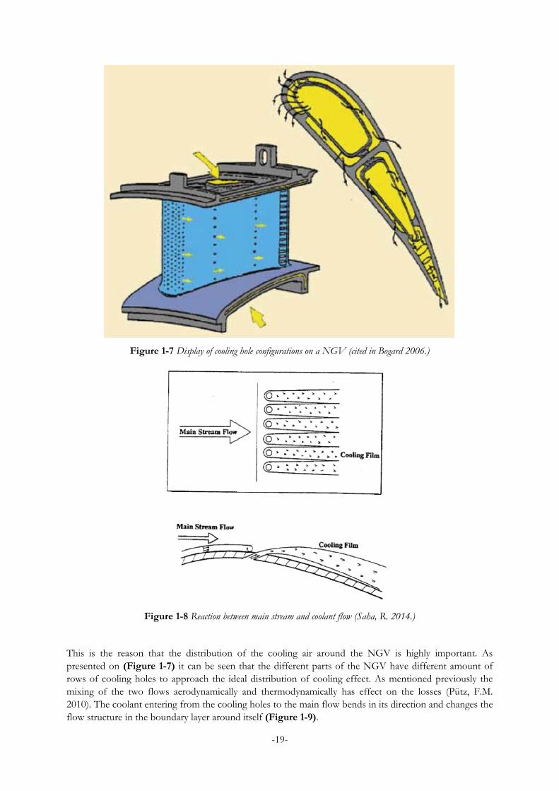
1.4 State-of-the-art in External Cooling In gas turbines to reach higher efficiencies TET is raised well over the melting point of the NGV material. To prevent the blades from melting external cooling is used (Figure 1-7). This means that air from the compressor is bypassed the combustion chamber and pushed through the cooling holes of the blades creating an air film to protect the blades not only around the hole but even downstream from it as presented in (Figure 1-8). Taking air away from the process can highly decrease the overall efficiency depending on the amount which in some cases can go up to 20-30% unless the TET is raised high enough to balance out these losses (Saha, R. 2014). Since the air is not heated in the combustion chamber when entering through the cooling holes it causes a thermodynamic loss. To reduce this loss as much as possible the amount of cooling air bypassing the combustion chamber is needed to be kept at the sufficient minimum.

-19-

Figure 1-7 Display of cooling hole configurations on a NGV (cited in Bogard 2006.)

Figure 1-8 Reaction between main stream and coolant flow (Saha, R. 2014.)

This is the reason that the distribution of the cooling air around the NGV is highly important. As presented on (Figure 1-7) it can be seen that the different parts of the NGV have different amount of rows of cooling holes to approach the ideal distribution of cooling effect. As mentioned previously the mixing of the two flows aerodynamically and thermodynamically has effect on the losses (Pütz, F.M. 2010). The coolant entering from the cooling holes to the main flow bends in its direction and changes the flow structure in the boundary layer around itself (Figure 1-9).

-20-

Figure 1-9: Jet to the main flow from a single cooling hole (Pütz, F.M. 2010.)

As a result of the bending the mainstream flow increases its velocity around and above the jet and decreases it up and downstream of it. This results in a horseshoe vortex around the jet as it would be around a cylinder in any other flow. The mixing process is a complex 3D phenomenon in the boundary layer which depends on several parameters such as the inlet velocity of the cooling air the coolant to mainstream mass flow ratio and the temperature difference between the coolant and the main stream flow which affects the density ratios. To ensure a good mixing between the coolant and the mainstream the right amount of coolant has to be injected with the right angle and the right velocity. To quantify these terms the following parameters have been introduced. The mass flux ratio (Y), the blowing ratio (BR), the momentum flux ratio (MR) and the density ratio (DR).

𝑌 =𝑚𝑐

𝑚𝑚

𝐵𝐵 =𝜌𝑐𝐴𝑐𝜌𝑚𝐴𝑚

𝑀𝐵 =𝜌𝑐𝐴𝑐2

𝜌𝑚𝐴𝑚2

𝐷𝐵 =𝜌𝑐𝜌𝑚

The blowing ratio can be defined various ways. It is either described with the parameters of the flow field upstream or with the local parameters at the different cooling row arrangements. The blowing ratio will provide information about the velocity ratios of the different flows by representing the coolant mass flux injected into the mainstream flow. The momentum-flux highly affects the flow field dynamics through the jets penetration into the mainstream flow. Depending on the magnitude of the momentum flux the coolant distribution can differ. The coolant can attach to the surface, detach and then reattach or lift off completely from it (Figure 1-10).

-21-

Figure 1-10: Boundary layer pattern for different momentum-flux ratios (Saha, R. 2014.)

The most common places to put the external cooling holes are the leading edge, pressure and suction side trailing edge and the endwalls. The most bypass air is usually used at the LE cooling since these parts of the turbine vanes are experiencing the highest thermal loads. This means the installation of numerous cooling rows often referred as shower head (SH) cooling. Other than preventing the LE from melting the SH cooling has a considerable effect on the flow development. On the contrary of its importance the efficiency of the SH cooling is very poor. This is a result of many factors and effects of the complex flow around the LE. These include the stagnation line, the really thin or non-existent boundary layer the high pressure gradients, multiple interactions between the coolant and the main flow and high turbulence levels partly caused by the coolant injection facing the main flow. Since the stagnation line in an actual turbine cannot be properly located the practice is to install an extra cooling row on each side as compensation. However the proper calculations are highly important as they determine how much coolant will flow around the pressure side (PS) or the suction side (SS).

Experiments carried out at low Mach numbers on linear fully cooled cascades (Barigozzi et al. 2001) showed that the coolant injection on the PS will not affect the boundary layer in a turbulent way letting it being laminar up until the TE. As a result of this the PS losses mainly are mixing losses. On the other hand the coolant entering on the SS has a large impact on the boundary layer. It enlarges the boundary layer and makes it more turbulent. This results in a loss ratio of 2/3 on the SS and 1/3 on the PS. Other studies (Jackson et al. 2000) point out that the mixing losses are significantly higher than the ones caused by the shock waves at the TE. Many studies on many different setups were carried out on TE cooling. The combined results suggest that a coolant injection lower than 5% helps to reduce the mixing losses due to the elevated base pressure at the TE, however the coolant flow can result in loss increasing up to 80% (Aminossadati and Mee 2013). Although it needs to be mentioned, that these studies were carried out on different types of configurations and experimental setups. In conclusion of the external cooling applications it needs to be said that any kind of cooling has a negative effect on the cycle efficiency so from that point of view the coolant mass flow needs to be kept at the possible minimum.

1.5 Research motivation First and foremost after going through the related literature it can be seen that most of the studies are conducted on linear cascades. It is a widely accepted fact that the secondary flow structures look different in a linear than an annular sector cascade. Same goes to the 2D models compared to the 3D ones. This

-22-

makes ASC experiments necessary in order to get the radial pressure gradients right. Other reasoning behind the ASC studies is that ASCs resemble real life machines much more than their linear counterparts. Secondly most of the past experiments were done in subsonic environment. Since todays trend is to push the turbines into tran and supersonic regions experiments with exit velocities from Mach 0.95 to 1.2 have to be performed. As mentioned before it is difficult to make models of such complicated and compound flows of an externally cooled NGV in a CFD environment. This makes the physical experiments necessary in order to make further improvements of the turbine efficiency possible and validate the numerical tools. Because of this contradiction in the literature it makes it important to run present experiment.

In the related literature there is no straight answer to the question, to which extent is external cooling increasing cycle efficiency? The application of external cooling allows reaching higher TET which allows higher Carnot efficiency, but the more air is bypassed the combustion the less energy is put into the cycle and the bypass air experiencing some more mixing and pressure losses. Another reason behind this is that it is really rare for experiments use the same equipment. As mentioned earlier, there is no definite answer regarding the secondary flow development, mostly because it appears as high momentum flow injection in a low momentum region. Present study is important because it will help gather data on fully cooled 3D ASC NGVs and thus help future development and improvements. Also the gathered data might help developing more accurate calibration and loss coefficient calculating methods.

1.6 Objectives The main objective of this thesis is to quantify the losses in the NGV of a high pressure turbine (HPT) stage and help to give a more detailed understanding of the efficiency behaviour in the tran- and supersonic regions in the cooled and the uncooled case. The efficiency is highly affected by the secondary flow pattern and the coolant flow development. As in a usual case the optimum efficiency is achieved when the minimal amount of coolant flow is found which fulfils the structural and thermal requirements while keeping the aerodynamic losses to a minimum.

The main objectives of this thesis are the following:

• Run in-house calibrations at low Mach numbers to justify the tran- and supersonic calibration of the measurement probe provided by the manufacturer.

• Determine the aerodynamic performance of the high exit velocities on the flow around the middle NGV of the ASC, mainly the losses and exit flow angle deviation.

• Experimentally explore the aerodynamics of the same flow when full film-cooling is applied. • Find and interpret the differences of the cooled and uncooled flow structures. • From the experimentally obtained data give a statement on how big influence the Mach number

raising and the application of film-cooling affects the efficiency in the cases mentioned before.

1.7 Methodology To reach the goals set among the objectives an action plan was needed. To carry out a useful and productive work the following points were set to meet the scientific standards of KTH.

1.7.1 Literature study

To understand the work done in this field and the state of the art at the beginning of this research extensive literature study had to be done. In this part it is essential to get a preconception of what results the experiment might produce. There are several papers written about the same test rig regarding experiments close to this present one. Most of these papers investigate the differences between the different external cooling methods. All these papers let the reader get some kind of idea about the flow

-23-

field around the NGVs. However it is important to study papers written on flow field development to get a more accurate picture. After studying the research papers an idea of what outcomes can be expected started to materialize.

1.7.2 Probe calibration

The probe used for these measurements is a 5 hole L shaped probe manufactured by the Aeroprobe Corporation. The tip is 1.6 mm in diameter and 40 mm in length. Before beginning the measurements it is essential that the probe used for the experiments is calibrated to the operating conditions. The probe is supported by a calibration sheet from the factory but to be totally convinced about the applicability of the factory calibration coefficients comparative calibration has to be done internally. Since the most data are presented at Mach 0.8 this value was chosen to be the base for the comparison. After running the internal calibration the calibration coefficients need to be calculated both for the factory and the KTH cases. When all the calibration coefficients are calculated, the factory and KTH cases must be compared to ensure that the probe is measuring inside the given limits. When made sure that the two cases overlap, calibration coefficients for the higher Mach numbers from the factory calibration sheets can be calculated. Other than the coefficients the pressure response time of the probe has to be tested too.

1.7.3 Assemble the test rig

For the first measurement which is the uncooled case the cooling holes of the NGVs are blocked to prevent cross communication and thus getting false values in the measurements. To ensure this a special type of beeswax was plugged into the cooling holes. After the beeswax is applied the assembly can begin. Following the assembly manual the test rig components has to be assembled. For the pressure measurements a PSI setup has to be composed. This setup needs to contain which pressure channel will measure which pressure. The pressure tubes had to be examined for leakages and damages. The next step is to create a measurement path or grid for the probe. This needs to contain the path the probe will follow, the vertical and horizontal distance between the measurement points, the time it needs to wait between taking measurements and the speed which with the probe can move between the points.

1.7.4 Run periodicity trials

After the rig is assembled periodicity trails with the probe at 50% span position were performed in order to see if continuous readings can be obtained and to find leakages and any kind of unseen trouble with the rig assembly. If any leakage or problem shows up solution must be found and applied before the measurements can take place. When ensured that no leakages or troubles will affect the measurements, pressure readings at 50% were taken. If needed the “re-zeroing” of the equipment can be done.

1.7.5 Uncooled Case Measurements

Run the uncooled version of the measurements. After running the measurements the data needs to be assessed and evaluated.

1.7.6 Cooled Case Measurements

To begin the cooled version of the experiment the rig needs to be dissembled and the beeswax needs to be removed from some of the cooling holes. When done, the rig is to be assembled again. Before running a leakage test is performed. If necessary the “re-zeroing” of the equipment can be also done. After that the cooled measurements can be run, data collected and evaluated.

1.7.7 Data evaluation

After all data collected the evaluation process can be done. From the evaluated data conclusions for the individual cases and for the comparison can be drawn. With the help of the results the hypothesis can be

-24-

supported or refuted. As a last step a statement on advantages and disadvantages on increasing the Mach number in the ASC shall be given.

1.8 Research Limitations The first big limitation of present experiment is the cold flow itself. In a real engine the temperatures are around 1400-1700 °C at the HPT stage (Birch, N. T., 2000.). Another problem is that in a real machine it would be flue gas instead of air flowing through the NGVs. As a result only the Mach number of the flow can be matched, the Reynolds number not. The intensity of the turbulence is noticeably higher in a real machine then in the ASC used in present experiment. This means that the profile losses and the secondary losses will not be the same as they would be in a real life engine. As it name indicates the cooling flow presents another limit as in present investigation the coolant and the mainstream flow are nearly the same temperature as in reality there usually is a difference of one magnitude. Hence these limitations the results of this experiment are believed to help the industry to validate their simulation codes and results for the test rig conditions.

-25-

2 Experimental approach

2.1 NGV Geometry and Cascade Arrangement For this experiment NGVs with the same geometrical features as ones in a real gas turbine were used. This meant cooling holes in the same places and the same profiles as one can expect from a real NGV. The design parameters of these vanes such as pitch/chord ratio or inlet flow angle shall be identical. These parameters can be found in Table 2-1 below.

Table 2-1: Geometric parameters of NGV

Design Parameter Value Unit True chord at midspan (c) 0,1292 m Axial chord at midspan (cax) 0,0665 m Axial chord at hub radius 0,0625 m Pitch-to-chord (s/c) ratio at midspan 0,826 Hub radius at exit 0,6153 m Tip-to-hub ratio at exit 1,097 Aspect ratio based on TE vane height 0,463 Inlet metal angle 90 deg Reference effective exit angle 16,05 deg Stagger angle (x) 33,3 deg LE radius 0,0138 m TE radius 0,0014 m Uncovered turning angle 19 deg

Figure 2-1: Scheme of profile geometric parameters (Saha, R. 2014.)

As mentioned earlier these vanes have cooling holes included. This is shown on Figure 2-2 from various angles.

-26-

Figure 2-2 Cooling holes on the NGV (Saha, R. 2014.)

These cooling holes can be divided into four different regions as shower head (SH), suction side (SS) pressure side (PS) and trailing edge (TE). These regions can be further divided into rows. SH cooling has 6 rows, suctions side is divided into SS1 and SS2 sub-regions both with 2 rows each PS has one row and so does TE cooling. The cooling holes which are located on the platform of the NGV were blocked for all experiments. The number of holes per row the exit angles and the location of the holes are presented in Table 2-2. The cooling exit angle is measured from the tangent of the cooling exit point. A schematic picture of these is presented in Figure 2-3.

Table 2-2 Cooling geometric information

Row x/cax Angle of holes as midspan, θ [°] No. of holes

SH1 3.3% 56.7 26 SH2 0.89% 74.6 25 SH3 0% 80.4 26 SH4 0.77% 66.9 26 SH5 3.4% 53 25 SH6 9.1% 46.3 11 PS1 77% 38.2 23 SS1 (2rows) 19%, 23% 50.9, 59.3 24, 23 SS2 (2rows) 50%, 52% 42.3, 38.9 23, 22 TE 100%

-27-

Figure 2-3 Cooling hole locations on the NGV (Saha, R. 2014.)

Although the ASC has three NGVs it is enough to only investigate the area around the middle vane (Saha R, Fridh J. 2015). The shape of the cooling holes is cylindrical with a diameter of 0.0007 m. For the uncooled case the cooling holes were sealed with special adhesive beeswax.

2.2 Description of the Rig, Cascade Arrangement and Measuring Equipment

The ASC test rig is designed to be able to test different types of arrangements in order to improve gas turbine efficiency. The rig is located in the Wind Tunnel Laboratory of the Division of Heat and Power Technology at KTH Royal Institute of Technology Stockholm Sweden. A schematic representation of the rig and the supplying facilities is pictured on Figure 2-4.

Figure 2-4 Schematic picture of the air supply system and the test rig (Saha, R. 2014.)

-28-

A twin screw compressor powered by a 1 MW electric motor is responsible for supplying the air. After leaving the compressor the air has an absolute pressure of 4 bars and a cooling system reduces the air temperature to a stable 313 K. The mass flow can be controlled by two bypass valves and two inlet valves and with these conditions can go up to 4.7 kg/s. At the exhaust of the system is another controllable valve and an exhaust fan to make the operation point setting easier.

(1) Inflow, (2) Settling chamber, (3) First radial contraction, (4) Turbulence grid, (5) Second

radial contraction, (6) Test sector with NGVs, and (7) Outflow Figure 2-5 ASC Arrangement (Saha, R. 2014.)

Figure 2-5 shows the route of the airflow throughout the rig. The air first enters into the settling chamber where it passes through the turbulence grid which has a honeycomb five mesh to make the flow homogenous. After the settling chamber the cross section goes from circular to an annular shape in a contraction. In the annular section there is a changeable turbulence grid, which is responsible for producing different inlet profiles. In present study a parallel bar turbulence grid was used. After the turbulence grid the flow hits the ASC which has an opening of 36° and consist of three NGVs and two side walls. The aerofoils are NGV-1, NGV 0 and NGV+1 as shown on Figure 2-6.

Figure 2-6 ASC radial view (Saha, R. 2014.)

-29-

To gather measurement data downstream of the ASC a fully automatized traverse mechanism (Appendix B) was used. All the measurement points up or downstream are presented in Figure 2-7. The locations of these measurement points are presented in Table 2-3.

Figure 2-7 Axial cross section of ASC (Saha, R. 2014.)

Table 2-3 Position of measurement points

Measurement points Location (reference at LE hub) Notes

Turbulence grid -264% cax,hub 1.5% turbulence intensity (Pütz 2010)

1 -55.7% cax,hub Upstream traverse location 2 107.7% cax,hub Downstream traverse location 3 136.5% cax,hub Hub pressure taps

The inlet measuring plane located at -55.7% cax,hub was not used in present experiment. The total pressure upstream was measured by a three hole cobra probe located in the settling chamber marked with (2) on Figure 2-5. This probe was calibrated in the in-house calibrating wind tunnel. The downstream measurements were obtained at position 2, 107.7% cax,hub where the measurement probe was located and at position 3, 136.5% cax,hub where the 31 static pressure taps on the hub are. The downstream probe at position 2 is a 5 hole L shaped probe with 1.6 mm tip diameter and 40 mm tip length presented on Figure 2-8 and Figure 2-9.

-30-

Figure 2-8 Aeroprobe (courtesy of Aeroprobe Corporation)

Figure 2-9 Aeroprobe front view (courtesy of Aeroprobe Corporation)

-31-

For the cooled case the cooling air was delivered from a 5 m3 vessel pressurized to 40 bar and regulated before entering into the mass flow controllers which are responsible for measuring and distributing the coolant to each vane. For both measurements the L probe was mounted to the traverse mechanism and traversing the area behind the NGV 0. This meant 1443 measurement points, 39 tangential and 37 radial covering 6%-96% of the span. The measurement points were distributed in order to be denser around the areas where the wakes and the secondary vortexes are expected. This is shown on Figure 2-10.

Figure 2-10 Grid of measurement points (Saha, R. 2014.)

Unlike the convention Figure 2-10 looks at the ASC from the downstream. This means the left side of NGV 0 is the SS and the right side is the PS. The horizontal axis shows the normalised pitch-wise location while the vertical presents the normalised span.

2.3 Calibration of the Measurement Probe Calibration of the measurement probe is necessary to ensure precise data from the measurements. The probe used for this experiment is a 5 hole, L shaped probe manufactured by the Aeroprobe Corporation. The probe came with its own calibration sheets from Mach 0.8 up to 1.3. To justify the factory data an in-house calibration was carried out at Mach 0.8 and compared to the corresponding factory calibration sheet. The calibration was done in the Wind Tunnel Laboratory in a semi open calibration rig. The calibration consists of two parts.

The first part is to test the response time of the probe in order to know how much time is needed for the probe to stay in place before taking a measurement. This is done by putting an inflated balloon on the probe tip covering all pressure taps and when the readings are stabilised the balloon is popped and the settling time of the pressures is logged. The response time for the probe used was 6 seconds.

-32-

The second one is calibration for different tangential (yaw) and radial (pitch) angles in a flow with known and constant velocity. In this part, pressures are measured through the 5 pressure taps on the probe tip and logged with the corresponding pitch and yaw angles. As a second step from the raw pressure data dimensionless calibration coefficients are calculated.

For this calibration setup the probe and wind tunnel pressures were logged by a PSI9116 TM system while the atmospheric pressure was measured by a Solartro TM barometer. The logging of the data is done by, a KTH developed software LabView TM. The probe is calibrated between -20° to +20° both for pitch and yaw with the pitch angles raging (-20, -18, -16, -13, -10, -8, -6, -4, -2, -1, 0, 1, 2, 4, 6, 8, 10, 13, 16, 18, 20) and the yaw angles being (-20, -18, -16, -14, -12, -10, -8, -6, -4, -2, -1, 0, 1, 2, 4, 6, 8, 10, 12, 14, 16, 18, 20). In order to obtain a stable velocity flow a calibration nozzle is inserted into the calibration rig which is shown on Figure 2-11. The probe tip is set to a stable point using an optical laser system. This ensures the tip remaining in the same place while traversing through different pitch and yaw angles for the calibration.

Figure 2-11 Calibration nozzle (Fridh J. 2010)

From the raw pressure data dimensionless calibration coefficients are calculated. The indexes of the pressures are corresponding to Figure 2-9 with pt indicating the total pressure measured in the settling chamber and pst the static pressure which is measured on the sidewall in line with the probe tip. The setting of the Mach number for the flow is calculated using the following equation:

𝑀 = ���𝐼𝑠𝐼𝑖𝑠

�𝜅−1𝜅� ∗

2𝜅 − 1

The coefficients are:

Total pressure coefficient 𝐾1 = 𝑝0−𝑝1𝑝1−

(𝑝2+𝑝3+𝑝4+𝑝5)4

-33-

Static pressure coefficient 𝐾2 = 𝑝0−𝑝𝑠𝑠𝑝1−

(𝑝2+𝑝3+𝑝4+𝑝5)4

Yaw coefficient 𝐾3 = 𝑝2−𝑝3𝑝1−

(𝑝2+𝑝3+𝑝4+𝑝5)4

Pitch coefficient 𝐾4 = 𝑝4−𝑝5𝑝1−

(𝑝2+𝑝3+𝑝4+𝑝5)4

From the gathered pressure data the coefficients were calculated and plotted as surface curves using a MATLAB TM code as shown on Figure 2-12 for Mach 0.8. These coefficients then were compared to those supplied by the industry. The result of the comparison showed that the coefficients were almost identical and to some extent increase reliability and applicability of the factory coefficients for the higher Mach numbers. This comparison is visualised on Figures 2-13 at the pitch angle of 0° with the pressures normalised with the total pressure values.

Figure 2-12 Calibration coefficient plots for Mach 0.8

It is important to point out that the shape of the graph indicators is the important feature of the curves not the pressure point indexes, since in the Aeroprobe calibration the probe is rotated 90° compared to the KTH calibration. It can be seen that the curves corresponding pressure taps are in line with each other. The “f” index and the red marker stands for the factory data. For further comparison in Figure 2-14 and Figure 2-15 the K1 calibration coefficient is presented for the KTH and for the Aeroprobe cases. As it can be seen, despite a slight difference at the corners of the curved surfaces the surfaces are nearly identical. However the Aeroprobe Corporation uses the cone angle and rolling angle approach of setting the calibration points while KTH the standard pitch-yaw approach so some points had to be interpolated in the provided factory data to acquire values at the same points. This might be the reason behind the slight offset between the two graphs.

-34-

Figure 2-13 Normalised pressure comparison at pitch 0° at Mach 0.8

K1 Coefficient for KTH at Mach 0.8

0,6

0,65

0,7

0,75

0,8

0,85

0,9

0,95

1

1,05

-30 -20 -10 0 10 20 30

pi/p

t

Yaw

Pitch 0°

p1/ptot

p2/ptot

p3/ptot

p4/ptot

p5/ptot

p1f/ptot

p2f/ptot

p3f/ptot

p4f/ptot

p5f/ptot

-20

-6

2

16

-0,050

0,050,1

0,15

0,2

0,25

0,3

0,35

0,4

0,45

-20 -16 -12 -8 -4 -1 1 4 8 12 16 20

Pitch

K1

Yaw

Total pressure coefficient KTH

0,4-0,45

0,35-0,4

0,3-0,35

0,25-0,3

0,2-0,25

0,15-0,2

0,1-0,15

0,05-0,1

0-0,05

-0,05-0

-35-

K1 Coefficient for Aeroprobe at Mach 0.8

-20

-6

2

16

-0,050

0,05

0,1

0,15

0,2

0,25

0,3

0,35

0,4

0,45

-20 -16 -12 -8 -4 -1 1 4 8 12 16 20

Pitch

K1

Yaw

Total pressure coefficient Aeroprobe

0,4-0,45

0,35-0,4

0,3-0,35

0,25-0,3

0,2-0,25

0,15-0,2

0,1-0,15

0,05-0,1

0-0,05

-0,05-0

-36-

3 Periodicity Trials

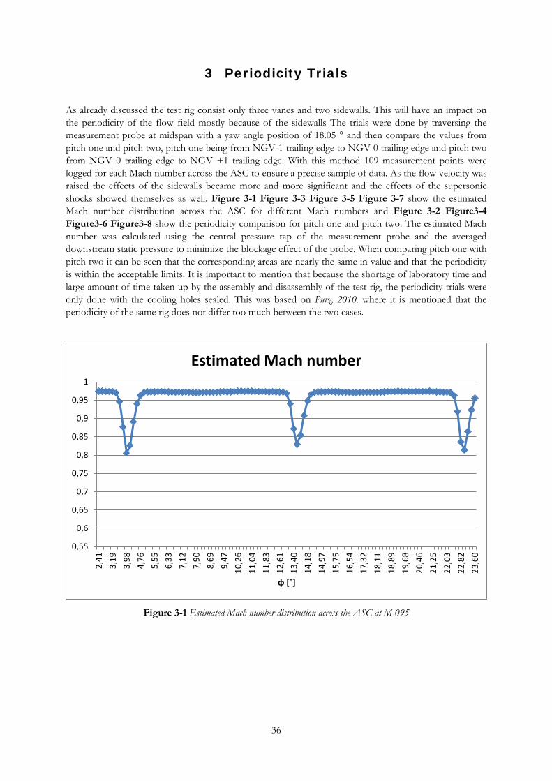
As already discussed the test rig consist only three vanes and two sidewalls. This will have an impact on the periodicity of the flow field mostly because of the sidewalls The trials were done by traversing the measurement probe at midspan with a yaw angle position of 18.05 ° and then compare the values from pitch one and pitch two, pitch one being from NGV-1 trailing edge to NGV 0 trailing edge and pitch two from NGV 0 trailing edge to NGV +1 trailing edge. With this method 109 measurement points were logged for each Mach number across the ASC to ensure a precise sample of data. As the flow velocity was raised the effects of the sidewalls became more and more significant and the effects of the supersonic shocks showed themselves as well. Figure 3-1 Figure 3-3 Figure 3-5 Figure 3-7 show the estimated Mach number distribution across the ASC for different Mach numbers and Figure 3-2 Figure3-4 Figure3-6 Figure3-8 show the periodicity comparison for pitch one and pitch two. The estimated Mach number was calculated using the central pressure tap of the measurement probe and the averaged downstream static pressure to minimize the blockage effect of the probe. When comparing pitch one with pitch two it can be seen that the corresponding areas are nearly the same in value and that the periodicity is within the acceptable limits. It is important to mention that because the shortage of laboratory time and large amount of time taken up by the assembly and disassembly of the test rig, the periodicity trials were only done with the cooling holes sealed. This was based on Pütz, 2010. where it is mentioned that the periodicity of the same rig does not differ too much between the two cases.

Figure 3-1 Estimated Mach number distribution across the ASC at M 095

0,55

0,6

0,65

0,7

0,75

0,8

0,85

0,9

0,95

1

2,41

3,19

3,98

4,76

5,55

6,33

7,12

7,90

8,69

9,47

10,2

611

,04

11,8

312

,61

13,4

014

,18

14,9

715

,75

16,5

417

,32

18,1

118

,89

19,6

820

,46

21,2

522

,03

22,8

223

,60

φ [°]

Estimated Mach number

-37-

Figure 3-2 Estimated Mach number periodicity at M 095

Figure 3-3 Estimated Mach number distribution across the ASC at M 1.05

0,75

0,8

0,85

0,9

0,95

12,

06,

110

,214

,318

,422

,426

,530

,634

,738

,842

,946

,951

,055

,159

,263

,367

,371

,475

,579

,683

,787

,891

,895

,910

0,0

Pitch [%]

Estimated Mach number periodicity

Pitch one

Pitch two

0,55

0,65

0,75

0,85

0,95

1,05

1,15

2,41

3,19

3,98

4,76

5,55

6,33

7,12

7,90

8,69

9,47

10,2

611

,04

11,8

312

,61

13,4

014

,18

14,9

715

,75

16,5

417

,32

18,1

118

,89

19,6

820

,46

21,2

522

,03

22,8

223

,60

φ [°]

Estimated Mach number

-38-

Figure 3-4 Estimated Mach number periodicity at M 1.05

Figure 3-5 Estimated Mach number distribution across the ASC at M 1.15

0,65

0,7

0,75

0,8

0,85

0,9

0,95

1

1,05

1,1

1,15

2,1

6,4

10,6

14,9

19,1

23,4

27,7

31,9

36,2

40,4

44,7

48,9

53,2

57,4

61,7

66,0

70,2

74,5

78,7

83,0

87,2

91,5

95,7

Pitch [%]

Pitch one

Pitch two

0,55

0,65

0,75

0,85

0,95

1,05

1,15

1,25

2,41

3,19

3,98

4,76

5,55

6,33

7,12

7,90

8,69

9,47

10,2

611

,04

11,8

312

,61

13,4

014

,18

14,9

715

,75

16,5

417

,32

18,1

118

,89

19,6

820

,46

21,2

522

,03

22,8

223

,60

φ [°]

Estimated Mach number

-39-

Figure 3-6 Estimated Mach number periodicity at M 1.15

Figure 3-7 Estimated Mach number distribution across the ASC at M 1.20

0,75

0,8

0,85

0,9

0,95

1

1,05

1,1

1,15

1,2

2,2

6,7

11,1

15,6

20,0

24,4

28,9

33,3

37,8

42,2

46,7

51,1

55,6

60,0

64,4

68,9

73,3

77,8

82,2

86,7

91,1

95,6

100,

0

Pitch [%]

Pitch one

Pitch two

0,55

0,65

0,75

0,85

0,95

1,05

1,15

1,25

2,41

3,19

3,98

4,76

5,55

6,33

7,12

7,90

8,69

9,47

10,2

611

,04

11,8

312

,61

13,4

014

,18

14,9

715

,75

16,5

417

,32

18,1

118

,89

19,6

820

,46

21,2

522

,03

22,8

223

,60

φ [°]

Estimated Mach number

-40-

Figure 3-8 Estimated Mach number periodicity at M 1.20

0,74

0,79

0,84

0,89

0,94

0,99

1,04

1,09

1,14

1,19

1,24

2,1

6,4

10,6

14,9

19,1

23,4

27,7

31,9

36,2

40,4

44,7

48,9

53,2

57,4

61,7

66,0

70,2

74,5

78,7

83,0

87,2

91,5

95,7

100,

0

Pitch [%]

Pitch one

Pitch two

-41-

4 Uncooled Measurements

To understand the effects of the external cooling on the main flow the secondary flows and the aerodynamic losses uncooled measurements were performed to see what losses already exist when the external cooling is added to the equation. Since the flow around the NGVs is identical (Saha et al. 2014) investigations only around NGV 0 were conducted. The temperature of the mainstream flow was set to 313 K. Since the HPT lab only has a cold measurement rig air is used as working fluid. This means that not all the conditions of a real engine can be simulated. The Reynolds number cannot be matched hence the temperature of the flow but the Mach numbers can be.

The first measurement was done at Mach 0.95. This measurement supported the expected results as mentioned in Part 1.3. The pressure distribution Figure 4-1 shows mostly uniform pressures in the vane passage while two loss cores can be observed in the tip and the hub region around the TE while boundary layer remains thin around the vane surface. Looking at the mass averaged loss coefficient Figure 4-2 and the area averaged exit flow angle deviation Figure 4-3 one can see the connection between the loss cores and low pressure regions at the tip and the hub. The Mach number distribution across the vane also shows the expected smooth distribution with the nominal value at the middle of the passage decreasing towards the endwalls as shown on Figure 4-4.

Figure 4-1 Total pressure distribution at Mach 0.95 uncooled case

-42-

Figure 4-2 Mass averaged kinetic energy loss Mach 0.95 uncooled case

Figure 4-3 Area averaged exit flow angle Mach 0.95 uncooled case

-43-

Figure 4-4 Mach number distribution at Mach 0.95 uncooled case

Getting on the other side of the transonic region at Mach 1.05, the boundary layer thickness increases as, the shocks start to arrive. The loss cores move closer to the tip and the hub region respectively Figure 4-5. The loss core in the hub region starts to expand more which trend will continue with the increased exit flow velocities. Despite being above Mach 1 the pressure distribution does not show any irregularities and is rather smooth across NGV 0. The small loss core in the top right corner of Figure 4-5 is coming from a glitch in the evaluating routine which could not be fixed before the writing of this paper.

-44-

Figure 4-5 Total pressure distribution at Mach 1.05 uncooled case

As the velocity increases there is a general raise in the exit flow angle Figure 4-7. This is due to the passage vortex becoming less relevant and the suction side of the horseshoe vortex more dominant.

-45-

Figure 4-7 Area averaged exit flow angle Mach 1.05 uncooled case

Reaching into the supersonic region at Mach 1.15 the effects of shocks are clearly visible on the pressure and boundary layer shown on Figure 4-9. The exit flow angle deviation continues to increase with the higher velocities but following the same distribution as before Figure 4-11. The Mach number distribution is much more hectic then before Figure 4-12. The borders of the boundary layer are much more clearly visible due to the effects of the shocks.

-46-

Figure 4-11 Area averaged exit flow angle Mach 1.15 uncooled case

Figure 4-12 Mach number distribution at Mach 1.15 uncooled case

-47-

At Mach 1.2 the effects of the shock losses can also be seen in the passage region. The low pressure regions at the tip and the hub expanded even more Figure 13. The boundary layer got thicker and the shifting process to the suction side is more significant than in the previous cases.

Figure 4-13 Total pressure distribution at Mach 1.20 uncooled case

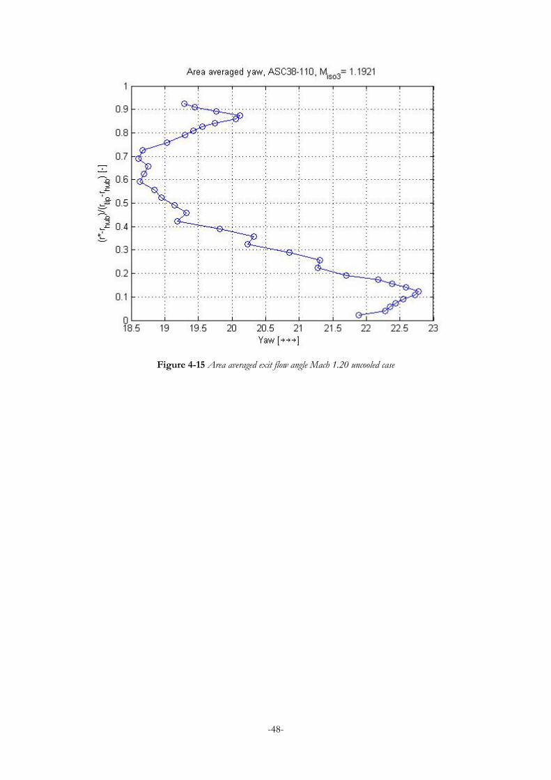
-48-

Figure 4-15 Area averaged exit flow angle Mach 1.20 uncooled case

-49-

5 External Cooling Measurements

As discussed in detail in the earlier chapters external cooling is introduced in turbines in order to TET can be raised above the melting point of the blade material. The application of cooling of course does not only alter the heat transfer but the flow characteristics too. Since this study is conducted in a cold test facility the focus is only on the altercation in flow characteristics. The most common method is to use the blowing ratio (BR) as mentioned in Chapter 1.4. Since air was used as cooling fluid the density ratio was considered one hence the small temperature difference between the mainstream and the coolant. The configuration of the cooling hole blockages is presented in Table 5-1 in correspondence with Figure 2-2 and Figure 2-3.

Table 5-1 Cooling hole configuration

Location NGV-1 NGV0 NGV+1 SH 1-3 closed open open SH 4-6 open open closed SS 1-2 open open closed PS closed open open TE closed open closed Platform Tip closed open closed Platform Hub closed open closed Slots closed open closed

In Table 5-2 the total mass flows and the mass flows for NGV 0 are presented for the different cases. It can be seen that the cooling mass flow needed for NGV 0 is roughly around 1.27 to 1.29 % of the total mainstream flow. This means that Y the mass flow ratio is kept constant throughout the runs.

Table 5-2 Total and NGV0 mass flows for different exit Mach numbers

Exit Mach number NGV 0 [kg/h] Total mass flow [kg/s] 0.95 122 2.624 1.05 146 3.180 1.15 164 3.532

1.2 180 3.898

When the external cooling is introduced to the flow some extra losses are immediately expected to appear. As it is shown on Figure 5-1 the boundary layer is slightly thicker than in the uncooled case Figure 4-1 especially on the SS since most of the cooling holes are positioned there. The loss cores at the hub and tip are slightly bigger too. At this exit velocity the total pressure distribution does not differ significantly from the uncooled case.

-50-

Figure 5-1 Total pressure distribution at Mach 0.95 cooled case

The exit flow angle is less deviated across the span than in the uncooled case which is due to the suction side inflow of the cooling air thickens the boundary layer forcing the flow to exit less turned Figure 5-3. This is a trend which will continue as the exit velocity rises.

-51-

Figure 5-3 Area averaged exit flow angle Mach 0.95 cooled case

As a result the Mach number distribution is less effected on the pressure side and slightly more distorted on the suction side when compared to the uncooled case Figure 5-4 while generally reaching slightly higher values which can be best observed around the tip and hub region mid passage.

-52-

Figure 5-4 Mach number distribution at Mach 0.95 cooled case

As the exit flow velocity reaches Mach 1.05 the same trend in the boundary layer thickness and shifting is continuing as at the comparison before Figure 5-5 but both effects being more dominant than before. The thickening of the hub loss core is more dominant than in the uncooled case. Some wakes start to appear on the SS of the passage. The exit flow angle in general is one degree less deviated compared to the uncooled case Figure 5-7 but follows the same distribution across the span. On the Mach number distribution across the passage Figure 5-8 it can be clearly observed that there is a distinctive boundary at the canter of the SS passage which divides the examined area into three distinct zones. The boundary layer around the vane, an intermediate zone and, the high pressure high Mach number zone in the centre of the vane passage.

-53-

Figure 5-5 Total pressure distribution at Mach 1.05 cooled case

Figure 5-7 Area averaged exit flow angle Mach 1.05 cooled case

-54-

Figure 5-8 Mach number distribution at Mach 1.05 cooled case

Reaching Mach 1.15 as exit velocity the fore mentioned three part separation starts to become visible even on the pressure distribution Figure 5-9. The flow deviation still keeps up the trend to be one degree less deviated while starting the increasing part earlier than the uncooled case which started at mid span Figure 5-11. On the Mach umber distribution Figure 5-12 the three zone development is now fully visible with the intermediate zones slight contraction while the top loss cores contraction is continued.

-55-

Figure 5-9 Total pressure distribution at Mach 1.15 cooled case

Figure 5-11 Area averaged exit flow angle Mach 1.15 cooled case

-56-

Figure 5-12 Mach number distribution at Mach 1.15 cooled case

At Mach 1.2 the boundary layer of the vane is mostly shifted to the SS with a slight thickening on the PS too Figure 5-13. The hub loss core became even larger and more uniform than before. The exit flow angle deviation around the top of the span is less hectic in its distribution than it was in the uncooled case Figure 5-15. In the Mach number distribution Figure 5-16 further contraction of the intermediate zone can be observed with some parts of it being overtaken by the high Mach zone seen on the SS of the boundary layer.

-57-

Figure 5-13 Total pressure distribution at Mach 1.20 cooled case

Figure 5-15 Area averaged exit flow angle Mach 1.20 cooled case

-58-

Figure 5-16 Mach number distribution at Mach 1.20 cooled case

-59-

6 Concluding Remarks

In this thesis a comprehensive experiment of the effects of the external cooling of an industrial gas turbines first NGV row was presented to support the planning and manufacturing of the future vanes and to help validating the existing CFD calculation methods. These results were gathered by conducting aerodynamic flow field measurements downstream of the NGV row with an aerodynamic measurement probe obtaining information about the main stream and the secondary flow zone. In assessment from the data available the following conclusion could be drawn.

• The natural shifting of the boundary layer to the SS with the raising of the flow velocity is immediately present when cooling is applied hence the majority of the cooling holes supplying the coolant to that side. This points out that the PS will be less protected against high temperatures at higher exit velocities.

• The growth of the loss cores in the tip and hub region of the boundary layer is more intense with the cooling present, since the boundary layer is the entry point of the coolant.

• Regardless the cooling present or not, with the Mach number increasing the loss core at the hub region outgrow the tip one for both cases throughout the four sets of measurements. This with the corresponding exit flow angles might help turbine designers to come up with improved designs.

• As it can be observed on the total pressure graphs the shrinking of the boundary layer around the midspan region present at the uncooled cases disappears as a result of the cooling applied.

• The results of the experiments point out that with the increase of the Mach number the area averaged exit flow angle is 0.5° more deviated with each measurement across the span.

• With the cooling applied each measurement of the cooled kind has on average 1° more deviated flow than their pair from the uncooled case. This together with the previous point might be an important design feature.

-60-

7 Future work

• In spite of the limitation of the evaluation software resulting in unusable data in a few cases one of the most important future tasks is to develop a more accurate evaluation routine for supersonic exit velocities.

• As a continuation of this work it would be interesting to see the flow behaviour in case of different DR with higher temperature difference between the coolant and the mainstream.

• Since this experiment did not reach the choking of the NGV row it would be interesting to see how the losses progress after reaching the maximum mass flow.

-61-

Bibliography

Acharya, S. and Mahmood, G. I.; 2006 Turbine Blade Aerodynamics The Gas Turbine Handbook, National Energy Technology Laboratory (NETL)-DOE, Vol. 1.0, Chap. 4.3. Aminossadati, S. M. and Mee, D. J.; 2013 An Experimental Study on Aerodynamic Performance of Turbine Nozzle Guide Vanes With Trailing-Edge Spanwise Ejection ASME Journal of Turbomachinery, Vol. 135 (3), pp. 031002-1 – 031002-12. Barigozzi, G., Benzoni, G. and Perdichizzi, A.; 2001 “Boundary Layer and Loss Analysis in a Film Cooled Vane Proc. of ASME Turbo Expo, Paper No. 2001-GT-0136. Bartl, J. 2010. Loss measurements and endwall flow investigations on an annular sector cascade Study project work, internal report KTH Royal Institute of Technology Birch, N. T. 2000 2020 Vision: The Prospects for Large Civil Aircraft Propulsion 2nd International Congress of Aeronautical Sciences, 2000. B.Lakshminarayana and J.H. Horlock 1963 Review: Secondary Flows and Losses in Cascades and Axial-Flow Turbomachiners Int. J. Mech. 8ci. Pergamon Press Ltd. 1963. Vol. 5, pp. 287-307. Printed in Great Britain Bodonyi R. J. and Smith F. T. 1986 Shock-Wave Laminar Boundary Layer Interaction in Supercritical Transsonic Flow Computers & Fluids Vol. 14, No. 2, pp. 97-108, 1986 0045-7930/86 Bogard, D. G.; 2006 Airfoil Film Cooling The Gas Turbine Handbook, National Energy Technology Laboratory, (NETL)-DOE, Vol. 1.0, Chap. 4.2.2.1 D. R. Glynn and H. Marsh 1980 Secondary Flow in Annular Cascades INT. J. HEAT &FLUID FLOW Vol.2 No. 1 Denton, J. D.; 1993 “The 1993 IGTI Scholar Lecture: Loss Mechanisms in Turbomachines” ASME Journal ofTurbomachinery, Vol. 115 (4), pp. 621–656. Fridh J. 2010 Calibration Trials of Rapid Prototyping Probes - Calibration of three aerodynamic five-hole probes for Siemens Industrial Turbomachinery AB, Finspång, Technical report Department of Energy Technology, Division of Heat and Power Technology, Royal Institute of Technology, Stockholm, Sweden Glodic, N.; 2008 Experimental Analysis of Aerodynamic Losses of a Film Cooled Nozzle Guide Vane in an Annular Sector Cascade Master of Science thesis, Department of Energy Technology, Division of Heat and Power Technology, KTH Royal Institute of Technology, EGI 2008:720 EKV.

-62-

Gregory-Smith D. G., Graves, C. P. and Walsh, J.; 1988 Growth of Secondary Losses and Vorticity in an Axial Turbine Cascade, ASME Journal of Turbomachinery, Vol. 110(1), pp. 1–8. Jackson, D. J., Lee, K. L., Ligrani, P. M., Johnson, P. D. and Soechting, F. O.; 2000 “Transonic Aerodynamic Losses Due to Turbine Airfoil, Suction Surface Film Cooling”, Journal of Turbomachinery, Vol. 122(2), pp. 317–326. Saha, R. 2014. Aerodynamic Investigation of Leading Edge Contouring and External Cooling on a Transonic Turbine Vane Doctoral Thesis KTH Royal Institute of Technology School of Industrial Engineering and management Department of Energy Technology/ Division of Heat and Power Technology Stockholm, Sweden Saha R., Fridh J.; 2015 Aerodynamic investigation of external cooling and applicability of superposition Scientific paper, 11th European Conference on Turbomachinery Fluid Dynamics and Thermodynamics (ETC) Saha et al 2014 Shower Head and Trailing Edge Cooling Influence on Transonic Vane Aero Performance ASME Journal of Turbomachinery, Vol. 136, pp. 111001-1 - 111001-11 Sharma, O. P. and Butler, T. L.; 1987 Prediction of Endwall Losses and Secondary Flows in Axial Flow Turbine Cascades ASME Journal of Turbomachinery 109(2), pp. 229–236. Perdichizzi, A. 1989 Mach Number Effects on Secondary Flow Development Downstream of a Turbine Cascade ASME Scientific paper, presented at Gas Turbine and Aeroengine Congress and Exposition—June 4-8, 1989—Toronto, Ontario, Canada Pütz, F.M. 2010. Load, secondary flow and turbulence measurements on film cooled nozzle guide vanes in a transonic annular sector cascade Master of Science Thesis KTH Royal Institute of Technology Hada, S., Tsukagoshi, K., Masada, J., Ito, E. 2012 Test Results of the World’s First1, 600°C J-series Gas Turbine Mitsubishi Heavy Industries Technical Review Vol. 49 No. 1 (March 2012) Hunt, R. 2011 The History of the Industrial Gas Turbine (Part 1 The First Fifty Years 1940-1990) Scientific paper, For discussion at a General Meeting held at IDGTE, The Great Northern Hotel, Peterborough PE1 1QL on 20 January 2011 Vogt, D. and Fridh, J.; 2005 User Manual for Aerodynamic Probe Calibration Data Evaluation Functions using Matlab, Technical Report, Division of Heat and power Technology, KTH, Report EKV 02/05.

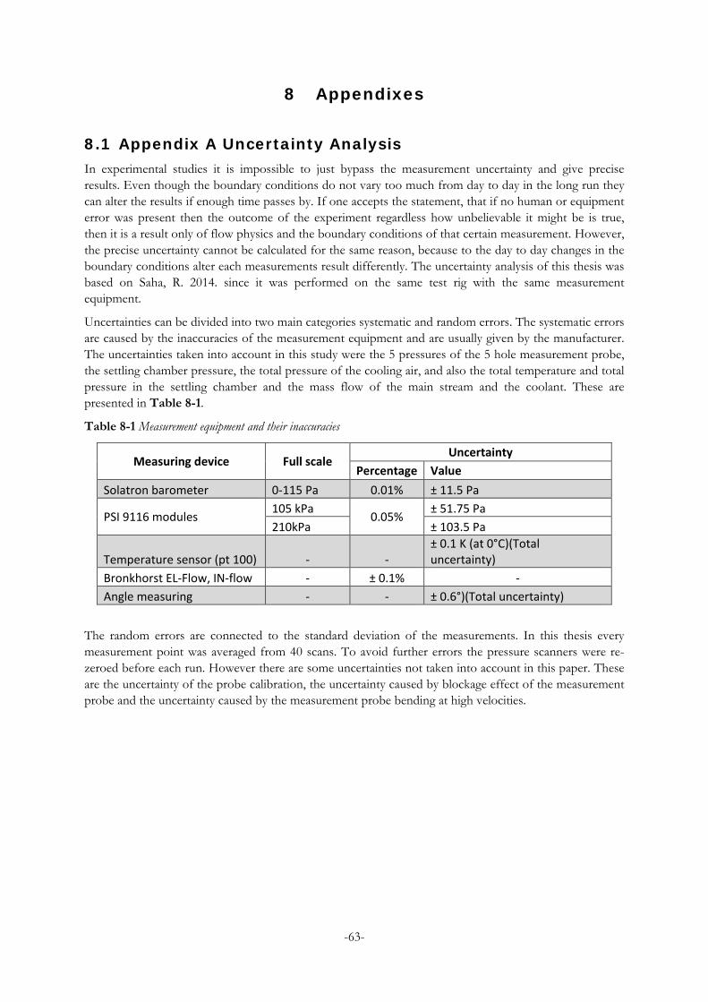
-63-

8 Appendixes

8.1 Appendix A Uncertainty Analysis In experimental studies it is impossible to just bypass the measurement uncertainty and give precise results. Even though the boundary conditions do not vary too much from day to day in the long run they can alter the results if enough time passes by. If one accepts the statement, that if no human or equipment error was present then the outcome of the experiment regardless how unbelievable it might be is true, then it is a result only of flow physics and the boundary conditions of that certain measurement. However, the precise uncertainty cannot be calculated for the same reason, because to the day to day changes in the boundary conditions alter each measurements result differently. The uncertainty analysis of this thesis was based on Saha, R. 2014. since it was performed on the same test rig with the same measurement equipment.

Uncertainties can be divided into two main categories systematic and random errors. The systematic errors are caused by the inaccuracies of the measurement equipment and are usually given by the manufacturer. The uncertainties taken into account in this study were the 5 pressures of the 5 hole measurement probe, the settling chamber pressure, the total pressure of the cooling air, and also the total temperature and total pressure in the settling chamber and the mass flow of the main stream and the coolant. These are presented in Table 8-1.

Table 8-1 Measurement equipment and their inaccuracies

Measuring device Full scale Uncertainty

Percentage Value Solatron barometer 0-115 Pa 0.01% ± 11.5 Pa

PSI 9116 modules 105 kPa

0.05% ± 51.75 Pa

210kPa ± 103.5 Pa

Temperature sensor (pt 100) - - ± 0.1 K (at 0°C)(Total uncertainty)

Bronkhorst EL-Flow, IN-flow - ± 0.1% - Angle measuring - - ± 0.6°)(Total uncertainty)

The random errors are connected to the standard deviation of the measurements. In this thesis every measurement point was averaged from 40 scans. To avoid further errors the pressure scanners were re-zeroed before each run. However there are some uncertainties not taken into account in this paper. These are the uncertainty of the probe calibration, the uncertainty caused by blockage effect of the measurement probe and the uncertainty caused by the measurement probe bending at high velocities.

-64-

8.2 Appendix B Details of Area Traverse In order to explore the detailed flow field within the scope of the present investigation, area traverse measurements were performed using pneumatic probes upstream and downstream of the NGV together with spatially fixed measuring points in the cascade flow path. For uncooled and cooled NGV loss calculations, the flow was assumed to be adiabatic and approximately the same free-stream and cooling air temperature. The various angle definitions used in the thesis are based on Figure 9-1.

Figure 9-1 Definition of pitch and yaw angle (adapted from Pütz, 2010)

A probe head coordinate system x, y, z were introduced to define the pitch angle and yaw angle. As can be seen in Figure 9-1, x is the nominal flow direction with α = 16.05°, i.e. the exit angle (sometimes also called yaw angle) the NGV designed for. z is parallel to the radius of the probe head position. The α angle is the angle between the radial projection of the local flow vector and a circumference at probe head position. The pitch angle (βacq) that is acquired from the probe pressure data and calibration curves need to be corrected due to the annular geometry of the test section and the geometry of the L-probe using simple trigonometric relations. To evaluate the data the technical computing tool Matlab® was used. For the flow vector and vorticity analysis, αref is used and it is defined as the angle between the flow and nominal direction.

In order to infer the relative strengths of vortices, it would require measurements in two closely spaced planes to obtain all three components of vortices. However, simplified expressions derive from the incompressible Helmholtz equation (Gregory-Smith et al., 1988) can be used to obtain approximate values of all three components from the data in one plane. The approach uses the measured total pressure distribution in addition to the component of the velocity. For flow vector analysis, the radial and circumferential part of the velocity vector (uz and uy) are determined by

𝐴𝑦 = 𝐴 ∗ 𝐼𝑒𝑘α𝑟𝑟𝑟

𝐴𝑧 = 𝐴 ∗ 𝐼𝑒𝑘𝑠

-65-

The axial component of the vorticity (ωx) can be calculated as:

𝜔𝑚 =𝜕𝐴𝑧𝜕𝑒

−𝜕𝐴𝑦𝜕𝜕

The front view of 5-hole probe tip and definition of the yaw and pitch planes for the calibration are depicted in Figure 9-2. The calibration of the 3-hole probe was performed in-house in a semi open calibration nozzle (Vogt and Fridh, 2005). The probe was fixed to a traverse mechanism which was instructed to provide orientation of the probe head from yaw angles ± 24 and pitch angles ± 24. For flow field measurements, the total pressure, static pressure, tangential (yaw) flow angle, radial flow angle (pitch) and Mach numbers were reconstructed at each point iteratively using an in-house designed Matlab routine (Vogt and Fridh, 2005 and Fridh, 2010).

Figure 9-2 Yaw and pitch angles defined by five-hole probe (left), front view of the 5-hole probe head

The ASC was equipped with a fully automatic traverse mechanism which is able to scan the upstream and downstream flow field. The mechanism is depicted in Figure 9-3. Two automatic traverse units were used to control radial, circumferential and yaw motions of probes. The horizontal linear traverse unit created a linear horizontal movement which was transformed to circumferential movement by a pin-connection and the rails, which guided the carts. A second traverse unit was attached to the cart in order to adjust the radial and yaw position.

-66-

Figure 9-3 Traverse system (Glodic, 2008)

A digital protractor was placed on the cart to read the angular position. The cart was equipped with an angle measuring unit and a probe tower where the probe was fastened. The angle measuring unit has an accuracy of 0.01 degrees and was used for calculating of the absolute position of the cart and the probe in already defined cylindrical coordinate systems. The probe tower allowed changing the probe position by moving it in radial direction as well as changing its yaw angle. The cart had roll-bearing wheels that rolled on the outer circumferential of the test sector. Cart rails hold the cart in the right axial position. The pneumatic probe was guided by a Teflon support sleeve, which was connected to the cart by a Teflon arc which was able to slide back and forth on the test sector.