Embed Size (px)
Citation preview
EXPERIMENTAL MEASUREMENT OF RADIATION
HEAT TRANSFER FROM COMPLEX
FENESTRATION SYSTEMS
By
BARRY ALLAN WILSON
Bachelor of Science
Oklahoma State University
Stillwater, Oklahoma
2005
Submitted to the Faculty of theGraduate College of the
Oklahoma State Universityin partial fulfillment of
the requirements forthe Degree of
MASTER OF SCIENCEMay, 2007

UMI Number: 1443031
14430312007
UMI MicroformCopyright
All rights reserved. This microform edition is protected against unauthorized copying under Title 17, United States Code.
ProQuest Information and Learning Company 300 North Zeeb Road
P.O. Box 1346 Ann Arbor, MI 48106-1346
by ProQuest Information and Learning Company.
ii
EXPERIMENTAL MEASUREMENT OF RADIATION
HEAT TRANSFER FROM COMPLEX
FENESTRATION SYSTEMS
Thesis Approved:
Dr. Dan FisherThesis Adviser
Dr. Jeffrey Spitler
Dr. Lorenzo Cremaschi
Dr. A. Gordon EmslieDean of the Graduate College
iii
ACKNOWLEDGEMENTS
First, I would like to recognize my late father Ted Wilson and late grandparents
Webster and Lois Allan, who taught me to set lofty goals and always give my best. And
although your lives were not long enough to see this day, it has been my constant drive to
make you proud that has gotten me where I am today.
I would like to give my sincere gratitude for my advisor Dr. Dan Fisher, whose overly
optimistic attitude and extreme accessibility made every problem seem surmountable.
His continuous advice and guidance was extremely helpful through this process, I only
wish I would have listened to it more often. I would also like to thank my committee
members Dr. Jeffrey Spitler and Dr. Lorenzo Cremaschi for their guidance on my work.
I would also like to thank my friends in the BACTL, Chanvit Chantrasrisalai, Chris
Carroll and Sankaranarayanan Padhmanabhan, without their continued help this thesis
truly would not have been possible. Kyong Edwards, John Gage and Jerry Dale also
provided their time and many talents through the course of this project. I would like to
recognize my colleagues in ATRC 337, ERL 110 and in my courses for providing their
advice, help and friendship.
I have always been a believer in the old proverb “We have no friends, We have no
enemies, We have only teachers.” Therefore, I would like to take this opportunity to
thank some of the great teachers in my life: Matt Youngblood, Brent Wilson, Phillip
iv
White, Colin Eddy, Bob and Kris Richey, John and Carmen Rutherford, Frank and Sheri
Capps, Penny Crofford, Sherry Bass and Carrie Witham.
I would also like to thank my entire family, who are always willing to give advice and
time whenever I am in need, and my beautiful wife Jennifer for her constant
encouragement and understanding through this process. Finally, I would like to thank the
one person I have always admired and respected the most, my mother Susan Wilson, who
through immense adversity taught me every lesson I have ever truly needed to know.
From the time I was a little kid I have hoped to one day be as intelligent and as good of a
person as you are, unfortunately I still have a long way to go.
v
TABLE OF CONTENTS
Chapter Page
Nomenclature..................................................................................................................... xiEnglish Letter Symbols.................................................................................................. xiGreek Letter Symbols .................................................................................................. xiii
1 Introduction................................................................................................................. 11.1 Background – Significance ................................................................................. 11.2 Thesis Scope ....................................................................................................... 3
2 Literature Review........................................................................................................ 52.1 LBNL (Klems) .................................................................................................... 52.2 Experiments at Queen’s & Ryerson Polytechnic Universities ........................... 7
2.2.1 Laboratory Studies ...................................................................................... 72.2.2 Calorimetric Studies.................................................................................. 11
3 Description of Experimental Facility........................................................................ 143.1 Overall Design and Capabilities ....................................................................... 143.2 Room Configuration ......................................................................................... 173.3 Heated Window Panel....................................................................................... 213.4 Heated Blinds.................................................................................................... 23
4 Calculations, Instrumentation and Experimental Uncertainty .................................. 254.1 Calculations....................................................................................................... 25
4.1.1 Heat Balance Calculations ........................................................................ 254.1.2 Convective/Radiative Split Calculations .................................................. 274.1.3 Convection Coefficient Calculations ........................................................ 284.1.4 Thermal Conductance Calculations .......................................................... 314.1.5 Calculation of Experimental Uncertainties ............................................... 31
4.2 Primary Measurements and Uncertainty........................................................... 324.2.1 Data Acquisition Unit ............................................................................... 324.2.2 Temperature Measurements...................................................................... 33
4.2.2.1 Room Surfaces.......................................................................................334.2.2.2 Window Surface ....................................................................................354.2.2.3 Window Guard Panel.............................................................................374.2.2.4 Blinds.....................................................................................................374.2.2.5 Air ..........................................................................................................384.2.2.6 Guard Space...........................................................................................39
4.2.3 Power Measurements ................................................................................ 404.2.4 Radiant Heat Flux ..................................................................................... 424.2.5 Pressure ..................................................................................................... 444.2.6 Airflow Speed ........................................................................................... 44
vi
4.3 Uncertainties in Intermediate Variables............................................................ 454.3.1 Room Airflow Rate................................................................................... 454.3.2 Heat Extraction Rate ................................................................................. 464.3.3 Radiant Heat Gains ................................................................................... 474.3.4 Total Fenestration Heat Gain .................................................................... 494.3.5 Convective Heat Gain ............................................................................... 494.3.6 Fictitious Fenestration Surface Temperature ............................................ 49
4.4 Propagation of Uncertainty Analysis to Results ............................................... 514.4.1 Radiative/Convective Split ....................................................................... 514.4.2 Convection Coefficient ............................................................................. 524.4.3 Thermal Conductance ............................................................................... 52
4.5 Validation of Experimental Facility.................................................................. 535 Experimental Procedure............................................................................................ 57
5.1 Test Procedure .................................................................................................. 575.2 Parametric Simulation Set................................................................................. 59
6 Results....................................................................................................................... 626.1 Flow Field Analysis .......................................................................................... 626.2 Heat Transfer Analysis ..................................................................................... 736.3 Assessment of the Facility and Experimental Procedure.................................. 79
7 Conclusions............................................................................................................... 827.1 Assessment of the Results................................................................................. 827.2 Future Work and Recommendations ................................................................ 83
7.2.1 Facility ...................................................................................................... 847.2.2 Instrumentation ......................................................................................... 85
References......................................................................................................................... 86Appendix A: Standard Operating Procedures................................................................... 91Appendix B: Maintenance Procedures.............................................................................. 97Appendix C: Troubleshooting......................................................................................... 103Appendix D: Facility Pictures......................................................................................... 110Appendix E: Thermocouple Calibration Summary ........................................................ 116Appendix F: DAQ Unit Channels................................................................................... 118Appendix G: Computer Control Board Channels ........................................................... 122Appendix H: HVAC System Diagrams .......................................................................... 124

vii
LIST OF TABLES
Table 2-1 Final results from Machin et al (1998) ............................................................ 10
Table 2-2 Final results from Duarte et al (2001) .............................................................. 11
Table 5-1 Parameters for the 52 experiments ................................................................... 60
Table 6-1 Radiative fractions, uncertainty and parameters for each test .......................... 75
Table E-1 Thermocouple calibration summary (Chantrasrisalai 2007b)........................ 117
Table F-1 Fluke channel configuration (Chantrasrisalai 2007b) .................................... 118
Table G-1 DAC channel diagram (Chantrasrisalai 2007b)............................................. 122
Table G-2 DAS channel layout (Chantrasrisalai 2007b) – Note the safety board channels
are in identical order as channels 51-70.......................................................................... 123
viii
LIST OF FIGURES
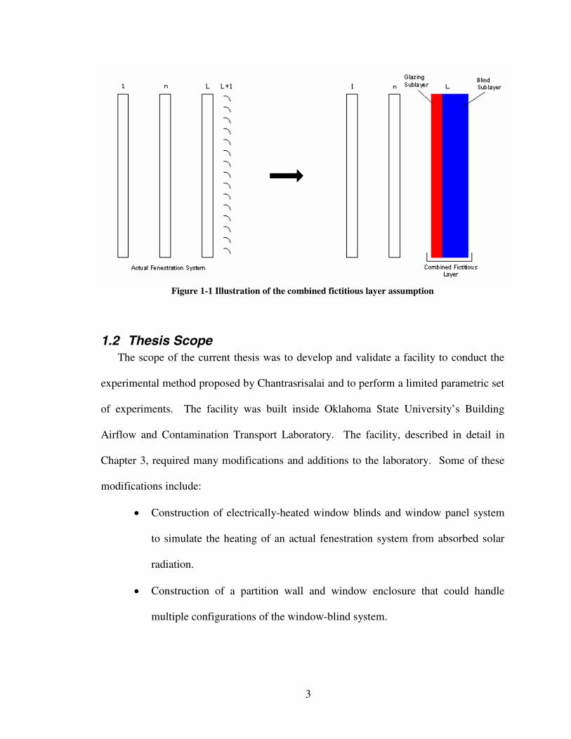
Figure 1-1 Illustration of the combined fictitious layer assumption................................... 3
Figure 2-1 Sketch of the experimental model at Queen’s University (Machin et al. 1998)8
Figure 3-1 Isometric sketch of Building Airflow and Contaminant Transport Test Rooms
(Fisher and Chantrasrisalai 2006) ..................................................................................... 15
Figure 3-2 Elevation view of the air handling system (Fisher and Chantrasrisalai 2006) 16
Figure 3-3 Layout view of the modified lower zone ........................................................ 18
Figure 3-4 Side view of the window enclosure design ..................................................... 19
Figure 3-5 Ceiling/Airflow configuration #1.................................................................... 20
Figure 3-6 Ceiling/Airflow configuration #2.................................................................... 21
Figure 3-7 Construction of heated window panel system................................................. 22
Figure 4-1 Location of thermocouples on the window panel ........................................... 36
Figure 4-2 Traversing mechanism used for net radiation and airspeed measurements .... 43
Figure 4-3 Sensitivity of the radiant gain to measurement grid density (Chantrasrisalai
2007b) ............................................................................................................................... 48
Figure 4-4 Validation of measured radiant heat gain (Chantrasrisalai 2007a) ................. 54
Figure 4-5 Validation of calculated window surface temperature (Chantrasrisalai 2007a)
........................................................................................................................................... 55
Figure 4-6 Repeatability of the radiant fraction................................................................ 56
Figure 4-7 Repeatability of the equivalent convection coefficient (based on supply air
temperature) ...................................................................................................................... 56
ix
Figure 5-1 Illustration of the three different gap-widths, from left to right 0.5 in. (12.7
mm), 1.75 in. (44.5 mm) and 3.75 in. (95.25 mm) ........................................................... 61
Figure 5-2 Illustration of the three different blind slat angles, from left to right -45°, 0º
and 45° .............................................................................................................................. 61
Figure 6-1 Airspeed [ft/min] distribution in front of and immediately above the
fenestration system for zero system airflow ..................................................................... 64
Figure 6-2 Temperature profile of fenestration system with zero system airflow............ 65
Figure 6-3 Airspeed [ft/min] distribution for 5 ACH from radial diffuser, no fenestration
power dissipation .............................................................................................................. 66
Figure 6-4 Airspeed [ft/min] distribution for 10 ACH from radial diffuser, no fenestration
power dissipation .............................................................................................................. 67
Figure 6-5 Airspeed [ft/min] distribution for 5 ACH from linear slot diffuser ................ 69
Figure 6-6 Temperature profile of fenestration system for 5 ACH from linear slot diffuser
........................................................................................................................................... 69
Figure 6-7 Airspeed [ft/min] distribution for 10 ACH from linear slot diffuser .............. 71
Figure 6-8 Temperature profile of fenestration system for 10 ACH from linear slot
diffuser .............................................................................................................................. 72
Figure 6-9 Sketch of the wall jet separation point ............................................................ 72
Figure 6-10 Effect of various parameters on radiant fraction, high power = 150W, low
power = 50W from each fenestration component............................................................. 76
Figure 6-11 Effect of component power dissipation on the radiant fraction for different
slat angles and system airflow rates.................................................................................. 76
x
Figure 6-12 Radiative fraction for various slat angles and airflow configurations with a
gap width of 0.5 in. ........................................................................................................... 78
Figure 6-13 Radiative fraction for various gap widths and airflow configurations.......... 79
Figure D-1 Tank fill/drain line filters and valves ........................................................... 110
Figure D-2 Tank side of the fill/drain line ...................................................................... 111
Figure D-3 Air filter housing before main cooling coil .................................................. 111
Figure D-4 Air filter housing on third level.................................................................... 112
Figure D-5 Variable transformer bank............................................................................ 112
Figure D-6 Cooling coil condensate drain fill pipe ........................................................ 113
Figure D-7 Safety boards ................................................................................................ 114
Figure D-8 Location of the master relay......................................................................... 114
Figure D-9 Rack mount .................................................................................................. 115
Figure H-1 System diagram for the NE fan coil unit loop (Chantrasrisalai 2007b) ....... 124
Figure H-2 System diagram for the SW fan coil unit loop (Chantrasrisalai 2007b) ...... 125
Figure H-3 System diagram for the air handler unit loop (Chantrasrisalai 2007b) ........ 126
Figure H-4 System diagram for the heat pump loops (Chantrasrisalai 2007b) .............. 127

xi
Nomenclature
English Letter Symbols
A Area
1A Plane area of the fenestration system
ACH Room air changes per hour
Lc Thermal conductance of innermost glazing layer
1+Lc Thermal conductance of the fictitious layer
pC Specific heat of air
DAQ Data acquisition unit
jbE ,Black-body emissive power of the surface j
kF −1View factor from the fictitious surface to the room surface k
convfenF ,Fraction of fenestration heat gain transferred through convection
radfenF ,Fraction of fenestration heat gain transferred through thermalradiation
kjF − View factor from surface j to surface k
FS Full-scale
fenh Fenestration convection coefficient
HVAC Heating, Ventilation and Air conditioning systemJ Radiosity
am& Mass flow rate of air
Q Room volumetric flow rate
condq& Conduction heat loss through zone surfaces
errorq& Heat balance error
totfenq ,& Power input to the fenestration system
radfenq ,& Total radiative heat transfer rate from fenestration system
plugq& Power input to the plug load
iradq ,& Net radiative heat flux at a given measurement location
spaceq& Zone heat extraction rate
wdq& Power dissipated by the heat window panel
1T Temperature of the fictitious fenestration surface temperature
raT Temperature of air at the return grill
refT Reference air temperature
xii
saT Temperature of air at the supply diffuser
insurfT ,Temperature of the inside surface
outsurfT ,Temperature of the outside (guard space side) surface
wdT Temperature of the innermost glazing layer
U Estimated overall heat transfer coefficient of surface
Au Uncertainty in flow nozzle area
cu Uncertainty in flow nozzle discharge coefficient
fu Uncertainty in differential pressure measurement
convfenFu,
Uncertainty in the convective fraction
radfenFu,
Uncertainty in the radiative fraction
mu Total uncertainty in primary measurements
imu ,Uncertainty caused by individual sources
Nu Uncertainty caused by variations in the fan speed
Qu Total uncertainty in airflow rate
inpblqu,&
Uncertainty in blind power dissipation
qu & Uncertainty in 1T due to the uncertainty in the net radiant heat gain
condqu &Uncertainty in conduction heat transfer rate
extqu &Uncertainty in heat extraction rate
convfenqu,&
Uncertainty in the convective heat gain
radfenqu,&
Uncertainty in radiant heat gain from the fenestration system
totfenqu,&
Uncertainty in total fenestration heat gain
radqu &Uncertainty in net radiant heat gain
iradqu,′′ Uncertainty in net radiant heat flux
inpwdqu,&
Uncertainty in window panel power dissipation
Tu Uncertainty in 1T due to the uncertainty in the room surfacetemperatures
1Tu Uncertainty in the fictitious fenestration surface temperature
nTTu Uncertainty of the surface temperature of the nth room surface
1εTu Uncertainty due to the propagation of the uncertainty of theemissivity of the fictitious surface
yu Uncertainty in derived variable
condTu∆ Uncertainty in the difference between inside surface temperature andguard space air temperature
extTu∆ Uncertainty in temperature difference
εu Uncertainty in 1T due to the uncertainty in the room surface
xiii
emissivities
1εu Uncertainty in the emissivity of the fictitious surface
ρu Uncertainty in air density
Greek Letter Symbols
extT∆ Difference between entering and leaving air temperatures
reffenT −∆ Difference between fictitious surface temperature and the reference
wdfenT −∆ Difference between fictitious surface temperature and the temperatureof the window panel
jε Emissivity of the inside surface j
σ Stefan-Boltzmann constant

1
1 Introduction
1.1 Background – SignificanceVenetian blinds are a very common window-shading device to provide privacy and
daylighting control; they can be found in the majority of households and many
commercial buildings. Although Venetian blinds are a very common device, their effect
on cooling and heating loads is very complicated and is not currently completely
understood. The complications come from the fact that the blinds themselves are
partially specular and partially diffuse in the visible spectrum and affect the local airflow
differently depending on the absorbed solar radiation. Furthermore, these effects can be
modified at any time by the user. Due to these complexities Venetian blinds are likely
the most common building envelope element that does not have a suitable simulation
model.
Although several simulation models have been proposed in the literature (Klems
1994a; 1994b; Klems et al. 1995b; Ye et al. 1999; Phillips et al. 2001; Naylor et al. 2002;
Naylor et al. 2006; DOE 2007), they have all been hampered by the lack of experimental
investigations into their required parameters. The experiments that have been performed
have been very complex and expensive to run resulting in little usable data. The previous
experiments were also conducted with only buoyancy driven airflows and the
experimental setup was isolated from all other airflows. Since only natural convection
was considered in previous experimental studies, it is likely that their results are
2
unrealistic due to the fact that blinds in conditioned zones are usually exposed to either
wall jets or free jets.
Due to the continued tightening of energy standards such as ASHRAE’s Standard
90.1, the desire for accurate energy simulations has increased in recent years. In order to
meet this desire, Chantrasrisalai (2007a) recently developed a new model to describe
Venetian blinds. The Chantrasrisalai model proposed that the innermost glazing surface
and the blinds be modeled as one ‘fictitious’ layer. This fictitious layer consists of two
sublayers; the back sublayer is the (real) innermost glazing while the front sublayer is
comprised of the blinds and the air gap between the two real layers as illustrated in Figure
1-1. It is further assumed that the two sublayers are in perfect thermal contact and the
layer has a thermal conductance of 1+Lc , which must be found experimentally. Utilizing
the ‘fictitious layer’ simplification, it was possible to develop a straightforward
experimental method to determine the heat transfer coefficients and radiative-convective
splits needed for radiant time series (RTS) and heat balance (HBM) load calculation
methods. The complete description, development and usage of the model can be found in
the literature (Chantrasrisalai 2007a).
3
Figure 1-1 Illustration of the combined fictitious layer assumption
1.2 Thesis ScopeThe scope of the current thesis was to develop and validate a facility to conduct the
experimental method proposed by Chantrasrisalai and to perform a limited parametric set
of experiments. The facility was built inside Oklahoma State University’s Building
Airflow and Contamination Transport Laboratory. The facility, described in detail in
Chapter 3, required many modifications and additions to the laboratory. Some of these
modifications include:
• Construction of electrically-heated window blinds and window panel system
to simulate the heating of an actual fenestration system from absorbed solar
radiation.
• Construction of a partition wall and window enclosure that could handle
multiple configurations of the window-blind system.
4
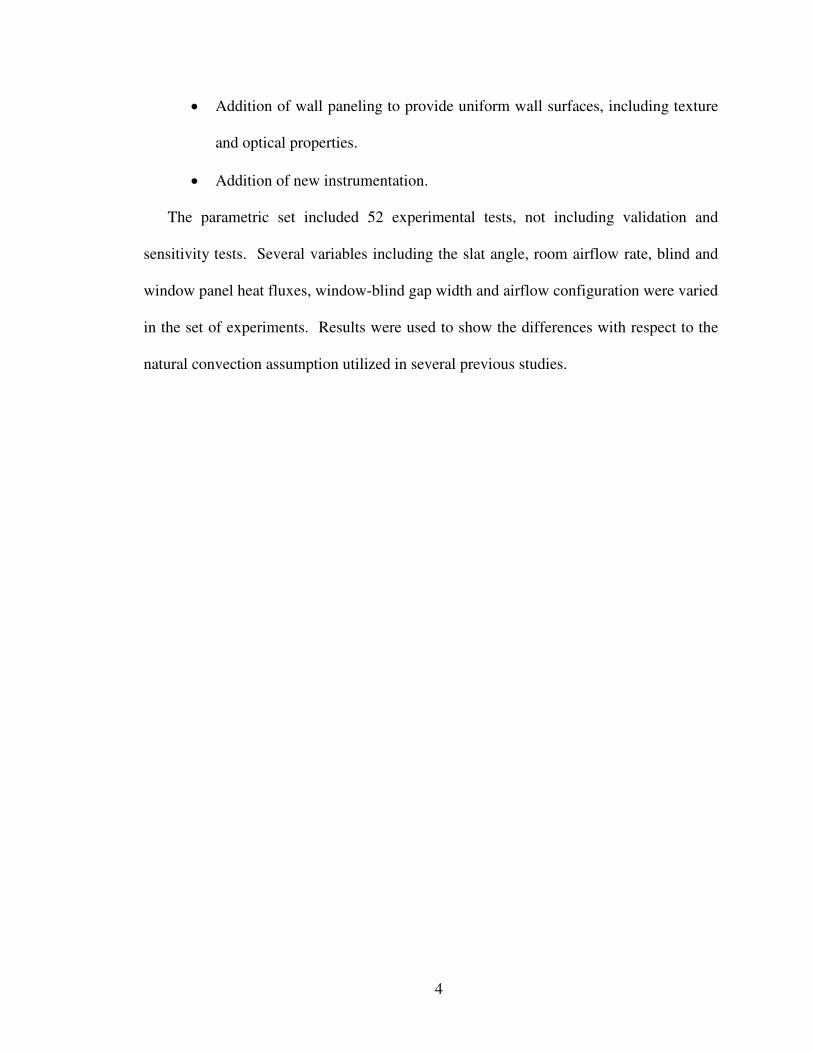
• Addition of wall paneling to provide uniform wall surfaces, including texture
and optical properties.
• Addition of new instrumentation.
The parametric set included 52 experimental tests, not including validation and
sensitivity tests. Several variables including the slat angle, room airflow rate, blind and
window panel heat fluxes, window-blind gap width and airflow configuration were varied
in the set of experiments. Results were used to show the differences with respect to the
natural convection assumption utilized in several previous studies.
5
2 Literature Review
Although there has been a great deal of theoretical and numerical research into the
effects of complex fenestration systems (Klems 1994a; 1994b; Klems et al. 1995b; Ye et
al. 1999; Oh et al. 2001; Phillips et al. 2001; Naylor et al. 2002; 2006), there has been
very little recent experimental work on the subject. All of the recent experimental
research was conducted at Lawrence Berkeley Nation Laboratory (LBNL) and a group of
Canadian universities including Queen’s, Ryerson Polytechnic and Waterloo. Although
the researchers produced reasonable and consistent results, they all made a major
assumption – that convection was driven by buoyancy effects only. This assumption is
likely to be unrealistic considering that a shading layer in an actual building will be
exposed to air currents and many are adjacent to slot diffusers. The experimental work of
these two groups will be analyzed in detail in the following sections.
2.1 LBNL (Klems)In the mid-1990s, Klems et al. developed a model to predict the effects of shading on
solar heat gains. The model was based on two concepts: First, the optical properties of
the system were considered a function of the optical properties of each glazing or shading
layer. Second, the inward flowing fraction was considered solely a thermal property of
each layer independently of the layer’s optical properties (Klems 1994a; 1994b; Klems et
al. 1995b).
6
Experimental research at LBNL supported their model and provided reference data
suitable for a handbook. In 1995, Klems and Warner published a paper detailing a
method to determine the bidirectional optical properties of shading devices utilizing a
scanning radiometer. They validated their method by determining the optical properties
of a Venetian blind, one of the most optically complex shading devices available, and
showed their method was significantly quicker than calorimetric measurements (Klems
and Warner 1995a).
In 1996, Klems and Kelley produced a method for determining the inward-flowing
fraction through calorimetric studies. By utilizing a dual chamber calorimeter where both
chambers had an identical setup, they were able to determine the shading layer’s specific
inward-flowing fraction by slightly heating the shading device in one chamber. Using
this method they found the inward flowing fraction for a limited set of configurations
(Klems and Kelley 1996). A correlation for the inward-flowing fraction was later
developed for Venetian blinds (Collins and Harrison 1999).
The results of the previous two papers were brought together in 1997 to show the
utility of the model the researchers had developed. They determined that the model, with
the experimental results, provided a reasonable picture of the performance of a complex
fenestration system (Klems and Warner 1997). However, this model has not been widely
used because of the lack of a database containing the optical and thermal properties of
various shading layers.
7
2.2 Experiments at Queen’s & Ryerson Polytechnic Universities
2.2.1 Laboratory StudiesAt Queen’s and Ryerson Polytechnic Universities in Ontario, Canada, work has
centered on modeling heat transfer from the blinds using finite element methods. Both
research groups experimentally validated their models.
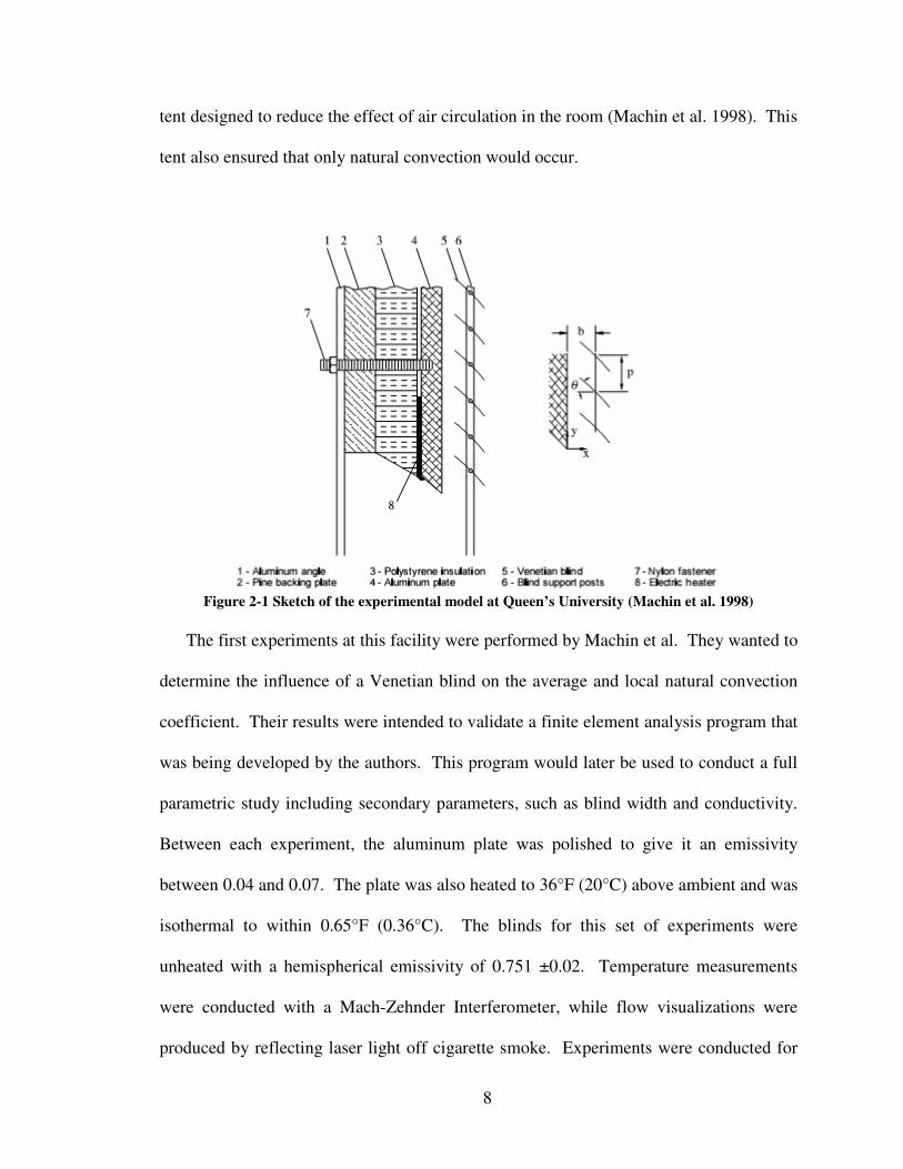
The facility at Queen’s consisted of a Venetian blind placed in front of a vertical plate
that represented the inner pane of a fenestration system. A sketch of the facility is shown
in Figure 2-1. In earlier studies the vertical panel was heated with electrical strip heaters,
while later studies heated and cooled the panel utilizing hydraulic flow channels (Machin
et al. 1998; Collins et al. 2001). The plate was precision ground and had a beveled
bottom edge to promote ideal boundary layer formation (Machin et al. 1998).
Temperature within the plate was measured with ten 24-gauge copper-constantan
thermocouples, and one platinum RTD sensor that were placed in holes drilled on the
backside of the plate to within .08in (2mm) of the surface. The leading edge temperature
was measured with one 40-gauge thermocouple placed 0.20in (5mm) from the tip
(Machin et al. 1998).
The Venetian blinds also matured in later studies, the original setup utilized
unheated blind slats while later studies heated the slats with two foil heating strips
bonded to the concave surface of the slats (Machin et al. 1998; Collins et al. 2001). In all
experiments the slats were taken from a commercially available aluminum Venetian blind
set. The emissivity of the slats and vertical plate were modified for the given
experiments.
To allow for interferometer measurements an optical window constructed from
plexiglass was placed on either side of the setup. The setup was also covered in a large
8
tent designed to reduce the effect of air circulation in the room (Machin et al. 1998). This
tent also ensured that only natural convection would occur.
Figure 2-1 Sketch of the experimental model at Queen’s University (Machin et al. 1998)
The first experiments at this facility were performed by Machin et al. They wanted to
determine the influence of a Venetian blind on the average and local natural convection
coefficient. Their results were intended to validate a finite element analysis program that
was being developed by the authors. This program would later be used to conduct a full
parametric study including secondary parameters, such as blind width and conductivity.
Between each experiment, the aluminum plate was polished to give it an emissivity
between 0.04 and 0.07. The plate was also heated to 36°F (20°C) above ambient and was
isothermal to within 0.65°F (0.36°C). The blinds for this set of experiments were
unheated with a hemispherical emissivity of 0.751 ±0.02. Temperature measurements
were conducted with a Mach-Zehnder Interferometer, while flow visualizations were
produced by reflecting laser light off cigarette smoke. Experiments were conducted for
9
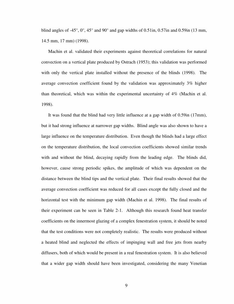
blind angles of -45°, 0°, 45° and 90° and gap widths of 0.51in, 0.57in and 0.59in (13 mm,
14.5 mm, 17 mm) (1998).
Machin et al. validated their experiments against theoretical correlations for natural
convection on a vertical plate produced by Ostrach (1953); this validation was performed
with only the vertical plate installed without the presence of the blinds (1998). The
average convection coefficient found by the validation was approximately 3% higher
than theoretical, which was within the experimental uncertainty of 4% (Machin et al.
1998).
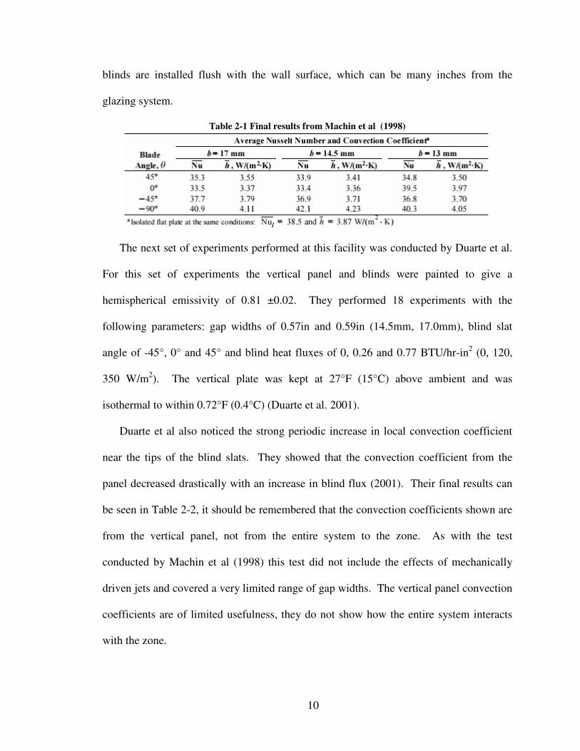
It was found that the blind had very little influence at a gap width of 0.59in (17mm),
but it had strong influence at narrower gap widths. Blind angle was also shown to have a
large influence on the temperature distribution. Even though the blinds had a large effect
on the temperature distribution, the local convection coefficients showed similar trends
with and without the blind, decaying rapidly from the leading edge. The blinds did,
however, cause strong periodic spikes, the amplitude of which was dependent on the
distance between the blind tips and the vertical plate. Their final results showed that the
average convection coefficient was reduced for all cases except the fully closed and the
horizontal test with the minimum gap width (Machin et al. 1998). The final results of
their experiment can be seen in Table 2-1. Although this research found heat transfer
coefficients on the innermost glazing of a complex fenestration system, it should be noted
that the test conditions were not completely realistic. The results were produced without
a heated blind and neglected the effects of impinging wall and free jets from nearby
diffusers, both of which would be present in a real fenestration system. It is also believed
that a wider gap width should have been investigated, considering the many Venetian
10
blinds are installed flush with the wall surface, which can be many inches from the
glazing system.
Table 2-1 Final results from Machin et al (1998)
The next set of experiments performed at this facility was conducted by Duarte et al.
For this set of experiments the vertical panel and blinds were painted to give a
hemispherical emissivity of 0.81 ±0.02. They performed 18 experiments with the
following parameters: gap widths of 0.57in and 0.59in (14.5mm, 17.0mm), blind slat
angle of -45°, 0° and 45° and blind heat fluxes of 0, 0.26 and 0.77 BTU/hr-in2 (0, 120,
350 W/m2). The vertical plate was kept at 27°F (15°C) above ambient and was
isothermal to within 0.72°F (0.4°C) (Duarte et al. 2001).
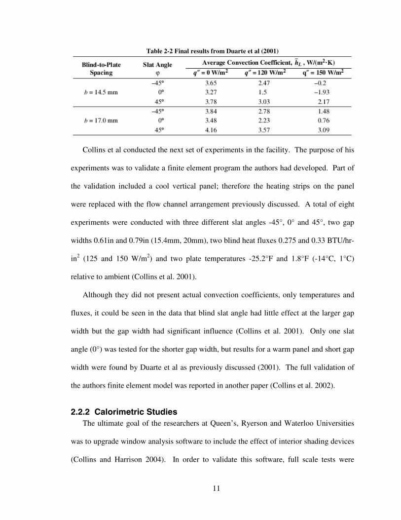
Duarte et al also noticed the strong periodic increase in local convection coefficient
near the tips of the blind slats. They showed that the convection coefficient from the
panel decreased drastically with an increase in blind flux (2001). Their final results can
be seen in Table 2-2, it should be remembered that the convection coefficients shown are
from the vertical panel, not from the entire system to the zone. As with the test
conducted by Machin et al (1998) this test did not include the effects of mechanically
driven jets and covered a very limited range of gap widths. The vertical panel convection
coefficients are of limited usefulness, they do not show how the entire system interacts
with the zone.
11
Table 2-2 Final results from Duarte et al (2001)
Collins et al conducted the next set of experiments in the facility. The purpose of his
experiments was to validate a finite element program the authors had developed. Part of
the validation included a cool vertical panel; therefore the heating strips on the panel
were replaced with the flow channel arrangement previously discussed. A total of eight
experiments were conducted with three different slat angles -45°, 0° and 45°, two gap
widths 0.61in and 0.79in (15.4mm, 20mm), two blind heat fluxes 0.275 and 0.33 BTU/hr-
in2 (125 and 150 W/m2) and two plate temperatures -25.2°F and 1.8°F (-14°C, 1°C)
relative to ambient (Collins et al. 2001).
Although they did not present actual convection coefficients, only temperatures and
fluxes, it could be seen in the data that blind slat angle had little effect at the larger gap
width but the gap width had significant influence (Collins et al. 2001). Only one slat
angle (0°) was tested for the shorter gap width, but results for a warm panel and short gap
width were found by Duarte et al as previously discussed (2001). The full validation of
the authors finite element model was reported in another paper (Collins et al. 2002).
2.2.2 Calorimetric StudiesThe ultimate goal of the researchers at Queen’s, Ryerson and Waterloo Universities
was to upgrade window analysis software to include the effect of interior shading devices
(Collins and Harrison 2004). In order to validate this software, full scale tests were
12
performed utilizing a solar calorimeter located at Queen’s University. Twelve tests were
performed with one glazing system, two sets of blinds, three blind angles -45°, 0° and 45°
and two solar profile angles of 30° and 45°. The two sets of blinds were identical except
for their color; one was painted with white enamel while the other was painted flat black.
The white and black blinds had solar absorptances of 0.32 and 0.90 and hemispherical
emissivities of 0.75 and 0.89, respectively (Collins and Harrison 2004).
Due to weather conditions and the relatively short period of the year appropriate for
solar calorimetric studies, two test configurations were not tested by Collins and
Harrison. It should be noted that multiple test runs were conducted and averaged to
produce the final results. They determined that the presence of the Venetian blinds did
not significantly affect the thermal transmission (U-factor) of the glazing systems. It did,
however, have a large impact on the solar heat gain. The black blind reduced the solar
heat gain by 5% to 10%, with the largest occurring when the blind intercepted the
majority of the solar radiation. The more reflective white blind reduced the solar heat
gain by 9% to 37%. When the blinds were set to reflect the majority of the solar
radiation there was a 37% reduction in the heat gain, the blinds at 0° achieved a 19%
reduction, even when the blinds were turned to allow in as much solar radiation as
possible they still provided a reduction of 9% (Collins and Harrison 2004).
Although the researcher produced impressive results, their experimental method still
has some flaws. First, a calorimeter has no mechanically driven airflows, thus only
natural convection occurred. Real conditions usually expose complex fenestration
systems to air currents, which could drastically increase the convection rates. Second, the
13
experimental method would be very expensive and time consuming to implement on the
scale required to produce empirical heat transfer correlations.

14
3 Description of Experimental Facility
The experimental studies for the current thesis were performed in the Building
Airflow and Contaminant Transport Laboratory at Oklahoma State University. The
experimental facility configuration and equipment are described in the following
sections.
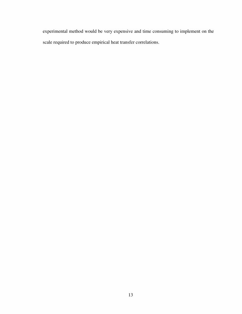
3.1 Overall Design and CapabilitiesThe experimental facility consisted of two large office sized rooms with a connecting
stairwell as shown in Figure 3-1. The test rooms were located inside a large three-story
laboratory. Although upper and lower zones are identical in size and construction, except
the upper zone only has one entry door, only the lower zone was utilized for the current
research project. Each zone had a commercially available raised flooring system as well
as a standard suspended ceiling. During tests the space surrounding the lower zone as
well as the upper and lower floor plenums were used as temperature controlled guard
spaces. These guard spaces are controlled to match the temperature within the lower
zone to prevent conduction heat transfer through the zone walls. To prevent air leakage
during experiments the lower zone was completely sealed using DOW’s ‘Seal ‘n Peel’
caulk.
The upper and lower zones were separated by 22-gauge roof decking and 3/4in
(19mm) of spray foam. The R-value for the floor construction was estimated to be 5.0°F-
ft²-hr/Btu (0.9m²-K/W) (ASHRAE 2005). The zone walls were constructed out of 2.69in
15
(68.3mm) extruded polystyrene sandwiched between two sheets of hard wall panel. The
wall construction had an approximate R-Value of 11.3°F-ft²-hr/Btu (2.0m²-K/W)
(ASHRAE 2005). The raised floor tiles were constructed out of steel clad, 1in (25.4mm)
thick OSB board. The floors were covered with linoleum tile and 1/8in (3.2mm) thick
wall board. The final construction had an approximate R-value of 2.4°F-ft²-hr/Btu
(0.4m²-K/W) (ASHRAE 2005). For the current research the standard acoustic ceiling
tiles were replaced with 1/8in (3.2mm) thick wall boards with an approximate R-value of
0.18°F-ft²-hr/Btu (0.03m²-K/W) (ASHRAE 2005).
Figure 3-1 Isometric sketch of Building Airflow and Contaminant Transport Test Rooms (Fisher and
Chantrasrisalai 2006)
16
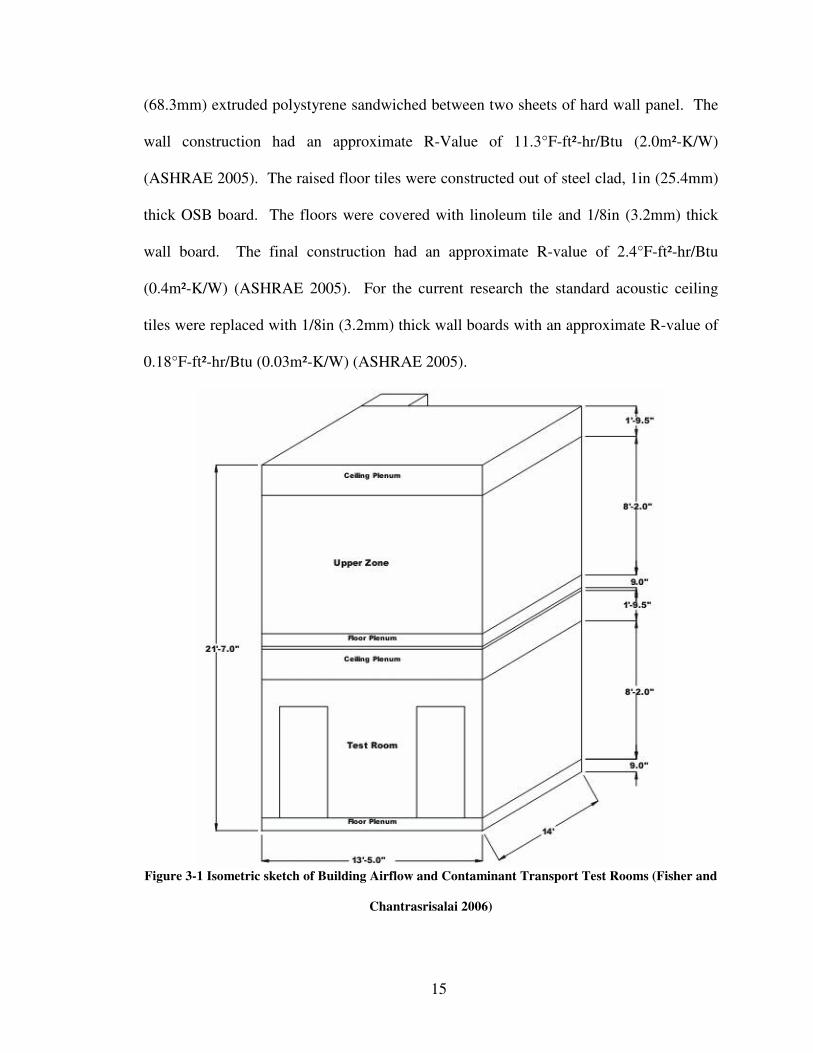
The test room was conditioned by a system that contained variable speed supply and
return fans, a mixing box, heating and cooling coils and three ASHRAE Standard flow
measurement boxes. An elevation view of the air handling system is shown in Figure
3-2. Although the current project utilized zero outside air, the system was capable of
running up to 100% outside air. To allow for parametric studies the system was designed
for quick configuration of supply and return ducts/plenums. The facility could run either
ducted or plenum supplies and returns. Detailed system schematics are presented in
Appendix H.
Figure 3-2 Elevation view of the air handling system (Fisher and Chantrasrisalai 2006)
17
The guard space was conditioned with two fan-coil units. The fan-coil units were
located in the North East corner and the South West corner of the guard space and blew
along the North and South walls, respectively. A fan was placed in each of the two
remaining corners in order to ensure a uniform temperature in the guard space. The
upper and lower floor plenums were supplied conditioned air from the main guard space.
The floor plenum supply fans also had an electric reheat coil to help maintain a proper
guard temperature.
3.2 Room ConfigurationAs previously mentioned the current project was conducted solely in the lower zone,
which was specifically configured for the project as shown in Figure 3-3. The largest
modification to the lower zone was the addition of a partition wall. This wall separated
the zone into two spaces, the larger of which became the test zone while the smaller
became a guard space. A window enclosure was framed into the center of the partition
wall; it was designed so that the gap between the heated panel, which simulated the
window glazing, and the blinds could range between 0 and 5in (130mm). A side view of
the window enclosure design is shown in Figure 3-4. The south entrance door was also
removed to allow the inner guard space to mix with the outer guard space.
The partition wall and access door were sheathed with 1/8in (3.2mm) wall board
painted with Sherwin Williams Eggshell interior latex with a known emissivity of 0.9
±0.05. The sheathing was backed with 1in (25.4mm) thick DOW blueboard insulation
for an approximate R-value of 5.2°F-ft²-hr/Btu (0.92m²-K/W) (ASHRAE 2005). The
sides and top of the window enclosure were framed out of 1/2in (12.7mm) thick
plexiglass backed with 1in (25.4mm) thick blueboard insulation resulting in an estimated
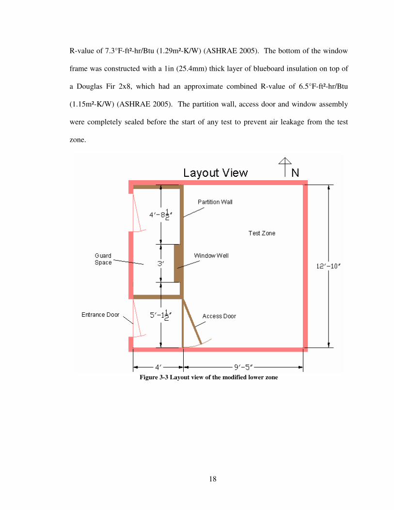
18
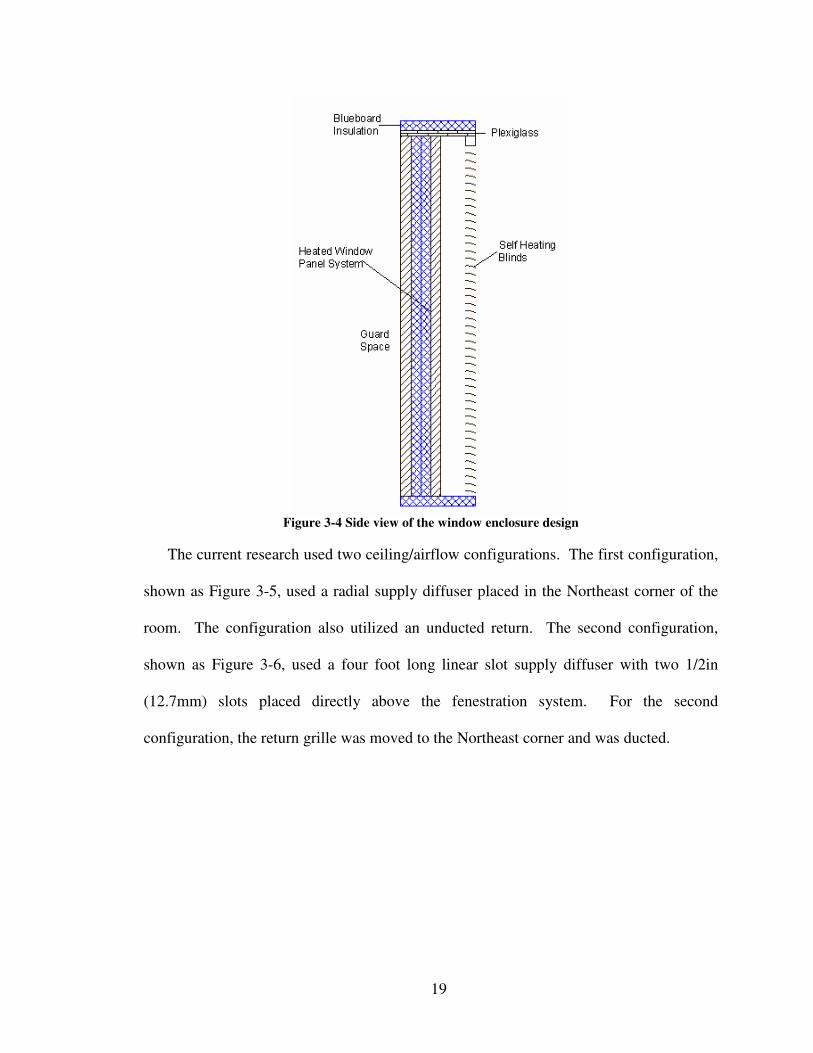
R-value of 7.3°F-ft²-hr/Btu (1.29m²-K/W) (ASHRAE 2005). The bottom of the window
frame was constructed with a 1in (25.4mm) thick layer of blueboard insulation on top of
a Douglas Fir 2x8, which had an approximate combined R-value of 6.5°F-ft²-hr/Btu
(1.15m²-K/W) (ASHRAE 2005). The partition wall, access door and window assembly
were completely sealed before the start of any test to prevent air leakage from the test
zone.
Figure 3-3 Layout view of the modified lower zone
19
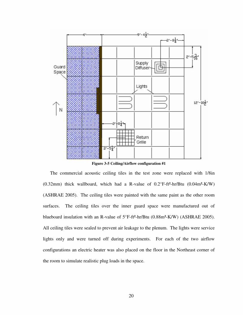
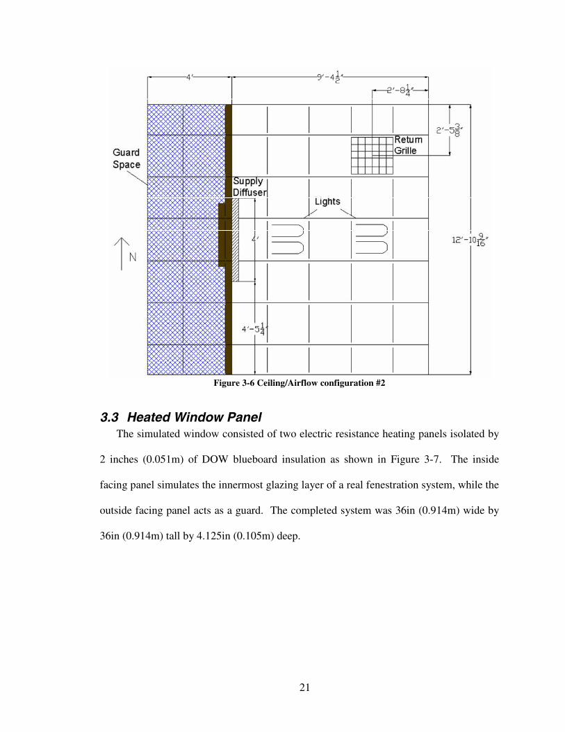
Figure 3-4 Side view of the window enclosure design
The current research used two ceiling/airflow configurations. The first configuration,
shown as Figure 3-5, used a radial supply diffuser placed in the Northeast corner of the
room. The configuration also utilized an unducted return. The second configuration,
shown as Figure 3-6, used a four foot long linear slot supply diffuser with two 1/2in
(12.7mm) slots placed directly above the fenestration system. For the second
configuration, the return grille was moved to the Northeast corner and was ducted.
20
Figure 3-5 Ceiling/Airflow configuration #1
The commercial acoustic ceiling tiles in the test zone were replaced with 1/8in
(0.32mm) thick wallboard, which had a R-value of 0.2°F-ft²-hr/Btu (0.04m²-K/W)
(ASHRAE 2005). The ceiling tiles were painted with the same paint as the other room
surfaces. The ceiling tiles over the inner guard space were manufactured out of
blueboard insulation with an R-value of 5°F-ft²-hr/Btu (0.88m²-K/W) (ASHRAE 2005).
All ceiling tiles were sealed to prevent air leakage to the plenum. The lights were service
lights only and were turned off during experiments. For each of the two airflow
configurations an electric heater was also placed on the floor in the Northeast corner of
the room to simulate realistic plug loads in the space.
21
Figure 3-6 Ceiling/Airflow configuration #2
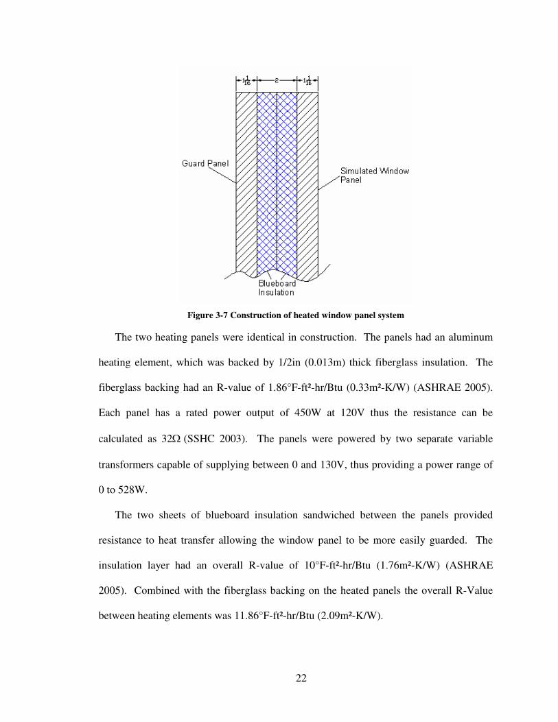
3.3 Heated Window PanelThe simulated window consisted of two electric resistance heating panels isolated by
2 inches (0.051m) of DOW blueboard insulation as shown in Figure 3-7. The inside
facing panel simulates the innermost glazing layer of a real fenestration system, while the
outside facing panel acts as a guard. The completed system was 36in (0.914m) wide by
36in (0.914m) tall by 4.125in (0.105m) deep.
22
Figure 3-7 Construction of heated window panel system
The two heating panels were identical in construction. The panels had an aluminum
heating element, which was backed by 1/2in (0.013m) thick fiberglass insulation. The
fiberglass backing had an R-value of 1.86°F-ft²-hr/Btu (0.33m²-K/W) (ASHRAE 2005).
Each panel has a rated power output of 450W at 120V thus the resistance can be
calculated as 32Ω (SSHC 2003). The panels were powered by two separate variable
transformers capable of supplying between 0 and 130V, thus providing a power range of
0 to 528W.
The two sheets of blueboard insulation sandwiched between the panels provided
resistance to heat transfer allowing the window panel to be more easily guarded. The
insulation layer had an overall R-value of 10°F-ft²-hr/Btu (1.76m²-K/W) (ASHRAE
2005). Combined with the fiberglass backing on the heated panels the overall R-Value
between heating elements was 11.86°F-ft²-hr/Btu (2.09m²-K/W).

23
To ensure that all the heat dissipated through the window panel entered the room, the
temperature gradient across the insulation layer was controlled to zero. Nine
thermocouples were placed between each panel and the connecting blueboard sheet to
facilitate the control of the temperature gradient. The temperatures were balanced by
setting the window panel to the appropriate power output and then adjusting the guard
panel power until a temperature balance was achieved.
3.4 Heated BlindsIn order to simulate blinds heated by solar radiation a set of heated window blinds
was constructed. Each slat of the blind assembly was heated by passing an electrical
current through the slat. The electrical resistance of the slat resulted in Joule heating. To
ensure realism the blinds were manufactured by modifying a commercially available set
of Venetian blinds purchased at a local hardware store. For this experiment, the overall
dimensions of the blinds were 36in (0.914m) wide by 36in (0.914m) tall by 1in (.0254m)
deep; the height included the frame of the blinds.
The stock aluminum slats from the commercial set of blinds were removed and
replaced with slats manufactured out of 26 gauge (0.4547mm) AISI Type 304 Stainless
Steel (Wilson et al. 2004). Each slat was cut to exactly 36in (0.914m) long by 1in
(.0254m) wide. To simulate the curvature of the original slats, the new slats were curved
around a die with a radius of curvature of 1.5in (0.0381m), slightly larger than original
aluminum slats but still smaller than many commercial blinds. Finally, a 1/8in
(3.175mm) hole was drilled to allow a retaining cord to be run through each slat to
prevent side-to-side movement; this hole was located at the length-wise midpoint and a
1/8in (3.175mm) from the edge. The hole’s location and size identically matched the

24
placement on the commercial blinds. In order to achieve the required height of the blind
set, 43 slats were used.
The stainless steel used to manufacture the slats had an electrical resistivity of
2.83x10⁻⁵Ohm-in (7.20x10⁻⁵Ohm-cm) (MatWeb 2006b). The electrical resistance of each
slat was found to be 63.4 mΩ. To reduce amperage requirements the 43 slats were
connected in a series circuit to provide a total slat resistance of 2.73Ω. The slats were
connected to each other with 12in (0.305m) of 14AWG high quality, car stereo, copper
wire, chosen for its low resistance and extreme flexibility. The connecting wires had a
measured resistance of roughly 0.234 mΩ/in (9.2 mΩ/m) for a total resistance of 0.125Ω.
The wire was connected to the slats utilizing a 95% Tin and 5% Silver solder which has
electrical resistivity of 4.09x10⁻⁶Ohm-in (1.04x10⁻⁵Ohm-cm) (MatWeb 2006a). Together
the system had a total resistance of 2.85Ω.
The blinds were powered utilizing an AEEC-110VAC variable transformer. The
power supply receives its power from a standard 120V wall socket and has a fused input
amperage of 15A. It can provide an output voltage between 0 and 130V and has a fused
amperage output of 20A. Utilizing this power supply the blinds can dissipate 1140W of
energy – much more than required for this experiment.
In order to decrease the uncertainty of the radiation measurements the blinds were
painted with Sherwin-Williams Eggshell interior latex with a known emissivity of 0.9
±0.05. Uncertainty calculations will be discussed in Chapter 4.

25
4 Calculations, Instrumentation and ExperimentalUncertainty
4.1 CalculationsThe calculations required to determine the primary parameters for the Chantrasrisalai
model are given in the following sections. The development of these calculations can be
found in the literature (Chantrasrisalai 2007a).
4.1.1 Heat Balance CalculationsThe experimental method proposed by Chantrasrisalai requires that all experimental
tests be conducted at steady state. A heat balance error calculation was utilized to
determine whether the experimental facility had reached steady state; surface and air
temperatures were also monitored to ensure that steady state had been obtained. The
room heat balance error was calculated utilizing equation 4-1 or as a percentage with
equation 4-2. It should be noted here that a heat balance was not required for the current
study and was only used to predict steady state conditions.
spacecondtotfenplugerror qqqqq &&&&& −−+= ∑,4-1
∑−+=
condtotfenplug
errorpcterror qqq
&&&
&&
,,
4-2
Where:
errorq& = heat balance error, in [BTU/hr] or [W]
pcterrorq ,& = heat balance error presented as a percentage [%]
plugq& = power input to the plug load, in [BTU/hr] or [W]
26
totfenq ,& = power input to the fenestration system, in [BTU/hr] or [W]
spaceq& = zone heat extraction rate, in [BTU/hr] or [W]
condq& = conduction heat loss through zone surfaces, in [BTU/hr] or [W]
The power input into the plug load, blinds and window panel were measured directly
utilizing precision watt transducers. The fenestration power was simply the sum of the
power input to the blinds and window panel.
Assuming no air infiltration into the zone, the zone heat extraction rate can be
calculated with equation 4-3.
( )saraPaspace TTCmq −⋅⋅= && 4-3
Where:
am& = mass flow rate of air, in [slug/hr] or [kg/s]
pC = specific heat of air, in [BTU/slug-°F] or [J/kg-°C]
saT = temperature of air at the supply diffuser, in [°F] or [°C]
raT = temperature of air at the return grill, in [°F] or [°C]
The heat loss from conduction through the zone surfaces was estimated with equation
4-4. The conduction through each surface was estimated independently and then
summed. The overall heat transfer coefficient included the outside air film coefficient
but not an inside air film coefficient and was estimated with literature data (ASHRAE
2005). The inside air film coefficient was not needed because inside surface
temperatures were measured.
( )outsurfinsurfcond TTAUq ,, −⋅⋅=& 4-4
Where:
27
U = estimated overall heat transfer coefficient of surface, in [BTU/ft2-°F]
or [W/m2-K]
A = surface area, in [ft2] or [m2]
insurfT ,= temperature of the inside surface, in [°F] or [°C]
outsurfT ,= film air temperature of the outside (guard space side) surface, in [°F]
or [°C]
4.1.2 Convective/Radiative Split CalculationsThe convective-radiative split is an important parameter for the radiant time series
thermal model proposed by Chantrasrisalai. As discussed in Chapter 3, electrical current
was applied to the window panel and blinds to simulate the heat gain from solar radiation
and conduction. Once the test room had reached steady state conditions, a scanning net
radiometer, discussed in section 4.2.4, measured the net radiation flux between the
fenestration system and the room surfaces. The total fenestration radiative flux was
calculated with equation 4-5.
∑=
⋅′′=n
iiiradradfen Aqq
1,,&
4-5
Where:
radfenq ,& = total radiative heat transfer rate from fenestration system, in [BTU/hr]
or [W]
iradq ,& = net radiative heat flux at a given measurement location, in [BTU/hr]
or [W]
iA = area of each measurement location, in [ft2] or [m2]
n = number of measurement locations
28
Once the net radiation transfer was determined, the convective/radiative split could be
found with equation 4-6 and 4-7. It should be noted that the calculation assumes that all
power dissipated by the fenestration system was transferred to the test room through
radiation or convection.
totfen
radfenradfen q
qF
,
,, &
&=
4-6
radfenconvfen FF ,, 1−= 4-7
Where:
radfenF ,= fraction of fenestration heat gain transferred through thermal
radiation
convfenF ,= fraction of fenestration heat gain transferred through convection
4.1.3 Convection Coefficient CalculationsThe model proposed by Chantrasrisalai combines the innermost glazing and Venetian
blind layers into a single ‘fictitious’ layer. Therefore, in order to calculate the equivalent
convection coefficient the fictitious surface temperature (FST) of this layer must be
calculated. The FST was estimated utilizing the standard net-radiation method (Incropera
and Dewitt 2002a) along with the measured net radiation and the test room surface
temperatures. The surface temperatures of the fenestration system were not required for
these calculations but they were monitored.
The basic net radiation equation for the fictitious surface is given by equation 4-8,
where the net radiation is known (measured) and surface 1 is the fictitious surface.
∑=
− ⋅−=n
kkk
radfen JFJA
q
111
1
,& 4-8
29
Where:
J = Radiosity, in [BTU/ft2] or [W/m2]
kF −1= view factor from the fictitious surface to the room surface k
1A = plane area of the fenestration system, in [ft2] or [m2]
n = number of room surfaces locations
The basic net radiation equation for the room surface j is given as equation 4-9, where
the surface temperature is known.
( ) ∑=
− ⋅−=−−
n
kkkjjjjb
j
j JFJJE1
,1 εε 4-9
Where:
jε = emissivity of the inside surface j
kjF − = view factor from surface j to surface k
jbE ,= black-body emissive power of the surface j, in [BTU/ft2] or [W/m2]
The black-body emissive power of each surface was calculated utilizing the Stefan-
Boltzmann law with the measured surface temperatures. The view factors between the
room surfaces were calculated utilizing equations for parallel and perpendicular planes.
Data supplied from the paint manufacturer was used to determine the emissivity of the
room surfaces.
Equations 4-8 and 4-9 can be written and solved in matrix form resulting in equation
4-10. The detailed solution to this matrix can be found in the literature (Chantrasrisalai
2007a).
30
4 11
,
1
11
11
+⋅
−⋅= J
A
qT radfen&
εε
σ
4-10
Where:
σ = Stefan-Boltzmann constant, 1.887x10⁻⁷ BTU-R4/hr-ft2 or 5.67x10⁻⁷
W-K4/m2
1T = fictitious fenestration surface temperature, in [°F] or [°C]
Once the fictitious surface temperature has been calculated, Newton’s law of cooling
can be utilized to determine the equivalent convection coefficient of the fictitious surface
as shown in equation 4-11.
( )ref
convfenfen TTA
qh
−⋅=
11
,& 4-11
Where:
fenh = equivalent fenestration convection coefficient, in [BTU/ft2-°F] or
[W/m2-K]
refT = reference air temperature, in [°F] or [°C]
The spatially averaged room air temperature is typically used as the reference
temperature for simulation models. However, some of the literature suggests that the
supply air temperature might be a more suitable reference temperature for convection
correlations (Fisher and Pedersen 1997). The experimental facility included both a
supply air duct, return air duct and room air thermocouples to accommodate correlations
based on different reference temperatures.
31
4.1.4 Thermal Conductance CalculationsAs previously discussed, the Chantrasrisalai model combines the innermost glazing
layer and the blinds into a single ‘fictitious’ layer. This fictitious layer is modeled as two
homogeneous layers having perfect thermal contact. The back layer represents the
glazing surface while the front layer consists of the blinds and the air separating the two
real layers. Since the model combines the innermost glazing layer and the blinds into a
single fictitious surface, it assumes that all heat transfer from the innermost glazing layer,
including convection and radiation, is conducted through the fictitious layer to the
surface. The thermal conductance of the back (glazing) layer ( Lc ) can be found in the
literature, but the conductance of the front (fictitious) layer ( 1+Lc ) must be found
experimentally. Equation 4-12 is used to determine the conductance of the front layer.
The detailed conduction modeling for this parameter can be found in the literature
(Chantrasrisalai 2007a).
( )111 TTA
qc
wd
wdL −⋅
=+
& 4-12
Where:
wdq& = power dissipated by the heat window panel, in [BTU/hr] or [W]
wdT = temperature of the innermost glazing layer, in [°F] or [°C]
4.1.5 Calculation of Experimental UncertaintiesThe accuracy of the experimental results was determined through an uncertainty
analysis based on the method presented by Kline and McClintock (1953). Uncertainty of
primary measurements is estimated as the root of the summed square error of each source
of uncertainty, as shown in equation 4-13.
32
2,
22,
21, immmm uuuu +⋅⋅⋅++= 4-13
Where:
mu = total uncertainty in the primary measurement
imu ,= uncertainty caused by individual sources
Uncertainties in the primary measurements are propagated to intermediate variables,
whose uncertainty is propagated to the final results. The current research uses the
method presented by Beckwith et al. (1993), as presented in equation 4-14, to
approximate the uncertainty in derived variables.
22
22
2
11
∂∂
+⋅⋅⋅+
∂∂
+
∂∂
= nn
y ux
yu
x
yu
x
yu
4-14
Where:
iu = uncertainty in the primary measurement (or intermediate variable) ix
yu = uncertainty in derived variable
4.2 Primary Measurements and Uncertainty
4.2.1 Data Acquisition UnitTwo Fluke 2628A data acquisition (DAQ) units with precision analog modules are
used to collect all experimental data. All channels, except the net radiometer, are
scanned once every 10 seconds and their readings are sent to the control computer. The
control program then calculates the heat balance, controls the HVAC system and shows
average temperature information. The data from every channel is written into a log file,
while the calculated values are written to a separate summary file. A sub-program is used
to perform the radiation measurements and move the traversing mechanism. The

33
radiation results are written to their own summary file for post-processing. The specific
DAQ units’ channel layouts can be found in Appendix F.
4.2.2 Temperature Measurements
4.2.2.1 Room SurfacesThe room surface temperatures were very important in the calculation of the fictitious
layer temperature. Thermocouples were evenly distributed on each room surface in such
a way that each thermocouple covered the same surface area. There were nine
thermocouples installed on the ceiling and east wall and six on the floor, north and south
walls and eight on the west wall (partition wall).
To facilitate the attachment of the thermocouples and to provide a passive surface
with a known emissivity, Masonite wallboard was attached to the walls and floor of the
room with double-sided tape. Masonite wallboard was also used to replace the standard
acoustic ceiling tiles; the Masonite tiles were cut to standard ceiling tile size and laid
within the t-bar supports. The thermocouples were installed in 1/8in (3.2mm) deep, 1/4in
(6.4mm) wide, 12in (300mm) long grooves machined into the wallboard along the
assumed isothermal line. The thermocouples were attached to the bottom of the groove
with contact cement and were then covered with Omegabond thermal epoxy type 101 and
were painted with the same paint used on all other room surfaces. The grooves allowed
the thermocouple bead as well as the first foot of wire to be installed flush with the
surface. This installation method ensured the temperature of the surface was measured –
not the air film temperature and it reduced conduction effects through the wire. The
thermocouple wires were fed through the backside of the wallboard to further reduce
conduction effects and to prevent wires from disturbing the airflow.
34
All thermocouple wires for surface measurements were 24-gauge, type-T copper-
constantan thermocouples with Teflon insulation. The wire was purchased from Pelican
Wire Company (model number T24-2-507). Each wire was connected in a thermocouple
junction box to a multi-pair extension wire purchased from Technical Industrial Products
(model number MPW-T-20-PP-24S). The extension wire was then connected to the data
acquisition unit. Hern (2004) found that it was possible to achieve increased accuracy
over that specified by the manufacture with a simple calibration procedure. Therefore, all
thermocouples were calibrated following his procedure using an isothermal calibration
bath against a precision calibration thermometer traceable to national standards. Each
thermocouple was calibrated with their final length of wire while connected to their
assigned data acquisition channel through the extension cord. This allowed the
calibration to include all affects of the final installation. Based on the calibration data the
uncertainty of the surface temperature measurements was estimated to be ± 0.36°F (±
0.2°C). Calibration curves for each of the 96 thermocouples used in the current study can
be found in Appendix E.
Temperature fluctuations are another source of error in the measurements. The
uncertainty associated with these fluctuations was estimated to be twice the standard
deviation of the mean temperature reading for a confidence of 95% (Beckwith 1993).
Using three-hour steady data, with over 1000 data points, the uncertainty due to
temperature fluctuations was estimated to be ± 0.02°F (± 0.01°C).
Since average temperatures are used in the calculations, uncertainties due to spatial
averaging must be considered. Although there is not a well developed method for finding
this uncertainty, the current study used twice the standard deviation to estimate this
35
uncertainty. The uncertainty caused by spatial averaging was calculated on a per test
basis. Uncertainties from all three sources were combined using the sum of the squares
technique shown in equation 4-13.
4.2.2.2 Window SurfaceThe window surface temperature was an important parameter in the calculation of the
thermal conductance discussed in Section 4.1.4. The thermocouples were 30 gauge type-
T copper-constantan thermocouples with Teflon insulation. The 30 gauge wire was
approximately 6ft (1.8m) in length it was then terminated at an Omega quick connect,
which transferred the connection to 24 gauge type-T thermocouple wire that terminated at
the junction box with the multi-pair extension wire. Thermocouples were attached to the
outer surface of the window panel with Omegabond thermal epoxy type 101 and were
then painted over with the same paint used on the other room surfaces. The
thermocouples were distributed as shown in Figure 4-1. It should also be noted that each
thermocouple had six inches (152mm) of wire epoxied along the assumed isothermal line
to reduce conduction effects.

36
Figure 4-1 Location of thermocouples on the window panel
All nine thermocouples were calibrated according the procedure given by Hern
(2004). The uncertainty after calibration, including thermocouple accuracy, cold junction
compensation and accuracy of DAQ Unit was ± 0.36°F (± 0.2°C). The uncertainty due to
temperature fluctuations was approximated to be ± 0.02°F (± 0.01°C) using three-hour
steady-state data with 1009 data points for a confidence of 95%. The uncertainty caused
by spatial averaging was as high as ± 4.69°F (2.61°C) on some of the zero airflow tests.
Uncertainties from all three sources were combined using equation 4-13.
The high uncertainty due to spatial averaging was caused by large temperature
difference found on the surface of the panel. These temperature differences were mostly
due to the construction of the panels, causing hot spots around the ¼ and ¾ height levels
and cooler strips along the edges and middle of the panel. A recommendation for
reducing this temperature gradient is presented in Section 7.2.1.
37
4.2.2.3 Window Guard PanelIn order to ensure that all power dissipated through the window panel exited the front
of the panel, a guard panel was used as discussed in Section 3.3. The guard panel and
window panel were separated by 2in (50.8mm) of blueboard insulation as shown in
Figure 3-7. The guard panel is controlled to eliminate the temperature gradient across the
blueboard insulation and thus stop conduction heat transfer. To monitor the temperature
gradient nine thermocouples were placed on each side of the insulation in the same
pattern as the window panel shown in Figure 4-1.
All eighteen thermocouples were 24-gauge, type-T copper-constantan thermocouples
with Teflon insulation (Pelican Wire Company model number T24-2-507). Each wire
was approximately 6ft (1.8m) in length before it connected to an extension wire through
an Omega quick connect. The extension wire, which was also a 24-gauge type-T wire,
connected to a junction box where it was connected to the multi-pair extension wire.
The thermocouples were calibrated following the procedure outlined by Hern (2004),
which produced an uncertainty of ± 0.36°F (± 0.2°C). The uncertainty due to
temperature fluctuations was approximated to be ± 0.02°F (± 0.01°C) using three-hour
steady-state data with over 1000 data points for a confidence of 95%. The average
uncertainty caused by spatial averaging was approximated ± 3.16°F (1.76°C), but could
go as high as ± 4.58°F (2.54°C) on some of the zero airflow tests. Uncertainties from all
three sources were combined using equation 4-13.
4.2.2.4 BlindsThe surface temperature of the blinds was measured with nine thermocouples placed
on the surface of the blinds. The thermocouples were 30 gauge type-T copper-constantan
thermocouples with Teflon insulation. The 30 gauge wire was approximately 6ft (1.8m)
38
in length it was then terminated at an Omega quick connect, which transferred the
connection to 24 gauge type-T thermocouple wire that terminated at the junction box
with the multi-pair extension wire. Thermocouples were attached to the upper surface at
the apex with Omegabond thermal epoxy type 101 and were then painted over with the
same paint used on the surfaces. Three blind slats carried the thermocouples; the slats
were located ¼, ½ and ¾ up the blind set and the thermocouples were evenly distributed
along the length of the slats.
As with the room surface thermocouples, the blind surface thermocouples were
calibrated according to the procedure given by Hern (2004). The uncertainty after
calibration, including thermocouple accuracy, cold junction compensation and accuracy
of DAQ Unit was ± 0.36°F (± 0.2°C). The uncertainty due to temperature fluctuations
was approximated to be ± 0.02°F (± 0.01°C) using three-hour steady-state data with over
1000 data points for a confidence of 95%. The uncertainty caused by spatial averaging
was estimated on a per test basis and the uncertainties from all three sources were
combined using equation 4-13.
4.2.2.5 AirAir temperatures were measured in four primary locations: the supply diffuser, return
grill and in two corners of the room. The temperature at the supply diffuser and return
grill were utilized in the calculation of the heat balance. The thermocouples in the
corners of the room measured the room air temperature, which were used to calculate the
convection coefficient.
A total of eight thermocouples were used to measure the room air temperature. They
were located on two ‘trees,’ which were placed in the northwest and southeast corners of
39
the room about two feet away from each wall. Each tree ran from the floor to the ceiling
with a thermocouple every 1.6ft (0.49m), for a total of four thermocouples per tree. All
thermocouples were 24-gauge, type-T copper-constantan thermocouples with Teflon
insulation (Pelican Wire Company model number T24-2-507). All wires were connected
to a multi-pair extension cable in a thermocouple junction box.
As with the room surface thermocouples the room air temperature thermocouples
were calibrated according the procedure given by Hern (2004). The uncertainty after
calibration, including thermocouple accuracy, cold junction compensation and accuracy
of DAQ Unit was ± 0.36°F (± 0.2°C). The uncertainty due to temperature fluctuations
was approximated to be ± 0.02°F (± 0.01°C) using three-hour steady-state data with over
1000 data points for a confidence of 95%.
The supply diffuser and return grill each contained four thermocouples of the same
type as the ones used for the room air temperature. The uncertainty from the calibration
and temperature fluctuations was found to be ± 0.36°F (± 0.2°C) and ± 0.02°F (±
0.01°C), respectfully.
4.2.2.6 Guard SpaceGuard space temperatures were measured for the heat balance calculation. The near-
wall air temperature was measured by four thermocouples on each on the guard space
surfaces. The thermocouples on vertical walls were distributed in a diamond pattern to
detect the effects of stratification. Thermocouples placed on horizontal surfaces (floor
and ceiling) were evenly distributed so that each thermocouple covered the same amount
of area. All guard space thermocouples were calibrated according to the procedure given
by Hern (2004).
40
4.2.3 Power MeasurementsPower measurements were performed with precision AC watt transducers for all
electrical loads dissipated in the space. Although there were five transducers installed in
the facility, only three were required for the current study. The two nonessential
measurements were for the guard space panel and the facility lighting. Power
measurement of the lighting was not required because the lights were turned off while
experiments were being conducted. The three required power measurements were for the
plug load, heated window panel and the heated blinds, all of which dissipated their power
directly into the zone. The watt transducers, which were placed in series with the load,
indirectly measured power by directly measuring voltage drop and line current through
the load.
Power dissipation through the blinds was measured with an Ohio Semitronics PC5-
118D watt transducer. The transducer’s full-scale (FS) rating was 2.5kW, with a
maximum voltage and current of 150Vac and 25A, respectively. It had an output of 0-
10Vdc with an accuracy of ± 0.5% FS and a response time of 250ms. The accuracy
included the affects of power factor, linearity, repeatability and current sensor (Ohio
Semitronics 2005). The resulting uncertainty was between 8.33 and 25% of the reading
depending on the power setting. In order to reduce uncertainty caused by voltage drop
between the transducer and the blinds, voltage wires were connected directly to the ends
of the blinds. It should be noted that the maximum power dissipated by the blind for the
current study was only 150W, much lower than the FS value of the transducer. A
transducer with such a high FS value was utilized because the blinds required high
amounts of current due to their low resistance.
41
Power dissipated by the window panel was measured with an Ohio Semitronics
AGW-001D watt transducer. The transducer had a full-scale rating of 500W with a
maximum voltage and current of 150Vac and 5A, respectively. It had an output of 0-
10Vdc with an accuracy of ± 0.2% reading or ± 0.04% FS and a response time of 400ms.
The accuracy included the affects of voltage, current, load and power factor (Ohio
Semitronics 2007a). The resulting uncertainty was between 0.2 and 0.4% of the reading
depending on the power setting.
Power supplied to the plug load was measured with an Ohio Semitronics GW-010D
watt transducer. The transducer had a full-scale rating of 1kW with a maximum voltage
and current of 150Vac and 10A, respectively. It had an output of 0-10Vdc with an
accuracy of ± 0.2% reading or ± 0.04% FS and a response time of 400ms. The accuracy
included the affects of voltage, current, load and power factor (Ohio Semitronics 2007b).
The resulting uncertainty was between ± 0.2 and 0.25% of the reading depending on the
power setting.
Uncertainty in the power measurements not only came from the instruments
themselves but also from the fluctuations in the line voltage and the uncertainty of the
data acquisition unit. Although a line conditioner was utilized, the line voltage still
fluctuated throughout the experiments. The uncertainty associated with these fluctuations
was estimated to be twice the standard deviation of the mean power reading for a
confidence of 95% (Beckwith 1993). For all experimental tests, except the no-airflow
tests, three-hours of steady-state data were used for this calculation with over 1000 data
points. The resulting uncertainty was estimated to be ± 0.03% for all three loads.
42
The data acquisition unit had an accuracy for the range used (0-30Vdc slow scan) of
± 0.013% of the reading plus 1.7mV. This resulted in an uncertainty of between 0.3 and
0.86% for the blinds, 0.07 and 0.18% for the window panel and 0.05 and 1.1% for the
plug load all depending on the power setting. The combined effect of all three types of
uncertainty was ± 25% for the blinds, ± 0.44% for the window panel and 0.31% for the
plug load.
4.2.4 Radiant Heat FluxRadiation heat gain from the fenestration system to the test zone was measured
utilizing a net radiometer. The instrument measured net solar radiation (shortwave, 0.3-
2.8µm) with two pyranometers and far infrared radiation (longwave, 5-50µm) with two
pyrgeometers. The instrument found the net radiation transfer by subtracting the
radiative flux intercepted by the back sensors from the flux detected by the front sensors
of the instrument.
The spatially averaged radiant heat transfer from the fenestration system was
measured by modifying the technique developed by Hosni and Jones (Hosni et al. 1998;
Jones et al. 1998). Instead of using a hemispherical scanning area as proposed by Hosni
and Jones, a parallel plane that was very close to the blind surface was used. The
scanning plane was divided into a grid. The net radiometer made a reading in the center
of each grid cell, and it was assumed that each reading was representative of the entire
cell area. A traversing mechanism, shown in Figure 4-2, automatically moved the
instrument to each location. Once the instrument reached the next location, 30 seconds of
time averaged radiant flux data was recorded, which was nearly double the instruments
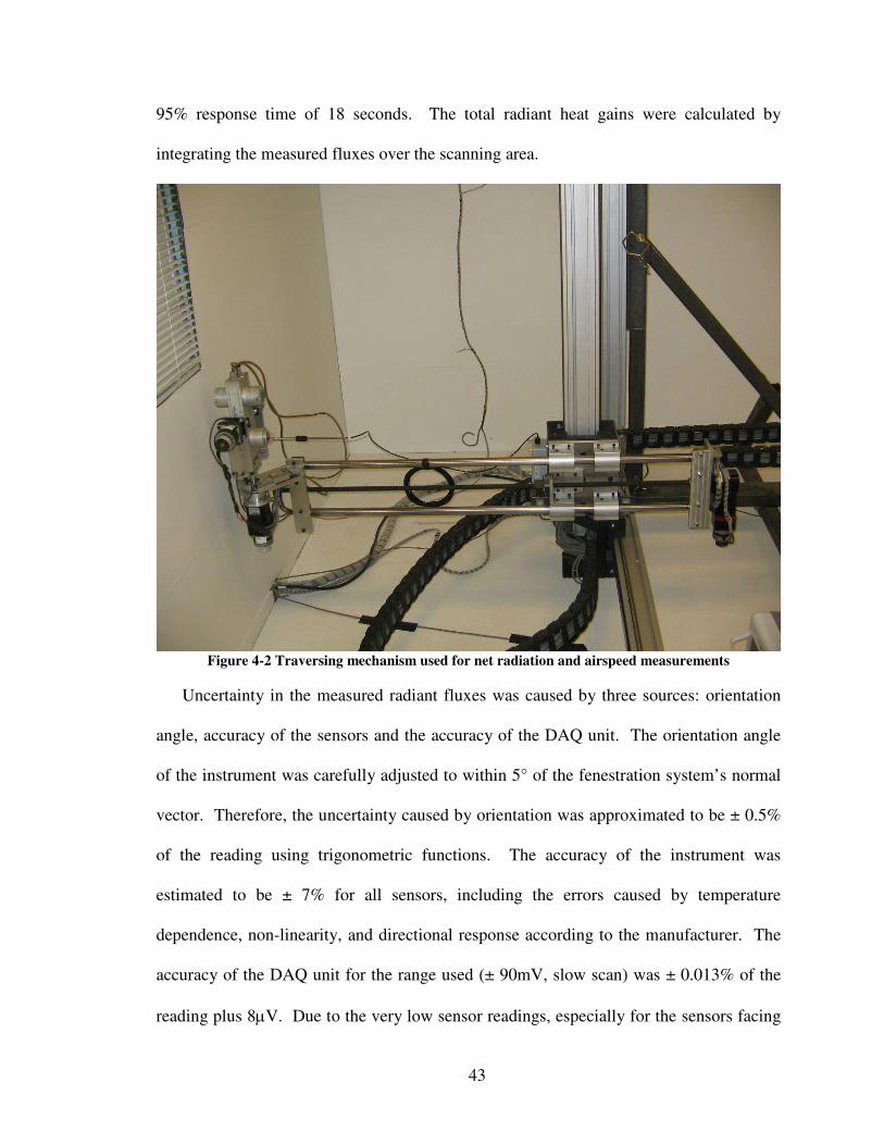
43
95% response time of 18 seconds. The total radiant heat gains were calculated by
integrating the measured fluxes over the scanning area.
Figure 4-2 Traversing mechanism used for net radiation and airspeed measurements
Uncertainty in the measured radiant fluxes was caused by three sources: orientation
angle, accuracy of the sensors and the accuracy of the DAQ unit. The orientation angle
of the instrument was carefully adjusted to within 5° of the fenestration system’s normal
vector. Therefore, the uncertainty caused by orientation was approximated to be ± 0.5%
of the reading using trigonometric functions. The accuracy of the instrument was
estimated to be ± 7% for all sensors, including the errors caused by temperature
dependence, non-linearity, and directional response according to the manufacturer. The
accuracy of the DAQ unit for the range used (± 90mV, slow scan) was ± 0.013% of the
reading plus 8µV. Due to the very low sensor readings, especially for the sensors facing
44
away from the fenestration system, the uncertainty caused by the DAQ unit can be as
high as ± 8.5%.
4.2.5 PressurePressure transducers were used to measure the pressure drop through a flow nozzle in
order to estimate the system flow rate. The transducers used for the current study were
Setra Systems model 264 with a full-scale reading of 0.5 in-H2O (124.5 Pa). The catalog
accuracy of the transducers was ± 1% FS, which was verified with a precision calibration
manometer (±0.0025 in-H2O). The uncertainty of the DAQ unit for the range used (0-
30Vdc slow scan) was ± 0.013% of the reading plus 1.7mV. The uncertainty due to
pressure fluctuations was found to be ± 0.017%. The total uncertainty associated with the
pressure measurements was ± 2.2% for the high flow case and ± 4.3% for the low flow
case.
4.2.6 Airflow SpeedA TSI model 8475-300-1 hot wire anemometer was used to measure the air speed just
in front of the blinds. The hot wire was mounted on the traversing mechanism, which
moved the probe according to a specified grid. The instrument had an adjustable output
type and full-scale range so that higher accuracies could be obtained. An output of 0-
10Vdc was chosen for the current study. The full-scale range was set to 0 to 100 ft/min
(0.51 m/s) for room configuration #1 (Figure 3-5) and 0 to 400 ft/min (2.04 m/s) for room
configuration #2 (Figure 3-6). The instrument had an uncertainty of ± 1% FS or ± 3% of
the reading. Due to the ability to scale the full-scale value, the full-scale uncertainty was
minimized and the uncertainty was approximated as ± 3% of the reading.
45
4.3 Uncertainties in Intermediate VariablesUncertainties in the intermediate variables are discussed in the following sections.
The uncertainties in many of these variables were calculated on a case by case basis and
presented with the final results.
4.3.1 Room Airflow RateThe system volumetric flow rate was measured through two independent flow
measurement chambers as shown in Figure 3-2. These chambers were constructed in
accordance with ANSI/ASHRAE Standard 51-1999 (ASHRAE 1999). A differential
pressure transducer was utilized to measure the pressure drop across an elliptical, 4in
(101.6mm) throat diameter flow nozzle that was placed in the middle of each chamber.
The differential pressure was then used to determine the volumetric flow according to the
procedure given in the standard. The control program only used the data from the
chamber nearest the supply fan, while the other chamber was utilized as a check.
In addition to providing construction procedures, the standard also gives a method for
determining the uncertainty in the measurement as shown in equation 4-15 (ASHRAE
1999).
2
22
22
22 Nf
AcQ uuu
uuu +
+
++= ρ
4-15
Where:
Qu = fractional total uncertainty in airflow rate
cu = fractional uncertainty in nozzle discharge coefficient
Au = fractional uncertainty in nozzle area
46
fu = fractional uncertainty in differential pressure measurement
ρu = fractional uncertainty in air density
Nu = fractional uncertainty caused by variations in the fan speed
The typical values for the uncertainty caused by the nozzle discharge coefficient and
nozzle area were ± 1.2% and ± 0.5%, respectively, as given by the standard (ASHRAE
1999). Fisher (1995) determined that the uncertainty from the air density and fan speed
variation could be estimated at ± 0.1% and 1%, respectively. As discussed in Section
4.2.5, the uncertainty due to the pressure measurements was estimated to be ± 1% FS,
which translated to about ± 2.2% for the high flow (163cfm) case and ± 4.3% for the low
flow (82cfm) case. The final uncertainty for the airflow rate was estimated as ± 2.7%
utilizing equation 4-15.
4.3.2 Heat Extraction RateUncertainties in the air density and specific heat can be assumed negligible according
to Fisher (1995). Therefore, equation 4-3 can be derived using equation 4-14 to form
equation 4-16, which was used to estimate the uncertainty of the room heat extraction
rate. The heat extraction rate was used to determine the heat balance error. The
uncertainties in the temperature difference were determined using equation 4-13 with the
temperature uncertainties discussed in Section 4.2.2.5.
( ) ( )22
extext TQextPq uQuTCu ∆⋅+⋅∆⋅⋅≈ ρ&4-16
Where:
extqu &= uncertainty in heat extraction rate, in [BTU/hr] or [W]
extT∆ = difference between entering and leaving air temperatures, in [°F] or[°C]
47
Q = room volumetric flow rate, in [ft3/hr] or [m3/kg]
Qu = uncertainty in volumetric flow rate, in [ft3/hr] or [m3/kg]
extTu∆ = uncertainty in temperature difference, in [°F] or [°C]
4.3.3 Radiant Heat GainsUncertainty in the net radiant heats gains was introduced from four sources including
propagation of the uncertainty in the measured radiant fluxes, positional offset of the
sensor, the measurement grid density and the error caused by a parallel plane
measurement area. Considering that the traversing mechanism could precisely move the
net-radiometer and the average motor slip was much less than 50 steps (or much less than
0.01in), it was assumed that the uncertainty of the area of measurement was negligible.
Then equation 4-5 can be derived with equation 4-14 to produce equation 4-17, which
was used to determine the uncertainty caused by the propagation of the uncertainty in the
measurement of the radiant fluxes. Estimated uncertainties in the radiant heat gain due to
the propagation of uncertainty in the radiant flux measurements were determined to be
below ± 1.8% for all tests.
( )[ ]∑=
′′⋅≈n
iqiq iradrad
uAu1
2,&
4-17
Where:
radqu & = Uncertainty in net radiant heat gain, in [BTU/hr] or [W]
iradqu,′′ = Uncertainty in net radiant heat flux, in [BTU/hr-ft2] or [W/m2]
Multiple tests were performed to determine the uncertainty due to the measurement
grid density. Five different grid sizes were tested including 1”x1”, 2”x2”, 3”x3”, 4”x4”
and 6”x6” grids with 1476, 378, 168, 81 and 42 data points, respectfully. Figure 4-3
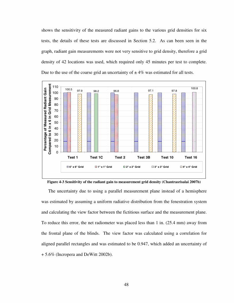
48
shows the sensitivity of the measured radiant gains to the various grid densities for six
tests, the details of these tests are discussed in Section 5.2. As can been seen in the
graph, radiant gain measurements were not very sensitive to grid density, therefore a grid
density of 42 locations was used, which required only 45 minutes per test to complete.
Due to the use of the coarse grid an uncertainty of ± 4% was estimated for all tests.
98.2 96.8100.5 100.897.897.197.9
0
10
20
30
40
50
60
70
80
90
100
110
Test 1 Test 1C Test 2 Test 3B Test 10 Test 16
Per
cen
tag
eof
Mea
sure
dR
adia
nt
Gai
nC
om
pare
dto
6in
x6
inG
rid
Mea
sure
men
t
6" x 6" Grid 1" x 1" Grid 2" x 2" Grid 3" x 3" Grid 4" x 4" Grid
Figure 4-3 Sensitivity of the radiant gain to measurement grid density (Chantrasrisalai 2007b)
The uncertainty due to using a parallel measurement plane instead of a hemisphere
was estimated by assuming a uniform radiative distribution from the fenestration system
and calculating the view factor between the fictitious surface and the measurement plane.
To reduce this error, the net radiometer was placed less than 1 in. (25.4 mm) away from
the frontal plane of the blinds. The view factor was calculated using a correlation for
aligned parallel rectangles and was estimated to be 0.947, which added an uncertainty of
+ 5.6% (Incropera and DeWitt 2002b).
49
4.3.4 Total Fenestration Heat GainThe total fenestration heat gain was simply the sum of the power dissipated by the
window panel and blinds. Since both derivatives of the summing equation were one, the
uncertainty could be expressed as equation 4-18.
22,,, inpblinpwdtotfen qqq uuu &&& += 4-18
Where:
totfenqu,&
= uncertainty in total fenestration heat gain, in [BTU/hr] or [W]
inpwdqu,&
= uncertainty in window panel power dissipation, in [BTU/hr] or [W]
inpblqu,&
= uncertainty in blind power dissipation, in [BTU/hr] or [W]
4.3.5 Convective Heat GainThe convective heat gain into the test room was calculated with the dimensional form
of equation 4-7. With this equation along with equation 4-14, the uncertainty calculation
became equation 4-19.
22,,, radfentotfenconvfen qqq uuu &&& += 4-19
Where:
convfenqu,& = uncertainty in the convective heat gain, in [BTU/hr] or [W]
radfenqu,&
= uncertainty in radiant heat gain from the fenestration system, note this
is not equal toradqu & , in [BTU/hr] or [W]
4.3.6 Fictitious Fenestration Surface TemperatureThe uncertainty in the fictitious surface temperature is produced from three sources
including the uncertainty in the net radiant heat gain, room surface temperatures and
50
emissivities of the room surfaces. The uncertainty from these three sources can be
combined with equation 4-13 to form equation 4-20 (Chantrasrisalai 2007b).
2221 εuuuu TqT ++= &
4-20
Where:
1Tu = uncertainty in the fictitious fenestration surface temperature, in [°F]
or [°C]
qu & = uncertainty in 1T due to the uncertainty in the net radiant heat gain, in
[°F] or [°C]
Tu = uncertainty in 1T due to the uncertainty in the room surface
temperatures, in [°F] or [°C]
εu = uncertainty in 1T due to the uncertainty in the room surface
emissivities, in [°F] or [°C]
Uncertainty due to the propagation of the uncertainty in the net radiant heat gain can
be estimated with equation 4-21.
)()(,,1,1 radfenqradfenradfenq uqTqTu && && ±±= 4-21
Uncertainty due to the propagation of the uncertainty in the room surface
temperatures was estimated with equation 4-22.
222 ...32 nTTTTTTT uuuu +++= 4-22
Where:
nTTu = uncertainty of the surface temperature of each room surface, in [°F]
or [°C]
And:
51
)()( 11 jj TjjTT uTTTTu ±±= 4-23
Where j was from 2 to the number of room surfaces.
Uncertainty due to the propagation of the uncertainty in the surface emissivities could
be estimated with equation 4-24, but it was determined that equation 4-24 was
approximately equal to the propagation of the uncertainty in the emissivity of just the
fictitious fenestration surface.
121
222 ... εεεεε TTTT uuuuun≈+++= 4-24
Where:
1εTu = uncertainty due to the propagation of the uncertainty of the emissivity
of the fictitious surface, in [°F] or [°C]
And:
)()(11 1111 εε εε uTTuT ±±= 4-25
Where:
1εu = uncertainty in the emissivity of the fictitious surface (approximately ±
0.05)
4.4 Propagation of Uncertainty Analysis to Results
4.4.1 Radiative/Convective SplitThe uncertainty for the radiative fraction can be found by combining equations 4-6
and 4-14, resulting in equation 4-26. The convective fraction was calculated with
equation 4-7, which when combined with equation 4-14 reduces to equation 4-27.
( ) ( )2,2
,2,
,,,
1totfenradfenradfen qradfenqtotfen
totfenF uquq
qu && &&
&⋅+⋅⋅=
4-26
52
radfenconvfen FF uu,,
= 4-27
Where:
radfenFu,
= uncertainty in the radiative fraction
convfenFu,
= uncertainty in the convective fraction
4.4.2 Convection CoefficientThe uncertainty in the fictitious surface convection coefficient was estimated by
combining equations 4-11 and 4-14, resulting in equation 4-28.
( ) ( )2,2
21
,,
1reffenconvfeninc Tconvfenqreffen
reffenh uquT
TAu
−∆−−
⋅+⋅∆⋅∆⋅
= &&
4-28
Where:
reffenT −∆ = difference between fictitious surface temperature and the reference
temperature, in [°F] or [°C]
And:
221 refreffen TTT uuu +=
−∆4-29
4.4.3 Thermal ConductanceThe uncertainty in the thermal conductance of the fictitious layer was estimated by
combining equations 4-12 and 4-14, resulting in equation 4-30.
( ) ( )2,2
21
,1
1wdfeninpwdL Tinpwdqwdfen
wdfenC uquT
TAu
−+ ∆−−
⋅+⋅∆⋅∆⋅
= &&
4-30
Where:
wdfenT −∆ = difference between fictitious surface temperature and the temperature
of the window panel, in [°F] or [°C]
And:
53
221 wdwdfen TTT uuu +=
−∆4-31
4.5 Validation of Experimental FacilityThe results of an experimental study can only be as trustworthy as the experimental
facility utilized. Therefore, the reliability and accuracy of the facility was examined in
detail. Although a heat balance was not necessary for the proposed experimental method,
it was instantaneously calculated throughout each experimental test. The heat balance
was monitored as an indicator of steady-steady conditions as described in Section 5.1.
The heat balance error ranged between 5 and 14% for room configuration #1 (Figure
3-5), which featured an unducted return. When a ducted return was installed for room
configuration #2 (Figure 3-6), the heat balance error ranged between 0.5 and 5%. The
discrepancy occurred due to air leakage into the ceiling plenum from the guard space
resulting in an unbalanced system. Once at steady-state, the facility was able to tightly
hold a constant heat balance error, room temperature and guard space temperature.
The most critical measurement for the current study was the net radiant heat gain
from the fenestration system. This parameter allowed radiant/convective splits, fictitious
fenestration surface temperature and convection coefficients to be calculated. The radiant
heat gain was calculated utilizing heat flux data measured by the net radiometer.
Before testing began on the complex fenestration system, only the window panel was
installed in the laboratory. Radiation heat transfer measurements from the panel were
available and were compared to theoretical calculations. Figure 4-4 shows the measured
versus calculated radiant heat transfer from the panel to the room, while Figure 4-5 shows
the measured panel temperature versus calculated panel temperature (Chantrasrisalai
2007a). The figures demonstrate that the measurements were very close to calculated

54
values and were well within the associated uncertainty. These graphs not only validated
the heat flux measurements but also the window panel and room surface temperature
measurements and the calculated surface view factors.
0
50
100
150
200
250
300
350
400
450
500
550
0 50 100 150 200 250 300 350 400 450 500 550
Measured Radiant Gain, Btu/hr
Cal
cula
ted
Rad
ian
tG
ain
,Btu
/hr
Figure 4-4 Validation of measured radiant heat gain (Chantrasrisalai 2007a)
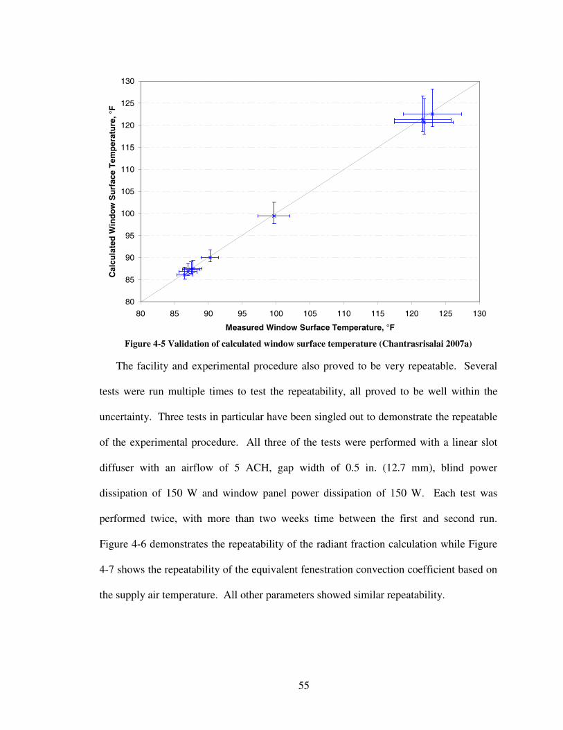
55
80
85
90
95
100
105
110
115
120
125
130
80 85 90 95 100 105 110 115 120 125 130
Measured Window Surface Temperature, °F
Cal
cula
ted
Win
do
wS
urf
ace
Tem
per
atu
re,°
F
Figure 4-5 Validation of calculated window surface temperature (Chantrasrisalai 2007a)
The facility and experimental procedure also proved to be very repeatable. Several
tests were run multiple times to test the repeatability, all proved to be well within the
uncertainty. Three tests in particular have been singled out to demonstrate the repeatable
of the experimental procedure. All three of the tests were performed with a linear slot
diffuser with an airflow of 5 ACH, gap width of 0.5 in. (12.7 mm), blind power
dissipation of 150 W and window panel power dissipation of 150 W. Each test was
performed twice, with more than two weeks time between the first and second run.
Figure 4-6 demonstrates the repeatability of the radiant fraction calculation while Figure
4-7 shows the repeatability of the equivalent fenestration convection coefficient based on
the supply air temperature. All other parameters showed similar repeatability.
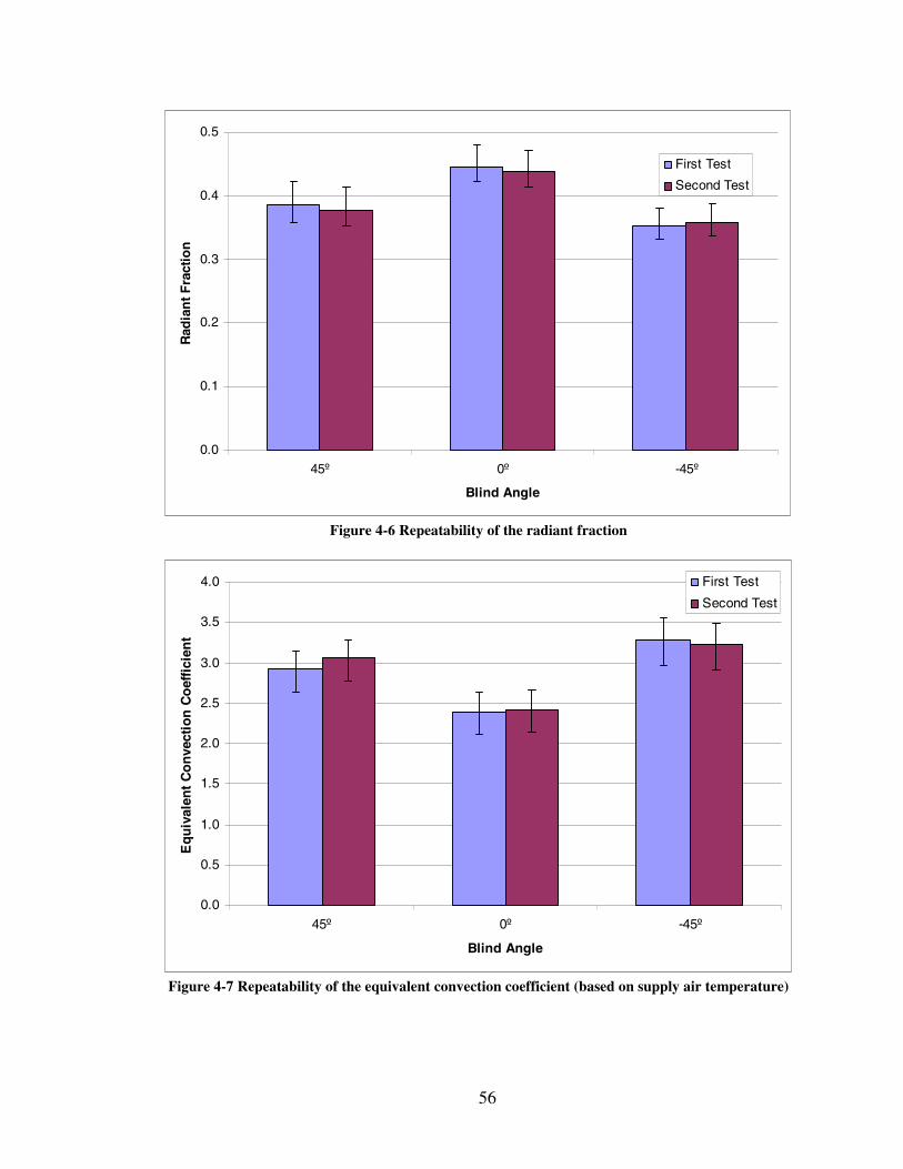
56
0.0
0.1
0.2
0.3
0.4
0.5
45º 0º -45º
Blind Angle
Rad
ian
tF
ract
ion
First Test
Second Test
Figure 4-6 Repeatability of the radiant fraction
0.0
0.5
1.0
1.5
2.0
2.5
3.0
3.5
4.0
45º 0º -45º
Blind Angle
Eq
uiv
alen
tC
on
vect
ion
Co
effi
cien
t
First Test
Second Test
Figure 4-7 Repeatability of the equivalent convection coefficient (based on supply air temperature)
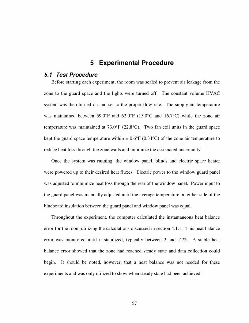
57
5 Experimental Procedure
5.1 Test ProcedureBefore starting each experiment, the room was sealed to prevent air leakage from the
zone to the guard space and the lights were turned off. The constant volume HVAC
system was then turned on and set to the proper flow rate. The supply air temperature
was maintained between 59.0°F and 62.0°F (15.0°C and 16.7°C) while the zone air
temperature was maintained at 73.0°F (22.8°C). Two fan coil units in the guard space
kept the guard space temperature within ± 0.6°F (0.34°C) of the zone air temperature to
reduce heat loss through the zone walls and minimize the associated uncertainty.
Once the system was running, the window panel, blinds and electric space heater
were powered up to their desired heat fluxes. Electric power to the window guard panel
was adjusted to minimize heat loss through the rear of the window panel. Power input to
the guard panel was manually adjusted until the average temperature on either side of the
blueboard insulation between the guard panel and window panel was equal.
Throughout the experiment, the computer calculated the instantaneous heat balance
error for the room utilizing the calculations discussed in section 4.1.1. This heat balance
error was monitored until it stabilized, typically between 2 and 12%. A stable heat
balance error showed that the zone had reached steady state and data collection could
begin. It should be noted, however, that a heat balance was not needed for these
experiments and was only utilized to show when steady state had been achieved.
58
Once the zone had achieved steady state, data collection began. Surface temperature
data was recorded while the net radiometer traversed its measurement plane as described
in Section 4.2.4. Two sets of radiation data were collected for each experiment; each
requiring roughly 45 minutes to complete. Each experiment required roughly six hours to
run, including the time required to reach steady-state.
Once one experiment had finished, the system was left running while various
experimental parameters were reconfigured. To save time and materials, experiments
were performed in an order that required minimal entry into the test room. The only
parameters that required entry into the room to change were blind slat angel, window-
blind gap width and the supply/return diffuser configurations.
Twelve zero airflow tests were also preformed, which required a slightly modified
testing procedure. First, all testing parameters were setup as if the most similar high flow
test was to occur. After the test room had reached steady-state for an acceptable period
of time (typically three hours), the supply fan and plug load were turned off. The room
was then allowed to reach a quasi-steady-state condition, where the fenestration and
surface temperatures had stabilized. Quasi steady-state conditions were typically
achieved after two hours. After two hours had elapsed, heat balance data recording was
started and two sets of radiation measurements were performed. In order to save time,
zero airflow tests were typically performed immediately following the most similar high
flow test.
The appendixes provide a more detailed description of the day-to-day operation of the
facility and HVAC system. Appendix A contained detailed procedures for running the
59
system, control program, instrumentation and experiments. Appendix C provides
trouble-shooting procedures for many possible problems.
5.2 Parametric Simulation SetThe current study produced results for a limited number and range of parameters.
The parametric set of experiments is outlined in Table 5-1. A total of 52 experiments
were performed not including the verification tests, which are detailed in Chapter 4.5 and
a handful of sensitivity tests. Variable parameters for the current study included blind
angle, gap width between the blind and window panel, room airflow rate, room
configuration and the blind and window panel heat flux. The plug load was set so that
the room would achieve a temperature of 73°F (22.8°C) with a supply temperature of
61°F (16.1°C) for all experiments. Two room diffuser configurations were tested;
configuration number one refers to Figure 3-5 while configuration number two refers to
Figure 3-6.

60
Table 5-1 Parameters for the 52 experimentsSlat Angle Gap Width Airflow
° [in] (mm) Watts Watts cfm Watts1 150 150 163 331 #12 150 50 163 431 #13 50 150 163 431 #14 50 50 163 531 #15 150 150 82 16 #16 150 50 82 116 #17 50 150 82 116 #18 50 50 82 216 #19 150 150 163 331 #110 150 50 163 431 #111 50 150 163 431 #112 50 50 163 531 #115 50 150 82 116 #116 50 50 82 216 #117 150 150 163 331 #118 150 50 163 431 #119 50 150 163 431 #120 50 50 163 531 #123 50 150 82 116 #124 50 50 82 216 #125 150 150 0 0 #126 50 50 0 0 #127 150 150 0 0 #128 50 50 0 0 #129 150 150 0 0 #130 50 50 0 0 #131 150 150 163 331 #132 50 50 163 531 #133 0 150 150 0 0 #134 150 150 163 331 #135 50 50 163 531 #136 0 150 150 0 0 #137 150 150 163 331 #138 50 50 163 531 #139 0 150 150 0 0 #140 150 150 163 331 #141 50 50 163 531 #142 0 150 150 0 0 #143 150 150 163 331 #144 50 50 163 531 #145 0 150 150 0 0 #146 150 150 163 331 #147 50 50 163 531 #148 0 150 150 0 0 #149 10 150 150 163 331 #251 5 150 150 82 16 #253 10 150 150 163 331 #255 5 150 150 82 16 #257 10 150 150 163 331 #259 5 150 150 82 16 #261 1.75 (44.5) 150 150 163 331 #262 3.75 (95.25) 150 150 163 331 #2
0 10
0.5 (12.7)
45 10
-45 10
0
45
45
0 10
10
-45
Window Power Blind PowerACH
1.75 (44.5)
0
-4510
0
0
Plug Load
45
5
10
5
10
Test No.
-45
RoomConfiguration
0 10
3.75 (95.25)45 10
-45
5
Figure 5-1 illustrates the three different gap widths that were tests for the current
project. As shown in the figures the blinds were never moved and their frontal plane (at a
slat angle of 0°) was located on the frontal plane of the partition wall. It should also be
noted that the gap-width for the current work was defined as the distance between the
window surface and the back plane of the blinds at a slat angle of 0°, therefore the gap
actually increased slightly when the slats were placed at an angle which was analogous to
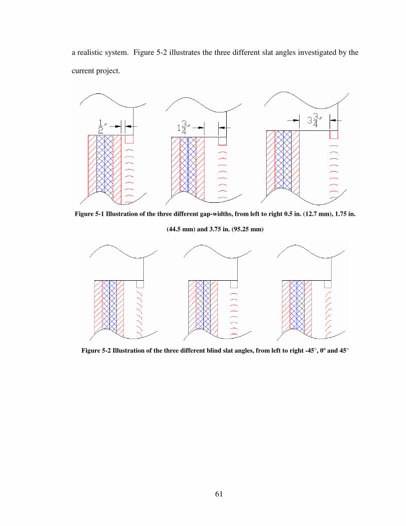
61
a realistic system. Figure 5-2 illustrates the three different slat angles investigated by the
current project.
Figure 5-1 Illustration of the three different gap-widths, from left to right 0.5 in. (12.7 mm), 1.75 in.
(44.5 mm) and 3.75 in. (95.25 mm)
Figure 5-2 Illustration of the three different blind slat angles, from left to right -45°, 0º and 45°
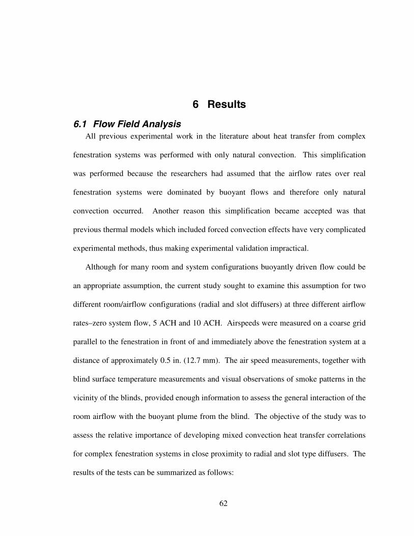
62
6 Results
6.1 Flow Field AnalysisAll previous experimental work in the literature about heat transfer from complex
fenestration systems was performed with only natural convection. This simplification
was performed because the researchers had assumed that the airflow rates over real
fenestration systems were dominated by buoyant flows and therefore only natural
convection occurred. Another reason this simplification became accepted was that
previous thermal models which included forced convection effects have very complicated
experimental methods, thus making experimental validation impractical.
Although for many room and system configurations buoyantly driven flow could be
an appropriate assumption, the current study sought to examine this assumption for two
different room/airflow configurations (radial and slot diffusers) at three different airflow
rates–zero system flow, 5 ACH and 10 ACH. Airspeeds were measured on a coarse grid
parallel to the fenestration in front of and immediately above the fenestration system at a
distance of approximately 0.5 in. (12.7 mm). The air speed measurements, together with
blind surface temperature measurements and visual observations of smoke patterns in the
vicinity of the blinds, provided enough information to assess the general interaction of the
room airflow with the buoyant plume from the blind. The objective of the study was to
assess the relative importance of developing mixed convection heat transfer correlations
for complex fenestration systems in close proximity to radial and slot type diffusers. The
results of the tests can be summarized as follows:
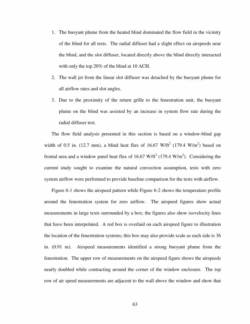
63
1. The buoyant plume from the heated blind dominated the flow field in the vicinity
of the blind for all tests. The radial diffuser had a slight effect on airspeeds near
the blind, and the slot diffuser, located directly above the blind directly interacted
with only the top 20% of the blind at 10 ACH.
2. The wall jet from the linear slot diffuser was detached by the buoyant plume for
all airflow rates and slot angles.
3. Due to the proximity of the return grille to the fenestration unit, the buoyant
plume on the blind was assisted by an increase in system flow rate during the
radial diffuser test.
The flow field analysis presented in this section is based on a window-blind gap
width of 0.5 in. (12.7 mm), a blind heat flux of 16.67 W/ft2 (179.4 W/m2) based on
frontal area and a window panel heat flux of 16.67 W/ft2 (179.4 W/m2). Considering the
current study sought to examine the natural convection assumption, tests with zero
system airflow were performed to provide baseline comparison for the tests with airflow.
Figure 6-1 shows the airspeed pattern while Figure 6-2 shows the temperature profile
around the fenestration system for zero airflow. The airspeed figures show actual
measurements in large texts surrounded by a box; the figures also show isovelocity lines
that have been interpolated. A red box is overlaid on each airspeed figure to illustration
the location of the fenestration systems; this box may also provide scale as each side is 36
in. (0.91 m). Airspeed measurements identified a strong buoyant plume from the
fenestration. The upper row of measurements on the airspeed figure shows the airspeeds
nearly doubled while contracting around the corner of the window enclosure. The top
row of air speed measurements are adjacent to the wall above the window and show that
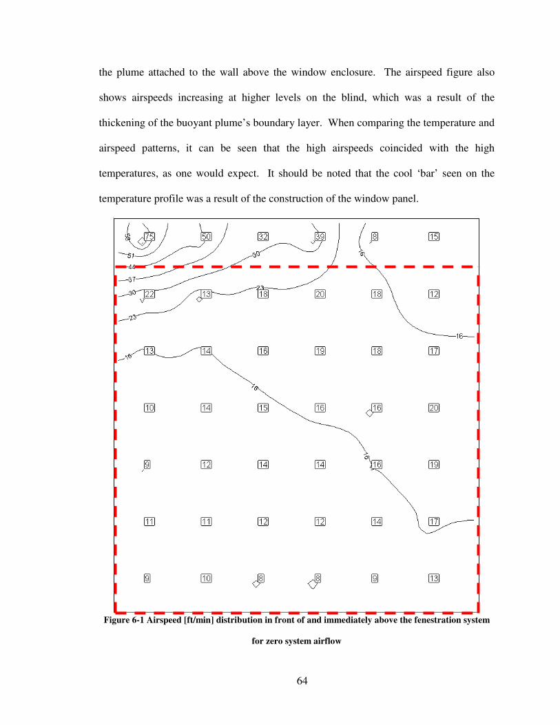
64
the plume attached to the wall above the window enclosure. The airspeed figure also
shows airspeeds increasing at higher levels on the blind, which was a result of the
thickening of the buoyant plume’s boundary layer. When comparing the temperature and
airspeed patterns, it can be seen that the high airspeeds coincided with the high
temperatures, as one would expect. It should be noted that the cool ‘bar’ seen on the
temperature profile was a result of the construction of the window panel.
Figure 6-1 Airspeed [ft/min] distribution in front of and immediately above the fenestration system
for zero system airflow
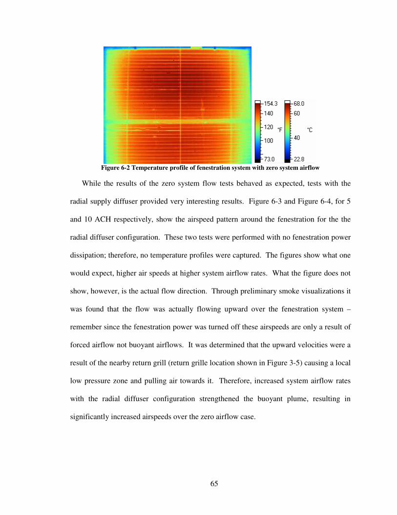
65
Figure 6-2 Temperature profile of fenestration system with zero system airflow
While the results of the zero system flow tests behaved as expected, tests with the
radial supply diffuser provided very interesting results. Figure 6-3 and Figure 6-4, for 5
and 10 ACH respectively, show the airspeed pattern around the fenestration for the the
radial diffuser configuration. These two tests were performed with no fenestration power
dissipation; therefore, no temperature profiles were captured. The figures show what one
would expect, higher air speeds at higher system airflow rates. What the figure does not
show, however, is the actual flow direction. Through preliminary smoke visualizations it
was found that the flow was actually flowing upward over the fenestration system –
remember since the fenestration power was turned off these airspeeds are only a result of
forced airflow not buoyant airflows. It was determined that the upward velocities were a
result of the nearby return grill (return grille location shown in Figure 3-5) causing a local
low pressure zone and pulling air towards it. Therefore, increased system airflow rates
with the radial diffuser configuration strengthened the buoyant plume, resulting in
significantly increased airspeeds over the zero airflow case.
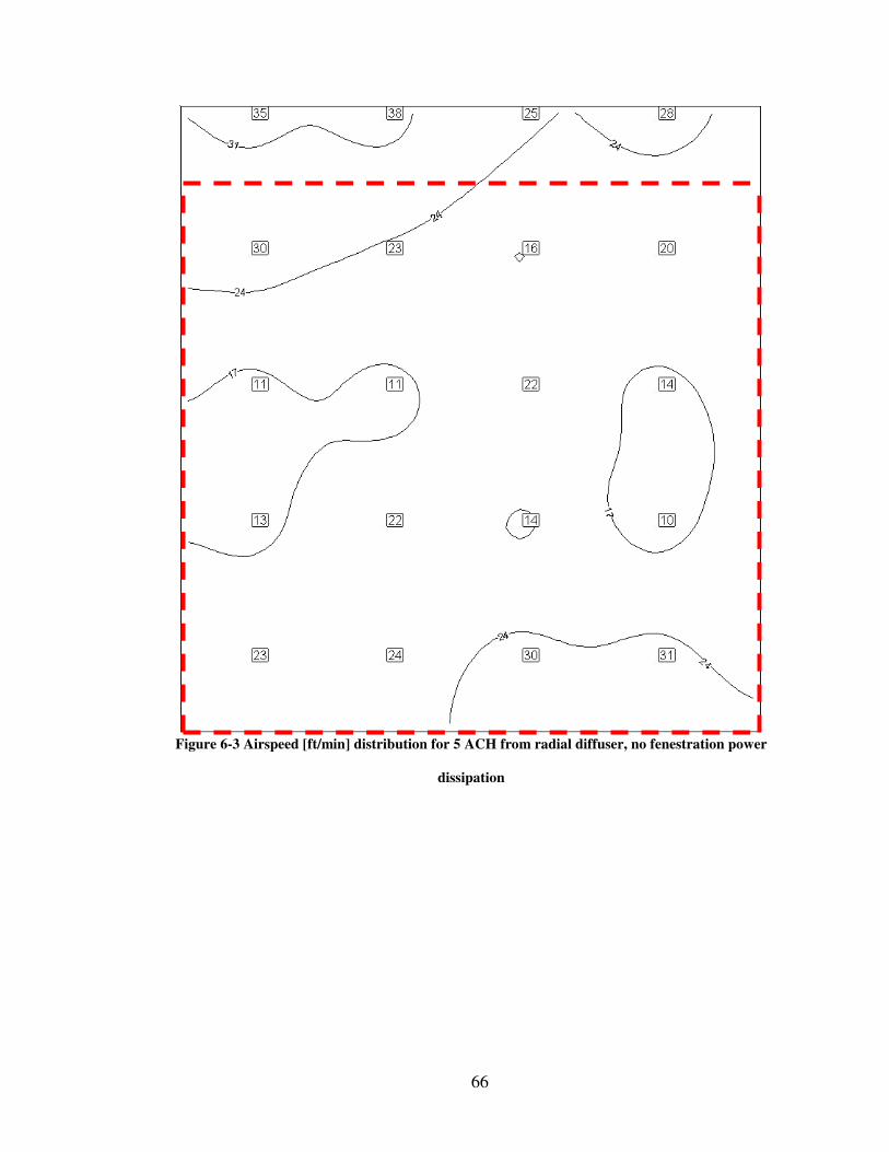
66
Figure 6-3 Airspeed [ft/min] distribution for 5 ACH from radial diffuser, no fenestration power
dissipation
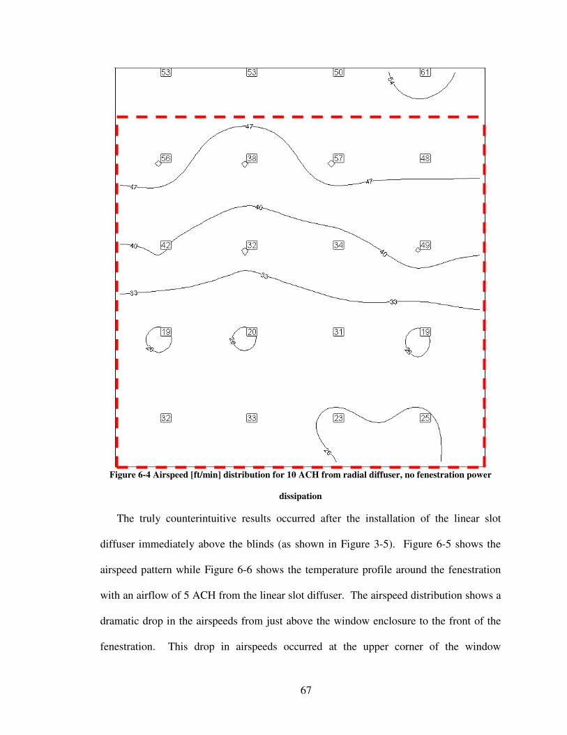
67
Figure 6-4 Airspeed [ft/min] distribution for 10 ACH from radial diffuser, no fenestration power
dissipation
The truly counterintuitive results occurred after the installation of the linear slot
diffuser immediately above the blinds (as shown in Figure 3-5). Figure 6-5 shows the
airspeed pattern while Figure 6-6 shows the temperature profile around the fenestration
with an airflow of 5 ACH from the linear slot diffuser. The airspeed distribution shows a
dramatic drop in the airspeeds from just above the window enclosure to the front of the
fenestration. This drop in airspeeds occurred at the upper corner of the window
68
enclosure. Although the average airspeed just above the fenestration was nearly 150
ft/min (0.76 m/s), the airspeed in front of the blind was very similar to the zero airflow
tests. The temperature profile also showed a negligible difference from the zero airflow
case (Figure 6-2), indicating a similar airflow pattern. These two figures show that the
wall jet was separating at the corner of the enclosure. Preliminary smoke tests confirmed
the wall jet separation and indicated that the buoyant plume was fully present over the
fenestration itself. The wall jet and buoyant plume combined at the separation point,
resulting in very turbulent mixed airflow.
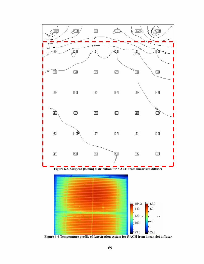
69
Figure 6-5 Airspeed [ft/min] distribution for 5 ACH from linear slot diffuser
Figure 6-6 Temperature profile of fenestration system for 5 ACH from linear slot diffuser
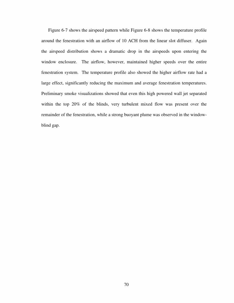
70
Figure 6-7 shows the airspeed pattern while Figure 6-8 shows the temperature profile
around the fenestration with an airflow of 10 ACH from the linear slot diffuser. Again
the airspeed distribution shows a dramatic drop in the airspeeds upon entering the
window enclosure. The airflow, however, maintained higher speeds over the entire
fenestration system. The temperature profile also showed the higher airflow rate had a
large effect, significantly reducing the maximum and average fenestration temperatures.
Preliminary smoke visualizations showed that even this high powered wall jet separated
within the top 20% of the blinds, very turbulent mixed flow was present over the
remainder of the fenestration, while a strong buoyant plume was observed in the window-
blind gap.
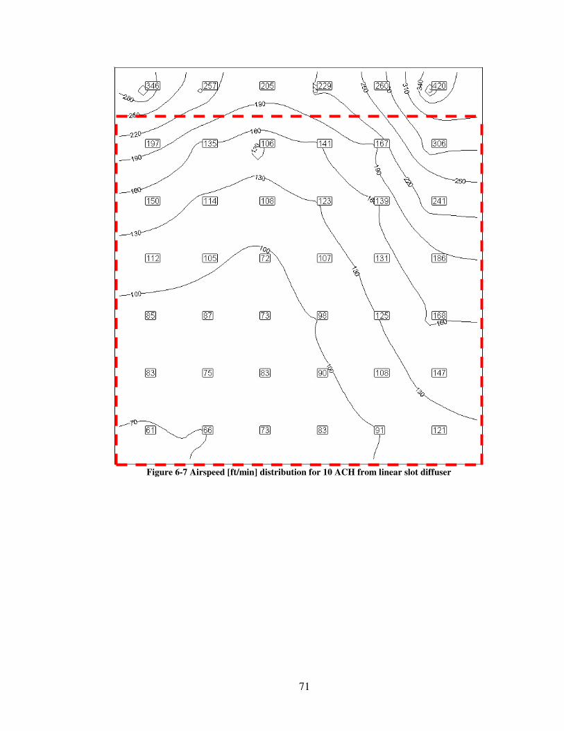
71
Figure 6-7 Airspeed [ft/min] distribution for 10 ACH from linear slot diffuser
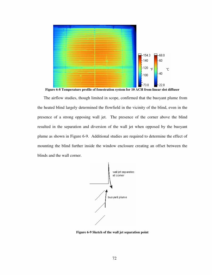
72
Figure 6-8 Temperature profile of fenestration system for 10 ACH from linear slot diffuser
The airflow studies, though limited in scope, confirmed that the buoyant plume from
the heated blind largely determined the flowfield in the vicinity of the blind, even in the
presence of a strong opposing wall jet. The presence of the corner above the blind
resulted in the separation and diversion of the wall jet when opposed by the buoyant
plume as shown in Figure 6-9. Additional studies are required to determine the effect of
mounting the blind further inside the window enclosure creating an offset between the
blinds and the wall corner.
Figure 6-9 Sketch of the wall jet separation point
73
6.2 Heat Transfer AnalysisThe airflow analysis indicated that convective heat transfer from the fenestration
system will be characterized by natural and mixed convection. As with the airflow
analysis, heat transfer tests were performed with two different room/airflow
configurations (radial and slot diffusers) at three different airflow rates–zero system flow,
5 ACH and 10 ACH. Tests also were conducted with three different blind angles, -45°,
0° and 45°, and three different gap widths, 0.5 in. (12.7 mm), 1.75 in. (44.5 mm) and 3.75
in. (95.3 mm) and four combinations of blind/window electric heating power levels. The
radiation heat flux for the fenestration system was found using a scanning net radiometer,
which was then integrated to find the total radiation heat gain from the fenestration. The
radiative fraction was then calculated by simply subtracting the radiation heat gain from
the total fenestration heat gain, which was measured with precision power transducers.
Table 6-1 shows the total fenestration radiant fraction of each test performed, not
including sensitivity and validation tests, as well as the specific test parameters.
Figure 6-10 shows the affect of window-blind gap width, power dissipation and blind
slot angle. All 18 of the tests present in the figure were conducted with the radial supply
diffuser with an airflow rate of 10 ACH. The plot shows a discernible correlation
between radiative fraction and window-blind gap width, though many of the differences
between data points are within the margin of uncertainty. Window blind gap-width was
also identified as a significant parameter in the literature (Machin et al. 1998; Duarte et
al. 2001), although the previous studies did not examine the larger gaps. The plot also
shows higher radiative fractions for low power on the blind. For this data, the high
uncertainty interval coupled with the consistency of the data indicates that the random
error is likely lower than indicated by the uncertainty intervals. Reduction of the
74
systematic data by calibration of the power measurement is required in order to analyze
this data further.
Figure 6-11 shows the effect of different power dissipation combinations, blind slat
angles and system airflow rate on the radiant fraction of the combined fenestration
system. All tests shown in the figure were completed with the radial supply diffuser.
The most notable point is that for the +- 45° case, there is no measurable difference
between the power input level and the radiative fraction. The only measurable effect is
between 'blinds open' and 'blinds closed' for the high power window case. For a hot
window the position of the blind (open or closed) has a significant effect on the radiative
fraction, otherwise it does not.
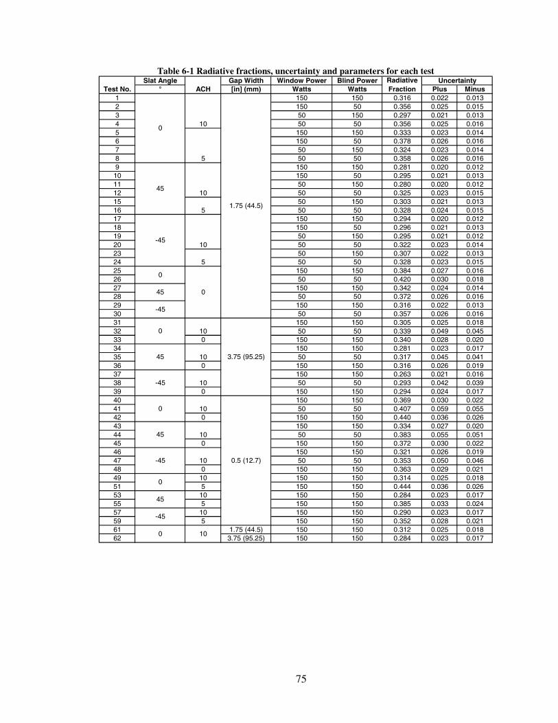
75
Table 6-1 Radiative fractions, uncertainty and parameters for each testSlat Angle Gap Width Window Power Blind Power
° [in] (mm) Watts Watts Plus Minus1 150 150 0.316 0.022 0.0132 150 50 0.356 0.025 0.0153 50 150 0.297 0.021 0.0134 50 50 0.356 0.025 0.0165 150 150 0.333 0.023 0.0146 150 50 0.378 0.026 0.0167 50 150 0.324 0.023 0.0148 50 50 0.358 0.026 0.0169 150 150 0.281 0.020 0.01210 150 50 0.295 0.021 0.01311 50 150 0.280 0.020 0.01212 50 50 0.325 0.023 0.01515 50 150 0.303 0.021 0.01316 50 50 0.328 0.024 0.01517 150 150 0.294 0.020 0.01218 150 50 0.296 0.021 0.01319 50 150 0.295 0.021 0.01220 50 50 0.322 0.023 0.01423 50 150 0.307 0.022 0.01324 50 50 0.328 0.023 0.01525 150 150 0.384 0.027 0.01626 50 50 0.420 0.030 0.01827 150 150 0.342 0.024 0.01428 50 50 0.372 0.026 0.01629 150 150 0.316 0.022 0.01330 50 50 0.357 0.026 0.01631 150 150 0.305 0.025 0.01832 50 50 0.339 0.049 0.04533 0 150 150 0.340 0.028 0.02034 150 150 0.281 0.023 0.01735 50 50 0.317 0.045 0.04136 0 150 150 0.316 0.026 0.01937 150 150 0.263 0.021 0.01638 50 50 0.293 0.042 0.03939 0 150 150 0.294 0.024 0.01740 150 150 0.369 0.030 0.02241 50 50 0.407 0.059 0.05542 0 150 150 0.440 0.036 0.02643 150 150 0.334 0.027 0.02044 50 50 0.383 0.055 0.05145 0 150 150 0.372 0.030 0.02246 150 150 0.321 0.026 0.01947 50 50 0.353 0.050 0.04648 0 150 150 0.363 0.029 0.02149 10 150 150 0.314 0.025 0.01851 5 150 150 0.444 0.036 0.02653 10 150 150 0.284 0.023 0.01755 5 150 150 0.385 0.033 0.02457 10 150 150 0.290 0.023 0.01759 5 150 150 0.352 0.028 0.02161 1.75 (44.5) 150 150 0.312 0.025 0.01862 3.75 (95.25) 150 150 0.284 0.023 0.017
10
RadiativeFraction
Uncertainty
45 10
-45 10 0.5 (12.7)
-45
45
0
-45
0
10
0 10
3.75 (95.25)45 10
0 10
45
010
5
10
Test No.
0
45
10
5
-45
0
1.75 (44.5)
ACH
-45
5
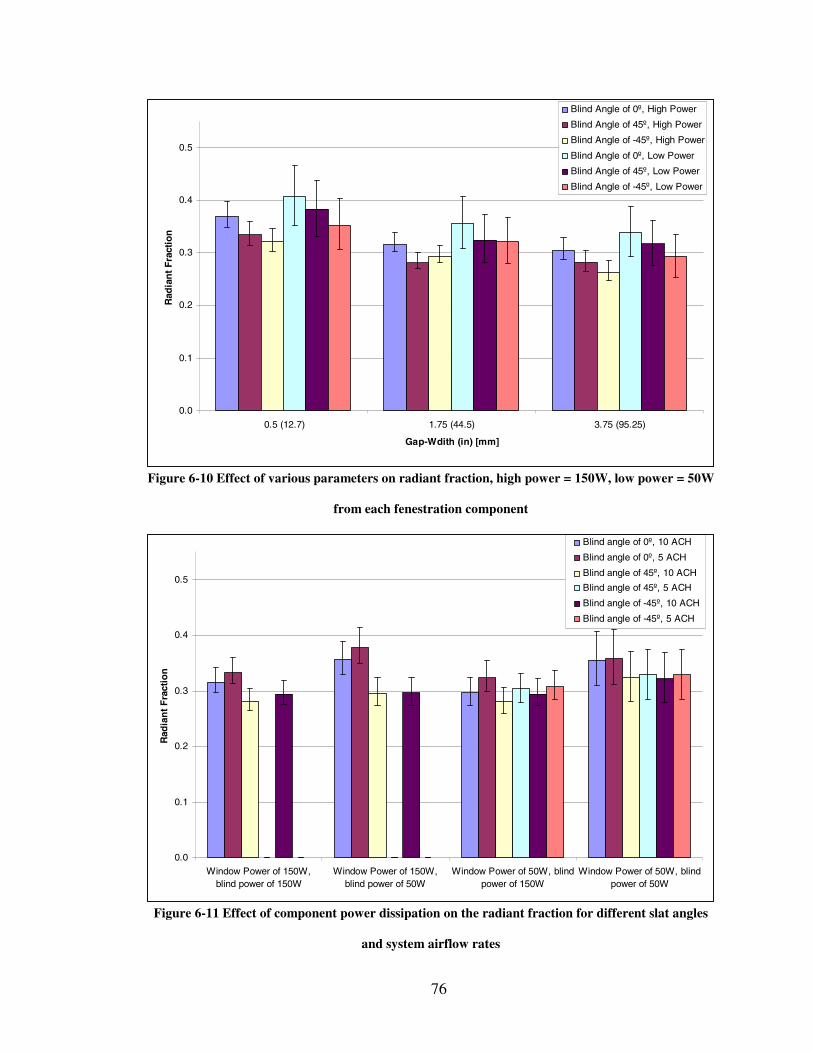
76
0.0
0.1
0.2
0.3
0.4
0.5
0.5 (12.7) 1.75 (44.5) 3.75 (95.25)
Gap-Wdith (in) [mm]
Rad
ian
tF
ract
ion
Blind Angle of 0º, High Power
Blind Angle of 45º, High Power
Blind Angle of -45º, High Power
Blind Angle of 0º, Low Power
Blind Angle of 45º, Low Power
Blind Angle of -45º, Low Power
Figure 6-10 Effect of various parameters on radiant fraction, high power = 150W, low power = 50W
from each fenestration component
0.0
0.1
0.2
0.3
0.4
0.5
Window Power of 150W,blind power of 150W
Window Power of 150W,blind power of 50W
Window Power of 50W, blindpower of 150W
Window Power of 50W, blindpower of 50W
Rad
ian
tF
ract
ion
Blind angle of 0º, 10 ACH
Blind angle of 0º, 5 ACH
Blind angle of 45º, 10 ACH
Blind angle of 45º, 5 ACH
Blind angle of -45º, 10 ACH
Blind angle of -45º, 5 ACH
Figure 6-11 Effect of component power dissipation on the radiant fraction for different slat angles
and system airflow rates
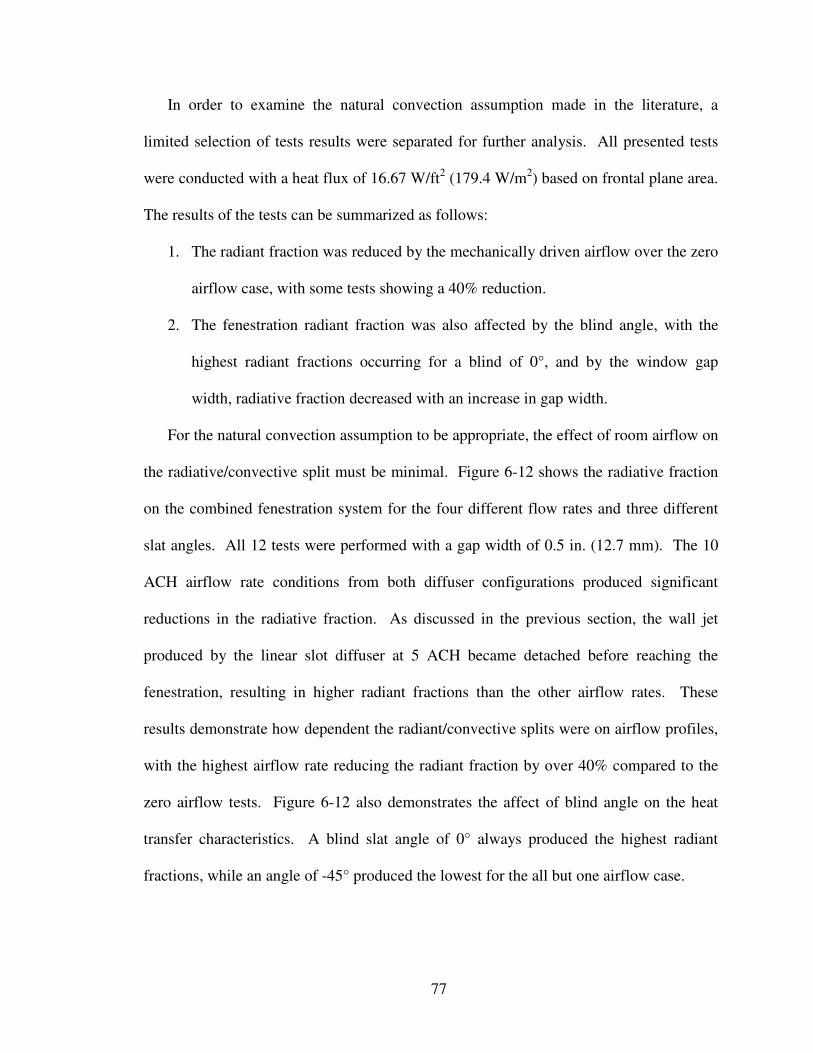
77
In order to examine the natural convection assumption made in the literature, a
limited selection of tests results were separated for further analysis. All presented tests
were conducted with a heat flux of 16.67 W/ft2 (179.4 W/m2) based on frontal plane area.
The results of the tests can be summarized as follows:
1. The radiant fraction was reduced by the mechanically driven airflow over the zero
airflow case, with some tests showing a 40% reduction.
2. The fenestration radiant fraction was also affected by the blind angle, with the
highest radiant fractions occurring for a blind of 0°, and by the window gap
width, radiative fraction decreased with an increase in gap width.
For the natural convection assumption to be appropriate, the effect of room airflow on
the radiative/convective split must be minimal. Figure 6-12 shows the radiative fraction
on the combined fenestration system for the four different flow rates and three different
slat angles. All 12 tests were performed with a gap width of 0.5 in. (12.7 mm). The 10
ACH airflow rate conditions from both diffuser configurations produced significant
reductions in the radiative fraction. As discussed in the previous section, the wall jet
produced by the linear slot diffuser at 5 ACH became detached before reaching the
fenestration, resulting in higher radiant fractions than the other airflow rates. These
results demonstrate how dependent the radiant/convective splits were on airflow profiles,
with the highest airflow rate reducing the radiant fraction by over 40% compared to the
zero airflow tests. Figure 6-12 also demonstrates the affect of blind angle on the heat
transfer characteristics. A blind slat angle of 0° always produced the highest radiant
fractions, while an angle of -45° produced the lowest for the all but one airflow case.
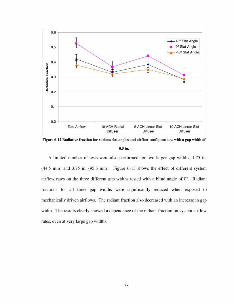
78
0.0
0.1
0.2
0.3
0.4
0.5
0.6
Zero Airflow 10 ACH RadialDiffuser
5 ACH Linear SlotDiffuser
10 ACH Linear SlotDiffuser
Rad
iati
veF
ract
ion
45º Slat Angle
0º Slat Angle
-45º Slat Angle
Figure 6-12 Radiative fraction for various slat angles and airflow configurations with a gap width of
0.5 in.
A limited number of tests were also performed for two larger gap widths, 1.75 in.
(44.5 mm) and 3.75 in. (95.3 mm). Figure 6-13 shows the effect of different system
airflow rates on the three different gap widths tested with a blind angle of 0°. Radiant
fractions for all three gap widths were significantly reduced when exposed to
mechanically driven airflows. The radiant fraction also decreased with an increase in gap
width. The results clearly showed a dependence of the radiant fraction on system airflow
rates, even at very large gap widths.
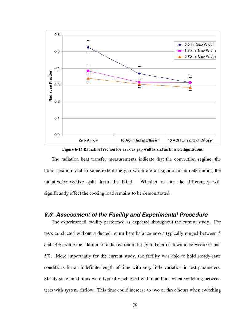
79
0.0
0.1
0.2
0.3
0.4
0.5
0.6
Zero Airflow 10 ACH Radial Diffuser 10 ACH Linear Slot Diffuser
Rad
iati
veF
ract
ion
0.5 in. Gap Width
1.75 in. Gap Width
3.75 in. Gap Width
Figure 6-13 Radiative fraction for various gap widths and airflow configurations
The radiation heat transfer measurements indicate that the convection regime, the
blind position, and to some extent the gap width are all significant in determining the
radiative/convective split from the blind. Whether or not the differences will
significantly effect the cooling load remains to be demonstrated.
6.3 Assessment of the Facility and Experimental ProcedureThe experimental facility performed as expected throughout the current study. For
tests conducted without a ducted return heat balance errors typically ranged between 5
and 14%, while the addition of a ducted return brought the error down to between 0.5 and
5%. More importantly for the current study, the facility was able to hold steady-state
conditions for an indefinite length of time with very little variation in test parameters.
Steady-state conditions were typically achieved within an hour when switching between
tests with system airflow. This time could increase to two or three hours when switching
80
from a zero airflow test to a test with system airflow, due to the thermal capacity of the
room surfaces. Therefore, each test only required roughly four to six hours to capture
three hours of steady-state data and two sets of radiative heat flux measurements. The
efficiency of the facility thus allowed for over 60 tests to be conducted in less than two
months time.
The quickness of each test was also a testament to the experimental procedure and the
Chantrasrisalai thermal model (Chantrasrisalai 2007a). Considering the fenestration
power dissipation was directly measured a heat balance was not required, reducing the
need to completely seal the test room between each test and speeding the entire process.
Also the combining of the innermost glazing and Venetian blind layers in the thermal
model, eliminated the need for timely, expensive and complex instrumentation. Instead a
net radiometer was able to directly measure the radiant heat fluxes, which were used to
back out all other important parameters.
The instrumentation was also very reliable and mostly provided reasonable
uncertainty with few exceptions. The watt-transducer connected to the Venetian blinds
had unacceptably high uncertainty and should be replaced before further studies are
conducted. The watt-transducer was originally selected for its high maximum current
rating, though this capability was never required and a more accurate transducer could
have been utilized. Although this transducer produced very large uncertainties, it did not
have a large effect on the uncertainty associated with the final results. The only other
measurement that produced large uncertainties was the window panel temperature
measurements. This uncertainty was caused by the large temperature gradient found on
the panel and produced large uncertainty in the final results of a limited number of tests.

81
Therefore, it is recommended that steps to reduce this temperature gradient or increase
instrumentation be taken before future work is conducted.
Overall the facility and experimental procedure proved to be very efficient and
reliable. The instrumentation provided very accurate and repeatable measurements,
resulting in very reasonable uncertainties in the final results.
82
7 Conclusions
7.1 Assessment of the ResultsPrevious thermal models in the literature of fenestration systems with shading from a
Venetian blind have either become obsolete with the advancement of glazing technology
or require complicated and expensive experimental procedures, making their validation
impractical and severally detracting from their usefulness. Due to the complexity of
previous thermal models, researchers at Lawrence Berkeley Laboratory developed a
simplified layer model. This model has been hampered by the limited amount of
experimentally determined coefficients. Canadian researchers also performed
experiments to validate a numerical simulation code. Their experimental studies and
numerical model, however, both assumed room airflow would have little effect on the
thermal properties of the fenestration systems. Furthermore, their papers only presented
data for the center-of-glass region of the innermost glazing limiting its usefulness and
making a direct comparison with the current research impossible.
The current research developed the experimental facility required to support the
Chantrasrisalai thermal fenestration model, explored the accuracy of the natural
convection assumption, and examined the significance of several other experimental
parameters. Radiant fractions for the entire complex fenestration system were presented
for 54 tests, including five airflow rates, three gap width and three slat angles. These
tests showed that the radiant fraction had a strong dependency on the system airflow rate,
with one airflow rate providing a greater than 29% reduction in radiant fraction over the
83
natural convection case. Fenestration temperature profiles captured by an infrared
camera showed temperature profiles were also greatly affected by the mechanically
driven flows.
Airspeed tests and preliminary flow visualizations were also conducted to
characterize the pattern for the various flow rates. Results of these tests showed a strong
buoyantly driven plume around the blinds. The strength of this plume was increased with
an increase in system airflow rate during tests with a radial diffuser as the nearby return
grille actually increased the upward air velocity. During tests with the linear slot diffuser,
the buoyant plume caused the wall jet to separate near the top of the fenestration system
resulting in strong mixed and circulating flows.
The effect of the mechanically driven jet on the airflow pattern around the
fenestration unit and thus its effect on the radiative/convective splits, indicates that
natural and mixed convection regimes should be differentiated between in the thermal
fenestration model. Using the natural convection assumption under mixed convection
conditions, could result in errors of up to 40% in the radiative fraction. The
Chantrasrisalai thermal model, which combined the innermost glazing layer and the
Venetian blinds into a single layer, vastly simplified the experimental procedure while
still maintaining the ability to examine the effect of room airflows and configurations.
7.2 Future Work and RecommendationsBefore the Chantrasrisalai model will become truly useful, heat transfer correlations
need to be developed. Although the current study successfully completed a limited
parametric set of experiments, much more experimental work is required before these
correlations could be developed. The correlations will likely require even more
84
parameters than were tested by the current study, including fenestration emissivity,
mounting position of the blinds and more room configurations. Efforts should also focus
on characterizing the flow field around the fenestration system, which will likely require
advanced flow visualization techniques such as particle imaging velocimetry. The
characterization of the flow fluid will allow for a better understanding of the heat transfer
phenomenon acting on the fenestration and could be used to validate computational fluid
dynamics models.
Although the facility and the instrumentation performed very well through the
duration of the current study, improvements could still be made.
7.2.1 Facility• At least one set of new window blinds should be constructed following a modified
version of the procedure given by Wilson et al. (2004). The blinds should be
constructed without the hole in the middle of each slat and stronger and/or more
lattice strings should be used to prevent the loss of tension.
• The blind’s coating should be sprayed on, powder coated or other high quality
method that would provide a uniform, smooth surface.
• A valence should be added to the blind’s header to ensure realistic airflow.
• A heat spreading device should be attached to the window panel. This heating
device would dampen the temperature gradient on the panel and decrease the
uncertainty associated with the spatial averaging of the panel temperature
measurements.
• The top of the partition wall should be attached to the actual structure of the test
room, so that the wall may be leveled correctly.
85
• Web cameras should be installed inside the test room so the location and
operation of the traversing mechanism can be verified without entering the room.
• The preventive maintenance procedure outlined in Appendix B should be
followed to ensure proper operation of the HVAC system.
• Five micron water filters should be added to the heat pump circulation loops so
that the tank water can be continuously filtered and prevent iron buildup.
• All electrical and instrumentation wiring should be labeled to allow quicker
maintenance and modification.
• If tests with lower flow rates or higher heat gains are desired a larger or another
cooling coil should be installed. The current chilled water line already has
sufficient capacity to supply another coil.
7.2.2 Instrumentation• The watt-transducer attached to the Venetian blinds should be replaced before any
future studies begin to reduce the very large uncertainty associated with the blind
power measurement.
• A larger motor or a brake should be installed on the Y-axis on the traversing
mechanism to prevent the instrument attachment from “falling” when the control
program is restarted.
• Before a new study begins the DAC control board should be sent in for servicing
to fix the five burned out channels.
• Directional airspeed probes could be used to gain a better understanding of the
flow field adjacent to the fenestration, while still allowing for a quick and simple
test procedure.

86
References
ASHRAE. 1999. ANSI/ASHRAE Standard 51-1999, Laboratory Methods of Testing Fans
for Aerodynamic Performance Rating. Atlanta, GA: ASHRAE.
ASHRAE. 2005. ASHRAE Handbook - Fundamentals. Atlanta, GA: ASHRAE.
Beckwith, T. G., R. D. Marangoni, and J. H. Lienhard V. 1993. Mechanical
Measurements, Fifth Edition. Reading, MA: Addison-Wesley.
Carroll, C. 2007. Personal Communication. Oklahoma State University, Stillwater, OK.
Chantrasrisalai, C. 2007a. Optical and Thermal Fenestration Models for Building Load
Calculations. Ph.D Thesis, Oklahoma State University, Department of Mechanical
and Aerospace Engineering, Stillwater, OK. Advised by: Dan Fisher.
Chantrasrisalai, C. 2007b. Personal Communication. Oklahoma State University,
Stillwater, OK.
Collins, M. and S. J. Harrison. 1999. Calorimetric measurement of the inward-flowing
fraction of absorbed solar radiation in venetian blinds. ASHRAE Transactions 105:
1022-1030.
Collins, M. and S. J. Harrison. 2004. Calorimetric analysis of the solar and thermal
performance of windows with interior louvered blinds. ASHRAE Transactions
110(1): 474-485.
Collins, M., S. J. Harrison, D. Naylor and P. H. Oosthuizen. 2002. Heat transfer from an
isothermal vertical surface with adjacent heated horizontal louvers: Validation.
Journal of Heat Transfer 124(6): 1078-1087.
87
Collins, M., D. Naylor, S. J. Harrison and P. H. Oosthuizen. 2001. An interferometric
study of convective heat transfer from an irradiated complex window assembly.
American Society of Mechanical Engineers, New York, NY, United States.
DOE. 2007. EnergyPlus Engineering Document: the Reference to EnergyPlus
Calculations, United States Department of Energy.
Duarte, N., D. Naylor, P. H. Oosthuizen and S. J. Harrison. 2001. An interferometric
study of free convection at a window glazing with a heated venetian blind. HVAC
and R Research 7(2): 169-184.
Fisher, D. and C. Chantrasrisalai. 2006. ASHRAE 1282-RP LIGHTING HEAT GAIN
DISTRIBUTION IN BUILDINGS Final Report. RP-1282. Stillwater, OK: ASHRAE.
Fisher, D. E. 1995. An Experimental Investigation of Mixed Convection Heat Transfer in
a Rectangular Enclosure. Ph. D. Thesis, University of Illinois at Urbana-Champaign,
Urbana, Illinois. Advised by: C.O. Pedersen.
Fisher, D. E. and C. O. Pedersen. 1997. Convective heat transfer in building energy and
thermal load calculations. ASHRAE Transactions 103(pt 2): 137-148.
Hern, S. A. 2004. Design of an Experimental Facility for Hybrid Ground Source Heat
Pump Systems. Master's Thesis, Oklahoma State University, Mechanical and
Aerospace Engineering, Stillwater, OK. Advised by: D. Fisher.
Hosni, M. H., B. W. Jones, J. M. Sipes and Y. Xu. 1998. Total heat gain and the split
between radiant and convective heat gain from office and laboratory equipment in
buildings. ASHRAE Transactions 104(1A): 356-365.
Incropera, F. P. and D. P. Dewitt. 2002a. Fundamentals of Heat and Mass Transfer, Fifth
Edition. New York, NY: John Wiley & Sons, inc.
88
Incropera, F. P. and D. P. DeWitt. 2002b. Introduction to Heat Transfer, Fourth Edition.
New York, NY: John-Wiley and Sons.
Jones, B. W., M. H. Hosni and J. M. Sipes. 1998. Measurement of radiant heat gain from
office equipment using a scanning radiometer. ASHRAE Transactions 104(1B):
1775-1782.
Klems, J. H. 1994a. New method for predicting the solar heat gain of complex
fenestration systems - I. Overview and derivation of the matrix layer calculation.
ASHRAE Transactions 100(1): 1065-1072.
Klems, J. H. 1994b. New method for predicting the solar heat gain of complex
fenestration systems - 2. Detailed description of the matrix layer calculation.
ASHRAE Transactions 100(1): 1073-1086.
Klems, J. H. and G. O. Kelley. 1996. Calorimetric measurements of inward-flowing
fraction for complex glazing and shading systems. ASHRAE Transactions 102(1):
947-954.
Klems, J. H. and J. L. Warner. 1995a. Measurement of bidirectional optical properties of
complex shading devices. ASHRAE Transactions 101(1): 791-801.
Klems, J. H. and J. L. Warner. 1997. Solar heat gain coefficient of complex fenestrations
with a venetian blind for differing slat tilt angles. ASHRAE Transactions 103(1):
1026-1034.
Klems, J. H., J. L. Warner and G. O. Kelley. 1995b. A new method for predicting the
solar heat gain of complex fenestration systems. LBL-36995. Berkeley, CA:
Lawrence Berkeley National Laboratory.
89
Kline, S. J. and F. A. McClintock. 1953. Describing Uncertainties in Single-Sample
Experiments. Mechanical Engineering 75: 3-8.
Machin, A. D., D. Naylor, S. J. Harrison and P. H. Oosthuizen. 1998. Experimental study
of free convection at an indoor glazing surface with a Venetian blind. HVAC&R
Research 4(2): 153-166.
MatWeb - Online Material Data Sheet [Tin-Silver Solder (95Sn-5Ag), ASTM B 32
Grade Sn95]. Modified 2006. Retrieved 12/20/2006 from
http://www.matweb.com/search/SpecificMaterial.asp?bassnum=MLSS94
MatWeb - Online Material Data Sheet [AISI Type 304]. Modified 2006. Retrieved
12/20/2006 from
http://www.matweb.com/search/SpecificMaterial.asp?bassnum=MQ304A
Naylor, D., J. Phillips, P. H. Oosthuizen and S. J. Harrison. 2002. Numerical study of
convective and radiative heat transfer from a window glazing with a venetian blind.
Amer. Soc. Heating, Ref. Air-Conditoning Eng. Inc., Atlantic City, NJ.
Naylor, D., H. Shahid, S. J. Harrison and P. H. Oosthuizen. 2006. A simplified method
for modelling the effect of blinds on window thermal performance. International
Journal of Energy Research 30(7): 471-488.
Oh, J. K.-W., J. S. Haberl and L. O. Degelman. 2001. Development of a computer model
for solar simulation and shaded fenestration design. American Society of Mechanical
Engineers, New York, NY 10016-5990, United States, Washington, DC, United
States.
Ohio Semitronics. 2005. AC WATT TRANSDUCER MODEL PC5-. Rev. A. from
https://www.ohiosemitronics.com/pdf/catalog/ac_watt_transducer_modelPC5.pdf.

90
Ohio Semitronics. 2007a. PRECISION AC WATT TRANSDUCER MODEL AGW-.
from
https://www.ohiosemitronics.com/pdf/catalog/precision_ac_watt_transduver_model_
AGW.pdf.
Ohio Semitronics. 2007b. PRECISION AC WATT OR VAR TRANSDUCER MODEL
GW5- & GV5-. from
https://www.ohiosemitronics.com/pdf/catalog/precision_ac_watt_or_var_transducer_
modelsGW5_GV5.pdf.
Ostrach, S. 1953. An Analysis of Laminar Free-Convection Flow and Heat Transfer
about a Flat Plate Parallel to the Direction of the Generating Body Force.: NACA
Technical Report 1111.
Phillips, J., P. H. Oosthuizen, D. Naylor and S. J. Harrison. 2001. Numerical study of
convective and radiative heat transfer from a window glazing with a venetian blind.
HVAC and R Research 7(4): 383-402.
SSHC, Inc. SSHC, Inc. - Enerjoy radiant Heat Panels. Modified 2003. Retrieved from
http://sshcinc.com/BarNone2.htm
Wilson, B., W. Cook and L. Phillippi. 2004. Final Report for Heated Window Blinds
Capstone Design Project: Oklahoma State University. Unpublished Work.
Ye, P., S. J. Harrison, P. H. Oosthuizen and D. Naylor. 1999. Convective heat transfer
from a window with a venetian blind: Detailed modeling. ASHRAE Transactions
105: 1031-1037.

91
Appendix A: Standard Operating Procedures
Procedure for Starting the Control Program
Configure the Fluke Data Acquisition Units
1. Open the program titled “Main Program for Configuring Fluke 2686a Settings”
located in the “stand-alone” sub-folder.
2. Start the program.
3. Hit the browse button next to the “configuration file” textbox and select the
configuration file named “Window Blind Configurations.cgf” located in the
“stand-alone” sub-folder.
4. Click the "read configuration" button.
5. Click the "toolbox initialization" button.
6. Click the "get configurations" button to transfer data from Fluke to PC button.
7. Click the "set configurations" button to transfer data from PC to Fluke button and
wait until the status bar reads “Done.”
8. Press the Stop button, once the program has stopped close it.
Notes:
• This step should be taken before starting or restarting the main program, but does
not have to be completed between each test.
• Ensure any other program that communicated with the Flukes has been stopped or
closed.

92
• If the Fluke DAQ program has been used, the user must select each module from
the instrument list on the left-hand side and uncheck the “Interval Trigger” box.
This set should be performed between steps #4 and #5. If this procedure is not
followed, the main program will crash.
• If instrumentation is added or removed the configuration file can be modified
within this program but the Fluke ports must be turned on within the “Fluke
DAQ” program.
Starting the Main Program
1. Open the program titled “Main Program for WindowBlind Experiments.vi” in the
main folder.
2. Start the program.
3. Click the button that reads “set HVAC Control & Operation” and set the HVAC
control settings as desired.
4. Click the “Start Operation” button.
Notes:
• Starting the main program will cause the Y-axis of the traversing mechanism to
“fall,” therefore the traverse must be repositioned after the main program is
restarted.
• Most HVAC control settings should be left as default, except set points and dead
bands.
• The user should monitor the HVAC system on a require basis to ensure proper
operation.
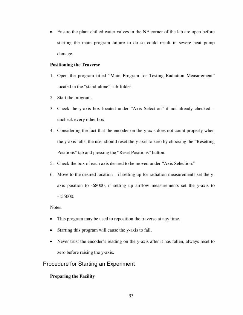
93
• Ensure the plant chilled water valves in the NE corner of the lab are open before
starting the main program failure to do so could result in severe heat pump
damage.
Positioning the Traverse
1. Open the program titled “Main Program for Testing Radiation Measurement”
located in the “stand-alone” sub-folder.
2. Start the program.
3. Check the y-axis box located under “Axis Selection” if not already checked –
uncheck every other box.
4. Considering the fact that the encoder on the y-axis does not count properly when
the y-axis falls, the user should reset the y-axis to zero by choosing the “Resetting
Positions” tab and pressing the “Reset Positions” button.
5. Check the box of each axis desired to be moved under “Axis Selection.”
6. Move to the desired location – if setting up for radiation measurements set the y-
axis position to -68000, if setting up airflow measurements set the y-axis to
-155000.
Notes:
• This program may be used to reposition the traverse at any time.
• Starting this program will cause the y-axis to fall.
• Never trust the encoder’s reading on the y-axis after it has fallen, always reset to
zero before raising the y-axis.
Procedure for Starting an Experiment
Preparing the Facility
94
1. Set window panel system to proper gap width.
2. Completely seal the backside of the window panel using either aluminum foil tape
or black duct tape.
3. Set blinds to proper angle.
4. Check position of the net radiometer to ensure proper location and orientation.
5. Shut and seal the entry door. The door should be sealed with black duct tape;
armiflex should also be placed in large gaps between the blueboard and wall. If a
ducted return is utilized the door does not require sealing.
6. Turn off the lighting.
7. Turn on fans located in the NW and SE corners of the guard space.
8. Plug in fan above the hot water tank.
Setting Test Parameters
1. Make the “Heat Balance Calculation Data” window (HBW) visible on the control
computer. Note: never close this window, if it is closed the main program must
be restarted.
2. Set the supply and return (if required) fans to the desired setting. The system
airflow through the main flow nozzle can be viewed in cubic feet per-minute
under the “Volume Flow Rate / Misc Gains” tap of the HBW.
3. Set the variable transformers for the blinds, window panel and plug load to their
proper settings. The power dissipation of each of these components can be
viewed on under the “Heat Balance” tap of the HBW.
95
4. Set the variable transformer for the guard panel as required for the specific test
conditions. The power dissipated by the guard panel can be reviewed under the
“Volume Flow Rate / Misc Gains” tap of the HBW.
Procedure for Recording Test Data
Heat Balance Data
1. Place a unique name in the “Test Name” text box.
2. Press the “Start Recording HB Data” button.
3. A folder with the test name will be created under the “Measured Data” folder and
two CSV files will appear.
4. The “HB Data.csv” file contains the saved heat balance data. Data from this file
should be moved to the “HB Plot.xls” so heat balance parameters can be plotted.
5. Before ending a test ensure three hours of steady-state data has been collected by
reviewing plots in the “HB Plot.xls” file.
6. To stop recording data press the “Stop Recording HB Data” button.
Notes:
• The main program does not need to be stopped between tests, simply stop
recording data, change the test name, change the test parameters as required and
start recording heat balance data once again.
Radiation Measurements
1. Before starting a radiation measurement, check the “HB Plot.xls” file to ensure
steady-state has been achieved for an adequate period.
2. Open the program titled “Radiation Measurement Loop Main.vi” located in the
“Main SubVIs” sub-folder. Do not start the program.

96
3. Ensure that “Radiation” is selected under the measurement option. This option
can be changed by pressing the ratio button.
4. Ensure that “Operating” is selected under traversing location. This option can be
changed by pressing the ratio button.
5. Click the “Configure Radiation Measurement” button on the main program
window.
6. Browse for the measurement location file desired and selected axis wished to be
moved.
7. Press Done.
8. Press the “Start Radiation Measurement” button.
9. Once the test has been completed rename the “Radiometric Data.csv” if file is not
renamed it will be over-written by the next test.

97
Appendix B: Maintenance Procedures
Preventive Maintenance Schedule
This section of the Appendix was written with the aid of Carroll (2007).
Daily Procedures
1. Check hot and cold water tank level.
2. Drain at least twice as much water as has evaporated to prevent mineral buildup.
3. Refill tank to normal level
Monthly Procedures
1. Check water filters located on the tank fill/drain line, replace with a 5µm if
necessary. Replacement filters can be bought at Lowe’s. The filter housings are
shown in Figure D-1.
2. Check air filters in the fan coil units, replace if necessary. Replacement filters can
be custom ordered from Grainger.
3. Check air filters located in the main system loop, replace with similar filter if
required. One filter is located just upstream of the main cooling coil while the
other is located in the main return header on the third level. Filter housing are
shown in Figure D-3 and Figure D-4.
4. Check the water level in the cooling coil condensate drain and fill if required.
The fill pipe is shown in Figure D-6.

98
5. Ensure proper operation of the safety boards, shown in Figure D-7. This is can
accomplished by disconnecting the timer signal wire or with the program titled
“Main Program for Testing MCC Board IOs.vi” located in the “Stand-Alone VIs”
folder. In the program turn on at least one digital channel then press the Timer
button until it read “Inactive.” The safety board should shut down all equipment
within 60 to 90 seconds.
Quarterly Procedures
1. Shut all isolation valves around each pump. Each pump feeding a coil has three
isolation valves, while the pumps supplying the heat pumps have two isolation
valves. This step will prevent long purge times.
2. Completely drain the hot and cold water tanks.
3. Vacuum up all debris and remaining water from bottom of tank.
4. Clean tank walls. This is best accomplished by spraying water through the high
pressure nozzle onto the walls while scrubbing with a broom.
5. Drain accumulated water.
6. Vacuum up all debris and remaining water from bottom of tank.
7. Clean pump strainers with hydrochloric acid. Replace screen if needed.
8. Completely refill tanks with domestic water.
9. Open all isolation valves around each pump.
10. Open all three-way valves to a setting of 7 with the “Main Program for Testing
MCC Board IOs.vi” located in the “Stand-Alone VIs” folder. Do not turn on the
pumps. Open the two-way valves on the heat pump lines to a setting of 10.

99
11. Purge each line with the outlet of the purge pump flowing to the drain. During
this process more water may need to be added to the tank. This process will
ensure the majority of dirty water is drained.
12. Shut all isolation valves around each pump.
13. Completely drain both tanks.
14. Vacuum up all debris and remaining water from bottom of tank.
15. Completely refill tanks with domestic water.
16. Open all isolation valves around each pump.
17. Open all three-way valves to a setting of 7 with the “Main Program for Testing
MCC Board IOs.vi” located in the “Stand-Alone VIs” folder. Do not turn on the
pumps. Open the two-way valves on the heat pump lines to a setting of 10.
18. Purge each line while its pump is turned on.
Maintenance How-To:
Draining small amounts of water from tanks
1. Open the drain valve shown in Figure D-1.
2. Open the fill/drain valve shown in Figure D-2 for the desired tank.
3. After the desired amount of water has been drained shut both valves.
Draining large amounts of water from tanks
1. Shut all isolation valves around each pump. Each pump feeding a coil has three
isolation valves, while the pumps supplying the heat pumps have two isolation
valves. This step prevents excessive purge times.
2. Connect the suction side of the purge pump to the male hose attachment on the
drain line, shown in Figure D-2.
100
3. Place outlet hose in the drain.
4. Open the fill/drain valve shown in Figure D-2 for the desired tank. Note: Both
tanks can be drained simultaneously; if one tank empties first shut its fill/drain
line.
Filling Tanks
1. Open the domestic water valve shown in Figure D-1. Note: There are two other
valves that may or may not be closed upstream of the valve shown in the figure.
2. Open the fill/drain valve shown in Figure D-2 for the desired tank.
3. After the desired amount of water has been drained shut both valves.
Notes:
• If refilling tanks while the system is on. Add water until the heat pump kicks on.
Once the heat pump starts, wait two minutes before continuing the refilling
process. Failure to do so can cause the control program to ‘safe’ the heat pump,
which requires a program reset.
Purging the Lines
1. Connect the suction side of the purge pump to the male hose connector for the
desired line.
2. If not done during a tank cleaning, place the outlet hose in the tank. If done
during tank cleaning place the outlet hose in the drain.
3. Open valves on the hoses and on the line’s purge connection.
4. If the line is equipped with a three-way valve open it to a setting of 7, if the line
has a two-way valve open to a setting of 10. Only opening the three-way valve
part way ensures that all the air is purged from the system, including bypass pipe.
101
5. Turn on purge pump as well as the line’s pump.
6. After one minute of good water flow out of the discharge hose, shut the isolation
valve on the return pipe (valve on the same pipe as the purge connection).
Closing this valve prevents water from flowing backwards up the return pipe.
Water flow will slow dramatically once this valve has been closed.
7. Once strong water flow has returned for one minute, change the three-way valve
setting to 10. This will keep water from flowing up the bypass line. Water flow
will drop slightly.
8. Continue to purge for at least one more minute of strong water flow.
9. Open the return isolation valve.
10. Turn off purge pump.
11. Shut the valves on the hoses and the line’s purge connection and disconnect
hoses.
Notes:
• Use the program titled “Main Program for Testing MCC Board IOs.vi” located in
the “Stand-Alone VIs” folder to control the valves and pumps during this process.
• Know which line you are working on: The pump order from left to right looking
at the cold water tank is NE fan coil, AHU cooling coil, SW fan coil and chilled
wall. The pump order from left to right looking at the hot water tank is NE fan
coil, AHU cooling coil and SW fan coil. The heat pump supply pumps are
located above the smaller circulating pumps.
• Every line has a purge connection near its return.

102
• If excess air has entered a line some ‘tricks’ may be required to completely purge
a line. These tricks are cover in Appendix C.

103
Appendix C: Troubleshooting
Problem:
Blinds not powering up
• Ensure the GFI has not tripped. The GFI is located above and to the left of the
blind’s variable transformer as shown in Figure D-5. If it has tripped, an amber
light will be illuminated. Reset the GFI by pressing the “reset” button.
• Ensure the variable transformer is turned on. If the variable transformer is on, its
switch should be illuminated red.
• If switch is not illuminated red and the GFI is not tripped, then the problem is on
the source side. Press the “test” button on the GFI.
• If an amber light illuminates the GFI is receiving power. If the GFI is
receiving power, check the internal fuses of the variable transformer. This
requires removing the cover of the transformer’s box. There are two fuses
inside the box; one is on the source side while the other is on the load side.
• If the amber light does not illuminate, ensure the source cord is plugged in (it
is plugged into the South wire mold on the first floor). If cord is plugged in,
check the breaker box and reset any tripped breakers.
• If the switch is illuminated red, the problem is on the load side.

104
• First, ensure the transducer is turned on by turning on the light switch on the
south side of the south entrance door into the test room. This switch powers
all the power transducers as well as the plug load, window panel and guard
panel variable transformers.
• Ensure the blind’s power cord is attached.
• Check the voltage reading at the power transducer. The voltage should be
checked over pins 5 and 6 on the PC5 transducer.
• If there is no voltage across the power transducer, check the internal fuses of
the variable transformer. This requires removing the cover of the
transformer’s box. There are two fuses inside the box; one is on the source
side while the other is on the load side.
• If there is a voltage across the transducer, check the voltage across the blinds.
• If no voltage is present across the blinds but there is across the transducer,
there is a problem in the wiring between the two.
• If there is voltage across the blind but no power, there is a bad connection in
the blind’s wiring. The bad spot in the blind’s wiring can be found by
checking the resistance through a set of slats. If very high resistance is found,
the bad connection is located in that set.
Blind’s GFI continuously trips
• The most likely cause of this is something conductive touching a bare spot on the
blinds. Ensure nothing is touching the blinds.
• If GFI continues to trip, this could be a sign of a loss wire somewhere
downstream of the GFI.

105
Plug load, window panel and/or guard panel not powering up
• Ensure the transducers are turned on by turning on the light switch on the south
side of the south entrance door into the test room. This switch powers all the
power transducers as well as the plug load, window panel and guard panel
variable transformers.
• Check the circuit breaker box on the first floor of the lab. Reset any tripped
circuit breakers.
• Ensure the component is plugged into its source cord coming from the transducer
and transformer.
• Check voltage at the female side of the plug.
• If there is no voltage at the plug, the problem is upstream of the plug. Open
the variable transformers case and check the voltages to further isolate the
problem.
• If there is voltage at the plug, the problem is with the load component or its
wiring.
Heat pumps will not turn on
• Attempt to manually turn on the heat pump in the main program. Click the button
that reads “set HVAC Control & Operation” click the desired heat pump tap,
select manual operation then press the “on/off button” until it becomes light
green. If the heat pump turns on within a minute, everything is working properly.
Switch the operation back to automatic.
• If the heat pump channel does not turn on under manual operation, then the
program must be restarted because the heat pump has been “safed” by the
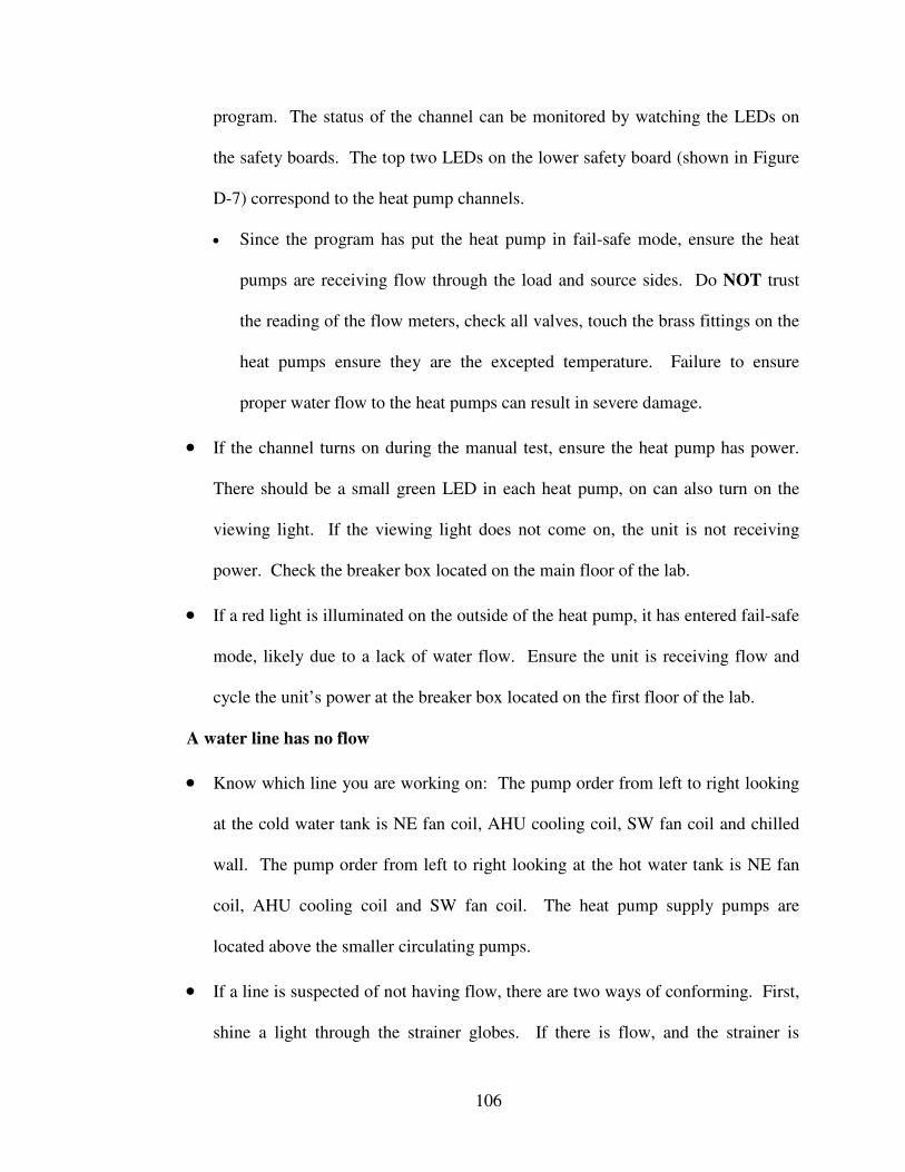
106
program. The status of the channel can be monitored by watching the LEDs on
the safety boards. The top two LEDs on the lower safety board (shown in Figure
D-7) correspond to the heat pump channels.
• Since the program has put the heat pump in fail-safe mode, ensure the heat
pumps are receiving flow through the load and source sides. Do NOT trust
the reading of the flow meters, check all valves, touch the brass fittings on the
heat pumps ensure they are the excepted temperature. Failure to ensure
proper water flow to the heat pumps can result in severe damage.
• If the channel turns on during the manual test, ensure the heat pump has power.
There should be a small green LED in each heat pump, on can also turn on the
viewing light. If the viewing light does not come on, the unit is not receiving
power. Check the breaker box located on the main floor of the lab.
• If a red light is illuminated on the outside of the heat pump, it has entered fail-safe
mode, likely due to a lack of water flow. Ensure the unit is receiving flow and
cycle the unit’s power at the breaker box located on the first floor of the lab.
A water line has no flow
• Know which line you are working on: The pump order from left to right looking
at the cold water tank is NE fan coil, AHU cooling coil, SW fan coil and chilled
wall. The pump order from left to right looking at the hot water tank is NE fan
coil, AHU cooling coil and SW fan coil. The heat pump supply pumps are
located above the smaller circulating pumps.
• If a line is suspected of not having flow, there are two ways of conforming. First,
shine a light through the strainer globes. If there is flow, and the strainer is

107
somewhat dirty, circulating debris should be seen. The cold water return pipes
are also high enough in the tank to check flow rate through by feel. Place you
hand at the end of the return and bypass pipes flow should be felt through at least
one pipe.
• If the strainer and/or hand test reveal there is no flow. Check pump operation. A
slight vibration should be felt; temperature is not an accurate indicator of
operation. If pump is not operating, check to ensure its channel has an
illuminated LED on the safety board.
• If the channel is not on, check the DAS board.
• If the channel is on and the pump is not operating, check to ensure it is
receiving power.
• If the pump is receiving power and the channel is on, the pump has likely
entered fail-safe mode from thermal overload, turn off its channel and allow it
to cool. Purge line before turning channel back on.
• If pump will not operate after being turning off for some time (up to a few
hours), it has likely failed and needs replaced
• If there is no flow and the pump is operating, purge the line following the purge
procedure give in Appendix B.
• If there is flow through the strainer and/or the bypass pipe, check the operation of
the three-way valve with the program titled “Main Program for Testing MCC
Board IOs.vi” located in the “Stand-Alone VIs” folder.

108
• If the valve does not respond to inputs, check the power supply located in the
rack-mount, labeled in Figure D-9. The voltage should be set to 24Vac and
the lower green light next to the plug should be illuminated.
• If the power supply is functioning properly, check the output from the DAC
board. The DAC board has a tendency to loss channels.
• If the DAC channel is functioning, check the power and signal at the valve.
Drain line is not draining
• The drain line works with a siphon, therefore if a large amount of air is in the line
it will not have proper suction.
• Run domestic water through line to push out the air.
Standard purge procedure does not work
• There are several methods to aid the purging process.
• Fill the purge hoses with water, by sucking water though the pump from the tank.
Once hoses are full of water, connect the suction hose back to the purge connector
on the pipe. The water in the line will provide extra suction power, to help prime
the line. This process may need to be repeated several times.
• The lines can also be purged backwards.
• If the line is supplying a coil. First, turn off the line pump and open the three-
way valves to a setting of 7. Remove the strainer globe so that water can exit
the line at the strainer connector. Place the suction hose in the tank and
connect the discharge hose of the purge pump to the purge connector on the
line. Purge until strong water flow is coming out of strainer hosing. Turn off

109
purge pump and replace the strainer globe. Turn on the line pump and follow
the standard purge procedure.
• If the line is supplying a heat pump. The heat pumps have an internal check
valve; therefore the heat pump must be bypassed. First, turn off the line pump
and open the two-way valves to a setting of 10. From this point on follow the
procedure for the coil lines.
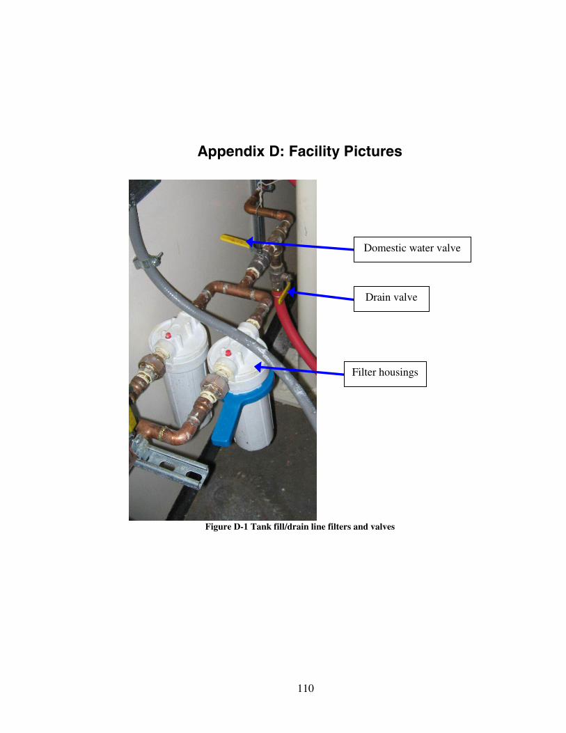
110
Appendix D: Facility Pictures
Figure D-1 Tank fill/drain line filters and valves
Domestic water valve
Drain valve
Filter housings
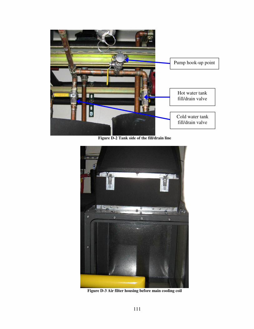
111
Figure D-2 Tank side of the fill/drain line
Figure D-3 Air filter housing before main cooling coil
Pump hook-up point
Cold water tankfill/drain valve
Hot water tankfill/drain valve
112
Figure D-4 Air filter housing on third level
Figure D-5 Variable transformer bank
Blinds’ GFI
Plug load variac
Window panelvariac
Guard panelvariac
Blinds’ variac
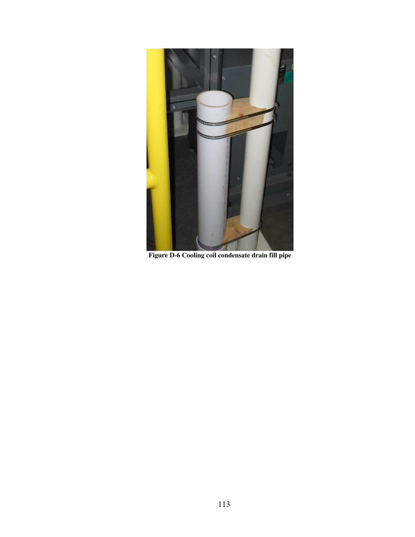
113
Figure D-6 Cooling coil condensate drain fill pipe
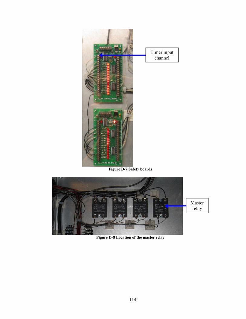
114
Figure D-7 Safety boards
Figure D-8 Location of the master relay
Masterrelay
Timer inputchannel
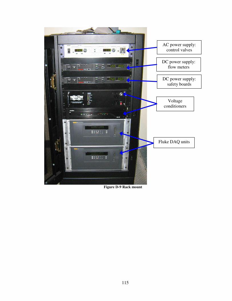
115
Figure D-9 Rack mount
Fluke DAQ units
Voltageconditioners
DC power supply:safety boards
DC power supply:flow meters
AC power supply:control valves
116
Appendix E: Thermocouple Calibration Summary
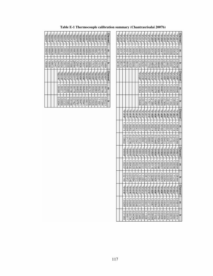
117
Table E-1 Thermocouple calibration summary (Chantrasrisalai 2007b)
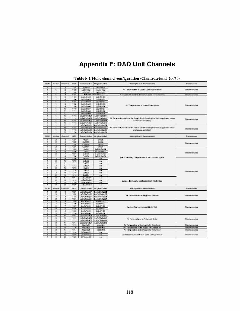
118
Appendix F: DAQ Unit Channels
Table F-1 Fluke channel configuration (Chantrasrisalai 2007b)
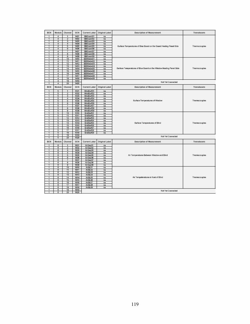
119
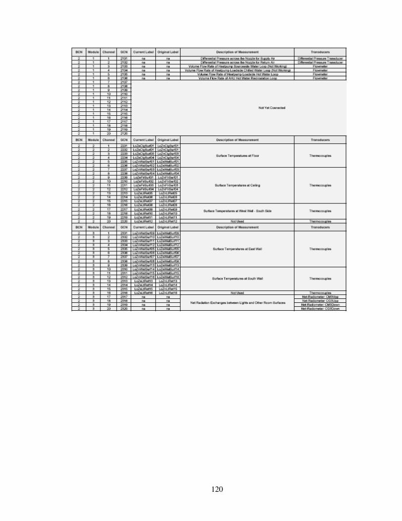
120
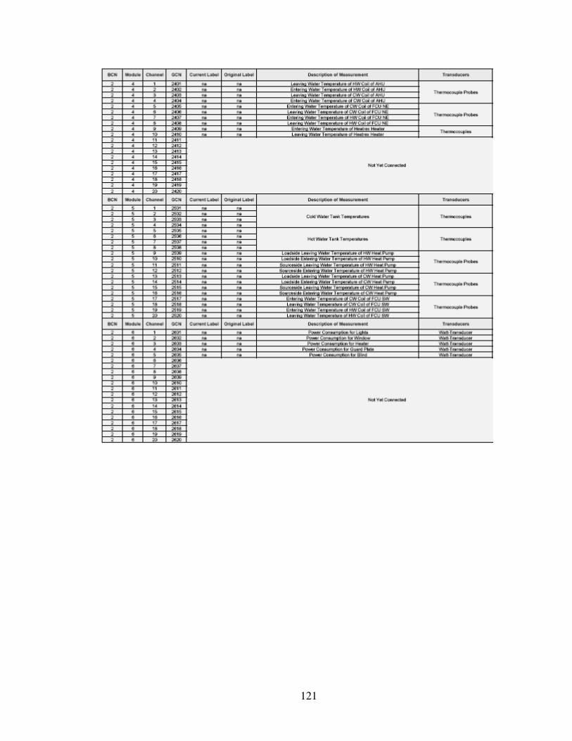
121
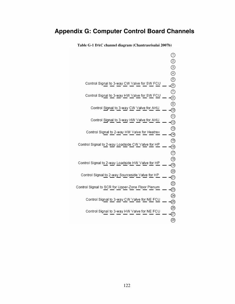
122
Appendix G: Computer Control Board Channels
Table G-1 DAC channel diagram (Chantrasrisalai 2007b)
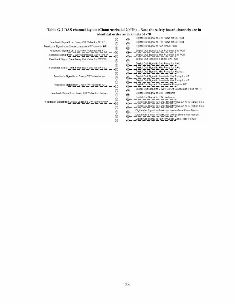
123
Table G-2 DAS channel layout (Chantrasrisalai 2007b) – Note the safety board channels are inidentical order as channels 51-70
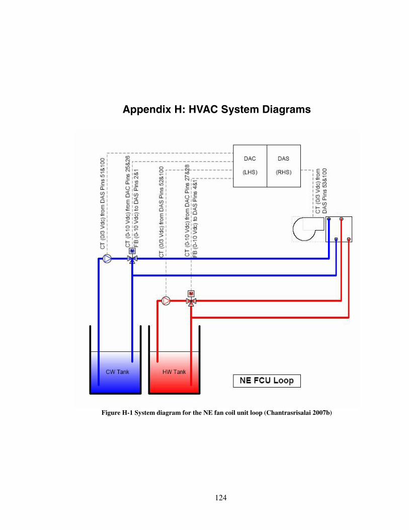
124
Appendix H: HVAC System Diagrams
Figure H-1 System diagram for the NE fan coil unit loop (Chantrasrisalai 2007b)
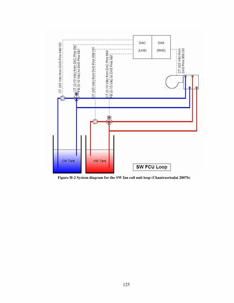
125
Figure H-2 System diagram for the SW fan coil unit loop (Chantrasrisalai 2007b)
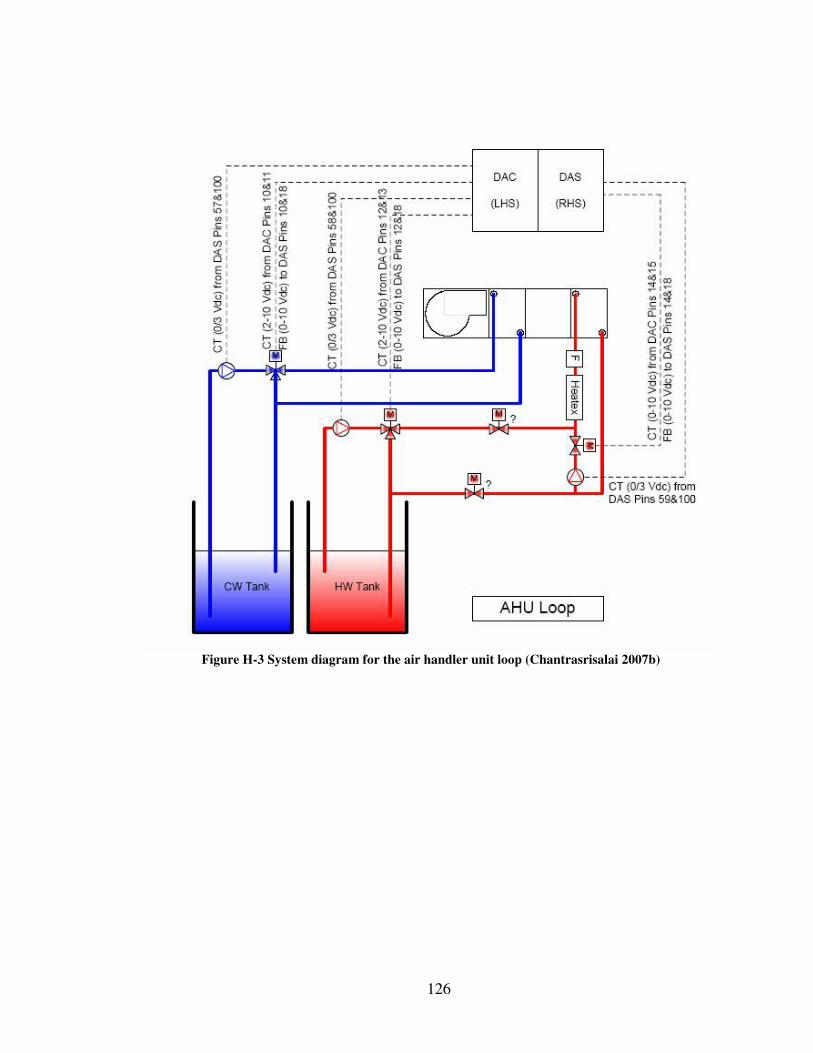
126
Figure H-3 System diagram for the air handler unit loop (Chantrasrisalai 2007b)
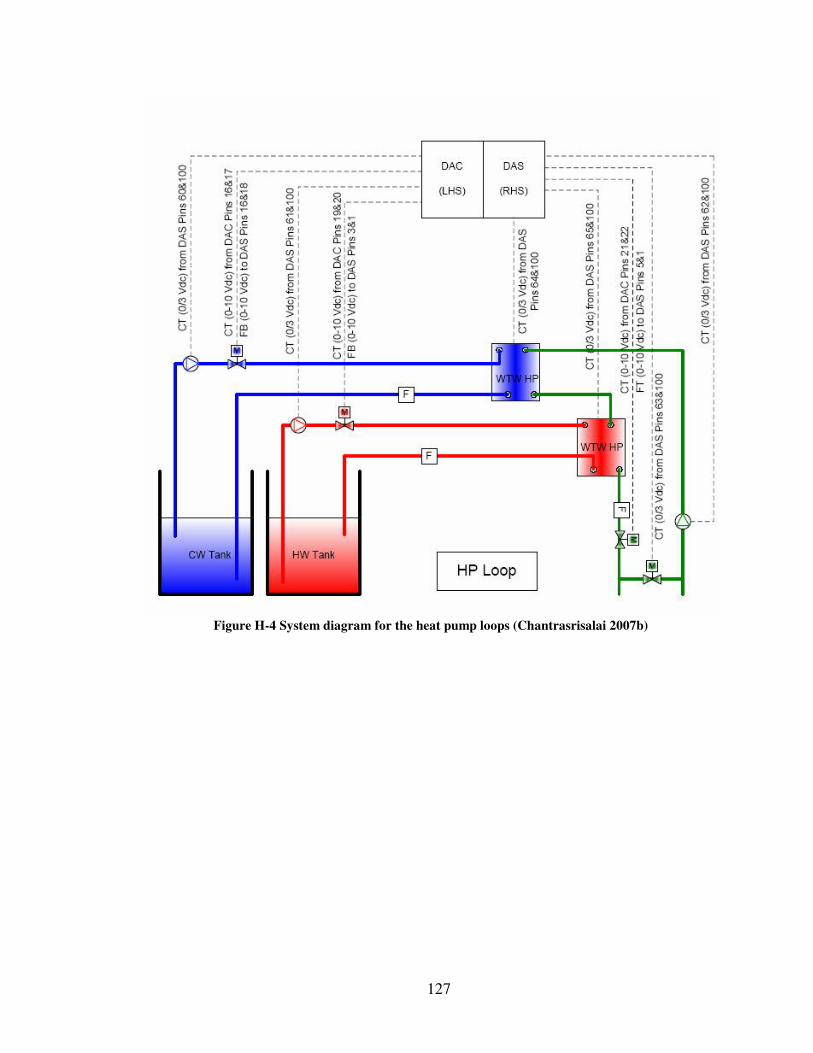
127
Figure H-4 System diagram for the heat pump loops (Chantrasrisalai 2007b)
VITA
Barry Allan Wilson
Candidate for the Degree of
Master of Science
Thesis: EXPERIMENTAL MEASUREMENT OF RADIATION HEAT TRANSFERFROM COMPLEX FENESTRATION SYSTEMS
Major Field: Mechanical Engineering
Biographical:
Personal Data: Born in Broken Arrow, Oklahoma on May 1, 1984, the son ofTed and Susan Wilson.
Education: Graduated from American School of Correspondence High School,Lansing, Illinois in August 2001. Received a Bachelor of Sciencedegree in Mechanical Engineering from Oklahoma State University,Stillwater, Oklahoma in May 2005. Completed the requirements for theMaster of Science degree with a major in Mechanical Engineering atOklahoma State University in May 2007.
Experience: Employed as an amusement manager with Superplay, Inc. fromMay 2002 to May 2007. Interned at Boeing/Spirit Aerosystems fromMay 2005 to August 2005. Employed by Oklahoma State University,Department of Mechanical and Aerospace Engineering, as a graduateresearch assistant from August 2005 to present.
Professional Memberships: Pi Tau Sigma
Name: Barry Allan Wilson Date of Degree: May, 2007
Institution: Oklahoma State University Location: Stillwater, Oklahoma
Title of Study: EXPERIMENTAL MEASUREMENT OF RADIATION HEATTRANSFER FROM COMPLEX FENESTRATION SYSTEMS
Pages in Study: 125 Candidate for the Degree of Master of Science
Major Field: Mechanical Engineering
Scope and Method of Study: The scope of this study was the design and validation of afacility for the measurement of heat transfer from complex fenestration systems.This facility will allow future work to develop heat transfer correlations and toperform complex flow visualization in order to characterize the adjacent airflow.In addition to the facility design and validation, a limited parametric set of over60 tests was performed to provide preliminary results and to validate theexperimental procedure. The acceptability of the literature’s assumption ofnatural convection was also tested, with radiation measurements and preliminaryairflow analysis.
Findings and Conclusions: A well instrumented facility for the measurement of heattransfer from complex fenestration systems was built and validated. The facilityprovided very accurate measurements based on the uncertainty analysis. Resultsare also highly repeatable. Results of the airflow analysis showed a strongbuoyant plume was always present on the fenestration, even at high flow ratesfrom an overhead linear slot diffuser. Although the buoyant plume was alwayspresent, system airflow still had an affect on temperature profiles and createdareas of mixed convection. Radiation data showed system airflow did have asignificant affect on the heat transfer with some airflow rates showing a 40%reduction in radiant fraction over the zero-airflow case. Future work will be tofull characterize the airflow adjacent to the fenestration and to develop heattransfer correlations.
ADVISER’S APPROVAL: Dr. Dan Fisher g