Experimental measurements of break-up

reactions to study alpha clustering in

carbon-12 and beryllium-9

by

Robin Smith

A thesis submitted toThe University of Birmingham

for the degree ofDoctor of Philosophy

School of Physics and AstronomyCollege of Engineering and Physical Sciences

University of BirminghamJuly 2017

University of Birmingham Research Archive

e-theses repository This unpublished thesis/dissertation is copyright of the author and/or third parties. The intellectual property rights of the author or third parties in respect of this work are as defined by The Copyright Designs and Patents Act 1988 or as modified by any successor legislation. Any use made of information contained in this thesis/dissertation must be in accordance with that legislation and must be properly acknowledged. Further distribution or reproduction in any format is prohibited without the permission of the copyright holder.

Abstract

Due to the high binding energy of the ↵-particle, this object can preform in heavier atomic

nuclei. This work explores ↵-clustering in 9Be and 12C by measuring their nuclear break-up.

For 9Be, it has been proposed that the two ↵-particles of the unstable 8Be nucleus are bound

together by a covalently shared neutron. This thesis reports the observation of a state in 9Be

at 3.8 MeV through the 9Be(4He,↵)↵↵n reaction. By comparing its reduced width with that

of a potential mirror analogue in 9B, its angular momentum was shown to be J < 7/2. This

is consistent with a hitherto unmeasured 3/2+ molecular binding configuration state. The 12C

nucleus is thought to consist of three ↵-clusters and its famous Hoyle state has been shown

to possess an unusually large volume. Due to its low density, this state may behave like a

Bose-Einstein condensate, where the fermonic structures of the constituent ↵-particles are no

longer important. By precisely measuring the decay of the Hoyle state into three ↵-particles,

through the 12C(4He,↵)3↵ reaction, an upper limit for the direct 3↵ decay branch of 0.047%

was obtained. This lies below predictions for the decay of a condensate state, casting doubt on

this interpretation.

To my Mom and Dad, Jane and Ray Smith,

for your support, encouragement

and belief in me.

Acknowledgements

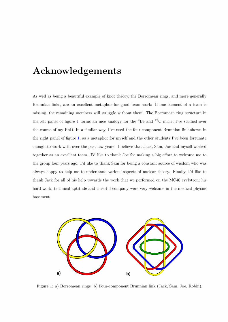
As well as being a beautiful example of knot theory, the Borromean rings, and more generally

Brunnian links, are an excellent metaphor for good team work: If one element of a team is

missing, the remaining members will struggle without them. The Borromean ring structure in

the left panel of figure 1 forms an nice analogy for the 9Be and 12C nuclei I’ve studied over

the course of my PhD. In a similar way, I’ve used the four-component Brunnian link shown in

the right panel of figure 1, as a metaphor for myself and the other students I’ve been fortunate

enough to work with over the past few years. I believe that Jack, Sam, Joe and myself worked

together as an excellent team. I’d like to thank Joe for making a big e↵ort to welcome me to

the group four years ago. I’d like to thank Sam for being a constant source of wisdom who was

always happy to help me to understand various aspects of nuclear theory. Finally, I’d like to

thank Jack for all of his help towards the work that we performed on the MC40 cyclotron; his

hard work, technical aptitude and cheerful company were very welcome in the medical physics

basement.

a) b)

Figure 1: a) Borromean rings. b) Four-component Brunnian link (Jack, Sam, Joe, Robin).

Of course, there are so many more people who have made my experience as a PhD student

at Birmingham so memorable. Many thanks to Carl and Martin for being excellent supervisors,

providing me with the space to exercise my own creativity but always making time to help me

out and proof-read work. To Tzany for her nuclear physics help, general support and continual

supply of vegan sweets. To Neil for his climbing help and for all of his assistance with RES8 and

other aspects of my analysis. Thank you to Peter Jones, Garry Tungate, Dave Forest, Gordon

Squier and various other group members for their useful feedback to practice talks and excellent

support and guidance as teaching colleagues. Thank you to David Parker and other members

of the Birmingham cyclotron sta↵ for their hard work and patience during the experiments.

Thank you to Paul Jagpal for his expertise in nuclear electronics and advice. Thank you to

Mark Caprio, Pieter Maris and James Vary for a number of illuminating discussions about ab

initio nuclear theory, which taught me a lot. Finally, thank you to the sta↵ in the physics

workshop and stores, who have been very helpful in sourcing materials and building equipment

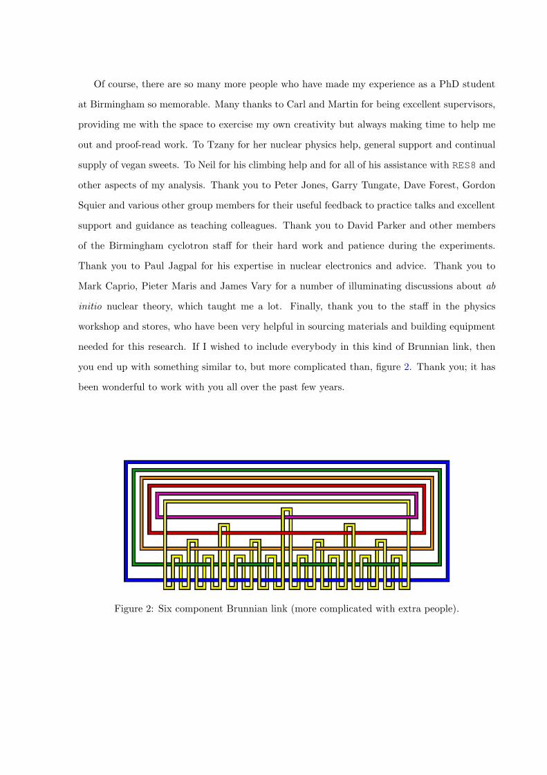
needed for this research. If I wished to include everybody in this kind of Brunnian link, then

you end up with something similar to, but more complicated than, figure 2. Thank you; it has

been wonderful to work with you all over the past few years.

Figure 2: Six component Brunnian link (more complicated with extra people).

Author contribution

The skills and e↵orts of many people have come together to lead to the research outcomes

detailed in this thesis. This is particularly pertinent when considering the set-up of the experi-

ments and the acquisition of data. My own role in this research is detailed below.

Regarding the structure of 9Be, which is detailed in chapter 4, I did not attend the experiment

used to obtain this data set. I retrieved the calibrated data upon starting my PhD. However,

the data analysis is my own. This involved writing sort codes to perform the primary data

analysis, in order to generate clean excitation spectra for 9Be. I performed Monte-Carlo simu-

lations and wrote a Voigt curve fitting code in order to extract information from these spectra.

The calculation of reduced widths, the comparison with the 9B mirror nucleus and theoretical

interpretation were performed by me. I wrote the papers that were published on this research.

I was the lead investigator into the structure of the 12C Hoyle state detailed in chapter 5.

I performed Monte-Carlo simulations in order to optimise the experimental set-up, lead the

physical construction of the apparatus, calibrated the data and was in attendance as the data

were being acquired during a long experimental campaign. In addition to this, I performed

the entirety of the data analysis. This included writing the main primary analysis sort code

to generate the Dalitz plots. The Monte-Carlo simulations of the sequential and direct decay

processes were also performed by me, along with the statistical analysis used to determine upper

limits for the direct decay contributions. Calculations of the expected direct decay branching

ratio, based on phase space and Coulomb barrier penetrabilities, were also my work. I wrote

the paper that was published on this research.

List of publications

Experimental

R. Smith, Tz. Kokalova, et al. New Measurement of the Direct 3↵ Decay from the 12C Hoyle

State, Phys. Rev. Lett. 119 (2017).

R. Smith, M. Freer, C. Wheldon, N. Curtis, Tz. Kokalova, et al. Disentangling unclear nuclear

breakup channels of beryllium-9 using the three-axis Dalitz plot. Journal of Physics: Conf. Series

863 (2017).

R. Smith, C. Wheldon, M. Freer, N. Curtis, Tz. Kokalova, et al. Evidence for a 3.8 MeV state

in 9Be. Physical Review C 94 (2016).

S. Bailey, M. Freer, Tz. Kokalova, C. Wheldon, R. Smith, J. Walshe, et. al. Alpha clustering

in Ti isotopes: 40,44,48Ca + ↵ resonant scattering. In EPJ Web of Conferences 113 08002 (2016).

R. Smith, C. Wheldon, M. Freer, N. Curtis, Tz. Kokalova, et al. Breakup branches of Borromean

beryllium-9. Proceedings of Nuclear Structure and Dynamics 15. Vol. 1681. AIP Publishing,

(2015).

Theoretical

M. A. Caprio, P. Maris, J. P. Vary, and R. Smith, Collective rotation from ab initio theory, Int.

J. Mod. Phys. E 24, 1541002 (2015).

M. A. Caprio, P. Maris, J. Vary, and R. Smith, Emergence of rotational bands in ab initio no-

core configuration interaction calculations, Rom. J. Phys. 60, 5-6 (2015).

J. P. Vary, P. Maris, H. Potter, M. A. Caprio, R. Smith, S. Binder, A. Calci, J. Langhammer,

R. Roth, H. M. Aktulga et. al. Ab Initio No Core Shell Model - Recent Results and Further

Prospects, Proceedings of International Conference “Nuclear Theory in the Supercomputing Era

2014” (NTSE-2014), Pacific National University, Khabarovsk, Russia, June 23-27, 2014 (2015).

Have you ever noticed that the words

“nuclear” and “unclear” are so similar?

– trad.

Contents

Contents

List of figures

List of tables

1 Introduction 1

2 Nuclear structure 5

2.1 The liquid drop model . . . . . . . . . . . . . . . . . . . . . . . . . . . . . . . . . 5

2.2 The spherical shell model . . . . . . . . . . . . . . . . . . . . . . . . . . . . . . . 8

2.3 Nuclear deformation . . . . . . . . . . . . . . . . . . . . . . . . . . . . . . . . . . 11

2.4 Collective rotation . . . . . . . . . . . . . . . . . . . . . . . . . . . . . . . . . . . 15

2.5 ↵-clustering . . . . . . . . . . . . . . . . . . . . . . . . . . . . . . . . . . . . . . . 19

3 Nuclear reactions 25

3.1 Nuclear resonances . . . . . . . . . . . . . . . . . . . . . . . . . . . . . . . . . . . 25

3.2 Introduction to R-Matrix theory . . . . . . . . . . . . . . . . . . . . . . . . . . . 28

4 Molecular structures in the mirror nuclei, beryllium-9 and boron-9 34

4.1 Review of the beryllium-9 nucleus . . . . . . . . . . . . . . . . . . . . . . . . . . 36

4.1.1 Two-centre shell model . . . . . . . . . . . . . . . . . . . . . . . . . . . . 36

4.1.2 Molecular model . . . . . . . . . . . . . . . . . . . . . . . . . . . . . . . . 38

4.1.3 Shell model and no-core shell model calculations . . . . . . . . . . . . . . 41

4.1.4 Experimental review of 9Be . . . . . . . . . . . . . . . . . . . . . . . . . . 42

4.1.5 Mirror nuclei . . . . . . . . . . . . . . . . . . . . . . . . . . . . . . . . . . 44

4.2 Experimental details and apparatus . . . . . . . . . . . . . . . . . . . . . . . . . 47

4.2.1 Notre Dame tandem Van De Graa↵ accelerator . . . . . . . . . . . . . . . 47

4.2.2 Basic reaction dynamics . . . . . . . . . . . . . . . . . . . . . . . . . . . . 51

4.2.3 Detector set-up . . . . . . . . . . . . . . . . . . . . . . . . . . . . . . . . . 52

4.2.4 Electronics and data acquisition . . . . . . . . . . . . . . . . . . . . . . . 57

4.3 Primary analysis . . . . . . . . . . . . . . . . . . . . . . . . . . . . . . . . . . . . 62

4.3.1 Determining the direction and momenta of the detected particles . . . . . 62

4.3.2 Detector front and rear face energy matching . . . . . . . . . . . . . . . . 63

4.3.3 Kinematic lines . . . . . . . . . . . . . . . . . . . . . . . . . . . . . . . . . 64

4.3.4 Q-value spectra . . . . . . . . . . . . . . . . . . . . . . . . . . . . . . . . . 65

4.3.5 Target energy losses correction . . . . . . . . . . . . . . . . . . . . . . . . 67

4.3.6 Decay channel selection . . . . . . . . . . . . . . . . . . . . . . . . . . . . 71

4.3.7 Excitation energy calculation . . . . . . . . . . . . . . . . . . . . . . . . . 74

4.3.8 Further contaminant reaction channels . . . . . . . . . . . . . . . . . . . . 76

4.4 Secondary analysis . . . . . . . . . . . . . . . . . . . . . . . . . . . . . . . . . . . 79

4.4.1 Monte-Carlo simulations . . . . . . . . . . . . . . . . . . . . . . . . . . . . 79

4.4.2 Peak fitting . . . . . . . . . . . . . . . . . . . . . . . . . . . . . . . . . . . 90

4.4.3 Reduced width calculations . . . . . . . . . . . . . . . . . . . . . . . . . . 100

4.5 Interpretation of results . . . . . . . . . . . . . . . . . . . . . . . . . . . . . . . . 104

4.6 Outlook . . . . . . . . . . . . . . . . . . . . . . . . . . . . . . . . . . . . . . . . . 106

5 Investigating the 3↵ break-up modes of the 12C Hoyle state 109

5.1 Introduction . . . . . . . . . . . . . . . . . . . . . . . . . . . . . . . . . . . . . . . 111

5.2 The Hoyle state in stellar nucleosynthesis . . . . . . . . . . . . . . . . . . . . . . 115

5.3 Theoretical models of 12C and the Hoyle state . . . . . . . . . . . . . . . . . . . . 117

5.3.1 Mean field models of 12C . . . . . . . . . . . . . . . . . . . . . . . . . . . 117

5.3.2 Ab initio approaches to 12C . . . . . . . . . . . . . . . . . . . . . . . . . . 118

5.3.3 Antisymmetrised molecular dynamics (AMD) and fermionic molecular dy-

namics (FMD) . . . . . . . . . . . . . . . . . . . . . . . . . . . . . . . . . 120

5.3.4 Cluster models and dynamical symmetries . . . . . . . . . . . . . . . . . . 122

5.3.5 Bose-Einstein Condensates . . . . . . . . . . . . . . . . . . . . . . . . . . 125

5.4 The 3↵ decay of the Hoyle state . . . . . . . . . . . . . . . . . . . . . . . . . . . 129

5.4.1 Structures and 3↵ decay signatures . . . . . . . . . . . . . . . . . . . . . 130

5.4.2 Full three-body calculations . . . . . . . . . . . . . . . . . . . . . . . . . . 132

5.4.3 Decay signatures of an ↵-condensed state . . . . . . . . . . . . . . . . . . 134

5.5 Sequential and direct decay calculations . . . . . . . . . . . . . . . . . . . . . . . 135

5.5.1 Semi-classical approach to barrier transmission . . . . . . . . . . . . . . . 136

5.5.2 Phase space calculations . . . . . . . . . . . . . . . . . . . . . . . . . . . . 142

5.6 Experimental details and apparatus . . . . . . . . . . . . . . . . . . . . . . . . . 146

5.6.1 Birmingham MC40 cyclotron accelerator . . . . . . . . . . . . . . . . . . . 146

5.6.2 Detector set-up . . . . . . . . . . . . . . . . . . . . . . . . . . . . . . . . . 149

5.6.3 Electronics and data acquisition . . . . . . . . . . . . . . . . . . . . . . . 151

5.7 Monte-Carlo simulations . . . . . . . . . . . . . . . . . . . . . . . . . . . . . . . . 153

5.8 Primary analysis and data reduction . . . . . . . . . . . . . . . . . . . . . . . . . 158

5.8.1 Detector energy and position calibration . . . . . . . . . . . . . . . . . . . 159

5.8.2 Detector energy resolution . . . . . . . . . . . . . . . . . . . . . . . . . . . 163

5.8.3 Particle identification telescope, hit multiplicities and hit patterns . . . . 167

5.8.4 Excitation, total energy, and total momentum spectra . . . . . . . . . . . 172

5.8.5 Break-up channel visualisation . . . . . . . . . . . . . . . . . . . . . . . . 181

5.8.6 Dalitz Plots . . . . . . . . . . . . . . . . . . . . . . . . . . . . . . . . . . . 183

5.8.7 Simulated Dalitz plots . . . . . . . . . . . . . . . . . . . . . . . . . . . . . 191

5.8.8 Kinematic fitting . . . . . . . . . . . . . . . . . . . . . . . . . . . . . . . . 197

5.9 Secondary analysis . . . . . . . . . . . . . . . . . . . . . . . . . . . . . . . . . . . 202

5.9.1 Dalitz plot projections . . . . . . . . . . . . . . . . . . . . . . . . . . . . . 202

5.9.2 Frequentist statistical analysis . . . . . . . . . . . . . . . . . . . . . . . . 205

5.9.3 Bayesian statistical analysis . . . . . . . . . . . . . . . . . . . . . . . . . . 210

5.9.4 Summary of results . . . . . . . . . . . . . . . . . . . . . . . . . . . . . . . 215

5.10 Interpretation of Results . . . . . . . . . . . . . . . . . . . . . . . . . . . . . . . . 216

5.11 Outlook . . . . . . . . . . . . . . . . . . . . . . . . . . . . . . . . . . . . . . . . . 218

6 Resistive strip detector improvements 221

7 Summary 236

Appendices 242

A Rotational wave functions 243

B Calculation of the angle of each detected particle 246

C Two-body kinematics 248

D Dalitz plots 251

D.1 Deriving the Dalitz plot coordinates . . . . . . . . . . . . . . . . . . . . . . . . . 251

D.2 Deriving the bounded area of the Dalitz plot . . . . . . . . . . . . . . . . . . . . 253

E Kinematic fitting 256

E.1 Kinematic fitting example . . . . . . . . . . . . . . . . . . . . . . . . . . . . . . . 256

E.2 Kinematic fitting theory . . . . . . . . . . . . . . . . . . . . . . . . . . . . . . . . 261

F Lead author publications 264

References 287

List of Figures

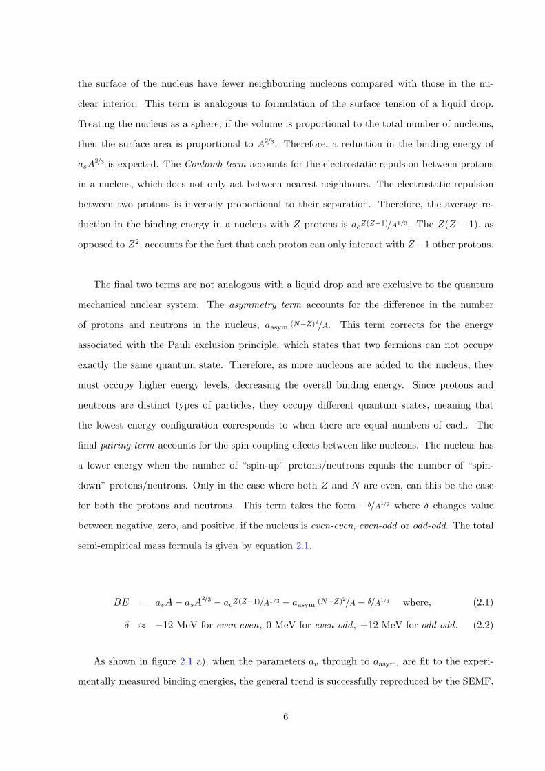
2.1 a) The binding energy per nucleon, BE/A, as a function of mass number, A (for

odd-A isotopes only). The points show experimental data and the red line gives

the prediction of the SEMF. The inset shows the fit residuals. b) The process of

fission through a liquid-drop picture. 1. The configuration with the least surface

energy and the greatest Coulomb energy, 2. & 3. More surface energy and less

Coulomb energy. 4. If the surface + Coulomb energy is greater for the deformed

system, the nucleus will split/fission. Image in b) is modified from reference [12]. 7

2.2 The single-particle energy levels of a Woods-Saxon potential, with (right) and

without (left) the inclusion of spin-orbit splitting. The levels are labelled N`j ,

withN as the principal quantum number, ` as the orbital angular momentum, and

j as the total angular momentum. The numbers to the right of the levels show

the proton/neutron degeneracies. The levels are shown within a Woods-Saxon

potential with the form of equation 2.3. . . . . . . . . . . . . . . . . . . . . . . . 9

2.3 The intrinsic shape of an axially-symmetric deformed nucleus as a function of the

deformation parameter, �2. Image modified from reference [20]. . . . . . . . . . . 11

2.4 The Nilsson single-particle levels as a function of the deformation parameter, ✏2 [6] 13

2.5 a) Definition of the coordinate system and ⌦ quantum number used in the Nilsson

model (adapted from [22]). b) Schematic level splitting as a function of the

deformation parameter, ✏. . . . . . . . . . . . . . . . . . . . . . . . . . . . . . . . 14

2.6 The coupling of intrinsic and collective angular momenta and their projections

onto the deformation (symmetry) axis. . . . . . . . . . . . . . . . . . . . . . . . . 17

2.7 a) The Coriolis force as an artefact of the Earth’s rotation, deflects an object

either in the direction of, or against the direction of, the Earth’s rotational angular

momentum. Image adapted from reference [27]. b) A classical picture of a nucleon

with intrinsic angular momentum, j , coupling to a total angular momentum J ,

with a strength (J · j ). . . . . . . . . . . . . . . . . . . . . . . . . . . . . . . . . . 18

2.8 The excitation of a spherical shoal of mackerel into a two ‘cluster’ structure.

Images from reference [30]. . . . . . . . . . . . . . . . . . . . . . . . . . . . . . . 19

2.9 The Ikeda diagram, which links accessible cluster structures with excitation en-

ergy. Clusters are labelled except for ↵-particles, which are denoted by the green

circles. Image created by Tz. Kokalova and taken from reference [28]. . . . . . . 20

2.10 The binding energy per nucleon (BEPN) as a function of the nucleon number, A,

for a selection of even-A naturally occurring isotopes. Images from reference [32]. 21

2.11 Left: The energy levels of the SHO as a function of the deformation parameter ✏2.

Right: Approximate 8Be nuclear density projections calculated in the HO basis.

Image from reference [6]. . . . . . . . . . . . . . . . . . . . . . . . . . . . . . . . . 22

3.1 The production of unbound resonances in the n +AZ X system. Image modified

from reference [38]. . . . . . . . . . . . . . . . . . . . . . . . . . . . . . . . . . . . 26

3.2 Penetration into the internal nuclear region for di↵erent values of the phase shift,

⇣. The top panel shows the system far away from resonance, and the bottom

panel shows the system on resonance (wave function derivative is zero at the

boundary). The centre panel shows the system for an intermediate value of ⇣.

Image from reference [39]. . . . . . . . . . . . . . . . . . . . . . . . . . . . . . . . 27

3.3 The functional form of the potential for varying centrifugal barriers in the 16O +

208Pb system. Image from reference [43]. . . . . . . . . . . . . . . . . . . . . . . . 29

4.1 The energy levels of the two-centre shell model as a function of the ↵-cluster

separation distance r. Figure from references [54] and [55]. . . . . . . . . . . . . . 37

4.2 The relative alignments of the two p3/2 orbitals with respect to the 9Be deforma-

tion axis for the �- and ⇡-type bonding. Images from reference [6]. . . . . . . . . 38

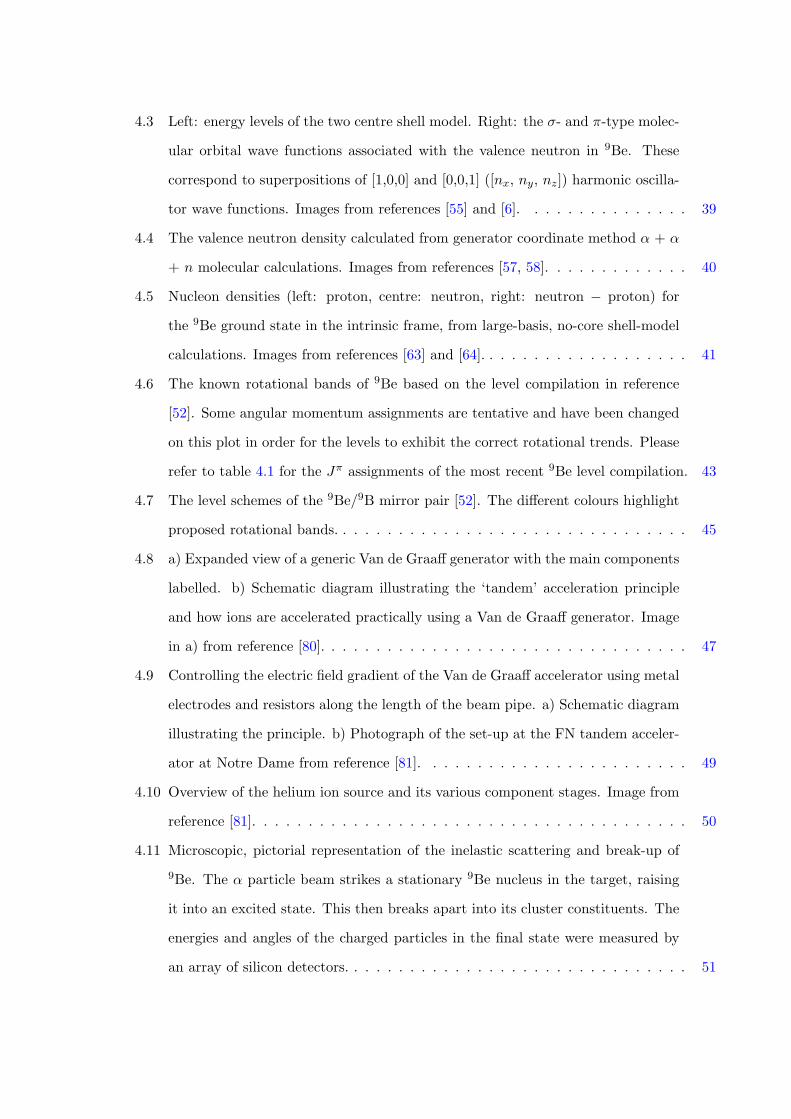
4.3 Left: energy levels of the two centre shell model. Right: the �- and ⇡-type molec-

ular orbital wave functions associated with the valence neutron in 9Be. These

correspond to superpositions of [1,0,0] and [0,0,1] ([nx, ny, nz]) harmonic oscilla-

tor wave functions. Images from references [55] and [6]. . . . . . . . . . . . . . . 39

4.4 The valence neutron density calculated from generator coordinate method ↵ + ↵

+ n molecular calculations. Images from references [57, 58]. . . . . . . . . . . . . 40

4.5 Nucleon densities (left: proton, centre: neutron, right: neutron � proton) for

the 9Be ground state in the intrinsic frame, from large-basis, no-core shell-model

calculations. Images from references [63] and [64]. . . . . . . . . . . . . . . . . . . 41

4.6 The known rotational bands of 9Be based on the level compilation in reference

[52]. Some angular momentum assignments are tentative and have been changed

on this plot in order for the levels to exhibit the correct rotational trends. Please

refer to table 4.1 for the J⇡ assignments of the most recent 9Be level compilation. 43

4.7 The level schemes of the 9Be/9B mirror pair [52]. The di↵erent colours highlight

proposed rotational bands. . . . . . . . . . . . . . . . . . . . . . . . . . . . . . . . 45

4.8 a) Expanded view of a generic Van de Graa↵ generator with the main components

labelled. b) Schematic diagram illustrating the ‘tandem’ acceleration principle

and how ions are accelerated practically using a Van de Graa↵ generator. Image

in a) from reference [80]. . . . . . . . . . . . . . . . . . . . . . . . . . . . . . . . . 47

4.9 Controlling the electric field gradient of the Van de Graa↵ accelerator using metal

electrodes and resistors along the length of the beam pipe. a) Schematic diagram

illustrating the principle. b) Photograph of the set-up at the FN tandem acceler-

ator at Notre Dame from reference [81]. . . . . . . . . . . . . . . . . . . . . . . . 49

4.10 Overview of the helium ion source and its various component stages. Image from

reference [81]. . . . . . . . . . . . . . . . . . . . . . . . . . . . . . . . . . . . . . . 50

4.11 Microscopic, pictorial representation of the inelastic scattering and break-up of

9Be. The ↵ particle beam strikes a stationary 9Be nucleus in the target, raising

it into an excited state. This then breaks apart into its cluster constituents. The

energies and angles of the charged particles in the final state were measured by

an array of silicon detectors. . . . . . . . . . . . . . . . . . . . . . . . . . . . . . . 51

4.12 a) The positions of the detectors and target inside the vacuum chamber along

with an illustration of the 9Be break-up process. The bottom right image shows

the detector array as viewed from the target position. b) A photograph of the

detector array inside the experimental chamber. . . . . . . . . . . . . . . . . . . . 52

4.13 The formation of the depletion region at a P-N junction [82]. . . . . . . . . . . . 53

4.14 Schematic diagram of a double-sided silicon strip detector. The upper image

shows the face of the detector and the lower image shows the cross section through

the detector. When two particles hit the detector, four strips collect charge (two

vertical on the front and two horizontal on the rear) which are highlighted in a

darker shade. The crossing points in black mark the possible hit points. . . . . . 55

4.15 Notation for assigning the angle of the particle detection with respect to the initial

beam direction and the target. Image from reference [90]. . . . . . . . . . . . . . 56

4.16 Simplified block diagram showing the ordering of the pulse processing electronics

and data acquisition system. . . . . . . . . . . . . . . . . . . . . . . . . . . . . . . 57

4.17 Diagram of a basic charge-sensitive preamplifier. . . . . . . . . . . . . . . . . . . 58

4.18 Triggering logic block diagram. . . . . . . . . . . . . . . . . . . . . . . . . . . . . 60

4.19 Plot of the energies collected by the front detector strips vs. the energies collected

by the rear detector strips, on a single DSSD. ‘Good’ events lie on the diagonal

line. . . . . . . . . . . . . . . . . . . . . . . . . . . . . . . . . . . . . . . . . . . . 63

4.20 Plot of the energies of the detected particles as a function of the scattering angle

(✓tot in figure 4.15) for the 26 MeV beam energy data. The theoretical kinematic

lines are overlaid. . . . . . . . . . . . . . . . . . . . . . . . . . . . . . . . . . . . . 64

4.21 The calculated Q-value for 9Be break-up plotted against the calculated Q-value

for 12C break-up. Plot from reference [94]. . . . . . . . . . . . . . . . . . . . . . . 66

4.22 The energy losses of the beam and the reaction products in the cases where the

reaction happens on the rear (left panel) or front (right panel) face of the target. 67

4.23 Diagram used to numerically calculate the energy losses of the particles in the

target. . . . . . . . . . . . . . . . . . . . . . . . . . . . . . . . . . . . . . . . . . . 68

4.24 Q-value spectra before (line) and after (filled) the energy-loss correction routine

was applied. 22 MeV and 26 MeV data occupy the upper and lower panels,

respectively. . . . . . . . . . . . . . . . . . . . . . . . . . . . . . . . . . . . . . . . 69

4.25 Simulated 9Be excitation spectrum for a narrow state at 6 MeV, with and without

target energy-loss correction. . . . . . . . . . . . . . . . . . . . . . . . . . . . . . 70

4.26 Relative energy spectrum between final state ↵-particles. The narrow peak at 92

keV corresponds the 8Be ground state. The bump at ⇡ 0.6 MeV corresponds to

decays from the 2.43 MeV 5/2� state in 9Be to the tail of the 8Be2+ level. The

dashed line shows the simulated decay of the 5/2� state in 9Be and the solid line

shows experimental data. . . . . . . . . . . . . . . . . . . . . . . . . . . . . . . . 72

4.27 Two dimensional plot of ↵-particle relative energies from the 26 MeV data set.

The 22 MeV data set produced an almost identical plot. . . . . . . . . . . . . . . 73

4.28 Excitation spectra for 9Be, subject to the condition of a 8Beg.s. intermediate state.

The 22 MeV beam data are shown by the dot-dashed line and the 26 MeV data

are shown by the solid line. Some key levels in 9Be are marked by the vertical

arrows. . . . . . . . . . . . . . . . . . . . . . . . . . . . . . . . . . . . . . . . . . . 75

4.29 Excitation energy of a proposed 9Be (↵ + ↵ + n) vs. the excitation energy of

a proposed 12C (↵ + ↵ + ↵) (26 MeV beam data only). Broad horizontal lines

correspond to states in 9Be and the vertical lines correspond to the known nat-

ural parity states in 12C. The diagonal band corresponds to the neutron transfer

reaction and break-up of 5He. The dashed and dot-dashed lines mark the regions

occupied by contaminant reactions. See text for details. . . . . . . . . . . . . . . 76

4.30 Excitation spectra for 9Be, subject to the condition of a 8Beg.s. intermediate state,

and after all software cuts were placed. The 22 MeV beam data are shown by the

dot-dashed line and the 26 MeV data are shown by the solid line. . . . . . . . . . 78

4.31 A sequential break-up reaction generated in RES8. A+B ! C⇤ +D then C⇤ !E + F⇤ etc. . . . . . . . . . . . . . . . . . . . . . . . . . . . . . . . . . . . . . . . 79

4.32 E�ciencies, as a function of 9Be excitation energy, for the various angular dis-

tributions used in the simulations. A beam energy of 26 MeV was used in these

simulations. . . . . . . . . . . . . . . . . . . . . . . . . . . . . . . . . . . . . . . . 82

4.33 Angular distributions of the simulated inelastic scattering. A uniform angular

distribution between 0� � 180� was used in the final analysis. . . . . . . . . . . . 82

4.34 The maximum percentage di↵erence between the e�ciencies at each value of the

excitation energy, calculated over all possible angular distributions used in the

simulations. The red and blue lines show the average di↵erence over the entire

excitation range and the 0� 8 MeV range, respectively. Shown for 26 MeV beam

data, though similar di↵erences were seen for the 22 MeV data set. . . . . . . . . 83

4.35 The calculated 9Be excitation spectra, normalised by the e�ciency at each energy.

The 22 MeV beam data (scaled by a factor of 0.8) are shown by the dot-dashed

line and the 26 MeV data are shown by the solid line. . . . . . . . . . . . . . . . 84

4.36 Plots showing the e↵ect of increasing experimental Gaussian smearing, �, on the

appearance of a Lorentzian peak of intrinsic width �, in the measured excitation

spectrum . . . . . . . . . . . . . . . . . . . . . . . . . . . . . . . . . . . . . . . . 86

4.37 Plot of the excitation energy resolution (� ⇡ FWHM/2.35 for Gaussian peaks

and � for Lorentzian peaks) for the 22 MeV beam energy, as a function of the

9Be excitation energy. These results were derived from Monte-Carlo simulations. 87

4.38 Plot of the excitation energy resolution (� ⇡ FWHM/2.35 for Gaussian peaks

and � for Lorentzian peaks) for the 26 MeV beam energy, as a function of the

9Be excitation energy. These results were derived from Monte-Carlo simulations. 87

4.39 Fit to the 2.43 MeV 5/2� state in 9Be for the 22 MeV beam energy data. The

red and green lines show the fit with and without a linear background, respectively. 88

4.40 Fit to the 2.43 MeV 5/2� state in 9Be for the 26 MeV beam energy data. The

red and green lines show the fit with and without a linear background, respectively. 89

4.41 Predicted excitation function for the 1/2+ state at 1.684 MeV in 9Be using R-

Matrix theory (` = 0). The lighter histogram shows the peak shape after the data

were blurred by a Gaussian spectral response function (FWHM 630 keV). . . . . 91

4.42 Predicted excitation function for the 5/2+ state at 3.05 MeV in 9Be using R-

Matrix theory (` = 2). The lighter histogram shows the peak shape after the

data were blurred by a Gaussian spectral response function (FWHM 630 keV). . 91

4.43 Fit of the known levels in 9Be to the 22 MeV beam energy excitation spectrum.

The lower panel shows the fit residuals, indicating an extra feature in the 4 MeV

region. . . . . . . . . . . . . . . . . . . . . . . . . . . . . . . . . . . . . . . . . . . 92

4.44 Fit of the known levels in 9Be to the 26 MeV beam energy excitation spectrum.

The lower panel shows the fit residuals, indicating an extra feature in the 4 MeV

region. . . . . . . . . . . . . . . . . . . . . . . . . . . . . . . . . . . . . . . . . . . 93

4.45 Fit of the known levels in 9Be to the 22 MeV beam energy excitation spectrum,

with the modelled quadratic background profile subtracted. . . . . . . . . . . . . 94

4.46 Fit of the known levels in 9Be to the 26 MeV beam energy excitation spectrum,

with the modelled cubic background profile subtracted. . . . . . . . . . . . . . . 95

4.47 Fit of the known levels in 9Be, and a new level at 3.8 MeV, to the 22 MeV beam

energy excitation spectrum. The lower panel shows the fit residuals. See text for

details. . . . . . . . . . . . . . . . . . . . . . . . . . . . . . . . . . . . . . . . . . . 96

4.48 Fit of the known levels in 9Be, and a new level at 3.8 MeV, to the 26 MeV beam

energy excitation spectrum. The lower panel shows the fit residuals. See text for

details . . . . . . . . . . . . . . . . . . . . . . . . . . . . . . . . . . . . . . . . . . 97

4.49 Fit of the known levels in 9Be, and a new level at 3.8 MeV, to the 22 MeV

beam energy excitation spectrum, with the modelled quadratic background profile

subtracted. . . . . . . . . . . . . . . . . . . . . . . . . . . . . . . . . . . . . . . . 98

4.50 Fit of the known levels in 9Be, and a new level at 3.8 MeV, to the 26 MeV beam

energy excitation spectrum, with the modelled cubic background profile subtracted. 98

4.51 The change in the value of �2 for the fits, as the value of the energy and width

of the state are varied close to their optimal values. . . . . . . . . . . . . . . . . . 99

4.52 Reduced-width-to-Wigner-limit ratios (✓2) were calculated for the two decay sce-

narios shown, for various values of orbital angular momentum `. Each ` would

correspond to the decay of a state in 9Be/9B of a particular J⇡. If consistent ✓2

values are calculated for both nuclei, for a particular `, limits on J⇡ can be inferred.101

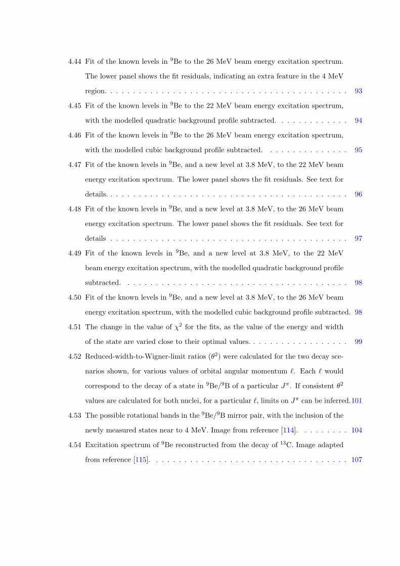
4.53 The possible rotational bands in the 9Be/9B mirror pair, with the inclusion of the

newly measured states near to 4 MeV. Image from reference [114]. . . . . . . . . 104

4.54 Excitation spectrum of 9Be reconstructed from the decay of 13C. Image adapted

from reference [115]. . . . . . . . . . . . . . . . . . . . . . . . . . . . . . . . . . . 107

5.1 Organic molecules: a) carbon tetrahedral bonds b) methane c) ethane. Various

carbon-carbon bonds: d) single bonding e) double bonding f) triple bonding.

Images adapted from reference [119]. . . . . . . . . . . . . . . . . . . . . . . . . . 111

5.2 The proposed nuclear reaction chain for Big Bang Nucleosynthesis. Image from

reference [122]. . . . . . . . . . . . . . . . . . . . . . . . . . . . . . . . . . . . . . 112

5.3 Triple-↵ process: The sequential capture of three ↵-particles to form 12C in its

ground state. . . . . . . . . . . . . . . . . . . . . . . . . . . . . . . . . . . . . . . 113

5.4 Schematic plot of a Gamow peak from reference [135] showing the contributions

from the Maxwell Boltzmann distribution of particle energies and the Coulomb

barrier tunnelling probability. . . . . . . . . . . . . . . . . . . . . . . . . . . . . . 115

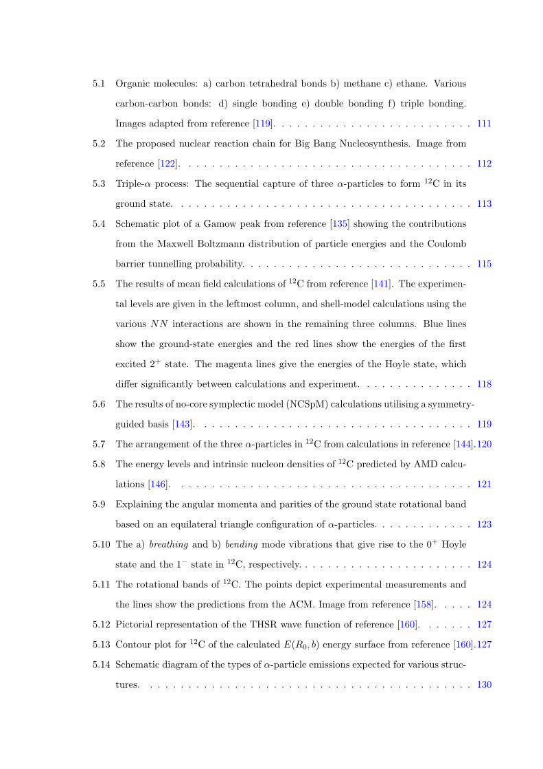
5.5 The results of mean field calculations of 12C from reference [141]. The experimen-

tal levels are given in the leftmost column, and shell-model calculations using the

various NN interactions are shown in the remaining three columns. Blue lines

show the ground-state energies and the red lines show the energies of the first

excited 2+ state. The magenta lines give the energies of the Hoyle state, which

di↵er significantly between calculations and experiment. . . . . . . . . . . . . . . 118

5.6 The results of no-core symplectic model (NCSpM) calculations utilising a symmetry-

guided basis [143]. . . . . . . . . . . . . . . . . . . . . . . . . . . . . . . . . . . . 119

5.7 The arrangement of the three ↵-particles in 12C from calculations in reference [144].120

5.8 The energy levels and intrinsic nucleon densities of 12C predicted by AMD calcu-

lations [146]. . . . . . . . . . . . . . . . . . . . . . . . . . . . . . . . . . . . . . . 121

5.9 Explaining the angular momenta and parities of the ground state rotational band

based on an equilateral triangle configuration of ↵-particles. . . . . . . . . . . . . 123

5.10 The a) breathing and b) bending mode vibrations that give rise to the 0+ Hoyle

state and the 1� state in 12C, respectively. . . . . . . . . . . . . . . . . . . . . . . 124

5.11 The rotational bands of 12C. The points depict experimental measurements and

the lines show the predictions from the ACM. Image from reference [158]. . . . . 124

5.12 Pictorial representation of the THSR wave function of reference [160]. . . . . . . 127

5.13 Contour plot for 12C of the calculated E(R0, b) energy surface from reference [160].127

5.14 Schematic diagram of the types of ↵-particle emissions expected for various struc-

tures. . . . . . . . . . . . . . . . . . . . . . . . . . . . . . . . . . . . . . . . . . . 130

5.15 The ratios of the adiabatic components of the Hoyle state (upper panel) and 0+3

resonance (lower panel) in 12C. The ratio of f2 to f3 varies during the decay of the

Hoyle state, but the f1 component remains dominant over all hyperradii. Here, E

is the energy above the ↵-particle decay threshold. Image from reference [176]. . 133

5.16 Various geometric configurations of a three-body decay. The situations are la-

belled from left to right as other collinear, extreme collinear and equal energies.

Other collinear: particles 1 and 2 remain close during the decay (similar to a

sequential decay). Extreme collinear: the decay is collinear and one particle re-

mains stationary. Equal energies: the particles are emitted with equal energies

and with equal angles between them. Image from reference [182]. . . . . . . . . . 135

5.17 The 8Be + ↵ Coulomb barrier as a function of the separation of the two fragments.137

5.18 The relative coordinates between the three particles in a direct decay. . . . . . . 138

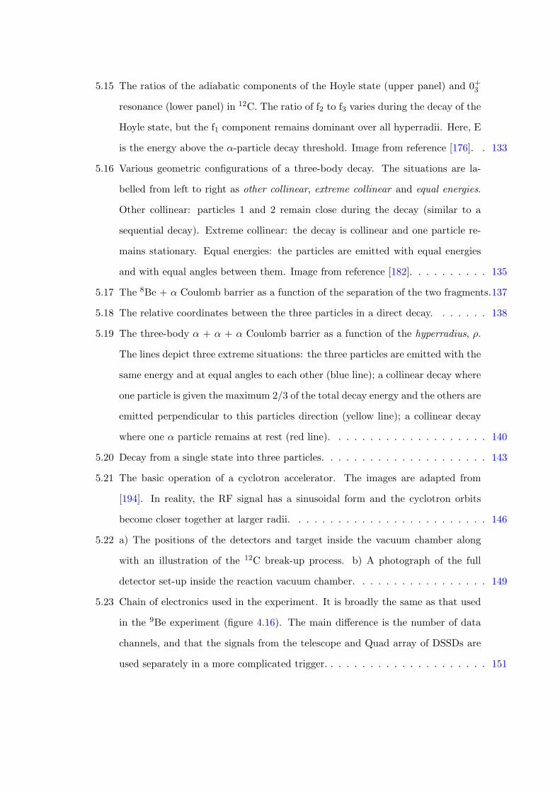
5.19 The three-body ↵ + ↵ + ↵ Coulomb barrier as a function of the hyperradius, ⇢.

The lines depict three extreme situations: the three particles are emitted with the

same energy and at equal angles to each other (blue line); a collinear decay where

one particle is given the maximum 2/3 of the total decay energy and the others are

emitted perpendicular to this particles direction (yellow line); a collinear decay

where one ↵ particle remains at rest (red line). . . . . . . . . . . . . . . . . . . . 140

5.20 Decay from a single state into three particles. . . . . . . . . . . . . . . . . . . . . 143

5.21 The basic operation of a cyclotron accelerator. The images are adapted from

[194]. In reality, the RF signal has a sinusoidal form and the cyclotron orbits

become closer together at larger radii. . . . . . . . . . . . . . . . . . . . . . . . . 146

5.22 a) The positions of the detectors and target inside the vacuum chamber along

with an illustration of the 12C break-up process. b) A photograph of the full

detector set-up inside the reaction vacuum chamber. . . . . . . . . . . . . . . . . 149

5.23 Chain of electronics used in the experiment. It is broadly the same as that used

in the 9Be experiment (figure 4.16). The main di↵erence is the number of data

channels, and that the signals from the telescope and Quad array of DSSDs are

used separately in a more complicated trigger. . . . . . . . . . . . . . . . . . . . . 151

5.24 Triggering circuit for the experiment. The aim was to demand three hits in the

quad arrangement of DSSDs, in coincidence with a single hit in the �E � E

telescope. In addition to triggering, the or outputs from the discriminators were

input to the TDC. . . . . . . . . . . . . . . . . . . . . . . . . . . . . . . . . . . . 152

5.25 Plot of the total Hoyle state peak-to-background ratio for the 12C excitation

spectrum (see figure 5.36 later for a spectrum). Extrapolating to zero beam

current does not give zero background. Therefore, a small background source,

around 1/3 of the amount at 6 enA beam energy, remains. . . . . . . . . . . . . . 155

5.26 Figure relating to table 5.1. Illustrating how the deduced hit position of two

particles changes if the energies detected by the front and rear strips change

order between the two particles, ↵ and �. Panels: a) The correct hit positions;

b) If the rear energies become switched; c) if the front energies become switched;

d) If front and rear energies become switched. . . . . . . . . . . . . . . . . . . . . 157

5.27 a) A total of seven Gaussian peaks fitted to a raw ↵-particle calibration spectrum

from a single detector channel. b) A plot of peak centroid vs ↵-particle energy. . 159

5.28 a) Schematic diagram of the set-up used to measure the energy losses of the

calibration ↵-particles in the source. b) A plot of the average ↵ energy vs. the

angle of emission from the source. The points show experimental data and the

line shows the Bethe formula prediction for 4He ions travelling through a 0.55 µm-

thick even mixture of 239Pu, 241Am and 244Cu. To obtain plot b), the detector

strips were calibrated in energy at zero degrees, since this is where the energy

losses are minimal. The calculations assumed a linear energy loss through the

source material, which causes the disagreement between the experimental data

and the Bethe formula prediction at large angles. . . . . . . . . . . . . . . . . . . 161

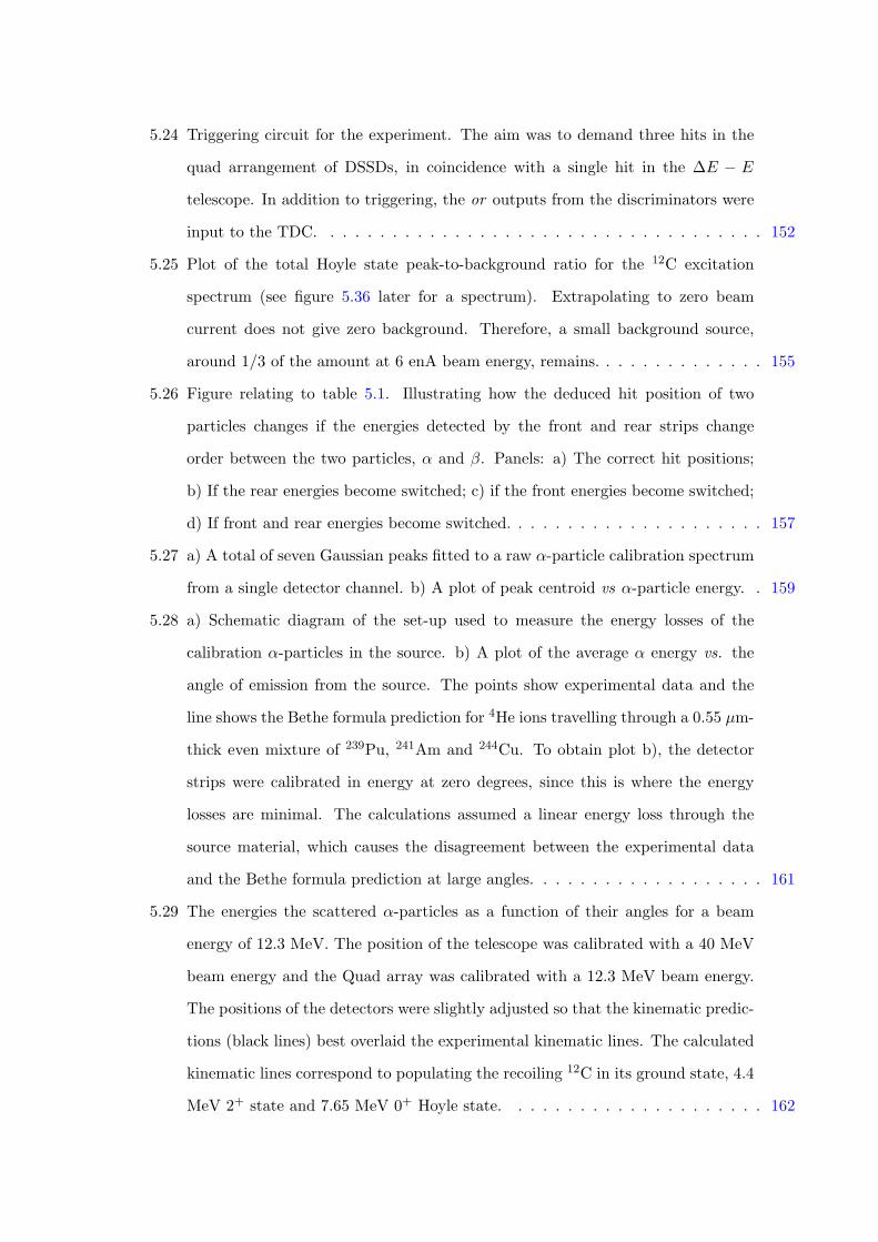
5.29 The energies the scattered ↵-particles as a function of their angles for a beam

energy of 12.3 MeV. The position of the telescope was calibrated with a 40 MeV

beam energy and the Quad array was calibrated with a 12.3 MeV beam energy.

The positions of the detectors were slightly adjusted so that the kinematic predic-

tions (black lines) best overlaid the experimental kinematic lines. The calculated

kinematic lines correspond to populating the recoiling 12C in its ground state, 4.4

MeV 2+ state and 7.65 MeV 0+ Hoyle state. . . . . . . . . . . . . . . . . . . . . 162

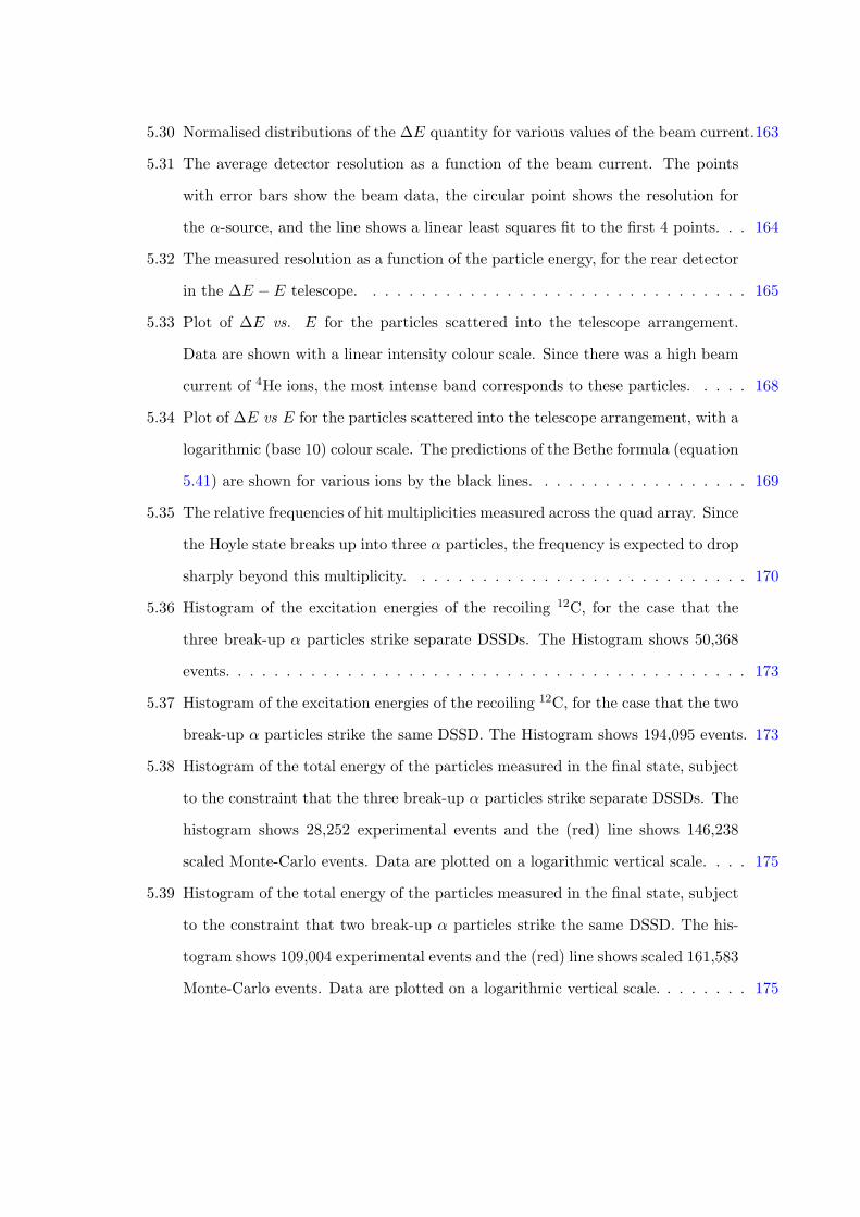
5.30 Normalised distributions of the �E quantity for various values of the beam current.163

5.31 The average detector resolution as a function of the beam current. The points

with error bars show the beam data, the circular point shows the resolution for

the ↵-source, and the line shows a linear least squares fit to the first 4 points. . . 164

5.32 The measured resolution as a function of the particle energy, for the rear detector

in the �E � E telescope. . . . . . . . . . . . . . . . . . . . . . . . . . . . . . . . 165

5.33 Plot of �E vs. E for the particles scattered into the telescope arrangement.

Data are shown with a linear intensity colour scale. Since there was a high beam

current of 4He ions, the most intense band corresponds to these particles. . . . . 168

5.34 Plot of �E vs E for the particles scattered into the telescope arrangement, with a

logarithmic (base 10) colour scale. The predictions of the Bethe formula (equation

5.41) are shown for various ions by the black lines. . . . . . . . . . . . . . . . . . 169

5.35 The relative frequencies of hit multiplicities measured across the quad array. Since

the Hoyle state breaks up into three ↵ particles, the frequency is expected to drop

sharply beyond this multiplicity. . . . . . . . . . . . . . . . . . . . . . . . . . . . 170

5.36 Histogram of the excitation energies of the recoiling 12C, for the case that the

three break-up ↵ particles strike separate DSSDs. The Histogram shows 50,368

events. . . . . . . . . . . . . . . . . . . . . . . . . . . . . . . . . . . . . . . . . . . 173

5.37 Histogram of the excitation energies of the recoiling 12C, for the case that the two

break-up ↵ particles strike the same DSSD. The Histogram shows 194,095 events. 173

5.38 Histogram of the total energy of the particles measured in the final state, subject

to the constraint that the three break-up ↵ particles strike separate DSSDs. The

histogram shows 28,252 experimental events and the (red) line shows 146,238

scaled Monte-Carlo events. Data are plotted on a logarithmic vertical scale. . . . 175

5.39 Histogram of the total energy of the particles measured in the final state, subject

to the constraint that two break-up ↵ particles strike the same DSSD. The his-

togram shows 109,004 experimental events and the (red) line shows scaled 161,583

Monte-Carlo events. Data are plotted on a logarithmic vertical scale. . . . . . . . 175

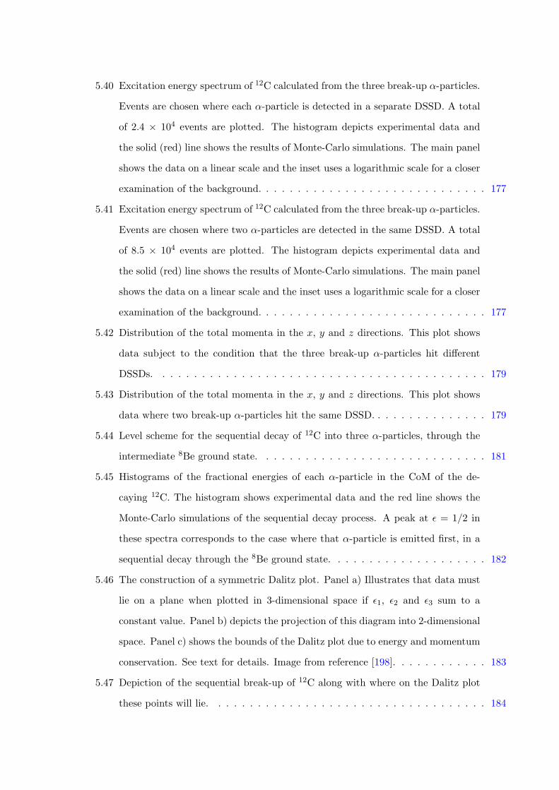
5.40 Excitation energy spectrum of 12C calculated from the three break-up ↵-particles.

Events are chosen where each ↵-particle is detected in a separate DSSD. A total

of 2.4 ⇥ 104 events are plotted. The histogram depicts experimental data and

the solid (red) line shows the results of Monte-Carlo simulations. The main panel

shows the data on a linear scale and the inset uses a logarithmic scale for a closer

examination of the background. . . . . . . . . . . . . . . . . . . . . . . . . . . . . 177

5.41 Excitation energy spectrum of 12C calculated from the three break-up ↵-particles.

Events are chosen where two ↵-particles are detected in the same DSSD. A total

of 8.5 ⇥ 104 events are plotted. The histogram depicts experimental data and

the solid (red) line shows the results of Monte-Carlo simulations. The main panel

shows the data on a linear scale and the inset uses a logarithmic scale for a closer

examination of the background. . . . . . . . . . . . . . . . . . . . . . . . . . . . . 177

5.42 Distribution of the total momenta in the x, y and z directions. This plot shows

data subject to the condition that the three break-up ↵-particles hit di↵erent

DSSDs. . . . . . . . . . . . . . . . . . . . . . . . . . . . . . . . . . . . . . . . . . 179

5.43 Distribution of the total momenta in the x, y and z directions. This plot shows

data where two break-up ↵-particles hit the same DSSD. . . . . . . . . . . . . . . 179

5.44 Level scheme for the sequential decay of 12C into three ↵-particles, through the

intermediate 8Be ground state. . . . . . . . . . . . . . . . . . . . . . . . . . . . . 181

5.45 Histograms of the fractional energies of each ↵-particle in the CoM of the de-

caying 12C. The histogram shows experimental data and the red line shows the

Monte-Carlo simulations of the sequential decay process. A peak at ✏ = 1/2 in

these spectra corresponds to the case where that ↵-particle is emitted first, in a

sequential decay through the 8Be ground state. . . . . . . . . . . . . . . . . . . . 182

5.46 The construction of a symmetric Dalitz plot. Panel a) Illustrates that data must

lie on a plane when plotted in 3-dimensional space if ✏1, ✏2 and ✏3 sum to a

constant value. Panel b) depicts the projection of this diagram into 2-dimensional

space. Panel c) shows the bounds of the Dalitz plot due to energy and momentum

conservation. See text for details. Image from reference [198]. . . . . . . . . . . . 183

5.47 Depiction of the sequential break-up of 12C along with where on the Dalitz plot

these points will lie. . . . . . . . . . . . . . . . . . . . . . . . . . . . . . . . . . . 184

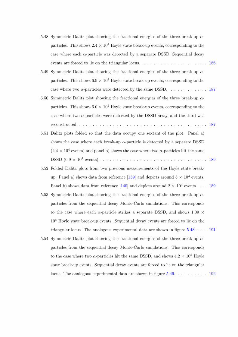
5.48 Symmetric Dalitz plot showing the fractional energies of the three break-up ↵-

particles. This shows 2.4 ⇥ 104 Hoyle state break-up events, corresponding to the

case where each ↵-particle was detected by a separate DSSD. Sequential decay

events are forced to lie on the triangular locus. . . . . . . . . . . . . . . . . . . . 186

5.49 Symmetric Dalitz plot showing the fractional energies of the three break-up ↵-

particles. This shows 6.9 ⇥ 104 Hoyle state break-up events, corresponding to the

case where two ↵-particles were detected by the same DSSD. . . . . . . . . . . . 187

5.50 Symmetric Dalitz plot showing the fractional energies of the three break-up ↵-

particles. This shows 6.0 ⇥ 104 Hoyle state break-up events, corresponding to the

case where two ↵-particles were detected by the DSSD array, and the third was

reconstructed. . . . . . . . . . . . . . . . . . . . . . . . . . . . . . . . . . . . . . . 187

5.51 Dalitz plots folded so that the data occupy one sextant of the plot. Panel a)

shows the case where each break-up ↵-particle is detected by a separate DSSD

(2.4 ⇥ 104 events) and panel b) shows the case where two ↵-particles hit the same

DSSD (6.9 ⇥ 104 events). . . . . . . . . . . . . . . . . . . . . . . . . . . . . . . . 189

5.52 Folded Dalitz plots from two previous measurements of the Hoyle state break-

up. Panel a) shows data from reference [139] and depicts around 5 ⇥ 103 events.

Panel b) shows data from reference [140] and depicts around 2 ⇥ 104 events. . . 189

5.53 Symmetric Dalitz plot showing the fractional energies of the three break-up ↵-

particles from the sequential decay Monte-Carlo simulations. This corresponds

to the case where each ↵-particle strikes a separate DSSD, and shows 1.09 ⇥105 Hoyle state break-up events. Sequential decay events are forced to lie on the

triangular locus. The analogous experimental data are shown in figure 5.48. . . . 191

5.54 Symmetric Dalitz plot showing the fractional energies of the three break-up ↵-

particles from the sequential decay Monte-Carlo simulations. This corresponds

to the case where two ↵-particles hit the same DSSD, and shows 4.2 ⇥ 105 Hoyle

state break-up events. Sequential decay events are forced to lie on the triangular

locus. The analogous experimental data are shown in figure 5.49. . . . . . . . . . 192

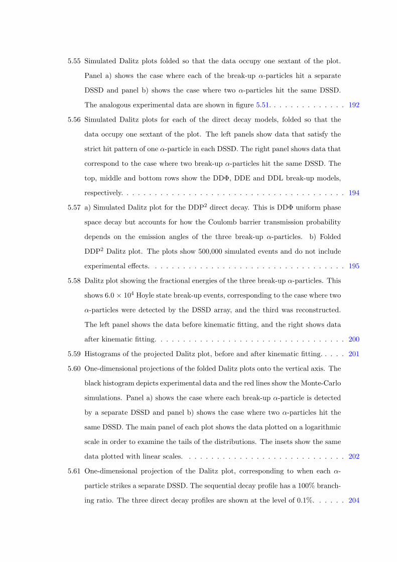
5.55 Simulated Dalitz plots folded so that the data occupy one sextant of the plot.

Panel a) shows the case where each of the break-up ↵-particles hit a separate

DSSD and panel b) shows the case where two ↵-particles hit the same DSSD.

The analogous experimental data are shown in figure 5.51. . . . . . . . . . . . . . 192

5.56 Simulated Dalitz plots for each of the direct decay models, folded so that the

data occupy one sextant of the plot. The left panels show data that satisfy the

strict hit pattern of one ↵-particle in each DSSD. The right panel shows data that

correspond to the case where two break-up ↵-particles hit the same DSSD. The

top, middle and bottom rows show the DD�, DDE and DDL break-up models,

respectively. . . . . . . . . . . . . . . . . . . . . . . . . . . . . . . . . . . . . . . . 194

5.57 a) Simulated Dalitz plot for the DDP2 direct decay. This is DD� uniform phase

space decay but accounts for how the Coulomb barrier transmission probability

depends on the emission angles of the three break-up ↵-particles. b) Folded

DDP2 Dalitz plot. The plots show 500,000 simulated events and do not include

experimental e↵ects. . . . . . . . . . . . . . . . . . . . . . . . . . . . . . . . . . . 195

5.58 Dalitz plot showing the fractional energies of the three break-up ↵-particles. This

shows 6.0 ⇥ 104 Hoyle state break-up events, corresponding to the case where two

↵-particles were detected by the DSSD array, and the third was reconstructed.

The left panel shows the data before kinematic fitting, and the right shows data

after kinematic fitting. . . . . . . . . . . . . . . . . . . . . . . . . . . . . . . . . . 200

5.59 Histograms of the projected Dalitz plot, before and after kinematic fitting. . . . . 201

5.60 One-dimensional projections of the folded Dalitz plots onto the vertical axis. The

black histogram depicts experimental data and the red lines show the Monte-Carlo

simulations. Panel a) shows the case where each break-up ↵-particle is detected

by a separate DSSD and panel b) shows the case where two ↵-particles hit the

same DSSD. The main panel of each plot shows the data plotted on a logarithmic

scale in order to examine the tails of the distributions. The insets show the same

data plotted with linear scales. . . . . . . . . . . . . . . . . . . . . . . . . . . . . 202

5.61 One-dimensional projection of the Dalitz plot, corresponding to when each ↵-

particle strikes a separate DSSD. The sequential decay profile has a 100% branch-

ing ratio. The three direct decay profiles are shown at the level of 0.1%. . . . . . 204

5.62 One-dimensional projection of the Dalitz plot, corresponding to where two ↵-

particles strike the same DSSD. The sequential decay profile has a 100% branching

ratio. The three direct decay profiles are shown at the level of 0.1%. . . . . . . . 204

5.63 The normalised likelihood of reproducing the experimental data as a function of

the direct decay branching ratio parameter. The dashed line shows the distri-

bution for a DDE/DDP2 direct decay contribution and the solid line shows the

distribution for the DD� decay. The likelihood distribution for the DDL decay

was much narrower and could not be plotted on the same scale. Upper limits on

the direct decay contributions were calculated by evaluating the 95% confidence

intervals of these distributions (P-value = 0.05), and are marked by the vertical

lines. . . . . . . . . . . . . . . . . . . . . . . . . . . . . . . . . . . . . . . . . . . . 206

5.64 DD� direct decay mechanism: Fit of Monte-Carlo simulations to the experimental

data for DD� branching ratios 0% (solid blue line), 0.047% (dot-dashed red line)

and 0.1% (dotted black line). . . . . . . . . . . . . . . . . . . . . . . . . . . . . . 207

5.65 DDE/DDP2 direct decay mechanism: Fit of Monte-Carlo simulations to the ex-

perimental data for DDE/DDP2 branching ratios 0% (solid blue line), 0.035%

(dot-dashed red line) and 0.1% (dotted black line). . . . . . . . . . . . . . . . . . 208

5.66 DDL direct decay mechanism: Fit of Monte-Carlo simulations to the experimental

data for DDL branching ratios 0% (solid blue line), 0.02% (dot-dashed red line)

and 0.1% (dotted black line). . . . . . . . . . . . . . . . . . . . . . . . . . . . . . 208

5.67 Three prior distributions chosen to reflect the present experimental knowledge

about the direct decay branching ratio. The vertical line marks the known upper

limit on the branching ratio (2� confidence) from reference [140]. . . . . . . . . . 213

5.68 A O-TPC image of the 12C(�,↵)8Be reaction from reference [203]. . . . . . . . . 218

B.1 Diagram showing the notation for the various parameters used to calculate the

detection angles of the particles. . . . . . . . . . . . . . . . . . . . . . . . . . . . 247

B.2 Diagram showing the horizontal and vertical angles required to fully label the

position of a particle detection within the detector array with respect to the

initial beam direction. . . . . . . . . . . . . . . . . . . . . . . . . . . . . . . . . . 247

C.1 Diagram used when deriving the form of the kinematic lines for two-body scattering.249

D.1 Diagrams used in deriving the Dalitz plot coordinates X and Y from the three

fractional energies ✏i. . . . . . . . . . . . . . . . . . . . . . . . . . . . . . . . . . . 251

D.2 The general bounds of the Dalitz plot, due to energy and momentum conservation,

for the case of unequal masses. Image adapted from reference [198]. . . . . . . . 255

E.1 The distribution of particle energies before (clear histogram) and after (filled

histogram) the kinematic fitting was performed, using one constraint equation.

The plot is layered such that the distribution after kinematic fitting can be seen

through the initial distribution. The uncertainty on each of the measured energies

decreases after the fit was performed, illustrated by the narrower distribution of

energies. . . . . . . . . . . . . . . . . . . . . . . . . . . . . . . . . . . . . . . . . . 257

E.2 The distribution of particle energies before (clear histogram) and after (filled

histogram) the kinematic fitting was performed, using both constraint equations.

The uncertainty on each of the measured energies decreases further when the

second constraint equation is applied. . . . . . . . . . . . . . . . . . . . . . . . . 258

E.3 The e↵ects of kinematic fitting (single constraint) when E2 (centre peak) is subject

to a systematic o↵set from its true value. The initial distribution is centred

on 10 MeV, rather than 9 MeV. The kinematic fitting procedure brings the E2

distribution closer to its true value of 9 MeV, but the other two quantities move

further from their true values. . . . . . . . . . . . . . . . . . . . . . . . . . . . . . 259

E.4 The e↵ects of kinematic fitting (both constraints) when E2 (centre peak) is subject

to a systematic o↵set from its true value. The kinematic fitting procedure brings

the E2 distribution closer to its true value of 9 MeV, and since the system is now

better-constrained, the other two parameters do not move far from their true values.259

E.5 The e↵ects of kinematic fitting (single constraint) when E2 (centre peak) is subject

to a systematic o↵set from its true value, but has a significantly larger statistical

uncertainty than the other parameters, (�1, �2, �3) = (0.5, 1.5, 0.5) MeV. . . . . 260

List of Tables

4.1 Comparison of 9B and 9Be experimental levels [52]. The horizontal lines high-

light a newly-measured state in 9B, which could correspond to the ⇡-antibinding

molecular configuration. 1 Tentative assignment from reference [65]. 2 Weighted

average of references [65, 66]. . . . . . . . . . . . . . . . . . . . . . . . . . . . . . 42

4.2 Calculation of ✓2 = �2/�2w for the 8Beg.s. + n/p decay channel of the 5/2�1 state. 102

4.3 The reduced-width-to-Wigner-limit ratios (8Beg.s.+n/p channel) for the 3.9 MeV

state in 9B and the 3.8 MeV state in 9Be for various values of the branching ratio. 103

5.1 Illustration of the mis-assignment of hit positions of particles on the same DSSD.

Particles ↵ and � have simulated energies E. They each deposit a signal in a

front and back strip. The energy orders of the two front, or two back strips that

fire are given by ord. f and ord. b. The front and rear strip energies are smeared

by �Ef and �Eb to give new energies E0f and E0

b. These may have a new energy

order (ord. f and ord. b). If this is the case, their hit positioned are switched

horizontally, vertically, or both. Rows separated by horizontal lines from top to

bottom are depicted in figure 5.26 panels a) � d). . . . . . . . . . . . . . . . . . 156

5.2 Comparing the number of generated Monte-Carlo events N , with the number

that reach the final Dalitz plots i. This provides a measure of the experimental

e�ciency ✏. Separate results are shown for the cases where each ↵-particle hits a

separate DSSD (hit pattern 1) and where two hit the same DSSD (hit pattern 2). 193

5.3 The values of branching ratio upper limits for each of the direct decay mechanisms.206

5.4 The values of the DD� branching ratio limits to 95% and 99.5% credible intervals

based on the Bayesian analysis. Uncertainties are systematic due to the choice of

prior. . . . . . . . . . . . . . . . . . . . . . . . . . . . . . . . . . . . . . . . . . . . 214

5.5 The values of branching ratio upper limits for each of the direct decay mechanisms.

The left columns of data correspond to the frequentist analysis and the right

columns correspond to the Bayesian analysis. The quoted systematic uncertainties

are due to the choice of prior distribution in the Bayesian analysis. . . . . . . . . 215

Chapter 1

Introduction

“Begin at the beginning,” the King said gravely,

“and go on till you come to the end: then stop.”

– Lewis Carroll, Alice in Wonderland

Atomic nuclei are self-bound objects that lie at the heart of every atom. Atoms have a size

around 1 A(10�10 m), whereas the atomic nucleus is 100,000 times smaller around 1 fm (10�15

m). Within nuclei, sub-atomic particles called nucleons can move both independently of each

other and collectively, giving rise to varied and interesting excitations of these systems.

To a nuclear physicist, these nucleons, called protons and neutrons, are the building blocks

of atomic nuclei. From more fundamental studies in particle physics, it is known that nucleons

are composite systems, consisting of quarks and gluons. A proton consists of uud quarks and a

neutron has an udd quark composition. However, to excite a proton (rest mass ⇡938 MeV/c2)

into an excited �+ state (rest mass ⇡1232 MeV/c2) takes several hundred MeV of energy. In

contrast, a typical nuclear excitation, based on the relative motion of the constituent nucleons,

typically occurs over an energy range of 0.1�10 MeV. Therefore, in low-energy nuclear physics,

protons and neutrons are treated as fundamental particles whose properties and interactions

give rise to observed nuclear properties.

1

Despite their small size, nuclei carry > 99% of the mass of the atom, so possess an incredibly

high average density around 2 ⇥ 1017 kg/m3. At the same time, they are also extremely dynamic

objects. A quantum mechanical particle such as a nucleon, trapped in a small, ⇡fm sized, space

such as a nucleus, must have a high momentum, due to Heisenberg’s position-momentum uncer-

tainty principle. In some cases, the motion of individual nucleons may amount to an appreciable

fraction of the speed of light. In this sense, atomic nuclei are incredibly exciting entities, far

removed from the macroscopic objects in the world around us. Some nuclei are spherical in

shape, but others possess a variety of interesting deformations and structures, which can rotate

like nuclear spinning-tops.

One of the most fundamental problems in nuclear physics is understanding the exact nature

of the nuclear force, which binds the nucleus together [1]. Much progress has been made in fun-

damental physics to understand the strong interaction between quarks and gluons, which will

underpin the residual nuclear force between nucleons. At incredibly high energies (TeV) and

densities, perturbation theory may successfully be applied to the strong interaction, due to the

behaviour of the strong coupling constant with energy [2]. At lower energies, recent advances in

chiral e↵ective field theory have provided a way to realistically model the interactions between

nucleons. Through ab initio calculations, where the various interactions between all constituent

nucleons are considered, many properties of light nuclei have been successfully calculated with

these realistic nucleon-nucleon interactions [3].

Due to the computationally intensive nature of calculating the properties of a many-body

system ab initio, part of the work of a nuclear physicist is to extract simpler descriptions of

nuclear systems. Therefore, a key feature in the study of nuclear physics is the application

of phenomenological models as a way of understanding observed phenomena [4]. Within each

description, the ability to interpret experimental data and make predictions based on the var-

ious phenomenological models is often fairly complete. However, nuclear physics does lack an

overriding theoretical formulation that would allow the analysis of all measured phenomena in

a consistent way.

2

One phenomenon that may add a great deal to our understanding of nuclear structure is the

idea of nuclear clustering. Clustering is the concept that groups of nucleons may preferentially

form in the nucleus, organising themselves into coherent crystal-like structures. The A-nucleon

many-body problem may then reduce down to a smaller configuration space where the e↵ective

interactions between clusters of nucleons need only be considered. The subject of clustering is

by no means a new idea, and has been discussed throughout the history of nuclear physics [5,

6]. Clustering is a recurrent feature, especially in light nuclei, and there are many documented

cases. In relation to this thesis, 9Be is thought to have an ↵ + n + ↵ molecular structure, where

the two ↵-particles are bound together through the exchange of the neutron. Furthermore, 12C

is well-described by the relative motion of three interacting ↵-particles.

Despite the experimental and theoretical attention that nuclear clustering has attracted, the

mechanism of cluster formation is not properly understood. Some studies have proposed that

the origin of clustering may be traced back to the depth of the confining nuclear potential, so

cluster formation should be a sensitive probe of the nuclear force [7]. Other questions arise

regarding to what extent the clusters maintain their identities in the nucleus. In 12C, for ex-

ample, the bosonic ↵-particles may form a Bose-Einstein-condensate-type state, if the fermonic

structures of the ↵-clusters can be ignored, e.g. in di↵use arrangements. The cluster structures

of various nuclei and their excited states are also predicted to have a significant role in stellar

nucleosynthesis, which plays a crucial part in the evolution of the universe. The present thesis

uses the experimental technique of break-up reactions in order to explore the potential cluster

structures of 9Be and 12C.

The following theory chapters describe some ways in which the nuclear many-body problem

has been simplified over the years and the progress that has been made towards understanding

the complex behaviour of atomic nuclei. The famous liquid-drop model and shell model are

initially discussed before a more in-depth discussion on nuclear deformation and clustering. The

basic theory of nuclear reactions is then covered before moving on to detailing three experiments.

The first explores the possible molecular structure of 9Be and the second answers the question

of whether the excited “Hoyle state” of 12C is an ↵-particle-condensate state. The third study

details improvements in the performance of resistive charge division strip detectors.

3

4

Chapter 2

Nuclear structure

2.1 The liquid drop model

An early attempt to understand the properties of atomic nuclei, by German physicist Carl

Friedrich von Weizsacker, was called the liquid drop model [8]. A nucleus has a constant binding

energy per nucleon, which is analogous to the latent heat of vaporisation of a fluid. Further-

more, surface tension e↵ects of a nucleus were thought to be similar to those of a liquid drop.

Therefore, by modelling the atomic nucleus as a liquid drop, a quantitative, empirical model

was developed that approximated the mass and binding energy of nuclei.

The latent heat of vaporisation of a fluid denotes the amount of energy required to convert

molecules from a liquid to a gas phase. Empirically, the latent heat of vaporisation was seen to

be proportional to the number of molecules making up the liquid (the total number of bonds)

[9]. In a similar way, the binding energy of a nucleus was also observed to be approximately

proportional to the total number of nucleons. Using this analogy, the semi-empirical mass for-

mula (SEMF) � known also as the Bethe-Weizacker formula � was derived.

In this liquid-drop picture, there are five terms that contribute to the binding energy of a

nucleus. The so-called volume term is directly proportional to the total number of nucleons, A,

as avA. Here, av is a proportionality constant, which is empirically-derived. This encapsulates

the idea that each nucleon in the nucleus interacts exclusively with its nearest neighbours, due

to the short-range nuclear interaction. The surface term accounts for the fact the nucleons on

5

the surface of the nucleus have fewer neighbouring nucleons compared with those in the nu-

clear interior. This term is analogous to formulation of the surface tension of a liquid drop.

Treating the nucleus as a sphere, if the volume is proportional to the total number of nucleons,

then the surface area is proportional to A2/3. Therefore, a reduction in the binding energy of

asA2/3 is expected. The Coulomb term accounts for the electrostatic repulsion between protons

in a nucleus, which does not only act between nearest neighbours. The electrostatic repulsion

between two protons is inversely proportional to their separation. Therefore, the average re-

duction in the binding energy in a nucleus with Z protons is acZ(Z�1)/A1/3. The Z(Z � 1), as

opposed to Z2, accounts for the fact that each proton can only interact with Z�1 other protons.

The final two terms are not analogous with a liquid drop and are exclusive to the quantum

mechanical nuclear system. The asymmetry term accounts for the di↵erence in the number

of protons and neutrons in the nucleus, aasym.(N�Z)2/A. This term corrects for the energy

associated with the Pauli exclusion principle, which states that two fermions can not occupy

exactly the same quantum state. Therefore, as more nucleons are added to the nucleus, they

must occupy higher energy levels, decreasing the overall binding energy. Since protons and

neutrons are distinct types of particles, they occupy di↵erent quantum states, meaning that

the lowest energy configuration corresponds to when there are equal numbers of each. The

final pairing term accounts for the spin-coupling e↵ects between like nucleons. The nucleus has

a lower energy when the number of “spin-up” protons/neutrons equals the number of “spin-

down” protons/neutrons. Only in the case where both Z and N are even, can this be the case

for both the protons and neutrons. This term takes the form ��/A1/2 where � changes value

between negative, zero, and positive, if the nucleus is even-even, even-odd or odd-odd. The total

semi-empirical mass formula is given by equation 2.1.

BE = avA� asA2/3 � acZ(Z�1)/A1/3 � aasym.(N�Z)2/A � �/A1/3 where, (2.1)

� ⇡ �12 MeV for even-even, 0 MeV for even-odd , +12 MeV for odd-odd . (2.2)

As shown in figure 2.1 a), when the parameters av through to aasym. are fit to the experi-

mentally measured binding energies, the general trend is successfully reproduced by the SEMF.

6

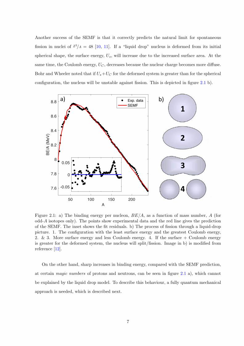
Another success of the SEMF is that it correctly predicts the natural limit for spontaneous

fission in nuclei of Z2/A = 48 [10, 11]. If a “liquid drop” nucleus is deformed from its initial

spherical shape, the surface energy, Us, will increase due to the increased surface area. At the

same time, the Coulomb energy, UC , decreases because the nuclear charge becomes more di↵use.

Bohr and Wheeler noted that if Us+UC for the deformed system is greater than for the spherical

configuration, the nucleus will be unstable against fission. This is depicted in figure 2.1 b).

50 100 150 200A

7.6

7.8

8

8.2

8.4

8.6

8.8

BE/A

(MeV

)

Exp. dataSEMF

a) b)1

2

3

450 100 150 200

A

-0.05

0

0.05

Res

idua

ls (M

eV)

Figure 2.1: a) The binding energy per nucleon, BE/A, as a function of mass number, A (forodd-A isotopes only). The points show experimental data and the red line gives the predictionof the SEMF. The inset shows the fit residuals. b) The process of fission through a liquid-droppicture. 1. The configuration with the least surface energy and the greatest Coulomb energy,2. & 3. More surface energy and less Coulomb energy. 4. If the surface + Coulomb energyis greater for the deformed system, the nucleus will split/fission. Image in b) is modified fromreference [12].

On the other hand, sharp increases in binding energy, compared with the SEMF prediction,

at certain magic numbers of protons and neutrons, can be seen in figure 2.1 a), which cannot

be explained by the liquid drop model. To describe this behaviour, a fully quantum mechanical

approach is needed, which is described next.

7

2.2 The spherical shell model

An electronic theory of the atom, based on the idea that electrons occupy a variety of single-

particle orbitals, has been very successful in describing the observed properties of atomic systems

[13]. In this atomic shell model, discrete single-particle levels are systematically filled in order of

energy, as dictated by the Pauli exclusion principle. In doing so, it is possible to obtain atomic

systems that consist of completely filled orbitals � closed shells � along with extra valence

electrons that lie beyond the closed shells. Under the assumption that the electrons contained

within the closed shells are inert, or non-interacting, the bulk of atomic properties can be un-

derstood by considering the motion and interactions of valence electrons alone. A key feature is

that, as more electrons are added to a system, moving left to right across the periodic table of

the elements, the observed properties vary smoothly. However, at certain numbers of electrons,

the properties of the atoms, such as their binding energies and radii, can be seen to undergo

an abrupt change. This corresponds to the case where an electronic shell has been filled. This

is analogous to the sudden increase in nuclear binding energies at certain magic numbers of

protons and neutrons.

Given the success of the atomic shell model, and the somewhat similar behaviour that atoms

and nuclei exhibit, it seems natural to apply a similar shell-model approach to atomic nuclei.

However, there are some major di↵erences between the two systems that make the nuclear sys-

tem more challenging to analyse in this manner. Foremost, the central Coulomb interaction set

up by the atomic nucleus, which forms the confining potential for the electrons in an atom, is

common between all of the electrons. On the other hand, nuclei are self-bound systems. Protons

and neutrons are bound together, without some central potential common to the whole system.

Secondly, atomic electrons interact with each other and the central potential by the Coulomb

interaction alone. The interaction between nucleons is far more complicated.

In the first half of the 20th century a breakthrough model was introduced to explain the

observed magic numbers in nuclei. The motion of individual nucleons was approximated to be

defined by a potential that is caused by the average interaction of a nucleon with each of the

other nucleons. This mean-field approach was named the spherical shell-model of the nucleus

8

[14]. Nucleon-nucleus scattering experiments indicated that the charge distribution of a nucleus

was fairly constant within the nuclear interior, with a di↵useness at the nuclear surface [15].

Assuming that the spatial variation of the nuclear interaction was proportional to the density

of nuclear matter throughout the nucleus, the confining potential was considered to follow a

Woods-Saxon profile [15] as

V (r) = � V0

1 + e(r�R0

)/a, (2.3)

where R0 is the nuclear radius (the point at which the nuclear density drops to 1/2 of its interior

value, and a is a di↵useness parameter, which dictates how sharply the nuclear density drops at

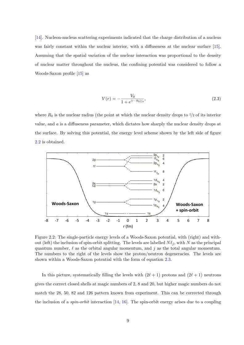
the surface. By solving this potential, the energy level scheme shown by the left side of figure

2.2 is obtained.

-8-7-6-5-4-3-2-1012345678r(fm)

Woods-Saxon Woods-Saxon+spin-orbit

Figure 2.2: The single-particle energy levels of a Woods-Saxon potential, with (right) and with-out (left) the inclusion of spin-orbit splitting. The levels are labelled N`j , with N as the principalquantum number, ` as the orbital angular momentum, and j as the total angular momentum.The numbers to the right of the levels show the proton/neutron degeneracies. The levels areshown within a Woods-Saxon potential with the form of equation 2.3.

In this picture, systematically filling the levels with (2` + 1) protons and (2` + 1) neutrons

gives the correct closed shells at magic numbers of 2, 8 and 20, but higher magic numbers do not

match the 28, 50, 82 and 126 pattern known from experiment. This can be corrected through

the inclusion of a spin-orbit interaction [14, 16]. The spin-orbit energy arises due to a coupling

9

between the intrinsic spin of the nucleons, s, and their orbital angular momentum, `, such that

the total angular momentum is defined by the vector sum j = `+ s. In atomic physics, there is

also a spin-orbit interaction for electrons due to the interaction between their magnetic moment

and the field generated due to their orbital motion in the atom. The nuclear spin-orbit interac-

tion has the same general form as for electrons, Vso(` · s), but cannot have an electromagnetic

origin, because its e↵ect is too strong.

Consider the states on the left side of figure 2.2. The ` = 1, 1p level has a total degeneracy

of 2(2`+ 1) = 6. Coupling this angular momentum to the nucleon spins gives possible j values

of `± 1/2 = 1/2 or 3/2. Since these two situations correspond to di↵erent alignments of the orbital

angular momentum and spin, the spin-orbit interaction energy ensures that they are no longer

degenerate in energy, i.e. the level splits. Due to the (` · s) nature of the interaction, the energy

splitting is greater for higher `. Inclusion of the spin-orbit term gives the energy levels on the

right hand side of figure 2.2 and generates the correct magic numbers.

Perhaps surprisingly, given the simplifications made during its formulation, this final shell-

model description is very powerful in predicting many properties of nuclei. For example, even-

even nuclei are always J⇡ = 0+ in their ground states, which is obtained when systematically

filling these shell-model levels. Here J is the total angular momentum of the nucleus and ⇡ is

the parity. Likewise, the levels structures of nuclei with one or two nucleons beyond a closed

shell can be successfully examined through an m-scheme angular momentum coupling. In cases

where there are a higher number of nucleons beyond a closed shell, the interactions between

them can no longer be ignored, and the interacting particle shell-model must be employed [17].

10

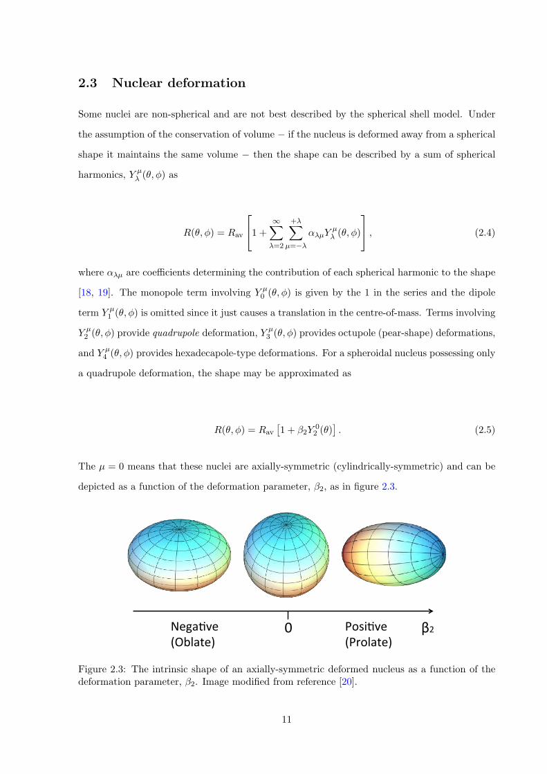
2.3 Nuclear deformation

Some nuclei are non-spherical and are not best described by the spherical shell model. Under

the assumption of the conservation of volume � if the nucleus is deformed away from a spherical

shape it maintains the same volume � then the shape can be described by a sum of spherical

harmonics, Y µ� (✓,�) as

R(✓,�) = Rav

2

41 +1X

�=2

+�X

µ=��

↵�µYµ� (✓,�)

3

5 , (2.4)

where ↵�µ are coe�cients determining the contribution of each spherical harmonic to the shape

[18, 19]. The monopole term involving Y µ0 (✓,�) is given by the 1 in the series and the dipole

term Y µ1 (✓,�) is omitted since it just causes a translation in the centre-of-mass. Terms involving

Y µ2 (✓,�) provide quadrupole deformation, Y µ

3 (✓,�) provides octupole (pear-shape) deformations,

and Y µ4 (✓,�) provides hexadecapole-type deformations. For a spheroidal nucleus possessing only

a quadrupole deformation, the shape may be approximated as

R(✓,�) = Rav

⇥1 + �2Y

02 (✓)

⇤. (2.5)

The µ = 0 means that these nuclei are axially-symmetric (cylindrically-symmetric) and can be

depicted as a function of the deformation parameter, �2, as in figure 2.3.

β20Nega)ve(Oblate)

Posi)ve(Prolate)

Figure 2.3: The intrinsic shape of an axially-symmetric deformed nucleus as a function of thedeformation parameter, �2. Image modified from reference [20].

11

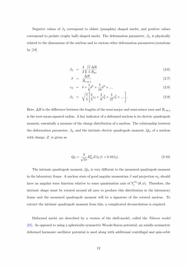
Negative values of �2 correspond to oblate (pumpkin) shaped nuclei, and positive values

correspond to prolate (rugby ball) shaped nuclei. The deformation parameter, �2, is physically

related to the dimensions of the nucleus and to various other deformation parameters/notations

by [19]

�2 =4

3

r⇡

5

�R

Rav(2.6)

� =�R

Rr.m.s(2.7)

✏2 = � +1

6�2 +

5

18�3 + .... (2.8)

�2 =

r⇡

5

"4

3✏2 +

4

9✏22 +

4

27✏32 + ....

#. (2.9)

Here, �R is the di↵erence between the lengths of the semi-major and semi-minor axes and Rr.m.s

is the root-mean-squared radius. A key indicator of a deformed nucleus is its electric quadrupole

moment, essentially a measure of the charge distribution of a nucleus. The relationship between

the deformation parameter, �2, and the intrinsic electric quadrupole moment, Q0, of a nucleus

with charge, Z, is given as

Q0 =3p5⇡

R2avZ�2 (1 + 0.16�2) . (2.10)

The intrinsic quadrupole moment, Q0, is very di↵erent to the measured quadrupole moment

in the laboratory frame. A nuclear state of good angular momentum J and projection mj should

have an angular wave function relative to some quantisation axis of Ymj

j (✓,�). Therefore, the

intrinsic shape must be rotated around all axes to produce this distribution in the laboratory

frame and the measured quadrupole moment will be a signature of the rotated nucleus. To

extract the intrinsic quadrupole moment from this, a complicated deconvolution is required.

Deformed nuclei are described by a version of the shell-model, called the Nilsson model

[21]. As opposed to using a spherically-symmetric Woods-Saxon potential, an axially-symmetric

deformed harmonic oscillator potential is used along with additional centrifugal and spin-orbit

12

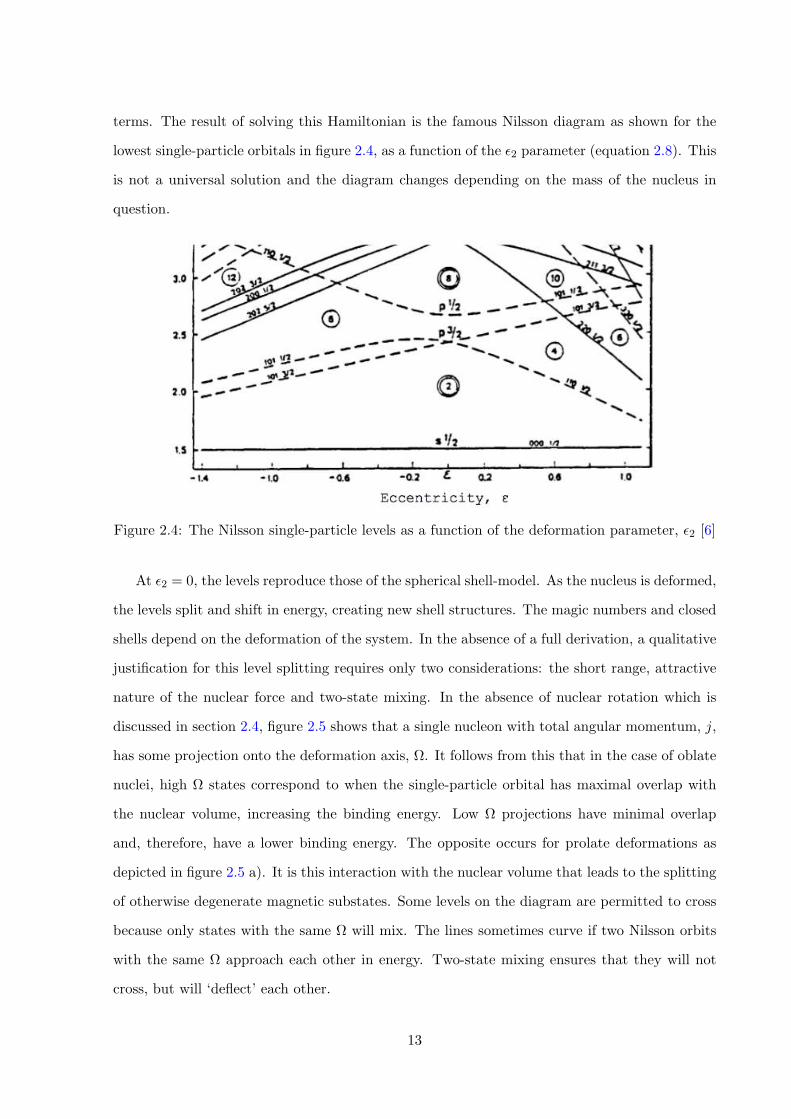
terms. The result of solving this Hamiltonian is the famous Nilsson diagram as shown for the

lowest single-particle orbitals in figure 2.4, as a function of the ✏2 parameter (equation 2.8). This

is not a universal solution and the diagram changes depending on the mass of the nucleus in

question.

Figure 2.4: The Nilsson single-particle levels as a function of the deformation parameter, ✏2 [6]

At ✏2 = 0, the levels reproduce those of the spherical shell-model. As the nucleus is deformed,

the levels split and shift in energy, creating new shell structures. The magic numbers and closed

shells depend on the deformation of the system. In the absence of a full derivation, a qualitative

justification for this level splitting requires only two considerations: the short range, attractive

nature of the nuclear force and two-state mixing. In the absence of nuclear rotation which is

discussed in section 2.4, figure 2.5 shows that a single nucleon with total angular momentum, j,

has some projection onto the deformation axis, ⌦. It follows from this that in the case of oblate

nuclei, high ⌦ states correspond to when the single-particle orbital has maximal overlap with

the nuclear volume, increasing the binding energy. Low ⌦ projections have minimal overlap

and, therefore, have a lower binding energy. The opposite occurs for prolate deformations as

depicted in figure 2.5 a). It is this interaction with the nuclear volume that leads to the splitting

of otherwise degenerate magnetic substates. Some levels on the diagram are permitted to cross

because only states with the same ⌦ will mix. The lines sometimes curve if two Nilsson orbits

with the same ⌦ approach each other in energy. Two-state mixing ensures that they will not

cross, but will ‘deflect’ each other.

13

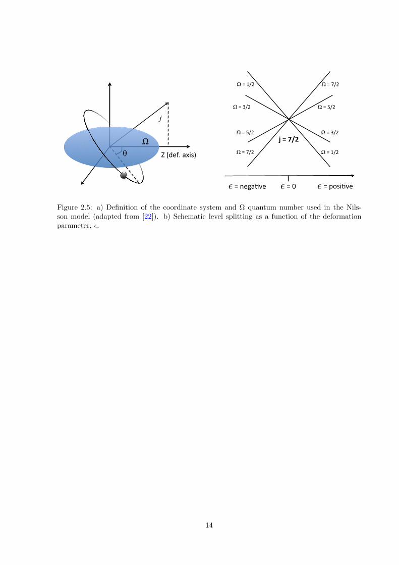
Z(def.axis)

j

Ω θ

j=7/2

Ω=7/2

Ω=5/2

Ω=3/2

Ω=1/2

Ω=1/2

Ω=3/2

Ω=5/2

Ω=7/2

ε=0 ε=posi/veε=nega/ve

Figure 2.5: a) Definition of the coordinate system and ⌦ quantum number used in the Nils-son model (adapted from [22]). b) Schematic level splitting as a function of the deformationparameter, ✏.

14

2.4 Collective rotation

Despite the successes of the spherical shell model and the deformed Nilsson model, to describe

a range of nuclei, the possibility of the collective motion of nucleons must also be considered.

In the shell-model picture, protons and neutrons systematically fill single-particle levels to form

the lowest (ground) state. In this picture, to form an excited state of a closed-shell even-even

nucleus, a pair of protons or neutrons must be broken and one promoted to a higher oscillator

shell. As such, the large shell-gap energy should mean that the first excited state is found at a

particularly high excitation energy. Additionally, this first excited state may have the opposite

parity to the ground state. In many cases, such behaviour is not observed. In fact, a key indi-

cator of collective behaviour in an even-even nucleus with a 0+ ground state, is the existence of

a relatively low-energy 2+ first excited state.

One form of collectivity, exclusive to deformed nuclei, is rotation. Since clustered nuclei are

inherently deformed and non-spherical, the experimental observation of rotation in these systems

is key evidence for the existence of clusters. Such rotational behaviour has also been observed in

many deformed poly-atomic molecular systems [23]. A deformed nucleus can generate angular

momentum collectively via rotation (or vibration) or by single-particle excitations in which

unpaired nucleons generate angular momentum. In practice, many states are a mixture of these

two cases. Firstly, consider the case of an inert, rotating nucleus, while ignoring the motion of

valence nucleons. In classical mechanics, the kinetic energy of a rotating object with a moment

of inertia, I, at an angular frequency of ! is given by

E(!) =1

2I!2. (2.11)

Since the angular momentum of an object is J = I!, the rotational kinetic energy can be

rewritten as E = J2/2I. Since a nucleus is a quantum mechanical object, the angular momentum

is replaced with the angular momentum operator cJ2, which has eigenvalues of h2J(J +1). This

gives a quantum mechanical rotational energy of

15

E(J) =h2

2I J (J + 1) . (2.12)

Therefore, the quantum mechanical energy levels of a rotating nucleus are proportional to

J(J + 1). By increasing the J quantum number, the excited states follow a pattern known as a

rotational band. By plotting the excitation energies of a rotating system against J(J +1) of the

levels, a linear relationship should be found. In some cases where nuclear rotation is built upon

an excited state, the band head, the lowest energy state in the band, lies at a higher excitation,

E0, than the ground state, hence, equation 2.12 becomes

E(J) = E0 +h2

2I J (J + 1) . (2.13)

In the case where the motion of valence nucleons within the rotating nucleus cannot be

ignored, the angular momentum coupling scheme of figure 2.6 must be considered. Here, the

total angular momentum of the nucleus, J , comes from several sources, not just the collective

rotation. The orbital angular momentum and spin of an individual nucleon, ` and s, couple to a

single-particle angular momentum of j . This has a projection onto the deformation (symmetry

axis) of ⌦. A rotating nucleus will also have a component, R, due to the collective rotation,

which will couple with j to give a total angular momentum of J , such that J =P

i j i + R.

The projection of J onto the deformation axis is denoted by K, and it is this quantity that

labels the rotational band. For most band heads, J = K =P

i⌦i, i.e. the angular momenta are

aligned along the deformation axis, because of something called collective back rotation. It can

be shown that, in order to minimise the rotational energy, the collective angular momentum of

the core is equal and opposite to the component of the single-particle angular momentum.

16

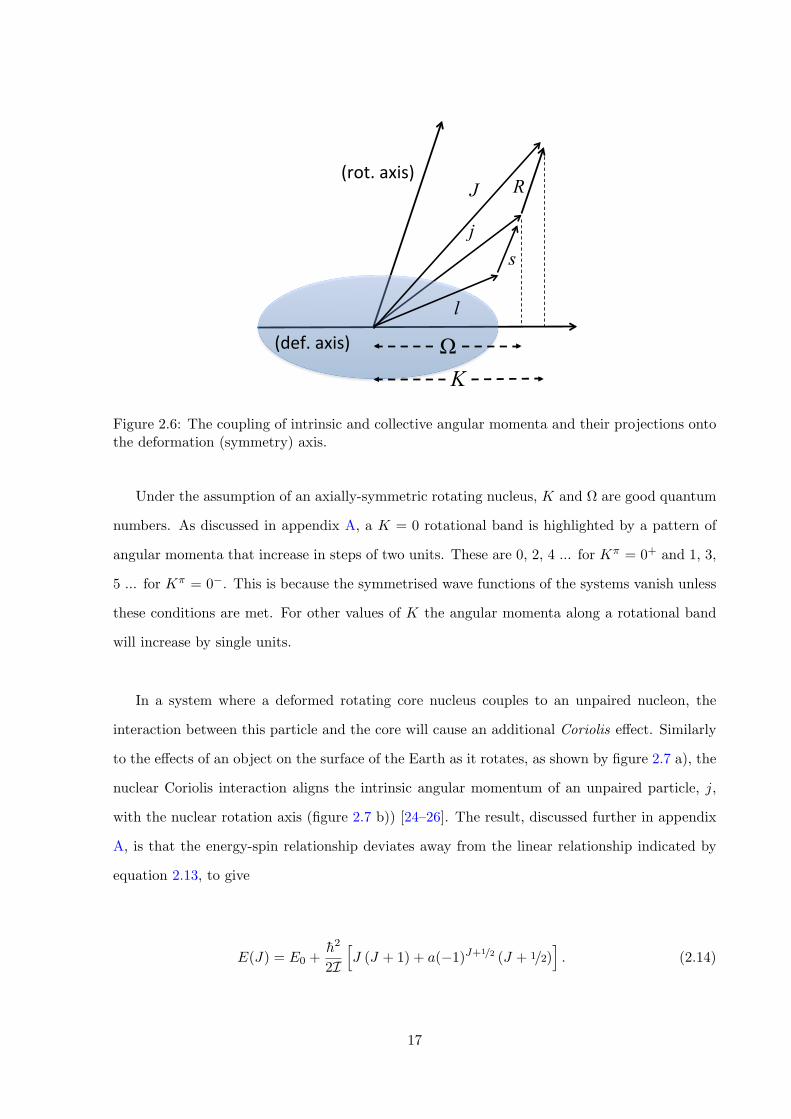
(def.axis)

j

Ω

l

s

R J

K

(rot.axis)

Figure 2.6: The coupling of intrinsic and collective angular momenta and their projections ontothe deformation (symmetry) axis.

Under the assumption of an axially-symmetric rotating nucleus, K and ⌦ are good quantum

numbers. As discussed in appendix A, a K = 0 rotational band is highlighted by a pattern of

angular momenta that increase in steps of two units. These are 0, 2, 4 ... for K⇡ = 0+ and 1, 3,

5 ... for K⇡ = 0�. This is because the symmetrised wave functions of the systems vanish unless

these conditions are met. For other values of K the angular momenta along a rotational band

will increase by single units.

In a system where a deformed rotating core nucleus couples to an unpaired nucleon, the

interaction between this particle and the core will cause an additional Coriolis e↵ect. Similarly

to the e↵ects of an object on the surface of the Earth as it rotates, as shown by figure 2.7 a), the

nuclear Coriolis interaction aligns the intrinsic angular momentum of an unpaired particle, j,

with the nuclear rotation axis (figure 2.7 b)) [24–26]. The result, discussed further in appendix

A, is that the energy-spin relationship deviates away from the linear relationship indicated by

equation 2.13, to give

E(J) = E0 +h2

2IhJ (J + 1) + a(�1)J+

1/2 (J + 1/2)i. (2.14)

17

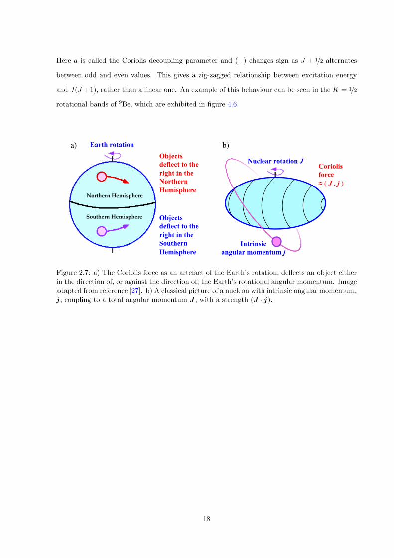
Here a is called the Coriolis decoupling parameter and (�) changes sign as J + 1/2 alternates

between odd and even values. This gives a zig-zagged relationship between excitation energy

and J(J +1), rather than a linear one. An example of this behaviour can be seen in the K = 1/2

rotational bands of 9Be, which are exhibited in figure 4.6.

Objects deflect to the right in the Northern Hemisphere

Objects deflect to the right in the Southern Hemisphere

Earth rotation

Nuclear rotation J

Intrinsic angular momentum j

Coriolis force ≈ ( J . j )

a) b)

Figure 2.7: a) The Coriolis force as an artefact of the Earth’s rotation, deflects an object eitherin the direction of, or against the direction of, the Earth’s rotational angular momentum. Imageadapted from reference [27]. b) A classical picture of a nucleon with intrinsic angular momentum,j , coupling to a total angular momentum J , with a strength (J · j ).

18

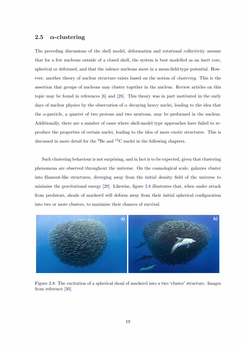
2.5 ↵-clustering

The preceding discussions of the shell model, deformation and rotational collectivity assume

that for a few nucleons outside of a closed shell, the system is best modelled as an inert core,

spherical or deformed, and that the valence nucleons move in a mean-field-type potential. How-

ever, another theory of nuclear structure exists based on the notion of clustering. This is the

assertion that groups of nucleons may cluster together in the nucleus. Review articles on this

topic may be found in references [6] and [28]. This theory was in part motivated in the early

days of nuclear physics by the observation of ↵ decaying heavy nuclei, leading to the idea that

the ↵-particle, a quartet of two protons and two neutrons, may be preformed in the nucleus.

Additionally, there are a number of cases where shell-model type approaches have failed to re-

produce the properties of certain nuclei, leading to the idea of more exotic structures. This is

discussed in more detail for the 9Be and 12C nuclei in the following chapters.

Such clustering behaviour is not surprising, and in fact is to be expected, given that clustering

phenomena are observed throughout the universe. On the cosmological scale, galaxies cluster

into filament-like structures, diverging away from the initial density field of the universe to

minimise the gravitational energy [29]. Likewise, figure 2.8 illustrates that, when under attack

from predators, shoals of mackerel will deform away from their initial spherical configuration

into two or more clusters, to maximise their chances of survival.

a) b)

Figure 2.8: The excitation of a spherical shoal of mackerel into a two ‘cluster’ structure. Imagesfrom reference [30].

19

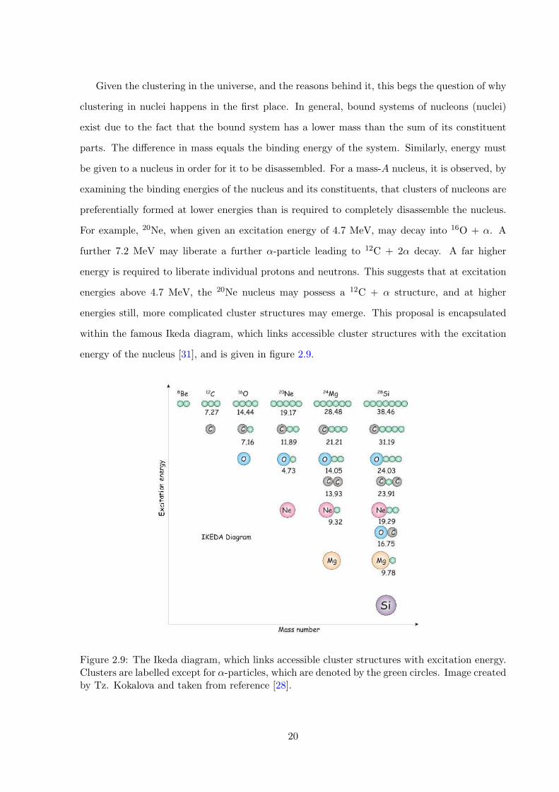
Given the clustering in the universe, and the reasons behind it, this begs the question of why

clustering in nuclei happens in the first place. In general, bound systems of nucleons (nuclei)

exist due to the fact that the bound system has a lower mass than the sum of its constituent

parts. The di↵erence in mass equals the binding energy of the system. Similarly, energy must

be given to a nucleus in order for it to be disassembled. For a mass-A nucleus, it is observed, by

examining the binding energies of the nucleus and its constituents, that clusters of nucleons are

preferentially formed at lower energies than is required to completely disassemble the nucleus.

For example, 20Ne, when given an excitation energy of 4.7 MeV, may decay into 16O + ↵. A

further 7.2 MeV may liberate a further ↵-particle leading to 12C + 2↵ decay. A far higher

energy is required to liberate individual protons and neutrons. This suggests that at excitation

energies above 4.7 MeV, the 20Ne nucleus may possess a 12C + ↵ structure, and at higher

energies still, more complicated cluster structures may emerge. This proposal is encapsulated

within the famous Ikeda diagram, which links accessible cluster structures with the excitation

energy of the nucleus [31], and is given in figure 2.9.

Figure 2.9: The Ikeda diagram, which links accessible cluster structures with excitation energy.Clusters are labelled except for ↵-particles, which are denoted by the green circles. Image createdby Tz. Kokalova and taken from reference [28].

20

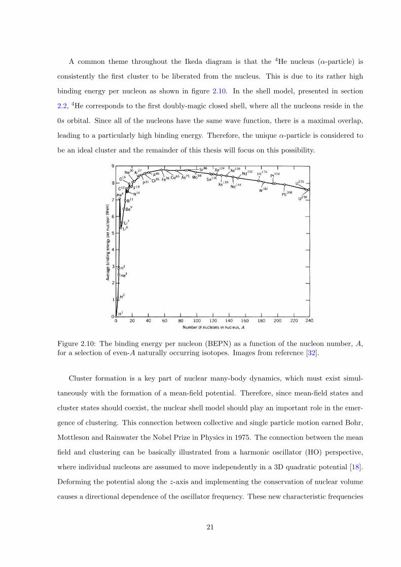
A common theme throughout the Ikeda diagram is that the 4He nucleus (↵-particle) is

consistently the first cluster to be liberated from the nucleus. This is due to its rather high

binding energy per nucleon as shown in figure 2.10. In the shell model, presented in section

2.2, 4He corresponds to the first doubly-magic closed shell, where all the nucleons reside in the

0s orbital. Since all of the nucleons have the same wave function, there is a maximal overlap,

leading to a particularly high binding energy. Therefore, the unique ↵-particle is considered to

be an ideal cluster and the remainder of this thesis will focus on this possibility.

Figure 2.10: The binding energy per nucleon (BEPN) as a function of the nucleon number, A,for a selection of even-A naturally occurring isotopes. Images from reference [32].

Cluster formation is a key part of nuclear many-body dynamics, which must exist simul-

taneously with the formation of a mean-field potential. Therefore, since mean-field states and

cluster states should coexist, the nuclear shell model should play an important role in the emer-

gence of clustering. This connection between collective and single particle motion earned Bohr,

Mottleson and Rainwater the Nobel Prize in Physics in 1975. The connection between the mean

field and clustering can be basically illustrated from a harmonic oscillator (HO) perspective,

where individual nucleons are assumed to move independently in a 3D quadratic potential [18].

Deforming the potential along the z-axis and implementing the conservation of nuclear volume

causes a directional dependence of the oscillator frequency. These new characteristic frequencies

21

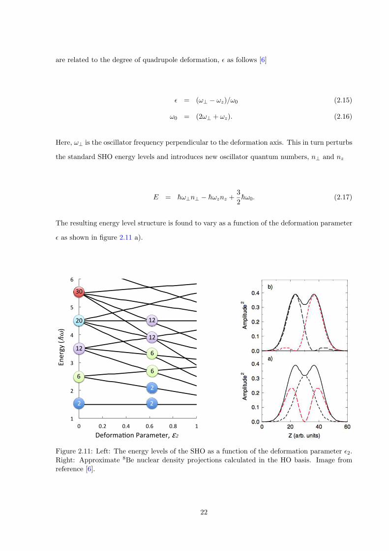
are related to the degree of quadrupole deformation, ✏ as follows [6]

✏ = (!? � !z)/!0 (2.15)

!0 = (2!? + !z). (2.16)

Here, !? is the oscillator frequency perpendicular to the deformation axis. This in turn perturbs

the standard SHO energy levels and introduces new oscillator quantum numbers, n? and nz

E = h!?n? � h!znz +3

2h!0. (2.17)

The resulting energy level structure is found to vary as a function of the deformation parameter

✏ as shown in figure 2.11 a).

1"

2"

3"

4"

5"

6"

0" 0.2" 0.4" 0.6" 0.8" 1"Deforma2on"Parameter,"ε2"

Energy"(ℏω)

"

2" 2"

2"

6"

6"

6"

12"

12"

12"20"

30"

Figure 2.11: Left: The energy levels of the SHO as a function of the deformation parameter ✏2.Right: Approximate 8Be nuclear density projections calculated in the HO basis. Image fromreference [6].

22

As expected, ✏ = 0 reproduces the standard HO levels. The key feature to note is the cross-

ing of the levels at a deformation of 2:1 (✏ = 0.63). The new degeneracies demonstrate that

the shell structure has evolved. At 2:1 deformation, the sequence of standard HO degenerate

levels are repeated twice, indicative of two interacting spherical HO potentials and suggestive

of clustering behaviour. These symmetries in the magic numbers emerge at additional defor-

mations of 3:1, 4:1 etc and establish a link between deformed shell closures and cluster formation.

Inspection of the densities of the nucleons that occupy the deformed orbitals provides further

indications of clustering. Consider the proposed 2↵ structure of 8Be, which would correspond to

a 2:1 deformation. The levels shown in figure 2.11 a) are systematically filled with 4 protons and 4

neutrons where pairs of particles couple to spin zero. The levels corresponding to [n?, nz] = [0, 0]

and [0, 1] are occupied and the corresponding 8Be density is given as |�0,0|2 + |�0,1|2. This has

previously been evaluated and is plotted as a function of distance along the deformation axis

in figure 2.11 b). A double-humped distribution is formed, indicative of a 2↵ cluster structure.

Furthermore, it has been calculated that the density distribution has a greater than 90% overlap

with the wave function of a free ↵-particle [33]. Clearly, the clustering that naturally emerges

acts to deform the mean field that produced it in the first place. Herein lies the problem with

a mean-field approach in the context of clustering.

Since each chapter of this thesis, relating to experimental studies of 9Be and 12C, gives

detailed theoretical introductions to clustering in each of these nuclei, any further theoretical

discussion of ↵-clustering is left until then. However, it is useful to consider what the experi-

mental signatures for ↵-clustered states may be. Since clustering indicates a departure from a

spherical shape, clustered nuclei will rotate, meaning that the discussion in section 2.4 is quite

pertinent. By examining the energy-spin systematics of states in a clustered nucleus, the nu-

clear moment of inertia may be extracted and inferences about its shape can be made. Further,

if the nuclear charge distribution deviates away from a spherical shape, the measured electric

quadrupole moment will be non-zero. Finally, if a nuclear state is clustered, then it is reason-

able to assume that when it decays, it will preferentially do so by emission of the cluster. To

fully understand this, the discussion of resonances and nuclear reactions in chapter 3 must be

considered.

23

Chapter 3

Nuclear reactions

3.1 Nuclear resonances

The aim of this thesis is to examine the excited states in 9Be and 12C in order to understand

elements of their structure. The nuclear states under investigation lie at su�ciently high energy

that they will preferentially choose to decay through particle emission, rather than electromag-

netic decays to the ground state. These states appear as resonances in the reaction cross section,

and their manifestation will depend on the reaction chosen to populate them, and the way in

which they decay. As such, a general discussion about nuclear resonances will be useful.

In the 1930’s, several experimental studies measured n +AZ X reactions, and by measuring

the resulting decay radioactivity of the sample, were able to assess the probability of neutron

absorption, or the reaction cross section [34, 35]. It was observed that the cross section was

strongly energy dependent, which led to the idea of unbound, long-lived states in the n +AZ X

system, at an energy defined by the centre-of-mass energy of the collision. A simple mathematical

form for the reaction cross section was derived by Breit and Wigner [36, 37] as

�(E) =⇤2

⇡S

�s�r(E � E0)2 + �2

, (3.1)

where ⇤ is the de Broglie wavelength of the projectile, E0 is the frequency of the resonance,

S = 2J + 1 (with J as the total angular momentum of the resonance), � is the total width of

25

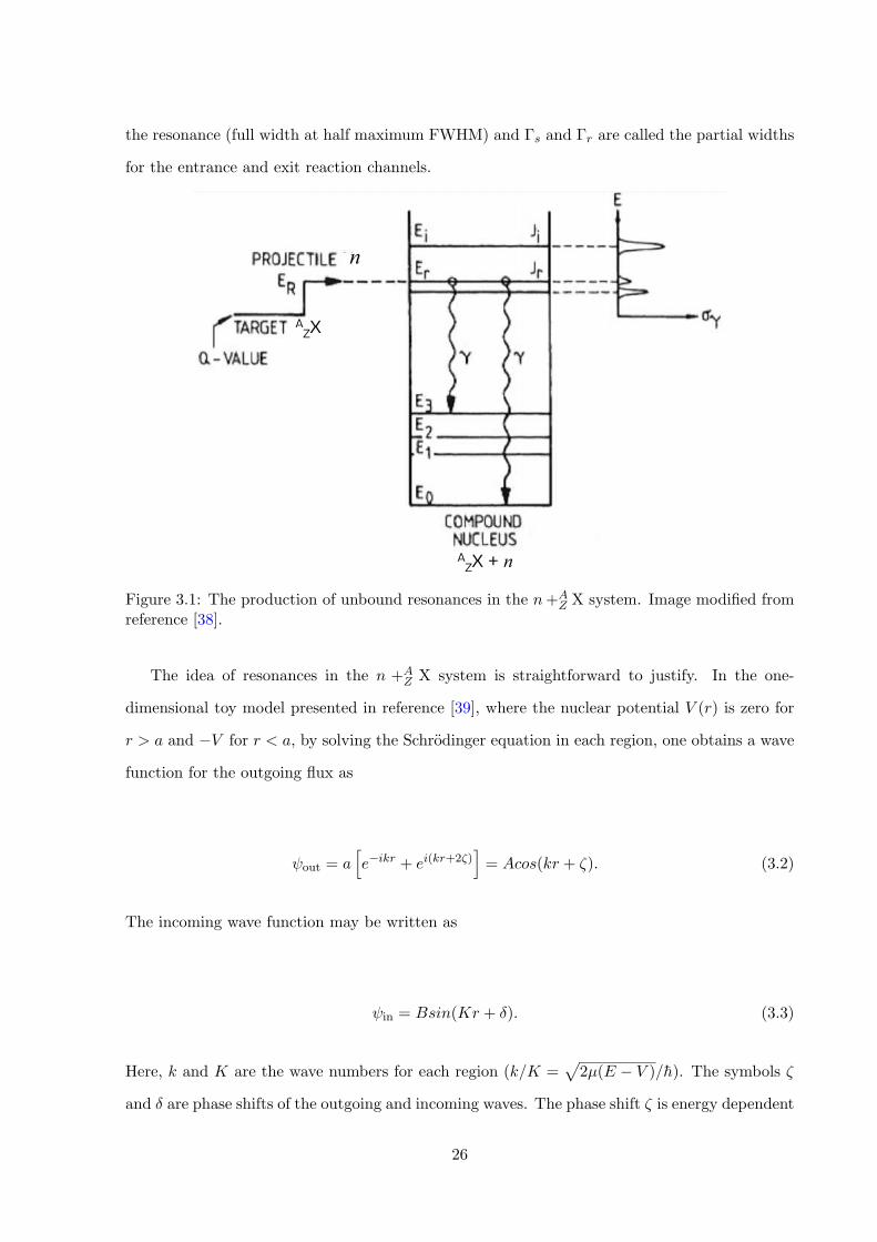
the resonance (full width at half maximum FWHM) and �s and �r are called the partial widths

for the entrance and exit reaction channels.

AZX

n

AZX + n

Figure 3.1: The production of unbound resonances in the n+AZ X system. Image modified from

reference [38].

The idea of resonances in the n +AZ X system is straightforward to justify. In the one-

dimensional toy model presented in reference [39], where the nuclear potential V (r) is zero for

r > a and �V for r < a, by solving the Schrodinger equation in each region, one obtains a wave

function for the outgoing flux as

out = ahe�ikr + ei(kr+2⇣)

i= Acos(kr + ⇣). (3.2)

The incoming wave function may be written as

in = Bsin(Kr + �). (3.3)

Here, k and K are the wave numbers for each region (k/K =p

2µ(E � V )/h). The symbols ⇣

and � are phase shifts of the outgoing and incoming waves. The phase shift ⇣ is energy dependent

26

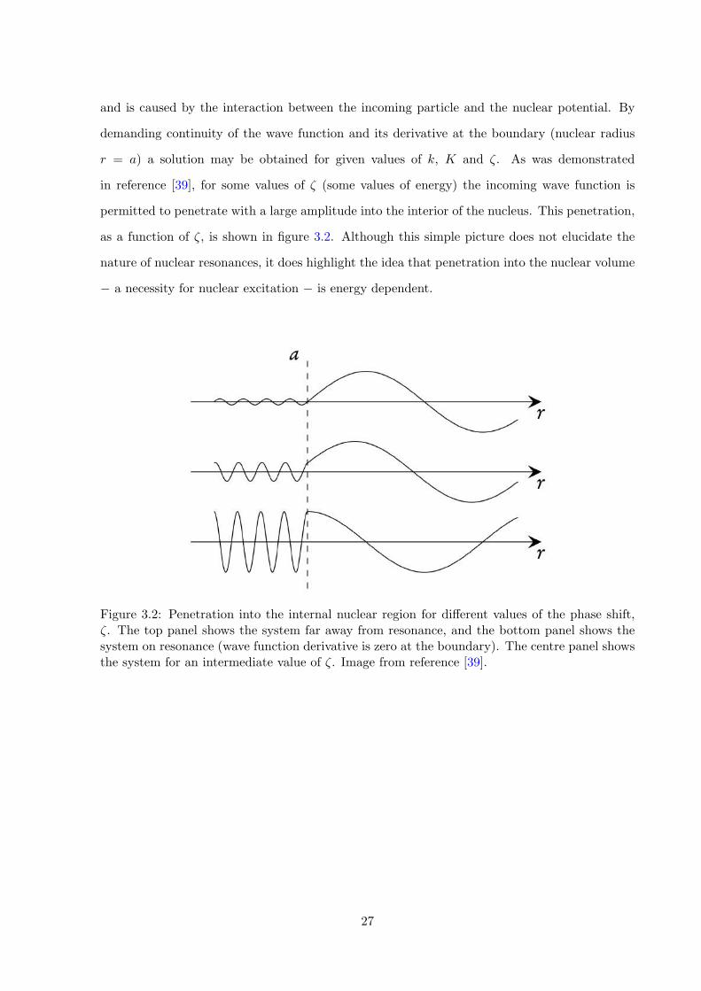
and is caused by the interaction between the incoming particle and the nuclear potential. By

demanding continuity of the wave function and its derivative at the boundary (nuclear radius

r = a) a solution may be obtained for given values of k, K and ⇣. As was demonstrated

in reference [39], for some values of ⇣ (some values of energy) the incoming wave function is

permitted to penetrate with a large amplitude into the interior of the nucleus. This penetration,

as a function of ⇣, is shown in figure 3.2. Although this simple picture does not elucidate the

nature of nuclear resonances, it does highlight the idea that penetration into the nuclear volume

� a necessity for nuclear excitation � is energy dependent.

Figure 3.2: Penetration into the internal nuclear region for di↵erent values of the phase shift,⇣. The top panel shows the system far away from resonance, and the bottom panel shows thesystem on resonance (wave function derivative is zero at the boundary). The centre panel showsthe system for an intermediate value of ⇣. Image from reference [39].

27

3.2 Introduction to R-Matrix theory

A key feature that has not yet been discussed is the repulsive potential barrier from Coulomb

and angular momentum between the two reacting nuclei. The existence of these barriers pro-

duce a classically-forbidden region outside of the nuclear volume, which modifies the coupling

between states in the core and in the continuum. Hence, the simple Breit-Wigner cross section

presented by equation 3.1 does not tell the full story.

In order to interpret nuclear cross sections, R-Matrix theory is required. A detailed review

of this analysis framework can be found in reference [40] and a pedagogical text on the subject

is given by reference [41]. This section aims to provide an introductory overview of the topic

and provides some key results. In R-Matrix theory, the nucleus is treated as a compound sys-

tem, which may be excited or de-excited through various channels. The channels correspond

to di↵erent projectile-target combinations, channel spins, and relative angular momenta. For

example, 16O may be excited, or may decay, through a variety of channels. These include, but

are not limited to, the 12C + 4He channel, the 8Be + 8Be channel, or through excited states

in these nuclei, which may correspond to di↵erent angular momenta. The aim of an R-matrix

analysis is to calculate the reaction cross section, �c0c, given an entrance channel, c’, and an exit

channel, c.

Using this method, the compound nuclear system is separated into two regions: an internal

region where the nuclear force dominates, and an external region, beyond the e↵ects of the

nuclear interaction, where only the Coulomb force comes into play. The point separating these

regions is called the channel radius, and for a pair of particles 1 and 2, it is typically defined as

ac = r0

⇣A

1/31 +A

1/32

⌘. (3.4)

The parameter r0 is around 1.35 fm. Since r0A1/3 is the radius of a nucleus of mass A, equation

3.4 describes the case where the two nuclei in the channel are just ‘touching.’ The internal

nuclear system is modelled as a number of states labelled by i, with energies Ei, total angular

momentum and parity J⇡ii . These states couple to the channel c by a reduced width amplitude �ic.

28

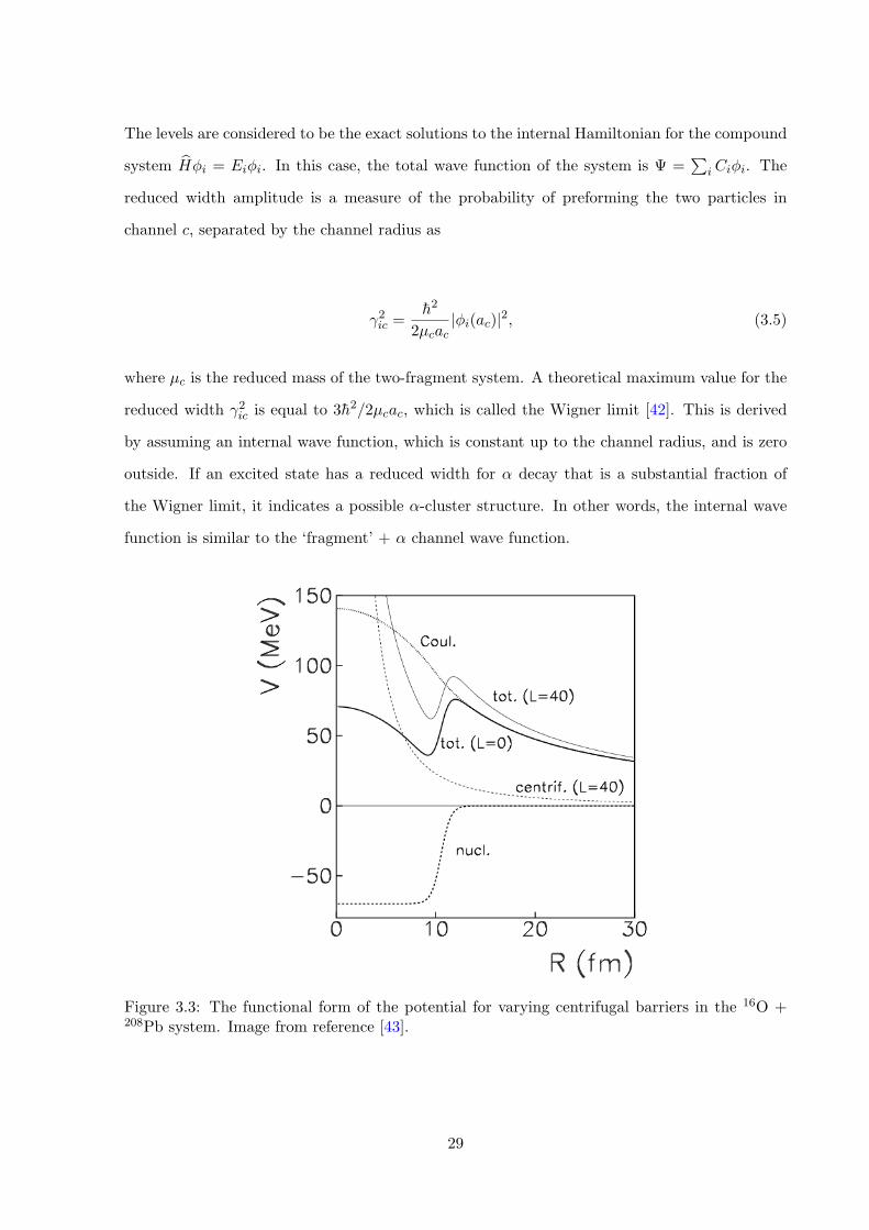
The levels are considered to be the exact solutions to the internal Hamiltonian for the compound

system bH�i = Ei�i. In this case, the total wave function of the system is =P

iCi�i. The

reduced width amplitude is a measure of the probability of preforming the two particles in

channel c, separated by the channel radius as

�2ic =h2

2µcac|�i(ac)|2, (3.5)

where µc is the reduced mass of the two-fragment system. A theoretical maximum value for the

reduced width �2ic is equal to 3h2/2µcac, which is called the Wigner limit [42]. This is derived

by assuming an internal wave function, which is constant up to the channel radius, and is zero

outside. If an excited state has a reduced width for ↵ decay that is a substantial fraction of

the Wigner limit, it indicates a possible ↵-cluster structure. In other words, the internal wave

function is similar to the ‘fragment’ + ↵ channel wave function.

Figure 3.3: The functional form of the potential for varying centrifugal barriers in the 16O +208Pb system. Image from reference [43].

29

The coupling between an internal level and a channel c is not just determined by the internal

properties of the system; the Coulomb and angular momentum barriers suppress the ability of

the nucleus to emit the appropriate pair of particles from the channel radius. The Coulomb and

centrifugal barriers for a two-body system are shown in figure 3.3. The coupling is a↵ected by

the penetrability through the barrier Pc(Ei), meaning that a partial width �ic must be defined

as

�ic = 2Pc(Ei)�2ic, (3.6)

and the total width of a state is given by the sum of all of the partial widths of the open

channels. Using R-Matrix theory, it is possible to derive the reaction cross section. In order

to ignore interference e↵ects between di↵erent states, the following discussion focusses on an

isolated resonance. For a narrow resonance, where the decay penetrability for the channel does

not increase significantly over the total width of the resonance, the simple Breit-Wigner form of

equation 3.12 is obtained

�c0c / �ic0�ic(E � Er)2 + (�i/2)2

. (3.7)

The measured resonance energy di↵ers from the level energy by an amount equal to the level

shift so Er = Ei+�i(Er). This may be calculated from the shift function, Sc(E) [44]. Similarly,

the observed level widths also vary by an amount dictated by the shift function.

�ic(E) = �(Sc(E)�Bc)�2ic (3.8)

�ic(obs.) =�2ic

1 +P

c �2ic

dSdE |Er

. (3.9)

Typically Bc is set to equal Sc(Er) when working with isolated resonances. The shift function

and the penetrability are calculated in terms of regular and irregular Coulomb wave functions

evaluated at the channel radius F`(Kac) and G`(Kac) as

30

S`i(E) = P`i(E)⇥F`(Kac)F

0`(Kac) +G`(Kac)G

0`(Kac)

⇤and (3.10)

P`i(E) =Kac

F`(Kac)2 +G`(Kac)2(3.11)

respectively, where F 0`(Kac) and G0

`(Kac) indicate derivatives of these functions with respect to

Kac (K =p2µcE/h) and ` is the orbital angular momentum of the channel.

The cross section for an isolated broad resonance is parameterised similar to a simple Breit-

Wigner profile but with an energy-dependent resonance energy and width

�c0c / �ic0(E)�ic(E)

(E � Ei ��ic(E))2 + (�i(E)/2)2. (3.12)

Therefore, rather than the symmetric Breit-Wigner line shape, more complicated asymmetric

resonance profiles are expected for broader states. In a very extreme case, the multiplication of

the increasing penetrability factor in the numerator of equation 3.12, via equation 3.6, with the

decreasing Breit-Wigner tail of the resonance may result in the appearance of a ghost state [45,

46]. Both the 0+ Hoyle state in 12C and the 8Be ground state have accompanying ghost states

[47–50].

To derive these results, the R-matrix for an incoming and outgoing channel must be constructed

Rc0c =NX

i=1

�ic�ic0

Eir � E

, (3.13)

which has N resonances at energies E = Eir. As can be seen, the R-matrix is a function of

energy, E, the resonance energies, Eir, and the reduced channel widths, �ic and �ic0 . Another

object called the S-matrix is defined as

S =1�R(S � iP � ac�)

1�R(S + iP � ac�)e2i�, (3.14)

31

where � is called the hard-sphere phase shift given as � = �atan(F/G) and � is a free parameter.

The cross section is calculated from this S-matrix [44].

In reality, an experimentalist can measure an excitation spectrum/ reaction cross section over

many scattering angles and through a variety of di↵erent incoming and outgoing channels. Such

cross sections may include numerous resonances that are populated during the experiment. The

challenge is then to extract the properties of these resonances using an R-matrix fit to the data.

As has been mentioned, the properties of resonances, in particular the reduced channel widths,

can lead to an understanding of the degree of clustering of the nuclear states. One program

that can perform an R-matrix fit is called AZURE2 [51]. During a fit to experimental data, the

resonance energies and reduced widths are varied such that the cross section, calculated from

the S-matrix, best fits the experimental data. This is evaluated through a �2 minimisation

procedure.

32

Chapter 4

Molecular structures in the mirror

nuclei, beryllium-9 and boron-9

Doesmychargeradiuslookbig

inthis..?

np

34

Chapter abstract

Beryllium-9 is thought to be the simplest example of a nuclear molecule. Whereas 8Be is unstable

to ↵ decay, 9Be is not; the extra valence neutron is though to exist in either �- or ⇡-type orbitals

about two ↵-particle cores, increasing the binding energy. In this sense, the neutronic motion is

analogous to electron orbits in atomic molecules. Three rotational bands in 9Be have been iden-

tified in the past, corresponding to the collective rotations of various molecular configurations.

A fourth rotational band, corresponding to the ⇡-antibinding configuration, is predicted but has

not yet been experimentally identified. To investigate the 9Be excitation spectrum, the inelastic

scattering and break-up reaction 9Be(4He,3↵)n was measured using an array of double-sided

silicon strip detectors at beam energies of 22 and 26 MeV. Excited states in 9Be up to 8 MeV

were populated and reconstructed through measurements of the final state reaction products.

Evidence is provided for a state in 9Be at 3.82+0.08�0.09 MeV with a width � = 1240+270

�90 keV. These

parameters are consistent with two recent measurements of a new state in the mirror nucleus,

9B. Analysing the reduced width of the state (8Beg.s. channel), along with that of the proposed

mirror state in 9B, has led to a firm limit on the angular momentum J 7/2 and a tentative

assignment of J⇡ = 1/2� or 3/2�. This leaves the possibility that the newly-measured state is

the hitherto unseen ⇡-antibinding molecular band head.

This work has been published in the following articles. Some figures and text blocks from these

publications are used in the following chapter.

R. Smith, M. Freer, C. Wheldon, N. Curtis, Tz. Kokalova, et al. Disentangling unclear nuclear

breakup channels of beryllium-9 using the three-axis Dalitz plot. Journal of Physics: Conf. Series

863 (2017).

R. Smith, C. Wheldon, M. Freer, N. Curtis, Tz. Kokalova, et al. Evidence for a 3.8 MeV state

in 9Be. Physical Review C 94 (2016).

R. Smith, C. Wheldon, M. Freer, N. Curtis, Tz. Kokalova, et al. Breakup branches of Borromean

beryllium-9. Proceedings of Nuclear Structure and Dynamics 15. Vol. 1681. AIP Publishing,

(2015).

35

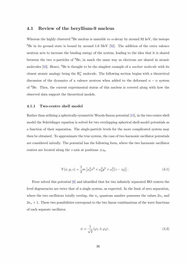
4.1 Review of the beryllium-9 nucleus

Whereas the highly clustered 8Be nucleus is unstable to ↵-decay by around 92 keV, the isotope

9Be in its ground state is bound by around 1.6 MeV [52]. The addition of the extra valence

neutron acts to increase the binding energy of the system, leading to the idea that it is shared

between the two ↵-particles of 8Be, in much the same way as electrons are shared in atomic

molecules [53]. Hence, 9Be is thought to be the simplest example of a nuclear molecule with its

closest atomic analogy being the H+2 molecule. The following section begins with a theoretical

discussion of the dynamics of a valence neutron when added to the deformed ↵ � ↵ system

of 8Be. Then, the current experimental status of this nucleus is covered along with how the

observed data support the theoretical models.

4.1.1 Two-centre shell model

Rather than utilising a spherically-symmetric Woods-Saxon potential [15], in the two-centre shell

model the Schrodinger equation is solved for two overlapping spherical shell-model potentials as

a function of their separation. The single-particle levels for the more complicated system may

then be obtained. To approximate the true system, the case of two harmonic oscillator potentials

are considered initially. The potential has the following form, where the two harmonic oscillator

centres are located along the z-axis at positions ±z0,

V (x, y, z) =1

2m⇥!2xx

2 + !2yy

2 + !2z(z � z0)

⇤. (4.1)

Freer solved this potential [6] and identified that for two infinitely separated HO centres the

level degeneracies are twice that of a single system, as expected. In the limit of zero separation,

where the two oscillators totally overlap, the nz quantum number possesses the values 2nz and

2nz + 1. These two possibilities correspond to the two linear combinations of the wave functions

of each separate oscillator.

=1p2('1 ± '2) . (4.2)

36

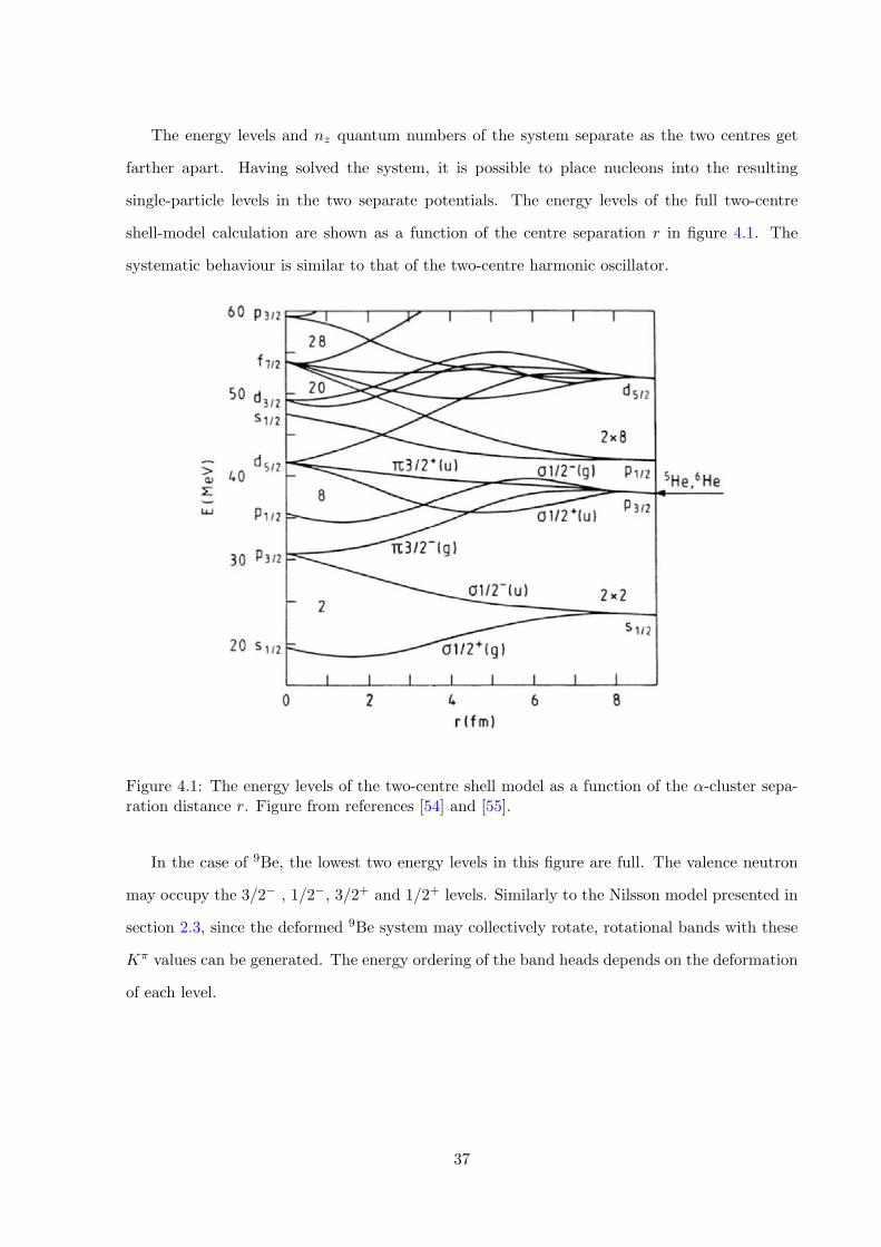
The energy levels and nz quantum numbers of the system separate as the two centres get

farther apart. Having solved the system, it is possible to place nucleons into the resulting

single-particle levels in the two separate potentials. The energy levels of the full two-centre

shell-model calculation are shown as a function of the centre separation r in figure 4.1. The

systematic behaviour is similar to that of the two-centre harmonic oscillator.

Figure 4.1: The energy levels of the two-centre shell model as a function of the ↵-cluster sepa-ration distance r. Figure from references [54] and [55].

In the case of 9Be, the lowest two energy levels in this figure are full. The valence neutron

may occupy the 3/2� , 1/2�, 3/2+ and 1/2+ levels. Similarly to the Nilsson model presented in

section 2.3, since the deformed 9Be system may collectively rotate, rotational bands with these

K⇡ values can be generated. The energy ordering of the band heads depends on the deformation

of each level.

37

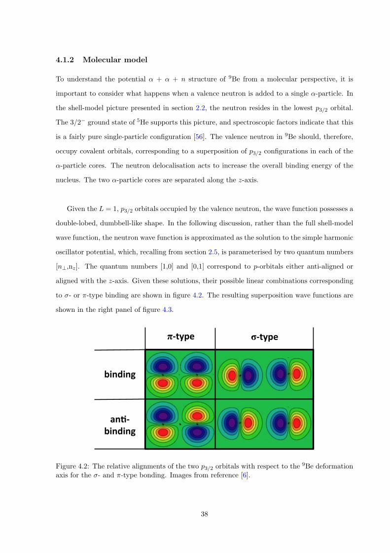
4.1.2 Molecular model

To understand the potential ↵ + ↵ + n structure of 9Be from a molecular perspective, it is

important to consider what happens when a valence neutron is added to a single ↵-particle. In

the shell-model picture presented in section 2.2, the neutron resides in the lowest p3/2 orbital.

The 3/2� ground state of 5He supports this picture, and spectroscopic factors indicate that this

is a fairly pure single-particle configuration [56]. The valence neutron in 9Be should, therefore,

occupy covalent orbitals, corresponding to a superposition of p3/2 configurations in each of the

↵-particle cores. The neutron delocalisation acts to increase the overall binding energy of the

nucleus. The two ↵-particle cores are separated along the z-axis.

Given the L = 1, p3/2 orbitals occupied by the valence neutron, the wave function possesses a

double-lobed, dumbbell-like shape. In the following discussion, rather than the full shell-model

wave function, the neutron wave function is approximated as the solution to the simple harmonic

oscillator potential, which, recalling from section 2.5, is parameterised by two quantum numbers

[n?,nz]. The quantum numbers [1,0] and [0,1] correspond to p-orbitals either anti-aligned or

aligned with the z-axis. Given these solutions, their possible linear combinations corresponding

to �- or ⇡-type binding are shown in figure 4.2. The resulting superposition wave functions are

shown in the right panel of figure 4.3.

π-type σ-type

binding

an--binding

Figure 4.2: The relative alignments of the two p3/2 orbitals with respect to the 9Be deformationaxis for the �- and ⇡-type bonding. Images from reference [6].

38

[001]±[001] [100]±[100]

Figure 4.3: Left: energy levels of the two centre shell model. Right: the �- and ⇡-type molec-ular orbital wave functions associated with the valence neutron in 9Be. These correspond tosuperpositions of [1,0,0] and [0,0,1] ([nx, ny, nz]) harmonic oscillator wave functions. Imagesfrom references [55] and [6].

The two-centre shell model and molecular-orbit model are complementary descriptions of

the 9Be system. For example, the 3/2� ⇡-binding orbital in the right of figure 4.3 is the most

compact arrangement so has a smaller deformation and moment of inertia. The 1/2+ �-binding

configuration on the other hand has a larger moment of inertia, and the neutron density in the

centre acts to separate out the ↵-particle cores. These correspond to the ground state and first

excited state of 9Be. In the two-centre shell-model diagram on the left of figure 4.3, the only way

that this energy level ordering may occur is if the 1/2+ level has a much larger ↵�↵ separation

r, which is entirely consistent with the molecular picture. The same systematics are observed

in the experimental data (section 4.1.4).

The calculations of references [57, 58], using the generator coordinate method, calculated

energy curves for the states in 9Be as a function of the ↵ � ↵ separation. The levels reach

their respective minima at di↵erent separations, supporting the picture presented in figure 4.3.

In this model there was found to be close to 100% overlap between the obtained ground state

wave function and that of the pure K = 3/2� ⇡-binding configuration. For the 1/2+ level, a

39

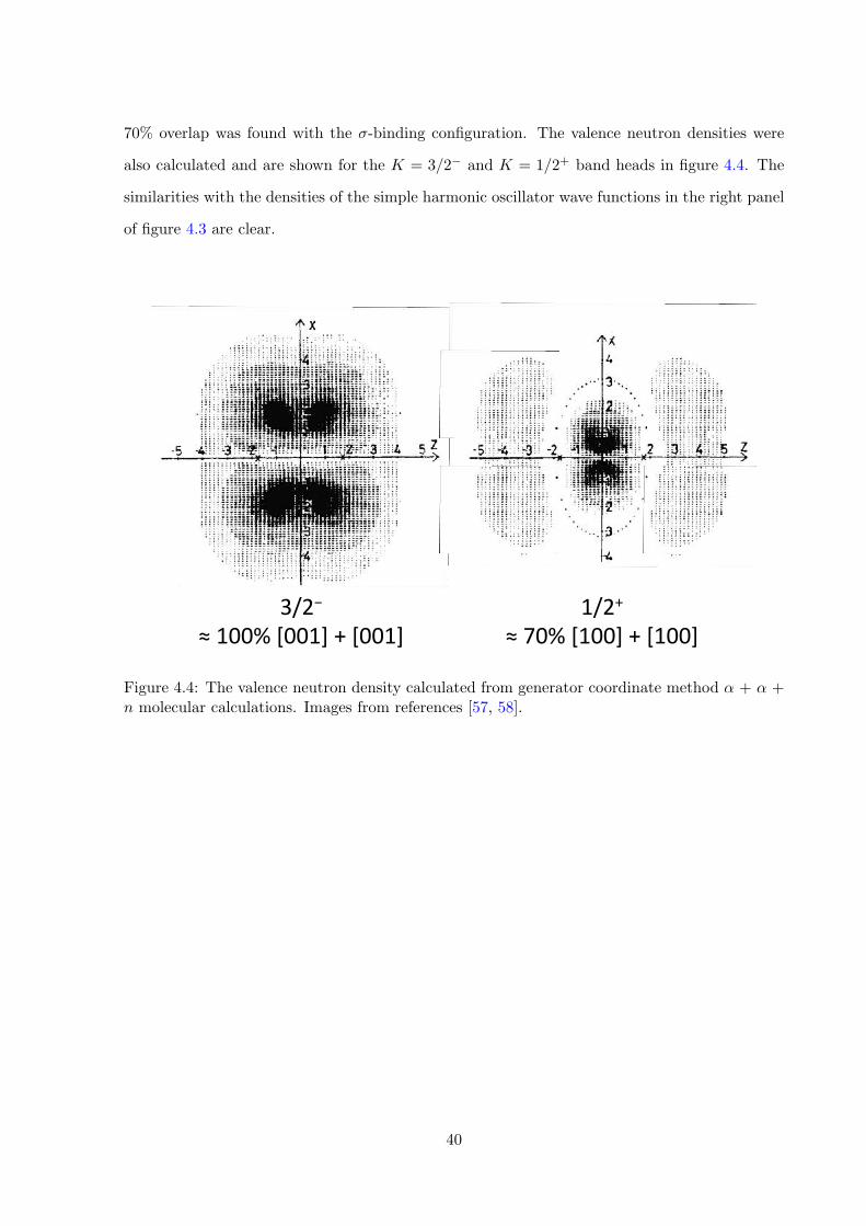
70% overlap was found with the �-binding configuration. The valence neutron densities were

also calculated and are shown for the K = 3/2� and K = 1/2+ band heads in figure 4.4. The

similarities with the densities of the simple harmonic oscillator wave functions in the right panel

of figure 4.3 are clear.

3/2−≈100%[001]+[001]

1/2+≈70%[100]+[100]

Figure 4.4: The valence neutron density calculated from generator coordinate method ↵ + ↵ +n molecular calculations. Images from references [57, 58].

40

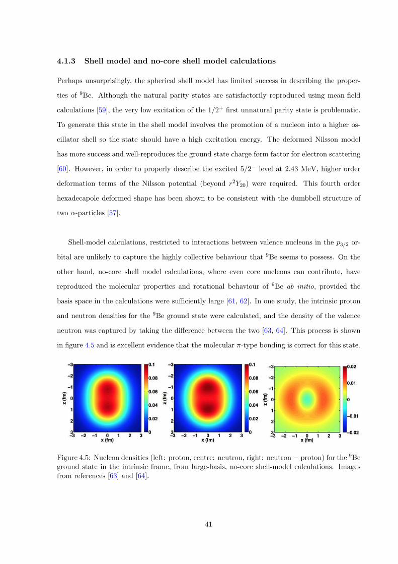
4.1.3 Shell model and no-core shell model calculations

Perhaps unsurprisingly, the spherical shell model has limited success in describing the proper-

ties of 9Be. Although the natural parity states are satisfactorily reproduced using mean-field

calculations [59], the very low excitation of the 1/2+ first unnatural parity state is problematic.

To generate this state in the shell model involves the promotion of a nucleon into a higher os-

cillator shell so the state should have a high excitation energy. The deformed Nilsson model

has more success and well-reproduces the ground state charge form factor for electron scattering

[60]. However, in order to properly describe the excited 5/2� level at 2.43 MeV, higher order

deformation terms of the Nilsson potential (beyond r2Y20) were required. This fourth order

hexadecapole deformed shape has been shown to be consistent with the dumbbell structure of

two ↵-particles [57].

Shell-model calculations, restricted to interactions between valence nucleons in the p3/2 or-

bital are unlikely to capture the highly collective behaviour that 9Be seems to possess. On the

other hand, no-core shell model calculations, where even core nucleons can contribute, have

reproduced the molecular properties and rotational behaviour of 9Be ab initio, provided the

basis space in the calculations were su�ciently large [61, 62]. In one study, the intrinsic proton

and neutron densities for the 9Be ground state were calculated, and the density of the valence

neutron was captured by taking the di↵erence between the two [63, 64]. This process is shown

in figure 4.5 and is excellent evidence that the molecular ⇡-type bonding is correct for this state.

Figure 4.5: Nucleon densities (left: proton, centre: neutron, right: neutron � proton) for the 9Beground state in the intrinsic frame, from large-basis, no-core shell-model calculations. Imagesfrom references [63] and [64].

41

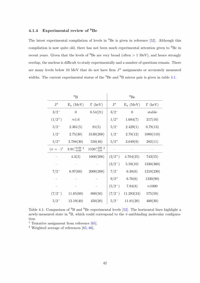
4.1.4 Experimental review of 9Be

The latest experimental compilation of levels in 9Be is given in reference [52]. Although this

compilation is now quite old, there has not been much experimental attention given to 9Be in

recent years. Given that the levels of 9Be are very broad (often > 1 MeV), and hence strongly

overlap, the nucleus is di�cult to study experimentally and a number of questions remain. There

are many levels below 10 MeV that do not have firm J⇡ assignments or accurately measured

widths. The current experimental status of the 9Be and 9B mirror pair is given in table 4.1.

9B 9Be

J⇡ Ex (MeV) � (keV) J⇡ Ex (MeV) � (keV)

3/2� 0 0.54(21) 3/2� 0 stable

(1/2+) ⇡1.6 – 1/2+ 1.684(7) 217(10)

5/2� 2.361(5) 81(5) 5/2� 2.429(1) 0.78(13)

1/2� 2.75(30) 3130(200) 1/2� 2.78(12) 1080(110)

5/2+ 2.788(30) 550(40) 5/2+ 3.049(9) 282(11)

(⇡ = –)1 3.91+0.09�0.09

2 1520+230�210

2 – – –

– 4.3(2) 1600(200) (3/2+) 4.704(25) 743(55)

– – – (3/2�) 5.59(10) 1330(360)

7/2� 6.97(60) 2000(200) 7/2� 6.38(6) 1210(230)

– – – 9/2+ 6.76(6) 1330(90)

– – – (5/2�) 7.94(8) ⇡1000

(7/2�) 11.65(60) 800(50) (7/2�) 11.283(24) 575(50)

5/2� 12.19(40) 450(20) 5/2� 11.81(20) 400(30)

Table 4.1: Comparison of 9B and 9Be experimental levels [52]. The horizontal lines highlight anewly-measured state in 9B, which could correspond to the ⇡-antibinding molecular configura-tion.1 Tentative assignment from reference [65].2 Weighted average of references [65, 66].

42

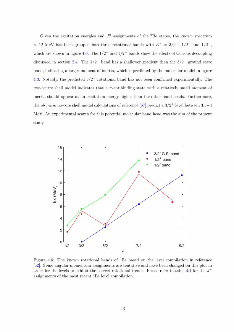
Given the excitation energies and J⇡ assignments of the 9Be states, the known spectrum

< 12 MeV has been grouped into three rotational bands with K⇡ = 3/2�, 1/2+ and 1/2�,

which are shown in figure 4.6. The 1/2+ and 1/2� bands show the e↵ects of Coriolis decoupling

discussed in section 2.4. The 1/2+ band has a shallower gradient than the 3/2� ground state

band, indicating a larger moment of inertia, which is predicted by the molecular model in figure

4.3. Notably, the predicted 3/2+ rotational band has not been confirmed experimentally. The

two-centre shell model indicates that a ⇡-antibinding state with a relatively small moment of

inertia should appear at an excitation energy higher than the other band heads. Furthermore,

the ab initio no-core shell model calculations of reference [67] predict a 3/2+ level between 3.5�4

MeV. An experimental search for this potential molecular band head was the aim of the present

study.

0.5 1.5 2.5 3.5 4.5J

0

2

4

6

8

10

12

14

16

Ex (M

eV)

3/2- G.S. band 1/2+ band 1/2- band

1/2 3/2 5/2

3/2

7/2 9/2

Figure 4.6: The known rotational bands of 9Be based on the level compilation in reference[52]. Some angular momentum assignments are tentative and have been changed on this plot inorder for the levels to exhibit the correct rotational trends. Please refer to table 4.1 for the J⇡

assignments of the most recent 9Be level compilation.

43

4.1.5 Mirror nuclei

Much can be learned about a nucleus by examining its mirror partner. Mirror pairs of nuclei

are the same, except the number of protons and neutrons are switched. States of the same

isospin, T , in a set of nuclei with the same mass number, A, but with di↵ering numbers of

protons and neutrons, Z and N , are more generally named isobaric analogue states (IAS). It

is known that the nuclear two-body interaction is approximately charge-independent, meaning

that the nuclear potential between two neutrons, Vnn, is the same as that between two protons,

Vpp [68]. Due to this property of the nuclear force, the many-body Hamiltonians for two mirror

systems are the same, except for the di↵erent Coulomb interactions. The two nuclei should

exhibit similar properties, aside from the fact that their levels will be shifted by a calculable

amount due to the di↵erence in the Coulomb energy [69, 70]. For cross section measurements

in nuclear astrophysics, the properties of mirror nuclei are important. The symmetry between

mirror nuclei sometimes means that astrophysically relevant proton capture reaction rates can

be inferred from information obtained from transfer reactions with stable beams [71].

When considering Coulomb energy di↵erences between mirror analogue states, it is useful

to normalise the energies of excited states to those of the corresponding ground states. The

majority of the Coulomb energy di↵erence, which arises due to the di↵erence in bulk Coulomb

energy for the whole nucleus, will then cancel out. Therefore, the important considerations are

how the Coulomb energy varies as a function of excitation energy and angular momentum for

mirror analogue states. As illustrated by figure 4.7, the analogue levels in the 9Be/9B mirror

pair show similar excitation energy-spin systematics/rotational bands. Only states with definite

angular momentum and parity assignments can be confidently grouped in this way. Lines joining

states with tentative J⇡ assignments are speculative, since the energy shift between such mirror

analogue levels is non-trivial to calculate. It is therefore not guaranteed that the energy ordering

is consistent between a pair of mirror nuclei. As previously mentioned, the energy di↵erences

between IAS are due to isospin non-conserving forces, such as the Coulomb interaction. In

these systems, the evolution of the Coulomb energy di↵erence with angular momentum is quite

sensitive to di↵erences in nuclear structure [72, 73].

44

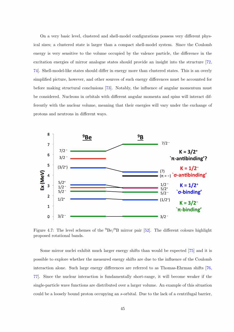
On a very basic level, clustered and shell-model configurations possess very di↵erent phys-

ical sizes; a clustered state is larger than a compact shell-model system. Since the Coulomb

energy is very sensitive to the volume occupied by the valence particle, the di↵erence in the

excitation energies of mirror analogue states should provide an insight into the structure [72,

74]. Shell-model-like states should di↵er in energy more than clustered states. This is an overly

simplified picture, however, and other sources of such energy di↵erences must be accounted for

before making structural conclusions [73]. Notably, the influence of angular momentum must

be considered. Nucleons in orbitals with di↵erent angular momenta and spins will interact dif-

ferently with the nuclear volume, meaning that their energies will vary under the exchange of

protons and neutrons in di↵erent ways.

K=3/2−`π-binding’

K=1/2+`σ-binding’

K=1/2−`σ-an5binding’

3/2–

5/2–

1/2+

5/2+

(3/2+)

1/2–

3/2–

3/2–

5/2–

(1/2+)

5/2+

(?)

1/2–

7/2–7/2–

(π=−)

9Be 9B

K=3/2+`π-an5binding’?

Figure 4.7: The level schemes of the 9Be/9B mirror pair [52]. The di↵erent colours highlightproposed rotational bands.

Some mirror nuclei exhibit much larger energy shifts than would be expected [75] and it is

possible to explore whether the measured energy shifts are due to the influence of the Coulomb

interaction alone. Such large energy di↵erences are referred to as Thomas-Ehrman shifts [76,

77]. Since the nuclear interaction is fundamentally short-range, it will become weaker if the

single-particle wave functions are distributed over a larger volume. An example of this situation

could be a loosely bound proton occupying an s-orbital. Due to the lack of a centrifugal barrier,

45

this orbital can have very large radius. The resulting di↵erence in the single-particle energy

leads to a di↵erence in the wave functions between protons and neutrons. This a↵ects the ma-

trix elements of the residual nuclear interaction, even though the original nucleon-nucleon force

is charge-symmetric.

The channel widths of mirror analogue states can provide an insight into their angular mo-

mentum and parity. In the 9B nucleus, a broad level close to 4 MeV was recently measured

[65, 66]. Aside from one other state, the levels in this energy region have firm J⇡ assignments,

meaning that this new level could correspond to the missing ⇡-antibinding molecular configu-

ration band head. By measuring the properties of a mirror analogue state in 9Be, it could be

possible to infer its angular momentum and parity. Due to the similar 9Be/9B wave functions,

their couplings to the respective 8Be + n and 8Be + p decay channels, defined by the reduced

channel width (section 3.2), should be the same [78]. Therefore, their measured channel widths

(i.e. the partial widths of the mirror states) should di↵er only due to the extra Coulomb barrier

penetrability required for the proton decay. The aim of this experiment was to measure the

properties of the hitherto-unmeasured mirror analogue state in 9Be and to use its properties in

conjunction with that of the 9B state to analyse the nuclear structure.

46

4.2 Experimental details and apparatus

The experimental measurements were performed using the 10 MV FN Tandem Van de Graa↵

accelerator housed at the Nuclear Science Laboratory at the University of Notre Dame. A

4He beam was incident on a thick 1000 µg cm�2 9Be target foil and data were acquired for a

cumulative time of around 30 hours at an average beam current of 2 enA. Two beam energies

of 22 and 26 MeV were used to acquire the data presented in this chapter. The experimental

work was a collaborative e↵ort between researchers from the Universities of Birmingham, Notre

Dame, Wisconsin and the Weizmann Institute.

4.2.1 Notre Dame tandem Van De Graa↵ accelerator

This section describes the principles of operation of the FN Tandem Van de Graa↵ accelerator

[79]. Often the subject of high school demonstrations, a Van de Graa↵ generator is a simple

machine which produces a very high electric potential by collecting electrostatic charge from a

source and gradually transferring it to a large, isolated metal anode through a rotating conveyor

belt. This principle is illustrated schematically in figure 4.8a.

Collecting comb

Metal terminal

Conveyor belt

Voltage Supply

Charged comb

Voltage Supply

Beam pipe at vacuum

Internal belt

Stripper foil

Negative ions

Positive ions

a) b)

Collecting comb

Metal terminal

Conveyor belt

Voltage Supply

Charged comb

Voltage Supply

Beam pipe at vacuum

Internal belt

Stripper foil

Negative ions

Positive ions

a) b)

Figure 4.8: a) Expanded view of a generic Van de Graa↵ generator with the main componentslabelled. b) Schematic diagram illustrating the ‘tandem’ acceleration principle and how ions areaccelerated practically using a Van de Graa↵ generator. Image in a) from reference [80].

47

The Van de Graa↵ generator principle was developed as a means to accelerate ions as early

as the 1930’s. Negative ions external to the Van de Graa↵ generator move in the strong 1/r2

electric field produced by the device which accelerates them towards the positively charged an-

ode. A schematic diagram illustrating the tandem Van de Graa↵ acceleration principle is shown

in figure 4.8b. As with a standard generator, the heart of the accelerator consists of a metal

electrode called the ‘terminal.’ A very large positive charge is applied to this terminal via a high

voltage supply and charge-transferring belt.

Without modification, any negative particle accelerated towards the terminal will collide

into it, limiting the usefulness of the device. To overcome this, an evacuated beam pipe made

from insulating glass cylinders passes through the terminal sphere, through the zero electric

field region inside, and then out of the other side where the beam can be extracted to perform

experiments. However, since the ion is negatively charged as it emerges from the other side of

the terminal, it immediately experiences a restoring force back towards the centre of the system.

Left to its own devices, the negative ion would oscillate about the centre of the terminal and

could never be extracted. To overcome this issue, the negative ions pass through a thin (3 µg

cm�2) carbon ‘stripper’ foil in the centre of the accelerator. This ionises the beam and leaves

it in a variety of positive charge states. The name ‘tandem’ accelerator owes itself to the fact

that the now-positive beam is accelerated a second time away from the electrode, towards the

experimental chamber and target.

For the system described so far, each acceleration stage is non-linear and varies as 1/r2

due to the geometry of the electric field. This is problematic for a number of reasons. Firstly,

the weak field at large distances from the terminal means that the negative ions propagate

notable distances at low velocities, meaning that their path through the system is susceptible

to deflections from stray electric fields. Secondly, the high electric field close to the terminal

can cause uncontrollable electric discharges. The issue of non-linearity is solved by constructing

the vacuum tube in segments, consisting of glass cylinders glued to metal electrodes. Equal

value resistors are connected between these electrodes which creates a potential divider circuit.

The voltage di↵erence across each gap is therefore uniform, leading to a uniform acceleration.

This system is shown schematically in figure 4.9a and as a photograph in figure 4.9b. As shown

48

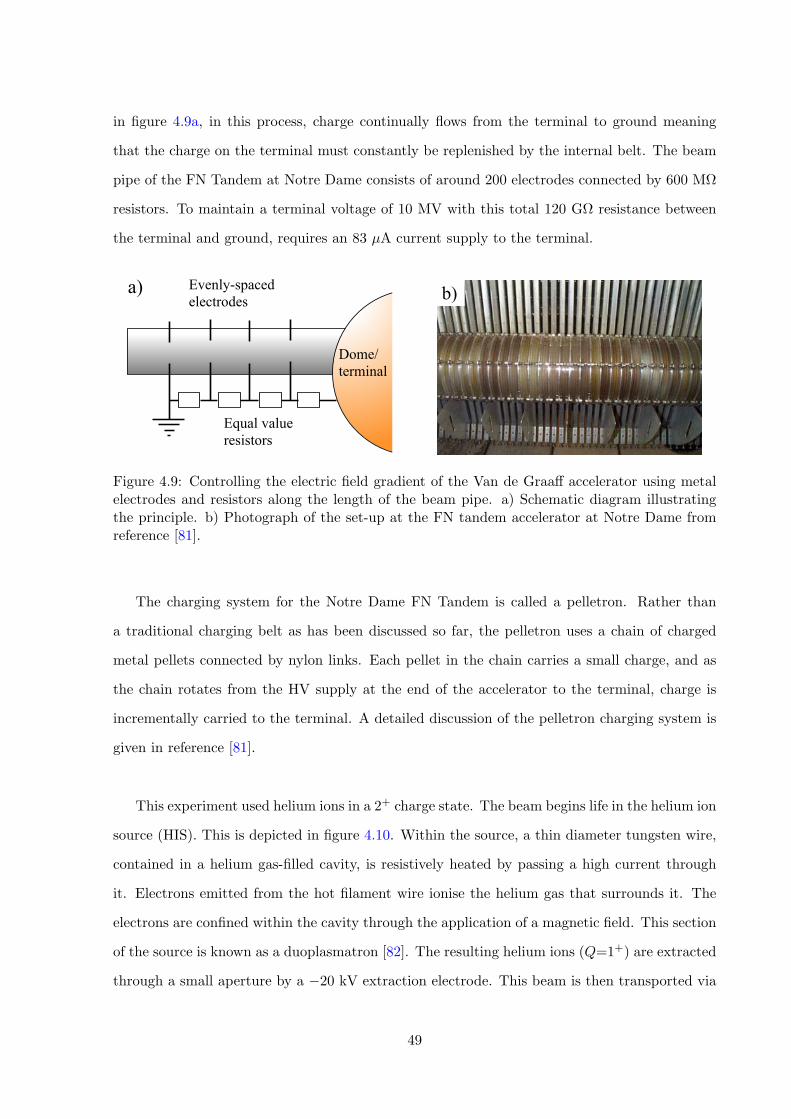
in figure 4.9a, in this process, charge continually flows from the terminal to ground meaning

that the charge on the terminal must constantly be replenished by the internal belt. The beam

pipe of the FN Tandem at Notre Dame consists of around 200 electrodes connected by 600 M⌦

resistors. To maintain a terminal voltage of 10 MV with this total 120 G⌦ resistance between

the terminal and ground, requires an 83 µA current supply to the terminal.

a) b) Evenly-spaced electrodes

Dome/ terminal

Equal value resistors

a) b) Evenly-spaced electrodes

Dome/ terminal

Equal value resistors

Figure 4.9: Controlling the electric field gradient of the Van de Graa↵ accelerator using metalelectrodes and resistors along the length of the beam pipe. a) Schematic diagram illustratingthe principle. b) Photograph of the set-up at the FN tandem accelerator at Notre Dame fromreference [81].

The charging system for the Notre Dame FN Tandem is called a pelletron. Rather than

a traditional charging belt as has been discussed so far, the pelletron uses a chain of charged

metal pellets connected by nylon links. Each pellet in the chain carries a small charge, and as

the chain rotates from the HV supply at the end of the accelerator to the terminal, charge is

incrementally carried to the terminal. A detailed discussion of the pelletron charging system is

given in reference [81].

This experiment used helium ions in a 2+ charge state. The beam begins life in the helium ion

source (HIS). This is depicted in figure 4.10. Within the source, a thin diameter tungsten wire,

contained in a helium gas-filled cavity, is resistively heated by passing a high current through

it. Electrons emitted from the hot filament wire ionise the helium gas that surrounds it. The

electrons are confined within the cavity through the application of a magnetic field. This section

of the source is known as a duoplasmatron [82]. The resulting helium ions (Q=1+) are extracted

through a small aperture by a �20 kV extraction electrode. This beam is then transported via

49

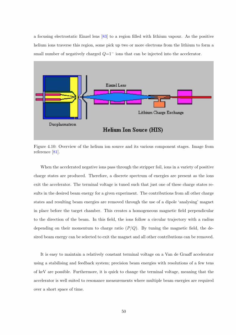
a focusing electrostatic Einzel lens [83] to a region filled with lithium vapour. As the positive

helium ions traverse this region, some pick up two or more electrons from the lithium to form a

small number of negatively charged Q=1� ions that can be injected into the accelerator.

Figure 4.10: Overview of the helium ion source and its various component stages. Image fromreference [81].

When the accelerated negative ions pass through the stripper foil, ions in a variety of positive

charge states are produced. Therefore, a discrete spectrum of energies are present as the ions

exit the accelerator. The terminal voltage is tuned such that just one of these charge states re-

sults in the desired beam energy for a given experiment. The contributions from all other charge

states and resulting beam energies are removed through the use of a dipole ‘analysing’ magnet

in place before the target chamber. This creates a homogeneous magnetic field perpendicular

to the direction of the beam. In this field, the ions follow a circular trajectory with a radius

depending on their momentum to charge ratio (P/Q). By tuning the magnetic field, the de-

sired beam energy can be selected to exit the magnet and all other contributions can be removed.

It is easy to maintain a relatively constant terminal voltage on a Van de Graa↵ accelerator

using a stabilising and feedback system; precision beam energies with resolutions of a few tens

of keV are possible. Furthermore, it is quick to change the terminal voltage, meaning that the

accelerator is well suited to resonance measurements where multiple beam energies are required

over a short space of time.

50

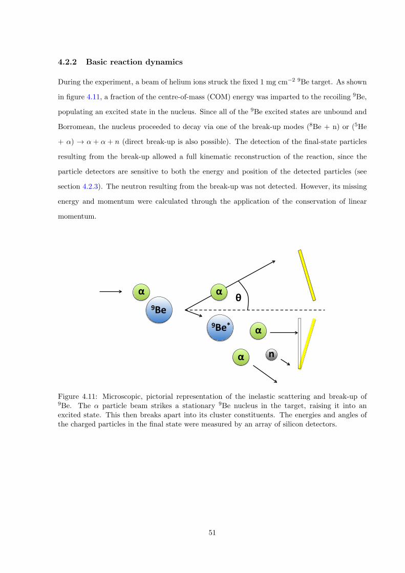
4.2.2 Basic reaction dynamics

During the experiment, a beam of helium ions struck the fixed 1 mg cm�2 9Be target. As shown

in figure 4.11, a fraction of the centre-of-mass (COM) energy was imparted to the recoiling 9Be,

populating an excited state in the nucleus. Since all of the 9Be excited states are unbound and

Borromean, the nucleus proceeded to decay via one of the break-up modes (8Be + n) or (5He

+ ↵) ! ↵ + ↵ + n (direct break-up is also possible). The detection of the final-state particles

resulting from the break-up allowed a full kinematic reconstruction of the reaction, since the

particle detectors are sensitive to both the energy and position of the detected particles (see

section 4.2.3). The neutron resulting from the break-up was not detected. However, its missing

energy and momentum were calculated through the application of the conservation of linear

momentum.

9Be$

9Be*$

α$ α$

α$

α$

n$

θ$

Figure 4.11: Microscopic, pictorial representation of the inelastic scattering and break-up of9Be. The ↵ particle beam strikes a stationary 9Be nucleus in the target, raising it into anexcited state. This then breaks apart into its cluster constituents. The energies and angles ofthe charged particles in the final state were measured by an array of silicon detectors.

51

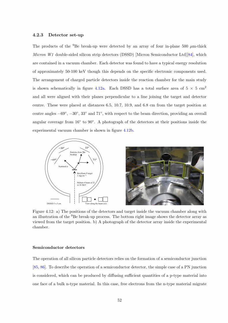
4.2.3 Detector set-up

The products of the 9Be break-up were detected by an array of four in-plane 500 µm-thick

Micron W1 double-sided silicon strip detectors (DSSD) [Micron Semiconductor Ltd][84], which

are contained in a vacuum chamber. Each detector was found to have a typical energy resolution

of approximately 50-100 keV though this depends on the specific electronic components used.

The arrangement of charged particle detectors inside the reaction chamber for the main study

is shown schematically in figure 4.12a. Each DSSD has a total surface area of 5 ⇥ 5 cm2

and all were aligned with their planes perpendicular to a line joining the target and detector

centre. These were placed at distances 6.5, 10.7, 10.9, and 6.8 cm from the target position at

centre angles �69�, �30�, 33� and 71�, with respect to the beam direction, providing an overall

angular coverage from 16� to 90�. A photograph of the detectors at their positions inside the

experimental vacuum chamber is shown in figure 4.12b.

−69!!!!−30!!!!33!!!!71!!!!!

Helium-4 beam at 22 or 26 MeV

View along the beam axis

−69! !!!!

−30! !!!! 33! !!!!

71! !!!!

Beryllium-9 target 1!mg!cm!!

Scattered !

Particles from Be!!

breakup

DSSSD 5 x 5 cm

Figure 4.12: a) The positions of the detectors and target inside the vacuum chamber along withan illustration of the 9Be break-up process. The bottom right image shows the detector array asviewed from the target position. b) A photograph of the detector array inside the experimentalchamber.

Semiconductor detectors

The operation of all silicon particle detectors relies on the formation of a semiconductor junction

[85, 86]. To describe the operation of a semiconductor detector, the simple case of a PN junction

is considered, which can be produced by di↵using su�cient quantities of a p-type material into

one face of a bulk n-type material. In this case, free electrons from the n-type material migrate

52

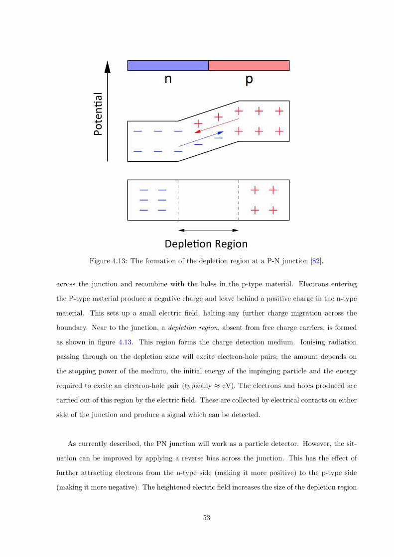
!!!Deple&on!Region!!

Poten&

al!

Figure 4.13: The formation of the depletion region at a P-N junction [82].

across the junction and recombine with the holes in the p-type material. Electrons entering

the P-type material produce a negative charge and leave behind a positive charge in the n-type

material. This sets up a small electric field, halting any further charge migration across the

boundary. Near to the junction, a depletion region, absent from free charge carriers, is formed

as shown in figure 4.13. This region forms the charge detection medium. Ionising radiation

passing through on the depletion zone will excite electron-hole pairs; the amount depends on

the stopping power of the medium, the initial energy of the impinging particle and the energy

required to excite an electron-hole pair (typically ⇡ eV). The electrons and holes produced are

carried out of this region by the electric field. These are collected by electrical contacts on either

side of the junction and produce a signal which can be detected.

As currently described, the PN junction will work as a particle detector. However, the sit-

uation can be improved by applying a reverse bias across the junction. This has the e↵ect of

further attracting electrons from the n-type side (making it more positive) to the p-type side

(making it more negative). The heightened electric field increases the size of the depletion region

53

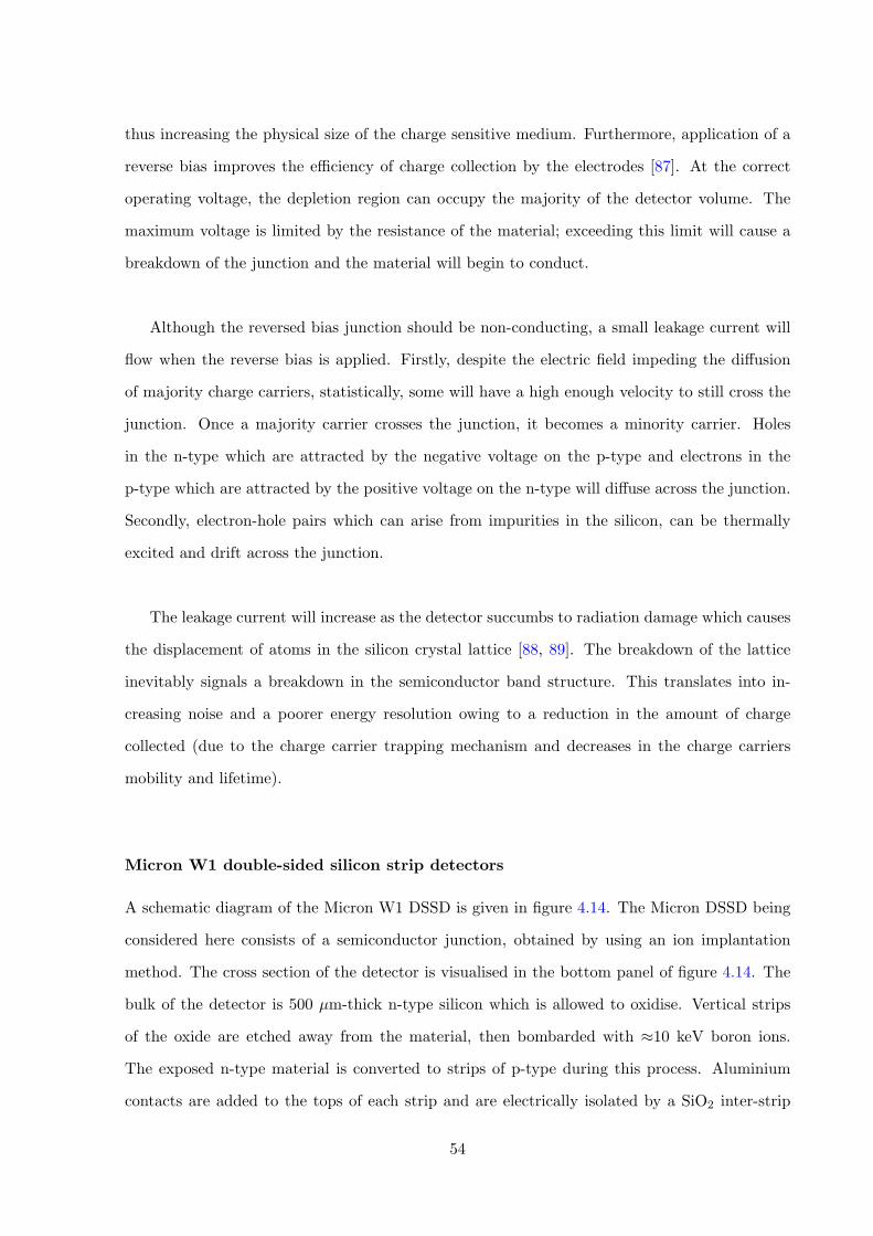
thus increasing the physical size of the charge sensitive medium. Furthermore, application of a

reverse bias improves the e�ciency of charge collection by the electrodes [87]. At the correct

operating voltage, the depletion region can occupy the majority of the detector volume. The

maximum voltage is limited by the resistance of the material; exceeding this limit will cause a

breakdown of the junction and the material will begin to conduct.

Although the reversed bias junction should be non-conducting, a small leakage current will

flow when the reverse bias is applied. Firstly, despite the electric field impeding the di↵usion

of majority charge carriers, statistically, some will have a high enough velocity to still cross the

junction. Once a majority carrier crosses the junction, it becomes a minority carrier. Holes

in the n-type which are attracted by the negative voltage on the p-type and electrons in the

p-type which are attracted by the positive voltage on the n-type will di↵use across the junction.

Secondly, electron-hole pairs which can arise from impurities in the silicon, can be thermally

excited and drift across the junction.

The leakage current will increase as the detector succumbs to radiation damage which causes

the displacement of atoms in the silicon crystal lattice [88, 89]. The breakdown of the lattice

inevitably signals a breakdown in the semiconductor band structure. This translates into in-

creasing noise and a poorer energy resolution owing to a reduction in the amount of charge

collected (due to the charge carrier trapping mechanism and decreases in the charge carriers

mobility and lifetime).

Micron W1 double-sided silicon strip detectors

A schematic diagram of the Micron W1 DSSD is given in figure 4.14. The Micron DSSD being

considered here consists of a semiconductor junction, obtained by using an ion implantation

method. The cross section of the detector is visualised in the bottom panel of figure 4.14. The

bulk of the detector is 500 µm-thick n-type silicon which is allowed to oxidise. Vertical strips

of the oxide are etched away from the material, then bombarded with ⇡10 keV boron ions.

The exposed n-type material is converted to strips of p-type during this process. Aluminium

contacts are added to the tops of each strip and are electrically isolated by a SiO2 inter-strip

54

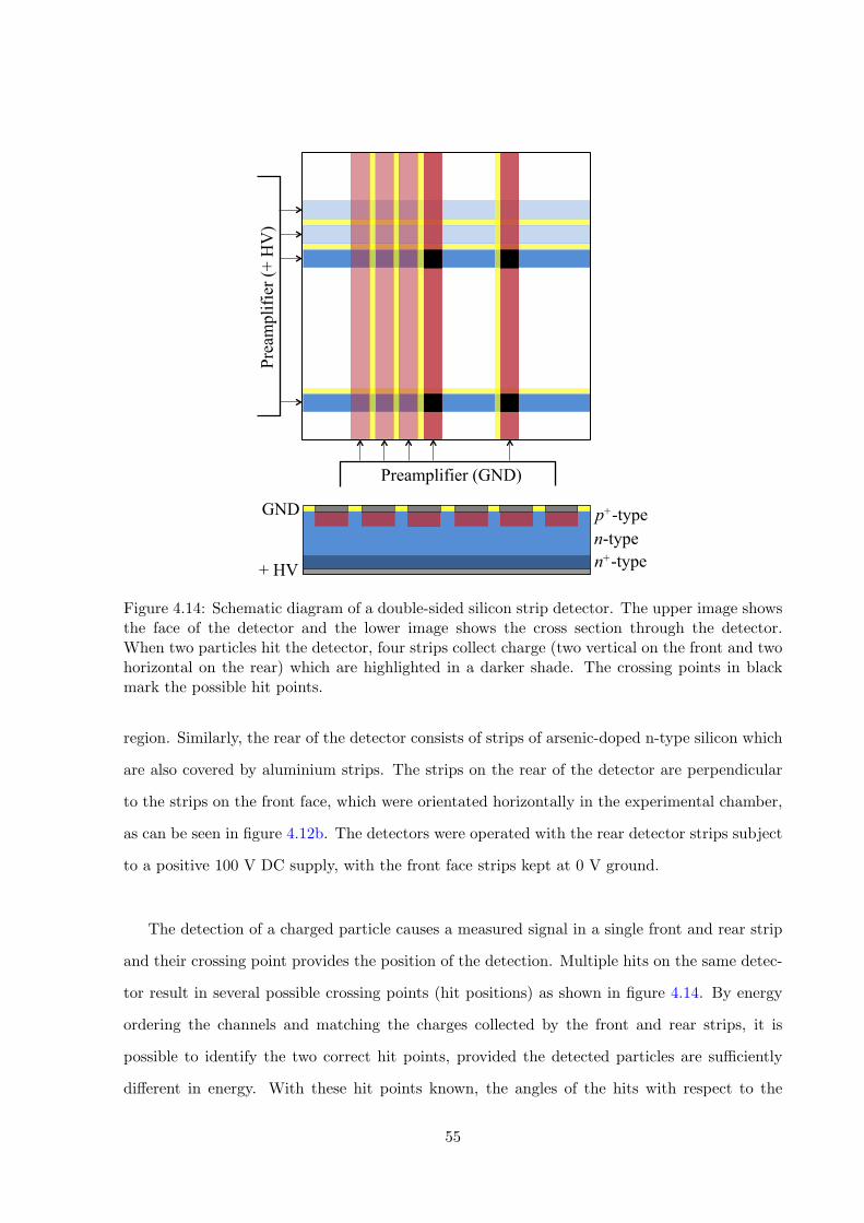
Preamplifier (GND)

n-type

+ HV

GND p+-type

n+-type

Prea

mpl

ifier

(+ H

V)

Figure 4.14: Schematic diagram of a double-sided silicon strip detector. The upper image showsthe face of the detector and the lower image shows the cross section through the detector.When two particles hit the detector, four strips collect charge (two vertical on the front and twohorizontal on the rear) which are highlighted in a darker shade. The crossing points in blackmark the possible hit points.

region. Similarly, the rear of the detector consists of strips of arsenic-doped n-type silicon which

are also covered by aluminium strips. The strips on the rear of the detector are perpendicular

to the strips on the front face, which were orientated horizontally in the experimental chamber,

as can be seen in figure 4.12b. The detectors were operated with the rear detector strips subject

to a positive 100 V DC supply, with the front face strips kept at 0 V ground.

The detection of a charged particle causes a measured signal in a single front and rear strip

and their crossing point provides the position of the detection. Multiple hits on the same detec-

tor result in several possible crossing points (hit positions) as shown in figure 4.14. By energy

ordering the channels and matching the charges collected by the front and rear strips, it is

possible to identify the two correct hit points, provided the detected particles are su�ciently

di↵erent in energy. With these hit points known, the angles of the hits with respect to the

55

beam direction and the target can be calculated using simple trigonometry as shown in figure

4.15. This is discussed in more detail in appendix B. Each strip has a width of 3mm, which,

when combined with the distances of the detectors from the target, leads to a ✓x and ✓y angular

resolution which ranges between 1.6� and 2.6�. The detected energy and these angles can be

used to determine the linear momentum vectors of each detected particle, assuming each to be

an ↵-particle.

The detectors were calibrated in energy using 148Gd and 241Am ↵ sources (energies of 3.2

and 5.5 MeV, respectively). The ↵-particle energies were not corrected for energy losses in the

dead layers of the detector since this was found to be very small compared with the intrinsic

resolution.

Figure 4.15: Notation for assigning the angle of the particle detection with respect to the initialbeam direction and the target. Image from reference [90].

56

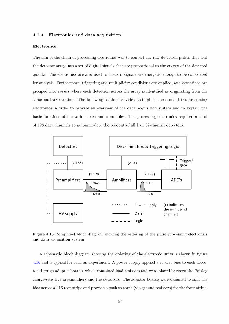
4.2.4 Electronics and data acquisition

Electronics

The aim of the chain of processing electronics was to convert the raw detection pulses that exit

the detector array into a set of digital signals that are proportional to the energy of the detected

quanta. The electronics are also used to check if signals are energetic enough to be considered

for analysis. Furthermore, triggering and multiplicity conditions are applied, and detections are

grouped into events where each detection across the array is identified as originating from the

same nuclear reaction. The following section provides a simplified account of the processing

electronics in order to provide an overview of the data acquisition system and to explain the

basic functions of the various electronics modules. The processing electronics required a total

of 128 data channels to accommodate the readout of all four 32-channel detectors.

Detectors

Preamplifiers Amplifiers

HVsupply

ADC’s

Discriminators&TriggeringLogic

(x128)

(x128)

(x64)

(x128)

Trigger/gate

Logic

Data

Powersupply (x)Indicatesthenumberofchannels

~50mV

~100μs

~1V

~1μs

Figure 4.16: Simplified block diagram showing the ordering of the pulse processing electronicsand data acquisition system.

A schematic block diagram showing the ordering of the electronic units is shown in figure

4.16 and is typical for such an experiment. A power supply applied a reverse bias to each detec-

tor through adapter boards, which contained load resistors and were placed between the Paisley

charge-sensitive preamplifiers and the detectors. The adaptor boards were designed to split the

bias across all 16 rear strips and provide a path to earth (via ground resistors) for the front strips.

57

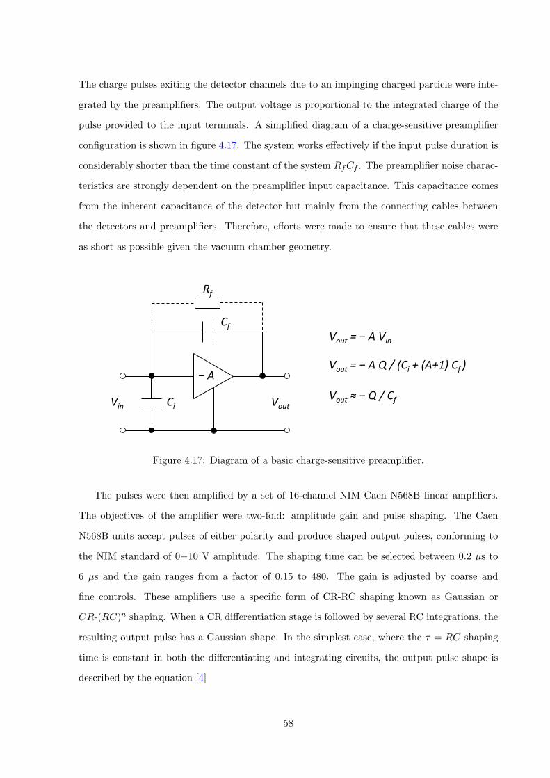
The charge pulses exiting the detector channels due to an impinging charged particle were inte-

grated by the preamplifiers. The output voltage is proportional to the integrated charge of the

pulse provided to the input terminals. A simplified diagram of a charge-sensitive preamplifier

configuration is shown in figure 4.17. The system works e↵ectively if the input pulse duration is

considerably shorter than the time constant of the system RfCf . The preamplifier noise charac-

teristics are strongly dependent on the preamplifier input capacitance. This capacitance comes

from the inherent capacitance of the detector but mainly from the connecting cables between

the detectors and preamplifiers. Therefore, e↵orts were made to ensure that these cables were

as short as possible given the vacuum chamber geometry.

Cf#

Rf#

Ci#Vin# Vout#

Vout#=#−#A#Vin#

Vout#=#−#A#Q#/#(Ci#+#(A+1)#Cf#)##−#A#Vout#≈#−#Q#/#Cf#

Figure 4.17: Diagram of a basic charge-sensitive preamplifier.

The pulses were then amplified by a set of 16-channel NIM Caen N568B linear amplifiers.

The objectives of the amplifier were two-fold: amplitude gain and pulse shaping. The Caen

N568B units accept pulses of either polarity and produce shaped output pulses, conforming to

the NIM standard of 0�10 V amplitude. The shaping time can be selected between 0.2 µs to

6 µs and the gain ranges from a factor of 0.15 to 480. The gain is adjusted by coarse and

fine controls. These amplifiers use a specific form of CR-RC shaping known as Gaussian or

CR-(RC)n shaping. When a CR di↵erentiation stage is followed by several RC integrations, the

resulting output pulse has a Gaussian shape. In the simplest case, where the ⌧ = RC shaping

time is constant in both the di↵erentiating and integrating circuits, the output pulse shape is

described by the equation [4]

58

Eout =

✓t

⌧

◆n

e�t/⌧ (4.3)

where n is the number of integration stages and t is the elapsed time. The output channels of the

amplifiers are split. The ⇥ 10 outputs were sent directly to the Silena S9418 analogue-to-digital

converters (ADCs) and the 1 ⇥ outputs were sent to the discriminators and triggering logic.

As explained, the set-up was subject to baseline electronic noise that primarily originates

from the circuit prior to the preamplifiers. To overcome this, and only consider signals which

correspond to particle detections, a system of four VME Caen V895 16-channel leading-edge

discriminators were employed. If an input exceeds a discriminator channel’s preset threshold

level, a 50 mV square-wave logic pulse is outputted. Since the channels on the front and the

back face of a detector originate from the same detection, the circuit was designed to only trigger

from the channels from the front faces of each detector.

The outputs from the discriminators were used in the triggering logic circuit shown in figure

4.18. The discriminators each have an or and a sum output. These can be used to trigger

the data acquisition in di↵erent ways. Connecting the sum outputs of the discriminators in a

daisy chain allows the total number of detections across the detector array to be evaluated. A

multiplicity condition was set for 3 or more coincident detections. If this is the case, a signal is

sent to a logic fan in / fan out (FI/FO) NIM unit. This outputs a logic pulse if any of its input

channels fire. At the same time, the or signal from the discriminators can be sent to another

FI/FO. This FI/FO outputs a logic pulse if any detector in the array is found to fire. This

singles trigger rate is scaled-down by a factor of 1000 using a rate divider unit (only 1/1000

inputs lead to an output from this unit). The scaled-down signal along with the multiplicity 3

signal are then sent to another FI/FO which produces the trigger for the ADCs.

The trigger signal has the purpose of notifying the ADCs of the forthcoming arrival of the

energy signals from the amplifiers. Following the receipt of the trigger, the ADC modules

are alert for 5 µs. All signals arriving within this time window are processed by the ADC

59

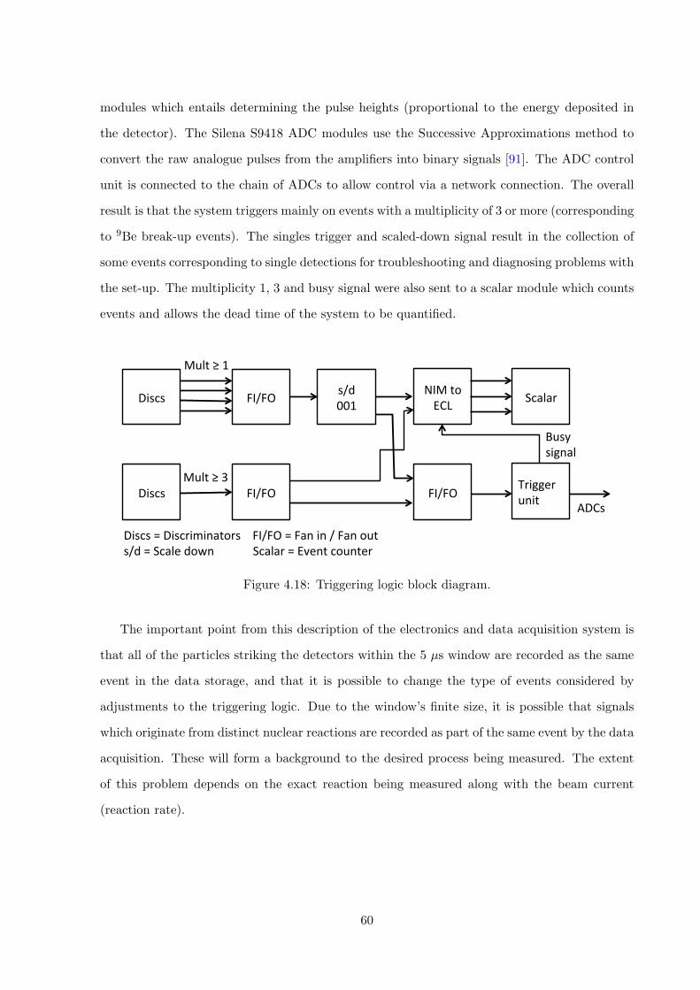
modules which entails determining the pulse heights (proportional to the energy deposited in

the detector). The Silena S9418 ADC modules use the Successive Approximations method to

convert the raw analogue pulses from the amplifiers into binary signals [91]. The ADC control

unit is connected to the chain of ADCs to allow control via a network connection. The overall

result is that the system triggers mainly on events with a multiplicity of 3 or more (corresponding

to 9Be break-up events). The singles trigger and scaled-down signal result in the collection of

some events corresponding to single detections for troubleshooting and diagnosing problems with

the set-up. The multiplicity 1, 3 and busy signal were also sent to a scalar module which counts

events and allows the dead time of the system to be quantified.

Discs

Discs

FI/FO

FI/FO

s/d001

NIMtoECL

FI/FO

Scalar

Busysignal

Triggerunit

Mult≥1

Mult≥3

Discs=DiscriminatorsFI/FO=Fanin/Fanouts/d=ScaledownScalar=Eventcounter

ADCs

Figure 4.18: Triggering logic block diagram.

The important point from this description of the electronics and data acquisition system is

that all of the particles striking the detectors within the 5 µs window are recorded as the same

event in the data storage, and that it is possible to change the type of events considered by

adjustments to the triggering logic. Due to the window’s finite size, it is possible that signals

which originate from distinct nuclear reactions are recorded as part of the same event by the data

acquisition. These will form a background to the desired process being measured. The extent

of this problem depends on the exact reaction being measured along with the beam current

(reaction rate).

60

Data acquisition and analysis software

The data acquisition software used was called MIDAS (Multi Instance Data Acquisition System)

[92]. The software system includes a Graphical User Interface and hardware control servers.

Although MIDAS has a built-in data analysis and sorting capability, this was performed

externally using SUNSORT [93]. The Sunsort documentation states: ”At the heart of the Sun-

sort package is a library of C functions which provides the user with facilities to access data

... and to decode this data into a simple array of ADC values. A user provided FORTRAN or

C subroutine is linked to this library to form the core sort process. During sorting, the user’s

subroutine is called once per event and is passed the array containing the ADC values. The user

can call upon various Sunsort library utility routines in order to, amongst other things, incre-

ment spectra, perform windowing operations and filter selected events back to a storage medium.”

A Fortran sort code was written to perform the primary data analysis, detailed in section

4.3. The sorting process involves determining if events correspond to the desired reaction and

where this is the case, constructing a 9Be excitation spectrum for these events.

61

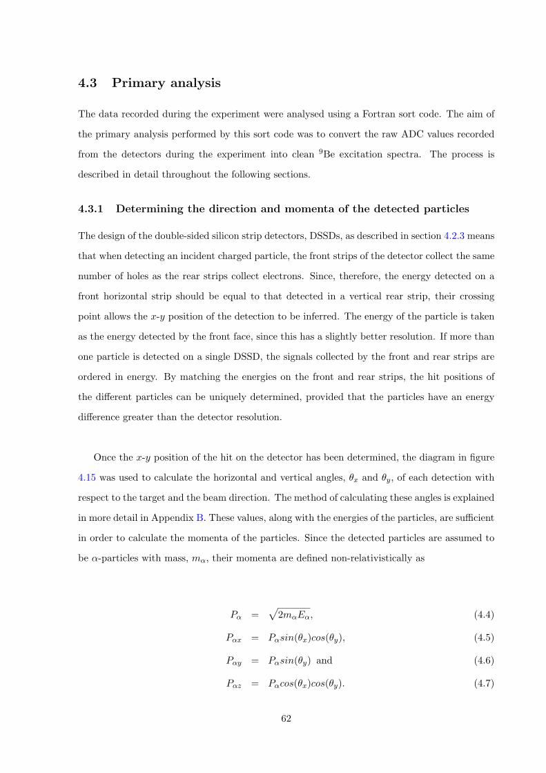
4.3 Primary analysis

The data recorded during the experiment were analysed using a Fortran sort code. The aim of

the primary analysis performed by this sort code was to convert the raw ADC values recorded

from the detectors during the experiment into clean 9Be excitation spectra. The process is

described in detail throughout the following sections.

4.3.1 Determining the direction and momenta of the detected particles

The design of the double-sided silicon strip detectors, DSSDs, as described in section 4.2.3 means

that when detecting an incident charged particle, the front strips of the detector collect the same

number of holes as the rear strips collect electrons. Since, therefore, the energy detected on a

front horizontal strip should be equal to that detected in a vertical rear strip, their crossing

point allows the x-y position of the detection to be inferred. The energy of the particle is taken

as the energy detected by the front face, since this has a slightly better resolution. If more than

one particle is detected on a single DSSD, the signals collected by the front and rear strips are

ordered in energy. By matching the energies on the front and rear strips, the hit positions of

the di↵erent particles can be uniquely determined, provided that the particles have an energy

di↵erence greater than the detector resolution.

Once the x-y position of the hit on the detector has been determined, the diagram in figure

4.15 was used to calculate the horizontal and vertical angles, ✓x and ✓y, of each detection with

respect to the target and the beam direction. The method of calculating these angles is explained

in more detail in Appendix B. These values, along with the energies of the particles, are su�cient

in order to calculate the momenta of the particles. Since the detected particles are assumed to

be ↵-particles with mass, m↵, their momenta are defined non-relativistically as

P↵ =p

2m↵E↵, (4.4)

P↵x = P↵sin(✓x)cos(✓y), (4.5)

P↵y = P↵sin(✓y) and (4.6)

P↵z = P↵cos(✓x)cos(✓y). (4.7)

62

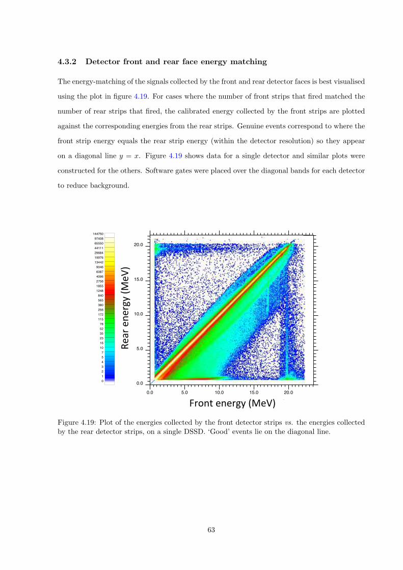
4.3.2 Detector front and rear face energy matching

The energy-matching of the signals collected by the front and rear detector faces is best visualised

using the plot in figure 4.19. For cases where the number of front strips that fired matched the

number of rear strips that fired, the calibrated energy collected by the front strips are plotted

against the corresponding energies from the rear strips. Genuine events correspond to where the

front strip energy equals the rear strip energy (within the detector resolution) so they appear

on a diagonal line y = x. Figure 4.19 shows data for a single detector and similar plots were

constructed for the others. Software gates were placed over the diagonal bands for each detector

to reduce background.

144750974086555044111296841997613442

904660874096275618551248

840565380256172115

785235231610

7543210

0.0

5.0

10.0

15.0

20.0

25.0

0.0 5.0 10.0 15.0 20.0 25.0

Rea

r ene

rgy

(MeV

)

Front energy (MeV)

144750974086555044111296841997613442

904660874096275618551248

840565380256172115

785235231610

7543210

0.0

5.0

10.0

15.0

20.0

25.0

0.0 5.0 10.0 15.0 20.0 25.0

Rea

r ene

rgy

(MeV

)

Front energy (MeV)Frontenergy(MeV)

Rearene

rgy(M

eV)

144750974086555044111296841997613442

904660874096275618551248

840565380256172115

785235231610

7543210

0.0

5.0

10.0

15.0

20.0

25.0

0.0 5.0 10.0 15.0 20.0 25.0

Rea

r ene

rgy

(MeV

)

Front energy (MeV)

144750974086555044111296841997613442

904660874096275618551248

840565380256172115

785235231610

7543210

0.0

5.0

10.0

15.0

20.0

25.0

0.0 5.0 10.0 15.0 20.0 25.0

Rea

r ene

rgy

(MeV

)

Front energy (MeV)Figure 4.19: Plot of the energies collected by the front detector strips vs. the energies collectedby the rear detector strips, on a single DSSD. ‘Good’ events lie on the diagonal line.

63

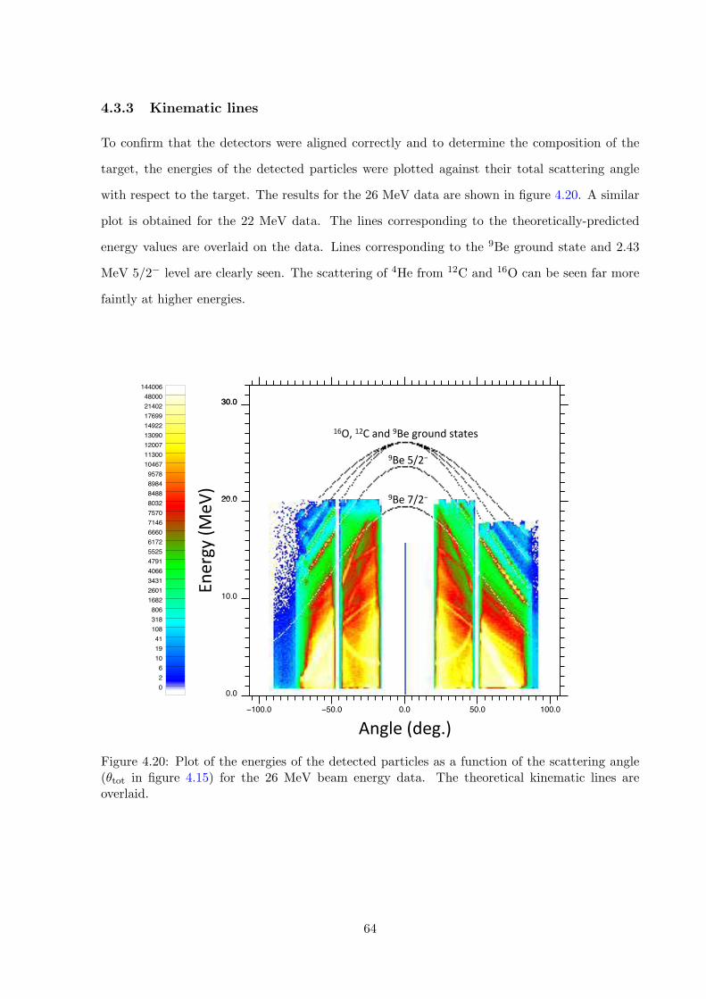
4.3.3 Kinematic lines

To confirm that the detectors were aligned correctly and to determine the composition of the

target, the energies of the detected particles were plotted against their total scattering angle

with respect to the target. The results for the 26 MeV data are shown in figure 4.20. A similar

plot is obtained for the 22 MeV data. The lines corresponding to the theoretically-predicted

energy values are overlaid on the data. Lines corresponding to the 9Be ground state and 2.43

MeV 5/2� level are clearly seen. The scattering of 4He from 12C and 16O can be seen far more

faintly at higher energies.144006

4800021402176991492213090120071130010467

95788984848880327570714666606172552547914066343126011682

806318108

411910

620

0.0

10.0

20.0

30.0

−100.0 −50.0 0.0 50.0 100.0

Ener

gy (M

eV)

Angle (deg.)

24000240200166140114

95806655463932272218151413121110

9876543210

0.0

10.0

20.0

30.0

−100.0 −50.0 0.0 50.0 100.0

Ener

gy (M

eV)

Angle (deg.)

24000240200166140114

95806655463932272218151413121110

9876543210

0.0

10.0

20.0

30.0

−100.0 −50.0 0.0 50.0 100.0

Ener

gy (M

eV)

Angle (deg.)

24000240200166140114

95806655463932272218151413121110

9876543210

0.0

10.0

20.0

30.0

−100.0 −50.0 0.0 50.0 100.0

Ener

gy (M

eV)

Angle (deg.)

16O,12Cand9Begroundstates

9Be5/2−

9Be7/2−

1440064800021402176991492213090120071130010467

95788984848880327570714666606172552547914066343126011682

806318108

411910

620

0.0

10.0

20.0

30.0

−100.0 −50.0 0.0 50.0 100.0

Ener

gy (M

eV)

Angle (deg.)Angle(deg.)

Energy(M

eV)

Figure 4.20: Plot of the energies of the detected particles as a function of the scattering angle(✓tot in figure 4.15) for the 26 MeV beam energy data. The theoretical kinematic lines areoverlaid.

64

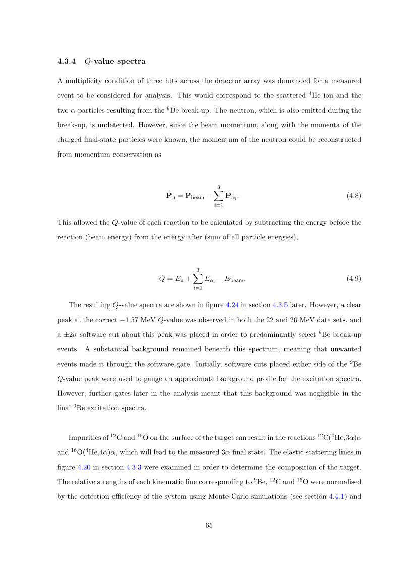
4.3.4 Q-value spectra

A multiplicity condition of three hits across the detector array was demanded for a measured

event to be considered for analysis. This would correspond to the scattered 4He ion and the

two ↵-particles resulting from the 9Be break-up. The neutron, which is also emitted during the

break-up, is undetected. However, since the beam momentum, along with the momenta of the

charged final-state particles were known, the momentum of the neutron could be reconstructed

from momentum conservation as

Pn = Pbeam �3X

i=1

P↵i

. (4.8)

This allowed the Q-value of each reaction to be calculated by subtracting the energy before the

reaction (beam energy) from the energy after (sum of all particle energies),

Q = En +3X

i=1

E↵i

� Ebeam. (4.9)

The resulting Q-value spectra are shown in figure 4.24 in section 4.3.5 later. However, a clear

peak at the correct �1.57 MeV Q-value was observed in both the 22 and 26 MeV data sets, and

a ±2� software cut about this peak was placed in order to predominantly select 9Be break-up

events. A substantial background remained beneath this spectrum, meaning that unwanted

events made it through the software gate. Initially, software cuts placed either side of the 9Be

Q-value peak were used to gauge an approximate background profile for the excitation spectra.

However, further gates later in the analysis meant that this background was negligible in the

final 9Be excitation spectra.

Impurities of 12C and 16O on the surface of the target can result in the reactions 12C(4He,3↵)↵

and 16O(4He,4↵)↵, which will lead to the measured 3↵ final state. The elastic scattering lines in

figure 4.20 in section 4.3.3 were examined in order to determine the composition of the target.

The relative strengths of each kinematic line corresponding to 9Be, 12C and 16O were normalised

by the detection e�ciency of the system using Monte-Carlo simulations (see section 4.4.1) and

65

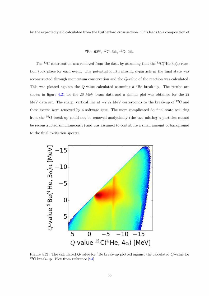
by the expected yield calculated from the Rutherford cross section. This leads to a composition of

9Be: 92%, 12C: 6%, 16O: 2%.

The 12C contribution was removed from the data by assuming that the 12C(4He,3↵)↵ reac-

tion took place for each event. The potential fourth missing ↵-particle in the final state was

reconstructed through momentum conservation and the Q-value of the reaction was calculated.

This was plotted against the Q-value calculated assuming a 9Be break-up. The results are

shown in figure 4.21 for the 26 MeV beam data and a similar plot was obtained for the 22

MeV data set. The sharp, vertical line at �7.27 MeV corresponds to the break-up of 12C and

these events were removed by a software gate. The more complicated 5↵ final state resulting

from the 16O break-up could not be removed analytically (the two missing ↵-particles cannot

be reconstructed simultaneously) and was assumed to contribute a small amount of background

to the final excitation spectra.

Figure 4.21: The calculated Q-value for 9Be break-up plotted against the calculated Q-value for12C break-up. Plot from reference [94].

66

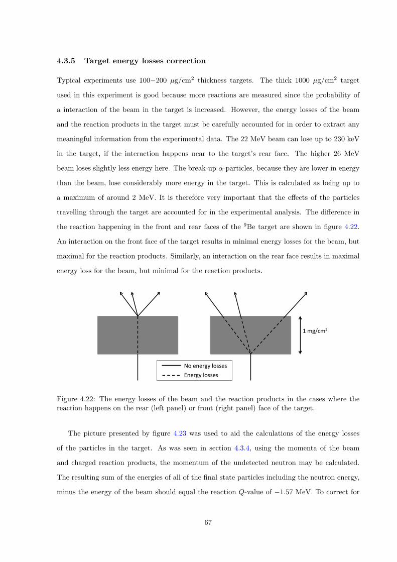
4.3.5 Target energy losses correction

Typical experiments use 100�200 µg/cm2 thickness targets. The thick 1000 µg/cm2 target

used in this experiment is good because more reactions are measured since the probability of

a interaction of the beam in the target is increased. However, the energy losses of the beam

and the reaction products in the target must be carefully accounted for in order to extract any

meaningful information from the experimental data. The 22 MeV beam can lose up to 230 keV

in the target, if the interaction happens near to the target’s rear face. The higher 26 MeV

beam loses slightly less energy here. The break-up ↵-particles, because they are lower in energy

than the beam, lose considerably more energy in the target. This is calculated as being up to

a maximum of around 2 MeV. It is therefore very important that the e↵ects of the particles

travelling through the target are accounted for in the experimental analysis. The di↵erence in

the reaction happening in the front and rear faces of the 9Be target are shown in figure 4.22.

An interaction on the front face of the target results in minimal energy losses for the beam, but

maximal for the reaction products. Similarly, an interaction on the rear face results in maximal

energy loss for the beam, but minimal for the reaction products.

1mg/cm2

NoenergylossesEnergylosses

Figure 4.22: The energy losses of the beam and the reaction products in the cases where thereaction happens on the rear (left panel) or front (right panel) face of the target.

The picture presented by figure 4.23 was used to aid the calculations of the energy losses

of the particles in the target. As was seen in section 4.3.4, using the momenta of the beam

and charged reaction products, the momentum of the undetected neutron may be calculated.

The resulting sum of the energies of all of the final state particles including the neutron energy,

minus the energy of the beam should equal the reaction Q-value of �1.57 MeV. To correct for

67

the energy losses of the particles, an iterative technique was developed. In the calculations,

the value of D in figure 4.23 was incremented between the front and rear faces of the target

(10 iterations were included). For each value of D, the energy loss of the beam was calculated

and the energy at the interaction point E0b was evaluated. How the energy losses were actually

calculated is discussed shortly.

T

D

Eb

Eb’

Eα1 Eα2 Eα3En

Ei’

Figure 4.23: Diagram used to numerically calculate the energy losses of the particles in thetarget.

Based on the measured angles ✓ of all of the charged reaction products, the total dis-

tance through the target they travelled, based on the interaction point, D, were calculated

as d = (T �D)/cos(✓). Given their measured energies and the distances they travelled through

the target, their initial energies at the interaction point were calculated. The reduced beam

energy and the corrected ↵-particle energies were used to calculate the energy of the undetected

neutron. The total energy of the final state particles was then evaluated and the reaction Q-

value added. This should result in the calculation of the reduced beam energy at the interaction

point. This quantity was calculated for all iterations of the interaction distance D, and the point

that most closely reproduced the correct beam energy was chosen as the interaction point.

To illustrate the improvement that this process provides, figure 4.24 shows the measured

Q-value spectra for the reactions, before and after the energy-loss routine was implemented. A

substantial improvement in the resolution of the Q-value was seen for both the 22 MeV and

26 MeV data sets. Figure 4.25 demonstrates the e↵ect of the energy-loss corrections on the

calculated excitation energies of 9Be.

68

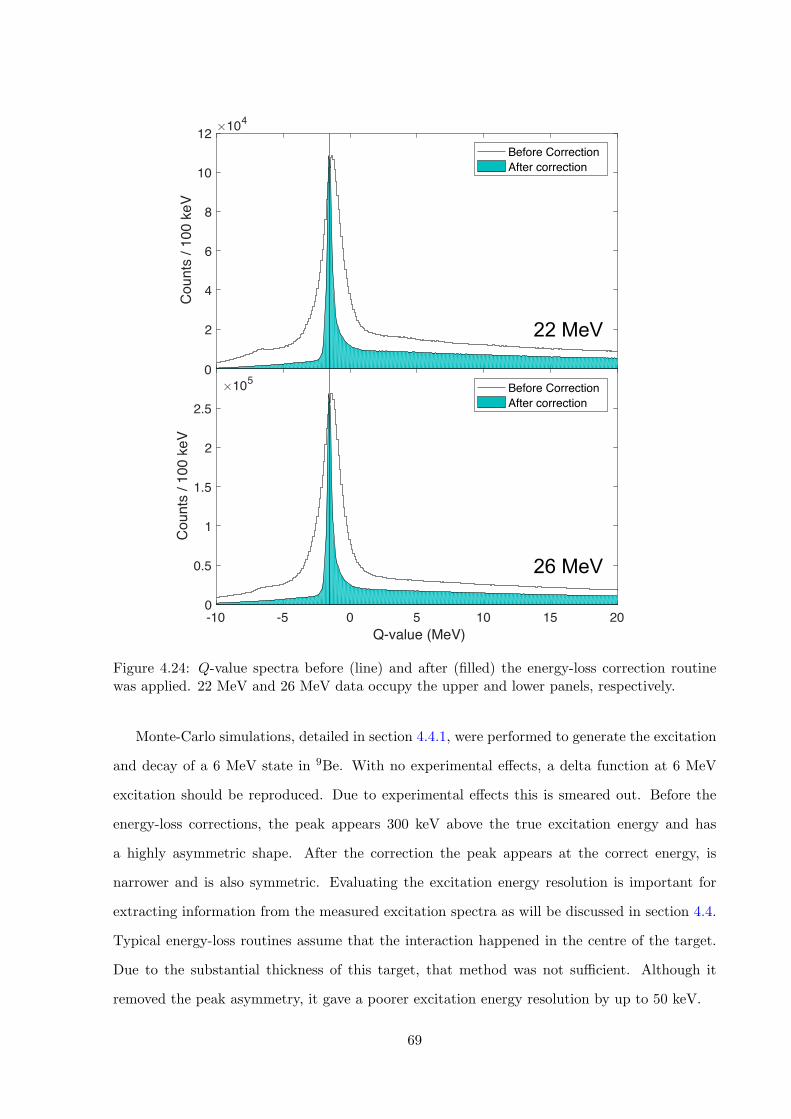
-10 -5 0 5 10 15 20Q-value (MeV)

0

0.5

1

1.5

2

2.5

3

Cou

nts

/ 100

keV

�105

Before CorrectionAfter correction

-10 -5 0 5 10 15 20Q-value (MeV)

0

0.5

1

1.5

2

2.5

3

Cou

nts

/ 100

keV

�105

Before CorrectionAfter correction

-10 -5 0 5 10 15 20Q-value (MeV)

0

2

4

6

8

10

12

Cou

nts

/ 100

keV

�104

Before CorrectionAfter correction

-10 -5 0 5 10 15 20Q-value (MeV)

0

2

4

6

8

10

12

Cou

nts

/ 100

keV

�104

Before CorrectionAfter correction

22 MeV

26 MeV

Figure 4.24: Q-value spectra before (line) and after (filled) the energy-loss correction routinewas applied. 22 MeV and 26 MeV data occupy the upper and lower panels, respectively.

Monte-Carlo simulations, detailed in section 4.4.1, were performed to generate the excitation

and decay of a 6 MeV state in 9Be. With no experimental e↵ects, a delta function at 6 MeV

excitation should be reproduced. Due to experimental e↵ects this is smeared out. Before the

energy-loss corrections, the peak appears 300 keV above the true excitation energy and has

a highly asymmetric shape. After the correction the peak appears at the correct energy, is

narrower and is also symmetric. Evaluating the excitation energy resolution is important for

extracting information from the measured excitation spectra as will be discussed in section 4.4.

Typical energy-loss routines assume that the interaction happened in the centre of the target.

Due to the substantial thickness of this target, that method was not su�cient. Although it

removed the peak asymmetry, it gave a poorer excitation energy resolution by up to 50 keV.

69

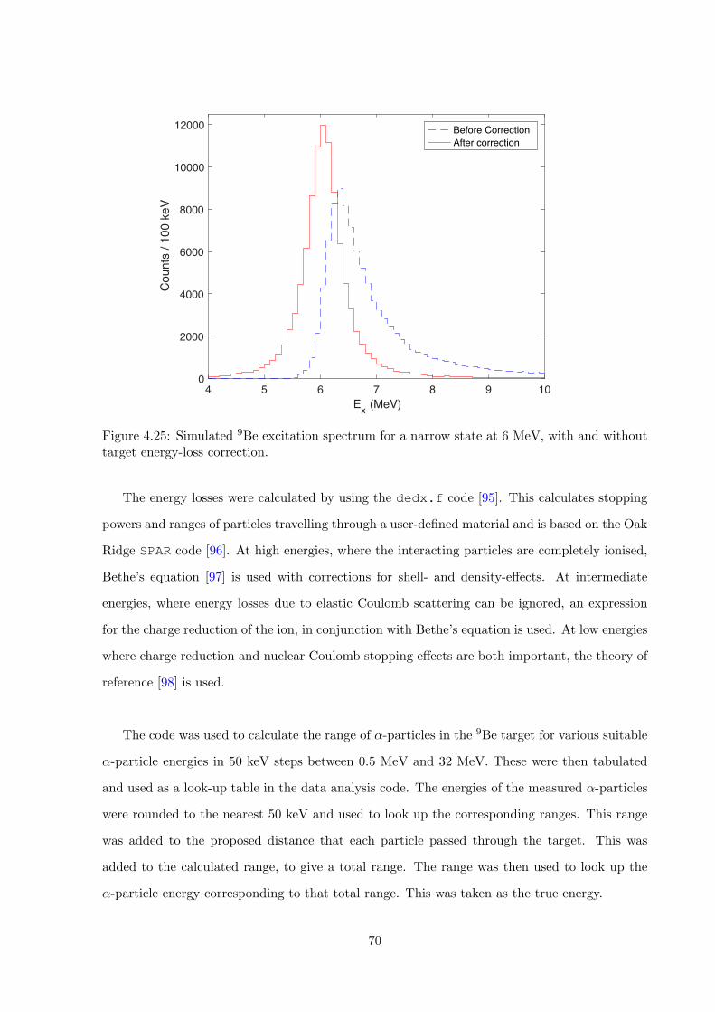
4 5 6 7 8 9 10Ex (MeV)

0

2000

4000

6000

8000

10000

12000

Cou

nts

/ 100

keV

Before CorrectionAfter correction

Figure 4.25: Simulated 9Be excitation spectrum for a narrow state at 6 MeV, with and withouttarget energy-loss correction.

The energy losses were calculated by using the dedx.f code [95]. This calculates stopping

powers and ranges of particles travelling through a user-defined material and is based on the Oak

Ridge SPAR code [96]. At high energies, where the interacting particles are completely ionised,

Bethe’s equation [97] is used with corrections for shell- and density-e↵ects. At intermediate

energies, where energy losses due to elastic Coulomb scattering can be ignored, an expression

for the charge reduction of the ion, in conjunction with Bethe’s equation is used. At low energies

where charge reduction and nuclear Coulomb stopping e↵ects are both important, the theory of

reference [98] is used.

The code was used to calculate the range of ↵-particles in the 9Be target for various suitable

↵-particle energies in 50 keV steps between 0.5 MeV and 32 MeV. These were then tabulated

and used as a look-up table in the data analysis code. The energies of the measured ↵-particles

were rounded to the nearest 50 keV and used to look up the corresponding ranges. This range

was added to the proposed distance that each particle passed through the target. This was

added to the calculated range, to give a total range. The range was then used to look up the

↵-particle energy corresponding to that total range. This was taken as the true energy.

70

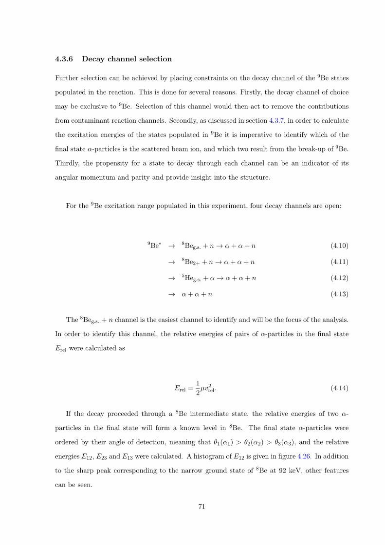
4.3.6 Decay channel selection

Further selection can be achieved by placing constraints on the decay channel of the 9Be states

populated in the reaction. This is done for several reasons. Firstly, the decay channel of choice

may be exclusive to 9Be. Selection of this channel would then act to remove the contributions

from contaminant reaction channels. Secondly, as discussed in section 4.3.7, in order to calculate

the excitation energies of the states populated in 9Be it is imperative to identify which of the

final state ↵-particles is the scattered beam ion, and which two result from the break-up of 9Be.

Thirdly, the propensity for a state to decay through each channel can be an indicator of its

angular momentum and parity and provide insight into the structure.

For the 9Be excitation range populated in this experiment, four decay channels are open:

9Be⇤ ! 8Beg.s. + n ! ↵+ ↵+ n (4.10)

! 8Be2+ + n ! ↵+ ↵+ n (4.11)

! 5Heg.s. + ↵! ↵+ ↵+ n (4.12)

! ↵+ ↵+ n (4.13)

The 8Beg.s. + n channel is the easiest channel to identify and will be the focus of the analysis.

In order to identify this channel, the relative energies of pairs of ↵-particles in the final state

Erel were calculated as

Erel =1

2µv2rel. (4.14)

If the decay proceeded through a 8Be intermediate state, the relative energies of two ↵-

particles in the final state will form a known level in 8Be. The final state ↵-particles were

ordered by their angle of detection, meaning that ✓1(↵1) > ✓2(↵2) > ✓3(↵3), and the relative

energies E12, E23 and E13 were calculated. A histogram of E12 is given in figure 4.26. In addition

to the sharp peak corresponding to the narrow ground state of 8Be at 92 keV, other features

can be seen.

71

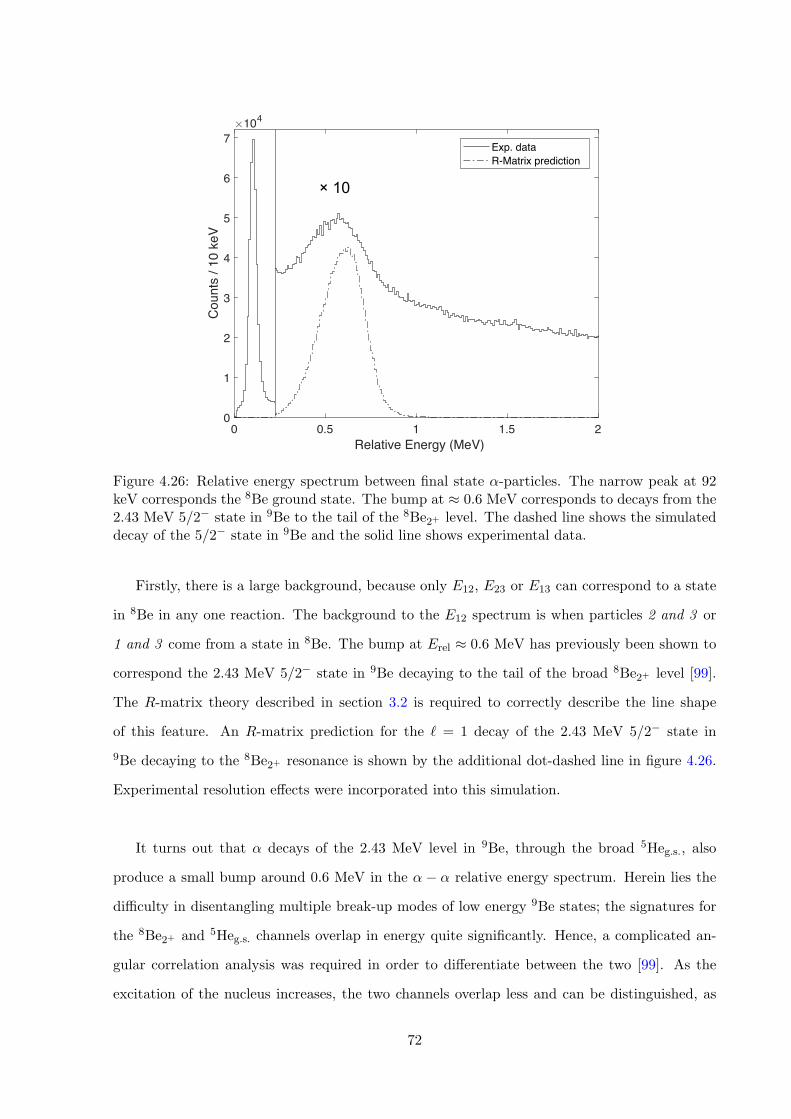
0 0.5 1 1.5 2Relative Energy (MeV)

0

1

2

3

4

5

6

7

Cou

nts

/ 10

keV

Exp. dataR-Matrix prediction

0 0.5 1 1.5 2Relative Energy (MeV)

0

1

2

3

4

5

6

7

Cou

nts

/ 10

keV

�104

Exp. dataR-Matrix prediction

× 10

Figure 4.26: Relative energy spectrum between final state ↵-particles. The narrow peak at 92keV corresponds the 8Be ground state. The bump at ⇡ 0.6 MeV corresponds to decays from the2.43 MeV 5/2� state in 9Be to the tail of the 8Be2+ level. The dashed line shows the simulateddecay of the 5/2� state in 9Be and the solid line shows experimental data.

Firstly, there is a large background, because only E12, E23 or E13 can correspond to a state

in 8Be in any one reaction. The background to the E12 spectrum is when particles 2 and 3 or

1 and 3 come from a state in 8Be. The bump at Erel ⇡ 0.6 MeV has previously been shown to

correspond the 2.43 MeV 5/2� state in 9Be decaying to the tail of the broad 8Be2+ level [99].

The R-matrix theory described in section 3.2 is required to correctly describe the line shape

of this feature. An R-matrix prediction for the ` = 1 decay of the 2.43 MeV 5/2� state in

9Be decaying to the 8Be2+ resonance is shown by the additional dot-dashed line in figure 4.26.

Experimental resolution e↵ects were incorporated into this simulation.

It turns out that ↵ decays of the 2.43 MeV level in 9Be, through the broad 5Heg.s., also

produce a small bump around 0.6 MeV in the ↵ � ↵ relative energy spectrum. Herein lies the

di�culty in disentangling multiple break-up modes of low energy 9Be states; the signatures for

the 8Be2+ and 5Heg.s. channels overlap in energy quite significantly. Hence, a complicated an-

gular correlation analysis was required in order to di↵erentiate between the two [99]. As the

excitation of the nucleus increases, the two channels overlap less and can be distinguished, as

72

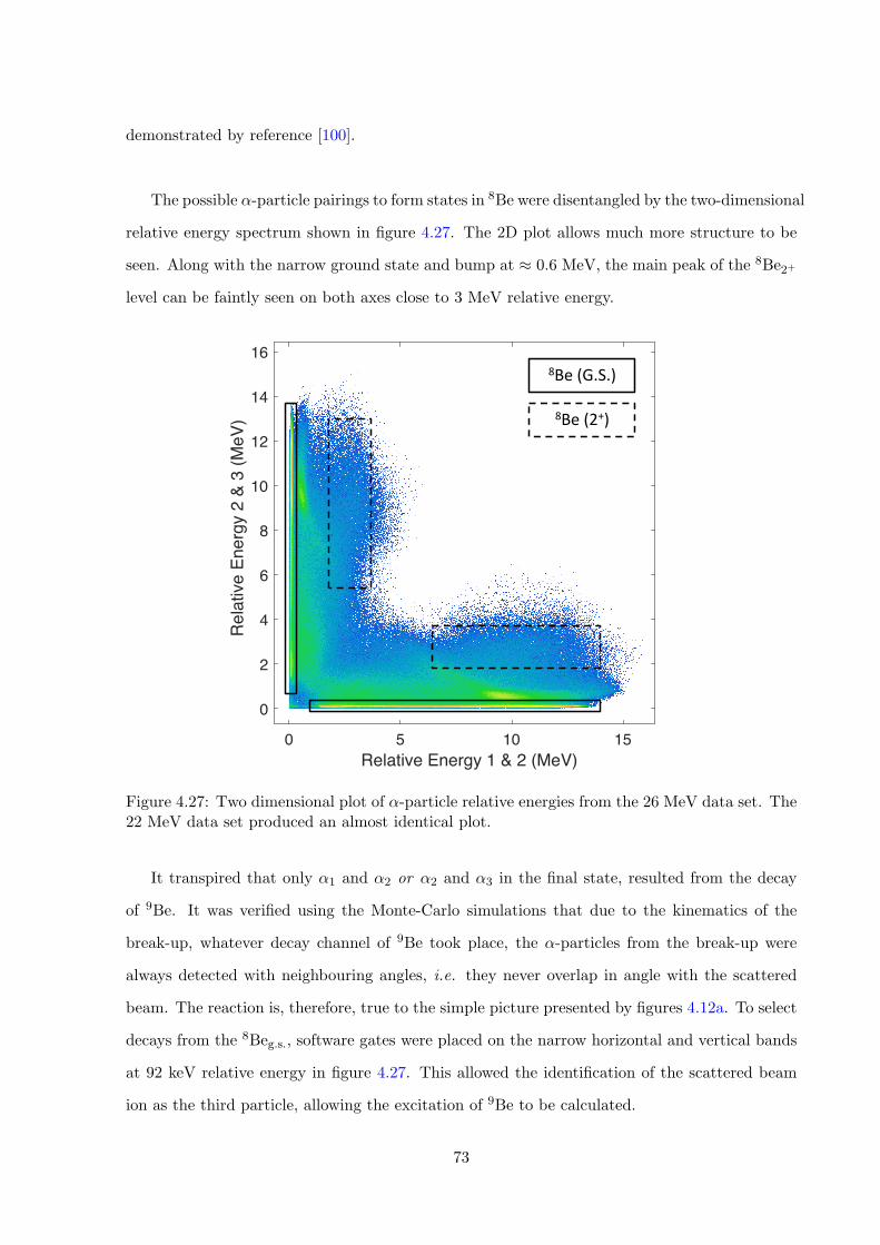
demonstrated by reference [100].

The possible ↵-particle pairings to form states in 8Be were disentangled by the two-dimensional

relative energy spectrum shown in figure 4.27. The 2D plot allows much more structure to be

seen. Along with the narrow ground state and bump at ⇡ 0.6 MeV, the main peak of the 8Be2+

level can be faintly seen on both axes close to 3 MeV relative energy.

0 5 10 15Relative Energy 1 & 2 (MeV)

0

2

4

6

8

10

12

14

16

Rel

ativ

e En

ergy

2 &

3 (M

eV)

8Be(G.S.)

8Be(2+)

Figure 4.27: Two dimensional plot of ↵-particle relative energies from the 26 MeV data set. The22 MeV data set produced an almost identical plot.

It transpired that only ↵1 and ↵2 or ↵2 and ↵3 in the final state, resulted from the decay

of 9Be. It was verified using the Monte-Carlo simulations that due to the kinematics of the

break-up, whatever decay channel of 9Be took place, the ↵-particles from the break-up were

always detected with neighbouring angles, i.e. they never overlap in angle with the scattered

beam. The reaction is, therefore, true to the simple picture presented by figures 4.12a. To select

decays from the 8Beg.s., software gates were placed on the narrow horizontal and vertical bands

at 92 keV relative energy in figure 4.27. This allowed the identification of the scattered beam

ion as the third particle, allowing the excitation of 9Be to be calculated.

73

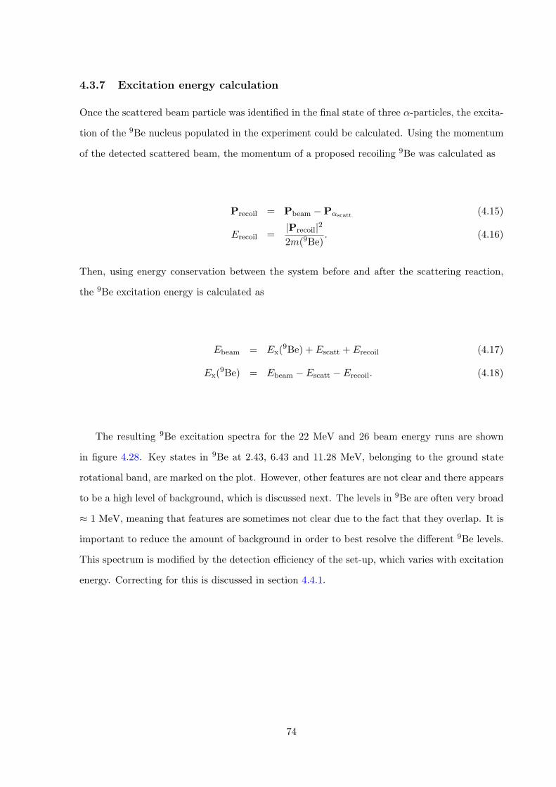
4.3.7 Excitation energy calculation

Once the scattered beam particle was identified in the final state of three ↵-particles, the excita-

tion of the 9Be nucleus populated in the experiment could be calculated. Using the momentum

of the detected scattered beam, the momentum of a proposed recoiling 9Be was calculated as

Precoil = Pbeam �P↵scatt

(4.15)

Erecoil =|Precoil|22m(9Be)

. (4.16)

Then, using energy conservation between the system before and after the scattering reaction,

the 9Be excitation energy is calculated as

Ebeam = Ex(9Be) + Escatt + Erecoil (4.17)

Ex(9Be) = Ebeam � Escatt � Erecoil. (4.18)

The resulting 9Be excitation spectra for the 22 MeV and 26 beam energy runs are shown

in figure 4.28. Key states in 9Be at 2.43, 6.43 and 11.28 MeV, belonging to the ground state

rotational band, are marked on the plot. However, other features are not clear and there appears

to be a high level of background, which is discussed next. The levels in 9Be are often very broad

⇡ 1 MeV, meaning that features are sometimes not clear due to the fact that they overlap. It is

important to reduce the amount of background in order to best resolve the di↵erent 9Be levels.

This spectrum is modified by the detection e�ciency of the set-up, which varies with excitation

energy. Correcting for this is discussed in section 4.4.1.

74

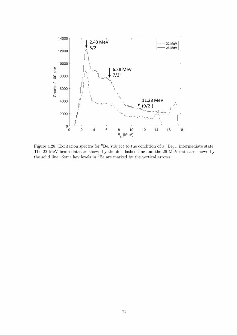
0 2 4 6 8 10 12 14 16 18Ex (MeV)

0

2000

4000

6000

8000

10000

12000

14000

Cou

nts

/ 100

keV

22 MeV26 MeV

2.43MeV5/2−

6.38MeV7/2−

11.28MeV(9/2−)

Figure 4.28: Excitation spectra for 9Be, subject to the condition of a 8Beg.s. intermediate state.The 22 MeV beam data are shown by the dot-dashed line and the 26 MeV data are shown bythe solid line. Some key levels in 9Be are marked by the vertical arrows.

75

4.3.8 Further contaminant reaction channels

The discussion in section 4.3.4 described how interactions with 12C contaminants in the target

were removed from the analysis. However, even when just considering the 4He + 9Be interaction,

there are reaction channels other than inelastic scattering that have to be accounted for. These

include the 9Be(4He,12C*)n reaction, populating states in 12C, and the 9Be(4He,5Heg.s.)8Beg.s.

neutron transfer reaction. To remove these contributions from the 9Be spectrum, the Dalitz plot

in figure 4.29 was constructed. This is shown for the 26 MeV data set, but the same analysis

was performed for the 22 MeV beam data.

6 8 10 12 14 16 18 20 22 24Ex Carbon-12 (MeV)

0

2

4

6

8

10

12

14

16

18

20

E x Ber

ylliu

m-9

(MeV

)

9Be(4He,12C)n9Be(4He,5Heg.s.)8Beg.s.

Figure 4.29: Excitation energy of a proposed 9Be (↵ + ↵ + n) vs. the excitation energy of aproposed 12C (↵ + ↵ + ↵) (26 MeV beam data only). Broad horizontal lines correspond tostates in 9Be and the vertical lines correspond to the known natural parity states in 12C. Thediagonal band corresponds to the neutron transfer reaction and break-up of 5He. The dashedand dot-dashed lines mark the regions occupied by contaminant reactions. See text for details.

Here, the excitation energy in 9Be, calculated in section 4.3.7 is plotted against an excitation

energy in 12C calculated from the three final state ↵-particles. The momentum and energy of

the proposed 12C were calculated as

76

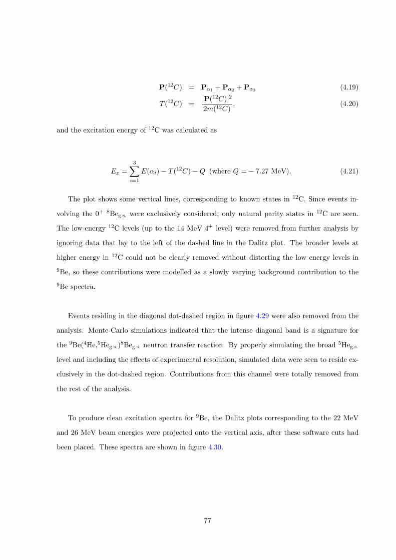
P(12C) = P↵1

+P↵2

+P↵3

(4.19)

T (12C) =|P(12C)|22m(12C)

, (4.20)

and the excitation energy of 12C was calculated as

Ex =3X

i=1

E(↵i)� T (12C)�Q (where Q =� 7.27 MeV). (4.21)

The plot shows some vertical lines, corresponding to known states in 12C. Since events in-

volving the 0+ 8Beg.s. were exclusively considered, only natural parity states in 12C are seen.

The low-energy 12C levels (up to the 14 MeV 4+ level) were removed from further analysis by

ignoring data that lay to the left of the dashed line in the Dalitz plot. The broader levels at

higher energy in 12C could not be clearly removed without distorting the low energy levels in

9Be, so these contributions were modelled as a slowly varying background contribution to the

9Be spectra.

Events residing in the diagonal dot-dashed region in figure 4.29 were also removed from the

analysis. Monte-Carlo simulations indicated that the intense diagonal band is a signature for

the 9Be(4He,5Heg.s.)8Beg.s. neutron transfer reaction. By properly simulating the broad 5Heg.s.

level and including the e↵ects of experimental resolution, simulated data were seen to reside ex-

clusively in the dot-dashed region. Contributions from this channel were totally removed from

the rest of the analysis.

To produce clean excitation spectra for 9Be, the Dalitz plots corresponding to the 22 MeV

and 26 MeV beam energies were projected onto the vertical axis, after these software cuts had

been placed. These spectra are shown in figure 4.30.

77

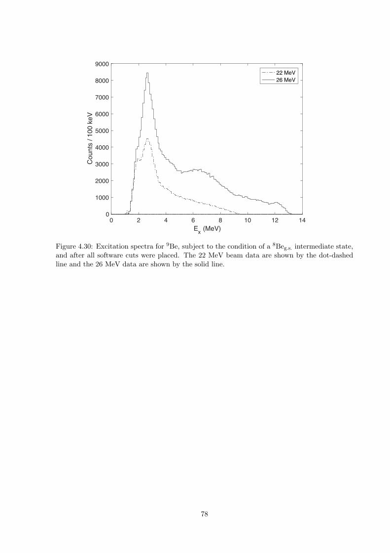
0 2 4 6 8 10 12 14Ex (MeV)

0

1000

2000

3000

4000

5000

6000

7000

8000

9000

Cou

nts

/ 100

keV

22 MeV26 MeV

Figure 4.30: Excitation spectra for 9Be, subject to the condition of a 8Beg.s. intermediate state,and after all software cuts were placed. The 22 MeV beam data are shown by the dot-dashedline and the 26 MeV data are shown by the solid line.

78

4.4 Secondary analysis

The secondary analysis consisted of three main stages. Firstly, the e↵ects of the experimental

resolution and e�ciency were investigated, through the use of Monte-Carlo simulations. These

e↵ects were then incorporated into the excitation spectra so that meaningful information could

be extracted from the data. Secondly, the experimental spectra were fit with resonance line

shapes to determine what states were populated in 9Be. Thirdly, the measured energies and

widths of the resonances were used to determine information such as their angular momentum

and parity, which may provide an insight into the nuclear structure.

4.4.1 Monte-Carlo simulations

Simulations were performed using the Resolution8 (RES8) Fortran 77 code, which is designed for

non-relativistic, thin-target experiments and can simulate various di↵erent types of reactions,

such as scattering, transfer and resonance. The code is unpublished but further details can be

found in references [101–103]. In its basic form, RES8 is a two-body kinematics code, so models

a break-up reaction as a chain of two-body decays, as shown in figure 4.31. The program allows

the user to define a beam nucleus, target nucleus, the break-up pathways, the excitation energy

of the particles produced in the reaction, the Q-values of each stage and the angular distribution

of the emitted particles.

A

B

C*

D

Q1

Q2 E

F*

Q3 G

H

*Indicatesapar.clethatwillbreakup

Figure 4.31: A sequential break-up reaction generated in RES8. A + B ! C⇤ +D then C⇤ !E + F⇤ etc.

In figure 4.31, where A is the target and B is the beam, the two-body kinematics for the first

reaction stage Q1 are generated for a scattering angle randomly sampled from a specified angular

79

distribution. The product C* is populated in an excited energy state defined by the user. A

state width can also be defined here, so that the populated excitation energy is sampled from a

distribution. Given the chosen scattering angle and excitation energy, the kinetic energies and

momenta of the C* and D particles are calculated. Break-up stages of either reaction product

can then be specified. Here C* breaks up into E and F*. In the centre-of-mass frame of C*,

given its excitation, and the Q-value, Q2, the energies of the fragments E and F* are then cal-

culated. Their angles with respect to the direction of the parent C* are sampled randomly from

a given probability distribution. These particles can then be boosted into the laboratory frame

using the momentum of C*. This process can be repeated for however many break-up stages are

required. The intermediate result is that the energies and directions of all final-state reaction

products in the laboratory frame are then known. Further e↵ects are included before this stage:

the beam energy can be smeared by a chosen distribution, and the beam systematically loses

some energy as it traverses a randomly-chosen depth into the target.

After this stage, the final state particles (here we have D, E, G and H) lose energy as they

exit the target from the beam depth. Their angular and energy straggle inside the target is also

calculated. Then, the positions and intrinsic energy resolution of each of the detectors are de-

fined. This then allows the detector pixel that each final state particle would hit to be identified

and the detector response to be calculated. The centre ✓x and ✓y angles of the strips that are

hit by each particle are chosen as the hit positions, and the particle energies are smeared by a

specified Gaussian energy resolution. The result is that the program outputs a set of energies

and angles of the final-state particles which include the e↵ects of the experimental set-up. These

data produced by RES8 are then analysed in the same way as the experimental data, in order

to account for any software cuts placed in the experimental data analysis.

The simulated data are used for three main reasons. Firstly, the various kinematical software

cuts used to focus cleanly on measuring 9Be break-ups rely on analysing the manifestation of

contaminant reaction channels on each of the experimental plots (see section 4.3.8). Using

the Monte-Carlo code allows the signature for each separate process to be identified, and to be

removed from the analysis of the 9Be scattering reaction. Secondly and thirdly, the experimental

e�ciency and excitation energy resolution must be quantified. These are discussed next.

80

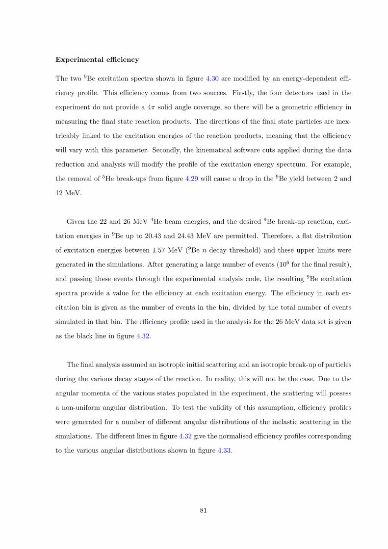
Experimental e�ciency

The two 9Be excitation spectra shown in figure 4.30 are modified by an energy-dependent e�-

ciency profile. This e�ciency comes from two sources. Firstly, the four detectors used in the

experiment do not provide a 4⇡ solid angle coverage, so there will be a geometric e�ciency in

measuring the final state reaction products. The directions of the final state particles are inex-

tricably linked to the excitation energies of the reaction products, meaning that the e�ciency

will vary with this parameter. Secondly, the kinematical software cuts applied during the data

reduction and analysis will modify the profile of the excitation energy spectrum. For example,

the removal of 5He break-ups from figure 4.29 will cause a drop in the 9Be yield between 2 and

12 MeV.

Given the 22 and 26 MeV 4He beam energies, and the desired 9Be break-up reaction, exci-

tation energies in 9Be up to 20.43 and 24.43 MeV are permitted. Therefore, a flat distribution

of excitation energies between 1.57 MeV (9Be n decay threshold) and these upper limits were

generated in the simulations. After generating a large number of events (106 for the final result),

and passing these events through the experimental analysis code, the resulting 9Be excitation

spectra provide a value for the e�ciency at each excitation energy. The e�ciency in each ex-

citation bin is given as the number of events in the bin, divided by the total number of events

simulated in that bin. The e�ciency profile used in the analysis for the 26 MeV data set is given

as the black line in figure 4.32.

The final analysis assumed an isotropic initial scattering and an isotropic break-up of particles

during the various decay stages of the reaction. In reality, this will not be the case. Due to the

angular momenta of the various states populated in the experiment, the scattering will possess

a non-uniform angular distribution. To test the validity of this assumption, e�ciency profiles

were generated for a number of di↵erent angular distributions of the inelastic scattering in the

simulations. The di↵erent lines in figure 4.32 give the normalised e�ciency profiles corresponding

to the various angular distributions shown in figure 4.33.

81

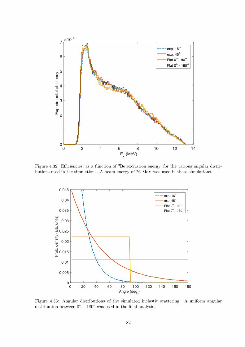
0 2 4 6 8 10 12 14Ex (MeV)

0

1

2

3

4

5

6

7

Expe

rimen

tal e

ffici

ency

�10-4

exp. 16o

exp. 45o

Flat 0o - 90o

Flat 0o - 180o

Figure 4.32: E�ciencies, as a function of 9Be excitation energy, for the various angular distri-butions used in the simulations. A beam energy of 26 MeV was used in these simulations.

0 20 40 60 80 100 120 140 160 180Angle (deg.)

0

0.005

0.01

0.015

0.02

0.025

0.03

0.035

0.04

0.045

Prob

. den

sity

(arb

. uni

ts)

exp. 16o

exp. 45o

Flat 0o - 90o

Flat 0o - 180o

Figure 4.33: Angular distributions of the simulated inelastic scattering. A uniform angulardistribution between 0� � 180� was used in the final analysis.

82

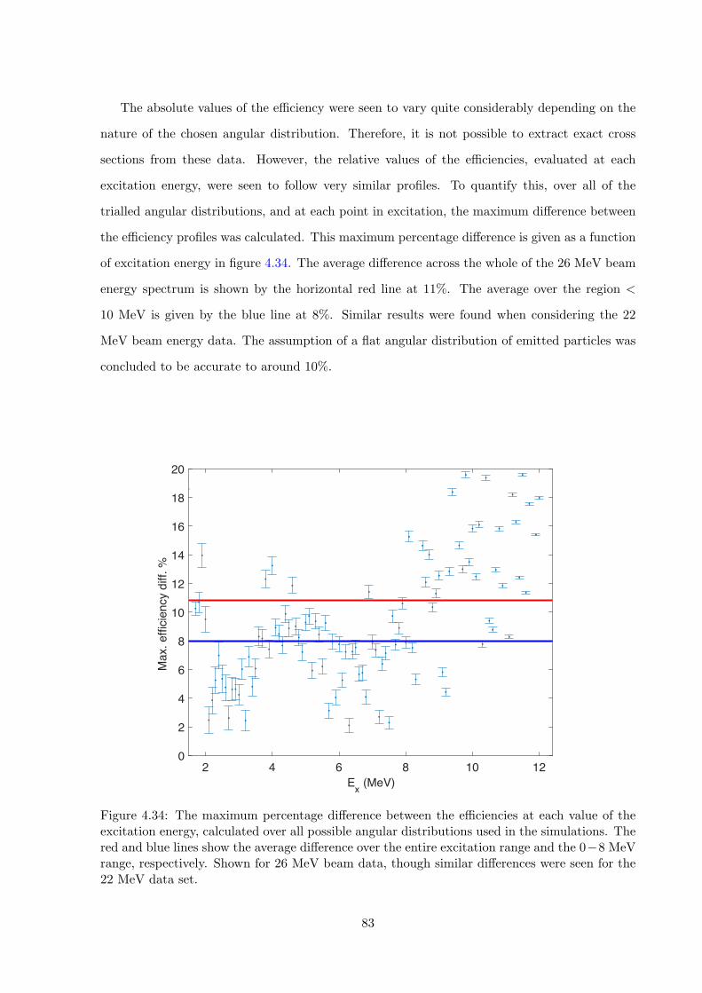
The absolute values of the e�ciency were seen to vary quite considerably depending on the

nature of the chosen angular distribution. Therefore, it is not possible to extract exact cross

sections from these data. However, the relative values of the e�ciencies, evaluated at each

excitation energy, were seen to follow very similar profiles. To quantify this, over all of the

trialled angular distributions, and at each point in excitation, the maximum di↵erence between

the e�ciency profiles was calculated. This maximum percentage di↵erence is given as a function

of excitation energy in figure 4.34. The average di↵erence across the whole of the 26 MeV beam

energy spectrum is shown by the horizontal red line at 11%. The average over the region <

10 MeV is given by the blue line at 8%. Similar results were found when considering the 22

MeV beam energy data. The assumption of a flat angular distribution of emitted particles was

concluded to be accurate to around 10%.

2 4 6 8 10 12Ex (MeV)

0

2

4

6

8

10

12

14

16

18

20

Max

. effi

cien

cy d

iff. %

Figure 4.34: The maximum percentage di↵erence between the e�ciencies at each value of theexcitation energy, calculated over all possible angular distributions used in the simulations. Thered and blue lines show the average di↵erence over the entire excitation range and the 0�8 MeVrange, respectively. Shown for 26 MeV beam data, though similar di↵erences were seen for the22 MeV data set.

83

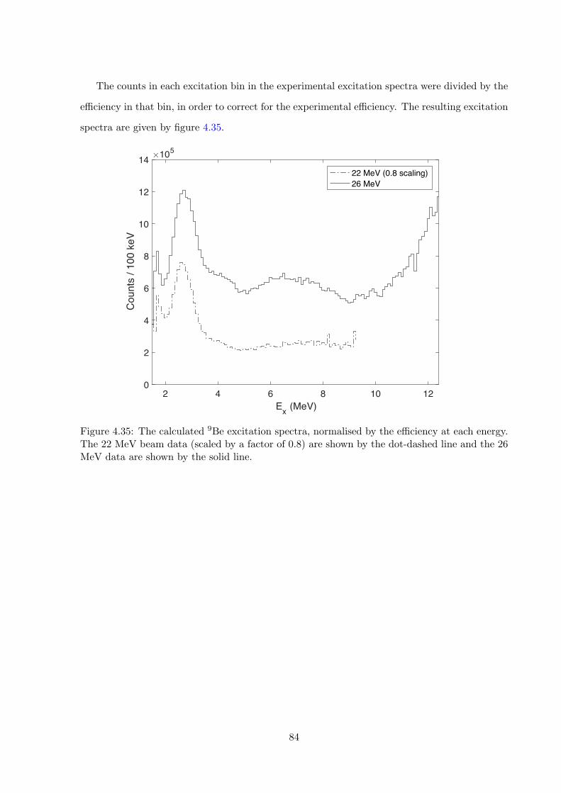
The counts in each excitation bin in the experimental excitation spectra were divided by the

e�ciency in that bin, in order to correct for the experimental e�ciency. The resulting excitation

spectra are given by figure 4.35.

2 4 6 8 10 12Ex (MeV)

0

2

4

6

8

10

12

14

Cou

nts

/ 100

keV

�105

22 MeV (0.8 scaling)26 MeV

Figure 4.35: The calculated 9Be excitation spectra, normalised by the e�ciency at each energy.The 22 MeV beam data (scaled by a factor of 0.8) are shown by the dot-dashed line and the 26MeV data are shown by the solid line.

84

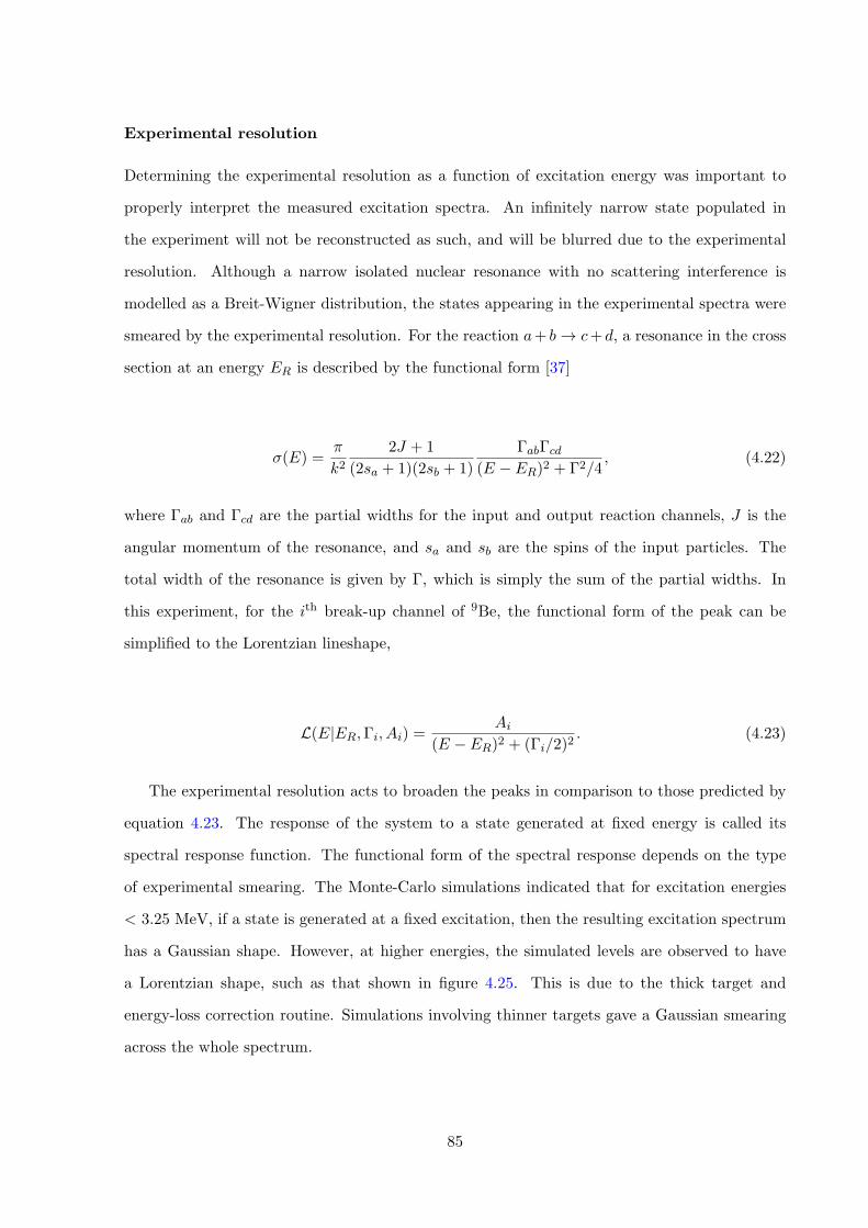
Experimental resolution

Determining the experimental resolution as a function of excitation energy was important to

properly interpret the measured excitation spectra. An infinitely narrow state populated in

the experiment will not be reconstructed as such, and will be blurred due to the experimental

resolution. Although a narrow isolated nuclear resonance with no scattering interference is

modelled as a Breit-Wigner distribution, the states appearing in the experimental spectra were

smeared by the experimental resolution. For the reaction a+ b ! c+d, a resonance in the cross

section at an energy ER is described by the functional form [37]

�(E) =⇡

k22J + 1

(2sa + 1)(2sb + 1)

�ab�cd(E � ER)2 + �2/4

, (4.22)

where �ab and �cd are the partial widths for the input and output reaction channels, J is the

angular momentum of the resonance, and sa and sb are the spins of the input particles. The

total width of the resonance is given by �, which is simply the sum of the partial widths. In

this experiment, for the ith break-up channel of 9Be, the functional form of the peak can be

simplified to the Lorentzian lineshape,

L(E|ER,�i, Ai) =Ai

(E � ER)2 + (�i/2)2. (4.23)

The experimental resolution acts to broaden the peaks in comparison to those predicted by

equation 4.23. The response of the system to a state generated at fixed energy is called its

spectral response function. The functional form of the spectral response depends on the type

of experimental smearing. The Monte-Carlo simulations indicated that for excitation energies

< 3.25 MeV, if a state is generated at a fixed excitation, then the resulting excitation spectrum

has a Gaussian shape. However, at higher energies, the simulated levels are observed to have

a Lorentzian shape, such as that shown in figure 4.25. This is due to the thick target and

energy-loss correction routine. Simulations involving thinner targets gave a Gaussian smearing

across the whole spectrum.

85

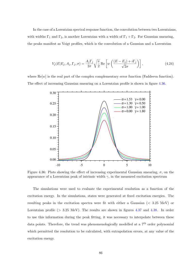
In the case of a Lorentzian spectral response function, the convolution between two Lorentzians,

with widths �1 and �2, is another Lorentzian with a width of �1 + �2. For Gaussian smearing,

the peaks manifest as Voigt profiles, which is the convolution of a Gaussian and a Lorentzian

Vj(E|Ej , Aj ,�j ,�) =Aj�j2�

r⇡

2Re

w

✓(E � Ej) + i�jp

2�

◆�, (4.24)

where Re[w] is the real part of the complex complementary error function (Faddeeva function).

The e↵ect of increasing Gaussian smearing on a Lorentzian profile is shown in figure 4.36.

Figure 4.36: Plots showing the e↵ect of increasing experimental Gaussian smearing, �, on theappearance of a Lorentzian peak of intrinsic width �, in the measured excitation spectrum

The simulations were used to evaluate the experimental resolution as a function of the

excitation energy. In the simulations, states were generated at fixed excitation energies. The

resulting peaks in the excitation spectra were fit with either a Gaussian (< 3.25 MeV) or

Lorentzian profile (> 3.25 MeV). The results are shown in figures 4.37 and 4.38. In order

to use this information during the peak fitting, it was necessary to interpolate between these

data points. Therefore, the trend was phenomenologically modelled at a 7th order polynomial

which permitted the resolution to be calculated, with extrapolation errors, at any value of the

excitation energy.

86

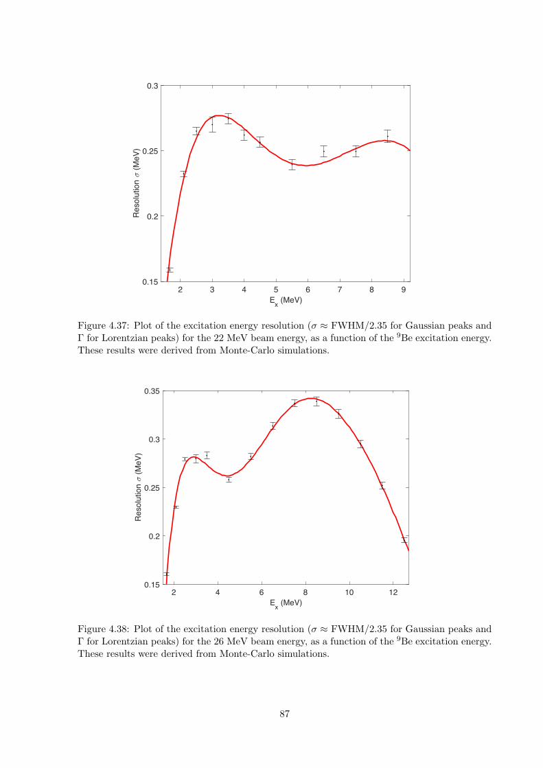
2 3 4 5 6 7 8 9Ex (MeV)

0.15

0.2

0.25

0.3

Res

olut

ion �

(MeV

)

Figure 4.37: Plot of the excitation energy resolution (� ⇡ FWHM/2.35 for Gaussian peaks and� for Lorentzian peaks) for the 22 MeV beam energy, as a function of the 9Be excitation energy.These results were derived from Monte-Carlo simulations.

2 4 6 8 10 12Ex (MeV)

0.15

0.2

0.25

0.3

0.35

Res

olut

ion �

(MeV

)

Figure 4.38: Plot of the excitation energy resolution (� ⇡ FWHM/2.35 for Gaussian peaks and� for Lorentzian peaks) for the 26 MeV beam energy, as a function of the 9Be excitation energy.These results were derived from Monte-Carlo simulations.

87

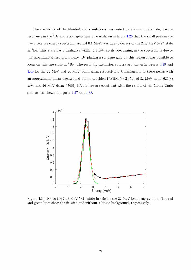
The credibility of the Monte-Carlo simulations was tested by examining a single, narrow

resonance in the 9Be excitation spectrum. It was shown in figure 4.26 that the small peak in the

↵�↵ relative energy spectrum, around 0.6 MeV, was due to decays of the 2.43 MeV 5/2� state

in 9Be. This state has a negligible width < 1 keV, so its broadening in the spectrum is due to

the experimental resolution alone. By placing a software gate on this region it was possible to

focus on this one state in 9Be. The resulting excitation spectra are shown in figures 4.39 and

4.40 for the 22 MeV and 26 MeV beam data, respectively. Gaussian fits to these peaks with

an approximate linear background profile provided FWHM (⇡ 2.35�) of 22 MeV data: 626(8)

keV, and 26 MeV data: 676(9) keV. These are consistent with the results of the Monte-Carlo

simulations shown in figures 4.37 and 4.38.

0 1 2 3 4 5 6 7Energy (MeV)

0

0.2

0.4

0.6

0.8

1

1.2

1.4

1.6

1.8

2

Cou

nts

/ 100

keV

�104

Figure 4.39: Fit to the 2.43 MeV 5/2� state in 9Be for the 22 MeV beam energy data. The redand green lines show the fit with and without a linear background, respectively.

88

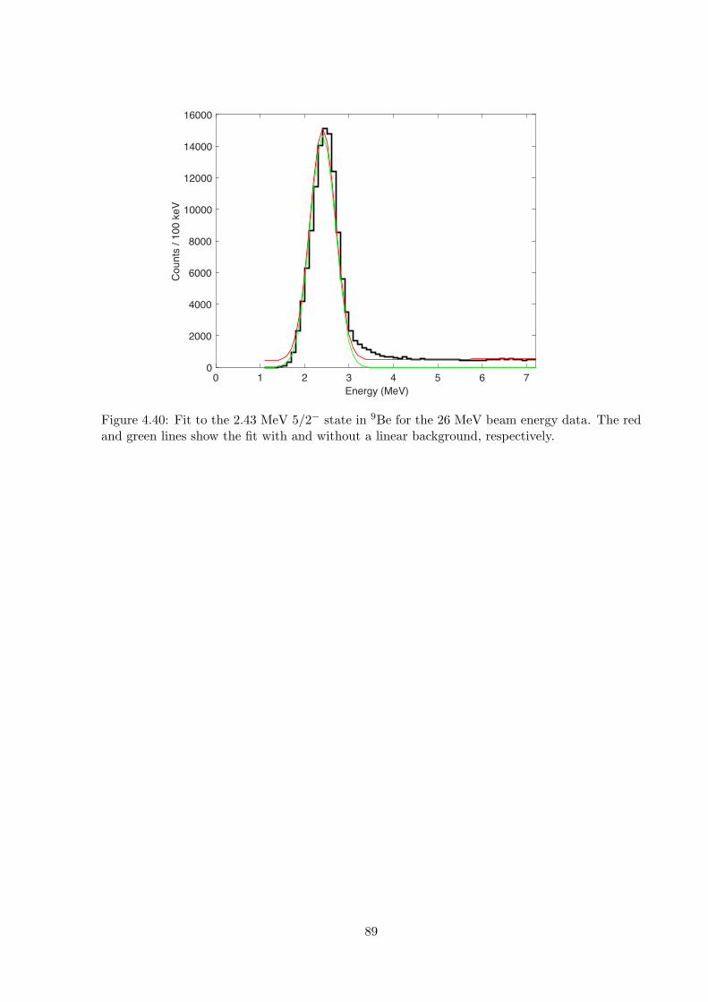
0 1 2 3 4 5 6 7Energy (MeV)

0

2000

4000

6000

8000

10000

12000

14000

16000

Cou

nts

/ 100

keV

Figure 4.40: Fit to the 2.43 MeV 5/2� state in 9Be for the 26 MeV beam energy data. The redand green lines show the fit with and without a linear background, respectively.

89

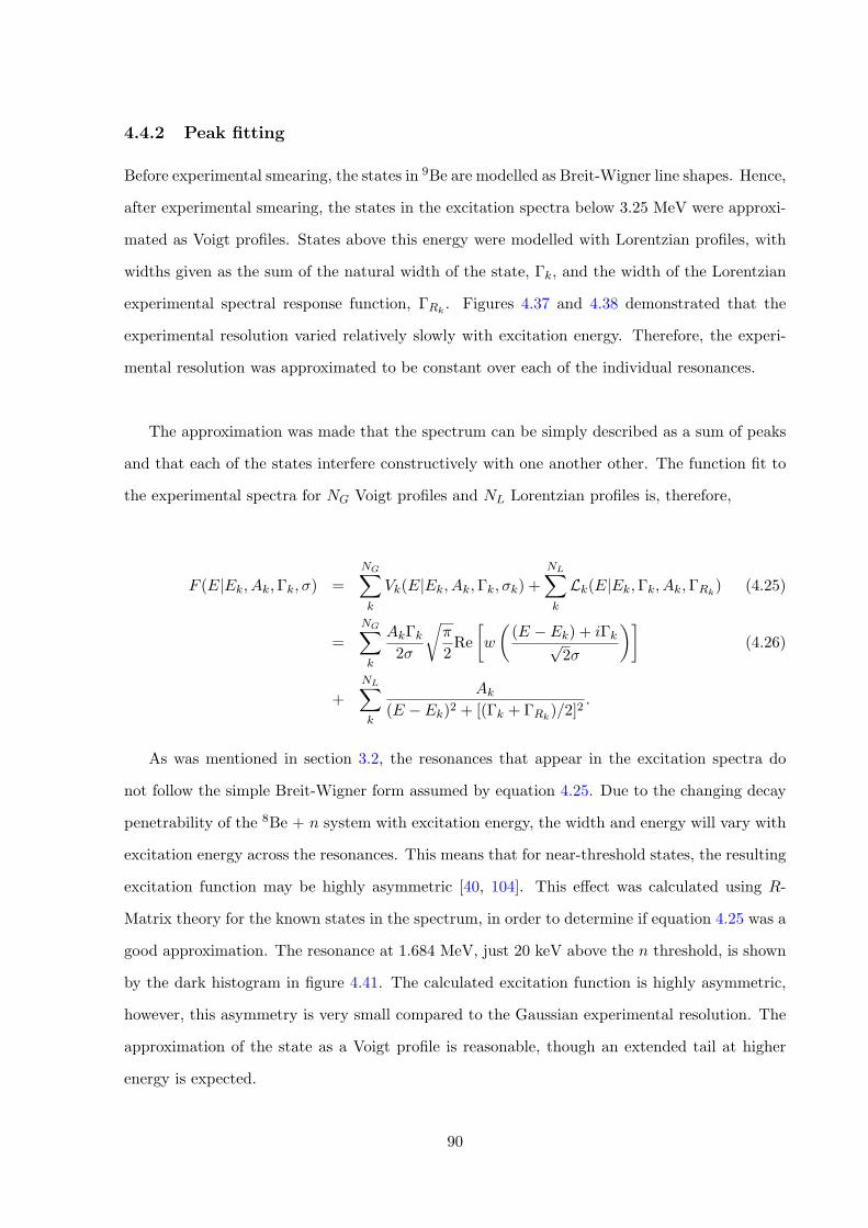
4.4.2 Peak fitting

Before experimental smearing, the states in 9Be are modelled as Breit-Wigner line shapes. Hence,

after experimental smearing, the states in the excitation spectra below 3.25 MeV were approxi-

mated as Voigt profiles. States above this energy were modelled with Lorentzian profiles, with

widths given as the sum of the natural width of the state, �k, and the width of the Lorentzian

experimental spectral response function, �Rk . Figures 4.37 and 4.38 demonstrated that the

experimental resolution varied relatively slowly with excitation energy. Therefore, the experi-

mental resolution was approximated to be constant over each of the individual resonances.

The approximation was made that the spectrum can be simply described as a sum of peaks

and that each of the states interfere constructively with one another other. The function fit to

the experimental spectra for NG Voigt profiles and NL Lorentzian profiles is, therefore,

F (E|Ek, Ak,�k,�) =NGX

k

Vk(E|Ek, Ak,�k,�k) +NLX

k

Lk(E|Ek,�k, Ak,�Rk) (4.25)

=NGX

k

Ak�k2�

r⇡

2Re

w

✓(E � Ek) + i�kp

2�

◆�(4.26)

+NLX

k

Ak

(E � Ek)2 + [(�k + �Rk)/2]2.

As was mentioned in section 3.2, the resonances that appear in the excitation spectra do

not follow the simple Breit-Wigner form assumed by equation 4.25. Due to the changing decay

penetrability of the 8Be + n system with excitation energy, the width and energy will vary with

excitation energy across the resonances. This means that for near-threshold states, the resulting

excitation function may be highly asymmetric [40, 104]. This e↵ect was calculated using R-

Matrix theory for the known states in the spectrum, in order to determine if equation 4.25 was a

good approximation. The resonance at 1.684 MeV, just 20 keV above the n threshold, is shown

by the dark histogram in figure 4.41. The calculated excitation function is highly asymmetric,

however, this asymmetry is very small compared to the Gaussian experimental resolution. The

approximation of the state as a Voigt profile is reasonable, though an extended tail at higher

energy is expected.

90

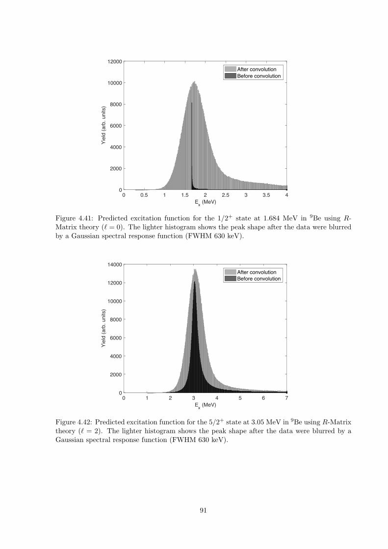
0 0.5 1 1.5 2 2.5 3 3.5 4Ex (MeV)

0

2000

4000

6000

8000

10000

12000

Yiel

d (a

rb. u

nits

)

After convolutionBefore convolution

Figure 4.41: Predicted excitation function for the 1/2+ state at 1.684 MeV in 9Be using R-Matrix theory (` = 0). The lighter histogram shows the peak shape after the data were blurredby a Gaussian spectral response function (FWHM 630 keV).

0 1 2 3 4 5 6 7Ex (MeV)

0

2000

4000

6000

8000

10000

12000

14000

Yiel

d (a

rb. u

nits

)

After convolutionBefore convolution

Figure 4.42: Predicted excitation function for the 5/2+ state at 3.05 MeV in 9Be using R-Matrixtheory (` = 2). The lighter histogram shows the peak shape after the data were blurred by aGaussian spectral response function (FWHM 630 keV).

91

The 5/2+ state at 3.05 MeV was also generated using R-matrix theory and was seen to be

slightly asymmetric in figure 4.42. Again, the Gaussian experimental smearing dominates the

asymmetry. The R-Matrix calculations were performed using an unpublished code, and verified

using the AZURE2 code [51, 105]. It was concluded that, given the experimental resolution, the

form of equation 4.25 was a reasonable function to fit to the experimental data.

The data were fit using the Tracey Peaker v 1.0 �2 minimisation program (MATLAB 2012a)

[106]. Initially, the known states in 9Be [52] were fit to the excitation spectra and the results

are shown by figures 4.43 and 4.44.

2 3 4 5 6 7 8 9Ex (MeV)

0

2

4

6

8

10

12

Cou

nts

/ 100

keV

�105

22 MeV Data Least Squares Fit Quadratic background Individual States

2 3 4 5 6 7 8 9Ex (MeV)

-1

-0.5

0

0.5

1

Res

idua

ls /

100

keV

�105

χ2/DoF=4.81

Figure 4.43: Fit of the known levels in 9Be to the 22 MeV beam energy excitation spectrum.The lower panel shows the fit residuals, indicating an extra feature in the 4 MeV region.

92

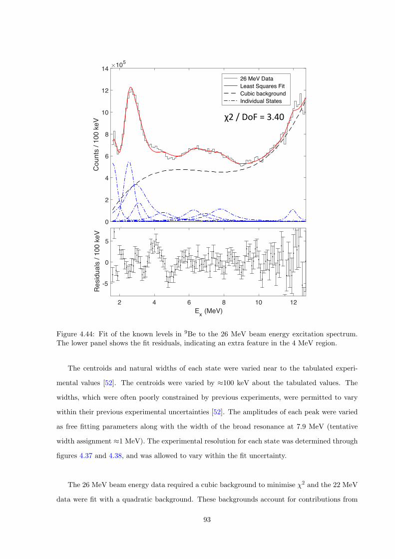
2 4 6 8 10 12Ex (MeV)

0

2

4

6

8

10

12

14

Cou

nts

/ 100

keV

�105

26 MeV Data Least Squares Fit Cubic background Individual States

2 4 6 8 10 12Ex (MeV)

-5

0

5

Res

idua

ls /

100

keV

�104

χ2/DoF=3.40

Figure 4.44: Fit of the known levels in 9Be to the 26 MeV beam energy excitation spectrum.The lower panel shows the fit residuals, indicating an extra feature in the 4 MeV region.

The centroids and natural widths of each state were varied near to the tabulated experi-

mental values [52]. The centroids were varied by ⇡100 keV about the tabulated values. The

widths, which were often poorly constrained by previous experiments, were permitted to vary

within their previous experimental uncertainties [52]. The amplitudes of each peak were varied

as free fitting parameters along with the width of the broad resonance at 7.9 MeV (tentative

width assignment ⇡1 MeV). The experimental resolution for each state was determined through

figures 4.37 and 4.38, and was allowed to vary within the fit uncertainty.

The 26 MeV beam energy data required a cubic background to minimise �2 and the 22 MeV

data were fit with a quadratic background. These backgrounds account for contributions from

93

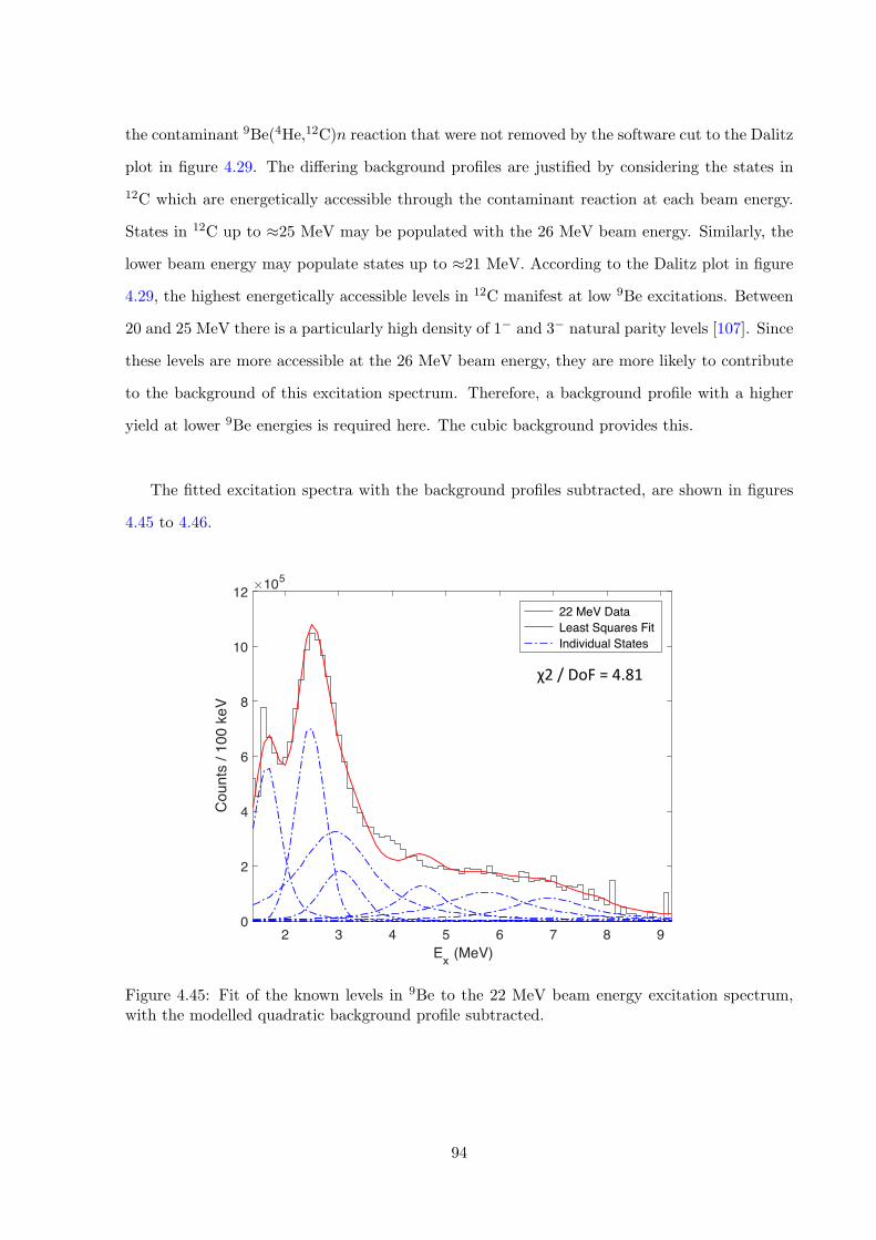
the contaminant 9Be(4He,12C)n reaction that were not removed by the software cut to the Dalitz

plot in figure 4.29. The di↵ering background profiles are justified by considering the states in

12C which are energetically accessible through the contaminant reaction at each beam energy.

States in 12C up to ⇡25 MeV may be populated with the 26 MeV beam energy. Similarly, the

lower beam energy may populate states up to ⇡21 MeV. According to the Dalitz plot in figure

4.29, the highest energetically accessible levels in 12C manifest at low 9Be excitations. Between

20 and 25 MeV there is a particularly high density of 1� and 3� natural parity levels [107]. Since

these levels are more accessible at the 26 MeV beam energy, they are more likely to contribute

to the background of this excitation spectrum. Therefore, a background profile with a higher

yield at lower 9Be energies is required here. The cubic background provides this.

The fitted excitation spectra with the background profiles subtracted, are shown in figures

4.45 to 4.46.

2 3 4 5 6 7 8 9Ex (MeV)

0

2

4

6

8

10

12

Cou

nts

/ 100

keV

�105

22 MeV Data Least Squares Fit Individual States

χ2/DoF=4.81

Figure 4.45: Fit of the known levels in 9Be to the 22 MeV beam energy excitation spectrum,with the modelled quadratic background profile subtracted.

94

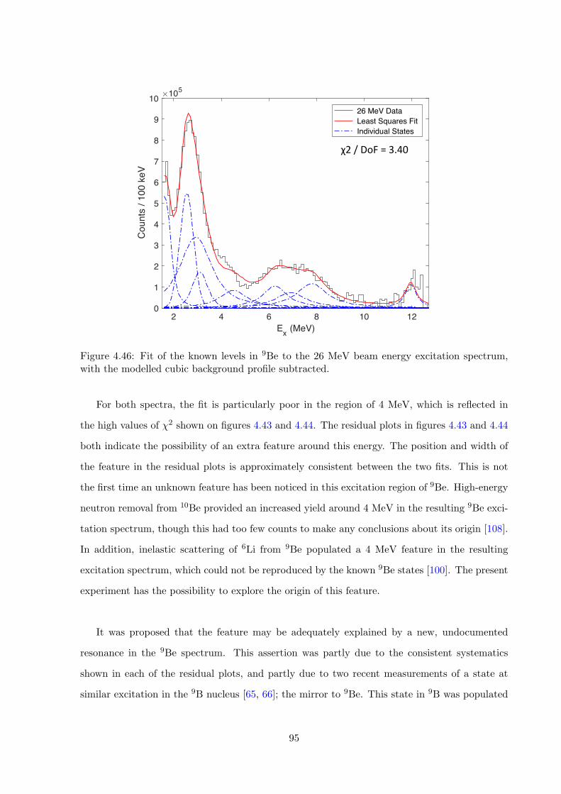
2 4 6 8 10 12Ex (MeV)

0

1

2

3

4

5

6

7

8

9

10

Cou

nts

/ 100

keV

�105

26 MeV Data Least Squares Fit Individual States

χ2/DoF=3.40

Figure 4.46: Fit of the known levels in 9Be to the 26 MeV beam energy excitation spectrum,with the modelled cubic background profile subtracted.

For both spectra, the fit is particularly poor in the region of 4 MeV, which is reflected in

the high values of �2 shown on figures 4.43 and 4.44. The residual plots in figures 4.43 and 4.44

both indicate the possibility of an extra feature around this energy. The position and width of

the feature in the residual plots is approximately consistent between the two fits. This is not

the first time an unknown feature has been noticed in this excitation region of 9Be. High-energy

neutron removal from 10Be provided an increased yield around 4 MeV in the resulting 9Be exci-

tation spectrum, though this had too few counts to make any conclusions about its origin [108].

In addition, inelastic scattering of 6Li from 9Be populated a 4 MeV feature in the resulting

excitation spectrum, which could not be reproduced by the known 9Be states [100]. The present

experiment has the possibility to explore the origin of this feature.

It was proposed that the feature may be adequately explained by a new, undocumented

resonance in the 9Be spectrum. This assertion was partly due to the consistent systematics

shown in each of the residual plots, and partly due to two recent measurements of a state at

similar excitation in the 9B nucleus [65, 66]; the mirror to 9Be. This state in 9B was populated

95

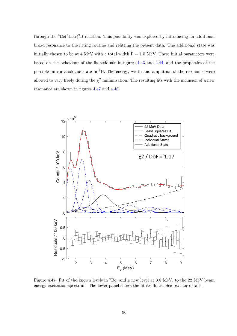
through the 9Be(3He,t)9B reaction. This possibility was explored by introducing an additional

broad resonance to the fitting routine and refitting the present data. The additional state was

initially chosen to be at 4 MeV with a total width � = 1.5 MeV. These initial parameters were

based on the behaviour of the fit residuals in figures 4.43 and 4.44, and the properties of the

possible mirror analogue state in 9B. The energy, width and amplitude of the resonance were

allowed to vary freely during the �2 minimisation. The resulting fits with the inclusion of a new

resonance are shown in figures 4.47 and 4.48.

2 3 4 5 6 7 8 9Ex (MeV)

0

2

4

6

8

10

12

Cou

nts

/ 100

keV

�105

22 MeV Data Least Squares Fit Quadratic background Individual States

2 3 4 5 6 7 8 9Ex (MeV)

-1

-0.5

0

0.5

1

Res

idua

ls /

100

keV

�105

χ2/DoF=1.17

Additional State

Figure 4.47: Fit of the known levels in 9Be, and a new level at 3.8 MeV, to the 22 MeV beamenergy excitation spectrum. The lower panel shows the fit residuals. See text for details.

96

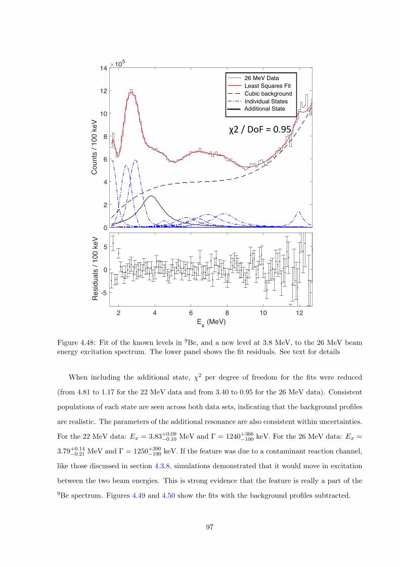
2 3 4 5 6 7 8 9Ex (MeV)

0

2

4

6

8

10

12

Cou

nts

/ 100

keV

�105

22 MeV Data Least Squares Fit Quadratic background Individual States

2 4 6 8 10 12Ex (MeV)

0

2

4

6

8

10

12

14

Cou

nts

/ 100

keV

�105

26 MeV Data Least Squares Fit Cubic background Individual States

2 4 6 8 10 12Ex (MeV)

-5

0

5

Res

idua

ls /

100

keV

�104

χ2/DoF=0.95

Additional State

Figure 4.48: Fit of the known levels in 9Be, and a new level at 3.8 MeV, to the 26 MeV beamenergy excitation spectrum. The lower panel shows the fit residuals. See text for details

When including the additional state, �2 per degree of freedom for the fits were reduced

(from 4.81 to 1.17 for the 22 MeV data and from 3.40 to 0.95 for the 26 MeV data). Consistent

populations of each state are seen across both data sets, indicating that the background profiles

are realistic. The parameters of the additional resonance are also consistent within uncertainties.

For the 22 MeV data: Ex = 3.83+0.09�0.10 MeV and � = 1240+366

�100 keV. For the 26 MeV data: Ex =

3.79+0.14�0.21 MeV and � = 1250+390

�190 keV. If the feature was due to a contaminant reaction channel,

like those discussed in section 4.3.8, simulations demonstrated that it would move in excitation

between the two beam energies. This is strong evidence that the feature is really a part of the

9Be spectrum. Figures 4.49 and 4.50 show the fits with the background profiles subtracted.

97

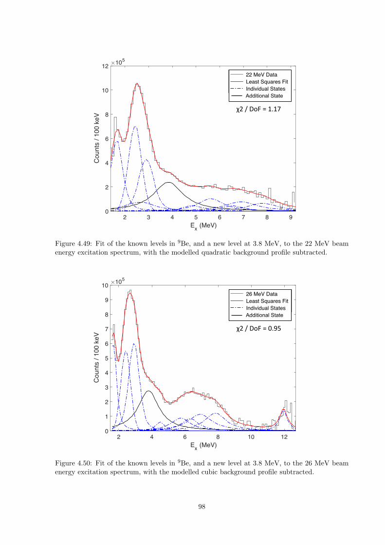
2 3 4 5 6 7 8 9Ex (MeV)

0

2

4

6

8

10

12

Cou

nts

/ 100

keV

�105

22 MeV Data Least Squares Fit Individual States

χ2/DoF=1.17

Additional State

Figure 4.49: Fit of the known levels in 9Be, and a new level at 3.8 MeV, to the 22 MeV beamenergy excitation spectrum, with the modelled quadratic background profile subtracted.

2 4 6 8 10 12Ex (MeV)

0

1

2

3

4

5

6

7

8

9

10

Cou

nts

/ 100

keV

�105

26 MeV Data Least Squares Fit Individual States

χ2/DoF=0.95

Additional State

Figure 4.50: Fit of the known levels in 9Be, and a new level at 3.8 MeV, to the 26 MeV beamenergy excitation spectrum, with the modelled cubic background profile subtracted.

98

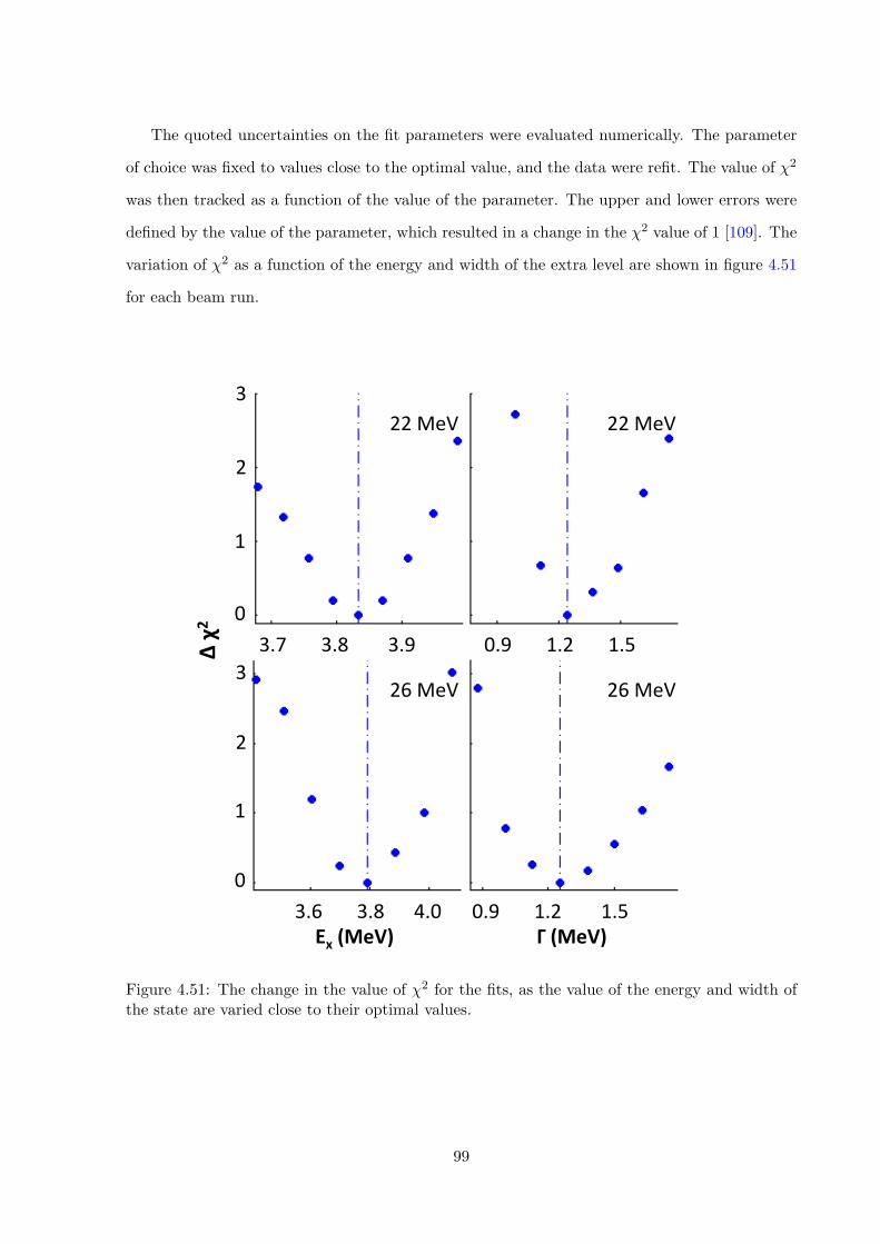
The quoted uncertainties on the fit parameters were evaluated numerically. The parameter

of choice was fixed to values close to the optimal value, and the data were refit. The value of �2

was then tracked as a function of the value of the parameter. The upper and lower errors were

defined by the value of the parameter, which resulted in a change in the �2 value of 1 [109]. The

variation of �2 as a function of the energy and width of the extra level are shown in figure 4.51

for each beam run.

Δχ2

Ex(MeV) Γ(MeV)3.63.84.0 0.91.21.5

0.91.21.53.73.83.9

0

1

2

3

0

1

2

3

26MeV 26MeV

22MeV 22MeV

Figure 4.51: The change in the value of �2 for the fits, as the value of the energy and width ofthe state are varied close to their optimal values.

99

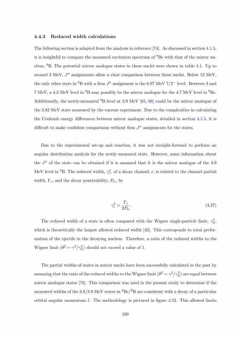
4.4.3 Reduced width calculations

The following section is adapted from the analysis in reference [74]. As discussed in section 4.1.5,

it is insightful to compare the measured excitation spectrum of 9Be with that of the mirror nu-

cleus, 9B. The potential mirror analogue states in these nuclei were shown in table 4.1. Up to

around 3 MeV, J⇡ assignments allow a clear comparison between these nuclei. Below 12 MeV,

the only other state in 9B with a firm J⇡ assignment is the 6.97 MeV 7/2� level. Between 3 and

7 MeV, a 4.3 MeV level in 9B may possibly be the mirror analogue for the 4.7 MeV level in 9Be.

Additionally, the newly-measured 9B level at 3.9 MeV [65, 66] could be the mirror analogue of

the 3.82 MeV state measured by the current experiment. Due to the complexities in calculating

the Coulomb energy di↵erences between mirror analogue states, detailed in section 4.1.5, it is

di�cult to make confident comparisons without firm J⇡ assignments for the states.

Due to the experimental set-up and reaction, it was not straight-forward to perform an

angular distribution analysis for the newly-measured state. However, some information about

the J⇡ of the state can be obtained if it is assumed that it is the mirror analogue of the 3.9

MeV level in 9B. The reduced width, �2c , of a decay channel, c, is related to the channel partial

width, �c, and the decay penetrability, P`c, by

�2c =�c2P`c

. (4.27)

The reduced width of a state is often compared with the Wigner single-particle limit, �2w,

which is theoretically the largest allowed reduced width [42]. This corresponds to total prefor-

mation of the ejectile in the decaying nucleus. Therefore, a ratio of the reduced widths to the

Wigner limit (✓2 = �2/�2w) should not exceed a value of 1.

The partial widths of states in mirror nuclei have been successfully calculated in the past by

assuming that the ratio of the reduced widths to the Wigner limit (✓2 = �2/�2w) are equal between

mirror analogue states [78]. This comparison was used in the present study to determine if the

measured widths of the 3.8/3.9 MeV states in 9Be/9B are consistent with a decay of a particular

orbital angular momentum `. The methodology is pictured in figure 4.52. This allowed limits

100

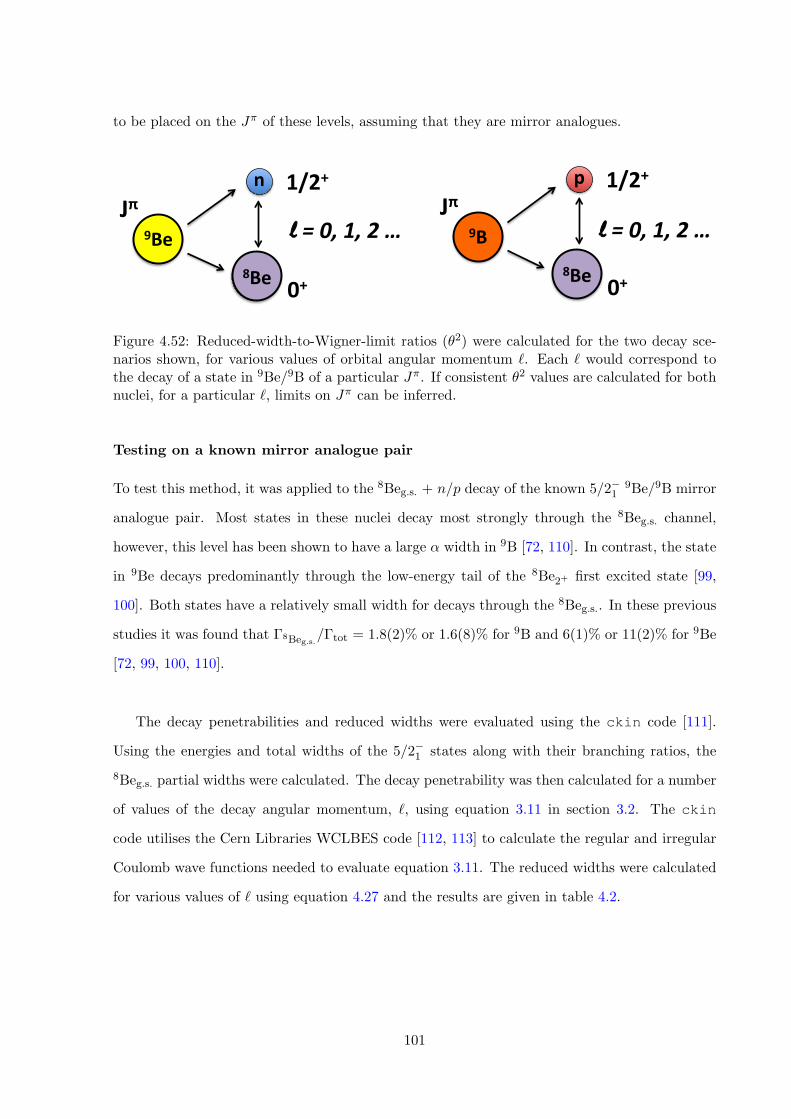
to be placed on the J⇡ of these levels, assuming that they are mirror analogues.

9Be

8Be

nJπ

0+

1/2+

9B

8Be

pJπ

0+

1/2+

l=0,1,2… l=0,1,2…

Figure 4.52: Reduced-width-to-Wigner-limit ratios (✓2) were calculated for the two decay sce-narios shown, for various values of orbital angular momentum `. Each ` would correspond tothe decay of a state in 9Be/9B of a particular J⇡. If consistent ✓2 values are calculated for bothnuclei, for a particular `, limits on J⇡ can be inferred.

Testing on a known mirror analogue pair

To test this method, it was applied to the 8Beg.s. + n/p decay of the known 5/2�19Be/9B mirror

analogue pair. Most states in these nuclei decay most strongly through the 8Beg.s. channel,

however, this level has been shown to have a large ↵ width in 9B [72, 110]. In contrast, the state

in 9Be decays predominantly through the low-energy tail of the 8Be2+ first excited state [99,

100]. Both states have a relatively small width for decays through the 8Beg.s.. In these previous

studies it was found that �8Beg.s.

/�tot = 1.8(2)% or 1.6(8)% for 9B and 6(1)% or 11(2)% for 9Be

[72, 99, 100, 110].

The decay penetrabilities and reduced widths were evaluated using the ckin code [111].

Using the energies and total widths of the 5/2�1 states along with their branching ratios, the

8Beg.s. partial widths were calculated. The decay penetrability was then calculated for a number

of values of the decay angular momentum, `, using equation 3.11 in section 3.2. The ckin

code utilises the Cern Libraries WCLBES code [112, 113] to calculate the regular and irregular

Coulomb wave functions needed to evaluate equation 3.11. The reduced widths were calculated

for various values of ` using equation 4.27 and the results are given in table 4.2.

101

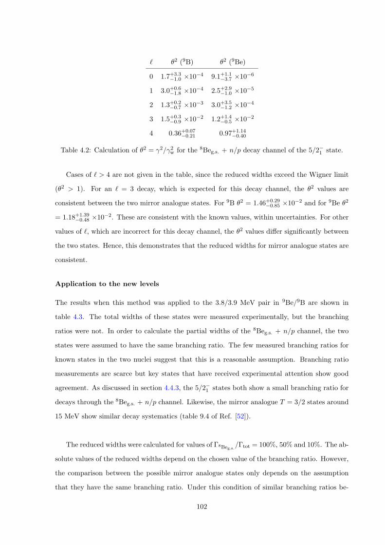
` ✓2 (9B) ✓2 (9Be)

0 1.7+3.3�1.0 ⇥10�4 9.1+1.1

�3.7 ⇥10�6

1 3.0+0.6�1.8 ⇥10�4 2.5+2.9

�1.0 ⇥10�5

2 1.3+0.2�0.7 ⇥10�3 3.0+3.5

�1.2 ⇥10�4

3 1.5+0.3�0.9 ⇥10�2 1.2+1.4

�0.5 ⇥10�2

4 0.36+0.07�0.21 0.97+1.14

�0.40

Table 4.2: Calculation of ✓2 = �2/�2w for the 8Beg.s. + n/p decay channel of the 5/2�1 state.

Cases of ` > 4 are not given in the table, since the reduced widths exceed the Wigner limit

(✓2 > 1). For an ` = 3 decay, which is expected for this decay channel, the ✓2 values are

consistent between the two mirror analogue states. For 9B ✓2 = 1.46+0.29�0.85 ⇥10�2 and for 9Be ✓2

= 1.18+1.39�0.48 ⇥10�2. These are consistent with the known values, within uncertainties. For other

values of `, which are incorrect for this decay channel, the ✓2 values di↵er significantly between

the two states. Hence, this demonstrates that the reduced widths for mirror analogue states are

consistent.

Application to the new levels

The results when this method was applied to the 3.8/3.9 MeV pair in 9Be/9B are shown in

table 4.3. The total widths of these states were measured experimentally, but the branching

ratios were not. In order to calculate the partial widths of the 8Beg.s. + n/p channel, the two

states were assumed to have the same branching ratio. The few measured branching ratios for

known states in the two nuclei suggest that this is a reasonable assumption. Branching ratio

measurements are scarce but key states that have received experimental attention show good

agreement. As discussed in section 4.4.3, the 5/2�1 states both show a small branching ratio for

decays through the 8Beg.s. + n/p channel. Likewise, the mirror analogue T = 3/2 states around

15 MeV show similar decay systematics (table 9.4 of Ref. [52]).

The reduced widths were calculated for values of �8Beg.s.

/�tot = 100%, 50% and 10%. The ab-

solute values of the reduced widths depend on the chosen value of the branching ratio. However,

the comparison between the possible mirror analogue states only depends on the assumption

that they have the same branching ratio. Under this condition of similar branching ratios be-

102

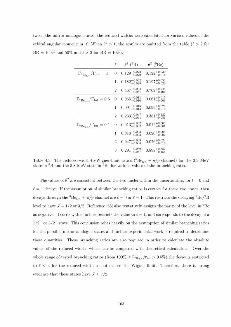
tween the mirror analogue states, the reduced widths were calculated for various values of the

orbital angular momentum, `. When ✓2 > 1, the results are omitted from the table (` > 2 for

BR = 100% and 50% and ` > 3 for BR = 10%).

` ✓2 (9B) ✓2 (9Be)

�8Beg.s.

/�tot = 1 0 0.129+0.022�0.020 0.122+0.030

�0.011

1 0.182+0.032�0.029 0.197+0.052

�0.020

2 0.467+0.094�0.081 0.762+0.244

�0.101

�8Beg.s.

/�tot = 0.5 0 0.065+0.011�0.010 0.061+0.015

�0.006

1 0.091+0.016�0.014 0.099+0.026

�0.010

2 0.233+0.047�0.041 0.381+0.122

�0.051

�8Beg.s.

/�tot = 0.1 0 0.013+0.002�0.002 0.012+0.003

�0.001

1 0.018+0.003�0.003 0.020+0.005

�0.002

2 0.047+0.009�0.008 0.076+0.024

�0.010

3 0.291+0.069�0.057 0.898+0.352

�0.155

Table 4.3: The reduced-width-to-Wigner-limit ratios (8Beg.s. + n/p channel) for the 3.9 MeVstate in 9B and the 3.8 MeV state in 9Be for various values of the branching ratio.

The values of ✓2 are consistent between the two nuclei within the uncertainties, for ` = 0 and

` = 1 decays. If the assumption of similar branching ratios is correct for these two states, then

decays through the 8Beg.s. + n/p channel are ` = 0 or ` = 1. This restricts the decaying 9Be/9B

level to have J = 1/2 or 3/2. Reference [65] also tentatively assigns the parity of the level in 9Be

as negative. If correct, this further restricts the value to ` = 1, and corresponds to the decay of a

1/2� or 3/2� state. This conclusion relies heavily on the assumption of similar branching ratios

for the possible mirror analogue states and further experimental work is required to determine

these quantities. These branching ratios are also required in order to calculate the absolute

values of the reduced widths which can be compared with theoretical calculations. Over the

whole range of tested branching ratios (from 100% � �8Beg.s./�tot

> 0.5%) the decay is restricted

to ` < 4 for the reduced width to not exceed the Wigner limit. Therefore, there is strong

evidence that these states have J 7/2.

103

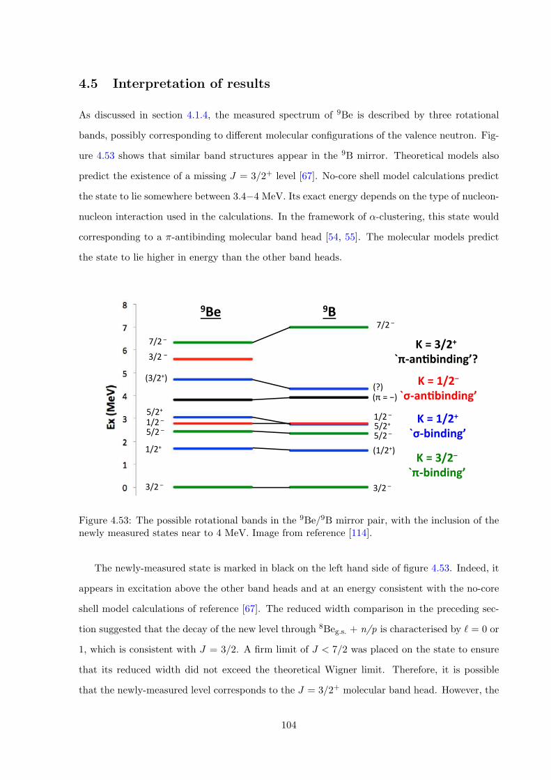
4.5 Interpretation of results

As discussed in section 4.1.4, the measured spectrum of 9Be is described by three rotational

bands, possibly corresponding to di↵erent molecular configurations of the valence neutron. Fig-

ure 4.53 shows that similar band structures appear in the 9B mirror. Theoretical models also

predict the existence of a missing J = 3/2+ level [67]. No-core shell model calculations predict

the state to lie somewhere between 3.4�4 MeV. Its exact energy depends on the type of nucleon-

nucleon interaction used in the calculations. In the framework of ↵-clustering, this state would

corresponding to a ⇡-antibinding molecular band head [54, 55]. The molecular models predict

the state to lie higher in energy than the other band heads.

K=3/2−`π-binding’

K=1/2+`σ-binding’

K=1/2−`σ-an5binding’

3/2–

5/2–

1/2+

5/2+

(3/2+)

1/2–

3/2–

3/2–

5/2–

(1/2+)

5/2+

(?)

1/2–

7/2–7/2–

(π=−)

9Be 9B

K=3/2+`π-an5binding’?

Figure 4.53: The possible rotational bands in the 9Be/9B mirror pair, with the inclusion of thenewly measured states near to 4 MeV. Image from reference [114].

The newly-measured state is marked in black on the left hand side of figure 4.53. Indeed, it

appears in excitation above the other band heads and at an energy consistent with the no-core

shell model calculations of reference [67]. The reduced width comparison in the preceding sec-

tion suggested that the decay of the new level through 8Beg.s. + n/p is characterised by ` = 0 or

1, which is consistent with J = 3/2. A firm limit of J < 7/2 was placed on the state to ensure

that its reduced width did not exceed the theoretical Wigner limit. Therefore, it is possible

that the newly-measured level corresponds to the J = 3/2+ molecular band head. However, the

104

proposed mirror analogue state in 9B has a tentative negative parity assignment, which does

not support this claim.

The reduced width analysis made the clear assumption that the levels in 9Be and 9B were

mirror analogue states. This assumption was based on their close proximity in energy alone, since

no reliable J⇡ assignments exist for these levels. This assumption is not unreasonable given the

low density of unassigned levels in this region and due to the fact that Coulomb energy di↵erences

are typically around 100 keV [73]. However, the origins of mirror energy di↵erences are quite

complicated, and it is possible that this pairing is incorrect. Assuming that the newly-measured

3.8 MeV level in 9Be and the 3.9 MeV level in 9B are mirror analogue states, insights into their

structure could be learned from the di↵erence in their excitation energies with respect to each of

the ground states. However, to make a quantitative comparison with the precise magnitude of

this shift and the structure described by the underlying wave functions, more theoretical input

is needed.

105

4.6 Outlook

Given the previous discussion, it is clear that measurements of the branching ratios for the pro-

posed 3.8/3.9 MeV mirror pair are required to add credence to the proposal that they correspond

to the ⇡-antibinding molecular band heads. The analysis currently relies on the assumption of

similar branching ratios between the two states, which may not be true. The ambiguity sur-

rounding the origin of the three final state ↵-particles in this experiment meant that only the

8Beg.s. + n/p channel could be examined. Selecting events where a pair of ↵-particles origi-

nated from the decay of 8Be cleanly tagged the third ↵-particle as the scattered beam. Using

a di↵erent beam such as 3He in conjunction with particle identification capabilities would in

principle make it clear which final-state charged particle is the scattered beam, and which result

from the 9Be break-up. The �8Beg.s.

/�tot branching ratio could then be evaluated. Measuring

the branching ratios for other decay channels would also be insightful. However, as references

[100] and [99] note, the 8Be2+ and 5Heg.s. channels have strongly overlapping signatures for low

energy states in 9Be, which hinders such an evaluation.

Another promising avenue would be to examine the excited states of 9Be populated through

a reaction other than direct inelastic scattering. Reference [115] examined states in 16O through

the 13C(4He,16O)n reaction. As part of this experiment, there is evidence for the 13C(4He,9Be)2↵

reaction as demonstrated by the 9Be excitation spectrum shown by figure 4.54. This can cor-

respond to inelastic scattering from 13C, populating excited states in this nucleus. These then

↵-decay, populating states in 9Be. By examining the excitation spectrum of 9Be resulting from

decays of states of particular J⇡ in 13C, and noting the relative intensities of the 9Be states

populated, the angular momenta of the states may be inferred due to the di↵erent centrifugal

barriers. For example, a 5/2� state in 13C will more readily decay to a 5/2� state in 9Be since

there is no centrifugal barrier. Decays to a 1/2+ state in 9Be would be suppressed due to the

additional angular momentum barrier. If the 3.8 MeV state in 9Be was recorded during this

experiment, more strict limits on its J⇡ may be obtained. The data from reference [115] have

been obtained and the analysis is ongoing.

106

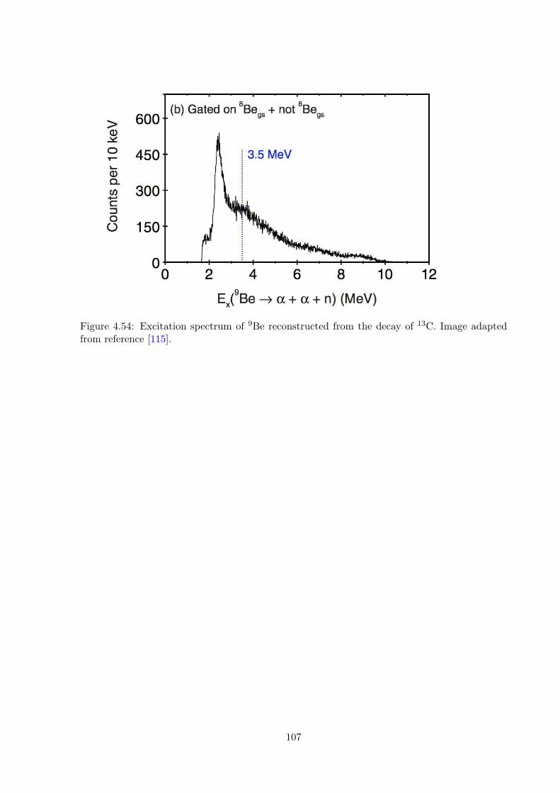
Figure 4.54: Excitation spectrum of 9Be reconstructed from the decay of 13C. Image adaptedfrom reference [115].

107

Chapter 5

Investigating the 3↵ break-up modes

of the 12C Hoyle state

It’snotyou,it’sme…

109

Chapter Abstract

The Hoyle state in 12C is a crucial resonance in nuclear astrophysics since it enhances stellar

helium burning through the triple-↵ process by over seven orders of magnitude. It is also in-

teresting from a nuclear structure perspective, since the dominant degrees of freedom of this

nucleus are those of ↵-particle clusters rather than individual nucleons. With this in mind, the

Hoyle state may possess a number of interesting intrinsic structures, corresponding to di↵erent

geometric configurations of its constituent ↵-particles. Indeed, theoretical calculations predict a

myriad of possibilities, which are often in disagreement with one another. Due to challenges in

experimentally confirming the structures of unbound nuclear states, insights into the structure of

the Hoyle state have been based on indirect evidence. Recently there have been a number of ex-

periments dedicated to measuring the rare direct decay of the Hoyle state into three ↵-particles,

since this observable could be a direct and sensitive probe of its 3↵ structure. However, previous

experiments have not been sensitive enough to measure this decay channel, which is severely

hindered by the available phase space. This chapter presents a high-precision measurement of

the 3↵ decay of the Hoyle state using the 12C(↵,↵)3↵ inelastic scattering reaction at 40 MeV

beam energy. The reaction products were measured using a bespoke array of double-sided sil-

icon strip detectors and the experimental data were compared to Monte-Carlo simulations of

sequential and direct decay mechanisms. No direct decays were observed, but an upper limit for

the direct decay branch of 0.047% was obtained � almost one order of magnitude lower than

previous experimental e↵orts. This value is lower than a number of theoretical estimates and

opens new intriguing questions about the structure of this state.

This work has been published in the following article. Some figures and text blocks from this

publication are used in the following chapter.

R. Smith, Tz. Kokalova, et al. New Measurement of the Direct 3↵ Decay from the 12C Hoyle

State, Phys. Rev. Lett. 119 (2017).

110

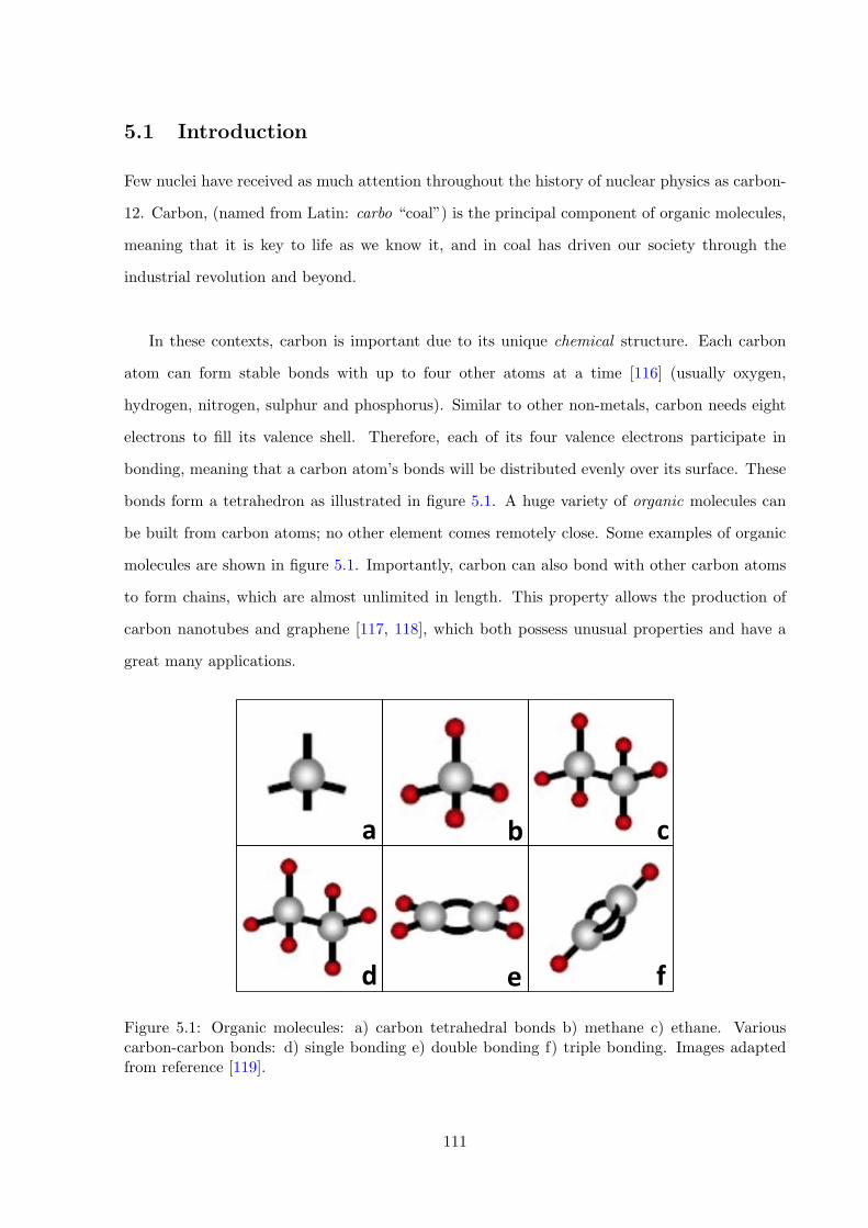
5.1 Introduction

Few nuclei have received as much attention throughout the history of nuclear physics as carbon-

12. Carbon, (named from Latin: carbo “coal”) is the principal component of organic molecules,

meaning that it is key to life as we know it, and in coal has driven our society through the

industrial revolution and beyond.

In these contexts, carbon is important due to its unique chemical structure. Each carbon

atom can form stable bonds with up to four other atoms at a time [116] (usually oxygen,

hydrogen, nitrogen, sulphur and phosphorus). Similar to other non-metals, carbon needs eight

electrons to fill its valence shell. Therefore, each of its four valence electrons participate in

bonding, meaning that a carbon atom’s bonds will be distributed evenly over its surface. These

bonds form a tetrahedron as illustrated in figure 5.1. A huge variety of organic molecules can

be built from carbon atoms; no other element comes remotely close. Some examples of organic

molecules are shown in figure 5.1. Importantly, carbon can also bond with other carbon atoms

to form chains, which are almost unlimited in length. This property allows the production of

carbon nanotubes and graphene [117, 118], which both possess unusual properties and have a

great many applications.

a b c

d e f

Figure 5.1: Organic molecules: a) carbon tetrahedral bonds b) methane c) ethane. Variouscarbon-carbon bonds: d) single bonding e) double bonding f) triple bonding. Images adaptedfrom reference [119].

111

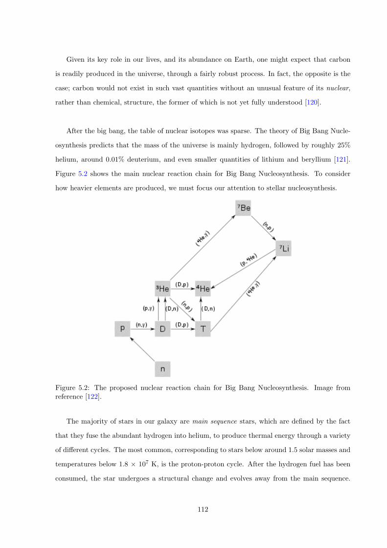
Given its key role in our lives, and its abundance on Earth, one might expect that carbon

is readily produced in the universe, through a fairly robust process. In fact, the opposite is the

case; carbon would not exist in such vast quantities without an unusual feature of its nuclear,

rather than chemical, structure, the former of which is not yet fully understood [120].

After the big bang, the table of nuclear isotopes was sparse. The theory of Big Bang Nucle-

osynthesis predicts that the mass of the universe is mainly hydrogen, followed by roughly 25%

helium, around 0.01% deuterium, and even smaller quantities of lithium and beryllium [121].

Figure 5.2 shows the main nuclear reaction chain for Big Bang Nucleosynthesis. To consider

how heavier elements are produced, we must focus our attention to stellar nucleosynthesis.

Figure 5.2: The proposed nuclear reaction chain for Big Bang Nucleosynthesis. Image fromreference [122].

The majority of stars in our galaxy are main sequence stars, which are defined by the fact

that they fuse the abundant hydrogen into helium, to produce thermal energy through a variety

of di↵erent cycles. The most common, corresponding to stars below around 1.5 solar masses and

temperatures below 1.8 ⇥ 107 K, is the proton-proton cycle. After the hydrogen fuel has been

consumed, the star undergoes a structural change and evolves away from the main sequence.

112

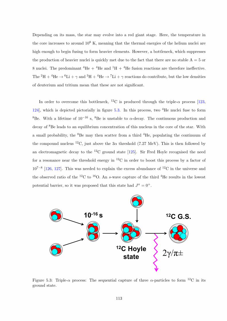
Depending on its mass, the star may evolve into a red giant stage. Here, the temperature in

the core increases to around 108 K, meaning that the thermal energies of the helium nuclei are

high enough to begin fusing to form heavier elements. However, a bottleneck, which suppresses

the production of heavier nuclei is quickly met due to the fact that there are no stable A = 5 or

8 nuclei. The predominant 4He + 4He and 1H + 4He fusion reactions are therefore ine↵ective.

The 2H + 4He ! 6Li + � and 3H + 4He ! 7Li + � reactions do contribute, but the low densities

of deuterium and tritium mean that these are not significant.

In order to overcome this bottleneck, 12C is produced through the triple-↵ process [123,

124], which is depicted pictorially in figure 5.3. In this process, two 4He nuclei fuse to form

8Be. With a lifetime of 10�16 s, 8Be is unstable to ↵-decay. The continuous production and

decay of 8Be leads to an equilibrium concentration of this nucleus in the core of the star. With

a small probability, the 8Be may then scatter from a third 4He, populating the continuum of

the compound nucleus 12C, just above the 3↵ threshold (7.27 MeV). This is then followed by

an electromagnetic decay to the 12C ground state [125]. Sir Fred Hoyle recognised the need

for a resonance near the threshold energy in 12C in order to boost this process by a factor of

107�8 [126, 127]. This was needed to explain the excess abundance of 12C in the universe and

the observed ratio of the 12C to 16O. An s-wave capture of the third 4He results in the lowest

potential barrier, so it was proposed that this state had J⇡ = 0+.

10-16 s

12C Hoyle state

12C G.S.

2γ/π±

Figure 5.3: Triple-↵ process: The sequential capture of three ↵-particles to form 12C in itsground state.

113

The energy of the Hoyle state was measured around the same time as Hoyle’s assertion [128],

partly due to his insistence when working as a visiting academic at Caltech. Its angular momen-

tum and parity were confirmed shortly later [129]. However, a state around the correct energy

in 12C was measured several years earlier [130]. It has been suggested that Hoyle’s prediction

of the existence of a 7.65 MeV resonance was an excellent example of the anthropic principle

[131]. This principle states that since intelligent life exists, certain properties of the universe

must also exist. In other words, the 7.65 MeV resonance in 12C must exist for humans to be

comprehending it. Whether Sir Fred Hoyle utilised the anthropic principle to solve the carbon

production problem has been the subject of some debate [132]. Nevertheless, the existence of

the Hoyle state resonance in 12C just above the 3↵ threshold is crucial for the development of

carbon-based life in the universe.

Despite the success of the Hoyle state in resolving the carbon production problem, a new

puzzle emerged. It turns out that it is very di�cult to describe the Hoyle state using common

models of atomic nuclei, such as the famous, and rather successful, shell model. Owing to its

role in nucleosynthesis, it was soon proposed that this state could be described as a system of

interacting ↵-particles, where the degrees of freedom of individual nucleons are not important

[133].

Despite 60 years of theoretical and experimental study, the nature of the Hoyle State in 12C

has not been well elucidated. Even if the state is ↵-clustered, what geometric configuration do

the ↵-particles take? Does it exist as a superposition of shell-model-like and ↵-cluster-like states?

Or could the underlying fermionic degrees of freedom of individual nucleons be ignored, opening

the possibility that the Hoyle state is the nuclear analogue of a Bose-Einstein condensate? The

following pages begin by discussing the role of the Hoyle state in stellar helium burning in

more detail. Some theoretical models that are used to describe the structure of the Hoyle state

are then discussed, along with their sometimes conflicting conclusions. Ways to experimentally

examine the structure of this state are also described, along with the insight that measuring its

direct decay could provide. The experiment that was performed to measure the direct decay

branch using the 12C(↵,↵)3↵ reaction in complete kinematics, is described in detail. The results

and implications for the structure of the Hoyle state are then discussed.

114

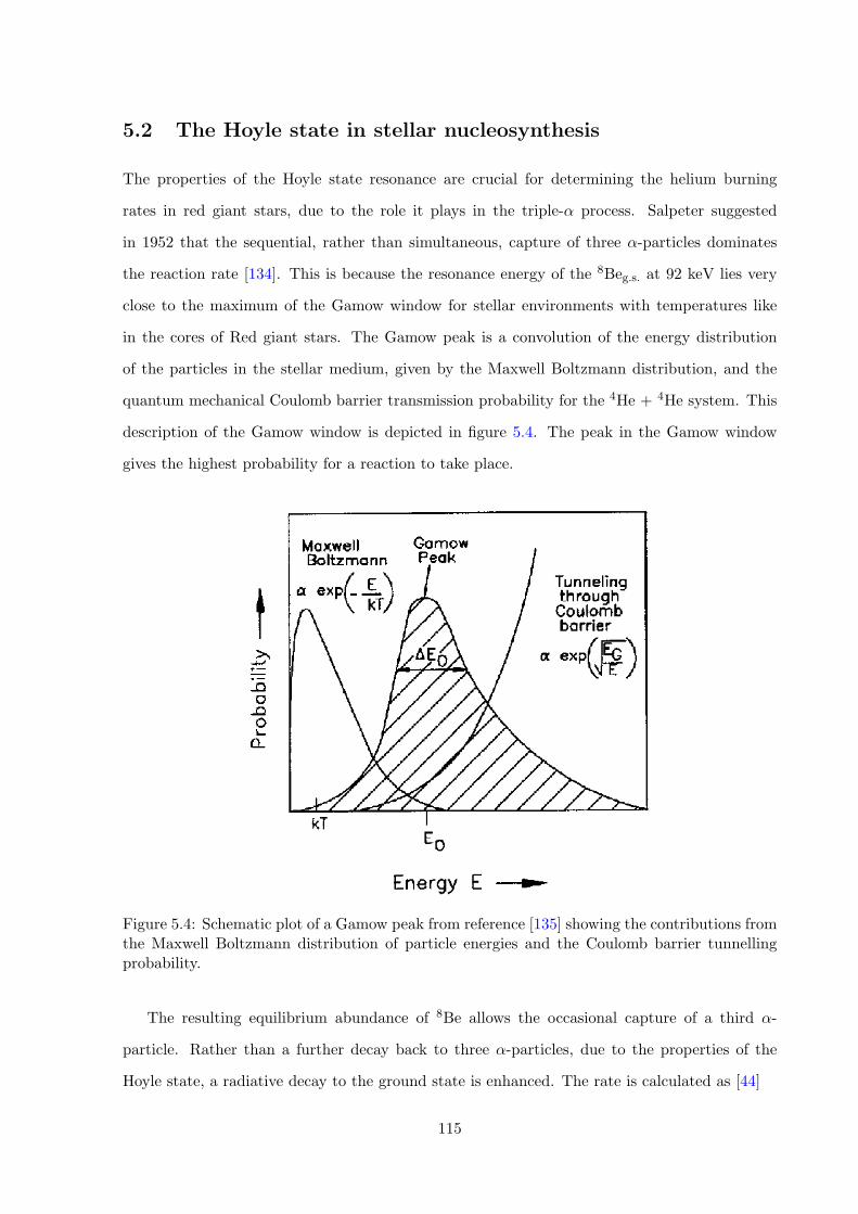
5.2 The Hoyle state in stellar nucleosynthesis

The properties of the Hoyle state resonance are crucial for determining the helium burning

rates in red giant stars, due to the role it plays in the triple-↵ process. Salpeter suggested

in 1952 that the sequential, rather than simultaneous, capture of three ↵-particles dominates

the reaction rate [134]. This is because the resonance energy of the 8Beg.s. at 92 keV lies very

close to the maximum of the Gamow window for stellar environments with temperatures like

in the cores of Red giant stars. The Gamow peak is a convolution of the energy distribution

of the particles in the stellar medium, given by the Maxwell Boltzmann distribution, and the

quantum mechanical Coulomb barrier transmission probability for the 4He + 4He system. This

description of the Gamow window is depicted in figure 5.4. The peak in the Gamow window

gives the highest probability for a reaction to take place.

Figure 5.4: Schematic plot of a Gamow peak from reference [135] showing the contributions fromthe Maxwell Boltzmann distribution of particle energies and the Coulomb barrier tunnellingprobability.

The resulting equilibrium abundance of 8Be allows the occasional capture of a third ↵-

particle. Rather than a further decay back to three ↵-particles, due to the properties of the

Hoyle state, a radiative decay to the ground state is enhanced. The rate is calculated as [44]

115

R / T�3/2�↵�rad.�tot.

exp�ER/kBT . (5.1)

The parameters �↵ and �rad. represent the Hoyle state ↵ and combined radiative widths,

respectively. The temperature is given by T and the energy of the resonance above the 3↵

threshold is ER. The total width of the state, �tot., is the sum of all of the partial widths. The

above equation assumes that the only contribution to the ↵ width is the 8Beg.s. + ↵ channel.

However, the width for the direct 3↵ reaction, �3↵, must also be considered. Since the probability

of the convergence of three ↵-particles simultaneously is incredibly small, this channel is unlikely

to contribute to the formation of 12C at these temperatures. However, since this direct width

contributes to the denominator of the term

�↵�rad.�tot.

=�↵+8Be�rad.

�↵+8Be + �rad. + �3↵, (5.2)

the inclusion of a non-zero direct 3↵ contribution will decrease the reaction rate. Therefore, a

precision measurement of the �3↵/�tot. quantity is needed. The triple-↵ reaction rate is still

much debated. A continuum-discretised coupled channel reaction calculation (CDCC) predicted

a significantly higher 3↵ reaction rate below 108 K [136]. This calculated that the s-wave res-

onances in the sequential ↵ capture reactions do not dominate at low T , and that the direct

3↵ reaction becomes more important. As shall be seen in section 5.5.1, the Coulomb barrier

tunnelling probability can be much lower for the simultaneous confluence of three ↵-particles

compared with the sequential capture, and therefore becomes more significant at lower temper-

atures. Direct reactions at lower temperatures will depend on the value of �3↵.

A number of recent experimental studies have measured the direct 3↵ decay width of the

Hoyle state. Raduta et al. calculated a 17% direct decay branch [137], which would a↵ect

the calculated triple-↵ reaction rate by several orders of magnitude. Several other studies have

placed limits on the direct decay branch at much lower levels, the lowest being 0.2% [138–140].

The experiment presented in this chapter builds on these latter studies.

116

5.3 Theoretical models of 12C and the Hoyle state

A wide variety of theoretical models have been used to try to understand the structure of

12C. Many of these have been covered in the general introduction to nuclear structure models

in section 2. Therefore, rather than providing in-depth explanations of the calculations, this

section will review their successes and failures when applied to the 12C nucleus.

5.3.1 Mean field models of 12C

At one end of the spectrum lies the description of the atomic nucleus in terms of a mean field

interaction, set up by the presence of all of the nucleons. In typical shell-model calculations,

the valence nucleons, which lie above a closed shell, are allowed to interact with one another

and dominate the dynamics of the nucleus. The nucleons lying below the shell closure are said

to form part of the inert core. As illustrated in figure 5.5 [141], these type of calculations well-

reproduce the binding energy of the ground state, and the excitations of the 4.4 MeV 2+ and 9.6

MeV 3� levels, suggesting that these states have a similar structure, which is well described by

the single-particle picture. On the other hand, the second 0+ state in these calculations (Hoyle

state) is systematically under-bound by several MeV, suggesting that it has a di↵erent structure.

The various columns in figure 5.5 compare the experimental levels (leftmost column) with

shell-model calculations, which utilise di↵erent two nucleon (NN) interactions. They only per-

mit valence nucleons to contribute to the excitation spectrum. Importantly, these calculations

are linked by their rather limited shell-model basis. The rightmost column used the Cohen

and Kurath (CK) interaction (0p-shell) to calculate the positive parity states and the Millener

and Curath (MK) interaction (p-s-d-shell) was used for the negative parity states [142]. The

calculations of reference [141] use their own derived MK3W interaction using a slightly larger

2h! and 3h! model space for the positive and negative parity solutions respectively.

117

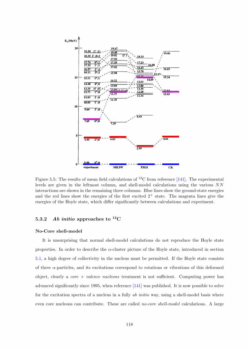
Figure 5.5: The results of mean field calculations of 12C from reference [141]. The experimentallevels are given in the leftmost column, and shell-model calculations using the various NNinteractions are shown in the remaining three columns. Blue lines show the ground-state energiesand the red lines show the energies of the first excited 2+ state. The magenta lines give theenergies of the Hoyle state, which di↵er significantly between calculations and experiment.

5.3.2 Ab initio approaches to 12C

No-Core shell-model

It is unsurprising that normal shell-model calculations do not reproduce the Hoyle state

properties. In order to describe the ↵-cluster picture of the Hoyle state, introduced in section

5.1, a high degree of collectivity in the nucleus must be permitted. If the Hoyle state consists

of three ↵-particles, and its excitations correspond to rotations or vibrations of this deformed

object, clearly a core + valence nucleons treatment is not su�cient. Computing power has

advanced significantly since 1995, when reference [141] was published. It is now possible to solve

for the excitation spectra of a nucleus in a fully ab initio way, using a shell-model basis where

even core nucleons can contribute. These are called no-core shell-model calculations. A large

118

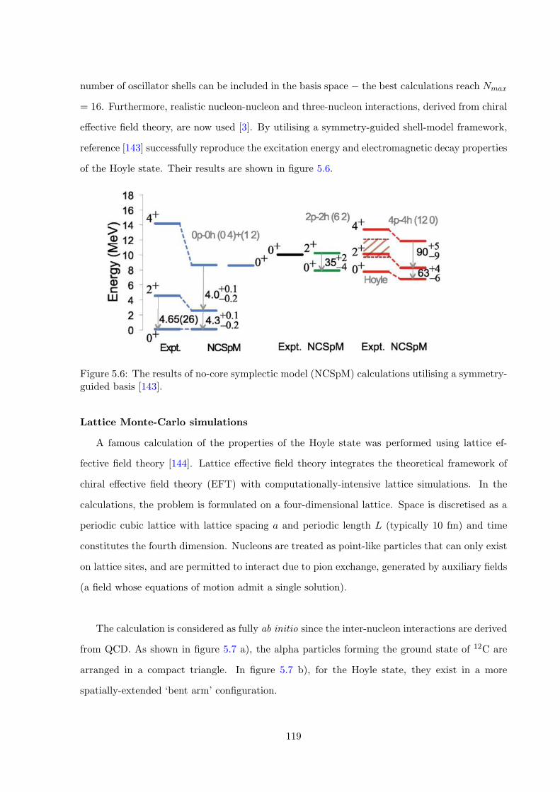
number of oscillator shells can be included in the basis space � the best calculations reach Nmax

= 16. Furthermore, realistic nucleon-nucleon and three-nucleon interactions, derived from chiral

e↵ective field theory, are now used [3]. By utilising a symmetry-guided shell-model framework,

reference [143] successfully reproduce the excitation energy and electromagnetic decay properties

of the Hoyle state. Their results are shown in figure 5.6.

Figure 5.6: The results of no-core symplectic model (NCSpM) calculations utilising a symmetry-guided basis [143].

Lattice Monte-Carlo simulations

A famous calculation of the properties of the Hoyle state was performed using lattice ef-

fective field theory [144]. Lattice e↵ective field theory integrates the theoretical framework of

chiral e↵ective field theory (EFT) with computationally-intensive lattice simulations. In the

calculations, the problem is formulated on a four-dimensional lattice. Space is discretised as a

periodic cubic lattice with lattice spacing a and periodic length L (typically 10 fm) and time

constitutes the fourth dimension. Nucleons are treated as point-like particles that can only exist

on lattice sites, and are permitted to interact due to pion exchange, generated by auxiliary fields

(a field whose equations of motion admit a single solution).

The calculation is considered as fully ab initio since the inter-nucleon interactions are derived

from QCD. As shown in figure 5.7 a), the alpha particles forming the ground state of 12C are

arranged in a compact triangle. In figure 5.7 b), for the Hoyle state, they exist in a more

spatially-extended ‘bent arm’ configuration.

119

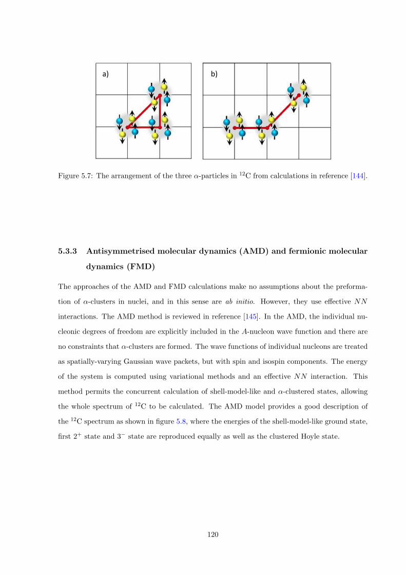
a) b)

Figure 5.7: The arrangement of the three ↵-particles in 12C from calculations in reference [144].

5.3.3 Antisymmetrised molecular dynamics (AMD) and fermionic molecular

dynamics (FMD)

The approaches of the AMD and FMD calculations make no assumptions about the preforma-

tion of ↵-clusters in nuclei, and in this sense are ab initio. However, they use e↵ective NN

interactions. The AMD method is reviewed in reference [145]. In the AMD, the individual nu-

cleonic degrees of freedom are explicitly included in the A-nucleon wave function and there are

no constraints that ↵-clusters are formed. The wave functions of individual nucleons are treated

as spatially-varying Gaussian wave packets, but with spin and isospin components. The energy

of the system is computed using variational methods and an e↵ective NN interaction. This

method permits the concurrent calculation of shell-model-like and ↵-clustered states, allowing

the whole spectrum of 12C to be calculated. The AMD model provides a good description of

the 12C spectrum as shown in figure 5.8, where the energies of the shell-model-like ground state,

first 2+ state and 3� state are reproduced equally as well as the clustered Hoyle state.

120

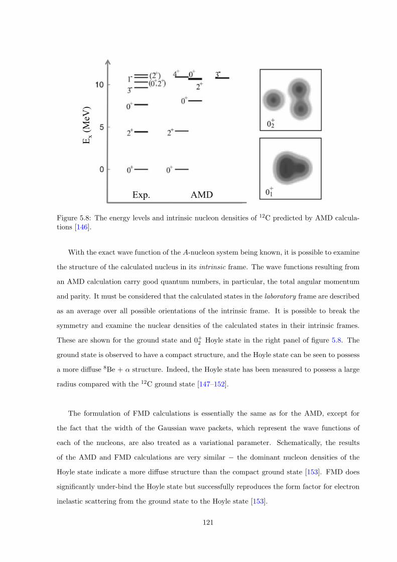
E x (M

eV)

Exp. AMD

Figure 5.8: The energy levels and intrinsic nucleon densities of 12C predicted by AMD calcula-tions [146].

With the exact wave function of the A-nucleon system being known, it is possible to examine

the structure of the calculated nucleus in its intrinsic frame. The wave functions resulting from

an AMD calculation carry good quantum numbers, in particular, the total angular momentum

and parity. It must be considered that the calculated states in the laboratory frame are described

as an average over all possible orientations of the intrinsic frame. It is possible to break the

symmetry and examine the nuclear densities of the calculated states in their intrinsic frames.

These are shown for the ground state and 0+2 Hoyle state in the right panel of figure 5.8. The

ground state is observed to have a compact structure, and the Hoyle state can be seen to possess

a more di↵use 8Be + ↵ structure. Indeed, the Hoyle state has been measured to possess a large

radius compared with the 12C ground state [147–152].

The formulation of FMD calculations is essentially the same as for the AMD, except for

the fact that the width of the Gaussian wave packets, which represent the wave functions of

each of the nucleons, are also treated as a variational parameter. Schematically, the results

of the AMD and FMD calculations are very similar � the dominant nucleon densities of the

Hoyle state indicate a more di↵use structure than the compact ground state [153]. FMD does

significantly under-bind the Hoyle state but successfully reproduces the form factor for electron

inelastic scattering from the ground state to the Hoyle state [153].

121

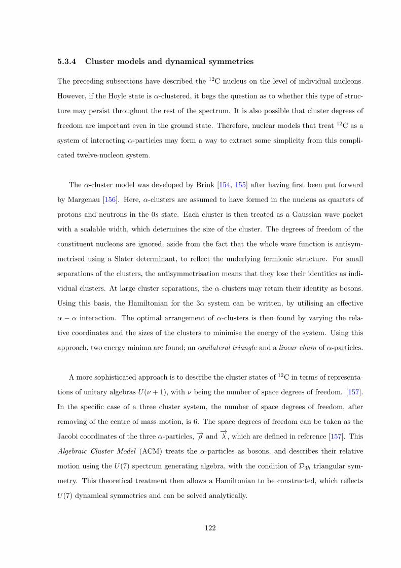
5.3.4 Cluster models and dynamical symmetries

The preceding subsections have described the 12C nucleus on the level of individual nucleons.

However, if the Hoyle state is ↵-clustered, it begs the question as to whether this type of struc-

ture may persist throughout the rest of the spectrum. It is also possible that cluster degrees of

freedom are important even in the ground state. Therefore, nuclear models that treat 12C as a

system of interacting ↵-particles may form a way to extract some simplicity from this compli-

cated twelve-nucleon system.

The ↵-cluster model was developed by Brink [154, 155] after having first been put forward

by Margenau [156]. Here, ↵-clusters are assumed to have formed in the nucleus as quartets of

protons and neutrons in the 0s state. Each cluster is then treated as a Gaussian wave packet

with a scalable width, which determines the size of the cluster. The degrees of freedom of the

constituent nucleons are ignored, aside from the fact that the whole wave function is antisym-

metrised using a Slater determinant, to reflect the underlying fermionic structure. For small

separations of the clusters, the antisymmetrisation means that they lose their identities as indi-

vidual clusters. At large cluster separations, the ↵-clusters may retain their identity as bosons.

Using this basis, the Hamiltonian for the 3↵ system can be written, by utilising an e↵ective

↵ � ↵ interaction. The optimal arrangement of ↵-clusters is then found by varying the rela-

tive coordinates and the sizes of the clusters to minimise the energy of the system. Using this

approach, two energy minima are found; an equilateral triangle and a linear chain of ↵-particles.

A more sophisticated approach is to describe the cluster states of 12C in terms of representa-

tions of unitary algebras U(⌫ + 1), with ⌫ being the number of space degrees of freedom. [157].

In the specific case of a three cluster system, the number of space degrees of freedom, after

removing of the centre of mass motion, is 6. The space degrees of freedom can be taken as the

Jacobi coordinates of the three ↵-particles, �!⇢ and�!� , which are defined in reference [157]. This

Algebraic Cluster Model (ACM) treats the ↵-particles as bosons, and describes their relative

motion using the U(7) spectrum generating algebra, with the condition of D3h triangular sym-

metry. This theoretical treatment then allows a Hamiltonian to be constructed, which reflects

U(7) dynamical symmetries and can be solved analytically.

122

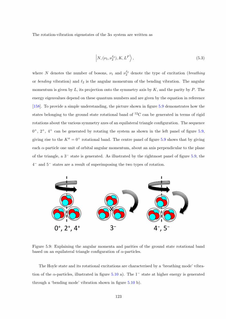
The rotation-vibration eigenstates of the 3↵ system are written as

���N, (⌫1, ⌫`2

2 ),K, LPE, (5.3)

where N denotes the number of bosons, ⌫1 and ⌫`22 denote the type of excitation (breathing

or bending vibration) and `2 is the angular momentum of the bending vibration. The angular

momentum is given by L, its projection onto the symmetry axis by K, and the parity by P . The

energy eigenvalues depend on these quantum numbers and are given by the equation in reference

[158]. To provide a simple understanding, the picture shown in figure 5.9 demonstrates how the

states belonging to the ground state rotational band of 12C can be generated in terms of rigid

rotations about the various symmetry axes of an equilateral triangle configuration. The sequence

0+, 2+, 4+ can be generated by rotating the system as shown in the left panel of figure 5.9,

giving rise to the K⇡ = 0+ rotational band. The centre panel of figure 5.9 shows that by giving

each ↵-particle one unit of orbital angular momentum, about an axis perpendicular to the plane

of the triangle, a 3� state is generated. As illustrated by the rightmost panel of figure 5.9, the

4� and 5� states are a result of superimposing the two types of rotation.

0+,2+,4+ 3− 4−,5−

Figure 5.9: Explaining the angular momenta and parities of the ground state rotational bandbased on an equilateral triangle configuration of ↵-particles.

The Hoyle state and its rotational excitations are characterised by a ‘breathing mode’ vibra-

tion of the ↵-particles, illustrated in figure 5.10 a). The 1� state at higher energy is generated

through a ‘bending mode’ vibration shown in figure 5.10 b).

123

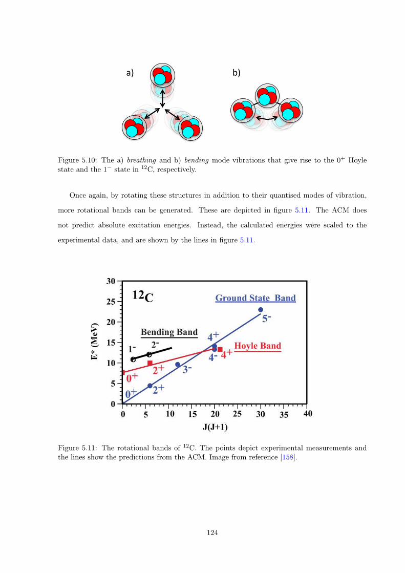
a) b)

Figure 5.10: The a) breathing and b) bending mode vibrations that give rise to the 0+ Hoylestate and the 1� state in 12C, respectively.

Once again, by rotating these structures in addition to their quantised modes of vibration,

more rotational bands can be generated. These are depicted in figure 5.11. The ACM does

not predict absolute excitation energies. Instead, the calculated energies were scaled to the

experimental data, and are shown by the lines in figure 5.11.

Figure 5.11: The rotational bands of 12C. The points depict experimental measurements andthe lines show the predictions from the ACM. Image from reference [158].

124

5.3.5 Bose-Einstein Condensates

Driven by developments in the field of cold atom physics [159] it has been hypothesised that the

Hoyle state corresponds to a dilute gas of ↵-particles [160]. The 0+ ↵-particle has the proper-

ties of a boson and the large physical size of the Hoyle state could allow the internal fermionic

degrees of freedom of the ↵-particles to be neglected. If this assumption were correct, then all

three ↵-particles would be able to occupy the lowest 0s state of their mean interaction potential.

In this sense, the state would be like a Bose-Einstein condensate (BEC). Nuclear ↵-condensates

would di↵er from their atomic BEC counterparts in many ways, and it is not yet fully clear how

the theory can be adapted to the context of a nucleus.

At around the time of the millennium, a number of theoretical studies investigated the pos-

sibility of an ↵-condensate state [161, 162]. They concluded that ↵-condensation would only

occur at a nuclear density around one fifth of the normal saturation density, and that at higher

densities nucleon-nucleon pairing would dominate. For a near-threshold state in an ↵-conjugate

nucleus, with an unusually large radius, the possibility of an ↵-condensation exists. Experiments

indicate that the Hoyle state may possess a nuclear volume up to four times larger than the

12C ground state [147–152], meaning that this state may be a good candidate for ↵-particle

condensation.

To theoretically describe such a structure, Tohsaki, Horiuchi, Schuck and Ropke adapted the

Brink wave function to reflect to possible condensate nature of this state [160, 163, 164]. On a

basic level, the wave function of an N↵ system is given as

|�N↵i =⇣C†↵

⌘N |vac.i . (5.4)

The creation operator, C†↵, is such that for a system of 12 nucleons

hr1, r2..., r12|�N↵i = A [�↵(r1..., r4)�↵(r5..., r8)�↵(r9..., r12)] . (5.5)

125

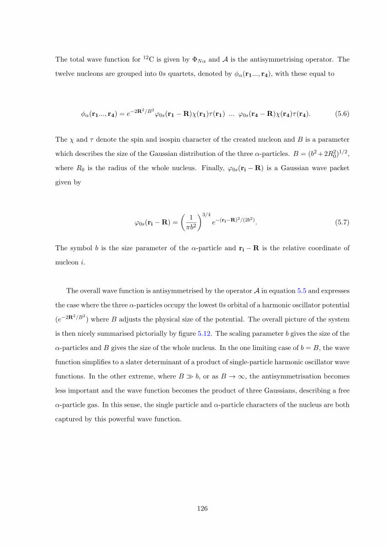
The total wave function for 12C is given by �N↵ and A is the antisymmetrising operator. The

twelve nucleons are grouped into 0s quartets, denoted by �↵(r1..., r4), with these equal to

�↵(r1..., r4) = e�2R2/B2

'0s(r1 �R)�(r1)⌧(r1) ... '0s(r4 �R)�(r4)⌧(r4). (5.6)

The � and ⌧ denote the spin and isospin character of the created nucleon and B is a parameter

which describes the size of the Gaussian distribution of the three ↵-particles. B = (b2+2R20)

1/2,

where R0 is the radius of the whole nucleus. Finally, '0s(ri �R) is a Gaussian wave packet

given by

'0s(ri �R) =

✓1

⇡b2

◆3/4

e�(ri�R)2/(2b2). (5.7)

The symbol b is the size parameter of the ↵-particle and ri �R is the relative coordinate of

nucleon i.

The overall wave function is antisymmetrised by the operator A in equation 5.5 and expresses

the case where the three ↵-particles occupy the lowest 0s orbital of a harmonic oscillator potential

(e�2R2/B2

) where B adjusts the physical size of the potential. The overall picture of the system

is then nicely summarised pictorially by figure 5.12. The scaling parameter b gives the size of the

↵-particles and B gives the size of the whole nucleus. In the one limiting case of b = B, the wave

function simplifies to a slater determinant of a product of single-particle harmonic oscillator wave

functions. In the other extreme, where B � b, or as B ! 1, the antisymmetrisation becomes

less important and the wave function becomes the product of three Gaussians, describing a free

↵-particle gas. In this sense, the single particle and ↵-particle characters of the nucleus are both

captured by this powerful wave function.

126

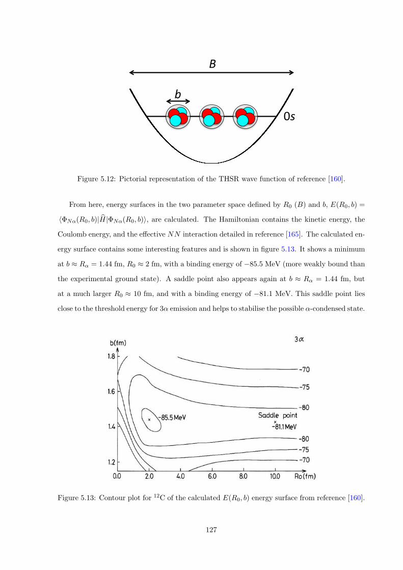
0s

b

B

Figure 5.12: Pictorial representation of the THSR wave function of reference [160].

From here, energy surfaces in the two parameter space defined by R0 (B) and b, E(R0, b) =

h�N↵(R0, b)| bH|�N↵(R0, b)i, are calculated. The Hamiltonian contains the kinetic energy, the

Coulomb energy, and the e↵ective NN interaction detailed in reference [165]. The calculated en-

ergy surface contains some interesting features and is shown in figure 5.13. It shows a minimum

at b ⇡ R↵ = 1.44 fm, R0 ⇡ 2 fm, with a binding energy of �85.5 MeV (more weakly bound than

the experimental ground state). A saddle point also appears again at b ⇡ R↵ = 1.44 fm, but

at a much larger R0 ⇡ 10 fm, and with a binding energy of �81.1 MeV. This saddle point lies

close to the threshold energy for 3↵ emission and helps to stabilise the possible ↵-condensed state.

Figure 5.13: Contour plot for 12C of the calculated E(R0, b) energy surface from reference [160].

127

A full quantum mechanical treatment of the 3↵ system was then performed, using b = 1.44

fm, and treating R0 as a discretised variable in the generator coordinate method [166]. This

allows the estimation of the values of the variational parameter R0 for the di↵erent states of

the system. The lowest 0+1 state corresponds to the 12C ground state. It is more unbound

than the experimentally-measured ground-state energy but has a similar RMS radius at 2.97 fm

(exp. = 2.65 fm). The next 0+2 excited state lies at 7.65 MeV excitation but has a much larger

calculated radius of 4.29 fm. This corresponds to a factor of three increase in the nuclear volume

compared with the calculated ground state and a factor of five greater than the experimental

ground state volume. Therefore, the second 0+2 Hoyle state corresponds to a very dilute system

of low density, suggesting that an ↵-condensate may exist.

A major success of the THSR approach is that it reproduces the absolute values of the charge

form factor for inelastic electron excitation from the ground state to the Hoyle state [167]. This

excellent agreement with experimental data indicates that the Hoyle state is indeed a large,

di↵use system and strongly influenced by the ↵-particle structure. The decomposition of the

THSR 0+2 wave function into the ↵-particle orbitals reveals a 70% overlap with the wave function

for three ↵-particles occupying the lowest 0s-orbital, indicating that the picture presented by

figure 5.12 is a reasonable approximation of the Hoyle state [168]. Conversely, the 12C ground

state shows a largely fragmented occupation of the ↵-particle orbitals, illustrating that the ↵-

particles lose their identities in the more compact ground state, as would be expected from the

antisymmetrisation.

128

5.4 The 3↵ decay of the Hoyle state

One way to examine the size of the Hoyle state is through electron inelastic scattering as was

discussed in section 5.3.5. However, an alternative, powerful probe into the size and structure of

the Hoyle state may be to consider the ways that it decays into three ↵-particles. This is also im-

portant for astrophysical calculations as discussed in section 5.2. Using intensity interferometry

techniques [169], it has been proposed that the size of a decaying nucleus could be determined

by quantum statistics and the final state Coulomb interactions of the emitted particles. The

emission of ↵-particles from 12C is, in principle, sensitive to the initial geometric arrangements

of these ↵-particles in the nucleus, prior to decay. Considering the sequential decay of 12C !8Beg.s. + ↵, the Coulomb repulsion between the first emitted particle and the two from the

subsequent decay of the 8Be, should perturb their relative velocities as they separate.

Freer showed in 2007, that for this channel, the Coulomb imprint in the relative velocity spec-

trum is lost, since the lifetime of the 8Beg.s. is around 10�16 s [170]. When the two ↵-particles

emerge from the decay of 8Be, they are su�ciently far from the first emitted ↵-particle that the

Coulomb field is weak, and the di↵erences in their final-state interactions become negligible. For

sequential decays of higher energy states in 12C through the short-lived excited 8Be2+ (width ⇡1.5 MeV), it has been shown that final-state Coulomb interactions are important in describing

experimental data [171–173]. Here, the decay of the short-lived intermediate state happens close

to the first emitted ↵-particle, meaning that the energies of the particles as they separate are

more sensitive to the Coulomb interaction.

The situation most sensitive to the Coulomb influences of each of the ↵-particles is that of

a direct decay, where all three particles are emitted simultaneously from the 12C nucleus, and

no intermediate resonances are formed. As discussed later in section 5.5.2, the direct decay is

rare since its phase space is severely hindered compared with the sequential decay process. The

preceding paragraphs have discussed that under a direct decay process, the relative energies of

the three emitted ↵-particles are sensitive to the initial configuration of the ↵-particles in 12C.

Now, various potential Hoyle state structures are discussed along with what their corresponding

↵ energy signatures could be under a direct decay process.

129

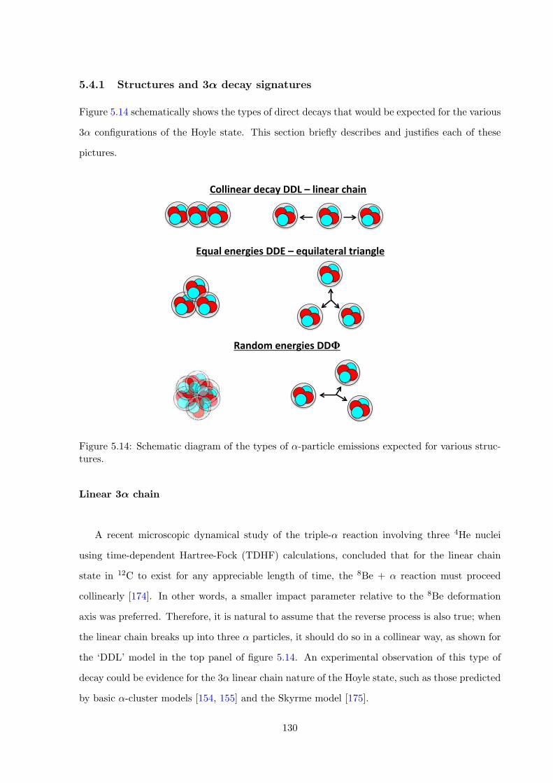
5.4.1 Structures and 3↵ decay signatures

Figure 5.14 schematically shows the types of direct decays that would be expected for the various

3↵ configurations of the Hoyle state. This section briefly describes and justifies each of these

pictures.

EqualenergiesDDE–equilateraltriangle

CollineardecayDDL–linearchain

RandomenergiesDDΦ

Figure 5.14: Schematic diagram of the types of ↵-particle emissions expected for various struc-tures.

Linear 3↵ chain

A recent microscopic dynamical study of the triple-↵ reaction involving three 4He nuclei

using time-dependent Hartree-Fock (TDHF) calculations, concluded that for the linear chain

state in 12C to exist for any appreciable length of time, the 8Be + ↵ reaction must proceed

collinearly [174]. In other words, a smaller impact parameter relative to the 8Be deformation

axis was preferred. Therefore, it is natural to assume that the reverse process is also true; when

the linear chain breaks up into three ↵ particles, it should do so in a collinear way, as shown for

the ‘DDL’ model in the top panel of figure 5.14. An experimental observation of this type of

decay could be evidence for the 3↵ linear chain nature of the Hoyle state, such as those predicted

by basic ↵-cluster models [154, 155] and the Skyrme model [175].

130

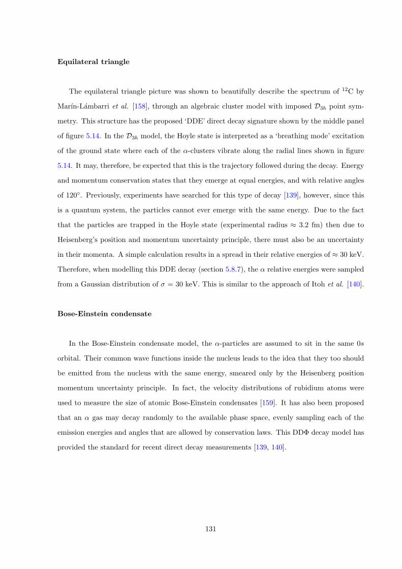
Equilateral triangle

The equilateral triangle picture was shown to beautifully describe the spectrum of 12C by

Marın-Lambarri et al. [158], through an algebraic cluster model with imposed D3h point sym-

metry. This structure has the proposed ‘DDE’ direct decay signature shown by the middle panel

of figure 5.14. In the D3h model, the Hoyle state is interpreted as a ‘breathing mode’ excitation

of the ground state where each of the ↵-clusters vibrate along the radial lines shown in figure

5.14. It may, therefore, be expected that this is the trajectory followed during the decay. Energy

and momentum conservation states that they emerge at equal energies, and with relative angles

of 120�. Previously, experiments have searched for this type of decay [139], however, since this

is a quantum system, the particles cannot ever emerge with the same energy. Due to the fact

that the particles are trapped in the Hoyle state (experimental radius ⇡ 3.2 fm) then due to

Heisenberg’s position and momentum uncertainty principle, there must also be an uncertainty

in their momenta. A simple calculation results in a spread in their relative energies of ⇡ 30 keV.

Therefore, when modelling this DDE decay (section 5.8.7), the ↵ relative energies were sampled

from a Gaussian distribution of � = 30 keV. This is similar to the approach of Itoh et al. [140].

Bose-Einstein condensate

In the Bose-Einstein condensate model, the ↵-particles are assumed to sit in the same 0s

orbital. Their common wave functions inside the nucleus leads to the idea that they too should

be emitted from the nucleus with the same energy, smeared only by the Heisenberg position

momentum uncertainty principle. In fact, the velocity distributions of rubidium atoms were

used to measure the size of atomic Bose-Einstein condensates [159]. It has also been proposed

that an ↵ gas may decay randomly to the available phase space, evenly sampling each of the

emission energies and angles that are allowed by conservation laws. This DD� decay model has

provided the standard for recent direct decay measurements [139, 140].

131

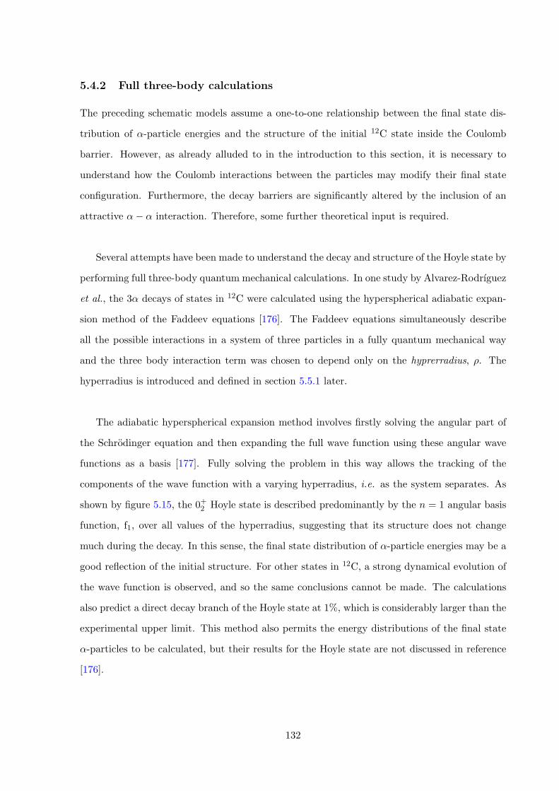
5.4.2 Full three-body calculations

The preceding schematic models assume a one-to-one relationship between the final state dis-

tribution of ↵-particle energies and the structure of the initial 12C state inside the Coulomb

barrier. However, as already alluded to in the introduction to this section, it is necessary to

understand how the Coulomb interactions between the particles may modify their final state

configuration. Furthermore, the decay barriers are significantly altered by the inclusion of an

attractive ↵� ↵ interaction. Therefore, some further theoretical input is required.

Several attempts have been made to understand the decay and structure of the Hoyle state by

performing full three-body quantum mechanical calculations. In one study by Alvarez-Rodrıguez

et al., the 3↵ decays of states in 12C were calculated using the hyperspherical adiabatic expan-

sion method of the Faddeev equations [176]. The Faddeev equations simultaneously describe

all the possible interactions in a system of three particles in a fully quantum mechanical way

and the three body interaction term was chosen to depend only on the hyprerradius, ⇢. The

hyperradius is introduced and defined in section 5.5.1 later.

The adiabatic hyperspherical expansion method involves firstly solving the angular part of

the Schrodinger equation and then expanding the full wave function using these angular wave

functions as a basis [177]. Fully solving the problem in this way allows the tracking of the

components of the wave function with a varying hyperradius, i.e. as the system separates. As

shown by figure 5.15, the 0+2 Hoyle state is described predominantly by the n = 1 angular basis

function, f1, over all values of the hyperradius, suggesting that its structure does not change

much during the decay. In this sense, the final state distribution of ↵-particle energies may be a

good reflection of the initial structure. For other states in 12C, a strong dynamical evolution of

the wave function is observed, and so the same conclusions cannot be made. The calculations

also predict a direct decay branch of the Hoyle state at 1%, which is considerably larger than the

experimental upper limit. This method also permits the energy distributions of the final state

↵-particles to be calculated, but their results for the Hoyle state are not discussed in reference

[176].

132

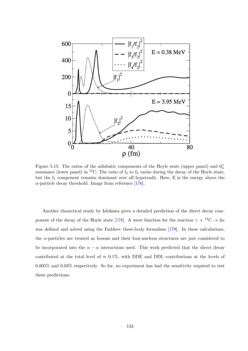
Figure 5.15: The ratios of the adiabatic components of the Hoyle state (upper panel) and 0+3resonance (lower panel) in 12C. The ratio of f2 to f3 varies during the decay of the Hoyle state,but the f1 component remains dominant over all hyperradii. Here, E is the energy above the↵-particle decay threshold. Image from reference [176].

Another theoretical study by Ishikawa gives a detailed prediction of the direct decay com-

ponent of the decay of the Hoyle state [178]. A wave function for the reaction � + 12C ! 3↵

was defined and solved using the Faddeev three-body formalism [179]. In these calculations,

the ↵-particles are treated as bosons and their four-nucleon structures are just considered to

be incorporated into the ↵ � ↵ interactions used. This work predicted that the direct decay

contributed at the total level of ⇡ 0.1%, with DDE and DDL contributions at the levels of

0.005% and 0.03% respectively. So far, no experiment has had the sensitivity required to test

these predictions.

133

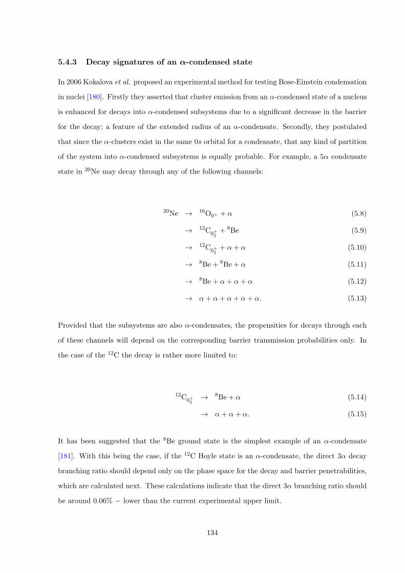
5.4.3 Decay signatures of an ↵-condensed state

In 2006 Kokalova et al. proposed an experimental method for testing Bose-Einstein condensation

in nuclei [180]. Firstly they asserted that cluster emission from an ↵-condensed state of a nucleus

is enhanced for decays into ↵-condensed subsystems due to a significant decrease in the barrier

for the decay; a feature of the extended radius of an ↵-condensate. Secondly, they postulated

that since the ↵-clusters exist in the same 0s orbital for a condensate, that any kind of partition

of the system into ↵-condensed subsystems is equally probable. For example, a 5↵ condensate

state in 20Ne may decay through any of the following channels:

20Ne ! 16O0+ + ↵ (5.8)

! 12C0+2

+ 8Be (5.9)

! 12C0+2

+ ↵+ ↵ (5.10)

! 8Be + 8Be + ↵ (5.11)

! 8Be + ↵+ ↵+ ↵ (5.12)

! ↵+ ↵+ ↵+ ↵+ ↵. (5.13)

Provided that the subsystems are also ↵-condensates, the propensities for decays through each

of these channels will depend on the corresponding barrier transmission probabilities only. In

the case of the 12C the decay is rather more limited to:

12C0+2

! 8Be + ↵ (5.14)

! ↵+ ↵+ ↵. (5.15)

It has been suggested that the 8Be ground state is the simplest example of an ↵-condensate

[181]. With this being the case, if the 12C Hoyle state is an ↵-condensate, the direct 3↵ decay

branching ratio should depend only on the phase space for the decay and barrier penetrabilities,

which are calculated next. These calculations indicate that the direct 3↵ branching ratio should

be around 0.06% � lower than the current experimental upper limit.

134

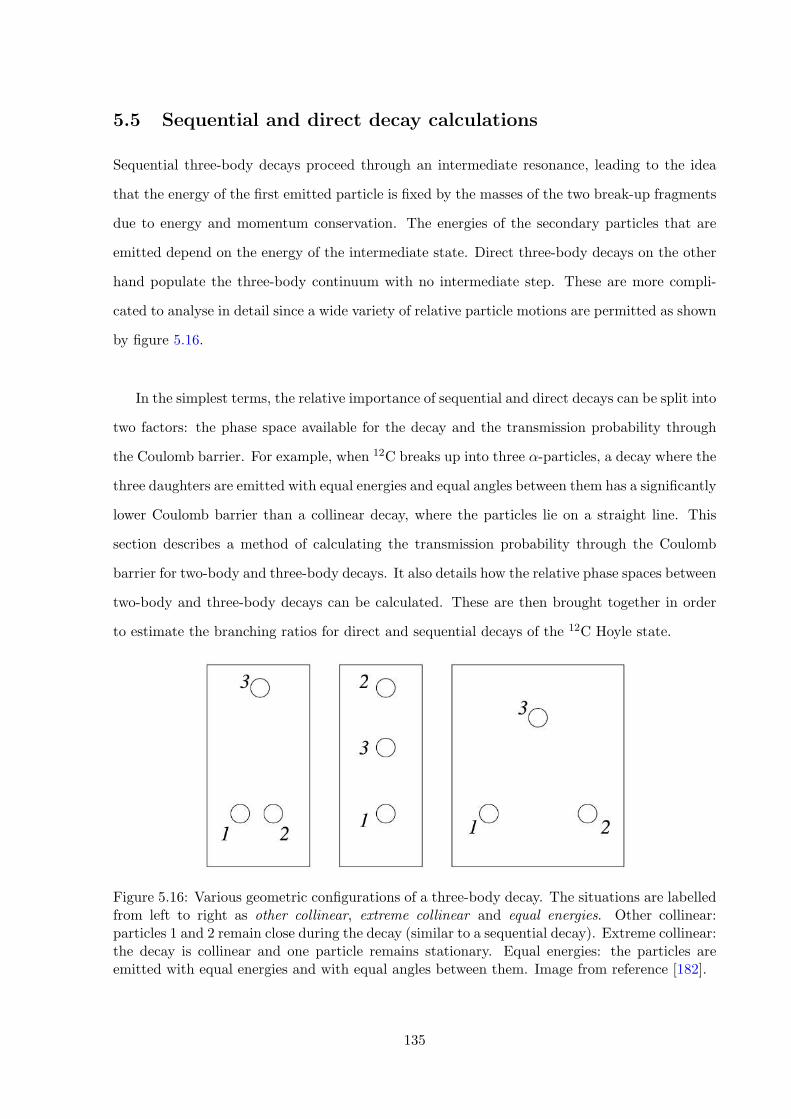
5.5 Sequential and direct decay calculations

Sequential three-body decays proceed through an intermediate resonance, leading to the idea

that the energy of the first emitted particle is fixed by the masses of the two break-up fragments

due to energy and momentum conservation. The energies of the secondary particles that are

emitted depend on the energy of the intermediate state. Direct three-body decays on the other

hand populate the three-body continuum with no intermediate step. These are more compli-

cated to analyse in detail since a wide variety of relative particle motions are permitted as shown

by figure 5.16.

In the simplest terms, the relative importance of sequential and direct decays can be split into

two factors: the phase space available for the decay and the transmission probability through

the Coulomb barrier. For example, when 12C breaks up into three ↵-particles, a decay where the

three daughters are emitted with equal energies and equal angles between them has a significantly

lower Coulomb barrier than a collinear decay, where the particles lie on a straight line. This

section describes a method of calculating the transmission probability through the Coulomb

barrier for two-body and three-body decays. It also details how the relative phase spaces between

two-body and three-body decays can be calculated. These are then brought together in order

to estimate the branching ratios for direct and sequential decays of the 12C Hoyle state.

Figure 5.16: Various geometric configurations of a three-body decay. The situations are labelledfrom left to right as other collinear, extreme collinear and equal energies. Other collinear:particles 1 and 2 remain close during the decay (similar to a sequential decay). Extreme collinear:the decay is collinear and one particle remains stationary. Equal energies: the particles areemitted with equal energies and with equal angles between them. Image from reference [182].

135

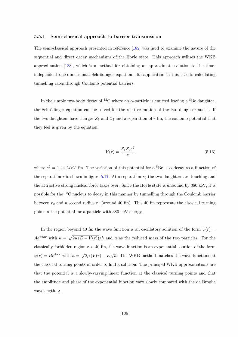
5.5.1 Semi-classical approach to barrier transmission

The semi-classical approach presented in reference [182] was used to examine the nature of the

sequential and direct decay mechanisms of the Hoyle state. This approach utilises the WKB

approximation [183], which is a method for obtaining an approximate solution to the time-

independent one-dimensional Schrodinger equation. Its application in this case is calculating

tunnelling rates through Coulomb potential barriers.

In the simple two-body decay of 12C where an ↵-particle is emitted leaving a 8Be daughter,

the Schrodinger equation can be solved for the relative motion of the two daughter nuclei. If

the two daughters have charges Z1 and Z2 and a separation of r fm, the coulomb potential that

they feel is given by the equation

V (r) =Z1Z2e

2

r, (5.16)

where e2 = 1.44 MeV fm. The variation of this potential for a 8Be + ↵ decay as a function of

the separation r is shown in figure 5.17. At a separation r0 the two daughters are touching and

the attractive strong nuclear force takes over. Since the Hoyle state is unbound by 380 keV, it is

possible for the 12C nucleus to decay in this manner by tunnelling through the Coulomb barrier

between r0 and a second radius r1 (around 40 fm). This 40 fm represents the classical turning

point in the potential for a particle with 380 keV energy.

In the region beyond 40 fm the wave function is an oscillatory solution of the form (r) =

Ae±ir with =p

2µ (E � V (r))/h and µ as the reduced mass of the two particles. For the

classically forbidden region r < 40 fm, the wave function is an exponential solution of the form

(r) = Be±r with =p2µ (V (r)� E)/h. The WKB method matches the wave functions at

the classical turning points in order to find a solution. The principal WKB approximations are

that the potential is a slowly-varying linear function at the classical turning points and that

the amplitude and phase of the exponential function vary slowly compared with the de Broglie

wavelength, �.

136

0 10 20 30 40 50 60r (fm)

0

0.5

1

1.5

2

2.5

3

V(r)

(MeV

)

Two-body V(r)Decay energyr0

r0

8Be α

Figure 5.17: The 8Be + ↵ Coulomb barrier as a function of the separation of the two fragments.

Under these approximations it can be derived that the tunnelling probability is given by the

equation

T =1

1 + e2S⇡ e�2S , where S =

1

h

Z r1

r0

drp2µ (V (r)� E). (5.17)

Based on the derivation in reference [182], for a Coulomb potential, this can be simplified to

S =⇡

2

�Z1Z2e

2�r

2µ

h2E. (5.18)

The equivalent calculation for a three-body decay is less simple due to the fact that each

particle must tunnel through a Coulomb barrier set up by all three particles, according to

equation 5.19. As the system moves apart during the decay, the potential changes in a more

complicated way, which depends on the relative directions of the three particles. With reference

to figure 5.18, the total Coulomb potential for a particular orientation of particles is given by

equations

137

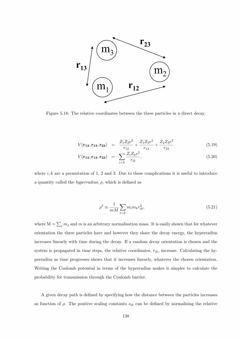
m1 m2

m3

r12

r23

r13

Figure 5.18: The relative coordinates between the three particles in a direct decay.

V (r12, r13, r23) =Z1Z2e

2

r12+

Z1Z3e2

r13+

Z2Z3e2

r23(5.19)

V (r12, r13, r23) =X

i<k

ZiZke2

rik, (5.20)

where i, k are a permutation of 1, 2 and 3. Due to these complications it is useful to introduce

a quantity called the hyperradius, ⇢, which is defined as

⇢2 ⌘ 1

mM

X

i<k

mimkr2ik, (5.21)

where M =P

j mj andm is an arbitrary normalisation mass. It is easily shown that for whatever

orientation the three particles have and however they share the decay energy, the hyperradius

increases linearly with time during the decay. If a random decay orientation is chosen and the

system is propagated in time steps, the relative coordinates, rik, increase. Calculating the hy-

perradius as time progresses shows that it increases linearly, whatever the chosen orientation.

Writing the Coulomb potential in terms of the hyperradius makes it simpler to calculate the

probability for transmission through the Coulomb barrier.

A given decay path is defined by specifying how the distance between the particles increases

as function of ⇢. The positive scaling constants sik can be defined by normalising the relative

138

distances between the particles by the hyperradius as

s2ik ⌘ r2ik⇢2

. (5.22)

These scaling constants, sik, provide a way to parameterise the geometry of the decay. Making

reference to figure 5.16, reading from left to right, if s13 ⇡ s23 and s12 ⇡ 0 then particles 1 and

2 remain close until particle 3 has travelled far away. This is almost equivalent to a sequential

decay. If s13 ⇡ s23 and s12 ⇡ s13 + s23, then we have a collinear decay where particle 3 remains

stationary. If s12 ⇡ s13 ⇡ s23 we have the case where the particles separate at equal angles to

one another.

The Coulomb potential can be parameterised by the hyperradius and scaling constants as

V (⇢) =X

i<k

ZiZke2

rik=

1

⇢

X

i<k

ZiZke2

sik. (5.23)

Therefore, for a general decay geometry, parameterised by the scaling constants, sik, the po-

tential barrier can be calculated as a function of ⇢. The Coulomb barriers corresponding to

the three geometries shown in figure 5.16 are plotted in figure 5.19. This shows an interesting

result. An ‘equal energies’ decay has the lowest Coulomb barrier. A totally collinear decay has

the largest Coulomb barrier. The barrier for a decay where two of the particles remain close

together (similar to a sequential decay) lies somewhere between the other two extremes.

The transmission probability is calculable using equation 5.23 as

T =1

1 + e2S⇡ e�2S where S =

1

h

Z ⇢1

⇢0

d⇢p2m (V (⇢)� E). (5.24)

139

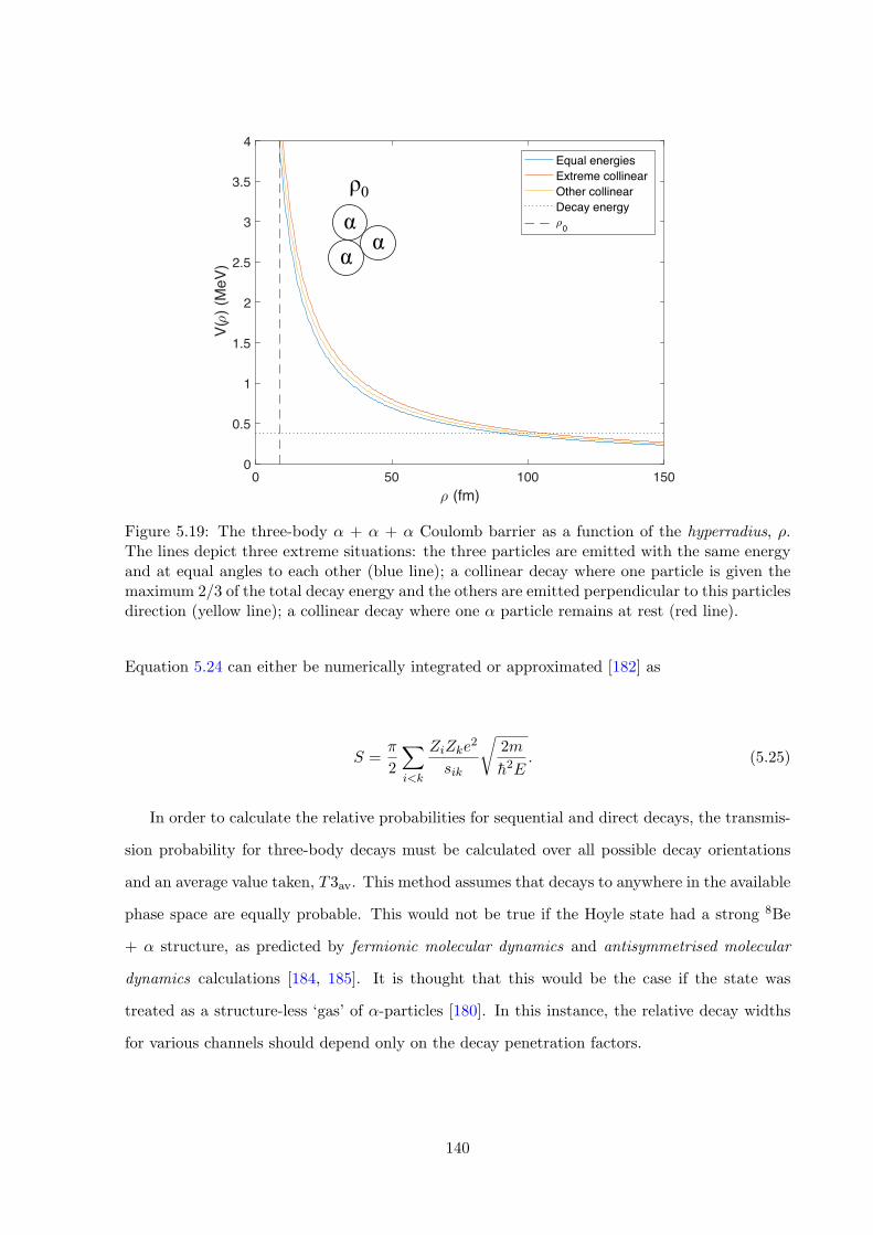
0 50 100 150� (fm)

0

0.5

1

1.5

2

2.5

3

3.5

4

V(�

) (M

eV)

Equal energiesExtreme collinearOther collinearDecay energy�0

α α α

ρ0

Figure 5.19: The three-body ↵ + ↵ + ↵ Coulomb barrier as a function of the hyperradius, ⇢.The lines depict three extreme situations: the three particles are emitted with the same energyand at equal angles to each other (blue line); a collinear decay where one particle is given themaximum 2/3 of the total decay energy and the others are emitted perpendicular to this particlesdirection (yellow line); a collinear decay where one ↵ particle remains at rest (red line).

Equation 5.24 can either be numerically integrated or approximated [182] as

S =⇡

2

X

i<k

ZiZke2

sik

r2m

h2E. (5.25)

In order to calculate the relative probabilities for sequential and direct decays, the transmis-

sion probability for three-body decays must be calculated over all possible decay orientations

and an average value taken, T3av. This method assumes that decays to anywhere in the available

phase space are equally probable. This would not be true if the Hoyle state had a strong 8Be

+ ↵ structure, as predicted by fermionic molecular dynamics and antisymmetrised molecular

dynamics calculations [184, 185]. It is thought that this would be the case if the state was

treated as a structure-less ‘gas’ of ↵-particles [180]. In this instance, the relative decay widths

for various channels should depend only on the decay penetration factors.

140

The Matlab code, given in reference [186], was written, which generates a large number

of random decay orientations for the three-body decay of 12C into three ↵-particles. These

are chosen to evenly sample the phase space while conserving energy and momentum. As is

discussed in references [139] and [140], and later in section 5.8.6, this corresponds to randomly

sampling the kinematically-allowed region of the symmetric Dalitz plot for the decay. The three-

body decay transmission probability, T3av, was calculated over 106 random geometries and the

average value was calculated. The two-body decay transmission probability, T2, for 8Be + ↵

was also calculated. The branching ratio for a direct decay was then calculated as

BR =T3av

T3av + T2⇡ 1/3. (5.26)

It has also been proposed that for an ↵-gas-like state, there is a propensity for the ↵-particles

to be emitted with similar energies as a reflection of their underlying identical wave functions

in the decaying nucleus [137]. In this case, three-body transmission probabilities should only be

calculated for decay geometries parameterised as s12 ⇡ s13 ⇡ s23. This results in a much higher

branching ratio BR ⇡ 6. The value quoted in equation 5.26 is therefore a lower limit on the

direct decay contribution.

However, caution should be taken when interpreting this value. As noted in reference [187],

this method treats the system from outside the range of the strong interaction meaning that

only Coulomb (and centrifugal) barriers remain. However, this assumes that the small distance

many-body dynamics is unimportant in the decay process. More advanced three-body models

include both the short range and the long range interactions in computing resonances [188, 189].

In the case of the Hoyle state, the width calculated using WKB methods was evaluated to be

around 60 eV. This is three times larger than the full computation [188] and about eight times

larger than the experimentally measured value of 8.5 eV [190].

Furthermore, to calculate the true value of the branching ratio, the magnitude of the relative

phases spaces available for sequential and direct decays must be calculated, which is discussed

in the next section.

141

5.5.2 Phase space calculations

To calculate the phase space for two-body and three-body decays, the Fermi break-up model

was used [191]. The break-up probability of a nucleus decaying into n fragments, excluding the

e↵ects of the Coulomb barrier penetration, is given by

W (E, n) =

✓V

⌦

◆n�1

⇢n(E), (5.27)

where, ⇢n(E) is the density of final states, ⌦ = (2⇡h)3 is the normalisation volume and V is

the volume of the decaying nucleus. Here, V is defined as 4⇡R30/3. The nuclear radius, R0, is

defined in the standard way R0 = 1.4A1/3.

In the Fermi break-up model, the density of final states is defined as

⇢n(E) = Mn(E)SnGn. (5.28)

The Sn term counts the number of states with di↵erent spin orientations. For n break-up

fragments, each of spin, sb, the Sn term is given by

Sn =nY

b=1

(2sb + 1) . (5.29)

For the decay of the Hoyle state to 8Be + ↵ or to 3↵, S2 = S3 = 1, since all of the fragments

are s = 0. The Gn term is called the permutation factor, which accounts for the identities of

the components in the final state to avoid double counting states. The number of particles of

type j is given by nj , and k is defined as the number of groups of identical particles. The Gn

term is given as

Gn =kY

j=1

1

nj !. (5.30)

142

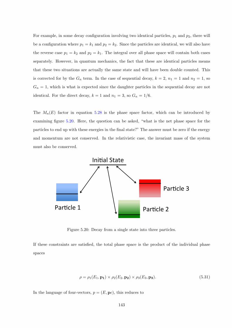
For example, in some decay configuration involving two identical particles, p1 and p2, there will

be a configuration where p1 = k1 and p2 = k2. Since the particles are identical, we will also have

the reverse case p1 = k2 and p2 = k1. The integral over all phase space will contain both cases

separately. However, in quantum mechanics, the fact that these are identical particles means

that these two situations are actually the same state and will have been double counted. This

is corrected for by the Gn term. In the case of sequential decay, k = 2, n1 = 1 and n2 = 1, so

Gn = 1, which is what is expected since the daughter particles in the sequential decay are not

identical. For the direct decay, k = 1 and n1 = 3, so Gn = 1/6.

The Mn(E) factor in equation 5.28 is the phase space factor, which can be introduced by

examining figure 5.20. Here, the question can be asked, “what is the net phase space for the

particles to end up with these energies in the final state?” The answer must be zero if the energy

and momentum are not conserved. In the relativistic case, the invariant mass of the system

must also be conserved.

Ini$alState

Par$cle1 Par$cle2

Par$cle3

Figure 5.20: Decay from a single state into three particles.

If these constraints are satisfied, the total phase space is the product of the individual phase

spaces

⇢ = ⇢1(E1,p1)⇥ ⇢2(E2,p2)⇥ ⇢3(E3,p3). (5.31)

In the language of four-vectors, p = (E,pc), this reduces to

143

⇢ = ⇢1(p1)⇥ ⇢2(p2)⇥ ⇢3(p3). (5.32)

To quantify the total phase space, all of the kinematically-allowed four-vectors must be integrated

over as

⇢tot =1

(2⇡)4

Z

allowedd4p1 d

4p2 d4p3 ⇢1(p1) ⇢2(p2) ⇢3(p3). (5.33)

To permit this, several Dirac delta � and Heaviside-Lorenz ⇥ functions must be used in the

integral to enforce the conservation laws. Therefore, in the case of an n-body decay, the integral

will have the form

⇢tot /Z�4(

nX

i

pi �nX

f

pf )nY

j=1

�(p2j �m2jc

2) ⇥(p0j ) d4(pj). (5.34)

This complicated-looking equation simply states that the phase space is evenly distributed over

all n final state particles, subject to energy, momentum and mass conservation. The first term,

�4(P

i pi �P

f pf ), ensures that energy and momentum are conserved between the initial and

final states. The product is over all outgoing particles. The �(p2j � m2jc

2) ensures that the

outgoing particles are on mass shell (real), and ⇥(p0j ) ensures that their energies are positive.

In the non-relativistic case, the integral can be solved analytically for an n-body decay [192] to

give

Mn(E, n) =

1Pn

b=1mb

nY

b=1

mb

!3/2(2⇡)3(n�1)/2

�(3(n� 1)/2)E3n/2�5/2, (5.35)

where � is the Gamma function, mb are the masses of each fragment and E is the decay energy.

Equation 5.27 was then evaluated and the ratio of the phase spaces for the two-body and three-

body decay of the Hoyle state was found to be W (E3, 3)/W (E2, 2) = 1.8 ⇥ 10�3. Combining

this with the relative transmission probabilities through the Coulomb barrier, detailed in section

144

5.5.1 (equation 5.26), gives a prediction for the direct decay branching ratio as 6 ⇥ 10�4 (0.06%).

This value is particularly applicable to an ↵-condensate structure for the Hoyle state, since the

decay of a condensate state into ↵-condensed subsystems should only depend on the phase space

and barrier penetrabilities.

145

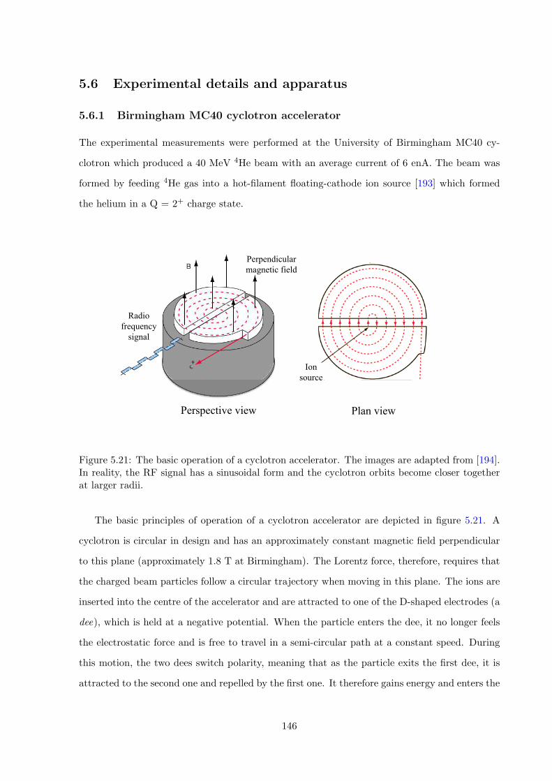
5.6 Experimental details and apparatus

5.6.1 Birmingham MC40 cyclotron accelerator

The experimental measurements were performed at the University of Birmingham MC40 cy-

clotron which produced a 40 MeV 4He beam with an average current of 6 enA. The beam was

formed by feeding 4He gas into a hot-filament floating-cathode ion source [193] which formed

the helium in a Q = 2+ charge state.

Ion source

Perpendicular magnetic field

Radio frequency

signal

Perspective view Plan view

Figure 5.21: The basic operation of a cyclotron accelerator. The images are adapted from [194].In reality, the RF signal has a sinusoidal form and the cyclotron orbits become closer togetherat larger radii.

The basic principles of operation of a cyclotron accelerator are depicted in figure 5.21. A

cyclotron is circular in design and has an approximately constant magnetic field perpendicular

to this plane (approximately 1.8 T at Birmingham). The Lorentz force, therefore, requires that

the charged beam particles follow a circular trajectory when moving in this plane. The ions are

inserted into the centre of the accelerator and are attracted to one of the D-shaped electrodes (a

dee), which is held at a negative potential. When the particle enters the dee, it no longer feels

the electrostatic force and is free to travel in a semi-circular path at a constant speed. During

this motion, the two dees switch polarity, meaning that as the particle exits the first dee, it is

attracted to the second one and repelled by the first one. It therefore gains energy and enters the

146

second dee. Again, it travels in a semi-circular path but with a slightly larger radius. Driving

the potential on the dees at the aptly named cyclotron frequency, given in equation 5.38, means

that this acceleration process happens a number of times, accelerating the particle to higher and

higher energies until its orbital radius reaches the edge of the accelerator, where it is extracted.

The cyclotron frequency is derived by firstly equating the centripetal force experienced by an

ion, with the Lorentz force, which is maintaining its circular trajectory.

mv2

r= qv|�!B |, (5.36)

=>v

r=

q|�!B |m

. (5.37)

The time period of a single cyclotron orbit can be identified as 2⇡r/v, hence, the angular

frequency is given as

! =q|�!B |2⇡m

. (5.38)

Given a particular magnetic field strength�!B and extraction radius R0, the energy of an

accelerated particle of mass m and charge q, in the non-relativistic limit, is given by

E0 =q2|�!B |2R2

0

2m. (5.39)

At relativistic energies, the mass of the ion increases, meaning that its motion moves out

of phase with the driving frequency of the dees. This can be corrected for by utilising a more

complicated magnetic field (Azimuthally Varying Field cyclotrons).

The Birmingham MC40 cyclotron is designed slightly di↵erently to this simplistic picture

[195]. The particle orbit is split into four quadrants. The alternating voltage is applied to two

90 degree ‘half-dee’ cavities which are mounted radially opposite each other, while the other two

‘dummy dees’ are held at ground potential. This means that ions are accelerated four times on

147

each orbit, which in turn permits a wider range of ions and energies that can be accelerated

using the limited range of frequencies available from the RF source. Further subtleties such as

an azimuthally-varying field to aid beam focusing are also present. The beam energy depends

on the radius of beam extraction. This can vary by 1-2 mm and leads to a typical 100-300 keV

uncertainty [82].

The name, MC40, originates from the fact that this machine can accelerate protons up to 40

MeV. This is called the k-number and has a value of 40. Given equation 5.39, this fact may be

used as a calibration to calculate the maximum energies achievable for a range of ions of mass

mi and charge state qi, as

Ei = 40⇥ q2iq2p

mp

miMeV. (5.40)

Upon extraction from the accelerator, the beam was directed towards the target and mea-

surement apparatus using the Vivitron 12-way switching magnet, from Strasbourg, installed in

2005.

148

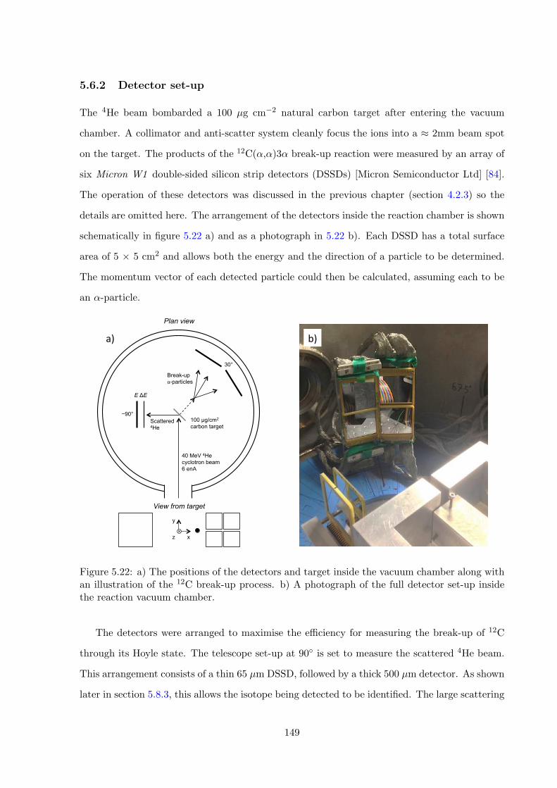
5.6.2 Detector set-up

The 4He beam bombarded a 100 µg cm�2 natural carbon target after entering the vacuum

chamber. A collimator and anti-scatter system cleanly focus the ions into a ⇡ 2mm beam spot

on the target. The products of the 12C(↵,↵)3↵ break-up reaction were measured by an array of

six Micron W1 double-sided silicon strip detectors (DSSDs) [Micron Semiconductor Ltd] [84].

The operation of these detectors was discussed in the previous chapter (section 4.2.3) so the

details are omitted here. The arrangement of the detectors inside the reaction chamber is shown

schematically in figure 5.22 a) and as a photograph in 5.22 b). Each DSSD has a total surface

area of 5 ⇥ 5 cm2 and allows both the energy and the direction of a particle to be determined.

The momentum vector of each detected particle could then be calculated, assuming each to be

an ↵-particle.

]

View from target

Plan view

40 MeV 4He cyclotron beam 6 enA

100 µg/cm2 carbon target

−90°

30°

Break-up α-particles

Scattered 4He

y

x z

E ΔE

a) b)

Figure 5.22: a) The positions of the detectors and target inside the vacuum chamber along withan illustration of the 12C break-up process. b) A photograph of the full detector set-up insidethe reaction vacuum chamber.

The detectors were arranged to maximise the e�ciency for measuring the break-up of 12C

through its Hoyle state. The telescope set-up at 90� is set to measure the scattered 4He beam.

This arrangement consists of a thin 65 µm DSSD, followed by a thick 500 µm detector. As shown

later in section 5.8.3, this allows the isotope being detected to be identified. The large scattering

149

angle ensures that a substantial fraction of the beam momentum is imparted to the recoiling

12C. In the centre-of-mass frame of the decaying 12C, it breaks apart into three ↵-particles with

very low energies, due to the proximity of the Hoyle state to the 3↵ threshold. As the 12C has

a large momentum, these ↵-particles are then boosted into the lab frame to have an average

energy around 6 MeV. The 12C target was rotated by 30� in order to minimise the energy losses

of the break-up ↵-particles before hitting the detectors.

The Quad arrangement of 500 µm DSSDs was positioned to collect all three ↵-particles from

the Hoyle state break-up (complete kinematics). An array of four detectors was chosen for two

reasons. Firstly, four detectors, twice as far from the target provides a superior angular gran-

ularity compared with a single detector closer to the target, since the detector strips subtend

a smaller angular range. Therefore, the momentum of the detected particles can be measured

more accurately.

Secondly, two previous measurements of the direct decay of the Hoyle state noted that,

when measuring multiple particles with similar energies, it was possible to accidentally miss-

assign the hit positions of each particle [138, 140]. Section 4.3 details how, when multiple

particles hit the same detector, the signals collected by the front and rear detector strips are

energy ordered. The signals on the front and rear strips are then matched, and their crossing

point provides the hit position. In cases where the particles have very similar energies, due to

the finite energy resolution of the detectors, it is possible for the energy order of various particles

to be switched. In this case, when the front and back strips are energy ordered and matched,

the extracted strip crossing point is incorrect. This worsens the resolution and provides an

experimental background. Using four separate DSSDs allows for the possibility that each break-

up ↵-particle is detected in a separate DSSD, therefore eliminating this background. In this

experiment, events where two particles strike the same DSSD and events where each particle

strikes a di↵erent DSSD are considered separately. In events where two particles hit the same

DSSD, since the resolutions of the detectors are known, the probability of angular mismatch is

easy to calculate and was incorporated into Monte-Carlo simulations of the reaction.

150

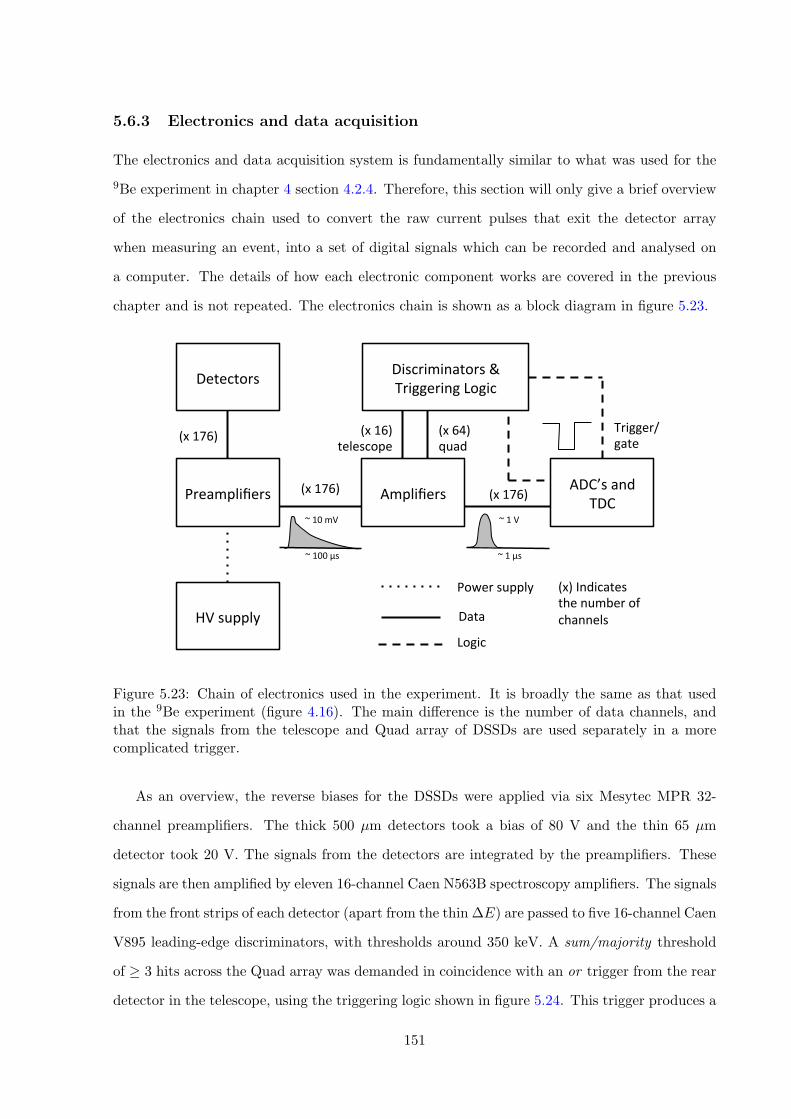
5.6.3 Electronics and data acquisition

The electronics and data acquisition system is fundamentally similar to what was used for the

9Be experiment in chapter 4 section 4.2.4. Therefore, this section will only give a brief overview

of the electronics chain used to convert the raw current pulses that exit the detector array

when measuring an event, into a set of digital signals which can be recorded and analysed on

a computer. The details of how each electronic component works are covered in the previous

chapter and is not repeated. The electronics chain is shown as a block diagram in figure 5.23.

Detectors

Preamplifiers Amplifiers

HVsupply

(x176)

(x176)

(x64)quad

Trigger/gate

Logic

Data

Powersupply (x)Indicatesthenumberofchannels

~10mV

~100μs

~1V

~1μs

(x16)telescope

Discriminators&TriggeringLogic

ADC’sandTDC

(x176)

Figure 5.23: Chain of electronics used in the experiment. It is broadly the same as that usedin the 9Be experiment (figure 4.16). The main di↵erence is the number of data channels, andthat the signals from the telescope and Quad array of DSSDs are used separately in a morecomplicated trigger.

As an overview, the reverse biases for the DSSDs were applied via six Mesytec MPR 32-

channel preamplifiers. The thick 500 µm detectors took a bias of 80 V and the thin 65 µm

detector took 20 V. The signals from the detectors are integrated by the preamplifiers. These

signals are then amplified by eleven 16-channel Caen N563B spectroscopy amplifiers. The signals

from the front strips of each detector (apart from the thin�E) are passed to five 16-channel Caen

V895 leading-edge discriminators, with thresholds around 350 keV. A sum/majority threshold

of � 3 hits across the Quad array was demanded in coincidence with an or trigger from the rear

detector in the telescope, using the triggering logic shown in figure 5.24. This trigger produces a

151

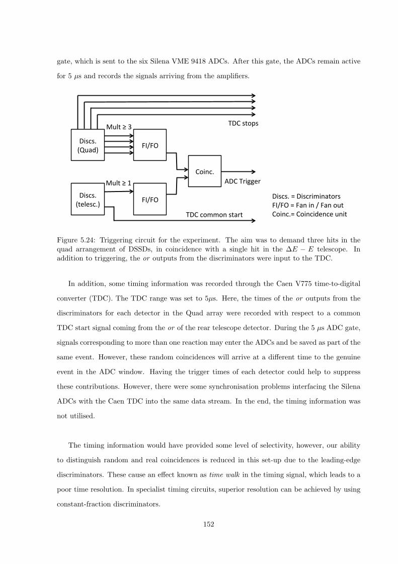
gate, which is sent to the six Silena VME 9418 ADCs. After this gate, the ADCs remain active

for 5 µs and records the signals arriving from the amplifiers.

Discs.(Quad)

Discs.(telesc.)

FI/FO

FI/FO

Coinc.

Mult≥3

Mult≥1

Discs.=DiscriminatorsFI/FO=Fanin/FanoutCoinc.=Coincidenceunit

ADCTrigger

TDCcommonstart

TDCstops

Figure 5.24: Triggering circuit for the experiment. The aim was to demand three hits in thequad arrangement of DSSDs, in coincidence with a single hit in the �E � E telescope. Inaddition to triggering, the or outputs from the discriminators were input to the TDC.

In addition, some timing information was recorded through the Caen V775 time-to-digital

converter (TDC). The TDC range was set to 5µs. Here, the times of the or outputs from the

discriminators for each detector in the Quad array were recorded with respect to a common

TDC start signal coming from the or of the rear telescope detector. During the 5 µs ADC gate,

signals corresponding to more than one reaction may enter the ADCs and be saved as part of the

same event. However, these random coincidences will arrive at a di↵erent time to the genuine

event in the ADC window. Having the trigger times of each detector could help to suppress

these contributions. However, there were some synchronisation problems interfacing the Silena

ADCs with the Caen TDC into the same data stream. In the end, the timing information was

not utilised.

The timing information would have provided some level of selectivity, however, our ability

to distinguish random and real coincidences is reduced in this set-up due to the leading-edge

discriminators. These cause an e↵ect known as time walk in the timing signal, which leads to a

poor time resolution. In specialist timing circuits, superior resolution can be achieved by using

constant-fraction discriminators.

152

5.7 Monte-Carlo simulations

As was seen in chapter 4, Monte-Carlo simulations are essential for a quantitative analysis

of experimental results, and to compare with theoretical predictions. In the case of the 9Be

experiment, Monte-Carlo simulations were used to determine the experimental e�ciency and

resolution as a function of 9Be excitation energy. In this study, the experimental data were

compared to the results of Monte-Carlo simulations of the break-up reaction, in order to extract

the direct 3↵ decay branching ratio. Therefore, it was important to ensure that the simulations

are an accurate reflection of the experiment. Hence, at each stage of the data analysis, the

experimental data are compared with the Monte-Carlo-generated events, in order to check for

consistency. For these reasons, an initial discussion of the Monte-Carlo simulations is useful.

The simulations detailed in this chapter are structured into three parts as follows.

Firstly, the physical reaction process and reaction kinematics are generated. The Monte-

Carlo events were generated using the same code as detailed in section 4.4.1 (references [101,

102]). This code calculates the reaction process as a sequential break-up: a lineage of inde-

pendent two-body decays that lead from the initial to the final state. Therefore, extra sub-

routines were written to generate the various direct decay processes. Beam energy spread and

beam divergence were included when generating 12C(↵,↵)3↵ break-up reactions using this code.

Isotropic angular distributions of the particles were chosen due to the angular momentum of the

reaction of interest, but more complicated anisotropic distributions can be included at this stage.

Secondly, due to the unique detector geometry (incompatible with the general Monte-Carlo

code), all generated events were output to a file and the other experimental e↵ects (listed below)

were enforced in a separate sort code. Thirdly, this code was used to analyse the simulated data

in the same way as the experimental data. This way it is subject to the same data reduction

cuts as the experimental data in order to permit a meaningful comparison.

Experimental e↵ects

1. Energy loss of the beam in the target

153

2. Energy losses of the reaction products in the target

3. Angular and energy straggle in the target

4. Angular straggle in the front face of the DSSD telescope

5. Angular granularity of the detector strips

6. Energy resolution of the detectors (see section 5.8.2)

7. Pile-up of hits on the same strip

8. Background due to event mixing

9. Mis-assignment of hit positions when multiple particles hit the same detector

The majority of these e↵ects were included in the simulations detailed in section 4.4.1. Ef-

fects 8 and 9 were not included in any previous simulations but are important when analysing

this data set.

E↵ect 8

E↵ect 8 simulated the background due to event mixing. As mentioned in section 5.6.3, due

to the relatively high 6 enA beam current, particles from two separate reactions may hit the

detector array during the 5 µs window of the ADCs, registering as a single event. This pro-

duces an unavoidable background since it is a limitation of the measurement apparatus. This

could have been reduced to an extent, using the timing of the detections, but this could not

be implemented. It is, therefore, important to correctly include this event mixing e↵ect in the

Monte-Carlo simulations of the measurement process.

It was first necessary to confirm that the background was really due to event mixing. Since

this e↵ect should scale linearly with the beam current, several short experimental runs at varying

beam currents were recorded. The excitation spectra for 12C were measured (see section 5.8.4

later) and the total peak-to-background ratios were recorded as a function of the beam current.

A plot of this is shown in figure 5.25. A clear correlation was observed, indicating that event

mixing plays a significant part in this experimental background. However, extrapolating a linear

154

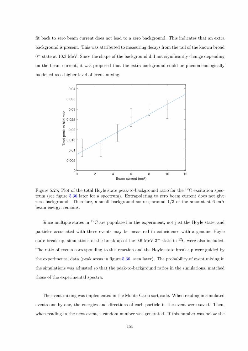
fit back to zero beam current does not lead to a zero background. This indicates that an extra

background is present. This was attributed to measuring decays from the tail of the known broad

0+ state at 10.3 MeV. Since the shape of the background did not significantly change depending

on the beam current, it was proposed that the extra background could be phenomenologically

modelled as a higher level of event mixing.

0 2 4 6 8 10 12Beam current (enA)

0

0.005

0.01

0.015

0.02

0.025

0.03

0.035

0.04

Tota

l pea

k-to

-bkd

ratio

Figure 5.25: Plot of the total Hoyle state peak-to-background ratio for the 12C excitation spec-trum (see figure 5.36 later for a spectrum). Extrapolating to zero beam current does not givezero background. Therefore, a small background source, around 1/3 of the amount at 6 enAbeam energy, remains.

Since multiple states in 12C are populated in the experiment, not just the Hoyle state, and

particles associated with these events may be measured in coincidence with a genuine Hoyle

state break-up, simulations of the break-up of the 9.6 MeV 3� state in 12C were also included.

The ratio of events corresponding to this reaction and the Hoyle state break-up were guided by

the experimental data (peak areas in figure 5.36, seen later). The probability of event mixing in

the simulations was adjusted so that the peak-to-background ratios in the simulations, matched

those of the experimental spectra.

The event mixing was implemented in the Monte-Carlo sort code. When reading in simulated

events one-by-one, the energies and directions of each particle in the event were saved. Then,

when reading in the next event, a random number was generated. If this number was below the

155

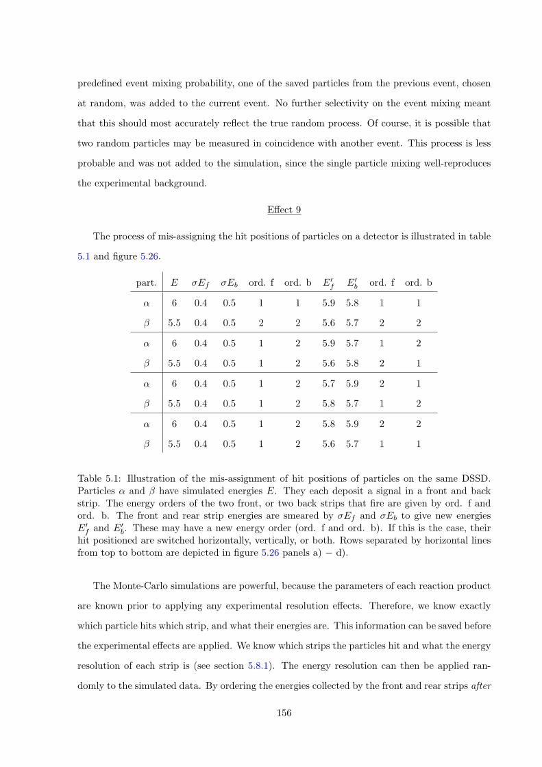
predefined event mixing probability, one of the saved particles from the previous event, chosen

at random, was added to the current event. No further selectivity on the event mixing meant

that this should most accurately reflect the true random process. Of course, it is possible that

two random particles may be measured in coincidence with another event. This process is less

probable and was not added to the simulation, since the single particle mixing well-reproduces

the experimental background.

E↵ect 9

The process of mis-assigning the hit positions of particles on a detector is illustrated in table

5.1 and figure 5.26.

part. E �Ef �Eb ord. f ord. b E0f E0

b ord. f ord. b

↵ 6 0.4 0.5 1 1 5.9 5.8 1 1

� 5.5 0.4 0.5 2 2 5.6 5.7 2 2

↵ 6 0.4 0.5 1 2 5.9 5.7 1 2

� 5.5 0.4 0.5 1 2 5.6 5.8 2 1

↵ 6 0.4 0.5 1 2 5.7 5.9 2 1

� 5.5 0.4 0.5 1 2 5.8 5.7 1 2

↵ 6 0.4 0.5 1 2 5.8 5.9 2 2

� 5.5 0.4 0.5 1 2 5.6 5.7 1 1

Table 5.1: Illustration of the mis-assignment of hit positions of particles on the same DSSD.Particles ↵ and � have simulated energies E. They each deposit a signal in a front and backstrip. The energy orders of the two front, or two back strips that fire are given by ord. f andord. b. The front and rear strip energies are smeared by �Ef and �Eb to give new energiesE0

f and E0b. These may have a new energy order (ord. f and ord. b). If this is the case, their

hit positioned are switched horizontally, vertically, or both. Rows separated by horizontal linesfrom top to bottom are depicted in figure 5.26 panels a) � d).

The Monte-Carlo simulations are powerful, because the parameters of each reaction product

are known prior to applying any experimental resolution e↵ects. Therefore, we know exactly

which particle hits which strip, and what their energies are. This information can be saved before

the experimental e↵ects are applied. We know which strips the particles hit and what the energy

resolution of each strip is (see section 5.8.1). The energy resolution can then be applied ran-

domly to the simulated data. By ordering the energies collected by the front and rear strips after

156

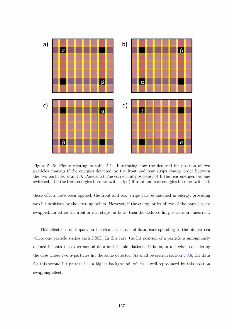
α

β

β

α

α

β

β

α

a) b)

c) d)

Figure 5.26: Figure relating to table 5.1. Illustrating how the deduced hit position of twoparticles changes if the energies detected by the front and rear strips change order betweenthe two particles, ↵ and �. Panels: a) The correct hit positions; b) If the rear energies becomeswitched; c) if the front energies become switched; d) If front and rear energies become switched.

these e↵ects have been applied, the front and rear strips can be matched in energy, providing

two hit positions by the crossing points. However, if the energy order of two of the particles are

swapped, for either the front or rear strips, or both, then the deduced hit positions are incorrect.

This e↵ect has no impact on the cleanest subset of data, corresponding to the hit pattern

where one particle strikes each DSSD. In this case, the hit position of a particle is ambiguously

defined in both the experimental data and the simulations. It is important when considering

the case where two ↵-particles hit the same detector. As shall be seen in section 5.8.6, the data

for this second hit pattern has a higher background, which is well-reproduced by this position

swapping e↵ect.

157

5.8 Primary analysis and data reduction

The data recorded during the beam run were analysed within the SUNSORT framework [93]

using Fortran sort codes. The aim of the primary data analysis stage is to convert the raw data

recorded during the beam run into the various spectra for the 12C nucleus, allowing as little

experimental background through to these spectra as possible.

For this experiment the primary analysis can be separated into several stages. Firstly, a

calibration of the detectors is required in order to convert the ADC values into energies and

to verify the measured positions of the detectors. The experimental energy resolution of the

detectors was then determined. The remainder of the primary analysis can be separated into

several event filtering and calculation steps that shall be described in more detail throughout

the following sections.

158

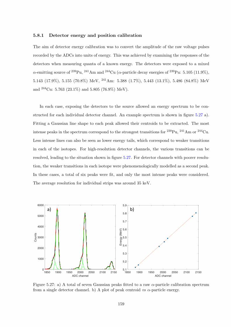
5.8.1 Detector energy and position calibration

The aim of detector energy calibration was to convert the amplitude of the raw voltage pulses

recorded by the ADCs into units of energy. This was achieved by examining the responses of the

detectors when measuring quanta of a known energy. The detectors were exposed to a mixed

↵-emitting source of 239Pu, 241Am and 244Cu (↵-particle decay energies of 239Pu: 5.105 (11.9%),

5.143 (17.9%), 5.155 (70.8%) MeV, 241Am: 5.388 (1.7%), 5.443 (13.1%), 5.486 (84.8%) MeV

and 244Cu: 5.763 (23.1%) and 5.805 (76.9%) MeV).

In each case, exposing the detectors to the source allowed an energy spectrum to be con-

structed for each individual detector channel. An example spectrum is shown in figure 5.27 a).

Fitting a Gaussian line shape to each peak allowed their centroids to be extracted. The most

intense peaks in the spectrum correspond to the strongest transitions for 239Pu, 241Am or 244Cu.

Less intense lines can also be seen as lower energy tails, which correspond to weaker transitions

in each of the isotopes. For high-resolution detector channels, the various transitions can be

resolved, leading to the situation shown in figure 5.27. For detector channels with poorer resolu-

tion, the weaker transitions in each isotope were phenomenologically modelled as a second peak.

In these cases, a total of six peaks were fit, and only the most intense peaks were considered.

The average resolution for individual strips was around 35 keV.

1850 1900 1950 2000 2050 2100 2150ADC channel

0

1000

2000

3000

4000

5000

6000

Cou

nts

1850 1900 1950 2000 2050 2100 2150ADC channel

5.1

5.2

5.3

5.4

5.5

5.6

5.7

5.8

5.9

Ener

gy (M

eV)

a) b)

Figure 5.27: a) A total of seven Gaussian peaks fitted to a raw ↵-particle calibration spectrumfrom a single detector channel. b) A plot of peak centroid vs ↵-particle energy.

159

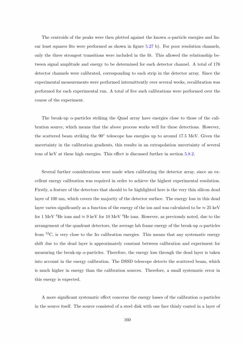
The centroids of the peaks were then plotted against the known ↵-particle energies and lin-

ear least squares fits were performed as shown in figure 5.27 b). For poor resolution channels,

only the three strongest transitions were included in the fit. This allowed the relationship be-

tween signal amplitude and energy to be determined for each detector channel. A total of 176

detector channels were calibrated, corresponding to each strip in the detector array. Since the

experimental measurements were performed intermittently over several weeks, recalibration was

performed for each experimental run. A total of five such calibrations were performed over the

course of the experiment.

The break-up ↵-particles striking the Quad array have energies close to those of the cali-

bration source, which means that the above process works well for these detections. However,

the scattered beam striking the 90� telescope has energies up to around 17.5 MeV. Given the

uncertainty in the calibration gradients, this results in an extrapolation uncertainty of several

tens of keV at these high energies. This e↵ect is discussed further in section 5.8.2.

Several further considerations were made when calibrating the detector array, since an ex-

cellent energy calibration was required in order to achieve the highest experimental resolution.

Firstly, a feature of the detectors that should to be highlighted here is the very thin silicon dead

layer of 100 nm, which covers the majority of the detector surface. The energy loss in this dead

layer varies significantly as a function of the energy of the ion and was calculated to be ⇡ 25 keV

for 1 MeV 4He ions and ⇡ 9 keV for 10 MeV 4He ions. However, as previously noted, due to the

arrangement of the quadrant detectors, the average lab frame energy of the break-up ↵-particles

from 12C, is very close to the 3↵ calibration energies. This means that any systematic energy

shift due to the dead layer is approximately constant between calibration and experiment for

measuring the break-up ↵-particles. Therefore, the energy loss through the dead layer is taken

into account in the energy calibration. The DSSD telescope detects the scattered beam, which

is much higher in energy than the calibration sources. Therefore, a small systematic error in

this energy is expected.

A more significant systematic e↵ect concerns the energy losses of the calibration ↵-particles

in the source itself. The source consisted of a steel disk with one face thinly coated in a layer of

160

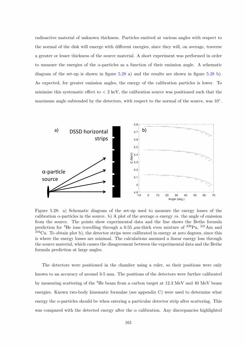
radioactive material of unknown thickness. Particles emitted at various angles with respect to

the normal of the disk will emerge with di↵erent energies, since they will, on average, traverse

a greater or lesser thickness of the source material. A short experiment was performed in order

to measure the energies of the ↵-particles as a function of their emission angle. A schematic

diagram of the set-up is shown in figure 5.28 a) and the results are shown in figure 5.28 b).

As expected, for greater emission angles, the energy of the calibration particles is lower. To

minimise this systematic e↵ect to < 2 keV, the calibration source was positioned such that the

maximum angle subtended by the detectors, with respect to the normal of the source, was 10�.

-10 0 10 20 30 40 50 60 70Angle (deg.)

4.9

5

5.1

5.2

5.3

5.4

5.5

5.6

5.7

5.8

E (M

eV)

DSSDhorizontalstrips

α-par0clesource

a) b)

Figure 5.28: a) Schematic diagram of the set-up used to measure the energy losses of thecalibration ↵-particles in the source. b) A plot of the average ↵ energy vs. the angle of emissionfrom the source. The points show experimental data and the line shows the Bethe formulaprediction for 4He ions travelling through a 0.55 µm-thick even mixture of 239Pu, 241Am and244Cu. To obtain plot b), the detector strips were calibrated in energy at zero degrees, since thisis where the energy losses are minimal. The calculations assumed a linear energy loss throughthe source material, which causes the disagreement between the experimental data and the Betheformula prediction at large angles.

The detectors were positioned in the chamber using a ruler, so their positions were only

known to an accuracy of around 3-5 mm. The positions of the detectors were further calibrated

by measuring scattering of the 4He beam from a carbon target at 12.3 MeV and 40 MeV beam

energies. Known two-body kinematic formulae (see appendix C) were used to determine what

energy the ↵-particles should be when entering a particular detector strip after scattering. This

was compared with the detected energy after the ↵ calibration. Any discrepancies highlighted

161

systematic errors such as slightly incorrect detector positions and angles and allowed for their

correction in the analysis code. Only minor corrections were required. The energies of the

detected ↵-particles as a function of their total scattering angle are shown in figure 5.29.

12750880001800002069810369

5923410631792382187615001090

825612429309218155106

7858463216

86543210

0.0

5.0

10.0

15.0

20.0

25.0

−100.0 −50.0 0.0 50.0 100.0

Ener

gy (M

eV)

Angle (Degrees)

12750880001800002069810369

5923410631792382187615001090

825612429309218155106

7858463216

86543210

0.0

5.0

10.0

15.0

20.0

25.0

−100.0 −50.0 0.0 50.0 100.0

Ener

gy (M

eV)

Angle (Degrees)

Angle(deg.)

Energy(M

eV)

Figure 5.29: The energies the scattered ↵-particles as a function of their angles for a beam energyof 12.3 MeV. The position of the telescope was calibrated with a 40 MeV beam energy and theQuad array was calibrated with a 12.3 MeV beam energy. The positions of the detectors wereslightly adjusted so that the kinematic predictions (black lines) best overlaid the experimentalkinematic lines. The calculated kinematic lines correspond to populating the recoiling 12C in itsground state, 4.4 MeV 2+ state and 7.65 MeV 0+ Hoyle state.

Summary

Using a mixed ↵-emitting source, each detector channel was calibrated in energy. The source

was positioned a su�cient distance away from the detectors such that the energy losses of the

↵-particles in the source itself were minimised. The average resolution for individual strips

was determined to be around 35 keV. When accurately calibrated in energy, the energies of a

scattered beam of ↵-particles were analysed as a function of their scattering angle. This allowed

any small discrepancies in the measured detector positions to be corrected.

162

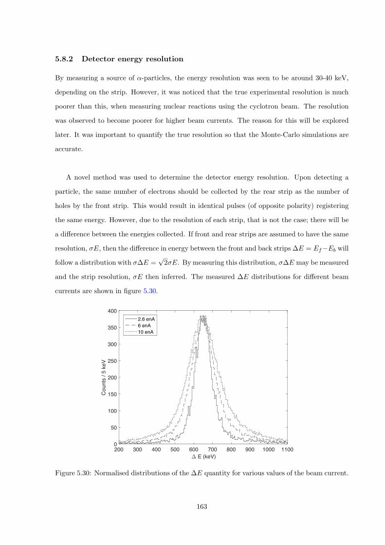
5.8.2 Detector energy resolution

By measuring a source of ↵-particles, the energy resolution was seen to be around 30-40 keV,

depending on the strip. However, it was noticed that the true experimental resolution is much

poorer than this, when measuring nuclear reactions using the cyclotron beam. The resolution

was observed to become poorer for higher beam currents. The reason for this will be explored

later. It was important to quantify the true resolution so that the Monte-Carlo simulations are

accurate.

A novel method was used to determine the detector energy resolution. Upon detecting a

particle, the same number of electrons should be collected by the rear strip as the number of

holes by the front strip. This would result in identical pulses (of opposite polarity) registering

the same energy. However, due to the resolution of each strip, that is not the case; there will be

a di↵erence between the energies collected. If front and rear strips are assumed to have the same

resolution, �E, then the di↵erence in energy between the front and back strips�E = Ef�Eb will

follow a distribution with ��E =p2�E. By measuring this distribution, ��E may be measured

and the strip resolution, �E then inferred. The measured �E distributions for di↵erent beam

currents are shown in figure 5.30.

200 300 400 500 600 700 800 900 1000 1100� E (keV)

0

50

100

150

200

250

300

350

400

Cou

nts

/ 5 k

eV

2.6 enA6 enA10 enA

Figure 5.30: Normalised distributions of the �E quantity for various values of the beam current.

163

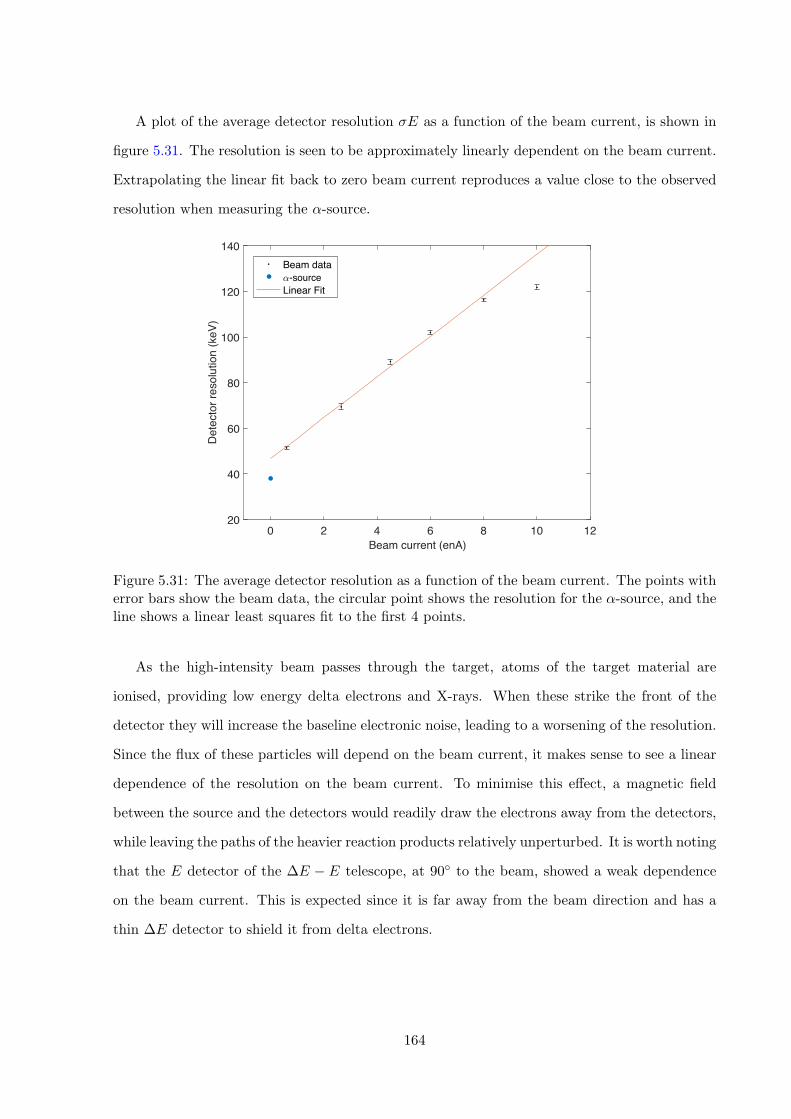
A plot of the average detector resolution �E as a function of the beam current, is shown in

figure 5.31. The resolution is seen to be approximately linearly dependent on the beam current.

Extrapolating the linear fit back to zero beam current reproduces a value close to the observed

resolution when measuring the ↵-source.

0 2 4 6 8 10 12Beam current (enA)

20

40

60

80

100

120

140

Det

ecto

r res

olut

ion

(keV

)

Beam data�-sourceLinear Fit

Figure 5.31: The average detector resolution as a function of the beam current. The points witherror bars show the beam data, the circular point shows the resolution for the ↵-source, and theline shows a linear least squares fit to the first 4 points.

As the high-intensity beam passes through the target, atoms of the target material are

ionised, providing low energy delta electrons and X-rays. When these strike the front of the

detector they will increase the baseline electronic noise, leading to a worsening of the resolution.

Since the flux of these particles will depend on the beam current, it makes sense to see a linear

dependence of the resolution on the beam current. To minimise this e↵ect, a magnetic field

between the source and the detectors would readily draw the electrons away from the detectors,

while leaving the paths of the heavier reaction products relatively unperturbed. It is worth noting

that the E detector of the �E � E telescope, at 90� to the beam, showed a weak dependence

on the beam current. This is expected since it is far away from the beam direction and has a

thin �E detector to shield it from delta electrons.

164

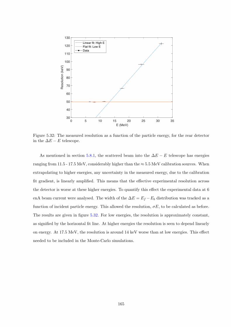
0 5 10 15 20 25 30 35E (MeV)

30

40

50

60

70

80

90

100

110

120

130

Res

olut

ion

(keV

)

Linear fit: High EFlat fit: Low EData

Figure 5.32: The measured resolution as a function of the particle energy, for the rear detectorin the �E � E telescope.

As mentioned in section 5.8.1, the scattered beam into the �E � E telescope has energies

ranging from 11.5 - 17.5 MeV, considerably higher than the⇡ 5.5 MeV calibration sources. When

extrapolating to higher energies, any uncertainty in the measured energy, due to the calibration

fit gradient, is linearly amplified. This means that the e↵ective experimental resolution across

the detector is worse at these higher energies. To quantify this e↵ect the experimental data at 6

enA beam current were analysed. The width of the �E = Ef �Eb distribution was tracked as a

function of incident particle energy. This allowed the resolution, �E, to be calculated as before.

The results are given in figure 5.32. For low energies, the resolution is approximately constant,

as signified by the horizontal fit line. At higher energies the resolution is seen to depend linearly

on energy. At 17.5 MeV, the resolution is around 14 keV worse than at low energies. This e↵ect

needed to be included in the Monte-Carlo simulations.

165

Summary

The resolution of the detectors was found to be di↵erent when measuring reactions using a

high intensity beam of particles, compared with when measuring radiation from the ↵-particle

source. This was quantified by measuring the di↵erence in the energy collected by the front

and rear strips when a single particle was detected. The resolution was seen to have a linear

dependence on beam current. This was attributed to the fact that when exposed to the beam,

atoms of the target material are ionised, providing low energy delta electrons and X-rays, which

strike the detectors. Furthermore, the detector energy resolution was seen to worsen linearly

at energies higher than 12 MeV. This is due to the fact that the detectors were calibrated in

energy with points around 5 MeV. Uncertainties in the fit gradient meant that extrapolations to

higher energies may deviate away from their true values in a linear fashion. These e↵ects were

incorporated into the Monte-Carlo simulations of the reaction.

166

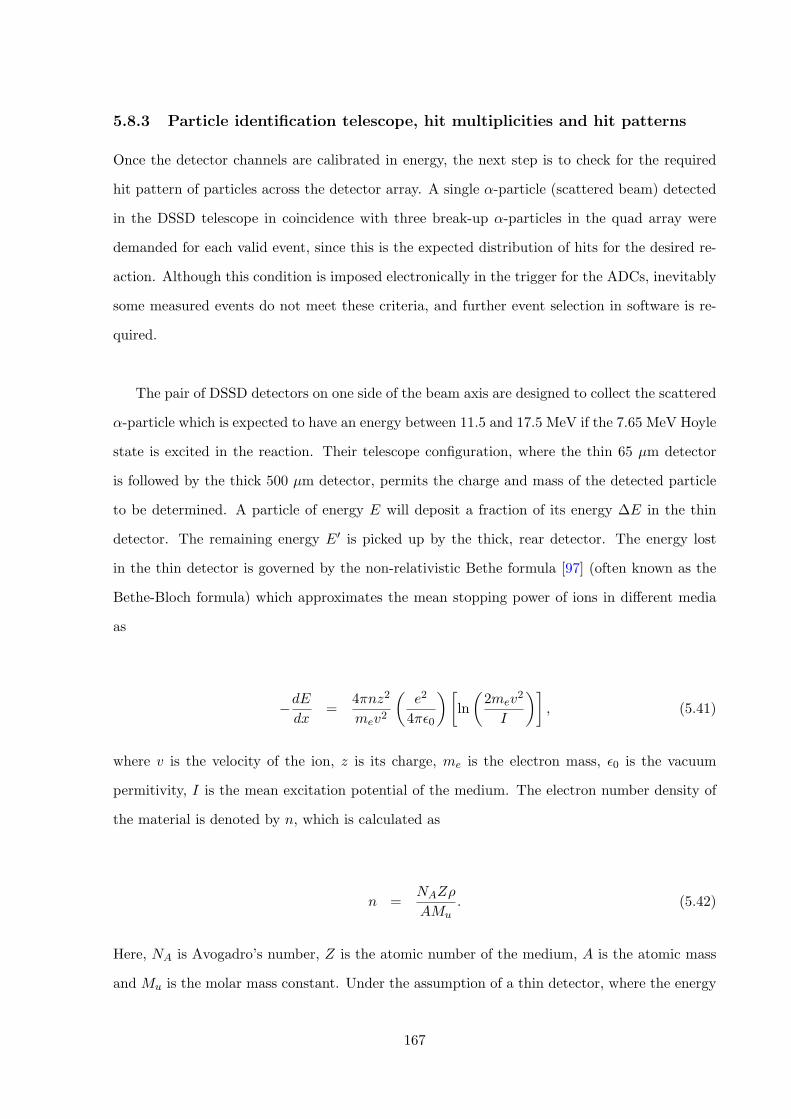
5.8.3 Particle identification telescope, hit multiplicities and hit patterns

Once the detector channels are calibrated in energy, the next step is to check for the required

hit pattern of particles across the detector array. A single ↵-particle (scattered beam) detected

in the DSSD telescope in coincidence with three break-up ↵-particles in the quad array were

demanded for each valid event, since this is the expected distribution of hits for the desired re-

action. Although this condition is imposed electronically in the trigger for the ADCs, inevitably

some measured events do not meet these criteria, and further event selection in software is re-

quired.

The pair of DSSD detectors on one side of the beam axis are designed to collect the scattered

↵-particle which is expected to have an energy between 11.5 and 17.5 MeV if the 7.65 MeV Hoyle

state is excited in the reaction. Their telescope configuration, where the thin 65 µm detector

is followed by the thick 500 µm detector, permits the charge and mass of the detected particle

to be determined. A particle of energy E will deposit a fraction of its energy �E in the thin

detector. The remaining energy E0 is picked up by the thick, rear detector. The energy lost

in the thin detector is governed by the non-relativistic Bethe formula [97] (often known as the

Bethe-Bloch formula) which approximates the mean stopping power of ions in di↵erent media

as

�dE

dx=

4⇡nz2

mev2

✓e2

4⇡✏0

◆ln

✓2mev

2

I

◆�, (5.41)

where v is the velocity of the ion, z is its charge, me is the electron mass, ✏0 is the vacuum

permitivity, I is the mean excitation potential of the medium. The electron number density of

the material is denoted by n, which is calculated as

n =NAZ⇢

AMu. (5.42)

Here, NA is Avogadro’s number, Z is the atomic number of the medium, A is the atomic mass

and Mu is the molar mass constant. Under the assumption of a thin detector, where the energy

167

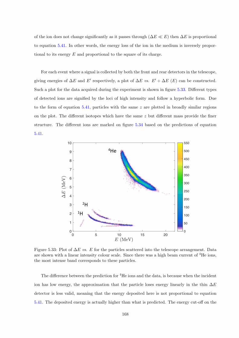
of the ion does not change significantly as it passes through (�E ⌧ E) then �E is proportional

to equation 5.41. In other words, the energy loss of the ion in the medium is inversely propor-

tional to its energy E and proportional to the square of its charge.

For each event where a signal is collected by both the front and rear detectors in the telescope,

giving energies of �E and E0 respectively, a plot of �E vs. E0 +�E (E) can be constructed.

Such a plot for the data acquired during the experiment is shown in figure 5.33. Di↵erent types

of detected ions are signified by the loci of high intensity and follow a hyperbolic form. Due

to the form of equation 5.41, particles with the same z are plotted in broadly similar regions

on the plot. The di↵erent isotopes which have the same z but di↵erent mass provide the finer

structure. The di↵erent ions are marked on figure 5.34 based on the predictions of equation

5.41.

0 5 10 15 20� �����

0

1

2

3

4

5

6

7

8

9

10

��

����

�

0

50

100

150

200

250

300

350

400

450

500

550

1H

2H

4He

Figure 5.33: Plot of �E vs. E for the particles scattered into the telescope arrangement. Dataare shown with a linear intensity colour scale. Since there was a high beam current of 4He ions,the most intense band corresponds to these particles.

The di↵erence between the prediction for 4He ions and the data, is because when the incident

ion has low energy, the approximation that the particle loses energy linearly in the thin �E

detector is less valid, meaning that the energy deposited here is not proportional to equation

5.41. The deposited energy is actually higher than what is predicted. The energy cut-o↵ on the

168

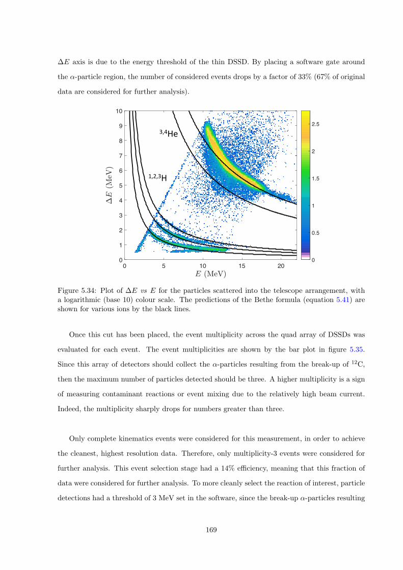
�E axis is due to the energy threshold of the thin DSSD. By placing a software gate around

the ↵-particle region, the number of considered events drops by a factor of 33% (67% of original

data are considered for further analysis).

0 5 10 15 20� �����

0

1

2

3

4

5

6

7

8

9

10�

���

���

0

0.5

1

1.5

2

2.5

1,2,3H

3,4He

Figure 5.34: Plot of �E vs E for the particles scattered into the telescope arrangement, witha logarithmic (base 10) colour scale. The predictions of the Bethe formula (equation 5.41) areshown for various ions by the black lines.

Once this cut has been placed, the event multiplicity across the quad array of DSSDs was

evaluated for each event. The event multiplicities are shown by the bar plot in figure 5.35.

Since this array of detectors should collect the ↵-particles resulting from the break-up of 12C,

then the maximum number of particles detected should be three. A higher multiplicity is a sign

of measuring contaminant reactions or event mixing due to the relatively high beam current.

Indeed, the multiplicity sharply drops for numbers greater than three.

Only complete kinematics events were considered for this measurement, in order to achieve

the cleanest, highest resolution data. Therefore, only multiplicity-3 events were considered for

further analysis. This event selection stage had a 14% e�ciency, meaning that this fraction of

data were considered for further analysis. To more cleanly select the reaction of interest, particle

detections had a threshold of 3 MeV set in the software, since the break-up ↵-particles resulting

169

from the decay of the Hoyle state will have energies greater than this. Up to this point, it is

known from the particle identification telescope that a 4He ion has scattered into the telescope.

It is also known that this was measured in coincidence with three hits across the quad detector

array. The distribution of particles across the detector array is consistent with the inelastic

scattering from 12C and a subsequent break-up into three ↵-particles.

0 1 2 3 4 5 6Multiplicity

0

0.05

0.1

0.15

0.2

0.25

0.3

Frac

tion

of e

vent

s

Figure 5.35: The relative frequencies of hit multiplicities measured across the quad array. Sincethe Hoyle state breaks up into three ↵ particles, the frequency is expected to drop sharplybeyond this multiplicity.

Section 5.6 described that the four DSSDs were chosen to operate within a quadrant geometry

for two reasons. Firstly, four detectors further back from the target provide a superior angular

resolution than a single detector which is closer to the target. Secondly, this geometry permits

each ↵-particle from the 12C break-up to strike a separate DSSD; when two particles with a

similar energy hit the same detector their hit positions may be swapped, leading to an intractable

background. From here in the analysis, the data were split into two categories. The first category

corresponds to the case where each ↵-particle strikes a separate DSSD. The second category

corresponds to where two particles do strike the same DSSD and the third strikes a separate

detector. Of the multiplicity-3 data, 21% occupied category one, and 73% occupied category

two. The remaining 6% of data occupy a third category, where all three ↵-particles hit the same

DSSD. These relative values agree with the results of the Monte-Carlo simulations.

170

Summary

The �E-E telescope arrangement of detectors, designed to collect the scattered ↵-particle beam,

was shown to allow the identification of particles with di↵erent charges, Z, and di↵erent masses,

A. The data follow the relationship predicted by the Bethe-Bloch formula. A software cut

was placed in order to focus on the detected ↵-particles, while ignoring the contributions of

other ions. For these events, the number of particles detected by the quad array of DSSDs was

evaluated. A histogram of the multiplicities showed a sharp drop after a multiplicity of three,

indicating the break-up of 12C into three ↵-particles.

171

5.8.4 Excitation, total energy, and total momentum spectra

Excitation spectra 1

Excitation energy spectra were calculated for the 12C nuclei excited during the reaction. Firstly,

the excitation energies were calculated by using the scattered 4He beam, which was detected

in the telescope configuration. As described in section 4.3.7 for the 9Be experiment, using

momentum conservation between the initial and final states, it was possible to calculate the

momentum of a proposed recoiling nucleus (12C in this case) as

�!P(12C) =

�!Pbeam ��!

P↵. (5.43)

This quantity is calculated from the momentum of the scattered 4He,�!P↵, and the beam only.

Knowing the momentum of the recoiling 12C allows its kinetic energy T (12C) to be calculated.

Using energy conservation, the excitation energy of the proposed recoiling 12C can be calculated

as

Ex = T (12C) + E↵ � Ebeam. (5.44)

The resulting 12C excitation spectrum, corresponding to the subset of data where the break-

up ↵-particles are detected in separate DSSD quadrants, is shown in figure 5.36. The 12C

excitation spectrum, corresponding to when two break-up ↵-particles are detected in the same

DSSD quadrant, is shown in figure 5.37. In both cases, the 0+ Hoyle state at 7.65 MeV is

strongly populated, as is the 3� level at 9.64 MeV. An excitation energy resolution of 570 keV

FWHM was achieved for the Hoyle state. Data within ±2� of the Hoyle state peak centroids

were considered for further analysis. These cuts had an average e�ciency of 56%.

172

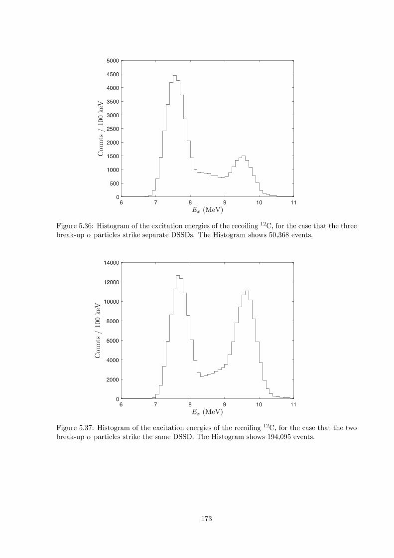
6 7 8 9 10 11�� �����

0

500

1000

1500

2000

2500

3000

3500

4000

4500

5000

���

�

� ��

���

Figure 5.36: Histogram of the excitation energies of the recoiling 12C, for the case that the threebreak-up ↵ particles strike separate DSSDs. The Histogram shows 50,368 events.

6 7 8 9 10 11�� �����

0

2000

4000

6000

8000

10000

12000

14000

���

�

� �

���

�

Figure 5.37: Histogram of the excitation energies of the recoiling 12C, for the case that the twobreak-up ↵ particles strike the same DSSD. The Histogram shows 194,095 events.

173

Total energy spectra

With a cut placed on the excitation energy of 12C, the energies of the particles detected in the

final state were summed. By subtracting the Q-value for the overall 12C(↵,↵)3↵ reaction (�7.27

MeV) from the total 4↵ energy, the beam energy should be calculated.

Figures 5.38 and 5.39 show histograms of the calculated total energies for the experimental

data. Figure 5.38 corresponds to the low-background situation where each ↵-particle from the

12C break-up strikes a separate DSSD in the array. The data corresponding to when two break-

up ↵-particles hit the same DSSD are shown in figure 5.39.

In each plot, the (red) line shows the results of Monte-Carlo simulations of the sequential

decay reaction mechanism. The simulations include experimental resolution e↵ects and event

mixing for background. The peak widths (⇡300 and 350 keV) and the general background shapes

are well-reproduced by the simulations. To minimise background events, only data within ±2�

of the peak centroid were considered for further analysis. This cut had an 85% e�ciency for the

first hit pattern and an e�ciency of 78% for the second hit pattern.

174

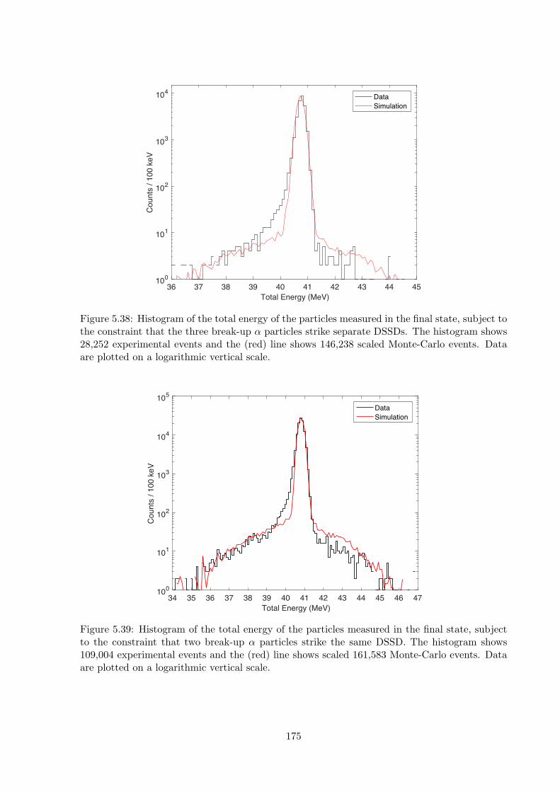
36 37 38 39 40 41 42 43 44 45Total Energy (MeV)

100

101

102

103

104

Cou

nts

/ 100

keV

DataSimulation

Figure 5.38: Histogram of the total energy of the particles measured in the final state, subject tothe constraint that the three break-up ↵ particles strike separate DSSDs. The histogram shows28,252 experimental events and the (red) line shows 146,238 scaled Monte-Carlo events. Dataare plotted on a logarithmic vertical scale.

34 35 36 37 38 39 40 41 42 43 44 45 46 47Total Energy (MeV)

100

101

102

103

104

105

Cou

nts

/ 100

keV

DataSimulation

Figure 5.39: Histogram of the total energy of the particles measured in the final state, subjectto the constraint that two break-up ↵ particles strike the same DSSD. The histogram shows109,004 experimental events and the (red) line shows scaled 161,583 Monte-Carlo events. Dataare plotted on a logarithmic vertical scale.

175

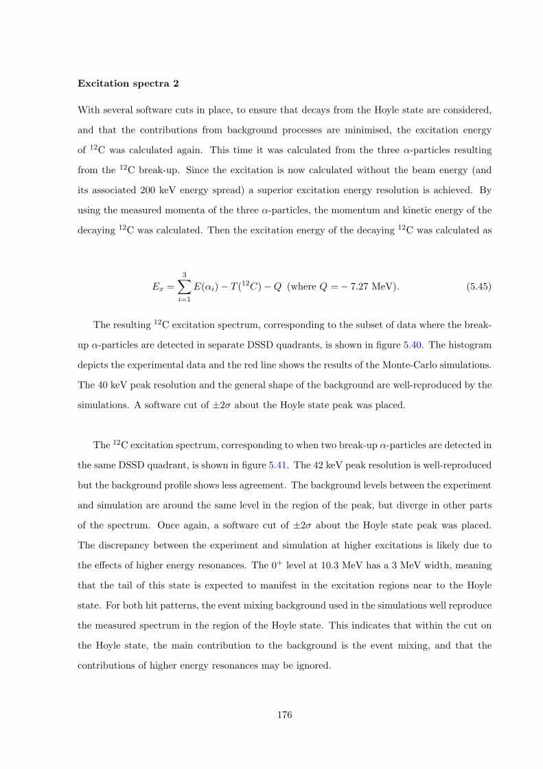
Excitation spectra 2

With several software cuts in place, to ensure that decays from the Hoyle state are considered,

and that the contributions from background processes are minimised, the excitation energy

of 12C was calculated again. This time it was calculated from the three ↵-particles resulting

from the 12C break-up. Since the excitation is now calculated without the beam energy (and

its associated 200 keV energy spread) a superior excitation energy resolution is achieved. By

using the measured momenta of the three ↵-particles, the momentum and kinetic energy of the

decaying 12C was calculated. Then the excitation energy of the decaying 12C was calculated as

Ex =3X

i=1

E(↵i)� T (12C)�Q (where Q =� 7.27 MeV). (5.45)

The resulting 12C excitation spectrum, corresponding to the subset of data where the break-

up ↵-particles are detected in separate DSSD quadrants, is shown in figure 5.40. The histogram

depicts the experimental data and the red line shows the results of the Monte-Carlo simulations.

The 40 keV peak resolution and the general shape of the background are well-reproduced by the

simulations. A software cut of ±2� about the Hoyle state peak was placed.

The 12C excitation spectrum, corresponding to when two break-up ↵-particles are detected in

the same DSSD quadrant, is shown in figure 5.41. The 42 keV peak resolution is well-reproduced

but the background profile shows less agreement. The background levels between the experiment

and simulation are around the same level in the region of the peak, but diverge in other parts

of the spectrum. Once again, a software cut of ±2� about the Hoyle state peak was placed.

The discrepancy between the experiment and simulation at higher excitations is likely due to

the e↵ects of higher energy resonances. The 0+ level at 10.3 MeV has a 3 MeV width, meaning

that the tail of this state is expected to manifest in the excitation regions near to the Hoyle

state. For both hit patterns, the event mixing background used in the simulations well reproduce

the measured spectrum in the region of the Hoyle state. This indicates that within the cut on

the Hoyle state, the main contribution to the background is the event mixing, and that the

contributions of higher energy resonances may be ignored.

176

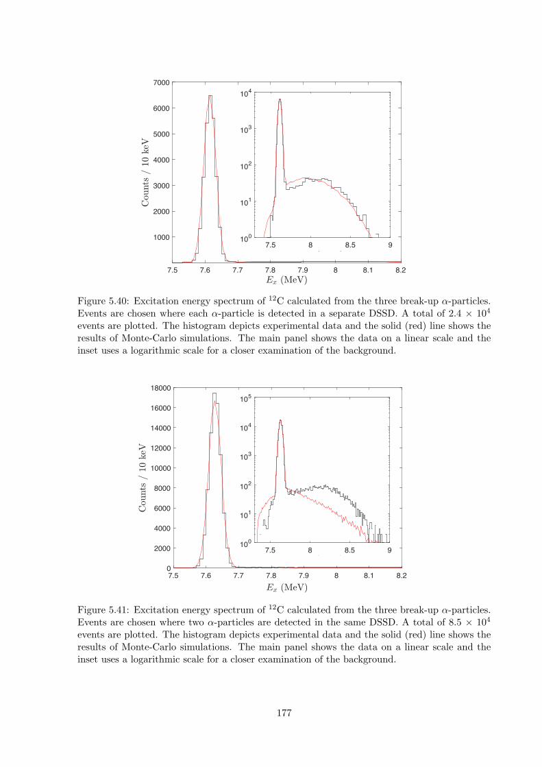
7.5 7.6 7.7 7.8 7.9 8 8.1 8.2�� �����

1000

2000

3000

4000

5000

6000

7000

���

�

� �

���

7.5 8 8.5 9�� �����

100

101

102

103

104

����

� �

���

Figure 5.40: Excitation energy spectrum of 12C calculated from the three break-up ↵-particles.Events are chosen where each ↵-particle is detected in a separate DSSD. A total of 2.4 ⇥ 104

events are plotted. The histogram depicts experimental data and the solid (red) line shows theresults of Monte-Carlo simulations. The main panel shows the data on a linear scale and theinset uses a logarithmic scale for a closer examination of the background.

7.5 7.6 7.7 7.8 7.9 8 8.1 8.2�� �����

0

2000

4000

6000

8000

10000

12000

14000

16000

18000

����

� �

���

7.5 7.6 7.7 7.8 7.9 8 8.1 8.2�� �����

1000

2000

3000

4000

5000

6000

7000

���

�

� �

���

7.5 8 8.5 9�� �����

100

101

102

103

104

105

����

� �

���

Figure 5.41: Excitation energy spectrum of 12C calculated from the three break-up ↵-particles.Events are chosen where two ↵-particles are detected in the same DSSD. A total of 8.5 ⇥ 104

events are plotted. The histogram depicts experimental data and the solid (red) line shows theresults of Monte-Carlo simulations. The main panel shows the data on a linear scale and theinset uses a logarithmic scale for a closer examination of the background.

177

Total momentum spectra

A final software cut was placed on the total momentum of each event in the x, y, z cartesian

directions. The beam direction was chosen to be along the z-axis. This means that in the x

and y directions, the total momenta of the final state particles must sum to zero. In the z di-

rection, the total momentum, minus the beam momentum, should also be zero. For each event,

the momenta in each of these directions were calculated and plotted as a histogram. The data,

corresponding to the case where the three break-up ↵-particles were detected in separate DSSDs

in the array, are plotted in figure 5.42. The data, corresponding to the case when two break-up

↵-particles hit the same DSSD are plotted in figure 5.43. The z-direction plot is shifted by the

initial beam momentum for ease of comparing the three distributions. Only data that simulta-

neously lie within ±2� of each of these peak centroids were considered for further analysis. The

peak centres are o↵set slightly from zero, which is where they expected to be found. This small

systematic shift is a result of an imperfect measurement of the positions of the detectors.

Due to the number of software cuts in place, the data are very clean, and mostly consist of

Hoyle state break-up events. However, despite this, a total of 20 counts can be seen outside of the

main body of these peaks for hit pattern 1 in figure 5.42. Significantly more points can be seen

beyond the tails of the peaks for hit pattern 2 in figure 5.43. This is due to the mis-assignment

of the hit positions when two particles strike the same DSSD. Since the direct break-up process

has such a small branching fraction, these counts are significant, and it is important that they

are factored when calculating any branching ratio. Placing ±2� software cuts on the momentum

peaks provides a way to minimise this background, however, some background exists beneath

the peaks. Assuming that the background is uniform, with four counts in each bin (mean Px

background around the peak), around 50 background events are predicted to bypass this cut

into the final spectra.

178

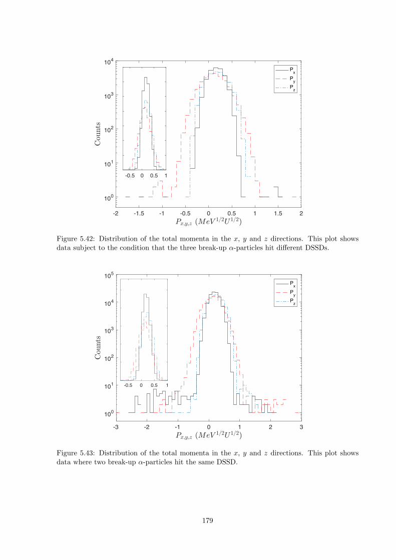
-2 -1.5 -1 -0.5 0 0.5 1 1.5 2������ ���� �� ���

100

101

102

103

104

����

PxPyPz

-0.5 0 0.5 1����� ��� �����

1000

2000

3000

4000

5000

6000

7000

���

Figure 5.42: Distribution of the total momenta in the x, y and z directions. This plot showsdata subject to the condition that the three break-up ↵-particles hit di↵erent DSSDs.

-3 -2 -1 0 1 2 3������ ���� �� ���

100

101

102

103

104

105

����

PxPyPz

-0.5 0 0.5 1������ ���� �� ���

0.5

1

1.5

2

2.5

����

�104

Figure 5.43: Distribution of the total momenta in the x, y and z directions. This plot showsdata where two break-up ↵-particles hit the same DSSD.

179

Summary

The aim of this section of the analysis was to cleanly focus on events corresponding to the

break-up of the 12C Hoyle state into three ↵-particles. Data reduction was achieved in several

ways. Firstly, for each hit pattern, the scattered ↵-particle detected in the �E-E telescope was

used to reconstruct the excitation energy of the recoiling 12C. The 0+ Hoyle state at 7.65 MeV

and 3� state at 9.64 MeV were strongly populated. Software cuts were placed about ±2� of the

Hoyle state peak centroids.

Then, the total energy of each event was calculated, and histograms were plotted. These

total energy spectra, taking into account the break-up Q-value of 12C, peaked at the correct

beam energy. Again, software cuts were placed about ±2� of the total energy peak centroid.

The peak widths and tails of the distribution were well reproduced by Monte-Carlo simulations.

The backgrounds were due to event mixing and mis-match of the hit positions of the particles

on the DSSDs.

Excitation energy spectra were calculated again, this time using the three break-up ↵-

particles detected by the quad array of DSSDs. An excellent energy resolution of 40 keV was

achieved and the small background profiles were well reproduced by the Monte-Carlo simula-

tions. Software cuts were placed about ±2� of the Hoyle state peak centroids.

A final software cut was placed on the total momenta of the detected particles in each of

the cartesian directions. A small amount of data were seen to lie beyond the total momentum

peaks, which were excluded by placing software cuts about ±2� of the peaks.

Monte-Carlo simulations indicated that, after these software cuts were placed, only 0.03%

of background events remained.

180

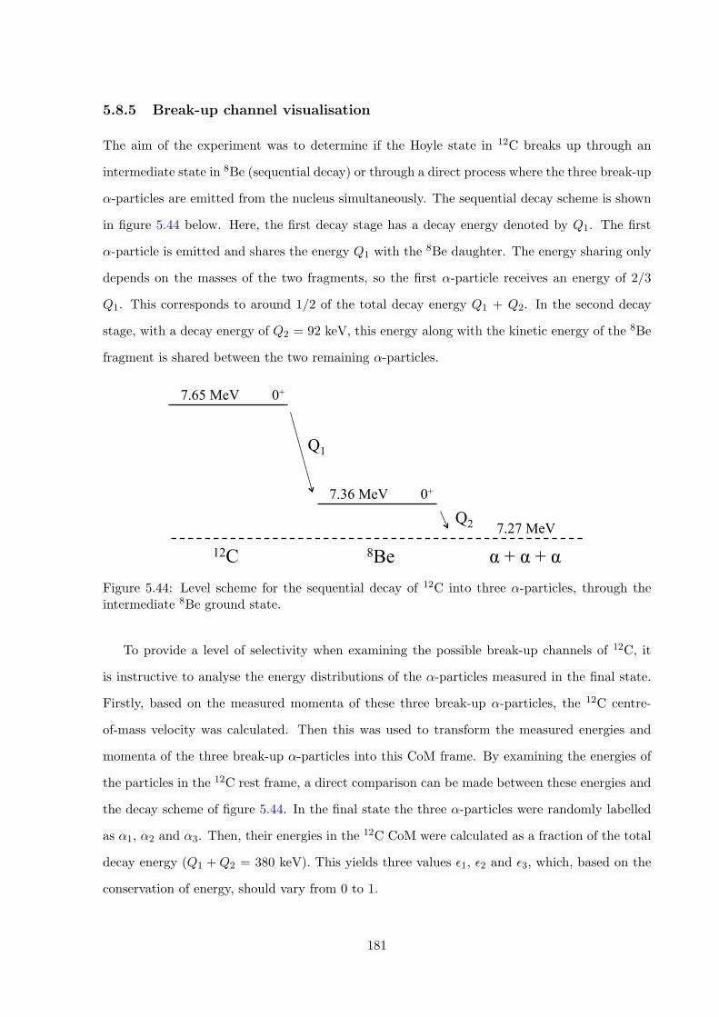
5.8.5 Break-up channel visualisation

The aim of the experiment was to determine if the Hoyle state in 12C breaks up through an

intermediate state in 8Be (sequential decay) or through a direct process where the three break-up

↵-particles are emitted from the nucleus simultaneously. The sequential decay scheme is shown

in figure 5.44 below. Here, the first decay stage has a decay energy denoted by Q1. The first

↵-particle is emitted and shares the energy Q1 with the 8Be daughter. The energy sharing only

depends on the masses of the two fragments, so the first ↵-particle receives an energy of 2/3

Q1. This corresponds to around 1/2 of the total decay energy Q1 + Q2. In the second decay

stage, with a decay energy of Q2 = 92 keV, this energy along with the kinetic energy of the 8Be

fragment is shared between the two remaining ↵-particles.

12C 8Be

7.65 MeV 0+

7.27 MeV

7.36 MeV 0+

Q1

α + α + α

Q2

Figure 5.44: Level scheme for the sequential decay of 12C into three ↵-particles, through theintermediate 8Be ground state.

To provide a level of selectivity when examining the possible break-up channels of 12C, it

is instructive to analyse the energy distributions of the ↵-particles measured in the final state.

Firstly, based on the measured momenta of these three break-up ↵-particles, the 12C centre-

of-mass velocity was calculated. Then this was used to transform the measured energies and

momenta of the three break-up ↵-particles into this CoM frame. By examining the energies of

the particles in the 12C rest frame, a direct comparison can be made between these energies and

the decay scheme of figure 5.44. In the final state the three ↵-particles were randomly labelled

as ↵1, ↵2 and ↵3. Then, their energies in the 12C CoM were calculated as a fraction of the total

decay energy (Q1 +Q2 = 380 keV). This yields three values ✏1, ✏2 and ✏3, which, based on the

conservation of energy, should vary from 0 to 1.

181

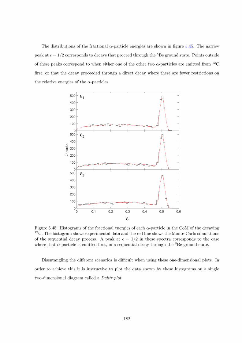
The distributions of the fractional ↵-particle energies are shown in figure 5.45. The narrow

peak at ✏ = 1/2 corresponds to decays that proceed through the 8Be ground state. Points outside

of these peaks correspond to when either one of the other two ↵-particles are emitted from 12C

first, or that the decay proceeded through a direct decay where there are fewer restrictions on

the relative energies of the ↵-particles.

0 0.1 0.2 0.3 0.4 0.5 0.6��

0

100

200

300

400

500

������

0 0.1 0.2 0.3 0.4 0.5 0.6��

0

100

200

300

400

500

������

0 0.1 0.2 0.3 0.4 0.5 0.6��

0

100

200

300

400

500

���

���

ε

ε1

ε2

ε3 0 0.1 0.2 0.3 0.4 0.5 0.6��

0

100

200

300

400

500

���

���

0 0.1 0.2 0.3 0.4 0.5 0.6��

0

100

200

300

400

500

���

���

Figure 5.45: Histograms of the fractional energies of each ↵-particle in the CoM of the decaying12C. The histogram shows experimental data and the red line shows the Monte-Carlo simulationsof the sequential decay process. A peak at ✏ = 1/2 in these spectra corresponds to the casewhere that ↵-particle is emitted first, in a sequential decay through the 8Be ground state.

Disentangling the di↵erent scenarios is di�cult when using these one-dimensional plots. In

order to achieve this it is instructive to plot the data shown by these histograms on a single

two-dimensional diagram called a Dalitz plot.

182

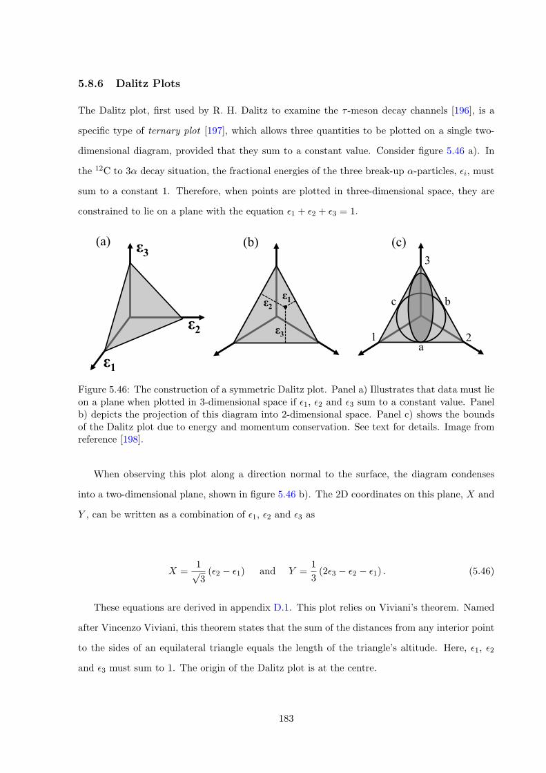
5.8.6 Dalitz Plots

The Dalitz plot, first used by R. H. Dalitz to examine the ⌧ -meson decay channels [196], is a

specific type of ternary plot [197], which allows three quantities to be plotted on a single two-

dimensional diagram, provided that they sum to a constant value. Consider figure 5.46 a). In

the 12C to 3↵ decay situation, the fractional energies of the three break-up ↵-particles, ✏i, must

sum to a constant 1. Therefore, when points are plotted in three-dimensional space, they are

constrained to lie on a plane with the equation ✏1 + ✏2 + ✏3 = 1.

ε1

ε2

ε3

ε2 ε1

ε3 1 2

3

a

b c

(a) (b) (c)

Figure 5.46: The construction of a symmetric Dalitz plot. Panel a) Illustrates that data must lieon a plane when plotted in 3-dimensional space if ✏1, ✏2 and ✏3 sum to a constant value. Panelb) depicts the projection of this diagram into 2-dimensional space. Panel c) shows the boundsof the Dalitz plot due to energy and momentum conservation. See text for details. Image fromreference [198].

When observing this plot along a direction normal to the surface, the diagram condenses

into a two-dimensional plane, shown in figure 5.46 b). The 2D coordinates on this plane, X and

Y , can be written as a combination of ✏1, ✏2 and ✏3 as

X =1p3(✏2 � ✏1) and Y =

1

3(2✏3 � ✏2 � ✏1) . (5.46)

These equations are derived in appendix D.1. This plot relies on Viviani’s theorem. Named

after Vincenzo Viviani, this theorem states that the sum of the distances from any interior point

to the sides of an equilateral triangle equals the length of the triangle’s altitude. Here, ✏1, ✏2

and ✏3 must sum to 1. The origin of the Dalitz plot is at the centre.

183

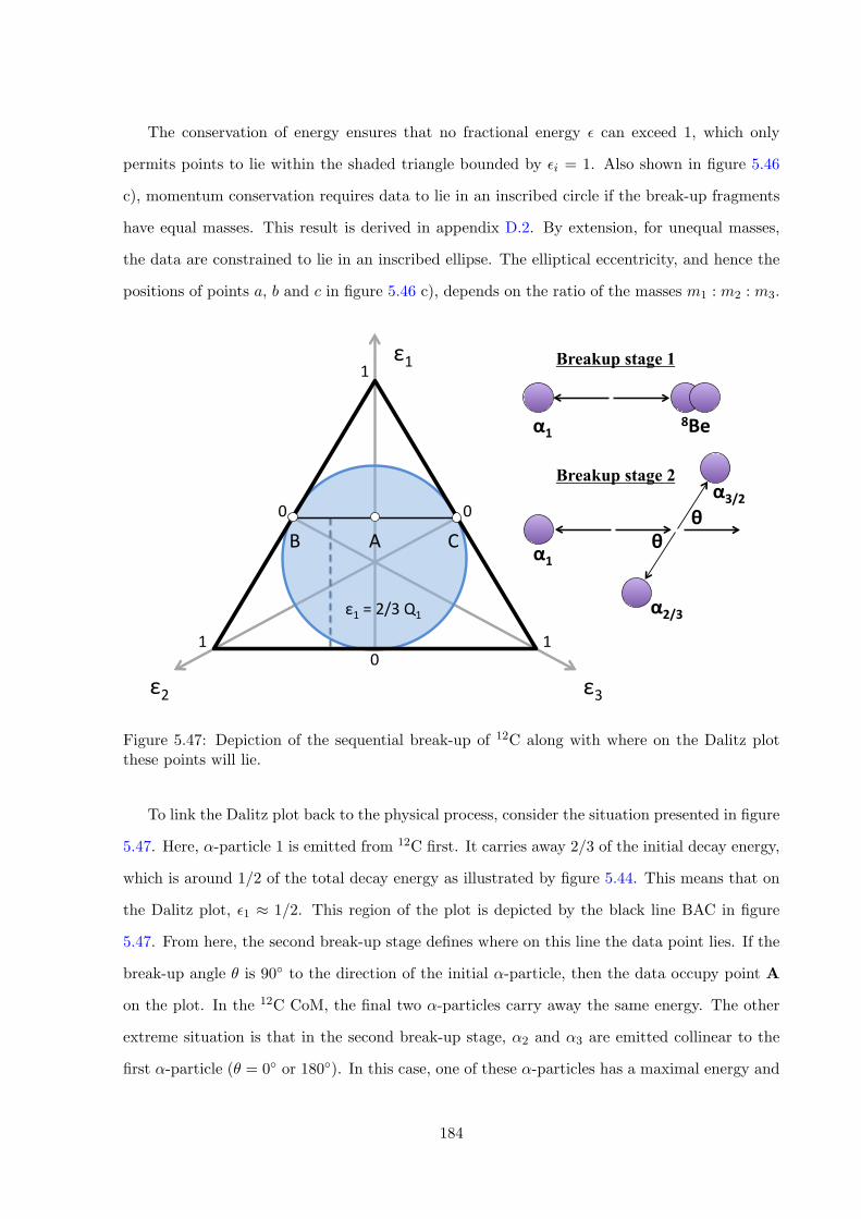
The conservation of energy ensures that no fractional energy ✏ can exceed 1, which only

permits points to lie within the shaded triangle bounded by ✏i = 1. Also shown in figure 5.46

c), momentum conservation requires data to lie in an inscribed circle if the break-up fragments

have equal masses. This result is derived in appendix D.2. By extension, for unequal masses,

the data are constrained to lie in an inscribed ellipse. The elliptical eccentricity, and hence the

positions of points a, b and c in figure 5.46 c), depends on the ratio of the masses m1 : m2 : m3.

ε1

ε3ε2

ε1=2/3Q1

00

011

1

AB C

Breakup stage 1

Breakup stage 2

θθ

α1 8Be

α1

α2/3

α3/2

Figure 5.47: Depiction of the sequential break-up of 12C along with where on the Dalitz plotthese points will lie.

To link the Dalitz plot back to the physical process, consider the situation presented in figure

5.47. Here, ↵-particle 1 is emitted from 12C first. It carries away 2/3 of the initial decay energy,

which is around 1/2 of the total decay energy as illustrated by figure 5.44. This means that on

the Dalitz plot, ✏1 ⇡ 1/2. This region of the plot is depicted by the black line BAC in figure

5.47. From here, the second break-up stage defines where on this line the data point lies. If the

break-up angle ✓ is 90� to the direction of the initial ↵-particle, then the data occupy point A

on the plot. In the 12C CoM, the final two ↵-particles carry away the same energy. The other

extreme situation is that in the second break-up stage, ↵2 and ↵3 are emitted collinear to the

first ↵-particle (✓ = 0� or 180�). In this case, one of these ↵-particles has a maximal energy and

184

the other has zero energy. These correspond to points B and C in figure 5.47. Any collinear

decay occupies the extremities of the Dalitz plot, lying on the edge of the circle. Break-up angles

in the second stage between 0� and 180� occupy the space between B and C.

The width of the black line is due to the natural width of the intermediate state resonance

and the experimental resolution. In cases where the initial state or intermediate resonance

are particularly broad, the e↵ects of varying penetrability through the Coulomb barrier must

be considered when predicting the Dalitz plot distribution. This is achieved through applying

R-matrix theory. Here, both the Hoyle state and intermediate 8Beg.s. are narrow, and so this

e↵ect is ignored. The 8Be ground state ghost anomaly is expected to contribute, but only at

the order of 10�6 compared with the narrow ground state peak [45, 46, 48, 49, 139]. In general,

a variation in intensity along the line is expected due to the angular distributions for the two

break-up stages. In this particular case of Hoyle state (0+) to 8Be (0+) + ↵ (0+) to ↵ + ↵ +

↵ (0+), the angular momentum of the decay is zero meaning isotropic angular distributions are

expected. Therefore, no variation of the intensity across the Dalitz plot is expected.

In the case of general direct break-ups, the three ↵ particles can decay to anywhere in the

available phase space, provided that energy and momentum are conserved. Therefore, points

can lie anywhere inside the blue, shaded circular region of figure 5.47. The point at the very

centre of the Dalitz plot corresponds to the case that each ↵-particle is emitted from the 12C

nucleus with the same energy (✏1 = ✏2 = ✏3 = 1/3) and at angles of 120� to one another. In the

other extreme case, the particles may be emitted collinear to one another, and their energies

may be shared in any way that permits this. These cases would correspond to points on the

very edge of the shaded circle in figure 5.47.

In the experimental analysis, ↵-particles 1, 2 and 3 are assigned randomly, meaning that the

line in figure 5.47 is repeated across the ✏2 and ✏3 axes. Therefore, in the experimental Dalitz

plots, the data occupy triangular loci. As illustrated by figure 5.45, the fractional energies of

each ↵-particle in the CoM of the decaying 12C were calculated. Equations 5.46 were then used

to calculate the Dalitz plot coordinates for each event and a 2D histogram was incremented.

These Dalitz plots are shown in figures 5.48 to 5.50. The Dalitz plots are drawn upside-down

185

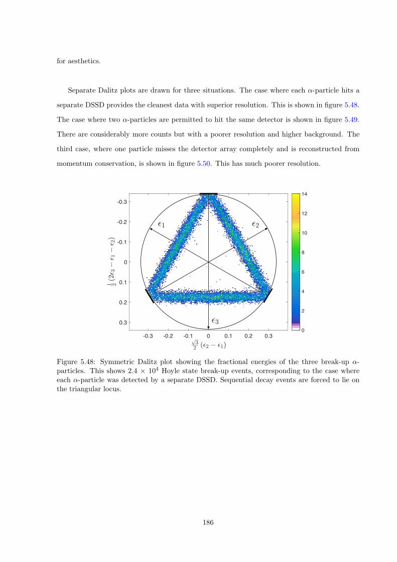
for aesthetics.

Separate Dalitz plots are drawn for three situations. The case where each ↵-particle hits a

separate DSSD provides the cleanest data with superior resolution. This is shown in figure 5.48.

The case where two ↵-particles are permitted to hit the same detector is shown in figure 5.49.

There are considerably more counts but with a poorer resolution and higher background. The

third case, where one particle misses the detector array completely and is reconstructed from

momentum conservation, is shown in figure 5.50. This has much poorer resolution.

-0.3 -0.2 -0.1 0 0.1 0.2 0.3��

� ��� � ���

-0.3

-0.2

-0.1

0

0.1

0.2

0.3

� ���� ��� ��� �

�

0

2

4

6

8

10

12

14

-0.3 -0.2 -0.1 0 0.1 0.2 0.3��

� ��� � ���

-0.3

-0.2

-0.1

0

0.1

0.2

0.3

� ���� ��� ��� �

�

0

2

4

6

8

10

12

14

-0.3 -0.2 -0.1 0 0.1 0.2 0.3��

� ��� � ���

-0.3

-0.2

-0.1

0

0.1

0.2

0.3

� ���� ��� ��� �

�

0

2

4

6

8

10

12

14

-0.3-0.2

-0.10

0.10.2

0.3�

����

���� �

-0.3

-0.2

-0.10

0.1

0.2

0.3

�� ���� � �� � ���

0 2 4 6 8 10 12 14

Figure 5.48: Symmetric Dalitz plot showing the fractional energies of the three break-up ↵-particles. This shows 2.4 ⇥ 104 Hoyle state break-up events, corresponding to the case whereeach ↵-particle was detected by a separate DSSD. Sequential decay events are forced to lie onthe triangular locus.

186

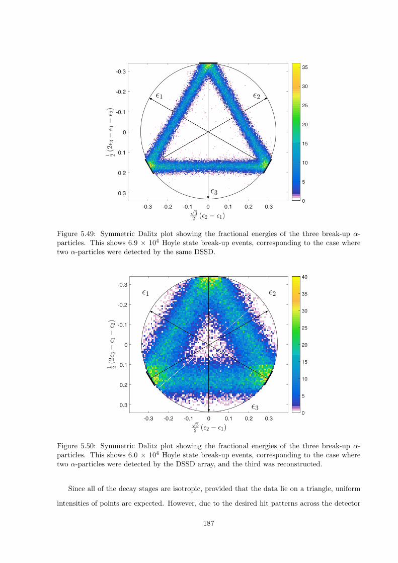
-0.3 -0.2 -0.1 0 0.1 0.2 0.3��

� ��� � ���

-0.3

-0.2

-0.1

0

0.1

0.2

0.3

� ���� ��� ��� �

�

0

2

4

6

8

10

12

14

-0.3 -0.2 -0.1 0 0.1 0.2 0.3��

� ��� � ���

-0.3

-0.2

-0.1

0

0.1

0.2

0.3

� ���� ��� ��� �

�

0

5

10

15

20

25

30

35

-0.3 -0.2 -0.1 0 0.1 0.2 0.3��

� ��� � ���

-0.3

-0.2

-0.1

0

0.1

0.2

0.3

� ���� ��� ��� �

�

0

2

4

6

8

10

12

14

-0.3 -0.2 -0.1 0 0.1 0.2 0.3��

� ��� � ���

-0.3

-0.2

-0.1

0

0.1

0.2

0.3

� ���� ��� ��� �

�

0

2

4

6

8

10

12

14

-0.3-0.2

-0.10

0.10.2

0.3�

����

���� �

-0.3

-0.2

-0.10

0.1

0.2

0.3

�� ���� � �� � ���

0 2 4 6 8 10 12 14

-0.3 -0.2 -0.1 0 0.1 0.2 0.3��

� ��� � ���

-0.3

-0.2

-0.1

0

0.1

0.2

0.3

� ���� ��� ��� �

�

0

2

4

6

8

10

12

14

-0.3 -0.2 -0.1 0 0.1 0.2 0.3��

� ��� � ���

-0.3

-0.2

-0.1

0

0.1

0.2

0.3

� ���� ��� ��� �

�

0

2

4

6

8

10

12

14

-0.3-0.2

-0.10

0.10.2

0.3�

����

���� �

-0.3

-0.2

-0.10

0.1

0.2

0.3

�� ���� � �� � ���

0 2 4 6 8 10 12 14

Figure 5.49: Symmetric Dalitz plot showing the fractional energies of the three break-up ↵-particles. This shows 6.9 ⇥ 104 Hoyle state break-up events, corresponding to the case wheretwo ↵-particles were detected by the same DSSD.

-0.3 -0.2 -0.1 0 0.1 0.2 0.3��

� ��� � ���

-0.3

-0.2

-0.1

0

0.1

0.2

0.3

� ���� ��� ��� �

�

0

2

4

6

8

10

12

14

-0.3 -0.2 -0.1 0 0.1 0.2 0.3��

� ��� � ���

-0.3

-0.2

-0.1

0

0.1

0.2

0.3

� ���� ��� ��� �

�

0

5

10

15

20

25

30

35

40-0.3 -0.2 -0.1 0 0.1 0.2 0.3��

� ��� � ���

-0.3

-0.2

-0.1

0

0.1

0.2

0.3

� ���� ��� ��� �

�

0

2

4

6

8

10

12

14

-0.3 -0.2 -0.1 0 0.1 0.2 0.3��

� ��� � ���

-0.3

-0.2

-0.1

0

0.1

0.2

0.3

� ���� ��� ��� �

�

0

2

4

6

8

10

12

14

-0.3-0.2

-0.10

0.10.2

0.3�

����

���� �

-0.3

-0.2

-0.10

0.1

0.2

0.3

�� ���� � �� � ���

0 2 4 6 8 10 12 14

Figure 5.50: Symmetric Dalitz plot showing the fractional energies of the three break-up ↵-particles. This shows 6.0 ⇥ 104 Hoyle state break-up events, corresponding to the case wheretwo ↵-particles were detected by the DSSD array, and the third was reconstructed.

Since all of the decay stages are isotropic, provided that the data lie on a triangle, uniform

intensities of points are expected. However, due to the desired hit patterns across the detector

187

array, di↵erences in intensities are observed. Events where the particles emerge with similar

energies are more likely to satisfy the requirement that each ↵-particle hits a separate DSSD.

Therefore, a higher intensity of points are observed for regions which lie at smaller radii from the

centre of the Dalitz plot in figure 5.48. Likewise, events which are more collinear are more likely

to satisfy the condition that two ↵-particles hit the same DSSD. Therefore, a higher intensity

of points are seen closer to the edge of the Dalitz plot in figure 5.49.

It is easy to see, most clearly in figures 5.48 and 5.49, that the sequential decay of the Hoyle

state dominates, since most data lie on the triangular loci. Very few points lie in the areas

outside and inside of the triangles, which are expected to be occupied by events originating from

direct decay processes. Any direct decay contribution is small, and in order to quantify this, the

experimental data were compared with Monte-Carlo simulations of sequential and direct decay

processes. To permit a quantitative comparison, figures 5.48 and 5.49 were modified. Due to

the 120� rotational symmetry of the Dalitz plot, it is possible to fold the experimental data

such that a single sextant of the Dalitz plot is occupied. This was achieved through a series of

inversions and rotations of the X and Y Dalitz plot coordinates of each event. The folded data

are shown in figure 5.51.

At this point, it is constructive to compare these figures with those of two previous mea-

surements of the Hoyle state decay, shown in figure 5.52 and from references [139, 140]. In the

present study, a total of 9.3 ⇥ 104 events were measured. The previous two studies measured

around 5 ⇥ 103 and 2 ⇥ 104 events respectively. By comparing figures 5.51 and 5.52, it is clear

that the present measurements have significantly lower backgrounds than previous experiments.

A similar experimental resolution was achieved by each of the experiments, denoted by the width

of the triangle bands. However, references [139, 140] relied on the technique of kinematic fitting

to achieve this resolution. The technique is described later in section 5.8.8 but was not used in

the present analysis. It was found to considerably improve the resolution of the events where

one ↵-particle was reconstructed (figure 5.50), but did not significantly improve the resolution

when applied to complete kinematics events (figures 5.48 and 5.49).

188

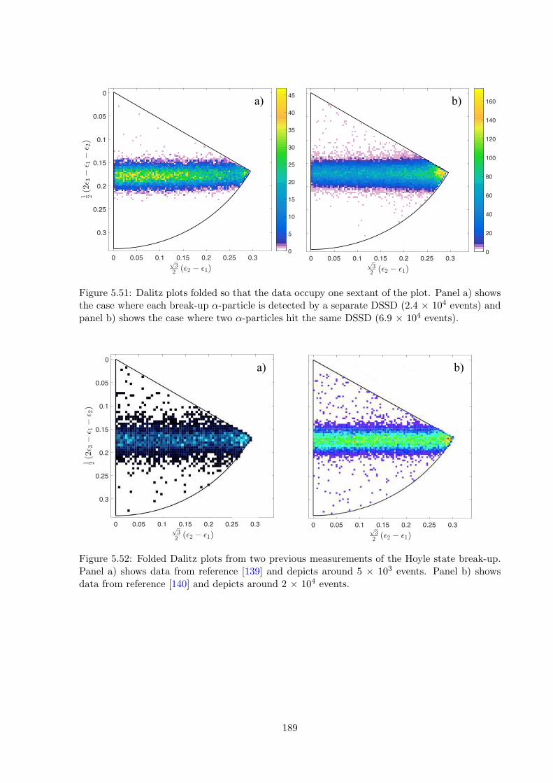
0 0.05 0.1 0.15 0.2 0.25 0.3��

� ��� � ���

0

0.05

0.1

0.15

0.2

0.25

0.3

� ���� ��� ��� �

�

0

20

40

60

80

100

120

140

160

0 0.05 0.1 0.15 0.2 0.25 0.3��

� ��� � ���

0

0.05

0.1

0.15

0.2

0.25

0.3

� ���� ��� ��� �

�

0

5

10

15

20

25

30

35

40

45a) b)

Figure 5.51: Dalitz plots folded so that the data occupy one sextant of the plot. Panel a) showsthe case where each break-up ↵-particle is detected by a separate DSSD (2.4 ⇥ 104 events) andpanel b) shows the case where two ↵-particles hit the same DSSD (6.9 ⇥ 104 events).

0 0.05 0.1 0.15 0.2 0.25 0.3��

� ��� � ���

0

0.05

0.1

0.15

0.2

0.25

0.3

� ���� ��� ��� �

�

0

20

40

60

80

100

120

140

160

0 0.05 0.1 0.15 0.2 0.25 0.3��

� ��� � ���

0

0.05

0.1

0.15

0.2

0.25

0.3

� ���� ��� ��� �

�

0

5

10

15

20

25

30

35

40

45 b) a)

Figure 5.52: Folded Dalitz plots from two previous measurements of the Hoyle state break-up.Panel a) shows data from reference [139] and depicts around 5 ⇥ 103 events. Panel b) showsdata from reference [140] and depicts around 2 ⇥ 104 events.

189

Summary

The sequential and direct decays of the Hoyle state can be disentangled by examining the relative

energies of each of the three ↵-particles that are emitted during the break-up. This is because,

during the sequential decay, the first emitted ↵-particle has a fixed energy, determined by the

masses of the 8Be and ↵-particle fragments (around 1/2 of the total decay energy). A convenient

way to do this is to plot all three of the energies on a single two-dimensional Dalitz plot. On the

Dalitz plot, sequential decays of the Hoyle state appear as a triangular locus. During a direct

break-up, the decay energy can be shared between the three ↵-particle fragments in a more

complicated way, which appears as a background to this triangle. Due to the 120� rotational

symmetry of the Dalitz plot, it is possible to manipulate the data such that they occupy a single

sextant of the plot. Comparing the resulting plots with those of previous publications indicates

the present experiment has higher statistics and lower background.

190

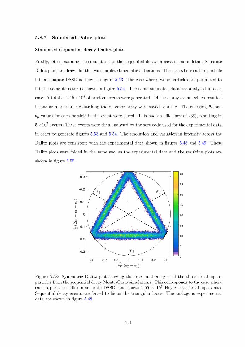
5.8.7 Simulated Dalitz plots

Simulated sequential decay Dalitz plots

Firstly, let us examine the simulations of the sequential decay process in more detail. Separate

Dalitz plots are drawn for the two complete kinematics situations. The case where each ↵-particle

hits a separate DSSD is shown in figure 5.53. The case where two ↵-particles are permitted to

hit the same detector is shown in figure 5.54. The same simulated data are analysed in each

case. A total of 2.15⇥108 of random events were generated. Of these, any events which resulted

in one or more particles striking the detector array were saved to a file. The energies, ✓x and

✓y values for each particle in the event were saved. This had an e�ciency of 23%, resulting in

5⇥107 events. These events were then analysed by the sort code used for the experimental data

in order to generate figures 5.53 and 5.54. The resolution and variation in intensity across the

Dalitz plots are consistent with the experimental data shown in figures 5.48 and 5.49. These

Dalitz plots were folded in the same way as the experimental data and the resulting plots are

shown in figure 5.55.

-0.3 -0.2 -0.1 0 0.1 0.2 0.3��

� ��� � ���

-0.3

-0.2

-0.1

0

0.1

0.2

0.3

� ���� ��� ��� �

�

0

5

10

15

20

25

30

35

40

-0.3 -0.2 -0.1 0 0.1 0.2 0.3��

� ��� � ���

-0.3

-0.2

-0.1

0

0.1

0.2

0.3

� ���� ��� ��� �

�

0

2

4

6

8

10

12

14

-0.3 -0.2 -0.1 0 0.1 0.2 0.3��

� ��� � ���

-0.3

-0.2

-0.1

0

0.1

0.2

0.3

� ���� ��� ��� �

�

0

2

4

6

8

10

12

14

-0.3-0.2

-0.10

0.10.2

0.3�

����

���� �

-0.3

-0.2

-0.10

0.1

0.2

0.3

�� ���� � �� � ���

0 2 4 6 8 10 12 14

-0.3 -0.2 -0.1 0 0.1 0.2 0.3��

� ��� � ���

-0.3

-0.2

-0.1

0

0.1

0.2

0.3

� ���� ��� ��� �

�

0

2

4

6

8

10

12

14

-0.3 -0.2 -0.1 0 0.1 0.2 0.3��

� ��� � ���

-0.3

-0.2

-0.1

0

0.1

0.2

0.3

� ���� ��� ��� �

�

0

2

4

6

8

10

12

14

-0.3-0.2

-0.10

0.10.2

0.3�

����

���� �

-0.3

-0.2

-0.10

0.1

0.2

0.3

�� ���� � �� � ���

0 2 4 6 8 10 12 14

Figure 5.53: Symmetric Dalitz plot showing the fractional energies of the three break-up ↵-particles from the sequential decay Monte-Carlo simulations. This corresponds to the case whereeach ↵-particle strikes a separate DSSD, and shows 1.09 ⇥ 105 Hoyle state break-up events.Sequential decay events are forced to lie on the triangular locus. The analogous experimentaldata are shown in figure 5.48.

191

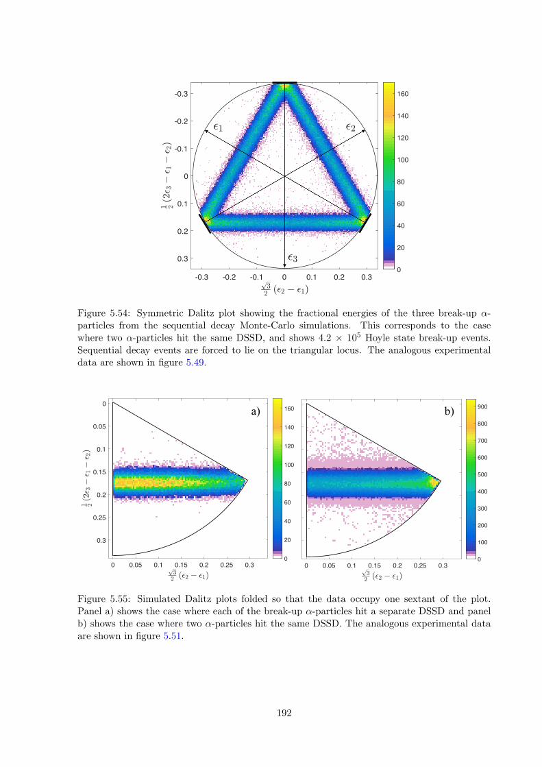
-0.3 -0.2 -0.1 0 0.1 0.2 0.3��

� ��� � ���

-0.3

-0.2

-0.1

0

0.1

0.2

0.3

� ���� ��� ��� �

�

0

20

40

60

80

100

120

140

160

-0.3 -0.2 -0.1 0 0.1 0.2 0.3��

� ��� � ���

-0.3

-0.2

-0.1

0

0.1

0.2

0.3

� ���� ��� ��� �

�

0

2

4

6

8

10

12

14

-0.3 -0.2 -0.1 0 0.1 0.2 0.3��

� ��� � ���

-0.3

-0.2

-0.1

0

0.1

0.2

0.3

� ���� ��� ��� �

�

0

2

4

6

8

10

12

14

-0.3-0.2

-0.10

0.10.2

0.3�

����

���� �

-0.3

-0.2

-0.10

0.1

0.2

0.3

�� ���� � �� � ���

0 2 4 6 8 10 12 14

-0.3 -0.2 -0.1 0 0.1 0.2 0.3��

� ��� � ���

-0.3

-0.2

-0.1

0

0.1

0.2

0.3

� ���� ��� ��� �

�

0

2

4

6

8

10

12

14

-0.3 -0.2 -0.1 0 0.1 0.2 0.3��

� ��� � ���

-0.3

-0.2

-0.1

0

0.1

0.2

0.3

� ���� ��� ��� �

�

0

2

4

6

8

10

12

14

-0.3-0.2

-0.10

0.10.2

0.3�

����

���� �

-0.3

-0.2

-0.10

0.1

0.2

0.3

�� ���� � �� � ���

0 2 4 6 8 10 12 14

Figure 5.54: Symmetric Dalitz plot showing the fractional energies of the three break-up ↵-particles from the sequential decay Monte-Carlo simulations. This corresponds to the casewhere two ↵-particles hit the same DSSD, and shows 4.2 ⇥ 105 Hoyle state break-up events.Sequential decay events are forced to lie on the triangular locus. The analogous experimentaldata are shown in figure 5.49.

0 0.05 0.1 0.15 0.2 0.25 0.3��

� ��� � ���

0

0.05

0.1

0.15

0.2

0.25

0.3

� ���� ��� ��� �

�

0

100

200

300

400

500

600

700

800

900

0 0.05 0.1 0.15 0.2 0.25 0.3��

� ��� � ���

0

0.05

0.1

0.15

0.2

0.25

0.3

� ���� ��� ��� �

�

0

20

40

60

80

100

120

140

160a) b)

Figure 5.55: Simulated Dalitz plots folded so that the data occupy one sextant of the plot.Panel a) shows the case where each of the break-up ↵-particles hit a separate DSSD and panelb) shows the case where two ↵-particles hit the same DSSD. The analogous experimental dataare shown in figure 5.51.

192

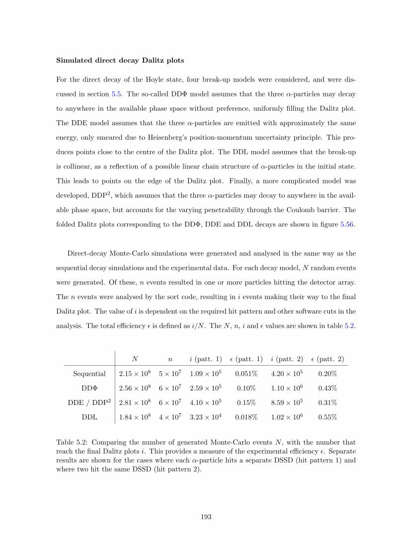
Simulated direct decay Dalitz plots

For the direct decay of the Hoyle state, four break-up models were considered, and were dis-

cussed in section 5.5. The so-called DD� model assumes that the three ↵-particles may decay

to anywhere in the available phase space without preference, uniformly filling the Dalitz plot.

The DDE model assumes that the three ↵-particles are emitted with approximately the same

energy, only smeared due to Heisenberg’s position-momentum uncertainty principle. This pro-

duces points close to the centre of the Dalitz plot. The DDL model assumes that the break-up

is collinear, as a reflection of a possible linear chain structure of ↵-particles in the initial state.

This leads to points on the edge of the Dalitz plot. Finally, a more complicated model was

developed, DDP2, which assumes that the three ↵-particles may decay to anywhere in the avail-

able phase space, but accounts for the varying penetrability through the Coulomb barrier. The

folded Dalitz plots corresponding to the DD�, DDE and DDL decays are shown in figure 5.56.

Direct-decay Monte-Carlo simulations were generated and analysed in the same way as the

sequential decay simulations and the experimental data. For each decay model, N random events

were generated. Of these, n events resulted in one or more particles hitting the detector array.

The n events were analysed by the sort code, resulting in i events making their way to the final

Dalitz plot. The value of i is dependent on the required hit pattern and other software cuts in the

analysis. The total e�ciency ✏ is defined as i/N . The N , n, i and ✏ values are shown in table 5.2.

N n i (patt. 1) ✏ (patt. 1) i (patt. 2) ✏ (patt. 2)

Sequential 2.15⇥ 108 5⇥ 107 1.09⇥ 105 0.051% 4.20⇥ 105 0.20%

DD� 2.56⇥ 108 6⇥ 107 2.59⇥ 105 0.10% 1.10⇥ 106 0.43%

DDE / DDP2 2.81⇥ 108 6⇥ 107 4.10⇥ 105 0.15% 8.59⇥ 105 0.31%

DDL 1.84⇥ 108 4⇥ 107 3.23⇥ 104 0.018% 1.02⇥ 106 0.55%

Table 5.2: Comparing the number of generated Monte-Carlo events N , with the number thatreach the final Dalitz plots i. This provides a measure of the experimental e�ciency ✏. Separateresults are shown for the cases where each ↵-particle hits a separate DSSD (hit pattern 1) andwhere two hit the same DSSD (hit pattern 2).

193

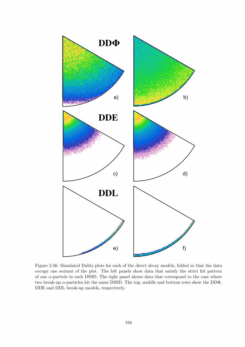
0 0.05 0.1 0.15 0.2 0.25 0.3 0.35��

� ��� � ���

0

0.05

0.1

0.15

0.2

0.25

0.3

0.35

� ���� ��� ��� �

�

0

1000

2000

3000

4000

5000

6000

7000

8000

9000

10000

0 0.05 0.1 0.15 0.2 0.25 0.3 0.35��

� ��� � ���

0

0.05

0.1

0.15

0.2

0.25

0.3

0.35

� ���� ��� ��� �

�

0

100

200

300

400

500

600

700

800

0 0.05 0.1 0.15 0.2 0.25 0.3 0.35��

� ��� � ���

0

0.05

0.1

0.15

0.2

0.25

0.3

0.35

� ���� ��� ��� �

�

0

500

1000

1500

0 0.05 0.1 0.15 0.2 0.25 0.3 0.35��

� ��� � ���

0

0.05

0.1

0.15

0.2

0.25

0.3

0.35

� ���� ��� ��� �

�

0

100

200

300

400

500

600

700

8000 0.05 0.1 0.15 0.2 0.25 0.3 0.35��

� ��� � ���

0

0.05

0.1

0.15

0.2

0.25

0.3

0.35

� ���� ��� ��� �

�

0

20

40

60

80

100

0 0.05 0.1 0.15 0.2 0.25 0.3 0.35��

� ��� � ���

0

0.05

0.1

0.15

0.2

0.25

0.3

0.35

� ���� ��� ��� �

�

0

50

100

150

200

250

300

350

a) b)

c) d)

e) f)

DDΦ

DDE

DDL

Figure 5.56: Simulated Dalitz plots for each of the direct decay models, folded so that the dataoccupy one sextant of the plot. The left panels show data that satisfy the strict hit patternof one ↵-particle in each DSSD. The right panel shows data that correspond to the case wheretwo break-up ↵-particles hit the same DSSD. The top, middle and bottom rows show the DD�,DDE and DDL break-up models, respectively.

194

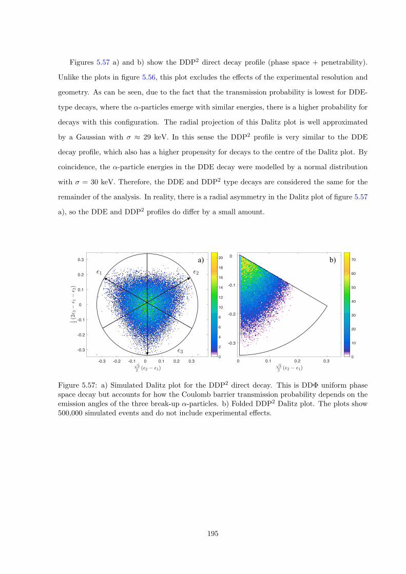
Figures 5.57 a) and b) show the DDP2 direct decay profile (phase space + penetrability).

Unlike the plots in figure 5.56, this plot excludes the e↵ects of the experimental resolution and

geometry. As can be seen, due to the fact that the transmission probability is lowest for DDE-

type decays, where the ↵-particles emerge with similar energies, there is a higher probability for

decays with this configuration. The radial projection of this Dalitz plot is well approximated

by a Gaussian with � ⇡ 29 keV. In this sense the DDP2 profile is very similar to the DDE

decay profile, which also has a higher propensity for decays to the centre of the Dalitz plot. By

coincidence, the ↵-particle energies in the DDE decay were modelled by a normal distribution

with � = 30 keV. Therefore, the DDE and DDP2 type decays are considered the same for the

remainder of the analysis. In reality, there is a radial asymmetry in the Dalitz plot of figure 5.57

a), so the DDE and DDP2 profiles do di↵er by a small amount.

0 0.1 0.2 0.3 ��

� ��� � ���

-0.3

-0.2

-0.1

0

� ���� ��� ��� �

�

0

10

20

30

40

50

60

70

DDP2

b)

-0.3 -0.2 -0.1 0 0.1 0.2 0.3 ��

� ��� � ���

-0.3

-0.2

-0.1

0

0.1

0.2

0.3

� ���� ��� ��� �

�

0

2

4

6

8

10

12

14

16

18

20-0.3 -0.2 -0.1 0 0.1 0.2 0.3�

�� ��� � ���

-0.3

-0.2

-0.1

0

0.1

0.2

0.3

� ���� ��� ��� �

�

0

2

4

6

8

10

12

14

-0.3 -0.2 -0.1 0 0.1 0.2 0.3��

� ��� � ���

-0.3

-0.2

-0.1

0

0.1

0.2

0.3

� ���� ��� ��� �

�

0

2

4

6

8

10

12

14

-0.3-0.2

-0.10

0.10.2

0.3�

����

���� �

-0.3

-0.2

-0.10

0.1

0.2

0.3

�� ���� � �� � ���

0 2 4 6 8 10 12 14

a)

Figure 5.57: a) Simulated Dalitz plot for the DDP2 direct decay. This is DD� uniform phasespace decay but accounts for how the Coulomb barrier transmission probability depends on theemission angles of the three break-up ↵-particles. b) Folded DDP2 Dalitz plot. The plots show500,000 simulated events and do not include experimental e↵ects.

195

Summary

In order to evaluate the relative contributions of sequential and direct decays to the experimental

data, detailed Monte-Carlo simulations were performed, using the code discussed in section 5.7.

The simulations of sequential decays appear to reproduce the experimental Dalitz plots very well.

Simulations of several direct decay models were also performed. It is thought that these di↵erent

decay types could reflect the internal structure of the Hoyle state. A new direct decay type,

DDP2, was developed. This corresponds to decays uniformly to the available phase space, but

with the inclusion of the directional dependence of the Coulomb barrier transmission probabil-

ity. This decay type was shown to manifest similarly to the DDE decay model on the Dalitz plot.

Along with the e↵ects of the experimental resolution, that act to widen the triangular locus

of the Dalitz plot, the various decay models are each subject to a di↵erent detection e�ciency.

Since the di↵erent decay kinematics determine the energies and directions of the particles, this

will e↵ect the probability of them striking the detector array with the desired hit pattern. The

e�ciencies are tabulated in table 5.2 and are important considerations when fitting the Monte-

Carlo simulations to the experimental data.

196

5.8.8 Kinematic fitting

For the present experiment, an improvement in the resolution of the Dalitz plots may permit a

clearer distinction between sequential and direct decay contributions to the experimental data.

The experimental resolution arises from several sources, described in detail in section 5.7. Quan-

tities such as the energy of the particles and their hit position on the detector array can only

be known to a certain level of accuracy. The width of the DSSD strips provides an angular

granularity and the detectors have a Gaussian energy resolution as discussed in section 4.2.3.

Due to this experimental resolution, along with systematic e↵ects, the momenta of the particles

reconstructed in the final state cannot be known exactly. However, it is possible to improve the

resolution of the measured quantities by applying a process called kinematic fitting, which is

widely used in particle physics [199] but has rarely been used in nuclear spectroscopy [139].

An adequate, and commonly-adopted approach to charged-particle spectroscopy is to mea-

sure all but one of the final state particles, as was the case in the beryllium-9 experiment

discussed in chapter 4. By using linear momentum conservation, between the initial and final

states, the momentum vector of the undetected particle can be calculated, leading to a full de-

scription of the final state. In this experiment, however, all four of the final state particles are

measured in complete kinematics, meaning that the system is over-constrained.

This being the case, if the total energy of the final-state particles is calculated, and the

break-up Q-value is subtracted, then the initial beam energy should be obtained. Due to the

experimental resolution, the exact beam energy is not calculated; a distribution, centred on the

correct energy, is obtained (see figure 5.38). Likewise, if the Hoyle state was populated in the

experiment, the excitation energy calculated from the three break-up ↵-particles should equal

7.65 MeV. In reality, the calculated excitation energies are smeared by the experimental resolu-

tion, leading to a distribution with a width of ⇡ 40 keV (see figure 5.40). The idea of kinematic

fitting is to identify and use these physical constraints of the system, and vary the experimental

measurements (energies and angles of the particles) such that these constraints are matched

exactly. In theory, this brings the experimentally measured quantities closer to their true values.

The more constraints that a system has, the more accurately the measured parameters can be

197

known. The amount that each parameter can move from its initial value is modulated by its

measurement uncertainty. This means that poorly measured parameters can change more easily,

and parameters with a small uncertainty do not change much from their initial values.

Mathematically, kinematic fitting is performed using the method of Lagrange multipliers,

where the di↵erence between the measured parameter values and their true values are minimised

subject to a number of constraint equations. This process is described in detail in appendices E.1

and E.2. A program called Fast Universal Kinematic Fitting FUNKI FIT.F90 was written,

which performs kinematic fitting on a generic physical system, with a number of user-defined

constraint equations. The code is published in reference [200]. Kinematic fitting deals with

quantities that carry statistical errors following a normal distribution. However, as shown in

section E.1, kinematic fitting can also improve systematic uncertainties in certain circumstances.

Kinematic Fitting for the Hoyle State break-up

When considering the break-up of the Hoyle state, a number of constraint equations can be

derived, and applied in the kinematic fitting. Firstly, the energy of the system must be conserved

– the sum energy after the reaction must equal the beam energy plus the break-upQ-value (�7.27

MeV). Secondly, the vector momentum in the final state must equal the momentum of the 4He

beam. Thirdly, the excitation energy in 12C calculated from the three break-up ↵-particles must

equal 7.65 MeV. These can be written as the following equations:

E1 + E2 + E3 + E4 �Q� Eb = 0, (5.47)

�!P1 +

�!P2 +

�!P3 +

�!P4 ��!

Pb = 0 and (5.48)

E1 + E2 + E3 � EC �Q� 7.65 = 0, (5.49)

where EC is the kinetic energy of the recoiling 12C, which is calculated from the momenta of the

three break-up ↵-particles, ↵1, ↵2 and ↵3. Given the vector nature of equation 5.48, this leads

to a total of five constraint equations.

The kinematic fitting procedure was applied to each subset of experimental data. These

198

correspond to the cases where each final-state ↵-particle is required to hit a separate DSSD

quadrant, the case where two ↵-particles hit the same DSSD, and the case where one ↵-particle

is completely undetected.

For the cleanest subset of data, where each ↵-particle strikes a separate DSSD, the resolution

of the Dalitz plot is improved by a small factor of 0.9. This improvement is not as significant as

shown by previous studies [139], or as significant as the predicted improvement (see appendix

E for details on how this is calculated). When applied to data from Monte-Carlo simulations,

where the sources of uncertainty were known exactly, the resolution did improve by the predicted

factor of ⇡1/p2. This meant that the experiment and simulation were not directly comparable

after kinematic fitting. The discrepancy may be because of sources of experimental uncertainty

that were not accounted for. The fitting process also does not improve the situation for the

case where two ↵-particles are permitted to strike the same DSSD quadrant. As discussed in

section 5.7, the ambiguity in the true hit positions of these particles on the detector leads to a

worsening of the resolution of the Dalitz plot, along with an increased background. In the case

where the hit position of the particle on the detector is mis-assigned, the kinematic fitting varies

the position of the hit between the limits of the wrong detector strips. Although this leads to

the constraint equation being satisfied, the overall e↵ect is to further worsen the resolution of

the Dalitz plot and to increase the background.

The clearest improvement in the resolution of the Dalitz plot was seen when considering

the subset of data where only two break-up ↵-particles strike the detector array, along with

the scattered beam. The third, unmeasured ↵-particle from the 12C break-up was reconstructed

through momentum conservation between the initial and final states. Hence, this particle carries

a combination of the errors on the energies and angles of all other detected particles. The errors

on the energy and directions of the reconstructed particle were approximated by propagating

uncertainties through the equations that were used to reconstruct these quantities from the

measured particles. The resulting Dalitz plot has a highly smeared triangular locus as shown

in figure 5.50. However, as shown for the simple example in figure E.5, if one parameter has

a poor resolution when compared with the others, kinematic fitting may significantly improve

the situation. Indeed, this was found to be the case, and the Dalitz plot after kinematic fitting

199

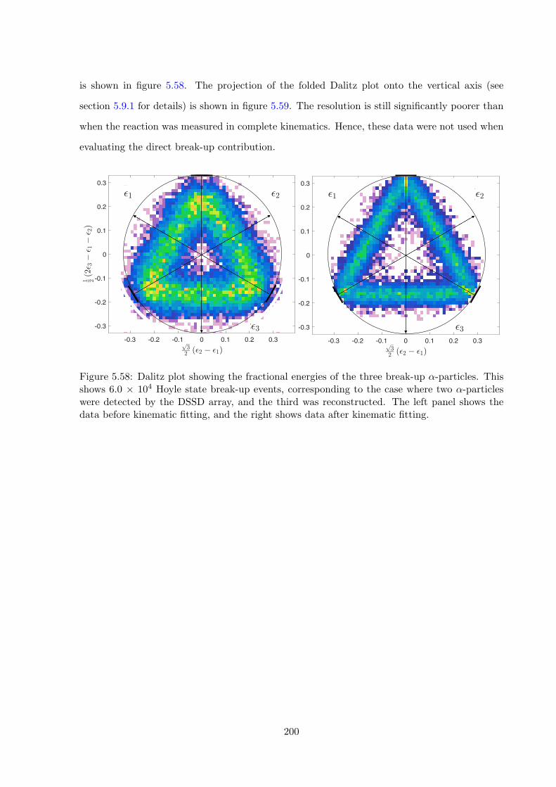
is shown in figure 5.58. The projection of the folded Dalitz plot onto the vertical axis (see

section 5.9.1 for details) is shown in figure 5.59. The resolution is still significantly poorer than

when the reaction was measured in complete kinematics. Hence, these data were not used when

evaluating the direct break-up contribution.

-0.3 -0.2 -0.1 0 0.1 0.2 0.3��

� ��� � ���

-0.3

-0.2

-0.1

0

0.1

0.2

0.3

� ���� ��� ��� �

�

0

5

10

15

20

25

30

35

40

45-0.3 -0.2 -0.1 0 0.1 0.2 0.3��

� ��� � ���

-0.3

-0.2

-0.1

0

0.1

0.2

0.3

� ���� ��� ��� �

�

0

2

4

6

8

10

12

14

-0.3 -0.2 -0.1 0 0.1 0.2 0.3��

� ��� � ���

-0.3

-0.2

-0.1

0

0.1

0.2

0.3

� ���� ��� ��� �

�

0

2

4

6

8

10

12

14

-0.3-0.2

-0.10

0.10.2

0.3�

����

���� �

-0.3

-0.2

-0.10

0.1

0.2

0.3

�� ���� � �� � ���

0 2 4 6 8 10 12 14

-0.3 -0.2 -0.1 0 0.1 0.2 0.3��

� ��� � ���

-0.3

-0.2

-0.1

0

0.1

0.2

0.3

� ���� ��� ��� �

�

0

10

20

30

40

50

60

70

80-0.3 -0.2 -0.1 0 0.1 0.2 0.3��

� ��� � ���

-0.3

-0.2

-0.1

0

0.1

0.2

0.3

� ���� ��� ��� �

�

0

2

4

6

8

10

12

14

-0.3 -0.2 -0.1 0 0.1 0.2 0.3��

� ��� � ���

-0.3

-0.2

-0.1

0

0.1

0.2

0.3� ���� ��� ��� �

�0

2

4

6

8

10

12

14

-0.3-0.2

-0.10

0.10.2

0.3�

����

���� �

-0.3

-0.2

-0.10

0.1

0.2

0.3

�� ���� � �� � ���

0 2 4 6 8 10 12 14

Figure 5.58: Dalitz plot showing the fractional energies of the three break-up ↵-particles. Thisshows 6.0 ⇥ 104 Hoyle state break-up events, corresponding to the case where two ↵-particleswere detected by the DSSD array, and the third was reconstructed. The left panel shows thedata before kinematic fitting, and the right shows data after kinematic fitting.

200

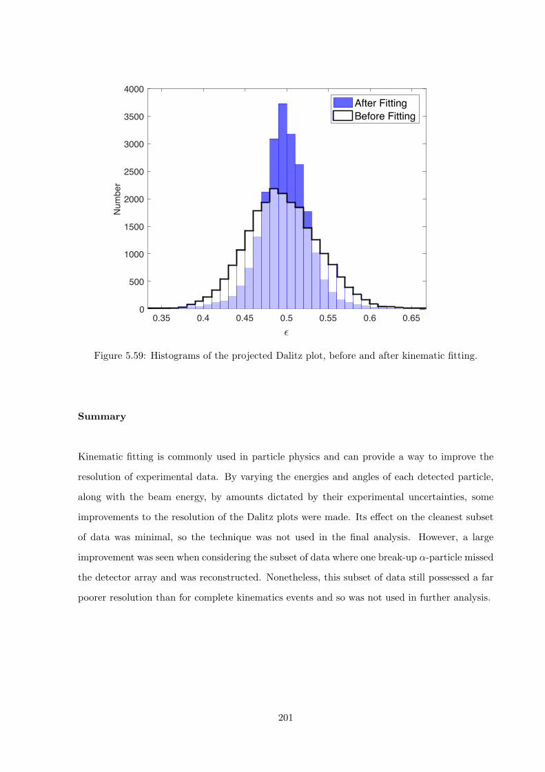
0.35 0.4 0.45 0.5 0.55 0.6 0.65�

0

500

1000

1500

2000

2500

3000

3500

4000

Num

ber

After FittingBefore Fitting

Figure 5.59: Histograms of the projected Dalitz plot, before and after kinematic fitting.

Summary

Kinematic fitting is commonly used in particle physics and can provide a way to improve the

resolution of experimental data. By varying the energies and angles of each detected particle,

along with the beam energy, by amounts dictated by their experimental uncertainties, some

improvements to the resolution of the Dalitz plots were made. Its e↵ect on the cleanest subset

of data was minimal, so the technique was not used in the final analysis. However, a large

improvement was seen when considering the subset of data where one break-up ↵-particle missed

the detector array and was reconstructed. Nonetheless, this subset of data still possessed a far

poorer resolution than for complete kinematics events and so was not used in further analysis.

201

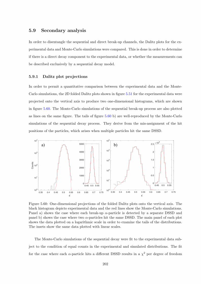
5.9 Secondary analysis

In order to disentangle the sequential and direct break-up channels, the Dalitz plots for the ex-

perimental data and Monte-Carlo simulations were compared. This is done in order to determine

if there is a direct decay component to the experimental data, or whether the measurements can

be described exclusively by a sequential decay model.

5.9.1 Dalitz plot projections

In order to permit a quantitative comparison between the experimental data and the Monte-

Carlo simulations, the 2D folded Dalitz plots shown in figure 5.51 for the experimental data were

projected onto the vertical axis to produce two one-dimensional histograms, which are shown

in figure 5.60. The Monte-Carlo simulations of the sequential break-up process are also plotted

as lines on the same figure. The tails of figure 5.60 b) are well-reproduced by the Monte-Carlo

simulations of the sequential decay process. They derive from the mis-assignment of the hit

positions of the particles, which arises when multiple particles hit the same DSSD.

0.35 0.4 0.45 0.5 0.55 0.6 0.65 0.7 0.75�

100

101

102

103

104

Cou

nts

0.35 0.4 0.45 0.5 0.55 0.6 0.65 0.7 0.75�

100

101

102

103

104

105

Cou

nts

0.45 0.5 0.55�

0

1000

2000

3000

4000

5000

Cou

nts

0.45 0.5 0.55�

0

0.5

1

1.5

2

2.5

Cou

nts

�104

a) b)

0.35 0.4 0.45 0.5 0.55 0.6 0.65 0.7 0.75�

100

101

102

103

104

Cou

nts

0.35 0.4 0.45 0.5 0.55 0.6 0.65 0.7 0.75�

100

101

102

103

104

Cou

nts

Figure 5.60: One-dimensional projections of the folded Dalitz plots onto the vertical axis. Theblack histogram depicts experimental data and the red lines show the Monte-Carlo simulations.Panel a) shows the case where each break-up ↵-particle is detected by a separate DSSD andpanel b) shows the case where two ↵-particles hit the same DSSD. The main panel of each plotshows the data plotted on a logarithmic scale in order to examine the tails of the distributions.The insets show the same data plotted with linear scales.

The Monte-Carlo simulations of the sequential decay were fit to the experimental data sub-

ject to the condition of equal counts in the experimental and simulated distributions. The fit

for the case where each ↵-particle hits a di↵erent DSSD results in a �2 per degree of freedom

202

of 1.16. The fit where two ↵-particles hit the same DSSD results in a �2 per degree of freedom

of 0.96. In both cases the fits lie close to the 50% confidence level in the �2 distributions. The

goodness of fit, without the inclusion of any direct decay component, indicates that the decay of

the Hoyle state is predominantly sequential. However, in order to determine if there are direct

decay contributions to the data, and decide which of the three-body break-up models are most

likely, these 1D histograms were compared with further Monte-Carlo simulations of the direct

decay processes discussed in section 5.8.7.

To illustrate the manifestation of each direct decay type on the one-dimensional projection

of the Dalitz plot, figures 5.61 and 5.62 were generated. The distribution of points for DD�,

DDE/DDP2 and DDL decay models, generated by the Monte-Carlo simulations, at the level of

0.1%, are shown overlaid on the experimental data. The e�ciencies for detecting each type of

decay are included in these plots, which is why some direct decay modes seem more prevalent

than others.

As described in section 5.1, reference [137] declared a 7.5% DDE decay contribution and a

9.5% DDL decay contribution. The 0.1% DD�, DDE/DDP2 and DDL distributions superim-

posed over the experimental data show that the claimed direct branching ratios are inconsistent

with the current data. The plots indicate that any direct decay contributions are much smaller

than these sources claim. Therefore, the present experimental data are more in line with refer-

ences [139] and [140], which measured no significant direct decay contributions.

203

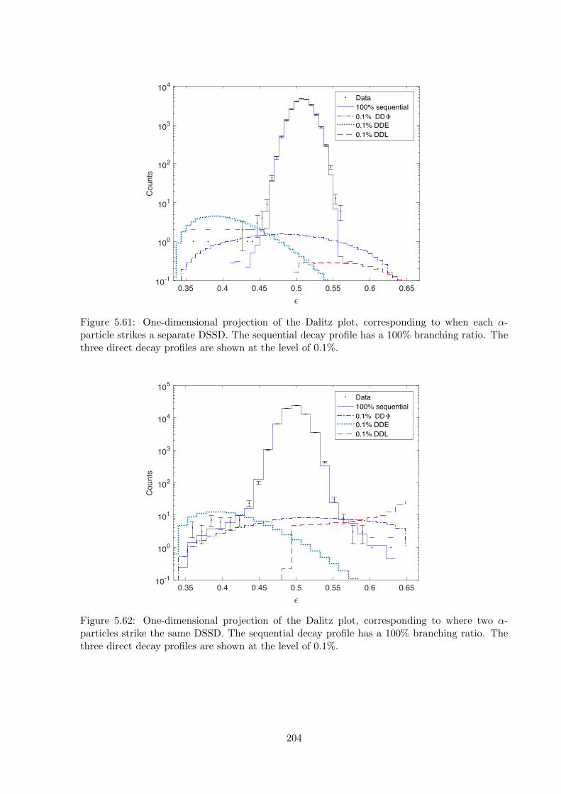
0.35 0.4 0.45 0.5 0.55 0.6 0.65�

10-1

100

101

102

103

104

Cou

nts

Data100% sequential0.1% DD�0.1% DDE0.1% DDL

Figure 5.61: One-dimensional projection of the Dalitz plot, corresponding to when each ↵-particle strikes a separate DSSD. The sequential decay profile has a 100% branching ratio. Thethree direct decay profiles are shown at the level of 0.1%.

0.35 0.4 0.45 0.5 0.55 0.6 0.65�

10-1

100

101

102

103

104

105

Cou

nts

Data100% sequential0.1% DD�0.1% DDE0.1% DDL

Figure 5.62: One-dimensional projection of the Dalitz plot, corresponding to where two ↵-particles strike the same DSSD. The sequential decay profile has a 100% branching ratio. Thethree direct decay profiles are shown at the level of 0.1%.

204

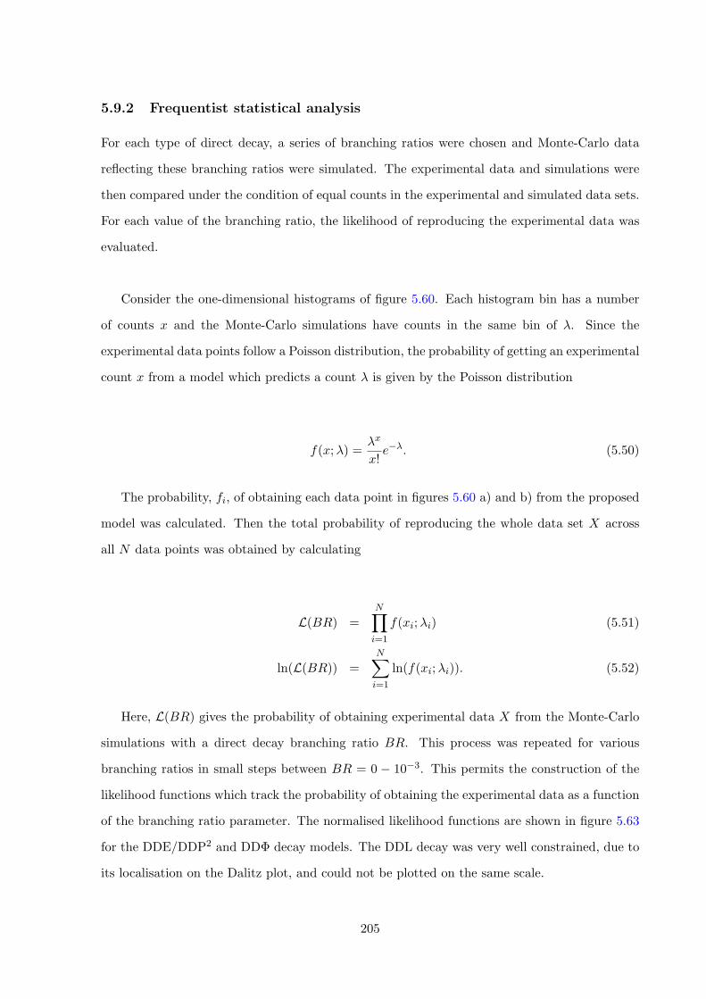
5.9.2 Frequentist statistical analysis

For each type of direct decay, a series of branching ratios were chosen and Monte-Carlo data

reflecting these branching ratios were simulated. The experimental data and simulations were

then compared under the condition of equal counts in the experimental and simulated data sets.

For each value of the branching ratio, the likelihood of reproducing the experimental data was

evaluated.

Consider the one-dimensional histograms of figure 5.60. Each histogram bin has a number

of counts x and the Monte-Carlo simulations have counts in the same bin of �. Since the

experimental data points follow a Poisson distribution, the probability of getting an experimental

count x from a model which predicts a count � is given by the Poisson distribution

f(x;�) =�x

x!e��. (5.50)

The probability, fi, of obtaining each data point in figures 5.60 a) and b) from the proposed

model was calculated. Then the total probability of reproducing the whole data set X across

all N data points was obtained by calculating

L(BR) =NY

i=1

f(xi;�i) (5.51)

ln(L(BR)) =NX

i=1

ln(f(xi;�i)). (5.52)

Here, L(BR) gives the probability of obtaining experimental data X from the Monte-Carlo

simulations with a direct decay branching ratio BR. This process was repeated for various

branching ratios in small steps between BR = 0 � 10�3. This permits the construction of the

likelihood functions which track the probability of obtaining the experimental data as a function

of the branching ratio parameter. The normalised likelihood functions are shown in figure 5.63

for the DDE/DDP2 and DD� decay models. The DDL decay was very well constrained, due to

its localisation on the Dalitz plot, and could not be plotted on the same scale.

205

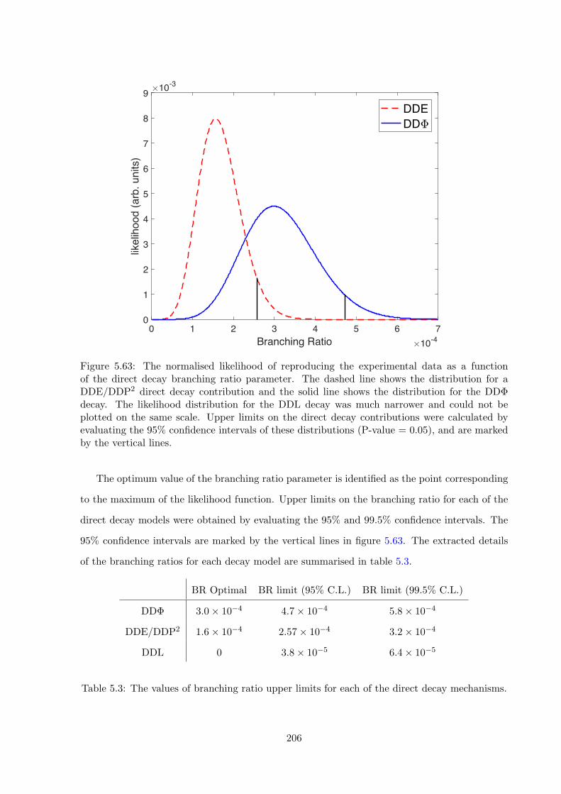
0 1 2 3 4 5 6 7Branching Ratio �10-4

0

1

2

3

4

5

6

7

8

9

likel

ihoo

d (a

rb. u

nits

)

�10-3

DDEDD�

Figure 5.63: The normalised likelihood of reproducing the experimental data as a functionof the direct decay branching ratio parameter. The dashed line shows the distribution for aDDE/DDP2 direct decay contribution and the solid line shows the distribution for the DD�decay. The likelihood distribution for the DDL decay was much narrower and could not beplotted on the same scale. Upper limits on the direct decay contributions were calculated byevaluating the 95% confidence intervals of these distributions (P-value = 0.05), and are markedby the vertical lines.

The optimum value of the branching ratio parameter is identified as the point corresponding

to the maximum of the likelihood function. Upper limits on the branching ratio for each of the

direct decay models were obtained by evaluating the 95% and 99.5% confidence intervals. The

95% confidence intervals are marked by the vertical lines in figure 5.63. The extracted details

of the branching ratios for each decay model are summarised in table 5.3.

BR Optimal BR limit (95% C.L.) BR limit (99.5% C.L.)

DD� 3.0⇥ 10�4 4.7⇥ 10�4 5.8⇥ 10�4

DDE/DDP2 1.6⇥ 10�4 2.57⇥ 10�4 3.2⇥ 10�4

DDL 0 3.8⇥ 10�5 6.4⇥ 10�5

Table 5.3: The values of branching ratio upper limits for each of the direct decay mechanisms.

206

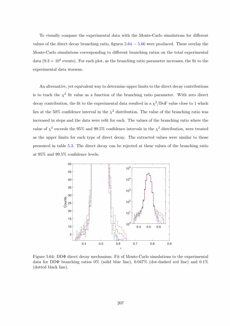
To visually compare the experimental data with the Monte-Carlo simulations for di↵erent

values of the direct decay branching ratio, figures 5.64 � 5.66 were produced. These overlay the

Monte-Carlo simulations corresponding to di↵erent branching ratios on the total experimental

data (9.3 ⇥ 104 events). For each plot, as the branching ratio parameter increases, the fit to the

experimental data worsens.

An alternative, yet equivalent way to determine upper limits to the direct decay contributions

is to track the �2 fit value as a function of the branching ratio parameter. With zero direct

decay contribution, the fit to the experimental data resulted in a �2/DoF value close to 1 which

lies at the 50% confidence interval in the �2 distribution. The value of the branching ratio was

increased in steps and the data were refit for each. The values of the branching ratio where the

value of �2 exceeds the 95% and 99.5% confidence intervals in the �2 distribution, were treated

as the upper limits for each type of direct decay. The extracted values were similar to those

presented in table 5.3. The direct decay can be rejected at these values of the branching ratio

at 95% and 99.5% confidence levels.

0.4 0.5 0.6 0.7 0.8 0.9�

5

10

15

20

25

30

35

40

45

50

Cou

nts

0.4 0.5 0.6�

100

101

102

103

104

105

Cou

nts

Figure 5.64: DD� direct decay mechanism: Fit of Monte-Carlo simulations to the experimentaldata for DD� branching ratios 0% (solid blue line), 0.047% (dot-dashed red line) and 0.1%(dotted black line).

207

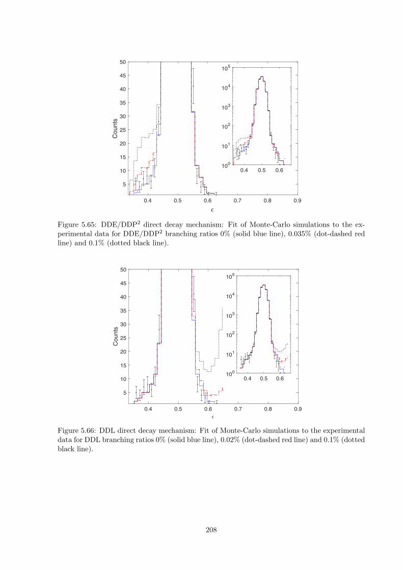
0.4 0.5 0.6 0.7 0.8 0.9�

5

10

15

20

25

30

35

40

45

50

Cou

nts

0.4 0.5 0.6�

100

101

102

103

104

105

Cou

nts

Figure 5.65: DDE/DDP2 direct decay mechanism: Fit of Monte-Carlo simulations to the ex-perimental data for DDE/DDP2 branching ratios 0% (solid blue line), 0.035% (dot-dashed redline) and 0.1% (dotted black line).

0.4 0.5 0.6 0.7 0.8 0.9�

5

10

15

20

25

30

35

40

45

50

Cou

nts

0.4 0.5 0.6�

100

101

102

103

104

105

Cou

nts

Figure 5.66: DDL direct decay mechanism: Fit of Monte-Carlo simulations to the experimentaldata for DDL branching ratios 0% (solid blue line), 0.02% (dot-dashed red line) and 0.1% (dottedblack line).

208

Summary

One-dimensional projections of the experimental Dalitz plots were fit with the equivalent plots

for the simulated data, with the condition of equal counts in the experimental and simulated

spectra. After accounting for the di↵erent detection e�ciencies, the likelihood of reproducing

the experimental spectrum was evaluated for various values of the direct decay branching ratio

used in the simulations. The likelihood plots as a function of the branching ratio were used to

evaluate the 95% and 99.5% confidence intervals, in order to place an upper limit on the direct

decay contribution. The results are summarised in table 5.3. An equivalent analysis, which

tracked the value of �2 as a function of the branching ratio, gave the same results.

209

5.9.3 Bayesian statistical analysis

In addition to the frequentist analysis, Bayesian inference was also used to determine an upper

limit on the DD� direct decay branching ratio of the Hoyle state.

Bayesian statistics is often contrasted with the classical frequentist statistics, which assumes

that measured phenomena are generated by a fixed, unknown process. In particular, this classical

formulation assumes that parameters are unknown constants, given that a complete knowledge

about a system is not available. The concept of probability is then used to describe the outcomes

of experimental measurements.

Bayesian statistics, on the other hand, assumes that parameters, although not known ex-

actly, are quantifiable random variables which can be described by probability distributions

[201]. Subjective probability distributions of parameters, called priors, are constructed based on

our experience and reasoning about these parameters. In this context, probability is interpreted

as a degree of belief about the values of the parameter under investigation. Once we collect new

experimental data, these are combined with the proposed prior distribution to create a new dis-

tribution called the posterior, which represents our current and updated probability assessment

of the parameters. Our new understanding about the parameters value is contained within the

posterior.

In the context of the Hoyle state decay, we should not treat the direct decay branching ratio

as a completely unknown parameter, since two recent measurements have set upper limits for

DD� decay of 0.5% [139] and 0.2% [140] with 95% confidence. Therefore, we know with 95%

confidence that the branching ratio is less that 0.2%. The idea is to combine these previous re-

sults with the present experimental measurements in order to better constrain the direct decay

branching ratio. Specifying the prior distribution is a controversial topic, due to the obvious

influence it has on the result. However, as shall be seen for the present data, the impact of the

prior is diminished as we gather more observations.

Previous experiments have also placed limits on the DDE and DDL decay branching ratios.

210

However, a standard definition of each of these decay modes was not observed. Therefore, prior

information about branching ratios for these processes was not incorporated in the present study.

For example, reference [139] assumed that a DDL decay comprised of a collinear decay where

two of the ↵-particles existed in the 8Be ground state resonance. In the present study, we instead

permit any collinear decay to belong to the DDL decay model. Similarly, reference [139] assumed

that for the DDE decay mechanism all three ↵-particles have exactly the same energies. The

present study and reference [140] assert that there must be must be an uncertainty/ smearing

of their energies due to their initial confinement inside the nucleus.

The formulation of Bayesian statistics is summarised by Bayes theorem, which states

P (A|X) =P (X|A)P (A)

P (X), (5.53)

where P (X|A) is the probability of measuring experimental data X given a physical model A.

The prior probability distribution (our current knowledge about the model A) is given by P (A).

The term, P (X), is a normalising constant to ensure that the total probability is 1. This allows

us to calculate the important quantity P (A|X), which is the probability of model A being true,

given the experimental data X. In a frequentist analysis, one basically assumes that P (X|A) =

P (A|X) without inferring anything from the prior.

In a simple example consider a medical test which searches for a condition A and gives a

positive result X or a negative result Y . The test has an accuracy of 0.9; the probability of a

positive result X if you have the condition A is 90% and the probability of a negative result Y

if you do not have the condition A is also 90%. Therefore, in the frequentist approach, if you

get a positive test result, there is a 90% chance you have the condition. However, the Bayesian

result is di↵erent. The quantity that we actually require is P (A|X), the probability of having

the condition A, given the test result X. If the condition has a prevalence so that on average

10% of the population have it, P (A) = 0.1. In order to use Bayes theorem to calculate P (A|X),

we also need to calculate P (X), which is the total probability of measuring X regardless of the

state of the patient.

211

P (X)total = P (X)⇥ P (A) + P (Y )⇥ (1� P (A)) (5.54)

P (X) = (0.9⇥ 0.1) + (0.1⇥ 0.9) = 0.18 (5.55)

Substituting the relevant values into equation 5.53 you calculate

P (A|X) =P (X|A)P (A)

P (X)(5.56)

P (A|X) =0.9⇥ 0.1

0.18= 0.5. (5.57)

Therefore, perhaps surprisingly, if you measure a positive test result, the probability of the

patient having the condition is actually only 50%. The frequentist misses some important infor-

mation, and the prior knowledge that only 10% of the population have the medical condition is

crucial to obtain a meaningful probability. In a similar way, in the present analysis, it is possible

to test for direct decay while bearing in mind that an upper limit on its existence has already

been calculated at the level of 0.2% (95% confidence interval).

To apply Bayes theorem to the present experimental data, the alternative to null hypothesis

testing presented in reference [202] was used. Here, the branching ratio for direct decay, BR, is

treated as a model parameter, and our knowledge about the value of this parameter is treated

as a probability distribution. The prior knowledge about the parameter comes from reference

[140], which concludes that for DD� decays, there is a 95% probability that BR 2 ⇥ 10�3.

A number of prior probability distributions reflecting this result are shown in figure 5.67 and

were used in the calculation. For each of these distributions, 95% of their areas lie below the

branching ratio 2 ⇥ 10�3.

212

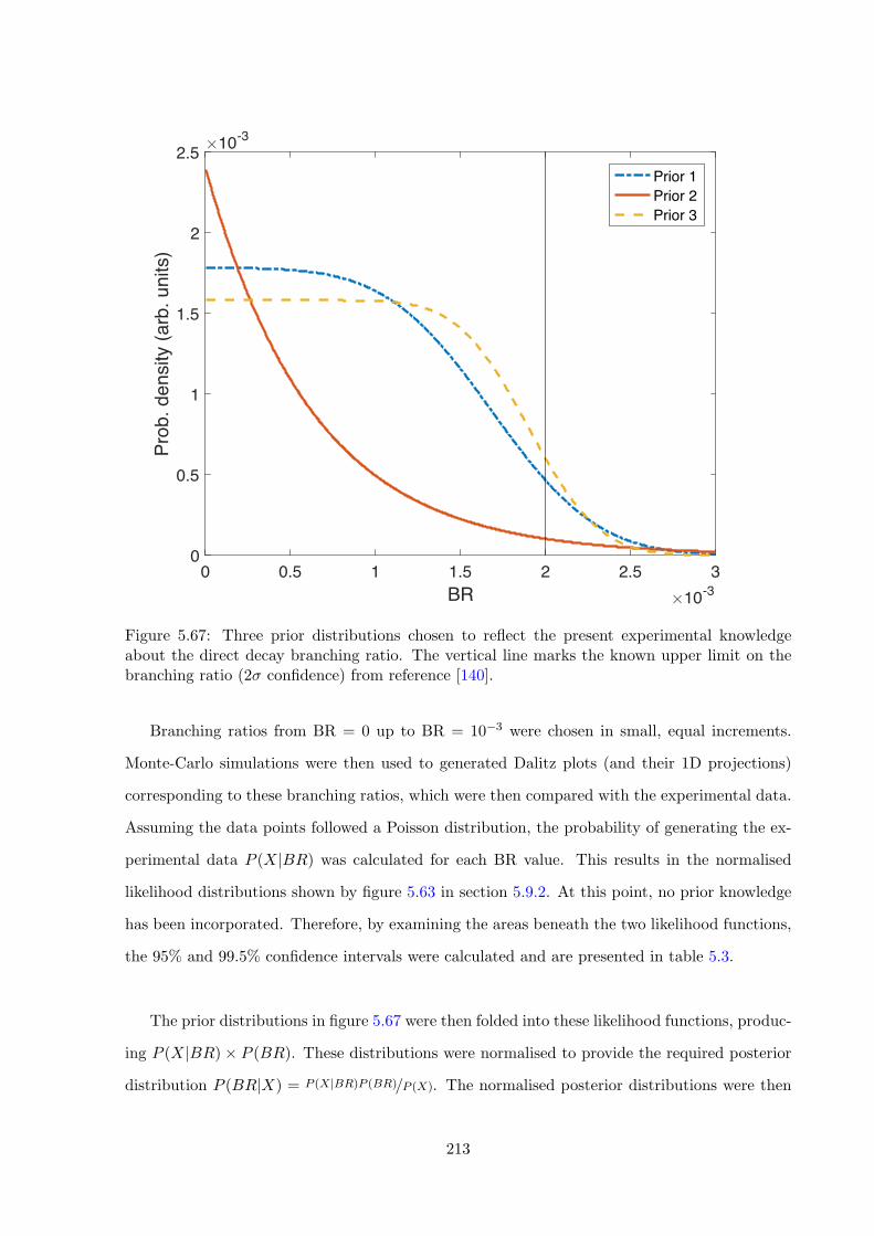
0 0.5 1 1.5 2 2.5 3BR �10-3

0

0.5

1

1.5

2

2.5Pr

ob. d

ensi

ty (a

rb. u

nits

)�10-3

Prior 1Prior 2Prior 3

Figure 5.67: Three prior distributions chosen to reflect the present experimental knowledgeabout the direct decay branching ratio. The vertical line marks the known upper limit on thebranching ratio (2� confidence) from reference [140].

Branching ratios from BR = 0 up to BR = 10�3 were chosen in small, equal increments.

Monte-Carlo simulations were then used to generated Dalitz plots (and their 1D projections)

corresponding to these branching ratios, which were then compared with the experimental data.

Assuming the data points followed a Poisson distribution, the probability of generating the ex-

perimental data P (X|BR) was calculated for each BR value. This results in the normalised

likelihood distributions shown by figure 5.63 in section 5.9.2. At this point, no prior knowledge

has been incorporated. Therefore, by examining the areas beneath the two likelihood functions,

the 95% and 99.5% confidence intervals were calculated and are presented in table 5.3.

The prior distributions in figure 5.67 were then folded into these likelihood functions, produc-

ing P (X|BR)⇥ P (BR). These distributions were normalised to provide the required posterior

distribution P (BR|X) = P (X|BR)P (BR)/P (X). The normalised posterior distributions were then

213

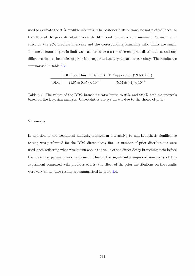
used to evaluate the 95% credible intervals. The posterior distributions are not plotted, because

the e↵ect of the prior distributions on the likelihood functions were minimal. As such, their

e↵ect on the 95% credible intervals, and the corresponding branching ratio limits are small.

The mean branching ratio limit was calculated across the di↵erent prior distributions, and any

di↵erence due to the choice of prior is incorporated as a systematic uncertainty. The results are

summarised in table 5.4.

BR upper lim. (95% C.I.) BR upper lim. (99.5% C.I.)

DD� (4.65± 0.05)⇥ 10�4 (5.67± 0.1)⇥ 10�4

Table 5.4: The values of the DD� branching ratio limits to 95% and 99.5% credible intervalsbased on the Bayesian analysis. Uncertainties are systematic due to the choice of prior.

Summary

In addition to the frequentist analysis, a Bayesian alternative to null-hypothesis significance

testing was performed for the DD� direct decay fits. A number of prior distributions were

used, each reflecting what was known about the value of the direct decay branching ratio before

the present experiment was performed. Due to the significantly improved sensitivity of this

experiment compared with previous e↵orts, the e↵ect of the prior distributions on the results

were very small. The results are summarised in table 5.4.

214

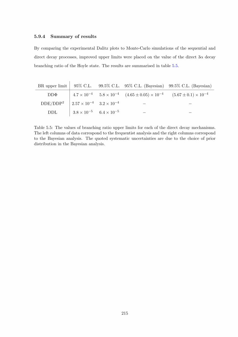
5.9.4 Summary of results

By comparing the experimental Dalitz plots to Monte-Carlo simulations of the sequential and

direct decay processes, improved upper limits were placed on the value of the direct 3↵ decay

branching ratio of the Hoyle state. The results are summarised in table 5.5.

BR upper limit 95% C.L. 99.5% C.L. 95% C.L. (Bayesian) 99.5% C.L. (Bayesian)

DD� 4.7⇥ 10�4 5.8⇥ 10�4 (4.65± 0.05)⇥ 10�4 (5.67± 0.1)⇥ 10�4

DDE/DDP2 2.57⇥ 10�4 3.2⇥ 10�4 � �DDL 3.8⇥ 10�5 6.4⇥ 10�5 � �

Table 5.5: The values of branching ratio upper limits for each of the direct decay mechanisms.The left columns of data correspond to the frequentist analysis and the right columns correspondto the Bayesian analysis. The quoted systematic uncertainties are due to the choice of priordistribution in the Bayesian analysis.

215

5.10 Interpretation of Results

The present experimental results build on numerous measurements of the direct decay of the

Hoyle state in the past [137–140]. The current experiment is unique in that it possessed the

sensitivity required to compare the experimental result with current theoretical predictions, cov-

ered in sections 5.4.3, 5.4.2 and 5.5. Notably, the result allows us to comment on the possible

↵-condensate nature of the Hoyle state.

In section 5.4.3, it was argued that for the decay of an ↵-condensed state into a number of

↵-condensed sub-systems, the branching ratio for each possibility should depend only on the

decay transmission probability and the available phase space. This was then estimated using

WKB Coulomb barrier penetrability calculations and found to be around 0.06%. The present

results reject the direct decay of the Hoyle state at the levels

DD� > 0.047%, DDE/DDP2 > 0.026% and DDL > 0.004%.

The upper limits for each proposed direct decay model are below the calculated phase space

limit. An enhancement of the 8Be + ↵ channel compared with this limit indicates that the

↵-condensate model may not be a good approximation of the Hoyle state. A dominant 8Be + ↵

structure, such as that predicted by AMD and FMD calculations [146, 153] seems more likely.

Furthermore, in 2014, Ishikawa performed a theoretical study into the decay of the Hoyle

state, using a full three-body quantum mechanical formulation [178]. In that work, the Hoyle

state is considered to be a system of three bosonic ↵-particles. The decay amplitude was evalu-

ated as a function of the momenta of the emitted ↵-particles and hence, the form of the Dalitz

plot was calculated. Ishikawa concluded that the number of events lying on a triangular locus in

the Dalitz plot, which are interpreted as sequential decay, would amount to 99.9% of the total.

No previous experiment has had the sensitivity to confirm or reject this proposed 0.1% direct

decay contribution. The present experimental measurements reject a direct decay contribution

> 0.047%, which is a factor of two lower than Ishikawa’s theoretical prediction. More specifi-

cally, the calculations predict

216

Total ⇡ 0.1%, DDE = 0.005% and DDL = 0.03%.

This disagreement with the experimental data indicates that the theoretical treatment of

the three ↵-particle constituents of the Hoyle state as bosons is an incorrect approach, casting

doubts on the BEC interpretation. The current experiment has rejected a DDL contribution

below this level, but did not have the sensitivity to test the proposed DDE contribution.

217

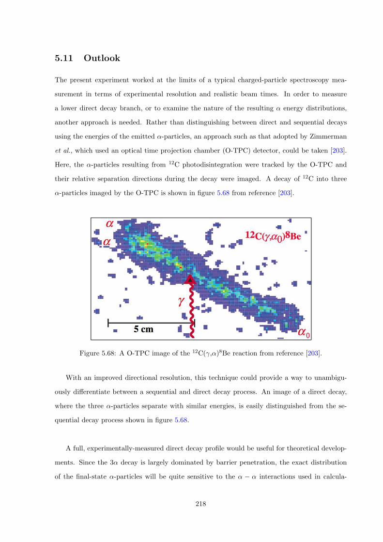
5.11 Outlook

The present experiment worked at the limits of a typical charged-particle spectroscopy mea-

surement in terms of experimental resolution and realistic beam times. In order to measure

a lower direct decay branch, or to examine the nature of the resulting ↵ energy distributions,

another approach is needed. Rather than distinguishing between direct and sequential decays

using the energies of the emitted ↵-particles, an approach such as that adopted by Zimmerman

et al., which used an optical time projection chamber (O-TPC) detector, could be taken [203].

Here, the ↵-particles resulting from 12C photodisintegration were tracked by the O-TPC and

their relative separation directions during the decay were imaged. A decay of 12C into three

↵-particles imaged by the O-TPC is shown in figure 5.68 from reference [203].

Figure 5.68: A O-TPC image of the 12C(�,↵)8Be reaction from reference [203].

With an improved directional resolution, this technique could provide a way to unambigu-

ously di↵erentiate between a sequential and direct decay process. An image of a direct decay,

where the three ↵-particles separate with similar energies, is easily distinguished from the se-

quential decay process shown in figure 5.68.

A full, experimentally-measured direct decay profile would be useful for theoretical develop-

ments. Since the 3↵ decay is largely dominated by barrier penetration, the exact distribution

of the final-state ↵-particles will be quite sensitive to the ↵ � ↵ interactions used in calcula-

218

tions. Therefore, reproducibility of the direct decay profile could form an excellent test for

realistic interaction potentials. In terms of theoretical input, more calculations of the direct

decay branching ratios, based on various models, would be welcome.

219

Chapter 6

Resistive strip detector

improvements

The two experiments presented in this thesis both detected charged particles using double-sided

silicon strip detectors. These consist of vertical front strips and horizontal rear strips. The

energy collected by a single front and single rear strip should be the same when a particle is

stopped in the detector. Therefore, by matching the energies collected by the front and rear

strips, the crossing point provides the position of the hit. The direction of the detected particle

can then be inferred. However, when there is a high multiplicity of particles, or the particles

have similar energies, it is possible to mis-assign their hit positions, as discussed in section 5.7.

In these instances, it may be advantageous to use a di↵erent type of detector called a resistive

charge division strip detector. These detectors have strips running only in one direction, but

have electrical contacts at each end of the strip. The strip itself carries a large resistance,

meaning that the signal, measured at each end of the strip, is proportional to the position of

the hit along the strip. Although these detectors have their advantages for certain applications,

they also have some major downfalls, such as being more susceptible to electronic noise. The

following paper, which will be submitted to Nuclear Instruments and Methods A in the near

future, aims to address some of these problems using novel techniques in the hardware and in

post-processing.

221

Chapter 7

Summary

At the end of this thesis, which details several di↵erent experiments, it is useful to reflect on how

these elements all fit together, and the overall contribution that this work has made towards the

field of nuclear physics.

Carbon-12

Foremost, the question of whether Bose-Einstein condensates can manifest in atomic nuclei

is something that has been speculated for a number of years, and has strongly influenced the

treatment of near-threshold states in ↵-conjugate nuclei. Due to its large radius, the Hoyle

state in 12C has long been seen as the ideal candidate nuclear state for this phenomenon to

occur. However, despite the fact that this theory very successfully predicts some properties of

this state, such as the charge form factor for inelastic electron excitation from the ground state

to the Hoyle state, this is not a unique description, and an unambiguous test of this structure

had not been performed.

The work presented in chapter 5 has unambiguously indicated that the interpretation of

Hoyle state as an ↵-condensate is problematic. In order to achieve this, a challenging, high

precision measurement of the direct 3↵ decay of this state was required. Under the assumption

of an ↵-condensed state, the direct 3↵ decay branching ratio should lie at 0.06%, given that the

branching ratio should depend only on the phase space and barrier penetrability for the decay.

The previous best measurement of this quantity was only able to place an upper limit on the

236

branching ratio at 0.2% [140]. The present work has set an upper limit at 0.047% or 0.026%,

depending on the type of direct decay that was considered.

Several improvements in the experimental method and analysis were required in order to

come to these conclusions. First of all, a novel detector geometry was implemented in order

to reduce the dominant experimental background. Implementing a quadrant array of DSSDs

to detect the three break-up ↵-particles permitted each to strike a separate DSSD, and remove

the ambiguity regarding their hit positions, which is a problem when multiple particles hit the

same detector. Utilising a large number of detectors and placing them further away from the

target also improved the angular granularity of the detectors. This is the dominant contribution

towards the resolution of the Dalitz plot, and hence, the sensitivity to direct decay. A large

number of decays were measured in order to collect the statistics required to reject the direct

decay at the quoted levels. To achieve this, a long experimental run of over 60 cumulative hours

was performed on the in-house Birmingham MC40 cyclotron.

Regarding the experimental analysis, the present study has been the first to link the abso-

lute value of the direct decay branching ratio with a signature for an ↵-condensate structure.

Reference [180] noted that for an ↵-condensate state, a break-up into any set of ↵-condensed

subsystems should be equally probable, as a reflection of the common wave functions of the

↵-particles in the initial state. In the case of the Hoyle state, the propensity for decays through

the 8Be ground state and the rare direct 3↵ decay channel, should dictated purely by the phase

space for the decay and the relative transmission probabilities through the Coulomb barrier. By

considering these factors, it was calculated in section 5.5 that the break-up branching ratio for

direct 3↵ decay should be ⇡0.06%. The present experiment has rejected the direct decay at

levels consistently below this value, indicating that there is a problem with the ↵-condensate

interpretation of the Hoyle state. A full quantum mechanical three-body calculation for the

decay of the Hoyle state has also been performed in the past, and found that a total direct de-

cay contribution of ⇡0.1% is expected [178]. This calculation treated the ↵-particles as bosons;

its disagreement with the current experimental data indicates that this may not be the correct

approach.

237

Previous experimental studies used a phenomenological DD� direct decay profile as the stan-

dard for searching for direct decays [138–140]. In this model, equal probabilities for direct decays

to anywhere in the available phase space are considered. However, this simple model does not

account for the significant changes in the transmission probability through the Coulomb barrier,

depending on the relative orientations of the three ↵-particles. For example, a decay where the

↵-particles emerge with the same energies has a much lower Coulomb barrier than the case where

one ↵-particle remains at rest. Therefore, there is a higher probability of the former situation

occurring. By utilising WKB calculations in hyperspherical coordinates, the present study has

developed a new direct decay profile, DDP2, which quantifies this e↵ect. Its manifestation was

found to be almost identical to that of the DDE profile used in the present study and in reference

[140]. It is this modified direct decay profile that should be considered in future studies, since

it more accurately describes the decaying system.

Beryllium-9

The Beryllium-9 nucleus has been long thought to possess a molecular structure. In this

picture, the two ↵-particles of the highly-clustered, unbound 8Be, are thought to become bound

by the exchange of a neutron. The valence neutron may occupy a number of di↵erent molecular

orbitals about the two ↵-particle cores; these are expected to have di↵erent angular momenta

and parities, and correspond to di↵erent amounts of deformation in the nucleon density. For

example, the ⇡-binding configuration has a more compact geometry than the �-binding con-

figuration. Since the 9Be system is deformed, the nucleus can rotate collectively, leading to

rotational bands, which are built on top of the di↵erent intrinsic molecular configurations. Until

this study, evidence has been found for three rotational bands in 9Be, corresponding to the

collective rotations of the ⇡-binding, �-binding and �-antibinding molecular states.

The present experiment has identified a previously unmeasured level in the 9Be spectrum at

3.8 MeV, which may correspond to the ⇡-antibinding molecular configuration. By comparing

with a newly-measured level in the mirror nucleus, 9B, and assuming that the reduced widths

for 8Beg.s. + n decay are the same for the two states, a firm limit on its angular momentum

was placed at J < 7/2. This leaves the possibility that the level does correspond to the hitherto

238

unmeasured ⇡-antibinding state. More work is needed to explore this possibility and future

experimental work has been proposed.

Since the unbound resonances of 9Be are very broad, they strongly overlap and make

analysing the states populated during an experiment di�cult. To overcome this, very high

statistics measurements were performed; data were collected for over 30 hours and a thick tar-

get was utilised. A novel method for reducing the energy losses in the thick target was developed.

Data were also acquired at two di↵erent beam energies, to ensure that any new features that

were identified were part of the 9Be spectrum, rather than manifestations of the many back-

ground reactions taking place.

Detector improvements

This investigation, which aimed to improve the performance of resistive charge division strip

detectors (RSDs), was in part motivated by the experimental challenges of measuring the di-

rect decay of the Hoyle state, detailed in this thesis. Since double-sided silicon strip detectors

(DSSDs) do not perform well for high multiplicity events where the detected particles have sim-

ilar energies, it was proposed that RSDs may provide a better alternative. However, although

the ambiguity in particle hit positions is not a problem when using RSDs, further issues are

encountered. Due to the charge division mechanism, the detectors are susceptible to noise,

meaning that they possess worse energy resolution and require higher discriminator thresholds

than DSSDs. Since there are fewer detector channels, RSDs also su↵er from more pile-up.

Two methods of reducing these backgrounds were developed. The first method utilised the

normally-unused rear contact of the RSD, which covers the whole of the detector area. By en-

suring that the sum of the energies detected by the front detector strips equalled that collected

by the rear detector contact, events where pile-up on a single strip or where a strip triggered

on noise could be omitted. This led to an improvement in the signal-to-background ratio by

around a factor of 4.

A second method was developed, which further improved the situation, by considering the

239

timing of the detections at each end of a detector strip. In a standard timing set-up, constant

fraction discriminators (CFDs) can be used to accurately measure the time of all of the detec-

tions in an event, with respect to a reference time. All detections associated with a single event

should fall within the same small time window. Placing a software gate on this time window

improves the signal-to-background ratio. However, in the absence of expensive CFDs, if leading

edge discriminators (LEDs) are used, timing information is smeared out due to time walk. The

present study showed that LEDs can be used for timing when using RSDs. If the time of the

pulses measured at each end of a detector strip are taken, due to the charge division, there

should be a fixed amount of time walk. By comparing the amount of time walk with the charge

division, detections falling within a correct time window could be identified and selected, leading

to an improvement in the signal-to-background ratio by a factor of around 3.5.

These methods can be utilised for any detector that uses resistive charge division in one

dimension. The TIARA array, presently located at one of the cyclotrons at Texas A&M, uses

Micron X1 resistive strip detectors, so the present methods could be applied there [204]. Due to

its ease of implementation in the hardware and in post-processing, the method of matching the

energies on front and rear detector contacts is most highly recommended at the present time.

240

Appendices

242

References

[1] R. Machleidt. “The nuclear force in the third millennium”. In: Nucl. Phys. A 689 (2001),

pp. 11 –22. issn: 0375-9474. doi: http://dx.doi.org/10.1016/S0375-9474(01)

00814-4. url: http://www.sciencedirect.com/science/article/pii/

S0375947401008144.

[2] H. D. Politzer. “Asymptotic freedom: An approach to strong interactions”. In: Phys.

Rep. 14 (1974), pp. 129 –180. issn: 0370-1573. doi: http://dx.doi.org/10.1016/

0370-1573(74)90014-3. url: http://www.sciencedirect.com/science/

article/pii/0370157374900143.

[3] A. Ekstrom, G. Baardsen, C. Forssen, G. Hagen, M. Hjorth-Jensen, G. R. Jansen, R.

Machleidt, W. Nazarewicz, T. Papenbrock, J. Sarich, and S. M. Wild. “Optimized Chiral

Nucleon-Nucleon Interaction at Next-to-Next-to-Leading Order”. In: Phys. Rev. Lett.

110 (2013), p. 192502. doi: 10.1103/PhysRevLett.110.192502. url: https:

//link.aps.org/doi/10.1103/PhysRevLett.110.192502.

[4] G. F. Knoll. Radiation detection and measurement. John Wiley & Sons, 2010.

[5] L. R. Hafstad and E. Teller. “The Alpha-Particle Model of the Nucleus”. In: Phys. Rev.

54 (1938), pp. 681–692. doi: 10.1103/PhysRev.54.681. url: https://link.

aps.org/doi/10.1103/PhysRev.54.681.

[6] M. Freer. “The clustered nucleus: cluster structures in stable and unstable nuclei”. In:

Rep. Prog. Phys. 70 (2007), p. 2149. url: http://stacks.iop.org/0034-4885/

70/i=12/a=R03.

[7] J.-P. Ebran, E. Khan, T. Niksic, and D. Vretenar. “How atomic nuclei cluster”. In: Nature

487 (2012), pp. 341–344.

287

[8] C. F. v. Weizsacker. “Zur Theorie der Kernmassen”. In: Z. Phys. A Hadron Nucl. 96

(1935), pp. 431–458. issn: 0044-3328. doi: 10.1007/BF01337700. url: http://dx.

doi.org/10.1007/BF01337700.

[9] J. Breithaupt. New understanding physics for advanced Level. IOP Publishing, 2000,

p. 162.

[10] N. Bohr and J. A. Wheeler. “The Mechanism of Nuclear Fission”. In: Phys. Rev. 56

(1939), pp. 426–450. doi: 10.1103/PhysRev.56.426. url: https://link.aps.

org/doi/10.1103/PhysRev.56.426.

[11] B. Cameron Reed. “Simple derivation of the Bohr–Wheeler spontaneous fission limit”.

In: Am. J. Phys. 71 (2003), pp. 258–260.

[12] J. Watterson. The Liquid Drop Model lecture slides. https://indico.cern.ch/

event/145296/contributions/1381141/attachments/136909/194250/

lecture17.pdf. Accessed: 24-05-2017.

[13] W. Demtroder. Atoms, molecules and photons. Springer, 2006.

[14] M. G. Mayer. “On Closed Shells in Nuclei”. In: Phys. Rev. 74 (1948), pp. 235–239. doi:

10.1103/PhysRev.74.235. url: https://link.aps.org/doi/10.1103/

PhysRev.74.235.

[15] R. D. Woods and D. S. Saxon. “Di↵use Surface Optical Model for Nucleon-Nuclei Scat-

tering”. In: Phys. Rev. 95 (1954), pp. 577–578. doi: 10.1103/PhysRev.95.577. url:

https://link.aps.org/doi/10.1103/PhysRev.95.577.

[16] O. Haxel, J. H. D. Jensen, and H. E. Suess. “On the ”Magic Numbers” in Nuclear

Structure”. In: Phys. Rev. 75 (1949), pp. 1766–1766. doi: 10.1103/PhysRev.75.

1766.2. url: https://link.aps.org/doi/10.1103/PhysRev.75.1766.2.

[17] R. Lawson. Theory of the nuclear shell model. Clarendon Press Oxford, 1980.

[18] A. Bohr and B. R. Mottelson. Nuclear structure. Vol. 1. World Scientific, 1998.

[19] Nuclear Deformation. http://www.wheldon.talktalk.net/thesis/thesis/

node10.html. Accessed: 20/08/2014.

[20] Nuclear Deformation Diagrams. http://creativecommons.org/licenses/by-

sa/3.0/http://en.wikipedia.org/wiki/Spheroid. Accessed: 22/09/2014.

288

[21] B. R. Mottelson and S. G. Nilsson. “Classification of the Nucleonic States in Deformed

Nuclei”. In: Phys. Rev. 99 (1955), pp. 1615–1617. doi: 10.1103/PhysRev.99.1615.

url: http://link.aps.org/doi/10.1103/PhysRev.99.1615.

[22] R Casten. Nuclear structure from a simple perspective. Vol. 6. Oxford University Press

Oxford, 2000.

[23] J. M. Brown and A. Carrington. Rotational spectroscopy of diatomic molecules. Cam-

bridge University Press, 2003.

[24] F. S. Stephens. “Coriolis e↵ects and rotation alignment in nuclei”. In: Rev. Mod. Phys.

47 (1975), pp. 43–65. doi: 10.1103/RevModPhys.47.43. url: https://link.

aps.org/doi/10.1103/RevModPhys.47.43.

[25] S. Kumar, J. Singh, J. K. Sharma, and S. Singh. “Coriolis E↵ects in Atomic Nuclei”. In:

International Journal of Computer Science and Communication Engineering IJCSCE

Special issue on “Emerging Trends in Engineering” ICETIE 2012 ().

[26] D. J. Rowe. Nuclear collective motion: models and theory. World Scientific, 2010, pp. 86–

87.

[27] Coriolis Force: an artefact of the earth’s rotation. http://ww2010.atmos.uiuc.

edu/(Gh)/guides/mtr/fw/crls.rxml. Accessed: 27/05/2017.

[28] W. von Oertzen, M. Freer, and Y. Kanada-En’yo. “Nuclear clusters and nuclear molecules”.

In: Phys. Rep. 432 (2006), pp. 43 –113. issn: 0370-1573. doi: https://doi.org/10.

1016/j.physrep.2006.07.001. url: http://www.sciencedirect.com/

science/article/pii/S0370157306002626.

[29] J. A. Peacock, S. Cole, P. Norberg, C. M. Baugh, J. Bland-Hawthorn, T. Bridges, R. D.

Cannon, M. Colless, C. Collins, W. Couch, et al. “A measurement of the cosmological

mass density from clustering in the 2dF Galaxy Redshift Survey”. In: Nature 410 (2001),

pp. 169–173.

[30] OS MACKEREL CONTRA O MUNDO. https://www.ideafixa.com/oldbutgold/

os-mackerel-contra-o-mundo. Accessed: 30/05/2017.

289

[31] K. Ikeda, N. Takigawa, and H. Horiuchi. “The systematic structure-change into the

molecule-like structures in the self-conjugate 4n nuclei”. In: Prog. Theor. Phys. Suppl. 68

(1968), pp. 464–475.

[32] K. Giovanetti.Matter Sources. http://csma31.csm.jmu.edu/physics/courses/

163/older/bigbang2.htm. Accessed: 30/05/2017.

[33] M. Freer, R. R. Betts, and A. H. Wuosmaa. “Relationship between the deformed har-

monic oscillator and clustering in light nuclei”. In: Nucl. Phys. A 587 (1995), pp. 36

–54. issn: 0375-9474. doi: http://dx.doi.org/10.1016/0375- 9474(94)

00820-D. url: http://www.sciencedirect.com/science/article/pii/

037594749400820D.

[34] O. R. Frisch, G. Hevesy, and H. A. C. McKay. “Selective Absorption of Neutrons by

Gold”. In: Nature 137 (1936), pp. 149–150.

[35] E. Amaldi and E. Fermi. “On the Absorption and the Di↵usion of Slow Neutrons”. In:

Phys. Rev. 50 (1936), pp. 899–928. doi: 10.1103/PhysRev.50.899. url: https:

//link.aps.org/doi/10.1103/PhysRev.50.899.

[36] G. Breit and E. Wigner. “Capture of Slow Neutrons”. In: Phys. Rev. 49 (1936), pp. 519–

531. doi: 10.1103/PhysRev.49.519. url: https://link.aps.org/doi/10.

1103/PhysRev.49.519.

[37] K. S. Krane and D. Halliday. Introductory nuclear physics. Vol. 465. Wiley New York,

1988.

[38] What is Nuclear Resonance � Compound Nucleus. http://www.nuclear-power.

net/nuclear-power/reactor-physics/nuclear-engineering-fundamentals/

neutron-nuclear-reactions/compound-nucleus-reactions/what-is-

nuclear-resonance-compound-nucleus/prettyPhoto. Accessed: 15-05-2017.

[39] J. Refsgaard. “Resonances, R-Matrix � Rotations in 12C?” PhD thesis. Institut for Fysik

go Astromomi Aarhus Universitet, 2016.

[40] A. M. Lane and R. G. Thomas. “R-Matrix Theory of Nuclear Reactions”. In: Rev. Mod.

Phys. 30 (1958), pp. 257–353. doi: 10.1103/RevModPhys.30.257. url: https:

//link.aps.org/doi/10.1103/RevModPhys.30.257.

290

[41] P. Descouvemont and D. Baye. “The R-matrix theory”. In: Rep. Prog. Phys. 73 (2010),

p. 036301. url: http://stacks.iop.org/0034-4885/73/i=3/a=036301.

[42] T. Teichmann and E. P. Wigner. “Sum Rules in the Dispersion Theory of Nuclear Reac-

tions”. In: Phys. Rev. 87 (1952), pp. 123–135. doi: 10.1103/PhysRev.87.123. url:

http://link.aps.org/doi/10.1103/PhysRev.87.123.

[43] C. Simenel, B. Avez, and D. Lacroix. “Microscopic approaches for nuclear Many-Body

dynamics: applications to nuclear reactions”. In: arXiv preprint arXiv:0806.2714 (2008).

[44] I. J. Thompson and F. M. Nunes. Nuclear reactions for astrophysics: principles, calcula-

tion and applications of low-energy reactions. Cambridge University Press, 2009, p. 347.

[45] F. C. Barker and P. B. Treacy. “Nuclear levels near thresholds”. In: Nucl. Phys. 38 (1962),

pp. 33 –49. issn: 0029-5582. doi: http://dx.doi.org/10.1016/0029-5582(62)

91014-3. url: http://www.sciencedirect.com/science/article/pii/

0029558262910143.

[46] F. C. Barker, H. J. Hay, and P. B Treacy. “0+ States of 8Be”. In: Austr. J. Phys. 21

(1968), pp. 239 –258.

[47] C. A. Diget, F. C. Barker, M. J. G. Borge, R. Boutami, P. Dendooven, T. Eronen, S.

P. Fox, B. R. Fulton, H. O. U. Fynbo, J. Huikari, S. Hyldegaard, H. B. Jeppesen, A.

Jokinen, B. Jonson, A. Kankainen, I. Moore, A. Nieminen, G. Nyman, H. Penttila, V.

F. E. Pucknell, K. Riisager, S. Rinta-Antila, O. Tengblad, Y. Wang, K. Wilhelmsen, and

J. Aysto. “Breakup channels for 12C triple-↵ continuum states”. In: Phys. Rev. C 80

(2009), p. 034316. doi: 10.1103/PhysRevC.80.034316. url: https://link.

aps.org/doi/10.1103/PhysRevC.80.034316.

[48] F. D. Becchetti, C. A. Fields, R. S. Raymond, H. C. Bhang, and D. Overway. “Ghost

anomaly in 8Be studied with 9Be(p,d) at Ep = 14.3 and 26.2 MeV”. In: Phys. Rev. C

24 (1981), pp. 2401–2408. doi: 10.1103/PhysRevC.24.2401. url: http://link.

aps.org/doi/10.1103/PhysRevC.24.2401.

[49] A. Szczurek, K. Bodek, L. Jarczyk, and J. K. et. al. “Ghost anomaly and first excited

state of 8Be in the 9Be(d,t)4He reaction at 7 MeV”. In: Nucl. Phys. A 531 (1991), pp. 77

–92. issn: 0375-9474. doi: http://dx.doi.org/10.1016/0375- 9474(91)

291

90569-R. url: http://www.sciencedirect.com/science/article/pii/

037594749190569R.

[50] E. H. Berkowitz, G. L. Marolt, A. A. Rollefson, and C. P. Browne. “Survey of the 8Be

Ghost Anomaly”. In: Phys. Rev. C 4 (1971), pp. 1564–1570. doi: 10.1103/PhysRevC.

4.1564. url: https://link.aps.org/doi/10.1103/PhysRevC.4.1564.

[51] AZURE2 R-Matrix Program. https://azure.nd.edu/login.php. Accessed: 22-

05-2017.

[52] D. Tilley, J. Kelley, J. Godwin, D. Millener, J. Purcell, C. Sheu, and H. Weller. “Energy

levels of light nuclei A=8,9,10”. In: Nucl. Phys. A 745 (2004), pp. 155 –362. issn: 0375-

9474. doi: http://dx.doi.org/10.1016/j.nuclphysa.2004.09.059. url:

http://www.sciencedirect.com/science/article/pii/S0375947404010267.

[53] M. Freer. “Molecules in nuclei”. In: C. R. Phys. 4 (2003), pp. 475–487.

[54] D. Scharnweber, W. Greiner, and U. Mosel. “The two-center shell model”. In: Nucl. Phys.

A 164 (1971), pp. 257–278.

[55] W. von Oertzen. “Two-center molecular states in 9B, 9Be, 10Be, and 10B”. In: Z. Phys. A

Hadron Nucl. 354 (1996), pp. 37–43. issn: 0939-7922. doi: 10.1007/s002180050010.

url: http://dx.doi.org/10.1007/s002180050010.

[56] F. Barker and C. Woods. “States of 5He and 5Li”. In: Austr. J. Phys. 38 (1985), pp. 563–

576.

[57] S. Okabe, Y. Abe, and H. Tanaka. “The Structure of 9Be Nucleus by a Molecular Model.

I)”. In: Prog. Theor. Phys. 57 (1977), p. 866. doi: 10.1143/PTP.57.866. eprint:

/oup/backfile/content_public/journal/ptp/57/3/10.1143/ptp.57.

866/2/57-3-866.pdf. url: http://dx.doi.org/10.1143/PTP.57.866.

[58] S. Okabe, Y. Abe, and H. Tanaka. “The Structure of 9Be by a Molecular Model. II”.

In: Prog. Theor. Phys. 61 (1979), p. 1049. doi: 10.1143/PTP.61.1049. eprint:

/oup/backfile/content_public/journal/ptp/61/4/10.1143/ptp.61.

1049/2/61-4-1049.pdf. url: +http://dx.doi.org/10.1143/PTP.61.1049.

292

[59] C. Adler, T. Corcoran, and C. Mast. “The application of the Su(3) shell model to 9Be”.

In: Nucl. Phys. 88 (1966), pp. 145 –168. issn: 0029-5582. doi: http://dx.doi.org/

10.1016/0029-5582(66)90457-3. url: http://www.sciencedirect.com/

science/article/pii/0029558266904573.

[60] A. G. Slight, T. E. Drake, and G. R. Bishop. “Inelastic electron scattering and the

electromagnetic properties of 9Be”. In: Nucl. Phys. A 208 (1973), pp. 157 –195. issn: 0375-

9474. doi: http://dx.doi.org/10.1016/0375-9474(73)90740-9. url: http:

//www.sciencedirect.com/science/article/pii/0375947473907409.

[61] M. A. Caprio, P. Maris, and J. Vary. “Emergence of rotational bands in ab initio no-

core configuration interaction calculations of light nuclei”. In: Phys. Lett. B 719 (2013),

pp. 179 –184. issn: 0370-2693. doi: https://doi.org/10.1016/j.physletb.

2012.12.064. url: http://www.sciencedirect.com/science/article/

pii/S0370269313000026.

[62] M. A. Caprio, P. Maris, J. P. Vary, and R. Smith. “Collective rotation from ab initio

theory”. In: Int. J. Mod. Phys. E 24 (2015), p. 1541002.

[63] P. Maris and J. P. Vary. “Ab initio nuclear structure calculations of p-shell nuclei with

JISP16”. In: Int. J. Mod. Phys. E 22 (2013), p. 1330016.

[64] R. C. Cockrell. “Ab initio nuclear structure calculations for light nuclei”. PhD thesis.

Iowa State University, 2012.

[65] H. Akimune, M. Fujimura, M. Fujiwara, K. Hara, T. Ishikawa, T. Kawabata, H. Ut-

sunomiya, T. Yamagata, K. Yamasaki, and M. Yosoi. “Evidence for a 3.8 MeV state in

9B”. In: Phys. Rev. C 64 (2001), p. 041305. doi: 10.1103/PhysRevC.64.041305.

url: https://link.aps.org/doi/10.1103/PhysRevC.64.041305.

[66] C. Scholl, Y. Fujita, T. Adachi, P. von Brentano, H. Fujita, M. Gorska, H. Hashimoto, K.

Hatanaka, H. Matsubara, K. Nakanishi, T. Ohta, Y. Sakemi, Y. Shimbara, Y. Shimizu,

Y. Tameshige, A. Tamii, M. Yosoi, and R. G. T. Zegers. “High-resolution study of

the 9Be(3He,t)9B reaction up to the 9B triton threshold”. In: Phys. Rev. C 84 (2011),

p. 014308. doi: 10.1103/PhysRevC.84.014308. url: https://link.aps.org/

doi/10.1103/PhysRevC.84.014308.

293

[67] C. Forssen, P. Navratil, W. E. Ormand, and E. Caurier. “Large basis ab initio shell

model investigation of 9Be and 11Be”. In: Phys. Rev. C 71 (4 2005), p. 044312. doi:

10.1103/PhysRevC.71.044312. url: https://link.aps.org/doi/10.1103/

PhysRevC.71.044312.

[68] R. Machleidt. “High-precision, charge-dependent Bonn nucleon-nucleon potential”. In:

Phys. Rev. C 63 (2 2001), p. 024001. doi: 10.1103/PhysRevC.63.024001. url:

https://link.aps.org/doi/10.1103/PhysRevC.63.024001.

[69] S. M. Lenzi. “Coulomb energy di↵erences in mirror nuclei”. In: J. Phys. Conf. Ser. Vol. 49.

IOP Publishing. 2006, p. 85.

[70] B. Agrawal, T. Sil, S. Samaddar, J. De, and S. Shlomo. “Coulomb energy di↵erences in

mirror nuclei revisited”. In: Phys. Rev. C 64 (2001), p. 024305.

[71] F. Zijderhand, R. Makkus, and C. V. D. Leun. “Investigation of 41Sc by proton capture

in 40Ca”. In: Nucl. Phys. A 466 (1987), pp. 280 –294. issn: 0375-9474. doi: http:

//dx.doi.org/10.1016/0375- 9474(87)90442- 8. url: http://www.

sciencedirect.com/science/article/pii/0375947487904428.

[72] C. Wheldon, T. Kokalova, M. Freer, J. Walshe, R. Hertenberger, H.-F. Wirth, N. I.

Ashwood, M. Barr, N. Curtis, T. Faestermann, R. Lutter, J. D. Malcolm, and D. J.

Marın-Lambarri. “Spectroscopy of 9B via high-resolution ejectile-tagged recoil break-

up”. In: Phys. Rev. C 91 (2015), p. 024308. doi: 10.1103/PhysRevC.91.024308.

url: https://link.aps.org/doi/10.1103/PhysRevC.91.024308.

[73] M. A. Bentley and S. M. Lenzi. “Coulomb energy di↵erences between high-spin states in

isobaric multiplets”. In: Prog. Part. Nucl. Phys. 59.2 (2007), pp. 497 –561. issn: 0146-

6410. doi: https://doi.org/10.1016/j.ppnp.2006.10.001. url: http:

//www.sciencedirect.com/science/article/pii/S0146641006000743.

[74] R. Smith, C. Wheldon, M. Freer, N. Curtis, T. Kokalova, S. Almaraz-Calderon, A. Apra-

hamian, N. I. Ashwood, M. Barr, B. Bucher, P. Copp, M. Couder, X. Fang, G. Goldring,

F. Jung, S. R. Lesher, W. Lu, J. D. Malcolm, A. Roberts, W. P. Tan, and V. A. Ziman.

“Evidence for a 3.8 MeV state in 9Be”. In: Phys. Rev. C 94 (2016), p. 014320. doi:

10.1103/PhysRevC.94.014320. url: https://link.aps.org/doi/10.1103/

PhysRevC.94.014320.

294

[75] F. C. Barker and N. Ferdous. “The Low-lying Levels of 13C and 13N”. In: Australian

Journal of Physics 33.4 (1980), pp. 691–718.

[76] R. G. Thomas. “An Analysis of the Energy Levels of the Mirror Nuclei, C13 and N13”.

In: Phys. Rev. 88 (5 1952), pp. 1109–1125. doi: 10.1103/PhysRev.88.1109. url:

https://link.aps.org/doi/10.1103/PhysRev.88.1109.

[77] J. B. Ehrman. “On the Displacement of Corresponding Energy Levels of C13 and N13”.

In: Phys. Rev. 81 (3 1951), pp. 412–416. doi: 10.1103/PhysRev.81.412. url:

https://link.aps.org/doi/10.1103/PhysRev.81.412.

[78] H. T. Fortune and R. Sherr. “Proton and alpha spectroscopic factors for states at 6.4˘7.5

MeV in 19Ne”. In: Phys. Rev. C 73 (2006), p. 024302. doi: 10.1103/PhysRevC.73.

024302. url: https://link.aps.org/doi/10.1103/PhysRevC.73.024302.

[79] Institute for Nuclear Structure and Astrophysics (ISNAP) Accelerators. http://isnap.

nd.edu/research/facility/accelerator/. Accessed: 21-04-2017.

[80] Van de Graa↵ generator dictionary definition. http://www.yourdictionary.com/

van-de-graaff-generator. Accessed: 20-07-2017.

[81] L. Lamm. FN Tandem Van de Graa↵ Accelerator at Notre Dame. http : / / www .

jinaweb.org/outreach/PIXE-PAN09/docs/Accelerator%20Presentation_

June2009.pdf. Accessed: 21-04-2017.

[82] N Curtis. Accelerators and Detectors. Lecture. 2014.

[83] H. Liebl. Applied charged particle optics. Vol. 2012. Springer, 2008, p. 39.

[84] DC Coupled Double Sided. http://www.micronsemiconductor.co.uk/products-

strip.asp?productsubcatID=2. Accessed: 20-12-2012.

[85] W. R. Leo. “Techniques for Nuclear and Particle Physics Experiments; A How-to Ap-

proach”. In: 48 (1993), p. 271.

[86] G. Knoll and D. Mcgregor. “Fundamentals of Semiconductor Detectors for Ionizing Ra-

diation”. In: MRS Proceedings 302 (1993). doi: 10.1557/PROC-302-3.

[87] K. Shah, J. Lund, and F. Olschner. “Charge collection e�ciency in a semiconductor

radiation detector with a non-constant electric field”. In: IEEE Trans. Nucl. Sci. 37

(1990), pp. 183–186.

295

[88] G. Lindstrom. “Radiation damage in silicon detectors”. In: Nucl. Instrum. Methods Phys.

Res. A 512 (2003), pp. 30–43.

[89] G. Casse. “The e↵ect of hadron irradiation on the electrical properties of particle detectors

made from various silicon materials”. PhD thesis. Universite Joseph Fourier - Grenoble,

Sept. 1998.

[90] R. Smith. Investigating Clustered States in 9Be through Inelastic Alpha Particle Scat-

tering. http://undergraduatelibrary.org/2013/mathematics-physics/

investigating-clustered-states-9be-nucleus-through-inelastic-

alpha-particle. Accessed: 24/09/2014.

[91] P. Busa. “Understanding Design and Operation of Successive Approximation Register”.

In: (2008). url: http://cmosedu.com/jbaker/courses/ece614/s08/lec23_

ece614.pdf.

[92] Multi Instance Data Acquisition System. http://npg.dl.ac.uk/MIDAS/. Accessed:

22-05-2017.

[93] S. M. Singer. Sunsort reference manual. http://npg.dl.ac.uk/MIDAS/manual/

SunSort/index.html. Accessed: 2017.

[94] R. Smith, M. Freer, C. Wheldon, N. Curtis, S. Almaraz-Calderon, A. Aprahamian, N. I.

Ashwood, M. Barr, B. Bucher, P. Copp, et al. “Breakup branches of Borromean beryllium-

9”. In: AIP Conference Proceedings. Vol. 1681. AIP Publishing. 2015, p. 060003.

[95] T. W. Armstrong and K. C. Chandler. A Fortran program for computing stopping powers

and ranges for muons, charged pions, protons, and heavy ions. ORNL-4869, Oak Ridge

National Laboratory. Accessed: 27-04-2017. 1973.

[96] T. Armstrong and K. Chandler. “SPAR, a FORTRAN program for computing stopping

powers and ranges for muons, charged pions, protons, and heavy ions”. In: ORNL-4869,

Oak Ridge National Laboratory (1973).

[97] H. Bethe and J. Ashkin. Nuclear structure from a simple perspective. J Wiley, New York,

1953, p. 253.

[98] J. Lindhard, M. Schar↵, and H. E. Schiøtt. Range concepts and heavy ion ranges. Munks-

gaard Copenhagen, 1963.

296

[99] P. Papka, T. A. D. Brown, B. R. Fulton, D. L. Watson, S. P. Fox, D. Groombridge, M.

Freer, N. M. Clarke, N. I. Ashwood, N. Curtis, V. Ziman, P. McEwan, S. Ahmed, W.

N. Catford, D. Mahboub, C. N. Timis, T. D. Baldwin, and D. C. Weisser. “Decay path

measurements for the 2.429 MeV state in 9Be: Implications for the astrophysical ↵+↵+n

reaction”. In: Phys. Rev. C 75 (2007), p. 045803. doi: 10.1103/PhysRevC.75.

045803. url: https://link.aps.org/doi/10.1103/PhysRevC.75.045803.

[100] T. A. D. Brown, P. Papka, B. R. Fulton, D. L. Watson, S. P. Fox, D. Groombridge, M.

Freer, N. M. Clarke, N. I. Ashwood, N. Curtis, V. Ziman, P. McEwan, S. Ahmed, W. N.

Catford, D. Mahboub, C. N. Timis, T. D. Baldwin, and D. C. Weisser. “Decay studies

for states in 9Be up to 11 MeV: Insights into the n+8Be and ↵+5He cluster structure”.

In: Phys. Rev. C 76 (2007), p. 054605. doi: 10.1103/PhysRevC.76.054605. url:

https://link.aps.org/doi/10.1103/PhysRevC.76.054605.

[101] N. Curtis, N. M. Clarke, B. R. Fulton, S. J. Hall, M. J. Leddy, A. S. J. Murphy, J. S.

Pople, R. P. Ward, W. N. Catford, G. J. Gyapong, S. M. Singer, S. P. G. Chappell,

S. P. Fox, C. D. Jones, D. L. Watson, W. D. M. Rae, and P. M. Simmons. “”Association

of the 12C+12C breakup states in 24Mg with the quasimolecular resonances””. In: Phys.

Rev. C 51 (1995), pp. 1554–1557. doi: 10.1103/PhysRevC.51.1554. url: http:

//link.aps.org/doi/10.1103/PhysRevC.51.1554.

[102] N. Curtis, A. S. J. Murphy, N. M. Clarke, M. Freer, B. R. Fulton, S. J. Hall, M. J. Leddy,

J. S. Pople, G. Tungate, R. P. Ward, W. N. Catford, G. J. Gyapong, S. M. Singer, S.

P. G. Chappell, S. P. Fox, C. D. Jones, D. L. Watson, W. D. M. Rae, P. M. Simmons,

and P. H. Regan. “Evidence for a highly deformed band in 16O+16O breakup of 32S”.

In: Phys. Rev. C 53 (1996), pp. 1804–1810. doi: 10.1103/PhysRevC.53.1804. url:

http://link.aps.org/doi/10.1103/PhysRevC.53.1804.

[103] N. Curtis. PhD thesis. University of Birmingham, 1995.

[104] M. A. Tiede, K. W. Kemper, N. R. Fletcher, D. Robson, D. D. Caussyn, S. J. Bennett, J.

D. Brown, W. N. Catford, C. D. Jones, D. L. Watson, and W. D. M. Rae. “Measurement

of low-lying states in 9B”. In: Phys. Rev. C 52 (1995), pp. 1315–1325. doi: 10.1103/

PhysRevC.52.1315. url: https://link.aps.org/doi/10.1103/PhysRevC.

52.1315.

297

[105] R. E. Azuma, E. Uberseder, E. C. Simpson, C. R. Brune, H. Costantini, R. J. de

Boer, J. Gorres, M. Heil, P. J. LeBlanc, C. Ugalde, and M. Wiescher. “AZURE: An

R-matrix code for nuclear astrophysics”. In: Phys. Rev. C 81 (2010), p. 045805. doi:

10.1103/PhysRevC.81.045805. url: https://link.aps.org/doi/10.1103/

PhysRevC.81.045805.

[106] R. Smith. Tracey Peaker version 1.0 peak fitting code. Matlab File Exchange, 57125.

Accessed: 12-05-2016.

[107] F. Ajzenberg-Selove. “Energy levels of light nuclei A = 1112”. In: Nucl. Phys. A 506

(1990), pp. 1 –158. issn: 0375-9474. doi: http://dx.doi.org/10.1016/0375-

9474(90)90271-M. url: http://www.sciencedirect.com/science/article/

pii/037594749090271M.

[108] N. I. Ashwood, M. Freer, D. J. Millener, N. A. Orr, F. Carstoiu, S. Ahmed, J. C.

Angelique, V. Bouchat, W. N. Catford, N. M. Clarke, N. Curtis, F. Hanappe, M. Horoi,

Y. Kerckx, J. L. Lecouey, F. M. Marques, T. Materna, G. Normand, S. Pain, N. Soi c, C.

Timis, A. Unshakova, and V. A. Ziman. “High-energy two-neutron removal from 10Be”.

In: Phys. Rev. C 72 (2005), p. 024314. doi: 10.1103/PhysRevC.72.024314. url:

https://link.aps.org/doi/10.1103/PhysRevC.72.024314.

[109] B. P. Flannery, S. A. Teukolsky, and W. T. Vetterling. Radiation detection and measure-

ment. Cambridge University Press, 1992.

[110] E. Gete, L. Buchmann, R. E. Azuma, D. Anthony, N. Bateman, J. C. Chow, J. M.

D’Auria, M. Dombsky, U. Giesen, C. Iliadis, K. P. Jackson, J. D. King, D. F. Measday,

and A. C. Morton. “�-delayed particle decay of 9C and the A=9, T=1/2 nuclear system:

Experiment, data, and phenomenological analysis”. In: Phys. Rev. C 61 (2000), p. 064310.

doi: 10.1103/PhysRevC.61.064310. url: https://link.aps.org/doi/10.

1103/PhysRevC.61.064310.

[111] C. Wheldon. ckin 2-body kinematics code. http://www.np.ph.bham.ac.uk/

research_resources/programs/. Accessed: 29-09-2014.

[112] I. McLaren.Wclbes.f subroutine. http://cernlib.sourcearchive.com/documentation/

2006.dfsg.2/wclbes_8F_source.html. Accessed: 08-03-2016.

298

[113] I. J. Thompson and B. A. R. “COULCC: A continued-fraction algorithm for Coulomb

functions of complex order with complex arguments”. In: Computer Physics Communica-

tions 36 (1985), pp. 363 –372. issn: 0010-4655. doi: http://dx.doi.org/10.1016/

0010-4655(85)90025-6. url: http://www.sciencedirect.com/science/

article/pii/0010465585900256.

[114] R. Smith. Spectroscopy of the Borromean 9Be and 9B Mirror Nuclei. Paper presented

at the 11th International Conference on Clustering Aspects of Nuclear Reactions and

Dynamics. Accessed: 20-07-2017.

[115] N. Curtis, S. Almaraz-Calderon, A. Aprahamian, N. I. Ashwood, M. Barr, B. Bucher,

P. Copp, M. Couder, X. Fang, M. Freer, G. Goldring, F. Jung, S. R. Lesher, W. Lu,

J. D. Malcolm, A. Roberts, W. P. Tan, C. Wheldon, and V. A. Ziman. “8Be + 8Be”.

In: Phys. Rev. C 94 (2016), p. 034313. doi: 10.1103/PhysRevC.94.034313. url:

https://link.aps.org/doi/10.1103/PhysRevC.94.034313.

[116] H. Hart, C. M. Hadad, L. E. Craine, and D. J. Hart. Organic chemistry: a short course.

Cengage Learning, 2011.

[117] A. Dalila, A. B. Suriani, M. Rosmi, R Rosazley, J. Rosli, and M Rusop. “Carbon Nan-

otubes: A Brief Outlook on History, Synthesis Methods and Various Bio-Hydrocarbon

Sources”. In: Advanced Materials Research. Vol. 832. Trans. Tech. Publ. 2014, pp. 792–

797.

[118] E. P. Randviir, D. A. Brownson, and C. E. Banks. “A decade of graphene research:

production, applications and outlook”. In: Mater. Today 17 (2014), pp. 426–432.

[119] Carbon Chemistry: An Introduction. http://www.visionlearning.com/en/

library/Chemistry/1/Carbon-Chemistry/60. Accessed: 20-07-2017.

[120] D. Jenkins and O. S. Kirsebom. “The secret of life”. In: Phys. World 26 (2013), p. 23.

[121] R. H. Cyburt, B. D. Fields, K. A. Olive, and T.-H. Yeh. “Big bang nucleosynthesis:

Present status”. In: Rev. Mod. Phys. 88 (2016), p. 015004. doi: 10.1103/RevModPhys.

88.015004. url: https://link.aps.org/doi/10.1103/RevModPhys.88.

015004.

299

[122] Scheme of nuclear reaction chains for Big Bang nucleosynthesis. https://upload.

wikimedia.org/wikipedia/commons/5/5f/Scheme_of_nuclear_reaction_

chains_for_Big_Bang_nucleosynthesis.svg. Accessed: 20-07-2017.

[123] E. J. Opik. “Stellar Models with Variable Composition. II. Sequences of Models with

Energy Generation Proportional to the Fifteenth Power of Temperature”. In: Proceedings

of the Royal Irish Academy. Section A: Mathematical and Physical Sciences. JSTOR.

1951, pp. 49–77.

[124] E. E. Salpeter. “Nuclear reactions in stars without hydrogen.” In: Astrophys. J 115

(1952), pp. 326–328.

[125] M. Milin, M. Zadro, S Cherubini, T Davinson, A Di Pietro, P Figuera, . Miljanic, A

Musumarra, A Ninane, A. Ostrowski, et al. “Sequential decay reactions induced by a 18

MeV 6He beam on 6Li and 7Li”. In: Nucl. Phys. A 753 (2005), pp. 263–287.

[126] F. Hoyle, D. N. F. Dunbar, W. A. Wenzel, and W. Whaling. “A state in C-12 predicted

from astrophysical evidence”. In: Phys. Rev. Vol. 92. AMERICAN PHYSICAL SOC ONE

PHYSICS ELLIPSE, COLLEGE PK, MD 20740-3844 USA. 1953, pp. 1095–1095.

[127] F Hoyle. “Resonances and nuclear molecular configurations in heavy-ion reactions”. In:

Astrophys. J. (Suppl.) 1 (1954), p. 12.

[128] D. N. F. Dunbar, R. E. Pixley, W. A. Wenzel, and W. Whaling. “The 7.68-Mev state in

C12”. In: Phys. Rev. 92 (1953), p. 649.

[129] C. W. Cook, W. A. Fowler, C. C. Lauritsen, and T. Lauritsen. “B 12, C 12, and the red

giants”. In: Phys. Rev. 107 (1957), p. 508.

[130] M. Holloway and B. Moore. “The disintegration of N 14 and N 15 by deuterons”. In:

Phys. Rev. 58 (1940), p. 847.

[131] M. Livio, D. Hollowell, A. Weiss, and J. W. Truran. “The anthropic significance of the

existence of an excited state of 12C”. In: Nature 340 (1989), pp. 281–284.

[132] H. Kragh. “An anthropic myth: Fred Hoyle’s carbon-12 resonance level”. In: Arch. Hist.

Exact Sci. 64 (2010), pp. 721–751.

[133] H Morinaga. “Interpretation of Some of the Excited States of 4 n Self-Conjugate Nuclei”.

In: Phys. Rev. 101 (1956), p. 254.

300

[134] E. E. Salpeter. “Nuclear reactions in stars without hydrogen.” In: Astrophys. J 115

(1952), pp. 326–328.

[135] A. Ray. “Massive stars as thermonuclear reactors and their explosions following core

collapse”. In: Principles and Perspectives in Cosmochemistry: Lecture Notes of the Kodai

School on ’Synthesis of Elements in Stars’ held at Kodaikanal Observatory, India, April

29 - May 13, 2008. Ed. by A. Goswami and B. E. Reddy. Berlin, Heidelberg: Springer

Berlin Heidelberg, 2010, pp. 209–275. isbn: 978-3-642-10352-0. doi: 10.1007/978-3-

642-10352-0_5. url: http://dx.doi.org/10.1007/978-3-642-10352-0_5.

[136] K. Ogata, M. Kan, and M. Kamimura. “Quantum three-body calculation of the non-

resonant triple-↵ reaction rate at low temperatures”. In: Prog. Theor. Phys. 122 (2009),

pp. 1055–1064.

[137] A. R. Raduta, B. Borderie, E. Geraci, N. L. Neindre, P. Napolitani, M. Rivet, R. Alba,

F. Amorini, G. Cardella, M. Chatterjee, E. D. Filippo, D. Guinet, P. Lautesse, E. L.

Guidara, G. Lanzalone, G. Lanzano, I. Lombardo, O. Lopez, C. Maiolino, A. Pagano,

S. Pirrone, G. Politi, F. Porto, F. Rizzo, P. Russotto, and J. Wieleczko. “Evidence for

↵-particle condensation in nuclei from the Hoyle state deexcitation”. In: Phys. Lett. B

705 (2011), pp. 65 –70. issn: 0370-2693. doi: http://dx.doi.org/10.1016/j.

physletb.2011.10.008. url: http://www.sciencedirect.com/science/

article/pii/S0370269311012408.

[138] M. Freer, A. H. Wuosmaa, R. R. Betts, D. J. Henderson, P. Wilt, R. W. Zurmuhle,

D. P. Balamuth, S. Barrow, D. Benton, Q. Li, Z. Liu, and Y. Miao. “Limits for the 3↵

branching ratio of the decay of the 7.65 MeV, 0+2 state in 12C”. In: Phys. Rev. C 49

(1994), R1751–R1754. doi: 10.1103/PhysRevC.49.R1751. url: http://link.

aps.org/doi/10.1103/PhysRevC.49.R1751.

[139] O. S. Kirsebom, M. Alcorta, M. J. G. Borge, M. Cubero, C. A. Diget, L. M. Fraile, B. R.

Fulton, H. O. U. Fynbo, D. Galaviz, B. Jonson, M. Madurga, T. Nilsson, G. Nyman,

K. Riisager, O. Tengblad, and M. Turrion. “Improved Limit on Direct ↵ Decay of the

Hoyle State”. In: Phys. Rev. Lett. 108 (2012), p. 202501. doi: 10.1103/PhysRevLett.

108.202501. url: http://link.aps.org/doi/10.1103/PhysRevLett.108.

202501.

301

[140] M. Itoh, S. Ando, T. Aoki, H. Arikawa, S. Ezure, K. Harada, T. Hayamizu, T. Inoue, T.

Ishikawa, K. Kato, H. Kawamura, Y. Sakemi, and A. Uchiyama. “Further Improvement

of the Upper Limit on the Direct 3↵ Decay from the Hoyle State in 12C”. In: Phys.

Rev. Lett. 113 (2014), p. 102501. doi: 10.1103/PhysRevLett.113.102501. url:

http://link.aps.org/doi/10.1103/PhysRevLett.113.102501.

[141] S. Karataglidis, P. J. Dortmans, K. Amos, and R. de Swiniarski. “Fully microscopic

model of 200 MeV proton�12C elastic and inelastic scattering”. In: Phys. Rev. C 52

(1995), pp. 861–877. doi: 10.1103/PhysRevC.52.861. url: https://link.aps.

org/doi/10.1103/PhysRevC.52.861.

[142] S. Cohen and D. Kurath. “E↵ective interactions for the 1p shell”. In: Nucl. Phys. 73

(1965), pp. 1 –24. issn: 0029-5582. doi: http://dx.doi.org/10.1016/0029-

5582(65)90148-3. url: http://www.sciencedirect.com/science/article/

pii/0029558265901483.

[143] A. C. Dreyfuss, K. D. Launey, T. Dytrych, J. P. Draayer, and C. Bahri. “Hoyle state

and rotational features in Carbon-12 within a no-core shell-model framework”. In: Phys.

Lett. B 727 (2013), pp. 511 –515. issn: 0370-2693. doi: http://doi.org/10.1016/

j.physletb.2013.10.048. url: http://www.sciencedirect.com/science/

article/pii/S0370269313008551.

[144] E. Epelbaum, H. Krebs, T. A. Lahde, D. Lee, and U.-G. Meißner. “Structure and Ro-

tations of the Hoyle State”. In: Phys. Rev. Lett. 109 (2012), p. 252501. doi: 10.1103/

PhysRevLett.109.252501. url: https://link.aps.org/doi/10.1103/

PhysRevLett.109.252501.

[145] Y. Kanada-En’yo and H. Horiuchi. “Structure of light unstable nuclei studied with an-

tisymmetrized molecular dynamics”. In: Prog. Theor. Phys. Suppl. 142 (2001), pp. 205–

263.

[146] Y. Kanada-En’yo. “The structure of ground and excited states of 12C”. In: Prog. Theor.

Phys. 117 (2007), pp. 655–680.

[147] A. Ogloblin, T. Belyaeva, A. Danilov, A. Demyanova, and S. Goncharov. “Radius of 12C

in the excited 2+ Hoyle state”. In: Eur. Phys. J. A 49 (2013), pp. 1–7.

302

[148] A. Danilov, T. Belyaeva, A. Demyanova, S. Goncharov, and A. Ogloblin. “Determination

of nuclear radii for unstable states in 12C with di↵raction inelastic scattering”. In: Phys.

Rev. C 80 (2009), p. 054603.

[149] I. Sick and J. McCarthy. “Elastic electron scattering from 12C and 16O”. In: Nucl. Phys.

A 150 (1970), pp. 631 –654. issn: 0375-9474. doi: http://dx.doi.org/10.1016/

0375-9474(70)90423-9. url: http://www.sciencedirect.com/science/

article/pii/0375947470904239.

[150] A. Nakada, Y. Torizuka, and Y. Horikawa. “Determination of the Deformation in 12C

from Electron Scattering”. In: Phys. Rev. Lett. 27 (1971), pp. 745–748. doi: 10.1103/

PhysRevLett.27.745. url: https://link.aps.org/doi/10.1103/PhysRevLett.

27.745.

[151] A. Nakada, Y. Torizuka, and Y. Horikawa. “Determination of the Deformation in 12C from

Electron Scattering”. In: Phys. Rev. Lett. 27 (1971), pp. 1102–1102. doi: 10.1103/

PhysRevLett.27.1102.2. url: https://link.aps.org/doi/10.1103/

PhysRevLett.27.1102.2.

[152] P. Strehl and T. Schucan. “Study of monopole transitions in 12C, 24Mg, 28Si, 32S and 40Ca

by inelastic electron scattering”. In: Phys. Lett. B 27 (1968), pp. 641 –643. issn: 0370-

2693. doi: http://dx.doi.org/10.1016/0370-2693(68)90303-1. url: http:

//www.sciencedirect.com/science/article/pii/0370269368903031.

[153] M. Chernykh, H Feldmeier, T Ne↵, P von Neumann-Cosel, and A Richter. “Structure of

the Hoyle State in 12C”. In: Phys. Rev. Lett. 98 (2007), p. 032501.

[154] D. Brink. “Proc. Int. School of Physics Enrico Fermi, Course XXXVI, Varenna, 1966”.

In: (1966).

[155] D. Brink and E. Boeker. “E↵ective interactions for Hartree-Fock calculations”. In: Nucl.

Phys. A 91 (1967), pp. 1 –26. issn: 0375-9474. doi: http://dx.doi.org/10.1016/

0375-9474(67)90446-0. url: http://www.sciencedirect.com/science/

article/pii/0375947467904460.

303

[156] H. Margenau. “Statistics of Excited Energy States of Nuclei”. In: Phys. Rev. 59 (1941),

pp. 627–632. doi: 10.1103/PhysRev.59.627. url: https://link.aps.org/

doi/10.1103/PhysRev.59.627.

[157] R. Bijker and F. Iachello. “Cluster states in nuclei as representations of a U(⌫+1) group”.

In: Phys. Rev. C 61 (2000), p. 067305. doi: 10.1103/PhysRevC.61.067305. url:

https://link.aps.org/doi/10.1103/PhysRevC.61.067305.

[158] D. J. Marın-Lambarri, R. Bijker, M. Freer, M. Gai, T. Kokalova, D. J. Parker, and C.

Wheldon. “Evidence for Triangular D3h Symmetry in 12C”. In: Phys. Rev. Lett. 113

(2014), p. 012502. doi: 10.1103/PhysRevLett.113.012502. url: https://

link.aps.org/doi/10.1103/PhysRevLett.113.012502.

[159] M. H. Anderson, J. R. Ensher, M. R. Matthews, C. E. Wieman, and E. A. Cornell.

“Observation of Bose-Einstein condensation in a dilute atomic vapor”. In: Science 269

(1995), p. 198.

[160] A Tohsaki, H Horiuchi, P Schuck, and G Ropke. “Alpha Cluster Condensation in 12C

and 16O”. In: Phys. Rev. Lett. 87 (2001), p. 192501.

[161] G. Ropke, A. Schnell, P. Schuck, and P. Nozieres. “Four-Particle Condensate in Strongly

Coupled Fermion Systems”. In: Phys. Rev. Lett. 80 (1998), pp. 3177–3180. doi: 10.

1103/PhysRevLett.80.3177. url: https://link.aps.org/doi/10.1103/

PhysRevLett.80.3177.

[162] M Beyer, S. Sofianos, C Kuhrts, G Ropke, and P Schuck. “The ↵-particle in nuclear

matter”. In: Phys. Lett. B 488 (2000), pp. 247–253.

[163] Y. Funaki, A. Tohsaki, H. Horiuchi, P. Schuck, and G. Ropke. “Analysis of previous

microscopic calculations for the second 0+ state in 12C in terms of 3 � ↵ particle Bose-

condensed state”. In: Phys. Rev. C 67 (2003), p. 051306. doi: 10.1103/PhysRevC.67.

051306. url: https://link.aps.org/doi/10.1103/PhysRevC.67.051306.

[164] T. Yamada and P. Schuck. “Dilute multi-↵ cluster states in nuclei”. In: Phys. Rev. C

69 (2004), p. 024309. doi: 10.1103/PhysRevC.69.024309. url: https://link.

aps.org/doi/10.1103/PhysRevC.69.024309.

304

[165] A. Tohsaki. “New e↵ective internucleon forces in microscopic ↵-cluster model”. In: Phys.

Rev. C 49 (1994), p. 1814.

[166] J. Nunez, C. Esebbag, M. T. Martin, L. Rebollo, and A. Plastino. “A generalized Hill-

Wheeler ansatz”. In: Z. Phys. A Hadron Nucl. 318 (1984), pp. 223–229. issn: 0939-7922.

doi: 10.1007/BF01413473. url: http://dx.doi.org/10.1007/BF01413473.

[167] Y. Funaki, A. Tohsaki, H. Horiuchi, P. Schuck, and G. Ropke. “Inelastic form factors to

alpha-particle condensate states in 12C and 16O: What can we learn?” In: Eur. Phys. J.

A 28 (2006), pp. 259–263. issn: 1434-601X. doi: 10.1140/epja/i2006-10061-5.

url: http://dx.doi.org/10.1140/epja/i2006-10061-5.

[168] Y. Funaki, H. Horiuchi, W. von Oertzen, G. Ropke, P. Schuck, A. Tohsaki, and T.

Yamada. “Concepts of nuclear ↵-particle condensation”. In: Phys. Rev. C 80 (2009),

p. 064326. doi: 10.1103/PhysRevC.80.064326. url: https://link.aps.org/

doi/10.1103/PhysRevC.80.064326.

[169] D. H. Boal, C.-K. Gelbke, and B. K. Jennings. “Intensity interferometry in subatomic

physics”. In: Rev. Mod. Phys. 62 (1990), pp. 553–602. doi: 10.1103/RevModPhys.

62.553. url: https://link.aps.org/doi/10.1103/RevModPhys.62.553.

[170] M Freer. “Can ↵↵ correlations be used to measure the size of 12C excited states?” In:

J. Phys. G Nucl. Partic. 34 (2007), p. 789. url: http://stacks.iop.org/0954-

3899/34/i=5/a=001.

[171] V. Olkhovsky and A. Zaichenko. “About the influence of space-time separations between

sources of ↵-particle emission in the reaction p+11B ! 3↵ on interference phenomena

in their spectra”. In: Phys. Lett. B 272 (1991), pp. 183 –185. issn: 0370-2693. doi:

http://dx.doi.org/10.1016/0370-2693(91)91816-E. url: http://www.

sciencedirect.com/science/article/pii/037026939191816E.

[172] H. O. U. Fynbo, Y. Prezado, U. C. Bergmann, M. J. G. Borge, P. Dendooven, W. X.

Huang, J. Huikari, H. Jeppesen, P. Jones, B. Jonson, M. Meister, G. Nyman, K. Riisager,

O. Tengblad, I. S. Vogelius, Y. Wang, L. Weissman, K. W. Rolander, and J. Aysto.

“Clarification of the Three-Body Decay of 12C (12.71 MeV)”. In: Phys. Rev. Lett. 91

(2003), p. 082502. doi: 10.1103/PhysRevLett.91.082502. url: https://link.

aps.org/doi/10.1103/PhysRevLett.91.082502.

305

[173] O. S. Kirsebom, M. Alcorta, M. J. G. Borge, M. Cubero, C. A. Diget, R. Dominguez-

Reyes, L. M. Fraile, B. R. Fulton, H. O. U. Fynbo, S. Hyldegaard, B. Jonson, M. Madurga,

A. Munoz Martin, T. Nilsson, G. Nyman, A. Perea, K. Riisager, and O. Tengblad.

“Breakup of 12C resonances into three ↵ particles”. In: Phys. Rev. C 81 (2010), p. 064313.

doi: 10.1103/PhysRevC.81.064313. url: https://link.aps.org/doi/10.

1103/PhysRevC.81.064313.

[174] A. Umar, J. Maruhn, N Itagaki, and V. Oberacker. “Microscopic study of the triple-↵

reaction”. In: Phys. Rev. Lett. 104 (2010), p. 212503.

[175] P. H. C. Lau and N. S. Manton. “States of Carbon-12 in the Skyrme Model”. In: Phys.

Rev. Lett. 113 (2014), p. 232503. doi: 10.1103/PhysRevLett.113.232503. url:

https://link.aps.org/doi/10.1103/PhysRevLett.113.232503.

[176] R. Alvarez-Rodrıguez, A. S. Jensen, D. V. Fedorov, H. O. U. Fynbo, and E. Garrido.

“Energy Distributions from Three-Body Decaying Many-Body Resonances”. In: Phys.

Rev. Lett. 99 (2007), p. 072503. doi: 10.1103/PhysRevLett.99.072503. url:

https://link.aps.org/doi/10.1103/PhysRevLett.99.072503.

[177] E. Nielsen, D. Fedorov, A. Jensen, and E. Garrido. “The three-body problem with short-

range interactions”. In: Phys. Rep. 347 (2001), pp. 373 –459. issn: 0370-1573. doi:

http://doi.org/10.1016/S0370-1573(00)00107-1. url: http://www.

sciencedirect.com/science/article/pii/S0370157300001071.

[178] S. Ishikawa. “Decay and structure of the Hoyle state”. In: Phys. Rev. C 90 (2014),

p. 061604. doi: 10.1103/PhysRevC.90.061604. url: https://link.aps.org/

doi/10.1103/PhysRevC.90.061604.

[179] L. Faddeev. “Scattering theory for a three particle system”. In: Sov. Phys. JETP 12

(1961), p. 1014.

[180] T. Kokalova, N. Itagaki, W. von Oertzen, and C. Wheldon. “Signatures for Multi-↵-

Condensed States”. In: Phys. Rev. Lett. 96 (2006), p. 192502. doi: 10.1103/PhysRevLett.

96.192502. url: http://link.aps.org/doi/10.1103/PhysRevLett.96.

192502.

306

[181] P. Schuck, Y. Funaki, H. Horiuchi, G. Ropke, A. Tohsaki, and T. Yamada. “Alpha par-

ticle clusters and their condensation in nuclear systems”. In: Phys. Scripta 91 (2016),

p. 123001.

[182] E. Garrido, D. Fedorov, A. Jensen, and H. Fynbo. “Anatomy of three-body decay I:

schematic models”. In: Nucl. Phys. A 748 (2005), pp. 27 –38. issn: 0375-9474. doi: http:

//dx.doi.org/10.1016/j.nuclphysa.2004.10.014. url: http://www.

sciencedirect.com/science/article/pii/S0375947404011042.

[183] A. T. Fromhold Jr and D. Adler. Quantum Mechanics for Applied Physics and Engineer-

ing. 1983.

[184] M. Chernykh, H. Feldmeier, T. Ne↵, P. von Neumann-Cosel, and A. Richter. “Struc-

ture of the Hoyle State in 12C”. In: Phys. Rev. Lett. 98 (2007), p. 032501. doi: 10.

1103/PhysRevLett.98.032501. url: http://link.aps.org/doi/10.1103/

PhysRevLett.98.032501.

[185] Y. Kanada-En’yo. “The Structure of Ground and Excited States of 12C”. In: Prog. Theor.

Phys. 117 (2007), p. 655. doi: 10.1143/PTP.117.655. eprint: /oup/backfile/

Content_public/Journal/ptp/117/4/10.1143/PTP.117.655/2/117-4-

655.pdf. url: +http://dx.doi.org/10.1143/PTP.117.655.

[186] R. Smith. WKB two and three body Coulomb barrier decay transmission. Matlab File

Exchange, 63777. Accessed: 18-07-2017.

[187] E. Garrido, D. Fedorov, A. Jensen, and H. Fynbo. “Anatomy of three-body decay II:

decay mechanism and resonance structure”. In: Nucl. Phys. A 748 (2005), pp. 39 –58.

issn: 0375-9474. doi: http://dx.doi.org/10.1016/j.nuclphysa.2004.

11.008. url: http://www.sciencedirect.com/science/article/pii/

S0375947404011819.

[188] D. Fedorov and A. Jensen. “The three-body continuum Coulomb problem and the 3

structure of 12C”. In: Phys. Lett. B 389 (1996), pp. 631 –636. issn: 0370-2693. doi:

http://dx.doi.org/10.1016/S0370-2693(96)80001-3. url: http://www.

sciencedirect.com/science/article/pii/S0370269396800013.

307

[189] T. Myo, K. Kat o, S. Aoyama, and K. Ikeda. “Analysis of 6He Coulomb breakup in

the complex scaling method”. In: Phys. Rev. C 63 (2001), p. 054313. doi: 10.1103/

PhysRevC.63.054313. url: http://link.aps.org/doi/10.1103/PhysRevC.

63.054313.

[190] F. Ajzenberg-Selove. “Energy levels of light nuclei A = 1112”. In: Nucl. Phys. A 506

(1990), pp. 1 –158. issn: 0375-9474. doi: http://dx.doi.org/10.1016/0375-

9474(90)90271-M. url: http://www.sciencedirect.com/science/article/

pii/037594749090271M.

[191] Geant4 10.3 Physics Reference Manual. http://geant4.web.cern.ch. Accessed: 14-03-2017.

[192] E. G. B. V. S. Barashenkov B. N. Barbashov. In: Nuovo Cimento 7 (1958), p. 117.

[193] S. Bailey. ‘Investigating the Energy Levels of 18F through the Study of the Resonant

Reaction 14N + ↵’. Unpublished, Final year report, University of Birmingham. 2012.

[194] Hyperphysics. http://hyperphysics.phy-astr.gsu.edu/HBASE/magnetic/

cyclot.html. Accessed: 24-09-2014.

[195] Positron Imaging Centre. http://www.np.ph.bham.ac.uk/pic/cyclotron.

Accessed: 20-09-2014.

[196] D. R. H. “On the analysis of ⌧ -meson data and the nature of the ⌧ -meson”. In: Lond. Ed-

inb. Dubl. Phil. Mag. 44 (1953), pp. 1068–1080. doi: 10.1080/14786441008520365.

eprint: http://dx.doi.org/10.1080/14786441008520365. url: http://dx.

doi.org/10.1080/14786441008520365.

[197] W. D. R. F. Ternary Equilibrium Diagrams 2nd Revised Edition. Chapman and Hall,

London, 1982, p. 3.

[198] R. Smith, C. Wheldon, M. Freer, N. Curtis, T. Kokalova, S. Almaraz-Calderon, A. Apra-

hamian, N. I. Ashwood, M. Barr, B. Bucher, P. Copp, M. Couder, X. Fang, G. Goldring, F.

Jung, S. R. Lesher, W. Lu, J. D. Malcolm, A. Roberts, W. P. Tan, and V. A Ziman. “Dis-

entangling unclear nuclear breakup channels of beryllium-9 using the three-axis Dalitz

plot”. In: Proceedings of 11th International Conference on Clustering Aspects of Nuclear

Structure and Dynamics. EDP Sciences. 2017. doi: 10.1051/epjconf/20146602026.

url: http://dx.doi.org/10.1051/epjconf/20146602026.

308

[199] Y. Liang, H. Rang-Lin, L. Wei-Guo, B. Jian-Ming, F. Cheng-Dong, H. Bin, L. Ying, L.

Qi-Wen, N. Fei-Peng, S. Sheng-Sen, X. Min, Z. Jian-Yong, and Z. Yong-Sheng. “Lagrange

multiplier method used in BESIII kinematic fitting”. In: Chin. Phys. C 34 (2010), p. 204.

url: http://stacks.iop.org/1674-1137/34/i=2/a=009.

[200] R. Smith. Fast Universal Kinematic Fitting code. https://sourceforge.net/

projects/funk-fit/. Accessed: 22-05-2017.

[201] J. L. Puga, M. Krzywinski, and N. Altman. “Points of Significance: Bayes’ theorem”. In:

Nat. Methods 12 (2015), pp. 277–278.

[202] J. L. Puga, M. Krzywinski, and N. Altman. “Points of Significance: Bayesian statistics”.

In: Nat. Methods 12 (2015), pp. 377–378.

[203] W. R. Zimmerman, M. W. Ahmed, B. Bromberger, S. C. Stave, A. Breskin, V. Dan-

gendorf, T. Delbar, M. Gai, S. S. Henshaw, J. M. Mueller, C. Sun, K. Tittelmeier, H.

R. Weller, and Y. K. Wu. “Unambiguous Identification of the Second 2+ State in 12C

and the Structure of the Hoyle State”. In: Phys. Rev. Lett. 110 (2013), p. 152502. doi:

10.1103/PhysRevLett.110.152502. url: https://link.aps.org/doi/10.

1103/PhysRevLett.110.152502.

[204] M. Labiche, W. Catford, R. Lemmon, C. Timis, R. Chapman, N. Orr, B. Fernndez-

Domnguez, G. Moores, N. Achouri, N. Amzal, S. Appleton, N. Ashwood, T. Baldwin,

M. Burns, L. Caballero, J. Cacitti, J. Casadjian, M. Chartier, N. Curtis, K. Faiz, G. de

France, M. Freer, J. Gautier, W. Gelletly, G. Iltis, B. Lecornu, X. Liang, C. Marry, Y.

Merrer, L. Olivier, S. Pain, V. Pucknell, B. Raine, M. Rejmund, B. Rubio, F. Saillant,

H. Savajols, O. Sorlin, K. Spohr, C. Theisen, G. Voltolini, and D. Warner. “TIARA:

A large solid angle silicon array for direct reaction studies with radioactive beams”. In:

Nucl. Instrum. Methods Phys. Res. A 614 (2010), pp. 439–448. issn: 0168-9002. doi:

http://dx.doi.org/10.1016/j.nima.2010.01.009. url: http://www.

sciencedirect.com/science/article/pii/S0168900210000379.

[205] D. Sahoo. “Investigating Violations of some fundamental symmetries of nature via Dalitz

plots and Dalitz prisms”. PhD thesis. Homi Bhabha National Institute, 2015.

[206] P. Avery. “Applied fitting theory I: General least squares theory”. In: CLEO Note CBX

(1991), pp. 91–72.

309