Experimental Methods to Estimate Accumulated Solids … · WM2013 Conference, February 24 - 28, 2013, Phoenix, Arizona, USA SRNL-STI-2012-00490 1 Experimental Methods to Estimate

WM2013 Conference, February 24 - 28, 2013, Phoenix, Arizona, USA SRNL-STI-2012-00490

1

Experimental Methods to Estimate Accumulated Solids in Nuclear Waste Tanks– 13313

Mark R. Duignan, Timothy J. Steeper, and John L. Steimke

Savannah River Nuclear Solutions

Savannah River National Laboratory

Aiken, SC 29808

ABSTRACT

The Department of Energy has a large number of nuclear waste tanks. It is important to know if

fissionable materials can concentrate when waste is transferred from staging tanks prior to feeding waste

treatment plants. Specifically, there is a concern that large, dense particles, e.g., plutonium containing,

could accumulate in poorly mixed regions of a blend tank heel for tanks that employ mixing jet pumps.

At the request of the DOE Hanford Tank Operations Contractor, Washington River Protection Solutions,

the Engineering Development Laboratory of the Savannah River National Laboratory performed a

scouting study in a 1/22-scale model of a waste tank to investigate this concern and to develop

measurement techniques that could be applied in a more extensive study at a larger scale. Simulated

waste tank solids and supernatant were charged to the test tank and rotating liquid jets were used to

remove most of the solids. Then the volume and shape of the residual solids and the spatial concentration

profiles for the surrogate for plutonium were measured.

This paper discusses the overall test results, which indicated heavy solids only accumulate during the first

few transfer cycles, along with the techniques and equipment designed and employed in the test. Those

techniques include:

Magnetic particle separator to remove stainless steel solids, the plutonium surrogate from a flowing

stream.

Magnetic wand used to manually remove stainless steel solids from samples and the tank heel.

Photographs were used to determine the volume and shape of the solids mounds by developing a

composite of topographical areas.

Laser rangefinders to determine the volume and shape of the solids mounds.

Core sampler to determine the stainless steel solids distribution within the solids mounds.

Computer driven positioner that placed the laser rangefinders and the core sampler over solids mounds

that accumulated on the bottom of a scaled staging tank in locations where jet velocities were low.

These devices and techniques were very effective to estimate the movement, location, and concentrations

of the solids representing plutonium and are expected to perform well at a larger scale. The operation of

the techniques and their measurement accuracies will be discussed as well as the overall results of the

accumulated solids test.

INTRODUCTION

Recently work was completed to perform scaled testing to understand the behavior of remaining solids in

a Double Shell Tank (DST) at Hanford during multiple fill, mix, and transfer operations that are typical of

the High Level Waste (HLW) feed delivery mission. The test focused on accumulation of total solids

over time and the propensity for simulated fissile material to concentrate over time.


2

One DST to be used for staging waste for processing through the Waste Treatment and Immobilization

Plant (WTP) is 241-AW-105 and a test was performed at Savannah River National Laboratory (SRNL) in

a 1:22-scale mockup of that staging tank, Figure 1, to perform mixing and transfer studies. This scaled

tank was chosen because if had been used for similar past mixing tests [1-3].

Fig. 1. The SRNL 1/22-scale Mixing Demonstration Tank with its 7 batch receipt tanks.

The objective of the SRNL test was to perform a series of transfer and refill operations using the 1:22-

scale tank and evaluate the bulk material that remains in the tank. That is, testing was to determine the

concentration and distribution of the fastest settling particles that accumulate in the tank heel. Providing

insight into how very fast settling particles are distributed in a feed staging tank is essential to criticality

evaluations that include the accumulation of dense plutonium and uranium containing solids. To

represent these fast settling solids stainless steel (SS) particles were utilized.

A DST transfer campaign1 included a series of fill and transfer operations. A transfer operation, referred

to as a cycle, was completed when six and one-half batches of slurry were transferred to the receipt tanks.

The number of batch transfers is primarily based on full-scale operation. The volume of each planned full

scale batch is 549,000 liters (145,000 gallons) to be sent to WTP and because the AW-105 tank has

approximately 3.58 million liters (946,000 gallons) of transferrable waste, resulting in the total number of

batches to be approximately 6.5. However, the full tank volume of AW-105 of 4.33 million liters

(1,144,000 gallons) is not transferrable because a minimum volume, referred to as a heel, will be needed

to maximize mixer pump operations. A series of 10 transfer and refill operations, i.e., cycles, were

1 This test included two campaigns, each at slightly different jet mixing pump velocities; however, only one is

discussed to highlight the measurement techniques.


3

performed. The SS solids remaining in the tank after the campaign were measured and compared to the

total SS solids that are added during testing.

Concurrent with this activity was the selection of appropriately complex simulant characteristic of the

Hanford tank waste using recommended guidelines [4]. Finally, the test also included sampling

techniques [5] for characterizing the residual tank waste solids that accumulate in the tank after a series of

transfer and refill operations.

Experiment Operation and Setup

The following describes the process and the scaled equipment used to mimic the feeding process. This

included the simulant to represent the settling characteristics of the real waste and measurement

equipment to quantify many aspects of the operation.

Simulant

With material from past tests [1-2] and from recommendations listed in [4] the simulant was made up of a

caustic supernatant and four solids, Table I. The supernatant had a density of 1.28 g/mL and viscosity of

2.7 cP and the solids were particles of Gibbsite, Zirconium Oxide, Sand, and Stainless Steel. The last

particle represented the large density plutonium particles in waste and was measured in the accumulated

solids to determine its deposited distribution. Furthermore, the solids loading range of the wastes to be

fed to tank AW-105 is estimated at 0.44 to 203 g/l, with an average of 89 g/l; however, a recommendation

[4] of 100 g/l was employed.

Table I. Typical Conceptual Simulant as Modified for SRNL Testing

1. The sand itself had a density closer to 2.65 g/mL, but it is coated with a colored

resin to assist in visualization. That coating was lighter and gave the small density of

approximately 2.4 g/mL.

2. The UDS loading was 100 g/l.

Test Facility Operation

At the start of testing and at the end of each cycle a new batch of feed simulant was made in the feed

preparation tank, shown to the left of the facility schematic, Figure 2. A portion of the required

supernatant was pumped to the feed preparation tank from the settling drums through a 1-micron filter.

Solids were weighed and added to that tank. When ready, the contents of the feed tank were pumped to

the mixing tank. Additional small batches of supernatant were transferred to the feed preparation tank to

rinse it, and then transferred to the mixing tank until the level reached 0.47 m (18.7 in), which was

equivalent to 10.6-m (416-in) level in the full-scale tank.

SASS Component Density Median particle size Mass percentage in

(g/ml) by volume (mm) undissolved solids2

gibbsite 2.42 11 71

safety yellow sand 2.41

293 13

zirconium oxide 5.7 15 15

stainless steel 8 125 1

Total Mass % 100


4

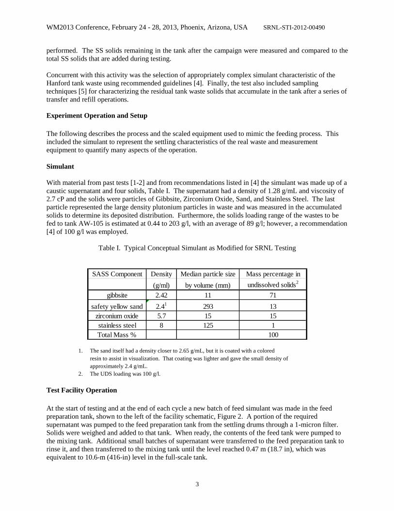
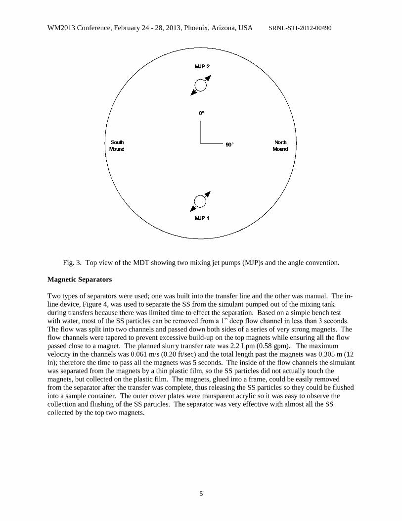
The mixing tank was then mixed and partially fluidized by two jet pumps rotating in a clockwise direction

and synchronized such that the jets from the two pumps remained parallel to each other, Figure 3. When

ready a batch transfer was pumped from the mixing tank through a magnetic separator, to one of the

seven receipt tanks. The elevations of the top of the settled solids and the interface between the white

Gibbsite/zirconium oxide solids and the yellow sand were measured in each tank to provide estimates of

the volumes transferred to each tank. After all the receipt tanks were full the contents of those tanks were

transferred to the settling drums to reuse the liquid portion of the simulant on the following day. During

each cycle, and after each batch transfer, the SS captured in the magnetic separator was collected. Later

those samples were washed to remove dissolved solids and any entrained non-magnetic, and then dried

and weighed.

Fig. 2. The Schematic of the Mixing Demonstration Tank Facility.

Once the heel level was reached the cycle was complete and that transfer was stopped. At the end of the

1st, 5

th, and 10

th cycles heel measurements were made to evaluate the mounds of accumulated solids with

measurement techniques that will be described later. These measurements began by slowly draining the

heel liquid, while providing some agitation. When drained, the tank bottom, in the areas of the mounds,

was mapped with a laser system. When the mapping sequence was complete the laser positioning system

was used to position the core sampler draw cores from each of the two mounds of solids. Once core

sampling was complete the MDT was slowly refilled with the supernatant portion of the removed heel

material in 0.0051-m (0.2-in) increments. At each increment pictures of each of the mounds were taken

to develop topographical maps of the accumulated solids. Once both mounds were covered the remaining

removed heel material was mixed and pumped to the mixing tank to fully re-establish the heel. The heel

measurement process was then complete and the MDT was ready to be fully refilled to begin the next

cycle.

Feed

Prep.

Tank

Solids Settling Tanks

Recovered Liquid Transport Tube

SolidsReceipt Tank 1

Sol idsReceipt Tank 7 {for partial batch}

Solids

Feed

JetPum p

JetPum p

Ma gnet ic Se parat or for Stain less Stee l Particles






Fil ter to remo ve sma ll pa rticl es

Mixing Demonstration Tank


5

Fig. 3. Top view of the MDT showing two mixing jet pumps (MJP)s and the angle convention.

Magnetic Separators

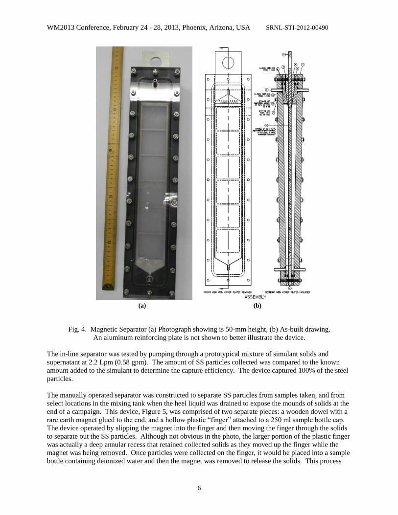
Two types of separators were used; one was built into the transfer line and the other was manual. The in-

line device, Figure 4, was used to separate the SS from the simulant pumped out of the mixing tank

during transfers because there was limited time to effect the separation. Based on a simple bench test

with water, most of the SS particles can be removed from a 1” deep flow channel in less than 3 seconds.

The flow was split into two channels and passed down both sides of a series of very strong magnets. The

flow channels were tapered to prevent excessive build-up on the top magnets while ensuring all the flow

passed close to a magnet. The planned slurry transfer rate was 2.2 Lpm (0.58 gpm). The maximum

velocity in the channels was 0.061 m/s (0.20 ft/sec) and the total length past the magnets was 0.305 m (12

in); therefore the time to pass all the magnets was 5 seconds. The inside of the flow channels the simulant

was separated from the magnets by a thin plastic film, so the SS particles did not actually touch the

magnets, but collected on the plastic film. The magnets, glued into a frame, could be easily removed

from the separator after the transfer was complete, thus releasing the SS particles so they could be flushed

into a sample container. The outer cover plates were transparent acrylic so it was easy to observe the

collection and flushing of the SS particles. The separator was very effective with almost all the SS

collected by the top two magnets.


6

(a) (b)

Fig. 4. Magnetic Separator (a) Photograph showing is 50-mm height, (b) As-built drawing.

An aluminum reinforcing plate is not shown to better illustrate the device.

The in-line separator was tested by pumping through a prototypical mixture of simulant solids and

supernatant at 2.2 Lpm (0.58 gpm). The amount of SS particles collected was compared to the known

amount added to the simulant to determine the capture efficiency. The device captured 100% of the steel

particles.

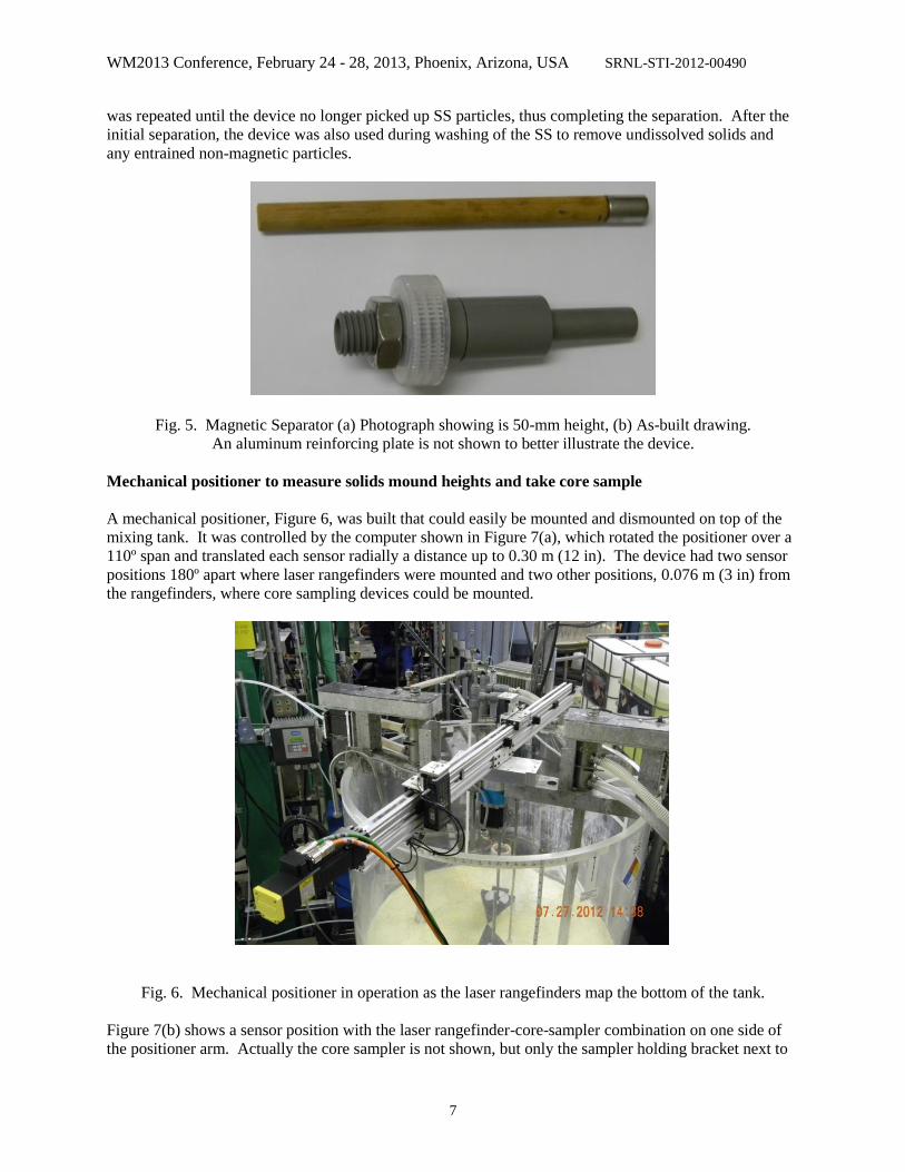
The manually operated separator was constructed to separate SS particles from samples taken, and from

select locations in the mixing tank when the heel liquid was drained to expose the mounds of solids at the

end of a campaign. This device, Figure 5, was comprised of two separate pieces: a wooden dowel with a

rare earth magnet glued to the end, and a hollow plastic “finger” attached to a 250 ml sample bottle cap.

The device operated by slipping the magnet into the finger and then moving the finger through the solids

to separate out the SS particles. Although not obvious in the photo, the larger portion of the plastic finger

was actually a deep annular recess that retained collected solids as they moved up the finger while the

magnet was being removed. Once particles were collected on the finger, it would be placed into a sample

bottle containing deionized water and then the magnet was removed to release the solids. This process


7

was repeated until the device no longer picked up SS particles, thus completing the separation. After the

initial separation, the device was also used during washing of the SS to remove undissolved solids and

any entrained non-magnetic particles.

Fig. 5. Magnetic Separator (a) Photograph showing is 50-mm height, (b) As-built drawing.

An aluminum reinforcing plate is not shown to better illustrate the device.

Mechanical positioner to measure solids mound heights and take core sample

A mechanical positioner, Figure 6, was built that could easily be mounted and dismounted on top of the

mixing tank. It was controlled by the computer shown in Figure 7(a), which rotated the positioner over a

110º span and translated each sensor radially a distance up to 0.30 m (12 in). The device had two sensor

positions 180º apart where laser rangefinders were mounted and two other positions, 0.076 m (3 in) from

the rangefinders, where core sampling devices could be mounted.

Fig. 6. Mechanical positioner in operation as the laser rangefinders map the bottom of the tank.

Figure 7(b) shows a sensor position with the laser rangefinder-core-sampler combination on one side of

the positioner arm. Actually the core sampler is not shown, but only the sampler holding bracket next to


8

the rangefinder. The laser rangefinders move in tandem and as one rangefinder moved further from one

side of the mixing tank wall the other rangefinder moved closer to the opposite wall.

(a) (b)

Fig. 7. Operation of the laser system: (a) System was driven by a computer, (b) and made height

measurements with a laser rangefinder – the core sampler fit in the slotted bracket shown next to the

rangefinder.

To measure solids mounds the positioner was set at 0º and 0-meter (0-in) translation2. Height

measurements were made by both rangefinders simultaneously and after each measurement the positioner

was translated 0.019 m (0.75 in). At the end of a series of height measurements, along a single angle, the

positioner was returned to the 0-meter (0-in) translation location and then the positioner was rotated 2.5º.

The process would then repeat until reaching 110º-rotation position when a total of 1400 measurements

were taken.

Before installation on the positioner the two lasers to be used were calibrated for distance to ±0.0010 m

(±0.04 in). Once the lasers were installed the positions on the tank bottom were calibrated with a map of

the laser measurement positions that was placed in the mixing tank. The laser positions were checked and

the positional accuracy was estimated at ±0.0048 m (±0.19 in).

Measurement of Accumulated Solids Volume by Laser and with Photographs

The process of obtaining volume from laser data began by adding 0.0762 m (3 in) to the average distance

measured to the tops of the two 0.0762-m tall black arrowhead-shaped indicator platforms, thereby

obtaining an accurate distance measure from the laser to the tank bottom. (Note, these platforms, one of

which is shown in Figure 8 were placed in the MDT after the heel material was drained.) They served to

verify laser heights, because they were exactly 0.0762 m above the tank bottom, and had a scale that was

manually set during the photographic technique so the liquid level was recorded. For example, Figure 8

shows the platform indicating 02 which meant a height of 0.0051 m (0.2 in) of liquid. The letter S shown

on the platform indicated the South Mound, refer to Figure 3 for the tank orientation. The width of the

platform was exactly 6” to provide a known, fixed dimension, reference to ensure all photos of the

contour lines could be scaled properly.

2 For the positioner its 0° point was 47° from the MJP centerline, see Figure 3, and the full 110° rotation was from

47° to 157° to scan one mound and 227° to 337° to scan the opposite mound.


9

Fig.8. Triangular platform that stood 0.0762 m (3 in) off tank bottom. It also indicated which mound,

e.g., S=South, and the tank level by manually setting indicator.

To calculate mound volume, a trapezoidal area was associated with each laser measurement point. Every

height measurement was multiplied by its associated area to give an increment of volume. Increments of

volume were added to give total mound volume, Eq. (1).

∑ (Eq. 1)

To estimate the measurement uncertainty for the laser scan of the solids mounds both sand mounds and

objects of known volume were placed in the tank, e.g., Figure 9. Table II shows an aluminum block was

measured to ±9%; however, because the block had straight sides and the laser positions were every 0.019

m (0.75 in) and 2.5°, this large uncertainty was not surprising. Furthermore, the measured volumes of the

sand mounds depend on the packing density, so once again the range of measurement error obtained, i.e.,

±1.9 to ±8% was not surprising. The large plastic mound shown in Figure 9 gives a better representation

of the measurement uncertainty because it was large and smooth. However, the ±0.3% obtained with the

plastic mound is believed much better than can be reasonably expected during actual measurement of real

mounds because it was much bigger and wider than the actual mounds obtained. The measurement

uncertainty was estimated from the average for the two sand mounds, or ±5%. The uncertainty may be

better than the estimate, but more time would be necessary to determine this fact.


10

Fig. 9. Determining volumes in the MDT with the laser using known volumes. Laser was not placed on

the tank yet in the picture.

Table II. Trial volumes for the laser to measure.

Volume by Photographs

Each photographic image included one of the black plastic indicator platforms labeled N or S to designate

which mound, Figure 8. While the series of photographs was taken of each mound the platforms were not

moved to allow later alignment of those images. A pointer on each platform showed the tank level for the

photograph and was manually increased to correspond to the increasing tank level. Furthermore, as the

tank level increased the mounds formed islands of decreasing area. From the photographs each image

was traced to follow shoreline of the islands after which the photographs were resized so that image of the

black platform was the same length in each. The area inside the shoreline was determined for each

Known Laser Difference

Date Test Item of Volumes Measure from Known

Know Volume m3

m3

Percent

5/15/2012 Sand Mound 0.00613 0.00601 1.9%

6/21/2012 Aluminum Block 0.00107 0.00097 8.8%

7/11/2012 Plastic Mound 0.00585 0.00587 0.3%

7/11/2012 Sand Mound 0.00200 0.00184 8.0%


11

photograph and scaled by the known dimensions of the black plastic platform. The result for each mound

was a list of areas and associated elevations (tank heights). The first method used to integrate the data to

yield volume was the Simpson’s Rule [13], Eq. (2).

∑ (Eq. 2)

Simpson’s Rule worked well in a test using sand and water when performing the trial test for the

photographic/volume technique with a mock mound shown in Figure 10.

Fig. 10. Yellow sand mound in water to determine contrast between liquid and solids and estimate

measurement uncertainty.

Photographs were taken at nine fixed liquid levels, e.g., Figure 10 is at 0.02 m (0.8 in). For each

photograph the shoreline between the island and the water was visually determined and manually

superimposed on a drawing. The horizontal area of each elevation was measured and volume was

computed as the integral of area with respect to elevation. In using the Simpson’s rule the resulting

volume was 1.23 x 10-6

m3 (20.1 in

3), which is within 3% of the volume of sand originally added.

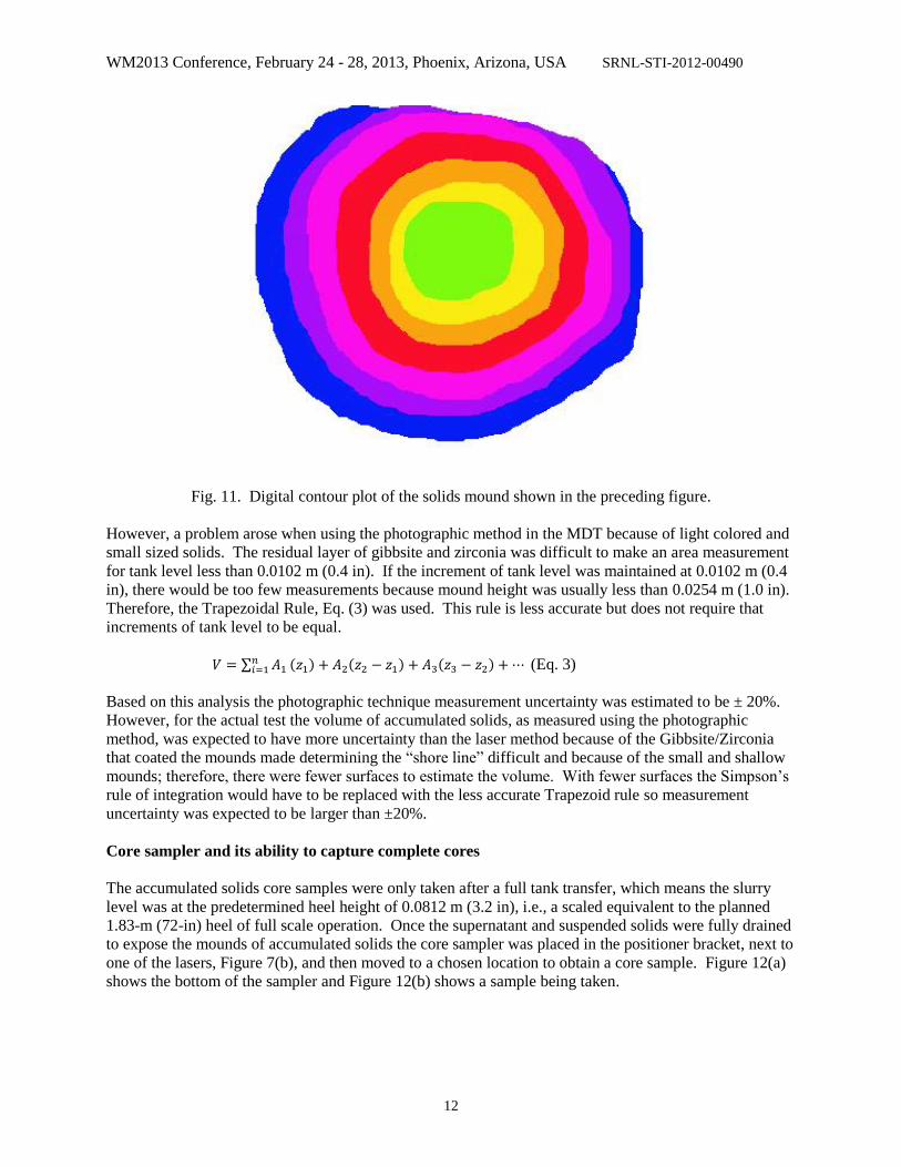
Unfortunately, the care and time necessary to perform this measurement by hand was prohibitive. A more

practical method was to use digital images of the photographs, Figure 11, and from this process the

volume was estimated at 1.32 x 10-6

m3 (21.6 in

3), or within 11% of the known volume. However, this is

an ideal case, under controlled conditions, and the measurement uncertainty for the actual mounds was

expected to be higher.

Shore Line


12

Fig. 11. Digital contour plot of the solids mound shown in the preceding figure.

However, a problem arose when using the photographic method in the MDT because of light colored and

small sized solids. The residual layer of gibbsite and zirconia was difficult to make an area measurement

for tank level less than 0.0102 m (0.4 in). If the increment of tank level was maintained at 0.0102 m (0.4

in), there would be too few measurements because mound height was usually less than 0.0254 m (1.0 in).

Therefore, the Trapezoidal Rule, Eq. (3) was used. This rule is less accurate but does not require that

increments of tank level to be equal.

∑ ( ) ( ) ( ) (Eq. 3)

Based on this analysis the photographic technique measurement uncertainty was estimated to be ± 20%.

However, for the actual test the volume of accumulated solids, as measured using the photographic

method, was expected to have more uncertainty than the laser method because of the Gibbsite/Zirconia

that coated the mounds made determining the “shore line” difficult and because of the small and shallow

mounds; therefore, there were fewer surfaces to estimate the volume. With fewer surfaces the Simpson’s

rule of integration would have to be replaced with the less accurate Trapezoid rule so measurement

uncertainty was expected to be larger than ±20%.

Core sampler and its ability to capture complete cores

The accumulated solids core samples were only taken after a full tank transfer, which means the slurry

level was at the predetermined heel height of 0.0812 m (3.2 in), i.e., a scaled equivalent to the planned

1.83-m (72-in) heel of full scale operation. Once the supernatant and suspended solids were fully drained

to expose the mounds of accumulated solids the core sampler was placed in the positioner bracket, next to

one of the lasers, Figure 7(b), and then moved to a chosen location to obtain a core sample. Figure 12(a)

shows the bottom of the sampler and Figure 12(b) shows a sample being taken.


13

(a) (b)

Fig. 12. Core Sampling: (a) The core end of the sampler, (b) a core extracted during Cycle 1.

The concept that was developed uses the a “finger over the straw” technique, that is, pushing a thin-wall

tube into the heel mound, and then sealing off the top of the tube to lift the captured core sample out of

the mound. Of course, implementing this simple process without disturbing the mound significantly and

doing it at the desired location requires a more sophisticated technique. The core sample incorporates a

thin wall outer tube with an O-ring sealed plug where the tube and seal can move relative to each other.

Withdrawing a complete sample was facilitated by pressing down on the plug to pack the solids slightly

and force out liquid prior to removing the sampler. As can be seen in Figure 12(b) in most cases the

overlying solids on the mound, assumed to be mostly gibbsite, tends to back fill the hole as soon as the

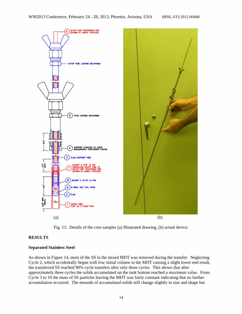
core sampler removes a plug. Figure 13 shows the entire core sampler and the drawing used to construct

the device and the accuracy of the placement of the sampler was estimated at ±0.0095 m (±3/8 in).


14

(a) (b)

Fig. 13. Details of the core sampler (a) Illustrated drawing, (b) actual device.

RESULTS

Separated Stainless Steel

As shown in Figure 14, most of the SS in the mixed MDT was removed during the transfer. Neglecting

Cycle 2, which accidentally began with low initial volume in the MDT causing a slight lower end result,

the transferred SS reached 90% cycle transfers after only three cycles. This shows that after

approximately three cycles the solids accumulated on the tank bottom reached a maximum value. From

Cycle 3 to 10 the mass of SS particles leaving the MDT was fairly constant indicating that no further

accumulation occurred. The mounds of accumulated solids still change slightly in size and shape but


15

there does not appear to be further growth, as will be seen from the photographic evidence shown in the

next section. On the average 88% the cycle-to-cycle charge of SS solids transferred out of the mixing

tank over the entire campaign.

Fig. 14. Stainless steel transfer during the campaign

Mound Volumes – Laser Method

The mounds are displayed both photographically (Figures 15 and 16) and graphically (Figures 17-20).

The test included the evaluation of many mounds of solids and these figures are examples of the

measured results. The results after Cycles 1, 5 and 10 are shown in Figure 21 with a measurement

uncertainty of ±5%. The photographs of the mounds are shown to better understand the actual size of the

North and South mounds. To see the quantitative size of the mounds the scale of the laser data was

expanded, which make the mounds look much larger than they were. Furthermore, for each mound in

each cycle there are two laser measurement views: First, a side view, which has the perspective of

looking at the mound from the center of the tank, and second, a top view of same mound.

50%

60%

70%

80%

90%

100%

1 2 3 4 5 6 7 8 9 10

Sta

inle

ss S

teel

, %

Cycle Number

Total SS per Cycle: 392 gram

Average Cycle SS Transfer : 88%

Initial MDT volume was low


16

Fig. 15. Solids North mound after Cycle 10 and after core samples were taken.

Fig. 16. Solids South mound after Cycle 10 and after core samples were taken.


17

Fig. 17. North Mound side view after Cycle 10 – Volume of 58.0 x 10-5

m3 (35.4 in

3).

Fig. 18. North Mound top view after Cycle 10 – Volume of 58.0 x 10-5

m3 (35.4 in

3).


18

Fig. 19. South Mound side view after Cycle 10 – Volume of 15.1 x 10-5

m3 (9.2 in

3).

Fig. 20. South Mound top view after Cycle 10 – Volume of 15.1 x 10

-5 m

3 (9.2 in

3).


19

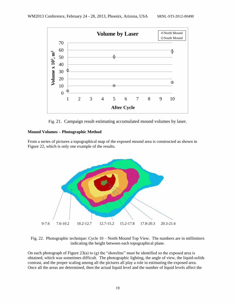
Fig. 21. Campaign result estimating accumulated mound volumes by laser.

Mound Volumes – Photographic Method

From a series of pictures a topographical map of the exposed mound area is constructed as shown in

Figure 22, which is only one example of the results.

Fig. 22. Photographic technique: Cycle 10 – North Mound Top View. The numbers are in millimiters

indicating the height between each topographical plane.

On each photograph of Figure 23(a) to (g) the “shoreline” must be identified so the exposed area is

obtained, which was sometimes difficult. The photographic lighting, the angle of view, the liquid-solids

contrast, and the proper scaling among all the pictures all play a role in estimating the exposed area.

Once all the areas are determined, then the actual liquid level and the number of liquid levels affect the

0

10

20

30

40

50

60

70

1 2 3 4 5 6 7 8 9 10

Vo

lum

e x

10

5, m

3

After Cycle

Volume by Laser North Mound

South Mound

0-7.6 7.6-10.2 10.2-12.7 12.7-15.2 15.2-17.8 17.8-20.3 20.3-21.6


20

accuracy, which increases as the number of levels increases. For the North Mound depicted in Figure 23

it had seven levels, because it was about 22 mm tall.

(a) 0.0 mm tank level (b) 7.6 mm tank level

(c) 10.2 mm tank level (d) 12.7 mm tank level

(e) 15.2 mm tank level (f) 17.8 mm tank level


21

\

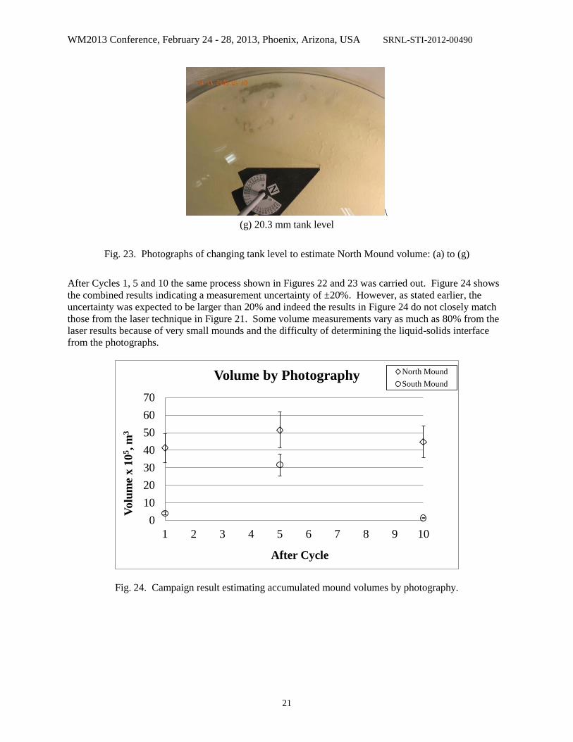
(g) 20.3 mm tank level

Fig. 23. Photographs of changing tank level to estimate North Mound volume: (a) to (g)

After Cycles 1, 5 and 10 the same process shown in Figures 22 and 23 was carried out. Figure 24 shows

the combined results indicating a measurement uncertainty of ±20%. However, as stated earlier, the

uncertainty was expected to be larger than 20% and indeed the results in Figure 24 do not closely match

those from the laser technique in Figure 21. Some volume measurements vary as much as 80% from the

laser results because of very small mounds and the difficulty of determining the liquid-solids interface

from the photographs.

Fig. 24. Campaign result estimating accumulated mound volumes by photography.

0

10

20

30

40

50

60

70

1 2 3 4 5 6 7 8 9 10

Vo

lum

e x 1

05, m

3

After Cycle

Volume by Photography North Mound

South Mound


22

Core Samples

As can be seen from Figures 15, 16, and 23 core sample were taken as part of the heel measurements and

the core sampler did a good job of extracting cores, as seen in Figure 25.

(a) (b)

Fig. 25. Core samples; a) Cycle 5 sample (bottom is to the right side, and b) Cycle 10 sample (bottom is

to the left side), taken from the North Mound.

For the entire campaign 23 core samples were taken. Some of the samples were long enough to divide

into sections in order to measure the concentration of SS at different height. However, because the

samples were small the best that can be stated is that the SS was found primarily on the bottom sections

of the cores, while the top sections had less SS and more of the other solids, i.e., primarily sand, but some

gibbsite and zirconia, too.

Remaining Tank Material

After all campaign cycles were completed the residual solids left in the mixing tank were measured for

SS. Using the hand-held magnet, Figure 5, the SS from each mound was removed separately, and then

the SS from the remaining solids was collected. The results are shown in Table III.

Table III. Stainless steel (SS) left in mixing tank after campaign was complete

As was shown from the laser results the volume of the North Mound was approximately 4 times larger

than the South Mound, e.g., see Figures 17, 19, and 21. The collected SS from the mounds follows this

trend, i.e., 75/18 ~4, which is consistent and indicate the estimate to be fairly accurate.

Grams of SS % Total Location

182.9 75% North Mound

44.1 18% South Mound

17.5 7% All Other Areas

244.5 100% Total Heel


23

CONCLUSIONS

More than 85% of very fast settling particles, i.e., ~125 m SS, transported out of the mixing tank,

but did accumulate until about the 3rd

cycle, after which more than 90% of the SS solids introduced

into the tanks were transported out.

Solids did accumulate in the two “dead zones” of the tank, i.e., the locations opposite of the jet pump

mixers and accumulations occurred almost immediate on mixing the tank, i.e., before transfer began.

The mounds of solids that formed, referred to as the North and South Mounds, were of unequal size

with the North Mound approximately four times the volume of the South Mound. This volume

difference was due to the different strengths for the two mixing jet pump velocities.

Accumulated volumes determined by the two methods employed, i.e., laser and photographic, agreed

on the average to within 22% for the North Mound and 83% for the South Mound. This measurement

difference was not unexpected because the mounds were small, less than 25 mm in height for the

North Mounds and less than 13 mm in height for the South Mounds. Furthermore, the small sized

solids, i.e., gibbsite and zirconia, covered everything making the contrast between the supernatant and

solids difficult for the photographic technique to clearly distinguish the liquid-solids interfaces. [The

smaller the volume and the poorer surface contrast the more measurement uncertainty for the

photographic technique.]

Core samples taken from the mounds clearly indicated that SS is the predominant component of the

bottom of the settled volumes. The composition gradually transitions to sand in the upper surface of

the mounds.

At the end of 10 cycles the amount of SS that remained in the staging tank was 7.4% of the total used,

i.e., 244.5 grams in heel of the 3308 grams put into the mixing tank.

93% of the residual SS was shown to be located within the mounds of accumulated solids with the

remaining 7% in all other locations.

Further details on the results and measurement techniques can be found in Ref. [10].

ACKNOWLEDGMENT

The U.S. Department of Energy supported this work through contract no. DE-A-AC09-08SR22470.

REFERENCES

1. D. J. ADAMSON, M. R. POIRER, and T. J. STEEPER, “Demonstration of Simulated Waste

Transfers from Tank AY-102 to the Hanford Waste Treatment Facility,” SRNL-STI-2009-00717,

Rev. 0 (2009)

2. D. J. ADAMSON, M. L. RESTIVO, T. J. STEEPER, and D. A. GREER, “Demonstration of Mixer

Jet Pump Rotational Sensitivity on Mixing and Transfers of the AY-102 Tank,” SRNL-STI-2010-

00521, Rev. 0 (2010).

3. D. J. ADAMSON and P. A. GAUGLITZ, “Demonstration of Mixer and Transferring Settling

Cohesive Slurry Simulants in the AY-102 Tank,” SRNL-STI-2011-00278, Rev. 0. (2011).

4. K. P. LEE, B. E. WELLS, P. A. GAUGLITZ, and R.A. SEXTON, “Waste Feed Delivery Mixing

and Sampling Program Simulant Definition for Tank Farm Performance Testing,” RPP-PLAN-

51625, Rev.0 (2012).

5. M. R. DUIGNAN, T. J. STEEPER, J. L. STEIMKE, and M. D. FOWLEY, “Simulant Development

and Sampling Plan,” SRNL-L3100-2012-00024 (2012).

6. “Interface Control Document for Waste Feed,” 24590-WTP-ICD-MG-01-019, Rev. 5 Bechtel

National, Inc. Richland, Washington (2011).


24

7. D. L. HERTING, to E. A. NELSON, “Preparation of Simulated SST Early Feed Solution for Pilot

Plant,” CH2M-0701541 (2007)

8. M. R. DUIGNAN, T. J. STEEPER, J. L. STEIMKE, and M. D. FOWLEY, “Test Plan – Solids

Accumulation Scouting Studies,” SRNL-STI-2012-00239, Rev. 0 (2012).

9. W. KAPLAN, W., Advanced Calculus, p. 171, Addison-Wesley Pub. Co. (1952).\

10. M. R. DUIGNAN, T. J. STEEPER, and J. L. STEIMKE, “Solids Accumulation Scoping Studies,”

SRNL-STI-2012-00508, Rev. 0 (2012).

Documents

Experimental Methods to Estimate Accumulated Solids … · WM2013 Conference, February 24 - 28, 2013, Phoenix, Arizona, USA SRNL-STI-2012-00490 1 Experimental Methods to Estimate