Experimental modal analysis of the tyre measurement tower

Citation for published version (APA):Schrijver, de, P. A. R. (2005). Experimental modal analysis of the tyre measurement tower. (DCT rapporten; Vol.2005.112). Technische Universiteit Eindhoven.

Document status and date:Published: 01/01/2005

Document Version:Publisher’s PDF, also known as Version of Record (includes final page, issue and volume numbers)

Please check the document version of this publication:

• A submitted manuscript is the version of the article upon submission and before peer-review. There can beimportant differences between the submitted version and the official published version of record. Peopleinterested in the research are advised to contact the author for the final version of the publication, or visit theDOI to the publisher's website.• The final author version and the galley proof are versions of the publication after peer review.• The final published version features the final layout of the paper including the volume, issue and pagenumbers.Link to publication

General rightsCopyright and moral rights for the publications made accessible in the public portal are retained by the authors and/or other copyright ownersand it is a condition of accessing publications that users recognise and abide by the legal requirements associated with these rights.

• Users may download and print one copy of any publication from the public portal for the purpose of private study or research. • You may not further distribute the material or use it for any profit-making activity or commercial gain • You may freely distribute the URL identifying the publication in the public portal.

If the publication is distributed under the terms of Article 25fa of the Dutch Copyright Act, indicated by the “Taverne” license above, pleasefollow below link for the End User Agreement:www.tue.nl/taverne

Take down policyIf you believe that this document breaches copyright please contact us at:openaccess@tue.nlproviding details and we will investigate your claim.

Download date: 12. Dec. 2021

Experimental modal analysis ofthe tyre measurement tower

P.A.R. de Schrijver

DCT 2005.112

Traineeship report

Coach(es): Dr. Ir. A.J.C. SchmeitzDr. Ir. I. Lopez Arteaga

Supervisor: Prof. Dr. Ir. H. Nijmeijer

Technische Universiteit EindhovenDepartment Mechanical EngineeringDynamics and Control Technology Group

Eindhoven, August, 2005

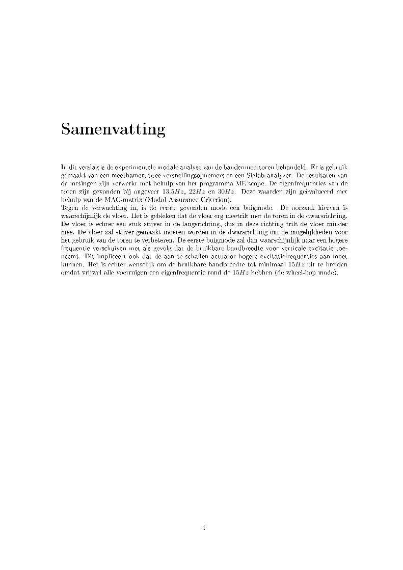
Samenvatting

In dit verslag is de experimentele modale analyse van de bandenmeettoren behandeld. Er is gebruikgemaakt van een meethamer, twee versnellingsopnemers en een Siglab-analyzer. De resultaten vande metingen zijn verwerkt met behulp van het programma ME'scope. De eigenfrequenties van detoren zijn gevonden bij ongeveer 13.5Hz, 22Hz en 30Hz. Deze waarden zijn geëvalueerd metbehulp van de MAC-matrix (Modal Assurance Criterion).Tegen de verwachting in, is de eerste gevonden mode een buigmode. De oorzaak hiervan iswaarschijnlijk de vloer. Het is gebleken dat de vloer erg meetrilt met de toren in de dwarsrichting.De vloer is echter een stuk stijver in de langsrichting, dus in deze richting trilt de vloer mindermee. De vloer zal stijver gemaakt moeten worden in de dwarsrichting om de mogelijkheden voorhet gebruik van de toren te verbeteren. De eerste buigmode zal dan waarschijnlijk naar een hogerefrequentie verschuiven met als gevolg dat de bruikbare bandbreedte voor verticale excitatie toe-neemt. Dit impliceert ook dat de aan te scha�en actuator hogere excitatiefrequenties aan moetkunnen. Het is echter wenselijk om de bruikbare bandbreedte tot minimaal 15Hz uit te breidenomdat vrijwel alle voertuigen een eigenfrequentie rond de 15Hz hebben (de wheel-hop mode).

i

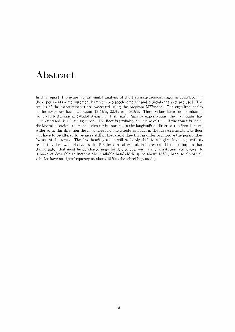
Abstract

In this report, the experimental modal analysis of the tyre measurement tower is described. Inthe experiments a measurement hammer, two accelerometers and a Siglab-analyzer are used. Theresults of the measurements are processed using the program ME'scope. The eigenfrequenciesof the tower are found at about 13.5Hz, 22Hz and 30Hz. These values have been evaluatedusing the MAC-matrix (Modal Assurance Criterion). Against expectations, the �rst mode thatis encountered, is a bending mode. The �oor is probably the cause of this. If the tower is hit inthe lateral direction, the �oor is also set in motion. In the longitudinal direction the �oor is muchsti�er so in this direction the �oor does not participate as much in the measurements. The �oorwill have to be altered to be more sti� in the lateral direction in order to improve the possibilitiesfor use of the tower. The �rst bending mode will probably shift to a higher frequency with asresult that the available bandwidth for the vertical excitation increases. This also implies thatthe actuator that must be purchased must be able to deal with higher excitation frequencies. Itis however desirable to increase the available bandwidth up to about 15Hz, because almost allvehicles have an eigenfrequency at about 15Hz (the wheel-hop mode).

ii

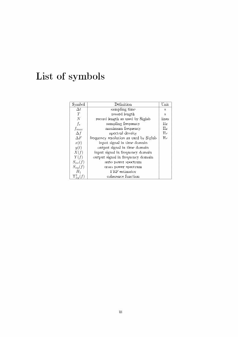
List of symbols

Symbol De�nition Unit∆t sampling time sT record length sN record length as used by Siglab linesfs sampling frequency Hz

fmax maximum frequency Hz∆f spectral density Hz∆F frequency resolution as used by Siglab Hzx(t) input signal in time domainy(t) output signal in time domainX(f) input signal in frequency domainY (f) output signal in frequency domain

Sxx(f) auto power spectrumSxy(f) cross power spectrum

H1 FRF estimatorΥ2

xy(f) coherence function

iii

Contents

Samenvatting . . . . . . . . . . . . . . . . . . . . . . . . . . . . . . . . . . . . . . . . . . iAbstract . . . . . . . . . . . . . . . . . . . . . . . . . . . . . . . . . . . . . . . . . . . . . iiList of symbols . . . . . . . . . . . . . . . . . . . . . . . . . . . . . . . . . . . . . . . . . iii

1 Introduction 11.1 The measurement tower . . . . . . . . . . . . . . . . . . . . . . . . . . . . . . . . . 11.2 The role of modal analysis . . . . . . . . . . . . . . . . . . . . . . . . . . . . . . . . 21.3 Goals and report structure . . . . . . . . . . . . . . . . . . . . . . . . . . . . . . . . 2

2 Experiments 32.1 Method and experimental setup . . . . . . . . . . . . . . . . . . . . . . . . . . . . . 3

2.1.1 Measuring equipment . . . . . . . . . . . . . . . . . . . . . . . . . . . . . . 42.1.2 The measurement Points . . . . . . . . . . . . . . . . . . . . . . . . . . . . . 6

2.2 The measurements . . . . . . . . . . . . . . . . . . . . . . . . . . . . . . . . . . . . 62.2.1 Input range . . . . . . . . . . . . . . . . . . . . . . . . . . . . . . . . . . . . 72.2.2 Frequency range . . . . . . . . . . . . . . . . . . . . . . . . . . . . . . . . . 72.2.3 Triggering . . . . . . . . . . . . . . . . . . . . . . . . . . . . . . . . . . . . . 82.2.4 Windowing . . . . . . . . . . . . . . . . . . . . . . . . . . . . . . . . . . . . 82.2.5 Averaging . . . . . . . . . . . . . . . . . . . . . . . . . . . . . . . . . . . . . 82.2.6 Frequency response functions . . . . . . . . . . . . . . . . . . . . . . . . . . 9

3 Modal parameter estimation 103.1 Number of modes . . . . . . . . . . . . . . . . . . . . . . . . . . . . . . . . . . . . . 103.2 Modal parameter estimation method . . . . . . . . . . . . . . . . . . . . . . . . . . 123.3 The estimates . . . . . . . . . . . . . . . . . . . . . . . . . . . . . . . . . . . . . . . 12

4 Evaluation 144.1 Evaluation of the measurements . . . . . . . . . . . . . . . . . . . . . . . . . . . . . 144.2 The mode shapes . . . . . . . . . . . . . . . . . . . . . . . . . . . . . . . . . . . . . 154.3 MAC values . . . . . . . . . . . . . . . . . . . . . . . . . . . . . . . . . . . . . . . . 164.4 Discussion . . . . . . . . . . . . . . . . . . . . . . . . . . . . . . . . . . . . . . . . . 17

5 Conclusions and recommendations 18

A Estimated mode shapes 19

iv

Chapter 1

Introduction

This report is the result of an internship performed at Eindhoven University of Technology. Inthis report, the experimental modal analysis of a tyre measurement tower is described. In thisintroduction �rst the measurement tower itself is discussed. Then the importance of the modalanalysis will be explained and �nally the goals and the structure of this report are discussed.

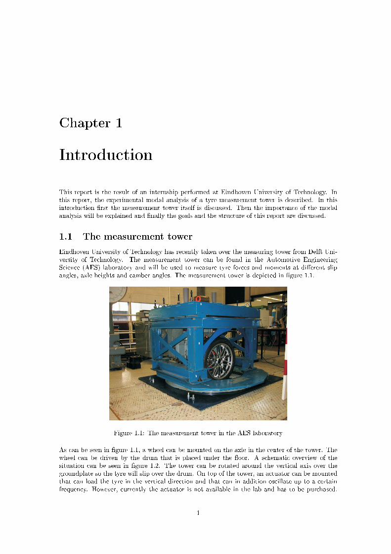
1.1 The measurement towerEindhoven University of Technology has recently taken over the measuring tower from Delft Uni-versity of Technology. The measurement tower can be found in the Automotive EngineeringScience (AES) laboratory and will be used to measure tyre forces and moments at di�erent slipangles, axle heights and camber angles. The measurement tower is depicted in �gure 1.1.

Figure 1.1: The measurement tower in the AES laboratory

As can be seen in �gure 1.1, a wheel can be mounted on the axle in the center of the tower. Thewheel can be driven by the drum that is placed under the �oor. A schematic overview of thesituation can be seen in �gure 1.2. The tower can be rotated around the vertical axis over thegroundplate so the tyre will slip over the drum. On top of the tower, an actuator can be mountedthat can load the tyre in the vertical direction and that can in addition oscillate up to a certainfrequency. However, currently the actuator is not available in the lab and has to be purchased.

1

The prices of di�erent actuators vary a lot because of the di�erent frequency ranges they canhandle. An actuator that can actuate up to 30Hz for instance is much more expensive than onethat can actuate up to 15Hz.

hydropuls

tyre

drumdrum

top frame

wheel frame

measuring hub

bearing

Figure 1.2: Schematic overview of the tower

1.2 The role of modal analysisThe fact that an actuator has to be purchased is the reason that a modal analysis is performed onthe measurement tower. In a modal analysis the dynamic behavior of the tower is investigated.It is important to know the dynamic behavior of the tower in order to make a sensible decisionabout the choice of an actuator.With a modal analysis the modal parameters, modal frequencies, modal damping and the modalshapes are obtained. So after the modal analysis is performed, it is known at what frequenciesthe tower will resonate. The actuator has to be able to actuate at a frequency su�ciently belowthe �rst eigenfrequency of the measurement tower so the measurements are not in�uenced by theresonating tower.

1.3 Goals and report structureThe goal of this report is to determine the modal properties of the tyre measurement tower in theAES lab, so a sensible decision can be made about the choice of an actuator for the measurementtower.The report is organized as follows. In chapter 2 the experiments will be discussed. This includesall the needed equipment, the measurement method and an evaluation of the quality of the mea-surements. In chapter 3 the modal parameters will be determined from the measured data. Inchapter 4 an evaluation of the estimated modal parameters will take place. Finally, in chapter5 some conclusions will be drawn and recommendations will be given for the actuator and forfurther research.

2

Chapter 2

Experiments

In this chapter the experiments performed to obtain the Frequency Response Functions (FRF's) ofthe measurement tower are discussed. First an explanation of the method, setup and the equipmentused for the experiments will be given, then the measurements will be discussed followed by anevaluation of the measurements.

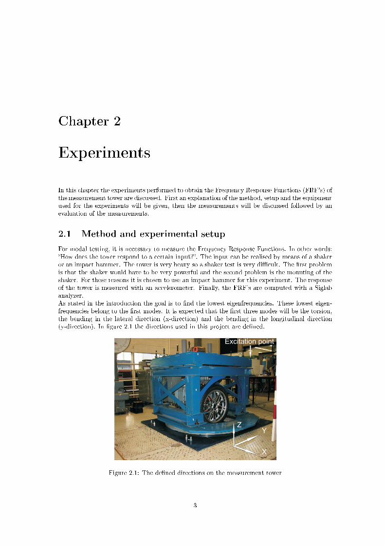
2.1 Method and experimental setupFor modal testing, it is necessary to measure the Frequency Response Functions. In other words:�How does the tower respond to a certain input?�. The input can be realised by means of a shakeror an impact hammer. The tower is very heavy so a shaker test is very di�cult. The �rst problemis that the shaker would have to be very powerful and the second problem is the mounting of theshaker. For these reasons it is chosen to use an impact hammer for this experiment. The responseof the tower is measured with an accelerometer. Finally, the FRF's are computed with a Siglabanalyzer.As stated in the introduction the goal is to �nd the lowest eigenfrequencies. These lowest eigen-frequencies belong to the �rst modes. It is expected that the �rst three modes will be the torsion,the bending in the lateral direction (x-direction) and the bending in the longitudinal direction(y-direction). In �gure 2.1 the directions used in this project are de�ned.

Figure 2.1: The de�ned directions on the measurement tower

3

In order to �nd both the lateral bending and the longitudinal bending, the tower has to be hitin the lateral direction and the longitudinal direction respectively. The torsion mode can befound in both the lateral direction and the longitudinal direction. Due to lack of time the choicehas been made to treat the lateral excitation completely and in the longitudinal direction onlya limited number of points are treated to get an indication of the longitudinal bending. In theexperiment one point was chosen as the �xed hammering point, see �gure 2.1, and the place ofthe accelerometer was changed every measurement. The choice of the di�erent measuring pointswill be discussed later in this section.

2.1.1 Measuring equipmentIn this subsection the measurement equipment will be treated. As mentioned earlier, three piecesof measurement equipment are used: an impact hammer, an accelerometer and a Siglab analyzer.

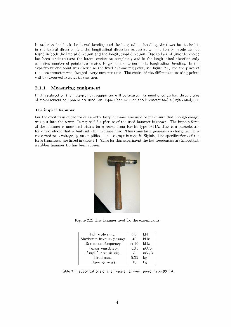
The impact hammerFor the excitation of the tower an extra large hammer was used to make sure that enough energywas put into the tower. In �gure 2.2 a picture of the used hammer is shown. The impact forceof the hammer is measured with a force sensor from Kistler type 9341A. This is a piezoelectricforce transducer that is built into the hammer head. This transducer generates a charge which isconverted to a voltage by an ampli�er. This voltage is used in Siglab. The speci�cations of theforce transducer are listed in table 2.1. Since for this experiment the low frequencies are important,a rubber hammer tip has been chosen.

Figure 2.2: The hammer used for the experiments

Full scale range 30 kNMaximum frequency range 40 kHz

Resonance frequency ≈ 40 kHzSensor sensitivity 4.04 pC/N

Ampli�er sensitivity 5 mV/NHead mass 0.33 kg

Hammer mass 10 kg

Table 2.1: speci�cations of the impact hammer, sensor type 9341A

4

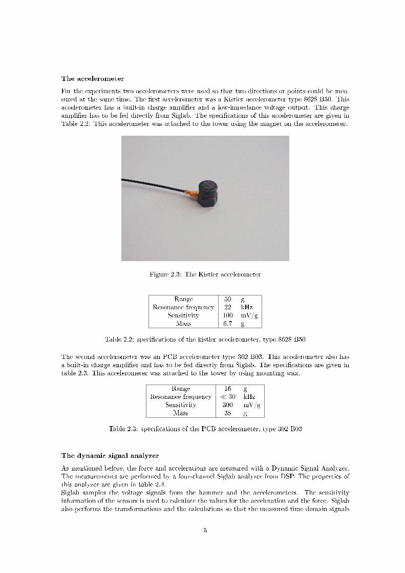
The accelerometerFor the experiments two accelerometers were used so that two directions or points could be mea-sured at the same time. The �rst accelerometer was a Kistler accelerometer type 8628 B50. Thisaccelerometer has a built-in charge ampli�er and a low-impedance voltage output. This chargeampli�er has to be fed directly from Siglab. The speci�cations of this accelerometer are given inTable 2.2. This accelerometer was attached to the tower using the magnet on the accelerometer.

Figure 2.3: The Kistler accelerometer

Range 50 gResonance frequency 22 kHz

Sensitivity 100 mV/gMass 6.7 g

Table 2.2: speci�cations of the kistler accelerometer, type 8628 B50

The second accelerometer was an PCB accelerometer type 302 B03. This accelerometer also hasa built-in charge ampli�er and has to be fed directly from Siglab. The speci�cations are given intable 2.3. This accelerometer was attached to the tower by using mounting wax.

Range 16 gResonance frequency ¿ 30 kHz

Sensitivity 300 mV/gMass 38 g

Table 2.3: speci�cations of the PCB accelerometer, type 302 B03

The dynamic signal analyzerAs mentioned before, the force and accelerations are measured with a Dynamic Signal Analyzer.The measurements are performed by a four-channel Siglab analyzer from DSP. The properties ofthis analyzer are given in table 2.4.Siglab samples the voltage signals from the hammer and the accelerometers. The sensitivityinformation of the sensors is used to calculate the values for the acceleration and the force. Siglabalso performs the transformations and the calculations so that the measured time domain signals

5

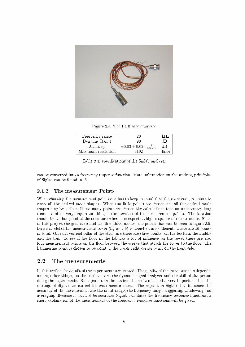
Figure 2.4: The PCB accelerometer

Frequency range 20 kHzDynamic Range 90 dB

Accuracy ±0.03 + 0.02 · f20kHz dB

Maximum resolution 8192 lines

Table 2.4: speci�cations of the Siglab analyzer

can be converted into a frequency response function. More information on the working principlesof Siglab can be found in [6].

2.1.2 The measurement PointsWhen choosing the measurement points one has to keep in mind that there are enough points tocover all the desired mode shapes. When too little points are chosen not all the desired modeshapes may be visible. If too many points are chosen the calculations take an unnecessary longtime. Another very important thing is the location of the measurement points. The locationshould be at that point of the structure where one expects a high response of the structure. Sincein this project the goal is to �nd the �rst three modes, the points that can be seen in �gure 2.5,here a model of the measurement tower (�gure 2.6) is depicted, are su�cient. There are 16 pointsin total. On each vertical pillar of the structure there are three points: on the bottom, the middleand the top. To see if the �oor in the lab has a lot of in�uence on the tower there are alsofour measurement points on the �oor between the screws that attach the tower to the �oor. Thehammering point is chosen to be point 4, the upper right corner point on the front side.

2.2 The measurementsIn this section the details of the experiments are treated. The quality of the measurements depends,among other things, on the used sensors, the dynamic signal analyzer and the skill of the persondoing the experiments. But apart from the devices themselves it is also very important that thesettings of Siglab are correct for each measurement. The aspects in Siglab that in�uence theaccuracy of the measurement are the input range, the frequency range, triggering, windowing andaveraging. Because it can not be seen how Siglab calculates the frequency response functions, ashort explanation of the measurement of the frequency response functions will be given.

6

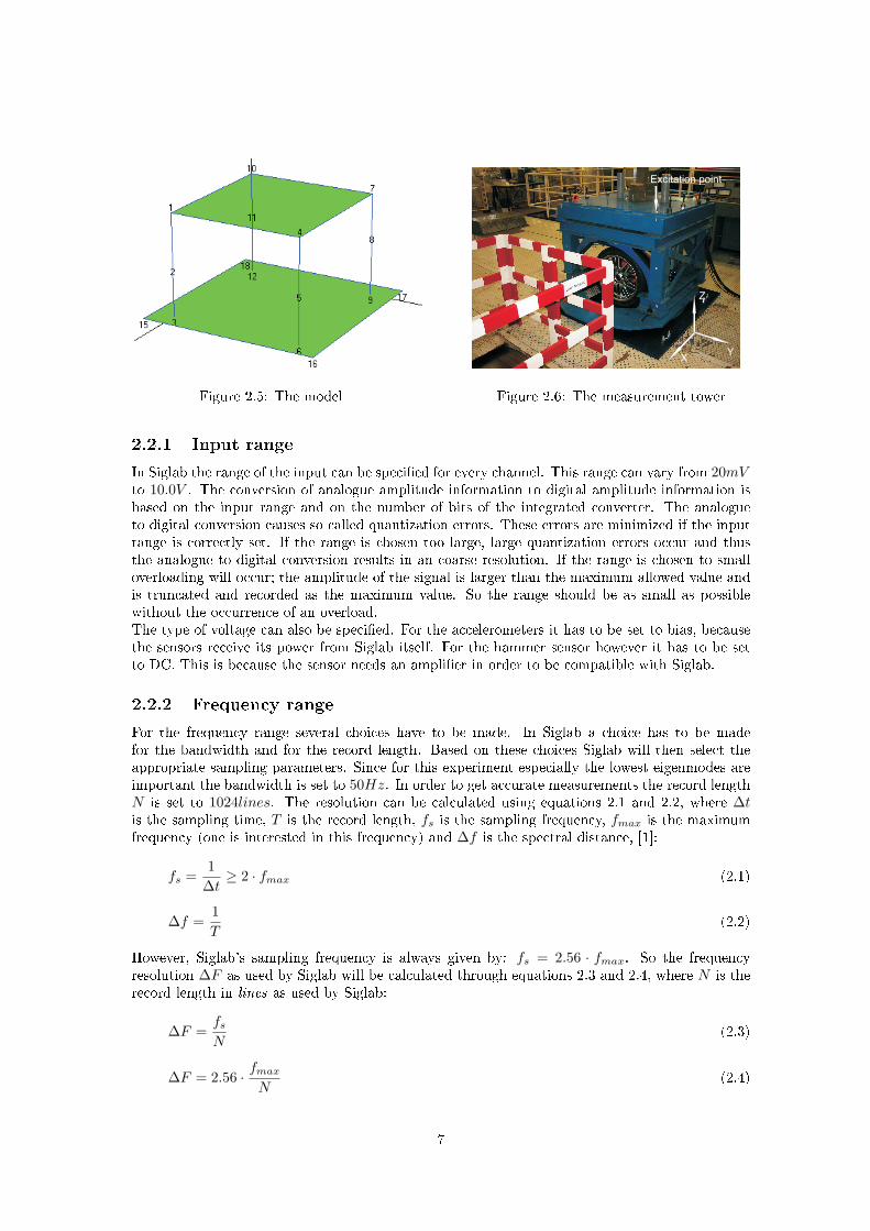
Figure 2.5: The model Figure 2.6: The measurement tower

2.2.1 Input rangeIn Siglab the range of the input can be speci�ed for every channel. This range can vary from 20mVto 10.0V . The conversion of analogue amplitude information to digital amplitude information isbased on the input range and on the number of bits of the integrated converter. The analogueto digital conversion causes so called quantization errors. These errors are minimized if the inputrange is correctly set. If the range is chosen too large, large quantization errors occur and thusthe analogue to digital conversion results in an coarse resolution. If the range is chosen to smalloverloading will occur; the amplitude of the signal is larger than the maximum allowed value andis truncated and recorded as the maximum value. So the range should be as small as possiblewithout the occurrence of an overload.The type of voltage can also be speci�ed. For the accelerometers it has to be set to bias, becausethe sensors receive its power from Siglab itself. For the hammer sensor however it has to be setto DC. This is because the sensor needs an ampli�er in order to be compatible with Siglab.

2.2.2 Frequency rangeFor the frequency range several choices have to be made. In Siglab a choice has to be madefor the bandwidth and for the record length. Based on these choices Siglab will then select theappropriate sampling parameters. Since for this experiment especially the lowest eigenmodes areimportant the bandwidth is set to 50Hz. In order to get accurate measurements the record lengthN is set to 1024lines. The resolution can be calculated using equations 2.1 and 2.2, where ∆tis the sampling time, T is the record length, fs is the sampling frequency, fmax is the maximumfrequency (one is interested in this frequency) and ∆f is the spectral distance, [1]:

fs =1

∆t≥ 2 · fmax (2.1)

∆f =1T

(2.2)

However, Siglab's sampling frequency is always given by: fs = 2.56 · fmax. So the frequencyresolution ∆F as used by Siglab will be calculated through equations 2.3 and 2.4, where N is therecord length in lines as used by Siglab:

∆F =fs

N(2.3)

∆F = 2.56 · fmax

N(2.4)

7

2.2.3 TriggeringTo get good results it is important that the whole excitation signal and the response is captured.This is done by pretriggering the signal. Pretriggering means that the signals are captured beforethe impulse occurs so that the entire signal will be captured. In Siglab three parameters can beset to describe the triggering namely the level, the slope and the pretrigger delay. The level is apercentage of the peakvalue of the total impulse. This determines the amplitude of the signal atwhich the measurements are started. The slope is used to specify if the measurements should bestarted at a growing or decaying signal. These last two parameters tell the measurements to startwhen the impulse is already present so the pretrigger delay is used to ensure that the entire signalis captured. In this project the measurements are triggered at a channel level of 9% at a positiveslope and with a pretrigger delay of −5.0%.

2.2.4 WindowingIn this experiment two time domain windows are used: the force window for the signal from theforce transducer and the exponential window for the accelerometer signal. These windows areapplied to the time signals after they are sampled, but before Siglab calculates the Fast FourierTransform.

The force windowThe impact force signal, measured through the force transducer in the impact hammer, usuallyhas an impulse like form and is very short in time compared to the total measuring time. Afterthe structure is hit by the hammer the force transducer can still give a measurement signal due tonoise, swinging of the hammer, from putting the hammer on the table etcetera. This noise signalnegatively in�uences the measurements so this must be removed somehow. This is the reason touse a force window. The force window is a rectangular window and is used to remove the noisethat is present in the impulse signal. The force window has a value of one in a time band aroundthe impulse signal and is zero elsewhere. In Siglab three parameters can be speci�ed: the doublehit amplitude, the double hit delay time and the force window size. The width of the window isspeci�ed in Siglab as a percentage of the total measuring time. When the structure is accidentallyhit twice, it is called a double hit. In Siglab the double hit is speci�ed as a percentage of the �rsthit. So impulses after the �rst hit with an amplitude larger than this percentage will be rejected.The double hit delay is a percentage of the measuring time. Impulses that occur after the doublehit delay time are also rejected. In this experiment the force window size is set to 10.0%, thedouble hit amplitude is set to 50% and the delay time is set to 20%.

The exponential windowIn the computation of the frequency response functions the Fast Fourier Transformation is used.This transform assumes that the signals are periodic. If the measured signals are not periodicleakage errors will occur. The function of the exponential window is to force the signal to practicallyzero at the end of the sampling window, so the transform can see the signal as periodic with aperiod time as long as the measuring time.In Siglab the exponential window decay can be speci�ed. Here it is set to 1%. This means that atthe end of the sampling window the exponential window is 1% of the beginning value. Althoughthe exponential window reduces leakage errors it also has a disadvantage. It introduces arti�cialdamping to the modes of the structure. In the post processing phase this arti�cial damping canbe removed from the estimated modal damping.

2.2.5 AveragingIn every measurement there can be random errors. These random errors are caused by measure-ment noise and by the person doing the measurements. A way to remove these errors is to do more

8

measurements of the same point and average the results in the frequency domain. This improvesthe accuracy of the measurements. If all the frequency response functions are of equal importancethe averaging can be linear. For this experiment the frequency response functions are measuredusing �ve impacts at the same location. In Siglab there are some other options available. Theseare the double hit reject and the overload reject. Double hit reject means that frames with morethan one impulse are rejected and overload reject means that frames with impacts that exceedsthe measurement ranges are rejected. Furthermore the person doing the measurements can alsomanually reject every frame.

2.2.6 Frequency response functionsThe estimation of the frequency response functions is a process that is performed inside of thefrequency response analyzer and is therefore 'invisible' to the user. In this section the basic ideaof the estimation is presented. More information on the estimation can be found in [1].The input and output signals x(t) and y(t) are measured using a time sampling approach. In orderto transform these signals into the frequency domain the Fast Fourier Transform is applied. Thetransformed signals are X(f) and Y (f). These frequency domain signals are used to calculate theauto power spectrum of the input Sxx(f) and the cross power spectrum of the input and outputSxy(f).

Sxx(f) =1T

X∗(f)X(f) (2.5)

Sxy(f) =1T

X∗(f)Y (f) (2.6)

In these equations ∗ represents the complex conjugate and T is the measurement time recordlength. The H1 frequency response function estimator can now be determined. This estimator isused to estimate the frequency response function.

H1(f) =Sxy(f)Sxx(f)

(2.7)

As mentioned before the measurements are averaged in order to get more accurate results. Thequality of the averaged frequency response function estimates can be evaluated using the coherencefunction Υ2

xy(f).

Υ2xy(f) =

|Sxy(f)|2Sxx(f)Syy(f)

(2.8)

This coherence function shows which part of the output y(t) is coming from the real input x(t) andwhich part is coming from measurement noise. If there exists a linear relation between input x(t)and output y(t) and there is not much in�uence of noise then the value of the coherence functionis near one. However if the value of the coherence function is near zero the output spectrum isdominated by noise. The coherence function can only account for random errors. Bias errors haveno in�uence on the coherence function.

9

Chapter 3

Modal parameter estimation

In this chapter the actual experiments and the modal parameter estimation will be discussed. Inorder to estimate these modal parameters a few steps are required. First the number of modesin the frequency band of interest has to be estimated. Then the method of parameter estimationhas to be chosen. After this step the estimates will be calculated using the computer programME'scope.

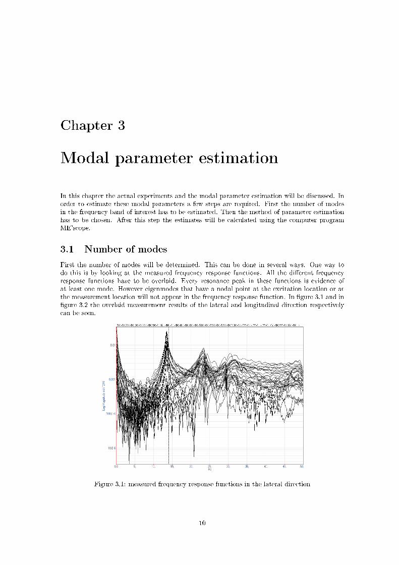
3.1 Number of modesFirst the number of modes will be determined. This can be done in several ways. One way todo this is by looking at the measured frequency response functions. All the di�erent frequencyresponse functions have to be overlaid. Every resonance peak in these functions is evidence ofat least one mode. However eigenmodes that have a nodal point at the excitation location or atthe measurement location will not appear in the frequency response function. In �gure 3.1 and in�gure 3.2 the overlaid measurement results of the lateral and longitudinal direction respectivelycan be seen.

Figure 3.1: measured frequency response functions in the lateral direction

10

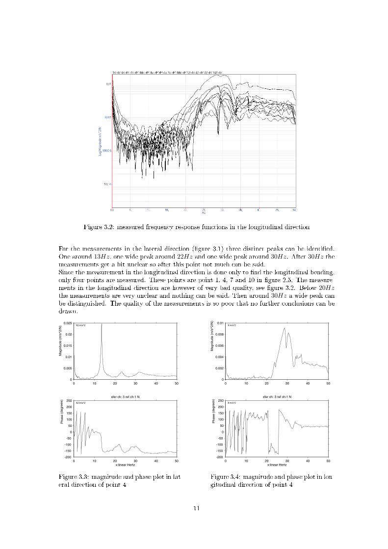
Figure 3.2: measured frequency response functions in the longitudinal direction

For the measurements in the lateral direction (�gure 3.1) three distinct peaks can be identi�ed.One around 13Hz, one wide peak around 22Hz and one wide peak around 30Hz. After 30Hz themeasurements get a bit unclear so after this point not much can be said.Since the measurement in the longitudinal direction is done only to �nd the longitudinal bending,only four points are measured. These points are point 1, 4, 7 and 10 in �gure 2.5. The measure-ments in the longitudinal direction are however of very bad quality, see �gure 3.2. Below 20Hzthe measurements are very unclear and nothing can be said. Then around 30Hz a wide peak canbe distinguished. The quality of the measurements is so poor that no further conclusions can bedrawn.

Magnitude (

m/s

^2/N

)P

hase (

degre

es)

Figure 3.3: magnitude and phase plot in lat-eral direction of point 4

Magnitude (

m/s

^2/N

)P

ha

se

(de

gre

es)

Figure 3.4: magnitude and phase plot in lon-gitudinal direction of point 4

11

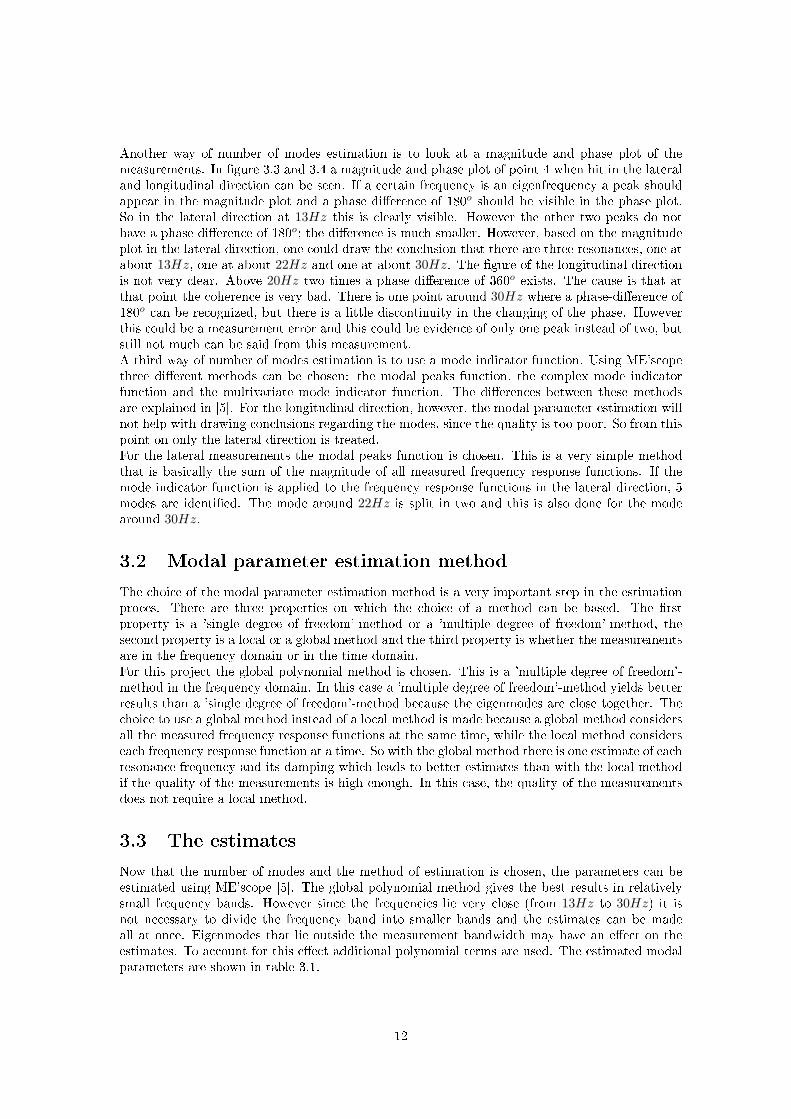
Another way of number of modes estimation is to look at a magnitude and phase plot of themeasurements. In �gure 3.3 and 3.4 a magnitude and phase plot of point 4 when hit in the lateraland longitudinal direction can be seen. If a certain frequency is an eigenfrequency a peak shouldappear in the magnitude plot and a phase di�erence of 180o should be visible in the phase plot.So in the lateral direction at 13Hz this is clearly visible. However the other two peaks do nothave a phase di�erence of 180o; the di�erence is much smaller. However, based on the magnitudeplot in the lateral direction, one could draw the conclusion that there are three resonances, one atabout 13Hz, one at about 22Hz and one at about 30Hz. The �gure of the longitudinal directionis not very clear. Above 20Hz two times a phase di�erence of 360o exists. The cause is that atthat point the coherence is very bad. There is one point around 30Hz where a phase-di�erence of180o can be recognized, but there is a little discontinuity in the changing of the phase. Howeverthis could be a measurement error and this could be evidence of only one peak instead of two, butstill not much can be said from this measurement.A third way of number of modes estimation is to use a mode indicator function. Using ME'scopethree di�erent methods can be chosen: the modal peaks function, the complex mode indicatorfunction and the multivariate mode indicator function. The di�erences between these methodsare explained in [5]. For the longitudinal direction, however, the modal parameter estimation willnot help with drawing conclusions regarding the modes, since the quality is too poor. So from thispoint on only the lateral direction is treated.For the lateral measurements the modal peaks function is chosen. This is a very simple methodthat is basically the sum of the magnitude of all measured frequency response functions. If themode indicator function is applied to the frequency response functions in the lateral direction, 5modes are identi�ed. The mode around 22Hz is split in two and this is also done for the modearound 30Hz.

3.2 Modal parameter estimation methodThe choice of the modal parameter estimation method is a very important step in the estimationproces. There are three properties on which the choice of a method can be based. The �rstproperty is a 'single degree of freedom'-method or a 'multiple degree of freedom'-method, thesecond property is a local or a global method and the third property is whether the measurementsare in the frequency domain or in the time domain.For this project the global polynomial method is chosen. This is a 'multiple degree of freedom'-method in the frequency domain. In this case a 'multiple degree of freedom'-method yields betterresults than a 'single degree of freedom'-method because the eigenmodes are close together. Thechoice to use a global method instead of a local method is made because a global method considersall the measured frequency response functions at the same time, while the local method considerseach frequency response function at a time. So with the global method there is one estimate of eachresonance frequency and its damping which leads to better estimates than with the local methodif the quality of the measurements is high enough. In this case, the quality of the measurementsdoes not require a local method.

3.3 The estimatesNow that the number of modes and the method of estimation is chosen, the parameters can beestimated using ME'scope [5]. The global polynomial method gives the best results in relativelysmall frequency bands. However since the frequencies lie very close (from 13Hz to 30Hz) it isnot necessary to divide the frequency band into smaller bands and the estimates can be madeall at once. Eigenmodes that lie outside the measurement bandwidth may have an e�ect on theestimates. To account for this e�ect additional polynomial terms are used. The estimated modalparameters are shown in table 3.1.

12

Mode Frequency [Hz] Damping [%]1 13.5 1.452 21.8 3.243 23.4 1.434 29.2 0.9995 30.4 1.96

Table 3.1: eigenfrequencies and damping ratios in the lateral direction

Now that the estimated modal parameters are known, their corresponding mode shapes can bedisplayed. The mode shapes are presented and evaluated in the next chapter.

13

Chapter 4

Evaluation

In this chapter the estimated modal parameters and their corresponding mode shapes are pre-sented, analysed and evaluated.

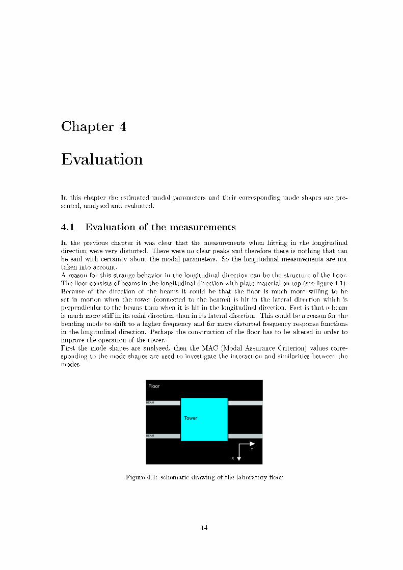
4.1 Evaluation of the measurementsIn the previous chapter it was clear that the measurements when hitting in the longitudinaldirection were very distorted. There were no clear peaks and therefore there is nothing that canbe said with certainty about the modal parameters. So the longitudinal measurements are nottaken into account.A reason for this strange behavior in the longitudinal direction can be the structure of the �oor.The �oor consists of beams in the longitudinal direction with plate material on top (see �gure 4.1).Because of the direction of the beams it could be that the �oor is much more willing to beset in motion when the tower (connected to the beams) is hit in the lateral direction which isperpendicular to the beams than when it is hit in the longitudinal direction. Fact is that a beamis much more sti� in its axial direction than in its lateral direction. This could be a reason for thebending mode to shift to a higher frequency and for more distorted frequency response functionsin the longitudinal direction. Perhaps the construction of the �oor has to be altered in order toimprove the operation of the tower.First the mode shapes are analysed, then the MAC (Modal Assurance Criterion) values corre-sponding to the mode shapes are used to investigate the interaction and similarities between themodes.

Tower

BEAM

BEAM

Floor

X

Y

Figure 4.1: schematic drawing of the laboratory �oor

14

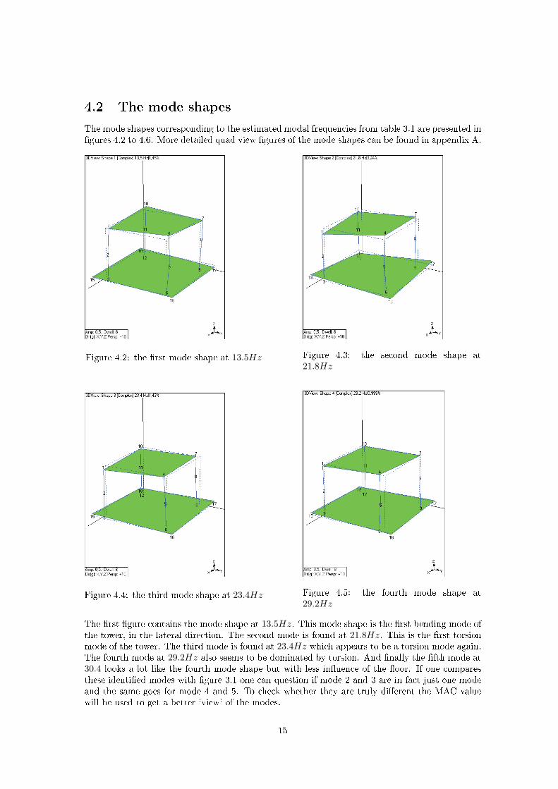
4.2 The mode shapesThe mode shapes corresponding to the estimated modal frequencies from table 3.1 are presented in�gures 4.2 to 4.6. More detailed quad view �gures of the mode shapes can be found in appendix A.

Figure 4.2: the �rst mode shape at 13.5Hz Figure 4.3: the second mode shape at21.8Hz

Figure 4.4: the third mode shape at 23.4Hz Figure 4.5: the fourth mode shape at29.2Hz

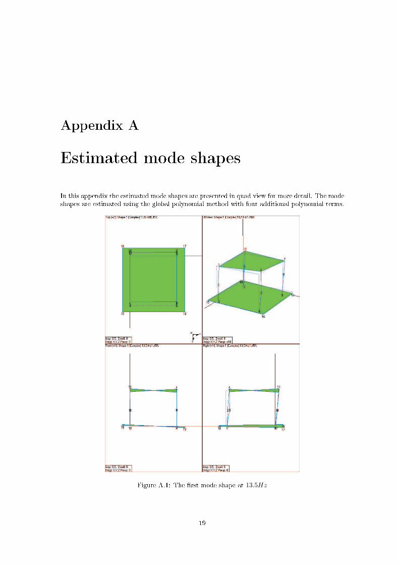
The �rst �gure contains the mode shape at 13.5Hz. This mode shape is the �rst bending mode ofthe tower, in the lateral direction. The second mode is found at 21.8Hz. This is the �rst torsionmode of the tower. The third mode is found at 23.4Hz which appears to be a torsion mode again.The fourth mode at 29.2Hz also seems to be dominated by torsion. And �nally the �fth mode at30.4 looks a lot like the fourth mode shape but with less in�uence of the �oor. If one comparesthese identi�ed modes with �gure 3.1 one can question if mode 2 and 3 are in fact just one modeand the same goes for mode 4 and 5. To check whether they are truly di�erent the MAC valuewill be used to get a better 'view' of the modes.

15

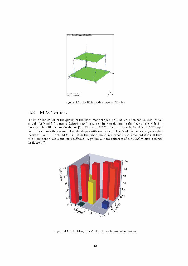
Figure 4.6: the �fth mode shape at 30.4Hz

4.3 MAC valuesTo get an indication of the quality of the �tted mode shapes the MAC criterion can be used. MACstands for Modal Assurance Criterion and is a technique to determine the degree of correlationbetween the di�erent mode shapes [1]. The auto MAC value can be calculated with ME'scopeand it compares the estimated mode shapes with each other. The MAC value is always a valuebetween 0 and 1. If the MAC is 1 than the mode shapes are exactly the same and if it is 0 thenthe mode shapes are completely di�erent. A graphical representation of the MAC values is shownin �gure 4.7.

4 1

2

3

4

5

1

32

5

Figure 4.7: The MAC matrix for the estimated eigenmodes

16

In the �gure it can be seen that all the values on the diagonal of the MAC matrix are equal toone. This is expected because on the diagonal every mode shape is compared with itself.Figure 4.7 shows that there is a fairly large correlation between mode 2 and 3 and between mode4 and 5. This means that they are related to each other. The value between 2 and 3 is 0.630 andthe value between 4 and 5 is 0.909. As stated before mode shape 4 and 5 are very similar. In�gure 3.1 it was di�cult to see two peaks so since these two have such a high MAC value thesemodes are just one mode. The reason that ME'scope recognized them as two di�erent modes isprobably a change in the circumstances during the measuring. In �gure 3.3 the peaks for mode 2and 3 also look like just one peak. However the MAC value of 0.630 is not high enough to drawthe conclusion that this also is only one mode although �gure 3.3 would suggest that. For thisconclusion some more research should be done.

4.4 DiscussionLooking at �gure 3.1 and �gure 3.3 the feeling arises that there are three modes present, althoughthe MAC values contradict this. However, it could very well be that during the measurements themeasurement environment was changed in such a way that the frequency at 22Hz shifted a little.So in spite of what the MAC value implies, the two modes at about 22Hz will be treated as onemode.The �rst mode is clearly the lateral bending and the other two, around 22Hz and 30Hz, aretorsion modes. The fact that there are two torsion modes instead of only one is not what wasexpected. It is possible that one of the two is the result of a resonance in the �oor. Also the widepeak in the longitudinal direction around 30Hz suggests that this is the real �rst torsion modeand the peak in the lateral direction around 22Hz is caused by the �oor.As mentioned earlier the �oor in the AES laboratory plays an important role in the measurements.Had the �oor been in�nitely sti�, then it was expected that the �rst mode that would appear, wouldbe the torsion mode. However the �rst mode that appears is the lateral bending around 14Hz. Itis very realistic to think that this is because of the construction of the �oor. As mentioned beforethe beams are much more willing to be set in motion in the lateral direction. Therefore the pointwhere the lateral bending appears could be shifted to a lower frequency. This phenomenon doesnot occur in the longitudinal direction because this is the axial direction of the beams and theyare much more sti� in this direction. This is probably the reason that no longitudinal bending canbe found in this frequency range. The longitudinal bending can probably be found at a frequencyhigher than the 50Hz-bandwidth. If the �oor was made more sti� in the lateral direction probablythe lateral bending would not occur at about 14Hz and the �rst mode would be the torsion modeas was expected.

17

Chapter 5

Conclusions and recommendations

In this report an experimental modal analysis of the tyre measuring tower is performed. As canbe seen in chapter 3 and 4 the three modal frequencies are found at about 13.5Hz, 22Hz and30Hz. So the actuator would have to be able to actuate up to about 10Hz.However, as it now seems, the �oor has a considerable e�ect on the measurements. If the �ooris altered to be sti�er in the lateral direction, the lateral bending mode will occur at a higherfrequency and the available bandwidth for vertical excitation increases. This larger bandwidth isdesired, because in research on the dynamic tyre behavior the bandwidth is desired to be as large aspossible. Since almost all vehicles have an eigenfrequency at about 15Hz (the wheel-hop mode), itis very interesting to increase the bandwidth so that actuation up to about 15Hz is possible. Thisalso implies that the actuator will be more expensive because the higher the actuation frequency,the higher the accelerations and velocities, the higher the price of the actuator.Although there is now a good idea of where the lowest eigenmodes appear, there still is room forimprovement of the accuracy. For further research it is important that the dynamic behavior of the�oor is known. If this behavior is known perhaps a measurement when hitting in the longitudinaldirection can also be done correctly. Furthermore not every point is measured in every directionso in order to get more accurate results this is also a point that can be considered.Finally, in this experiment the mass of the actuator has been compensated for. However if areal actuator is mounted on the measuring tower, it can also in�uence the behavior of the tower,because the wheel cannot move up and down without any resistance. Furthermore, the mass of thereal actuator can be di�erent than the dummy mass mounted on the tower during the experiments.This can also in�uence the measurements.

18

Appendix A

Estimated mode shapes

In this appendix the estimated mode shapes are presented in quad view for more detail. The modeshapes are estimated using the global polynomial method with four additional polynomial terms.

Figure A.1: The �rst mode shape at 13.5Hz

19

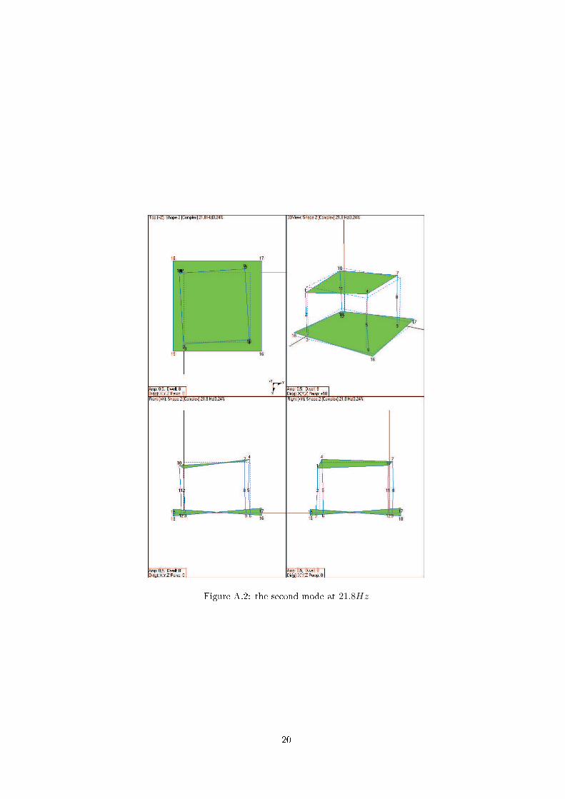
Figure A.2: the second mode at 21.8Hz

20

Figure A.3: the third mode at 23.4Hz

21

Figure A.4: the fourth mode at 29.2Hz

22

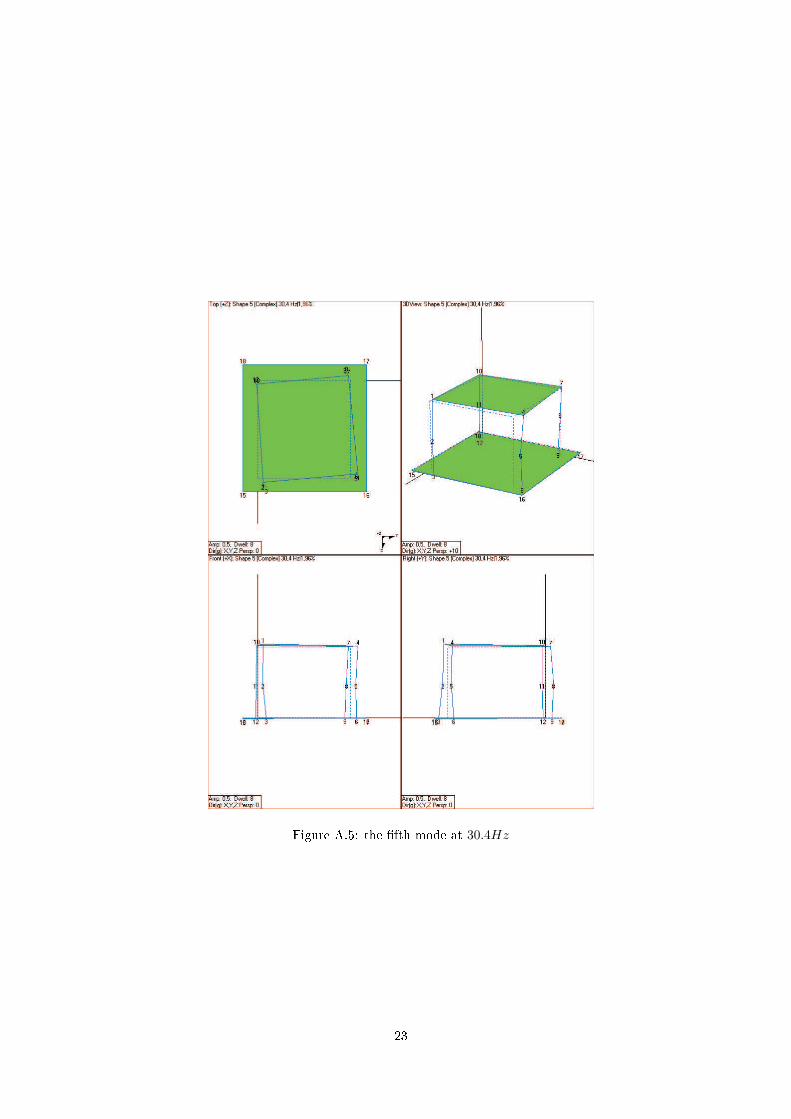
Figure A.5: the �fth mode at 30.4Hz

23

Bibliography

[1] B. de Kraker: A Numerical-Experimental Approach in Structural Dynamics, 2000. Lecturenotes nr. 4748

[2] J.J. Kok and M.J.G. van de Molengraft: Signaalanalyse, 2003. Lecture notes course nr. 4A250

[3] R.J.E. Merry: Experimental Modal Analysis of the H-drive. Report No. DCT 2003.78

[4] M.L.J. Verhees: Experimental Modal Analysis of a Turbine Blade. Report No. DCT 2004.120

[5] Vibrant technology Inc.: ME'ScopeVES operating manual, 2003

[6] DSP technology Inc.: Siglab User Guide, 1998

24