Experimental realization of post-selected weak measurements on an NMR

quantum processor

Dawei Lu,1 Aharon Brodutch,1, ∗ Jun Li,1, 2 Hang Li,1, 3 and Raymond Laflamme1, 4, †

1Institute for Quantum Computing and Department of Physics & Astronomy,

University of Waterloo, Waterloo, Ontario N2L 3G1, Canada

2Department of Modern Physics, University of Science

and Technology of China, Hefei, Anhui 230026, China

3Department of Physics, Tsinghua University, Beijing 100084, China

4Perimeter Institute for Theoretical Physics, Waterloo, Ontario N2L 2Y5, Canada

(Dated: April 27, 2018)

The ability to post-select the outcomes of an experiment is a useful theoretical concept and

experimental tool. In the context of weak measurements, post-selection can lead to surprising

results such as complex weak values outside the range of eigenvalues. Usually post-selection

is realized by a projective measurement, which is hard to implement in ensemble systems such

as NMR. We demonstrate the first experiment of a weak measurement with post-selection

on an NMR quantum information processor. Our setup is used for measuring complex weak

values and weak values outside the range of eigenvalues. The scheme for overcoming the

problem of post-selection in an ensemble quantum computer is general and can be applied to

any circuit-based implementation. This experiment paves the way for studying and exploiting

post-selection and weak measurements in systems where projective measurements are hard

to realize experimentally.

PACS numbers:

I. INTRODUCTION

Many fundamental experiments in quantum mechanics can be written and fully understood in

terms of a quantum circuit [1]. The current state of the art, however, provides a poor platform for

implanting these circuits on what can be considered a universal quantum computer. The limited

number of independent degrees of freedom that can be manipulated efficiently limit the possible

experiments. Many popular experiments involving a small number of qubits include some type of

∗Electronic address: aharon.brodutch@uwaterloo.ca†Electronic address: laflamme@iqc.ca

arX

iv:1

311.

5890

v2 [

quan

t-ph

] 6

Jun

201

4

2

post-selection. By post-selecting, experimenters condition their statistics only on those experiments

that (will) meet a certain criteria such as the result of a projective measurement performed at the

end of the experiment. Such conditioning produces a number of surprising effects like strange

weak values [2] and nonlinear quantum gates [3]. Although they are sometimes described via

quantum circuits, experiments involving post-selection are usually implemented in a dedicated

setup which is not intended to act as a universal quantum processor. For example in current

optical implementations [4, 5] the addition of more gates would require extra hardware.

Nowadays, implementations of quantum computing tasks in NMR architectures provide a good

test-bed for up to 12 qubits [6]. Universal quantum circuits can be implemented on mid-scale

(5-7 qubit) NMR quantum computers with the development of high-fidelity control [7]. However,

the difficulty in performing projective measurements poses a handicap with the implementation of

circuits involving post-selection. Here we will show how to overcome this difficulty theoretically

and experimentally, in the setting of weak measurements.

Weak measurements provide an elegant way to learn something about a quantum system S in

the interval between preparation and post-selection [8]. When the interaction between S and a

measuring device M is weak enough, the back-action is negligible [9]. Moreover the effective evo-

lution of the measuring device during the measurement is proportional to a weak value, a complex

number which is a function of the pre-selection, post-selection and the desired observable. These

weak values allow us to make statements that would otherwise be in the realm of counterfactuals

[10, 11]. Weak values have been interpreted as complex probabilities [12] and/or element of reality

[13] and, although somewhat controversial [14–16], they are used to describe a number of funda-

mental issues in quantum mechanics including: Non-locality in the two slit experiment [9], the

trajectories of photons [17], the reality of the wave function[18], Hardy’s paradox[10, 11, 19], the

three box paradox [8, 13, 20], measurement precision-disturbance relations [5, 21] and the Leggett-

Garg inequality [22–24]. Recently the amplification effect associated with large real and imaginary

weak values was used in practical schemes for precision measurements. While these schemes cannot

overcome the limits imposed by quantum mechanics, they can be used to improve precision under

various types of operational imitations such as technical noise [25].

Experimental realizations of weak measurements have so far been limited to optics with only a

few recent exceptions [24, 26]. In all cases post-selection was done using projective measurements

that physically select events with successful post-selection. Optical experiments (e.g ref. [27])

exploit the fact that one degree of freedom can be used as the system while another (usually a

continuous degree of freedom) can be used as the measuring device. Post-selection is achieved

3

by filtering out photons that fail post-selection and the readout is done at the end only on the

surviving systems. This type of filtering is outside the scope of ensemble quantum computers

where all operations apart from the final ensemble measurement are unitary. One can overcome

the difficulty by either including a physical filter or by finding some way for post-selection using

unitary operations. The former poses a technical challenge as well as a conceptual deviation from

the circuit model. In what follows we show how to perform the latter by resetting the measuring

device each time post-selection fails. Our theoretical proposal is compatible with a number of

current implementation of quantum processors such as such as liquid and solid state NMR[6, 28–

30], electron spin qubits [31, 32] and rare earth crystal implementations [33].

We begin by describing the weak measurement process for qubits and the theoretical circuit for

weak measurements on an ensemble quantum computer (Fig. 1). Next we describe our experiment

in detail (Fig. 2). We demonstrate two properties of weak values associated with post-selection:

weak values outside the range of eigenvalues and imaginary weak values (Figs. 3, 4). We conclude

with a discussion of future applications

II. WEAK MEASUREMENTS

The weak measurement procedure (for qubits) [34] involves a system S qubit initially prepared in

the state |ψ〉S and a measuring device qubit initially in the state |Mi〉M such that 〈Mi|σz |Mi〉 = 0.

The system and measuring device are coupled for a very short time via the interaction Hamiltonian

Hi = δ(t− ti)gσSnσMz with the coupling constant g << 1 and σn = n · ~σ a Pauli observable in the

direction n. This is followed by a projective (post-selection) measurement on S with outcome |φ〉S .

Up to normalization we have

|ψ,Mi〉S,M → e−igσSnσMz |ψ,Mi〉S,M

→ cos(g)〈φ|ψ〉 |φ,Mi〉S,M − i sin(g) 〈φ|σn |ψ〉σMz |φ,Mi〉S,M (1)

The unnormalized state of M at the end is

|Mf 〉 = 〈φ|ψ〉[cos(g)11M − i sin(g){σn}wσMz ] |Mi〉S,M (2)

where

{σn}w =〈φ|σSn |ψ〉〈φ|ψ〉

(3)

4

is the weak value of σn. We can now take the weak measurement approximation |g{σn}w| << 1

so that up to first order in g we have

|Mf 〉 ≈ e−ig{σn}wσMz |Mi〉 (4)

The measurement device is rotated by g{σn}w around the z-axis. Note that this is the actual

unitary evolution (at this approximation), not an average unitary. If we set the measuring device

to be in the initial state 1√2[|0〉+ |1〉], the expectation value for σMm = m · ~σM will be

〈Mf |σMm |Mf 〉 ≈ 〈Mi| (11 + ig{σn}∗wσMz )σMm (11− ig{σn}wσMz ) |Mi〉 (5)

≈ 〈Mi|σMm |Mi〉+ ig 〈Mi| {σn}∗wσMz σMm − {σn}wσMm σMz |Mi〉 (6)

= 〈Mi|σMm |Mi〉+ igRe({σn}w) 〈Mi|σMz σMm − σMm σMz |Mi〉

+ gIm({σn}w) 〈Mi|σMz σMm + σMm σMz |Mi〉 (7)

Choosing m appropriately we can get the real or imaginary part of the weak value.

The scheme above is based on the fact that S was post-selected in the correct state |φ〉. Since

this cannot be guaranteed in an experiment, we need to somehow disregard those events where

post-selection fails. As noted previously, the standard method for implementing the post-selection

is by filtering out the composite S,M systems that fail post-selection. While this is relatively

simple in some implementations it is not a generic property of a quantum processor. In particular

post-selection is not implicit in the circuit model. The method to overcome this problem is to reset

the measuring device whenever post-selection fails.

One way to implement the controlled reset (see Fig. 1) is by using a controlled depolarizing

gate with the following properties

|φ〉 〈φ|S ⊗ ρM → |φ〉 〈φ|S ⊗ ρM

|φ⊥〉 〈φ⊥|S ⊗ ρM → |φ⊥〉 〈φ⊥|S ⊗ 11/2, (8)

where ρM is an arbitrary state and |φ⊥〉S is the orthogonal state to the post-selection 〈φ⊥|φ〉 = 0.

This gate is not unitary and requires an ancillary system A. It can be constructed by setting

ρA = 11/2 and using a controlled-SWAP with the swap between A and M. To keep the control

in the computational basis, we preceded the controlled-SWAP gate by US†φ where Uφ |0〉 = |φ〉.

At the readout stage we need to measure the observable |0〉 〈0| which will give the probability

of post-selection p0 as well as 〈σMm 〉. Finally we divide 〈σMm 〉 by p0 to obtain the weak value.

If we are only interested in reading out the real or imaginary part of the weak value we can

5

further simplify this operation by a controlled dephasing in a complementary basis to σMm . This

allows us to replace the controlled-SWAP by a controlled-controlled-phase with M as the target

and A,S as the control (see Fig. 2b). In our experimental setup we used the latter (simplified)

approach. A controlled-controlled-σz was used in the post-selection for measuring real weak values

and controlled-controlled-σx was used for complex weak values.

Depolarizing

Pre-selection Post-selection ReadoutWeak measurement

WeakMeasurement

|Ψ >

ρi

<σ z>

<σ n>

System

Measuring device

U Φ†

FIG. 1: (color online). Conceptual circuit for post-selected weak measurements. The system S is prepared

in the state |ψ〉, it then interacts weakly with the measurement device M (the weak measurement stage).

Post-selection is performed by a controlled depolarizing channel in the desired basis, Eq (8), decomposed

into a rotation U†φ followed by a contolled depolarizing in the computational basis. Finally at the readout

stage we get the probability of post-selection p0 from 〈σSz 〉 = 2p0−1. The exception values 〈σM

n 〉 are shifted

by a factor proportional to the weak value and decayed by a factor p0.

III. EXPERIMENTAL IMPLEMENTATION

We conducted three types of experiments. In each experiment we prepared S in an initial state

on the x−z plane, cos(θ) |0〉S+sin(θ) |1〉S , the weak measurement observable was a Pauli operator

in the x−y plane, cos(α)σSx +sin(α)σSy and the post-selection was always the |0〉S state. In the first

experiment (Fig. 3b) we set α = 0 to make a measurement of σx and varied the coupling strength

from g = 0.05 to g = 0.7. We used three different initial states: θ = π/4 - corresponding to a

measurement where the weak value coincides with the result of a projective (g = π/4) measurement,

θ = 1.2 - where we were able to observe a large weak value,{σx}w = 2.57, at g = 0.05 , and θ = 1.4

- where the weak value (first order) approximation is off by more than 10% at g = 0.05. Next we

6

kept the coupling constant at g = 0.1 and varied over θ to observe real weak values both inside

and outside the range of eigenvalues [−1, 1] (Fig. 4a). Finally we measured complex weak values

with an absolute magnitude of 1 by keeping the initial state constant, θ = π/4, and varying over

the measurement direction α at g = 0.1 (Fig. 4b).

All experiments were conducted on a Bruker DRX 700MHZ spectrometer at room temperature.

Our 3-qubit sample was 13C labeled trichloroethylene (TCE) dissolved in d-chloroform. The struc-

ture of the molecule is shown in Fig. 2a, where we denote C1 as qubit 1, C2 as qubit 2, and H as

qubit 3. The internal Hamiltonian of this system can be described as

H =3∑j=1

πνjσjz +

π

2(J13σ

1zσ

3z + J23σ

2zσ

3z)

+π

2J12(σ

1xσ

2x + σ1yσ

2y + σ1zσ

2z), (9)

where νj is the chemical shift of the jth spin and Jij is the scalar coupling strength between spins i

and j. As the difference in frequencies between C1 and C2 is not large enough to adopt the (NMR

[41]) weak J-coupling approximation [35], these two carbon spins are treated in the strongly coupled

regime. The parameters of the Hamiltonian are obtained by iteratively fitting the calculated and

observed spectra through perturbation, and shown in the table of Fig. 2a.

We label C1 as the ancilla A, C2 as the measuring deviceM, and H as the system S (Fig. 2b).

Each experiment can be divided into four parts: (A) Pre-selection: Initializing the ancilla to the

identity matrix 11/2, the measurement device to 1/√

2(|0〉+|1〉), and the system to cosθ|0〉+sinθ|1〉.

(B) Weak measurement: Interaction between the measuring device and system, denoted by Uw in

the network. (C) Post-selection of the system in the state |0〉. (D) Measurement: 〈σMy 〉 on the

measuring device (〈σMz 〉 for the imaginary part) and 〈σSz 〉 on the system. The experimental details

of the four parts above are as follows.

(A) Pre-selection: Starting from the thermal equilibrium state, first we excite the ancilla C1 to

the transverse field by a π/2 rotation, followed with a gradient pulse to destroy coherence leaving

C1 in the maximally mixed state 11/2. Next we create the pseudopure state (PPS) of C2 (M) and

H (S) with deviation 11⊗|00〉 〈00| using the spatial average technique [30]. For traceless observables

and unital evolution the identity part of the PPS can be treated as noise on top of a pure state.

The spectra of the PPS followed by π/2 readout pulses are shown in the upper part of Fig. 3a.

The readout pulses are applied on C2 (left figure) and H (right figure), respectively. Two peaks are

generated in the PPS spectra because C1 is in the maximally mixed state 11/2, and these two peaks

are utilized as the benchmark for the following experiments. Finally we apply one Hadamard gate

7

4

C1 C2 H T1(s) T2(s)

C1 21784.6 13.0 0.3 0.45 0.02

C2 103.03 20528.0 8.9 0.3 1.18 0.02

H 8.52 201.45 4546.9 8.9 0.3 1.7 0.2

H|0⟩

I

UW

R(θ)

ZM1

M2

HR(θ)

UW

Hadamardexp(-i θ σy)

exp(-i g σx σz)

Z exp(-i π/2 σz)M1 σy

σzM2

C1:

C2:

H: |0⟩

(a)

(b) C1-Ancilla; C2-Measuring Device; H-System.

C2 C1

H

Cl Cl

Cl

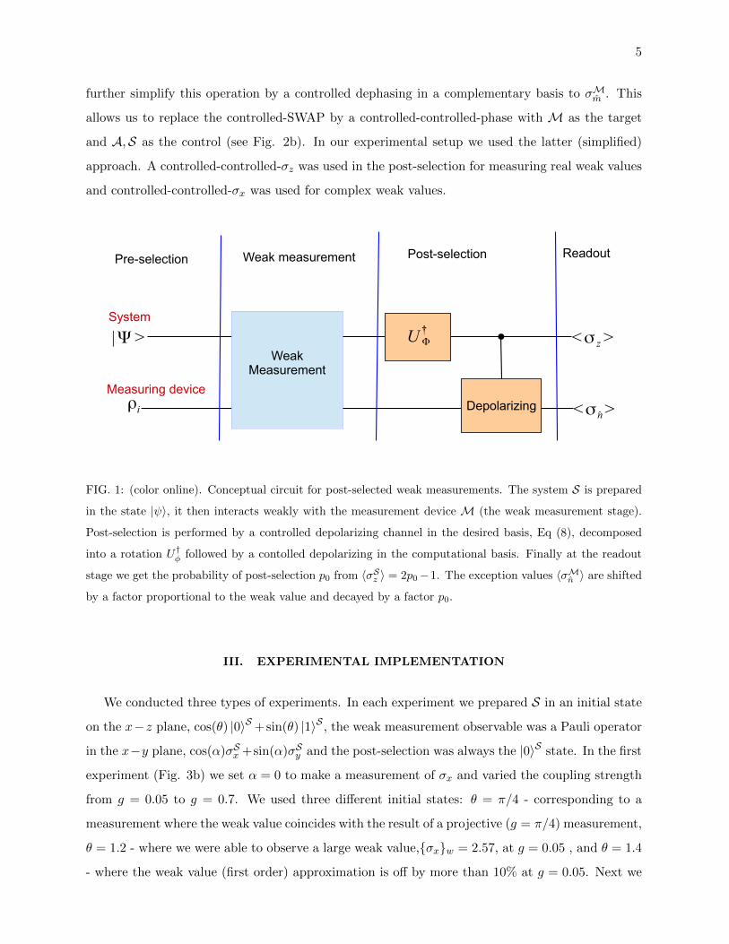
FIG. 2: (color online). (a) Experimental implementation of a weak measurement in NMR using trichloroethy-

lene in which the two 13C and one 1H spins form a 3-qubit sample. In the parameter table the diagonal

elements are the chemical shifts (Hz), and the off-diagonal elements are scalar coupling strengths (Hz). T1

and T2 are the relaxation and dephasing time scales. (b) The quantum network used to realize the post-

selected weak measurement in the experiment with C1 as the ancilla A, C2 as the measuring deviceM, and

H as the system S. Post-selection of |0〉S was achieved using the controlled-controlled-Z gate so that M

is dephased when post-selection fails. The final measurements give the expectation values 〈σSz 〉 and 〈σM

y 〉

which are used to calculate the weak value via Eq (13).

on C2 and one Ry(θ) = e−iθσy rotation on H. At the end of this procedure the state is

ρini = 11⊗ 1

2(|0〉+ |1〉)(〈0|+ 〈1|)⊗ (cosθ|0〉+ sinθ|1〉)(cosθ〈0|+ sinθ〈1|). (10)

(B) Weak measurement: The unitary operator to realize the weak measurement

Uw = e−igσ2nσ

3z . (11)

can be simulated by the interaction term σ2zσ3z between C2 and H using the average Hamiltonian

theory [36]. However, since the internal Hamiltonian contains a strongly coupling term and the

refocusing scheme requires the WAHUHA-4 sequence [37] we adopted the gradient ascent pulse

engineering (GRAPE) technique [38, 39] to improve the fidelity (see discussion below).

(C) Post-selection: In order to mimic the post-selection of |0〉 on the system spin H in NMR,

we introduce an ancilla qubit C1 in the maximally mixed state 11. The controlled resetting noise

operation is a controlled-controlled-σz gate

11⊗ 11⊗ 11− |1〉〈1| ⊗ |1〉〈1| ⊗ 11 + |1〉〈1| ⊗ |1〉〈1| ⊗ σz. (12)

8

If post-selection is successful, the measurement device will point to the weak value. Otherwise

the measurement device will become dephased and the expectation value⟨σ2y⟩

will be reset to 0.

For the measurement of complex weak values we used a standard Toffoli and applied the same

reasoning.

(D) Measurement: Finally we measure the expectation value 〈σ2y〉 on C2 and 〈σ3z〉 on H, to

calculate the weak value by the expression

Re({σx}w) ≈〈σ2y〉

g(〈σ3z〉+ 1). (13)

For the imaginary part we similarly use⟨σ2z⟩.

Since the timescales for the experiment are much shorter than T1 the evolution is very close to

unital.

In the experiment, the π/2 rotation of H is realized by the hard pulse with a duration of 10 µs.

All the other operations are implemented through GRAPE pulses to achieve high-fidelity control.

These GRAPE pulses are designed to be robust to the inhomogeneity of the magnetic field, and

the imprecisions of the parameters in the Hamiltonian. For the two selective π/2 excitations on C1

and C2, the GRAPE pulses are generated with the length 1.5 ms, segments 300 and fidelity over

99.95%. These two pulses are only used for the preparation and observation of PPS. Besides these

two GRAPE pulses, the PPS preparation involves another GRAPE pulse of 10 ms and 99.99%

fidelity for the creation of two-body coherence. The top spectra in Fig. 3a are the PPS both on

C2 and H, which are used as the benchmark for the following experiments.

The main body of the network shown in Fig. 2b, including the pre-selection, weak measurement

and post-selection, is calculated by a single GRAPE pulse. Since we have to alter the initial state by

θ and interaction strength g in the experiment, we have used different GRAPE pulses to implement

the experiments with different group of parameters. All of these GRAPE pulses have the same

length: 20 ms, and fidelity over 99.98%.

There are two essential advantages in utilizing the GRAPE pulses: reducing the error accu-

mulated by the long pulse sequence if we directly decompose the network, and reducing the error

caused by decoherence. Because the Uw evolution is supposed to be very “weak”, the intensity of

the output signal is quite small. Moreover, the calculated weak values are more sensitive to the

intensity of the signal, because the small g in the denominator (Eq 13) will amplify the errors in

the experiment. Therefore, we need to achieve as accurate coherent control as we can to obtain

precise experimental results. The direct decomposition of the original network requires many single

rotations, as well as a relatively long evolution time. For example, an efficient way to decompose

9

the controlled-controlled-σz gate is by six CNOT gates and several one qubit gates [40], which

requires more than 50 ms in our experimental condition. Therefore, using short GRAPE pulses of

high fidelity we were able to decrease the potential errors due to decoherence and imperfect imple-

mentation of the long pulse sequence. Fig. 3a shows the experimental spectra compared with the

simulated one in the case g = 0.05 and θ = 1.4. The top plots are the reference (PPS) spectra while

the bottom are the spectra measured at the end of the experiment. The predicted value of 〈σ2y〉 in

this case is only 1.67%. However, since the experimental spectra are very close to the simulated

one, we can obtain a good result after extracting the data. The effects of decoherence in the case

of small post-selection probabilities values can be seen in Fig. 3b where the experimental values

are consistently lower than the theoretical predictions. Since decoherence reduces the expectation

values the results of Eq (13) will be more sensitive to decoherence as 〈σ3z〉 → −1.

In the first experiment we varied the interaction strength g = 0.05 to g = 0.7 for α = 0 and

three different initial states θ = 1.4, θ = 1.2, and θ = π/4. We obtained the weak value through

a final measurement of 〈σ2y〉 on the measuring device C2 and 〈σ3z〉 on the system H, respectively.

The weak value {σx}w was calculated through Eq (13), with the result shown in Fig. 3b. The

error bars were obtained by repeating the experiment four times. The large error bars in the weak

values at small values of g and low post-selection probabilities are a result of imperfect calibration

of the low experimental signals obtained at that range.

In the second experiment we studied the behavior of measured weak values as a function of the

initial state parameter θ at g = 0.1 and α = 0. The theoretical weak value should be tan(θ) (at

g → 0). We compared our results with a theoretical curve at g = 0.1 (Fig. 4a). As expected this

curve diverges from the weak value of tan(θ) as the overlap between the pre and post-selection

vanishes and second order terms become more dominant. The experimental data matches with the

smooth part of the curve. When θ is very close to π/2, we were unable to measure the extremely

low NMR signals due to the signal-to-noise ratio(SNR) issues, moreover decoherence effects become

more prominent at these values (see discussion above).

In the final experiment we measured both the real part and imaginary parts of the weak value

(Fig. 4b). We set θ = π/4 and g = 0.1, and changed α, the observable of the measuring device C2.

The expected weak values have an absolute magnitude of 1 and the overlap between the pre and

post-selected state is 1/√

2. To measure the imaginary part, we replaced the controlled-controlled-

σz gate in Fig. 2b with a controlled-controlled-σx gate, and measured the expectation value 〈σ2z〉

on the measuring device C2. The other parts of the experiments remain the same. In Fig. 2b

we can see the real part and imaginary part of the weak value along with the parameter α. The

10

(a)

(b)

0 0.1 0.2 0.3 0.4 0.5 0.6 0.7 0.80

1

2

3

4

5

6

g

wea

k va

lue

<σx>

Initial State cosθ|0>+sinθ|1>

θ = 1.4 (Theo)θ = 1.4 (Exp)θ = 1.2 (Theo)θ = 1.2 (Exp)θ = π/4 (Theo)θ = π/4 (Exp)

2.032.042.052.062.07x 10

4NMR Frequency (Hz)

NM

R sig

nal (

Arb.

Uni

t)

C2 Spectra

simulationexperiment

4400445045004550460046504700NMR Frequency (Hz)

NM

R sig

nal (

Arb.

Uni

t)

H Spectra

simulationexperiment

PPS PPS

g=0.05; θ=1.4g=0.05; θ=1.4

FIG. 3: (color online). (a) The spectra for each qubit (bottom spectrum) was compared with the reference

PPS (top spectrum) to obtain the expectation values 〈σMy 〉 on C2 and 〈σS

z 〉 on H. To observe the signal on H,

we applied π/2 readout pulses after the sequence. The spectra in the figure are for g = 0.05 and θ = 1.4, the

simulated spectra (blue) fit well with the experimental one (red). (b) Weak values for various initial states,

cos(θ) |0〉S +sin(θ) |1〉S , were calculated using Eq (13) and compared the theoretical predictions as a function

of the measurement strength from g = 0.05 to g = 0.7. The solid curves are theoretical predictions without

the weak measurement approximation. When the overlap between the pre and post-selection, cos(θ) is large

enough we get very close to the asymptotic g → 0 value at g ≥ 0.05. However for θ = 1.4 the interaction

was not weak enough at g = 0.05. The error bars are plotted by repeating each experiment four times. At

low post-selection probabilities we see observed values decrease due to decoherence.

11

0 0.5 1 1.5

0

0.2

0.4

0.6

0.8

1

1.2

α (g=0.1)

wea

k va

lue

<cosασ x-s

inασ y>

Initial State cos(π/4)|0>+sin(π/4)|1>

RealImag

0 0.5 1 1.5 2 2.5 3-5

0

5

θ (g=0.1)

wea

k va

lue

<σx>

Initial State cosθ|0>+sinθ|1>

simulationexperiment

(a) (b)

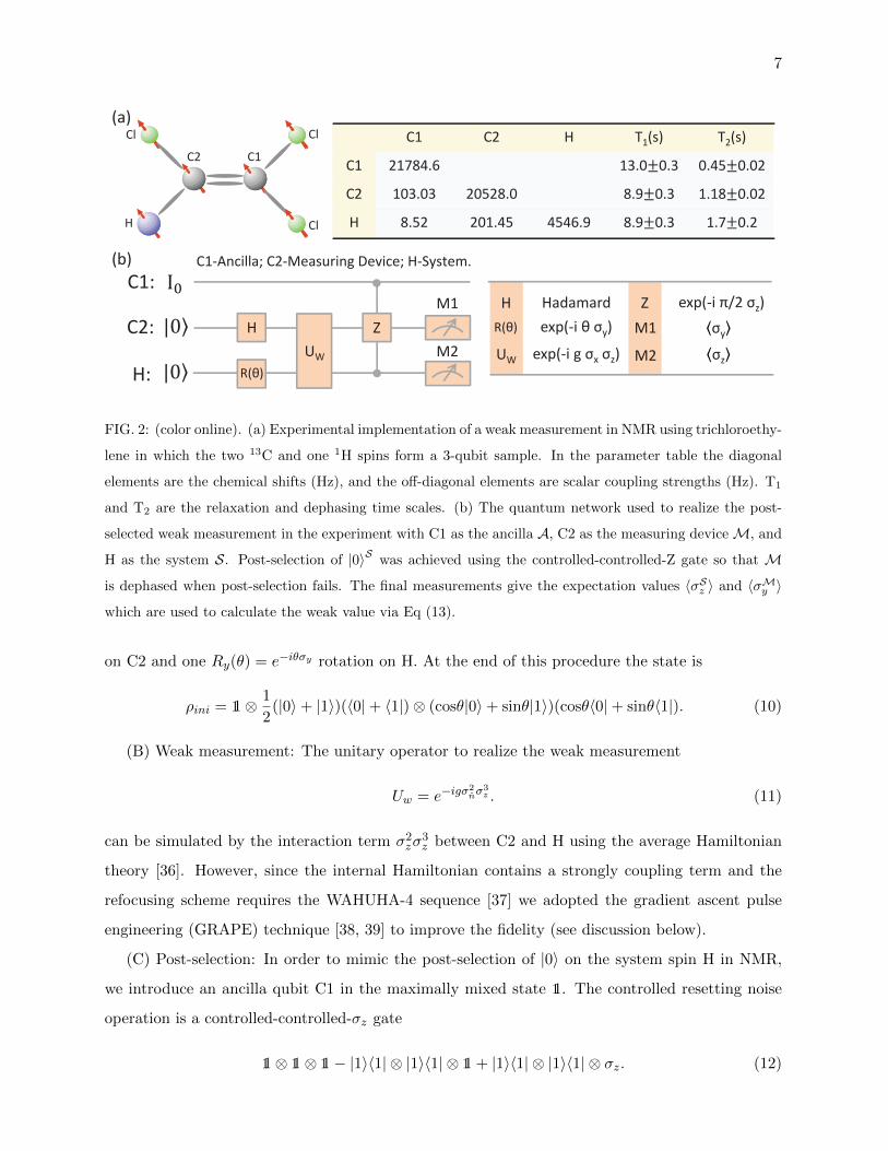
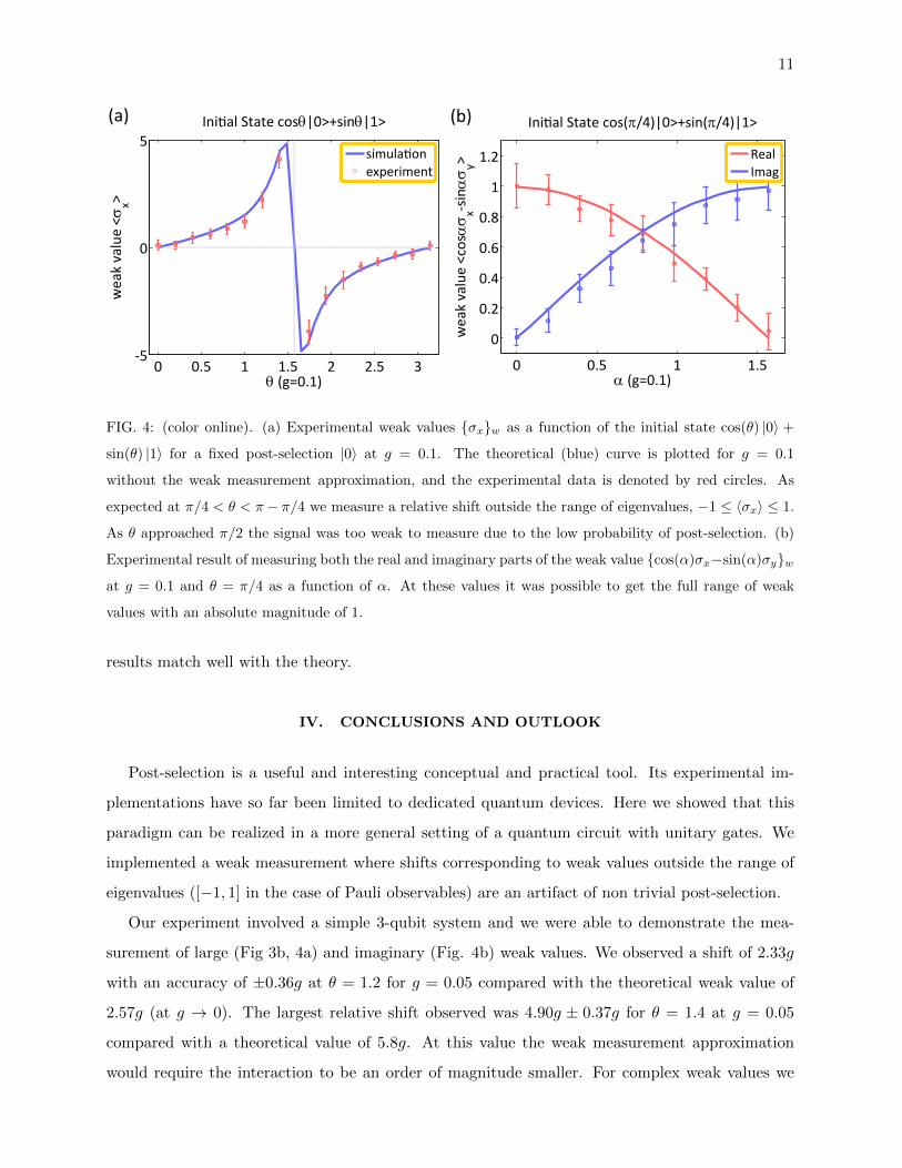
FIG. 4: (color online). (a) Experimental weak values {σx}w as a function of the initial state cos(θ) |0〉 +

sin(θ) |1〉 for a fixed post-selection |0〉 at g = 0.1. The theoretical (blue) curve is plotted for g = 0.1

without the weak measurement approximation, and the experimental data is denoted by red circles. As

expected at π/4 < θ < π − π/4 we measure a relative shift outside the range of eigenvalues, −1 ≤ 〈σx〉 ≤ 1.

As θ approached π/2 the signal was too weak to measure due to the low probability of post-selection. (b)

Experimental result of measuring both the real and imaginary parts of the weak value {cos(α)σx−sin(α)σy}wat g = 0.1 and θ = π/4 as a function of α. At these values it was possible to get the full range of weak

values with an absolute magnitude of 1.

results match well with the theory.

IV. CONCLUSIONS AND OUTLOOK

Post-selection is a useful and interesting conceptual and practical tool. Its experimental im-

plementations have so far been limited to dedicated quantum devices. Here we showed that this

paradigm can be realized in a more general setting of a quantum circuit with unitary gates. We

implemented a weak measurement where shifts corresponding to weak values outside the range of

eigenvalues ([−1, 1] in the case of Pauli observables) are an artifact of non trivial post-selection.

Our experiment involved a simple 3-qubit system and we were able to demonstrate the mea-

surement of large (Fig 3b, 4a) and imaginary (Fig. 4b) weak values. We observed a shift of 2.33g

with an accuracy of ±0.36g at θ = 1.2 for g = 0.05 compared with the theoretical weak value of

2.57g (at g → 0). The largest relative shift observed was 4.90g ± 0.37g for θ = 1.4 at g = 0.05

compared with a theoretical value of 5.8g. At this value the weak measurement approximation

would require the interaction to be an order of magnitude smaller. For complex weak values we

12

were able to demonstrate the full spectrum of complex weak values with unit absolute magnitude.

Our scheme has the advantage that it can be extended to systems with more qubits without

significant changes. Implementations on a four qubit system will allow the first fully quantum im-

plementation of the three box paradox and further extensions will allow more intricate experiments

such as the measurement of the wave-function and measurement-disturbance relations which have

so far been limited to optical implementations, often with classical light. The reasonably large

number of qubits that can be manipulated in NMR systems will also allow more intricate experi-

ments that are not possible in optics. It remains an open question whether our techniques can be

used for precision measurements in the same way as they are used in optics. Given that this is the

first implementation of weak measurements in NMR there is still much to be explored.

We thank Marco Piani and Sadegh Raeisi for comments and discussion. This work was sup-

ported by Industry Canada, NSERC and CIFAR. J. L. acknowledges National Nature Science

Foundation of China, the CAS, and the National Fundamental Research Program 2007CB925200.

[1] D. Deutsch, Proceedings of the Royal Society of London. A. Mathematical and Physical Sciences 400,

97 (1985), URL http://rspa.royalsocietypublishing.org/content/400/1818/97.short.

[2] Y. Aharonov, D. Z. Albert, and L. Vaidman, Physical Review Letters 60, 1351 (1988), URL http:

//prl.aps.org/abstract/PRL/v60/i14/p1351_1.

[3] S. Lloyd, L. Maccone, R. Garcia-Patron, V. Giovannetti, Y. Shikano, S. Pirandola, L. A. Rozema,

A. Darabi, Y. Soudagar, L. K. Shalm, et al., Physical Review Letters 106, 040403 (2011), URL http:

//prl.aps.org/abstract/PRL/v106/i4/e040403.

[4] J. S. Lundeen, Ph.D. thesis, University of Toronto (2006).

[5] L. A. Rozema, A. Darabi, D. H. Mahler, A. Hayat, Y. Soudagar, and A. M. Steinberg, Physical Review

Letters 109, 100404 (2012), URL http://prl.aps.org/abstract/PRL/v109/i10/e100404.

[6] C. Negrevergne, T. Mahesh, C. Ryan, M. Ditty, F. Cyr-Racine, W. Power, N. Boulant, T. Havel,

D. Cory, and R. Laflamme, Physical Review Letters 96, 170501 (2006), URL http://prl.aps.org/

abstract/PRL/v96/i17/e170501.

[7] I. S. Oliveira and R. M. Serra et. al, Philosophical Transactions of the Royal Society A 370, 4613

(2012).

[8] Y. Aharonov and L. Vaidman, Journal of Physics A: Mathematical and General 24, 2315 (1991), URL

http://iopscience.iop.org/0305-4470/24/10/018.

13

[9] J. Tollaksen, Y. Aharonov, A. Casher, T. Kaufherr, and S. Nussinov, New Journal of Physics 12,

013023 (2010), URL http://iopscience.iop.org/1367-2630/12/1/013023.

[10] Y. Aharonov, A. Botero, S. Popescu, B. Reznik, and J. Tollaksen, Physics Letters A 301, 130 (2002),

URL http://www.sciencedirect.com/science/article/pii/S0375960102009866.

[11] K. Mølmer, Physics Letters A 292, 151 (2001), URL http://www.sciencedirect.com/science/

article/pii/S0375960101007836.

[12] H. F. Hofmann, arXiv preprint arXiv:1303.0078 (2013).

[13] L. Vaidman, Foundations of Physics 26, 895 (1996), URL http://link.springer.com/article/10.

1007/BF02148832.

[14] A. Peres, Physical Review Letters 62, 2326 (1989).

[15] Y. Aharonov and L. Vaidman, Physical Review Letters 62, 2327 (1989).

[16] A. Leggett, Physical Review Letters 62, 2325 (1989).

[17] S. Kocsis, B. Braverman, S. Ravets, M. J. Stevens, R. P. Mirin, L. K. Shalm, and A. M. Steinberg,

Science 332, 1170 (2011), URL http://www.sciencemag.org/content/332/6034/1170.short.

[18] J. S. Lundeen, B. Sutherland, A. Patel, C. Stewart, and C. Bamber, Nature 474,

188 (2011), URL http://www.nature.com/nature/journal/v474/n7350/full/nature10120.html%

3FWT.ec_id%3DNATURE-20110602.

[19] J. Lundeen and A. Steinberg, Physical review letters 102, 020404 (2009), URL http://prl.aps.org/

abstract/PRL/v102/i2/e020404.

[20] K. J. Resch, J. S. Lundeen, and A. M. Steinberg, Physics Letters A 324, 125 (2004), URL http:

//www.sciencedirect.com/science/article/pii/S0375960104002506.

[21] A. Lund and H. M. Wiseman, New Journal of Physics 12, 093011 (2010), URL http://iopscience.

iop.org/1367-2630/12/9/093011.

[22] M. E. Goggin, M. P. Almeida, M. Barbieri, B. P. Lanyon, J. L. O’Brien, A. G. White, and G. J.

Pryde, Proceedings of the National Academy of Sciences 108, 1256 (2011), URL http://www.pnas.

org/content/108/4/1256.short.

[23] N. S. Williams and A. N. Jordan, Physical review letters 100, 026804 (2008), URL http://prl.aps.

org/abstract/PRL/v100/i2/e026804.

[24] J. Groen, D. Riste, L. Tornberg, J. Cramer, P. de Groot, T. Picot, G. Johansson, and L. DiCarlo, arXiv

preprint arXiv:1302.5147 (2013), URL http://arxiv.org/abs/1302.5147.

[25] A. N. Jordan, J. Martınez-Rincon, and J. C. Howell, arXiv preprint arXiv:1309.5011 (2013), URL

http://arxiv.org/abs/1309.5011.

[26] I. Shomroni, O. Bechler, S. Rosenblum, and B. Dayan, arXiv preprint arXiv:1304.2912 (2013), URL

http://arxiv.org/abs/1304.2912.

[27] N. Ritchie, J. Story, and R. G. Hulet, Physical Review Letters 66, 1107 (1991), URL http://prl.

aps.org/abstract/PRL/v66/i9/p1107_1.

[28] J. Baugh, O. Moussa, C. A. Ryan, A. Nayak, and R. Laflamme, Nature 438, 470 (2005), URL http:

14

//dx.doi.org/10.1038/nature04272.

[29] N. A. Gershenfeld, Science 275, 350 (1997), URL http://dx.doi.org/10.1126/science.275.5298.

350.

[30] D. G. Cory, A. F. Fahmy, and T. F. Havel, Proceedings of the National Academy of Sciences 94, 1634

(1997), URL http://www.pnas.org/content/94/5/1634.short.

[31] B. E. Kane, Nature 393, 133 (1998), URL http://dx.doi.org/10.1038/30156.

[32] K. Sato, S. Nakazawa, R. Rahimi, T. Ise, S. Nishida, T. Yoshino, N. Mori, K. Toyota, D. Shiomi,

Y. Yakiyama, et al., Journal of Materials Chemistry 19, 3739 (2009), URL http://dx.doi.org/10.

1039/b819556k.

[33] N. Ohlsson, R. K. Mohan, and S. Krll, Optics Communications 201, 71 (2002), ISSN 0030-4018, URL

http://www.sciencedirect.com/science/article/pii/S0030401801016662.

[34] T. A. Brun, L. Diosi, and W. T. Strunz, Physical Review A 77, 032101 (2008), URL http://pra.aps.

org/abstract/PRA/v77/i3/e032101.

[35] L. M. Vandersypen and I. L. Chuang, Reviews of Modern Physics 76, 1037 (2005), URL http://rmp.

aps.org/abstract/RMP/v76/i4/p1037_1.

[36] R. R. Ernst, G. Bodenhausen, A. Wokaun, et al., Principles of nuclear magnetic resonance in one and

two dimensions, vol. 14 (Clarendon Press Oxford, 1987).

[37] J. Waugh, L. Huber, and U. Haeberlen, Physical Review Letters 20, 180 (1968).

[38] N. Khaneja, T. Reiss, C. Kehlet, T. Schulte-Herbruggen, and S. J. Glaser, Journal of Mag-

netic Resonance 172, 296 (2005), URL http://www.sciencedirect.com/science/article/pii/

S1090780704003696.

[39] C. Ryan, C. Negrevergne, M. Laforest, E. Knill, and R. Laflamme, Physical Review A 78, 012328

(2008), URL http://pra.aps.org/abstract/PRA/v78/i1/e012328.

[40] M. A. Nielsen and I. L. Chuang, Quantum Computation and Quantum Information (Cambridge Uni-

versity Press, 2000), ISBN 0521635039.

[41] We distinguish the term weak coupling as used in NMR from the term weak interaction used for the

weak measurement