Embed Size (px)
Citation preview
General rights Copyright and moral rights for the publications made accessible in the public portal are retained by the authors and/or other copyright owners and it is a condition of accessing publications that users recognise and abide by the legal requirements associated with these rights.
• Users may download and print one copy of any publication from the public portal for the purpose of private study or research. • You may not further distribute the material or use it for any profit-making activity or commercial gain • You may freely distribute the URL identifying the publication in the public portal
If you believe that this document breaches copyright please contact us providing details, and we will remove access to the work immediately and investigate your claim.
Downloaded from orbit.dtu.dk on: May 30, 2018
Experimental Study and Modelling of Asphaltene Precipitation Caused by Gas Injection
Verdier, Sylvain Charles Roland; Stenby, Erling Halfdan; Ivar Andersen, Simon
Publication date:2006
Document VersionPublisher's PDF, also known as Version of record
Link back to DTU Orbit
Citation (APA):Verdier, S. C. R., Stenby, E. H., & Andersen, S. I. (2006). Experimental Study and Modelling of AsphaltenePrecipitation Caused by Gas Injection.
The high energy demands in our society pose great challenges if
we are to avoid adverse environmental effects. Increasing energy
efficiency and the reduction and/or prevention of the emission
of environmentally harmful substances are principal areas of focus
when striving to attain a sustainable development. These are the
key issues of the CHEC (Combustion and Harmful Emission Control)
Research Centre at the Department of Chemical Engineering of the
Technical University of Denmark. CHEC carries out research in
fields related to chemical reaction engineering and combustion,
with a focus on high-temperature processes, the formation and
control of harmful emissions, and particle technology.
In CHEC, fundamental and applied research, education and know-
ledge transfer are closely linked, providing good conditions for the
application of research results. In addition, the close collabora-
tion with industry and authorities ensures that the research activ-
ities address important issues for society and industry.
CHEC was started in 1987 with a primary objective: linking funda-
mental research, education and industrial application in an inter-
nationally orientated research centre. Its research activities are
funded by national and international organizations, e.g. the Tech-
nical University of Denmark.
TECHNICAL UNIVERSITY OF DENMARKDEPARTMENT OF CHEMICAL ENGINEERING
CENTER FOR PHASE EQUILIBRIA AND SEPARATION PROCESSES (IVC-SEP)
Ph.D. Thesis
Experimental Study and Modelling of Asphaltene Precipitation Caused by Gas Injection
ISBN: 87-91435-42-0
Sylvain Verdier
Sylvain VerdierExperim
ental Study and Modelling of Asphaltene Precipitation Caused by Gas Injection
2006
2006
Sylvain VerdierExperimental Study and Modelling of Asphaltene Precipitation Caused by Gas Injection
37985_Grłn_Omslag19mm ryg.qxp 04-09-2006 10:46 Side 1
Experimental Study and Modelling of
Asphaltene Precipitation Caused by Gas
Injection
PhD Thesis
Sylvain Verdier
April 2006
IVC-SEP - Centre for Phase Equilibria and Separation Processes Department of Chemical Engineering Technical University of Denmark, Lyngby, Denmark
Supervisors: Dr. Simon I. Andersen Pr. Erling H. Stenby

Copyright © Sylvain Verdier, 2006 ISBN 87-91435-42-0
Printed by Book Partner, Nørhaven Digital. Copenhagen, Denmark.
Preface
I
Preface
This thesis is submitted as a partial fulfilment of the requirements for the PhD-degree at
Danmarks Tekniske Universitet (the Technical University of Denmark). The project has
been financially supported by IVC-SEP.
This PhD comprises the work carried out from May 2003 to April 2006 in the research
group Centre for Phase Equilibria and Separation Processes (IVC-SEP) at the Institut for
Kemiteknik (Department of Chemical Engineering). The work has been supervised by Pr.
Erling H. Stenby and Dr. Simon Andersen.
The topic was the experimental study and modelling of asphaltene precipitation caused
by gas injection.

II
Abstract
III
Abstract
Amongst the different possible solid deposits occurring in the oil industry,
asphaltenes might be the most studied and the less understood issue. The problems due to
the heaviest and molar polar fraction of petroleum affect reservoirs, wells and even
refinery processes, to name a few of their nuisances. The colloidal behaviour of
asphaltenes in crude oil, the lack of knowledge about its structure, the complexity of the
aggregation, flocculation, precipitation or deposition processes make this topic quite
complex and interesting.
During the Enhanced Oil Recovery (EOR) process, gases such as carbon dioxide
or nitrogen may be injected in order to decrease the viscosity of the oil or to push it
towards the well, whether it is miscible or not. For instance, 20,000 tons per day of CO2
are currently delivered to oil fields for EOR projects. Total production due to CO2
injection is a little less than 200,000 barrel/day. However, this injection clearly modifies
the composition of the oil and its conditions. Therefore, asphaltenes have the tendency to
flocculate and precipitate during such modifications. There is no predictive tool so far
since models are descriptive at the best. The technical solutions are expensive (injection
solvent, cleaning pipes). Thus, studying asphaltene precipitation during gas injection and
trying to get more knowledge about asphaltene stability seemed relevant.
In Chapter I, a brief review of asphaltene science is presented as well as the
problems that petroleum industry has to cope with because of asphaltenes.
In Chapter II, some input parameters used for the modelling of asphaltene phase
behaviour are determined (namely the solubility parameter of crude oils and asphaltenes
as well as the critical constants of asphaltenes). The effect of pressure is emphasized.
In Chapter III, asphaltene stability in presence of carbon dioxide and methane is
investigated for several crude oils over a wide range of pressures and temperatures with a
novel high-pressure experimental set-up. The effects of pressure and temperature are
identified.
In Chapter IV, calorimetry is used to obtain more understanding about asphaltene
precipitation. Experiments are performed with dead and live oils and compared to model
Abstract
IV
systems. Two techniques were used for that matter: high-pressure scanning calorimetry
and isothermal titration calorimetry.
In Chapter V, a model taking into account aggregation and based on cubic
equations is presented. It is tested with several crude oils and asphaltene solutions.
Conclusions and future challenges are presented in Chapter VI. The additional
information is gathered in Appendixes.
Résumé på Dansk
V
Résumé på Dansk
Af de forskellige mulige faste aflejringer, der forekommer i olieindustrien, er asfaltener
måske dem, der hyppigst studeres og mindst forstås. De problemer, der skyldes den
tungeste og molære, polære fraktion af jordolien, påvirker reservoirer, kilder og endog
raffineringsprocesserne, for blot at nævne nogle få af generne. Asfaltenernes kolloide
opførsel i råolien, manglen på viden om dens struktur, kompleksiteten af aggregeringen,
flokkulationen, udfældningen eller aflejringsprocesser gør dette emne temmelig
sammensat og interessant.
Under Enhanced Oil Recovery (EOR) processen kan gasser som kuldioxyd eller nitrogen
injiceres for at formindske oliens viskositet eller puffe den mod kilden, enten den er
blandbar eller ej. For eksempel leveres der for tiden 20.000 tons CO2 dagligt til oliefelter
til EOR projekter. Den samlede produktion, der skyldes CO2 injektion er lidt under
200.000 tønder om dagen. Denne injektion ændrer imidlertid klart sammensætningen af
olien og dens beskaffenhed. Derfor har asfaltener en tendens til at flokkulere og udfældes
under sådanne ændringer. Så vidt er der ingen redskaber til forudsigelse, da modellerne
højest er beskrivende. De tekniske løsninger er dyre (injektionsopløsningsmiddel,
rengøring af rør). Således syntes det relevant at studere asfalteneudfældning under
gasinjektion og forsøge at få mere viden om asfaltenestabilitet.
I kapitel I gives et kort overblik over asfaltenevidenskab og de problemer, som
olieindustrien skal slås med på grund af asfaltener.
I kapitel II fastlægges nogle inputparametre, der bruges til modellering af
asfaltenefaseopførslen (det vil sige opløselighedsparameteret for råolierne og asfaltenerne
så vel som asfaltenernes kritiske konstanter). Virkningen af trykket fremhæves.
Résumé på Dansk
VI
I kapitel III udforskes asfaltenestabilitet i nærværelse af kuldioxyd og metan for flere
råolier i et bredt udvalg af tryk og temperaturer med et helt nyt højtrykseksperimentelt
udstyr. Virkningerne af tryk og temperatur bestemmes.
I kapitel IV bruges kalorimetri til at få mere forståelse af asfalteneudfældning.
Eksperimenter foretages med døde og levende olier og sammenlignes med
modelsystemer. To teknikker blev brugt til dette formål: højtryksscanning kalorimetri og
isotermisk titreringskalorimetri.
I kapitel 5 præsenteres en model, som tager aggregering i betragtning, og som er baseret
på kubiske ligninger. Den afprøves med forskellige råolier og asfalteneopløsninger.
Konklusioner og fremtidige udfordringer fremlægges i kapitel VI. Yderligere oplysninger
er samlet i appendikserne.
Table of Contents
VII
Table of Contents
Chapter 1: Introduction to Asphaltenes………………………………………………......1
A brief introduction to asphaltene science covering the various issues related to
asphaltenes from a scientific and an industrial point of view.
Chapter 2: Characterization of Crude Oils and Asphaltenes……………………………61
A description of methods to characterize crude oils and asphaltenes focused on solubility
parameters and critical constants.
Chapter 3: Asphaltene Stability and Gas Injection………………………………...….113
A study of the effects of temperature and pressure on asphaltene stability in presence of
gases with a novel high pressure/high temperature experimental set-up.
Chapter 4: Asphaltene Precipitation and Calorimetry………………………………....149
The input of calorimetry to understand asphaltene precipitation induced by addition of a
precipitant or by temperature and pressure variations.
Chapter 5: Modelling of Asphaltene Precipitation…………………………………….181
The modelling of asphaltene precipitation as a liquid-liquid equilibrium with a cubic
equation of state taking aggregation into account.
Chapter 6: Conclusion and Future Challenges…………………………………...……229
The main conclusions of this work and the future challenges open for investigation.

VIII
List of Appendixes
IX
List of Appendixes
Appendix I-1: Modified IP 143 method to measure the asphaltene content of a crude oil
Appendix I-2: Intermolecular forces
Appendix II-1: Influence of temperature on the solubility parameters of toluene and
ethanol
Appendix II-2: Influence of pressure on the solubility parameters of toluene and ethanol
Appendix II-3: Relationship between solubility parameter and internal pressure
Appendix II-4: Verdier S., Andersen S.I., Fluid Phase Equilibr. (2005), 231, 125–137
Appendix II-5: Verdier S., Duong D., Andersen S.I., Energ. Fuel. (2005), 19, 1225 –
1229
Appendix II-6: Origin and purity of the chemical compounds used for partial molar
volumes measurements
Appendix II-7: Alexander’s correlations
Appendix II-8: Elemental analysis, Molecular weight and NMR data for various
asphaltenes
Appendix III-1: The Le Châtelier’s Principle
Appendix III-2: Verdier S., Carrier H., Andersen S.I., Daridon J.L., Energ. Fuel. (2006),
to be published
Appendix IV-1: Description procedure ITC
Appendix IV-2: Precipitation of AgCl
Appendix IV-3: Enthalpograms of the precipitation AgCl
Appendix IV-4: Enthalpograms of the precipitation of Boscan solutions

X
Abbreviations
XI
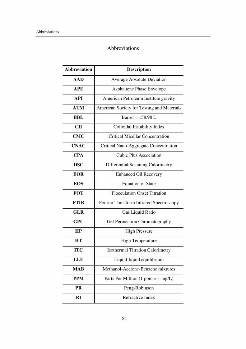
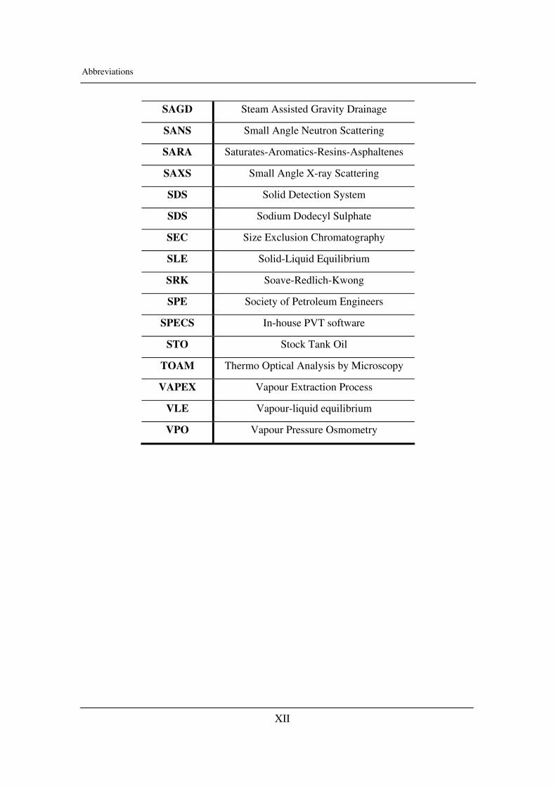
Abbreviations
Abbreviation Description
AAD Average Absolute Deviation
APE Asphaltene Phase Envelope
API American Petroleum Institute gravity
ATM American Society for Testing and Materials
BBL Barrel = 158.98 L
CII Colloidal Instability Index
CMC Critical Micellar Concentration
CNAC Critical Nano-Aggregate Concentration
CPA Cubic Plus Association
DSC Differential Scanning Calorimetry
EOR Enhanced Oil Recovery
EOS Equation of State
FOT Flocculation Onset Titration
FTIR Fourier Transform Infrared Spectroscopy
GLR Gas Liquid Ratio
GPC Gel Permeation Chromatography
HP High Pressure
HT High Temperature
ITC Isothermal Titration Calorimetry
LLE Liquid-liquid equilibrium
MAB Methanol-Acetone-Benzene mixtures
PPM Parts Per Million (1 ppm = 1 mg/L)
PR Peng-Robinson
RI Refractive Index
Abbreviations
XII
SAGD Steam Assisted Gravity Drainage
SANS Small Angle Neutron Scattering
SARA Saturates-Aromatics-Resins-Asphaltenes
SAXS Small Angle X-ray Scattering
SDS Solid Detection System
SDS Sodium Dodecyl Sulphate
SEC Size Exclusion Chromatography
SLE Solid-Liquid Equilibrium
SRK Soave-Redlich-Kwong
SPE Society of Petroleum Engineers
SPECS In-house PVT software
STO Stock Tank Oil
TOAM Thermo Optical Analysis by Microscopy
VAPEX Vapour Extraction Process
VLE Vapour-liquid equilibrium
VPO Vapour Pressure Osmometry
Definitions
XIII
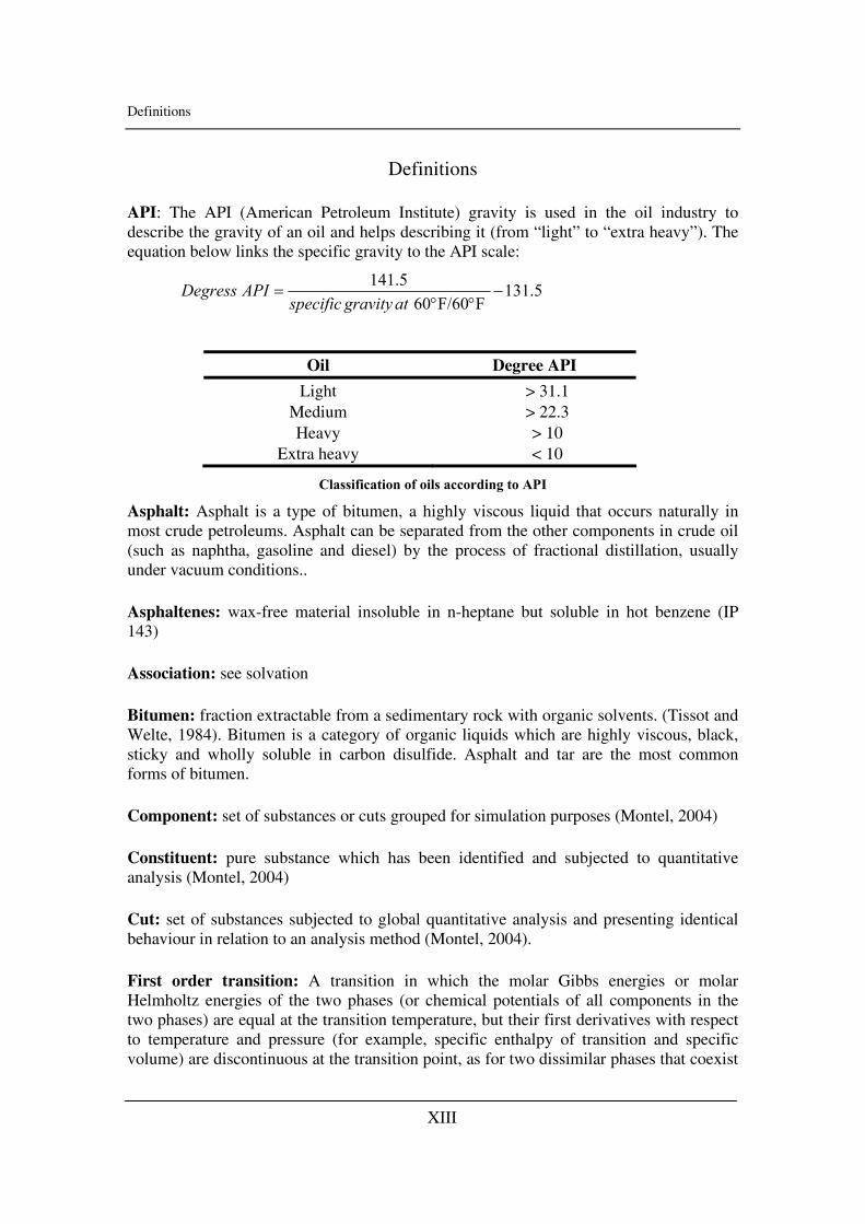
Definitions API: The API (American Petroleum Institute) gravity is used in the oil industry to describe the gravity of an oil and helps describing it (from “light” to “extra heavy”). The equation below links the specific gravity to the API scale:
5.131FF/6060
5.141−
°°=
atgravityspecificAPIDegress
Oil Degree API
Light Medium Heavy
Extra heavy
> 31.1 > 22.3 > 10 < 10
Classification of oils according to API
Asphalt: Asphalt is a type of bitumen, a highly viscous liquid that occurs naturally in most crude petroleums. Asphalt can be separated from the other components in crude oil (such as naphtha, gasoline and diesel) by the process of fractional distillation, usually under vacuum conditions.. Asphaltenes: wax-free material insoluble in n-heptane but soluble in hot benzene (IP 143) Association: see solvation Bitumen: fraction extractable from a sedimentary rock with organic solvents. (Tissot and Welte, 1984). Bitumen is a category of organic liquids which are highly viscous, black, sticky and wholly soluble in carbon disulfide. Asphalt and tar are the most common forms of bitumen. Component: set of substances or cuts grouped for simulation purposes (Montel, 2004) Constituent: pure substance which has been identified and subjected to quantitative analysis (Montel, 2004) Cut: set of substances subjected to global quantitative analysis and presenting identical behaviour in relation to an analysis method (Montel, 2004). First order transition: A transition in which the molar Gibbs energies or molar Helmholtz energies of the two phases (or chemical potentials of all components in the two phases) are equal at the transition temperature, but their first derivatives with respect to temperature and pressure (for example, specific enthalpy of transition and specific volume) are discontinuous at the transition point, as for two dissimilar phases that coexist
Definitions
XIV
and that can be transformed into one another by a change in a field variable such as pressure, temperature, magnetic or electric field (Clark et al., 1994). Flocculation: The process of adding reagents to facilitate the removal of suspended solids and colloidal particles (less than 1 micron). It is used in the final stage of solids-liquids separation for large water treatment systems, either via settling, flotation or filtration. The coagulant is the reagent that destabilized the solids and causes them to flocculate (come together and grow till they are heavy enough to sink). Glass transition: A second-order transition in which a supercooled melt yields, on cooling, a glassy structure. Below the glass-transition temperature the physical properties vary in a manner similar to those of the crystalline phase (Clark et al., 1994) Kerogen: it designates the organic constituent of the sedimentary ricks that is neither soluble in aqueous alkaline solvents nor in the common organic solvents. Sometimes, it is used for the total organic matter of sedimentary rocks but it seems to be a misuse (Tissot and Welte, 1984) Lithology: see Petrology Lyophilic: solvent loving Lyophobic: solvent hating Maltenes: mixture of the resins and oils obtained as filtrates from the asphaltene precipitation (Andersen and Speight, 2001) Oligomer: in chemistry, an oligomer consists of a finite number of monomer units ("oligo" is Greek for "a few"), in contrast to a polymer which, at least in principle, consists of an infinite number of monomers. Order-disorder transition: A transition in which the degree of order of the system changes. Three principal types of disordering transitions may be distinguished: (i) positional disordering in a solid, (ii) orientational disordering which may be static or dynamic and (iii) disordering associated with electronic and nuclear spin states (Clark et al., 1994). Petrology: it is a field of geology which focuses on the study of rocks and the conditions by which they form. There are three branches of petrology, corresponding to the three types of rocks: igneous, metamorphic, and sedimentary. Porphyrines: A porphyrin is a heterocyclic macrocycle made from 3 pyrrole subunits and one pyrroline subunit, and linked on opposite sides through 4 methine bridges. Precipitation: The formation of a solid phase within a liquid phase (Clark et al., 1994).
Definitions
XV
Pyridine: Pyridine C5H5N is a simple heterocyclic aromatic organic compound that is structurally related to benzene, with one CH group in the six-membered ring replaced by a nitrogen atom. Pyrrole: Pyrrole, or pyrrol, is a heterocyclic aromatic organic compound, a five-membered ring with the formula C4H5N. Second-order transition: A transition in which a crystal structure undergoes a continuous change and in which the first derivatives of the Gibbs energies (or chemical potentials) are continuous but the second derivatives with respect to temperature and pressure (i.e. heat capacity, thermal expansion, compressibility) are discontinuous (Clark et al., 1994). Sedimentation: Process by which solid material settles out of a suspension in a liquid medium under the opposing forces of gravitation and buoyancy. Solvation: when specific chemical forces act between molecules, there is a possibility of complex formation. The complexes cannot be isolated usually but their existence is certain from measurements such as spectroscopic studies. Hydrogen bonding is an example as well as Lewis acid/base interactions. When complexation occurs between molecules that are all from the same component, the phenomenon is called association. When complexation occurs between molecules that are from different components, the phenomenon is called solvation (Elliott and Lira, 1999). Stacking: Stacking in supramolecular chemistry refers to a stacked arrangement of aromatic molecules, which interact through aromatic interactions. The most popular example of a stacked system is found from consecutive base pairs in DNA. Thiophene: it (C4H4S) is a heterocyclic aromatic organic compound. It is aromatic because one of the two lone electron pairs of the sulfur atom contributes to the delocalized pi electron system. Wax: paraffinic waxes are n-alkanes with n greater than 17. Literature Andersen, S.I., Speight J.G., Petroleum resins: separation, character, and role in petroleum, Petroleum Science and Technology (2001), 19, 1 – 34 Clark J.B., Hastie J.W., Kihlborg L.H.E., Metselaar R., Thackeray M.M., Definitions of terms relating to phase transitions of the solid state, Pure &App. Chem. (1994), 66, 577-594 Elliott J.R., Lira C.T., Introductory chemical engineering thermodynamics, Prentice Hall PTR, Upper Saddle River, 1999
Definitions
XVI
Montel F., Petroleum Thermodynamics, Total, 2004 Tissot B.P., Welte D.H., Petroleum formation and occurrence, Second Edition, Ed. Springer-Verlag, Berlin, 1984 University of Calgary: www.ucalgary.ca/~schramm/lyophil.htm Wikipedia Encyclopaedia: www.wikipedia.com
Acknowledgments
XVII
Acknowledgments
A PhD is a long journey. It goes from painful to happy and thrilling moments,
accompanied by hopeless instants of doubts, the main questions being “what I am doing
here?” or “what is the point?”. Fortunately, one is not alone to go through this three-year
expedition.
First, I thank Professor Erling Stenby for making this PhD possible and giving me the
chance to work in such a creative and high-quality environment. I thank him for his
continuous support and his assistance.
I express my deep and sincere gratitude to Dr. Simon I. Andersen, for leading me through
the dark world of asphaltenes. His guidance, his impressive knowledge of the literature
and the friendly atmosphere he initiated transformed these three years in a very rich and
human experience. Tusind tak Simon! Jeg var meget stolt at arbejde med dig.
I would like to thank the administrative, technical and academic staff of IVC-SEP for
helping me in many different ways, especially Annelise Lerche Kofod, Anne-Louise
Biede, Zacarias Tecle or Povl Andersen to name a few. I should also express gratitude to
the two Master students I worked with, Diep Duong and Veronica Torcal-Garcia, for our
fruitful collaboration and their dedication.
I spent more than six months in Pau, at the Laboratoire des Fluides Complexes of the
University of Pau and at the TOTAL Research Centre. The various stays I had there were
incredibly rich from a scientific and personal point of view. I am grateful to all the people
who helped me there, especially to Associate Professor Hervé Carrier for his guidance,
his patience, his time and his friendship; to Professor Jean-Luc Daridon for his help and
the fruitful discussions; to Associate Professor David Bessières and Dr. Frédéric Plantier
for their priceless help in and out of the laboratory; to my fellow PhD students from Pau

Acknowledgments
XVIII
for sharing these very special moments, especially Valérie Montel, Carlos Canelon and
Michel Milhet.
I am very grateful to TOTAL for partially funding the various stays in Pau and giving me
the opportunity to work in their research centre (CSTJF, Pau) and to attend some very
useful and interesting internal courses. A very special thank to Dr. Honggang Zhou who
welcome me in his office, answered all my questions (even when he was travelling
around the world) and who always found time for me.
I cannot forget the ones sharing the daily life at DTU and in Denmark. Many of them are
now scattered all over the world. So, friends of Denmark, Argentina, Spain, Colombia,
Mexico, France, Italy, Ireland, England, Germany, Portugal, Greece and so on, I am
grateful to all of you for many different reasons. You all contributed to make these three
years a very, very special time of my life (with a special mention to Géraldine Vigan-
Guyet and Matías Monsalvo).
Last - but not least - many thoughts to my family. Thank you for supporting all the
choices I made so far. I will never be a wine-maker but I am sure you understand! A
special thought for my two nephews, Antonin and the newly arrived Alexandre.
Chapter I – Introduction to asphaltenes
1
Chapter I
Introduction to Asphaltenes
Chapter I – Introduction to asphaltenes
2
Table of Contents
1. Asphaltenes: definition, formation and characterization ..................................... 5
1.1. The definition...................................................................................................... 5
1.2. Asphaltene formation.......................................................................................... 7
1.3. Asphaltene characterization .............................................................................. 10
1.3.1. Solubility parameter of asphaltenes .......................................................... 11
1.3.2. Elemental composition.............................................................................. 12
1.3.3. Asphaltene molecules ............................................................................... 12
1.3.4. Asphaltenes in petroleum.......................................................................... 13
1.3.5. Molecular weight ...................................................................................... 15
1.3.6. Thermophysical properties........................................................................ 16
2. Asphaltenes and Aggregation ................................................................................ 17
2.1. Aggregation and intermolecular forces............................................................. 17
2.1.1. The self-association: CNAC and energies ................................................ 17
2.1.2. Van der Waals forces and aggregation ..................................................... 18
2.1.3. Charge transfer interactions and aggregation ........................................... 19
2.1.4. What about the CMC? .............................................................................. 21
2.1.5. Why is self-association not infinite?......................................................... 22
2.2. The role of resins .............................................................................................. 23
2.3. Asphaltene precipitation and flocculation ........................................................ 25
2.3.1. Theory of colloid stability......................................................................... 25
2.3.2. Asphaltene precipitation and flocculation ................................................ 30
2.3.3. When does asphaltene precipitation occur? .............................................. 33
2.3.4. The reversibility ........................................................................................ 39
2.4. Unanswered questions ...................................................................................... 40
Chapter I – Introduction to asphaltenes
3
3. Asphaltenes and Petroleum industry .................................................................... 41
3.1. The problems related to asphaltenes in the oil industry.................................... 41
3.2. A few words about the Enhanced Oil Recovery (EOR) ................................... 42
3.3. The Vapex Process............................................................................................ 43
3.4. CO2 injection..................................................................................................... 44
3.5. Which oils/fields are problematic? ................................................................... 46
3.6. What are the solutions so far?........................................................................... 46
3.6.1. Prevention ................................................................................................. 46
3.6.2. The empirical tools ................................................................................... 47
3.6.3. Remediation .............................................................................................. 49
4. Conclusion ............................................................................................................... 50
5. Aim of this project .................................................................................................. 51
Literature......................................................................................................................... 52
Chapter I – Introduction to asphaltenes
4
What are asphaltenes? How are they formed? Can they be characterized? Why do they
aggregate and what are the consequences? Why do they precipitate? What happens
during precipitation? What is the exact role of resins? Do asphaltenes in solution behave
like in crude oil? What is the difference between flocculation and precipitation?
Most of these questions have already been discussed and studied in the literature.
Nonetheless, it appears interesting to make a quick review about these issues, which are
not answered for most of them.
Chapter I – Introduction to asphaltenes
5
1. Asphaltenes: definition, formation and characterization
1.1. The definition
Let us refer to the definition given by the IP 143 standard: “the asphaltenes content of a
petroleum product is the percentage by weight of wax-free material insoluble in n-
heptane but soluble in hot benzene”.
This could seem like a clear and well-established definition but a quick look at the
Asphaltene Standardization Discussion web site - started after the 5th International
Conference on “Petroleum Phase Behaviour and Fouling” (Banff, 2004) – shows that the
very definition of asphaltenes is quite controversial:
• “I have (more or less) stopped using the term asphaltenes and instead refer to
such problems as organic depositions. At least that gives me one less problem
namely; explaining to the operational personnel how we can have asphaltene
problems with zero asphaltene content” (Per Fotland, Norsk Hydro AS, Bergen,
Norway.)
• “ASTM and other standards have directed our thinking toward standardized ways
to isolate and quantify those materials, but after many years of testing it should be
clear that what is important is not the amount of material, but its stability as a
function of temperature, pressure, and composition. The continuing focus on
separations illustrates the principal danger of standards: a poorly chosen
standard can direct attention in the wrong direction”. (Jill Buckley, PRRC, New
Mexico Tech)
These two comments summarize the questions rising even amongst experts. Why
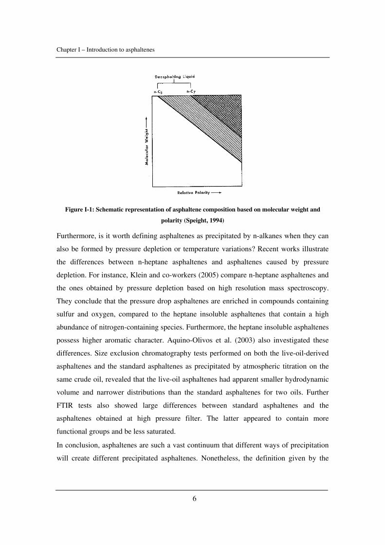
choosing n-heptane and not n-pentane? The well-known schematic representation of
Long is explicit and shows the difference between those two precipitants and how they
affect asphaltenes (Figure I-1). N-heptane asphaltenes are more polar and heavier than the
n-pentane ones.
Chapter I – Introduction to asphaltenes
6
Figure I-1: Schematic representation of asphaltene composition based on molecular weight and
polarity (Speight, 1994)
Furthermore, is it worth defining asphaltenes as precipitated by n-alkanes when they can
also be formed by pressure depletion or temperature variations? Recent works illustrate
the differences between n-heptane asphaltenes and asphaltenes caused by pressure
depletion. For instance, Klein and co-workers (2005) compare n-heptane asphaltenes and
the ones obtained by pressure depletion based on high resolution mass spectroscopy.
They conclude that the pressure drop asphaltenes are enriched in compounds containing
sulfur and oxygen, compared to the heptane insoluble asphaltenes that contain a high
abundance of nitrogen-containing species. Furthermore, the heptane insoluble asphaltenes
possess higher aromatic character. Aquino-Olivos et al. (2003) also investigated these
differences. Size exclusion chromatography tests performed on both the live-oil-derived
asphaltenes and the standard asphaltenes as precipitated by atmospheric titration on the
same crude oil, revealed that the live-oil asphaltenes had apparent smaller hydrodynamic
volume and narrower distributions than the standard asphaltenes for two oils. Further
FTIR tests also showed large differences between standard asphaltenes and the
asphaltenes obtained at high pressure filter. The latter appeared to contain more
functional groups and be less saturated.
In conclusion, asphaltenes are such a vast continuum that different ways of precipitation
will create different precipitated asphaltenes. Nonetheless, the definition given by the
Chapter I – Introduction to asphaltenes
7
IP143 method is the most commonly used one. Note that in this work, the asphaltenes
obtained from dead oils are n-heptane precipitated as described in Appendix I-1.
The whole issue of crude oil separation is also of interest. It was reported lately that the
conventional SARA separation (Saturates – Aromatics – Resins – Asphaltenes) of crude
oils - which entails preliminary “deasphaltening” and subsequent separation of the
soluble portion into Saturates, Aromatics and Resins - has inherent cross-contamination,
and inconsistencies among reporting laboratories (Bissada et al., 2005). Besides,
Andersen et al. (2001 a) submitted various crude oils to three laboratories and asked for
several analysis to be performed, including the asphaltene content. The differences in
asphaltene yields are strikingly large, with deviation factors up to 254.
Such results point out one of the difficulties related to asphaltenes and the lack of
confidence one may have with experimental data not obtained personally. How trustful is
a SARA analysis or an asphaltene content? If one works with asphaltenes precipitated by
gas injection, how worthy is it to measure molar weight on n-heptane asphaltenes? These
questions stress that the mere definition of asphaltenes is still an-going process.
Many well-documented monographs are available - Speight (1999), Yen and Chilingarian
(1994) or Sheu and Mullins (1995) for instance- and they should be consulted for further
details about the issues raised in this paragraph.
So, what is the solution if asphaltenes cannot be defined or analyzed? This will be
discussed in paragraph 1.3. But, first of all, let us try to understand how asphaltenes are
formed and in which oil they are present.
1.2. Asphaltene formation
This paragraph is mainly inspired by the book written by Tissot and Welte (Tissot and
Welte, 1984).
The structural evolution of kerogen is due to the burial (increase in temperature and
pressure). The temperature rise promotes the formation of bitumen and particularly of
hydrocarbons. One of the proposed structures of kerogen is as follows: cyclic nuclei
bearing alkyl chains and functions and linked by heteroatomic bonds and aliphatic chains.
Since the conditions are changed by the burial, this structure is not anymore in
Chapter I – Introduction to asphaltenes
8
equilibrium and, hence, rearrangements take place: the aromatization is increased and
an ordered carbon structure is developed. The stable structure under these conditions
would be graphite but this stage is never reached in non-metamorphosed sediments.
Nonetheless, the building blocks of kerogen (each nucleus made of two or more aromatic
sheets) tend to become progressively parallel.
During the diagenesis, heteroatomic bonds are broken. Heteroatoms (especially oxygen)
are partly removed as volatile compounds ( 2H O , 2CO ). The rupture of these bonds
liberates smaller structural units made of one or several bound nuclei and aliphatic
chains. The larger ones are structurally similar to kerogen but of lower molecular weight
and therefore soluble: these are the asphaltenes. Here, the MAB extracts mentioned by
Tissot and Welte, i.e. heavy bitumen extracted by Methanol-Acetone-Benzene mixtures,
are considered as asphaltenes, according to the note written page 175 (“(MAB) can be
considered as being made of heavier, or more polar, asphaltenes than those extracted by
chloroform or comparable solvents”). During this first stage (the diagenesis), the larger
fragments containing heteroatoms (asphaltenes and resins) are predominant.
As temperature continues to increase, the catagenesis starts. More bonds of various types
are broken, like esters and some C-C as well, within the kerogen and within the
previously generated fragments (asphaltenes, etc…). The new fragments become smaller
and without oxygen. This corresponds first to the principal phase of oil formation and
then to the stage of wet gas and condensate generation.
When the sediments reach the deepest part of the sedimentary basins, a general cracking
of C-C occurs, both in kerogen and bitumen. Aliphatic groups that were still present in
kerogen almost disappear. This is the principal phase of dry gas formation.
Once most labile functional groups and chains are eliminated, aromatization and
polycondensation of the residual kerogen increases. Such residual kerogen is unable to
generate hydrocarbons. This phase is called metagenesis.
Chapter I – Introduction to asphaltenes
9
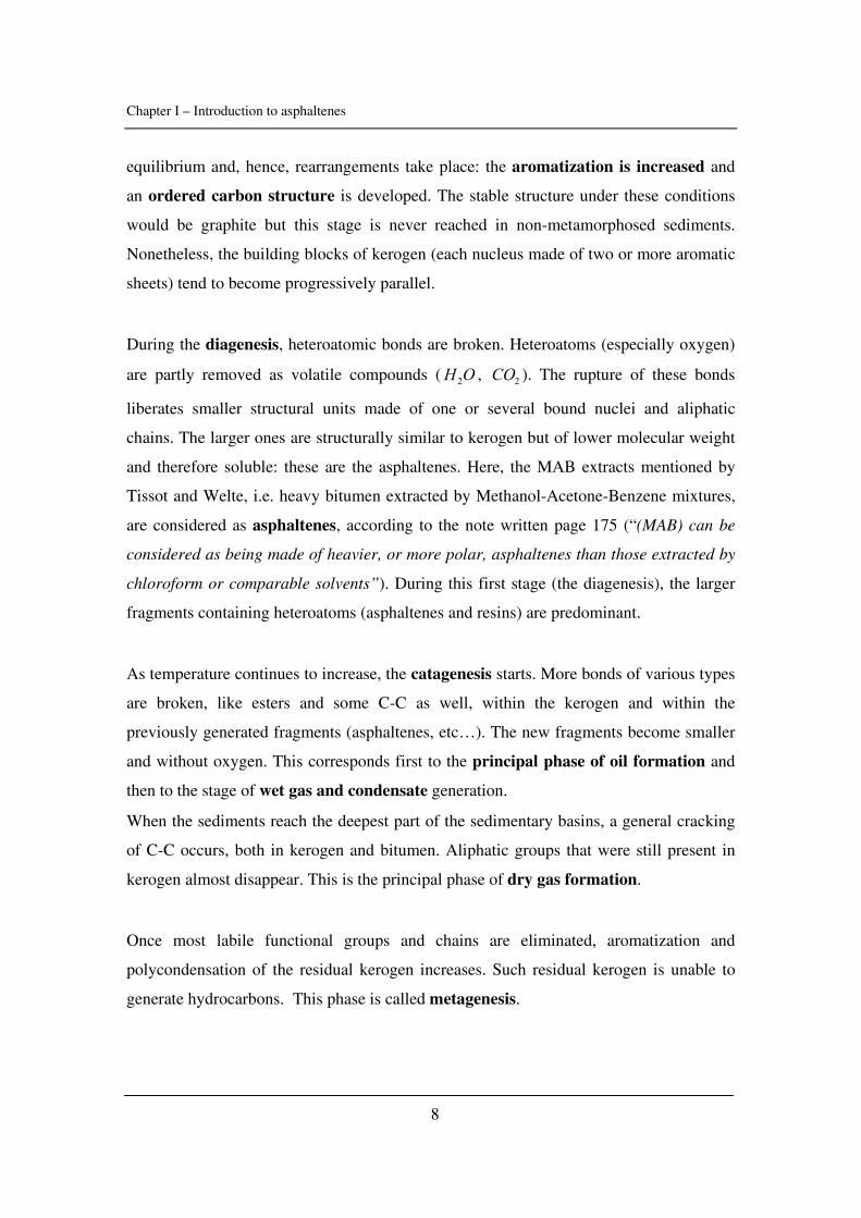
Non-hydrocarbon gases – mainly nitrogen 2N and hydrogen sulphide 2H S – may also be
generated during late catagenesis and metagenesis and they are associated with methane
and light hydrocarbons in certain basins. Hydrogen sulphide 2H S may be produced in
large amounts by thermal cracking from kerogen and from liquid-sulphur containing
compounds present in crude oils. Those two gases are of interest since they can be related
to asphaltene instability.
Figure I-2 summarizes the hydrocarbon formation.
Figure I-2: General scheme of hydrocarbon formation (Tissot and Welte, 1984)
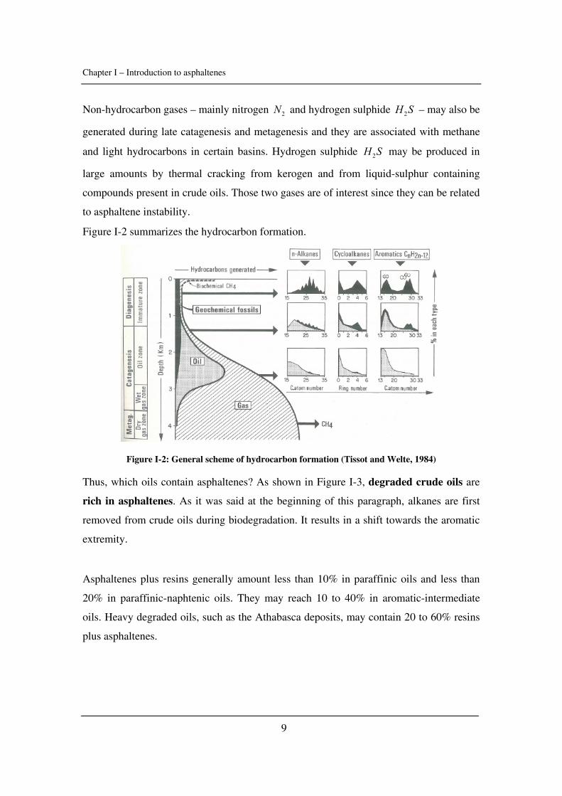
Thus, which oils contain asphaltenes? As shown in Figure I-3, degraded crude oils are
rich in asphaltenes. As it was said at the beginning of this paragraph, alkanes are first
removed from crude oils during biodegradation. It results in a shift towards the aromatic
extremity.
Asphaltenes plus resins generally amount less than 10% in paraffinic oils and less than
20% in paraffinic-naphtenic oils. They may reach 10 to 40% in aromatic-intermediate
oils. Heavy degraded oils, such as the Athabasca deposits, may contain 20 to 60% resins
plus asphaltenes.
Chapter I – Introduction to asphaltenes
10
Figure I-3: Ternary diagram showing the composition of the six classes of crude oils from 541 oil
fields (Tissot and Welte, 1984)
But, does it matter that much to know how much asphaltenes a crude oil contain from a
production point of view? It is well-known that the asphaltene-rich oils are quite stable
with respect to asphaltene precipitation. Andersen and co-workers studied several fields
from Venezuela where 20 to 50 ppm were enough to cause asphaltene precipitation
(Andersen et al., 2001). Per Fotland summarizes it all when he writes that “we can have
asphaltene problems with zero asphaltene content”. This issue will be further discussed
in paragraph 3.5.
1.3. Asphaltene characterization
How can a molecule be characterized if its extraction is problematic and gives rise to
uncertainties about its nature? What is the validity of such an analysis? This might be the
most difficult dilemma about asphaltenes: extracting them from the crude oil will modify
them. During the workshop about asphaltene standardization of the 5th International
Conference on Petroleum Phase Behaviour and Fouling (Banff, 2004), Stig Friberg,
recognized and awarded expert in colloidal science, suggested that asphaltenes should
stay “where they are” and should be studied in situ if any results were expected. Though
Chapter I – Introduction to asphaltenes
11
this idea is very tempting, the millions of compounds present in crude oil make it difficult
to obtain relevant data when asphaltenes are studied in situ. In this paragraph, several
aspects of asphaltenes such as its molecular weights, composition, structure or
thermophysical properties will be briefly described and commented in order to give a
quick overview of the nature of asphaltenes
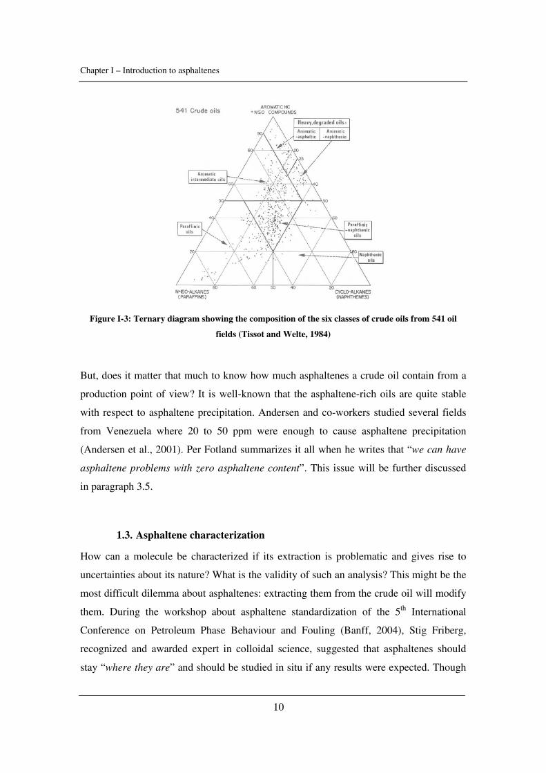
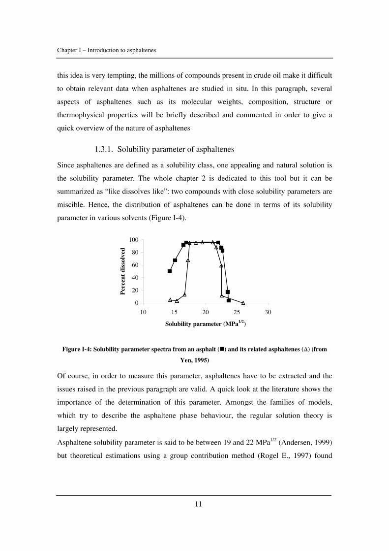
1.3.1. Solubility parameter of asphaltenes
Since asphaltenes are defined as a solubility class, one appealing and natural solution is
the solubility parameter. The whole chapter 2 is dedicated to this tool but it can be
summarized as “like dissolves like”: two compounds with close solubility parameters are
miscible. Hence, the distribution of asphaltenes can be done in terms of its solubility
parameter in various solvents (Figure I-4).
0
20
40
60
80
100
10 15 20 25 30
Solubility parameter (MPa1/2)
Per
cent
dis
solv
ed
Figure I-4: Solubility parameter spectra from an asphalt ( ) and its related asphaltenes (∆) (from
Yen, 1995)
Of course, in order to measure this parameter, asphaltenes have to be extracted and the
issues raised in the previous paragraph are valid. A quick look at the literature shows the
importance of the determination of this parameter. Amongst the families of models,
which try to describe the asphaltene phase behaviour, the regular solution theory is
largely represented.
Asphaltene solubility parameter is said to be between 19 and 22 MPa1/2 (Andersen, 1999)
but theoretical estimations using a group contribution method (Rogel E., 1997) found
Chapter I – Introduction to asphaltenes
12
means values between 23.1 and 26.4 MPa1/2, depending on the molar weight. More
details are available in Chapter 2, Paragraph 3.
1.3.2. Elemental composition
The choice of the precipitant and the procedure used are obviously important. For
instance the H/C ratios of the n-heptane precipitate are much lower than those of the
pentane precipitate, i.e. the heptane precipitate has a higher degree of aromaticity
(Speight, 1994). Major differences are also observable with the N/C, O/C and S/C ratios.
Asphaltene fraction contains the largest percentage of heteroatoms (N, S, O) and
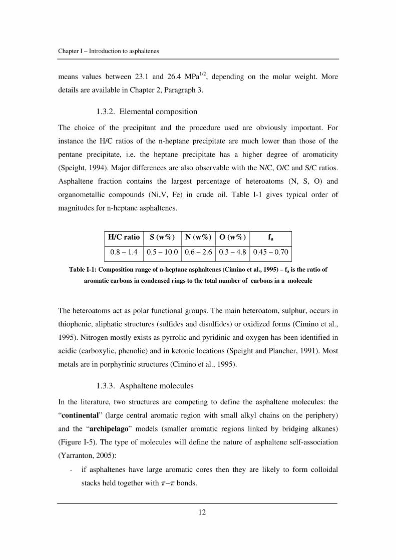
organometallic compounds (Ni,V, Fe) in crude oil. Table I-1 gives typical order of
magnitudes for n-heptane asphaltenes.
H/C ratio S (w%) N (w%) O (w%) fa
0.8 – 1.4 0.5 – 10.0 0.6 – 2.6 0.3 – 4.8 0.45 – 0.70
Table I-1: Composition range of n-heptane asphaltenes (Cimino et al., 1995) – fa is the ratio of
aromatic carbons in condensed rings to the total number of carbons in a molecule
The heteroatoms act as polar functional groups. The main heteroatom, sulphur, occurs in
thiophenic, aliphatic structures (sulfides and disulfides) or oxidized forms (Cimino et al.,
1995). Nitrogen mostly exists as pyrrolic and pyridinic and oxygen has been identified in
acidic (carboxylic, phenolic) and in ketonic locations (Speight and Plancher, 1991). Most
metals are in porphyrinic structures (Cimino et al., 1995).
1.3.3. Asphaltene molecules
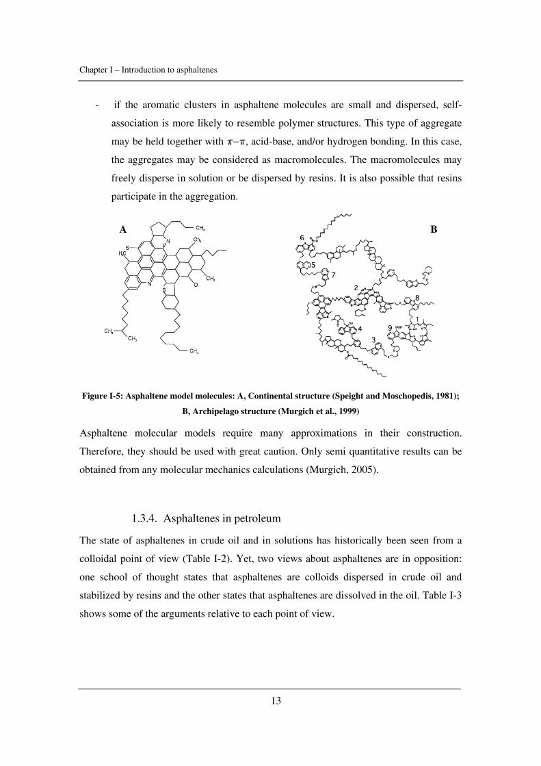
In the literature, two structures are competing to define the asphaltene molecules: the
“continental” (large central aromatic region with small alkyl chains on the periphery)
and the “archipelago” models (smaller aromatic regions linked by bridging alkanes)
(Figure I-5). The type of molecules will define the nature of asphaltene self-association
(Yarranton, 2005):
- if asphaltenes have large aromatic cores then they are likely to form colloidal
stacks held together with π−π bonds.
Chapter I – Introduction to asphaltenes
13
- if the aromatic clusters in asphaltene molecules are small and dispersed, self-
association is more likely to resemble polymer structures. This type of aggregate
may be held together with π−π, acid-base, and/or hydrogen bonding. In this case,
the aggregates may be considered as macromolecules. The macromolecules may
freely disperse in solution or be dispersed by resins. It is also possible that resins
participate in the aggregation.
Figure I-5: Asphaltene model molecules: A, Continental structure (Speight and Moschopedis, 1981);
B, Archipelago structure (Murgich et al., 1999)
Asphaltene molecular models require many approximations in their construction.
Therefore, they should be used with great caution. Only semi quantitative results can be
obtained from any molecular mechanics calculations (Murgich, 2005).
1.3.4. Asphaltenes in petroleum
The state of asphaltenes in crude oil and in solutions has historically been seen from a
colloidal point of view (Table I-2). Yet, two views about asphaltenes are in opposition:
one school of thought states that asphaltenes are colloids dispersed in crude oil and
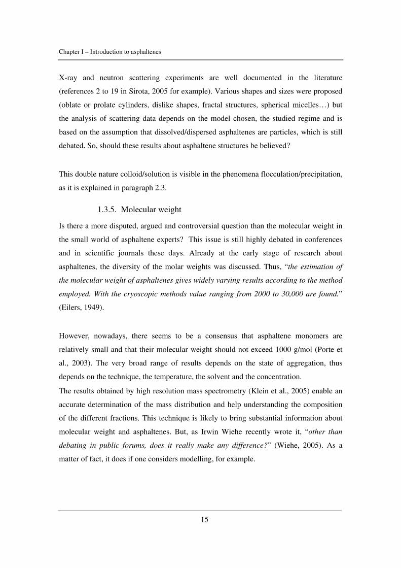
stabilized by resins and the other states that asphaltenes are dissolved in the oil. Table I-3
shows some of the arguments relative to each point of view.
A B
Chapter I – Introduction to asphaltenes
14
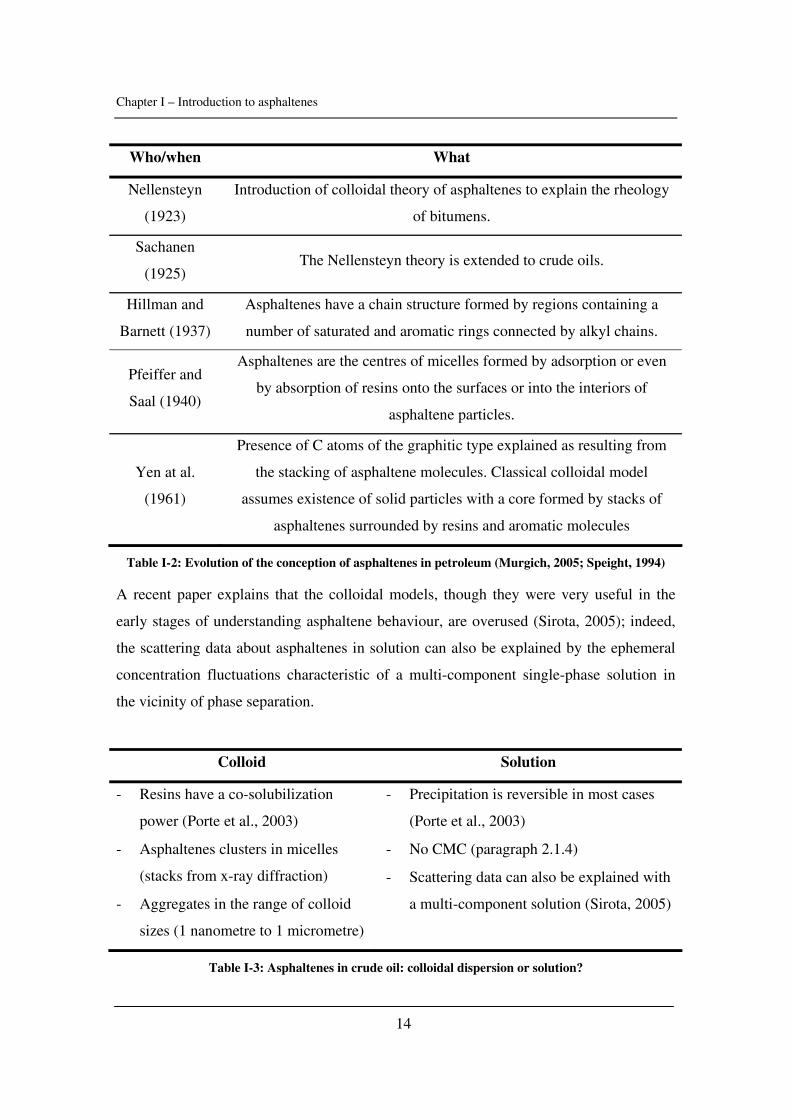
Who/when What
Nellensteyn
(1923)
Introduction of colloidal theory of asphaltenes to explain the rheology
of bitumens.
Sachanen
(1925) The Nellensteyn theory is extended to crude oils.
Hillman and
Barnett (1937)
Asphaltenes have a chain structure formed by regions containing a
number of saturated and aromatic rings connected by alkyl chains.
Pfeiffer and
Saal (1940)
Asphaltenes are the centres of micelles formed by adsorption or even
by absorption of resins onto the surfaces or into the interiors of
asphaltene particles.
Yen at al.
(1961)
Presence of C atoms of the graphitic type explained as resulting from
the stacking of asphaltene molecules. Classical colloidal model
assumes existence of solid particles with a core formed by stacks of
asphaltenes surrounded by resins and aromatic molecules
Table I-2: Evolution of the conception of asphaltenes in petroleum (Murgich, 2005; Speight, 1994)
A recent paper explains that the colloidal models, though they were very useful in the
early stages of understanding asphaltene behaviour, are overused (Sirota, 2005); indeed,
the scattering data about asphaltenes in solution can also be explained by the ephemeral
concentration fluctuations characteristic of a multi-component single-phase solution in
the vicinity of phase separation.
Colloid Solution
- Resins have a co-solubilization
power (Porte et al., 2003)
- Asphaltenes clusters in micelles
(stacks from x-ray diffraction)
- Aggregates in the range of colloid
sizes (1 nanometre to 1 micrometre)
- Precipitation is reversible in most cases
(Porte et al., 2003)
- No CMC (paragraph 2.1.4)
- Scattering data can also be explained with
a multi-component solution (Sirota, 2005)
Table I-3: Asphaltenes in crude oil: colloidal dispersion or solution?
Chapter I – Introduction to asphaltenes
15
X-ray and neutron scattering experiments are well documented in the literature
(references 2 to 19 in Sirota, 2005 for example). Various shapes and sizes were proposed
(oblate or prolate cylinders, dislike shapes, fractal structures, spherical micelles…) but
the analysis of scattering data depends on the model chosen, the studied regime and is
based on the assumption that dissolved/dispersed asphaltenes are particles, which is still
debated. So, should these results about asphaltene structures be believed?
This double nature colloid/solution is visible in the phenomena flocculation/precipitation,
as it is explained in paragraph 2.3.
1.3.5. Molecular weight
Is there a more disputed, argued and controversial question than the molecular weight in
the small world of asphaltene experts? This issue is still highly debated in conferences
and in scientific journals these days. Already at the early stage of research about
asphaltenes, the diversity of the molar weights was discussed. Thus, “the estimation of
the molecular weight of asphaltenes gives widely varying results according to the method
employed. With the cryoscopic methods value ranging from 2000 to 30,000 are found.”
(Eilers, 1949).
However, nowadays, there seems to be a consensus that asphaltene monomers are
relatively small and that their molecular weight should not exceed 1000 g/mol (Porte et
al., 2003). The very broad range of results depends on the state of aggregation, thus
depends on the technique, the temperature, the solvent and the concentration.
The results obtained by high resolution mass spectrometry (Klein et al., 2005) enable an
accurate determination of the mass distribution and help understanding the composition
of the different fractions. This technique is likely to bring substantial information about
molecular weight and asphaltenes. But, as Irwin Wiehe recently wrote it, “other than
debating in public forums, does it really make any difference?” (Wiehe, 2005). As a
matter of fact, it does if one considers modelling, for example.
Chapter I – Introduction to asphaltenes
16
1.3.6. Thermophysical properties
There has been little work done on the thermophysical properties of asphaltenes. The
most studied properties might be the solubility parameter and the density though. Both
were determined experimentally or by molecular simulation. As it was said in paragraph
1.3.1, the solubility parameter of asphaltene has been reported between 19 and 26 MPa1/2.
The density is usually measured with a pycnometer and assuming that there is no excess
volume. Recent values were reported between 1.17 and 1.52 g/cm3 (Rogel and
Carbognani, 2003), pointing out that the smaller the ratio H/C, the higher the density. In
this study, it was also found that asphaltenes from unstable crude oils and deposits exhibit
higher densities, lower hydrogen-to-carbon ratios, and higher aromaticities than
asphaltenes from stable crude oils. Since density is strongly linked to the solubility
parameter, this is not surprising.
Diallo et al. (2000) used molecular dynamic simulations and managed to estimate most of
thermodynamic properties (molar volumes, solubility parameter, heat capacity or thermal
expansivity).
Dielectric properties of asphaltenes were also investigated (Sheu et al., 1994; Pedersen,
2000). Pedersen determined static values of permittivity (dielectric constant) for various
types of asphaltenes ranging between 2.48 and 2.71 at 298.15 K. He also calculated
dipole moments for one type of asphaltene at 333.15 K as a function of the state of
aggregation. Dipole moments could vary between 2 and 20 D.
Chapter I – Introduction to asphaltenes
17
2. Asphaltenes and Aggregation
Aggregation strongly affects asphaltenes: self-association, flocculation, precipitation,
interaction with resins. This paragraph gives a brief overview of these phenomena.
2.1. Aggregation and intermolecular forces
“A most important physical property of colloidal dispersions is the tendency of the
particles to aggregate. Encounters between particles dispersed in liquid media occur
frequently and the stability of a dispersion is determined by the interaction between the
particles during these encounters. […] The overall situation is often very complicated”
(Shaw, 1992). In this paragraph, the relative importance of intermolecular forces in the
asphaltene aggregation process is studied and their relationships to stability.
It is important to understand that aggregation affects asphaltenes at several levels:
- First, asphaltene monomers self-associate. Hydrogen bonds are mainly
responsible for such aggregation.
- Then, flocculation and precipitation are due to the aggregation of these
“macro-molecules” constituted of aggregated asphaltene monomers.
Dispersion is the key force in this process.
A short summary about intermolecular forces is available in Appendix I-2.
2.1.1. The self-association: CNAC and energies
As VPO (Vapour Pressure Osmometry) and ITC (Isothermal Titration Calorimetry)
measurements showed it (Wiehe, 2005; Merino-Garcia, 2003), aggregation starts at very
low concentration and it is almost impossible to study the monomer since the forces
driving the aggregation are quite strong. As it was mentioned in a recent paper (Porte et
al., 2003), “if the aggregation was driven by weak dispersion forces, the aggregates in
solution would coexist with a noticeable concentration of free single molecules. […]
Aggregation is induced by strong specific interactions (hydrogen bonds, for instance)”.
One can wonder when aggregation starts. Merino-Garcia (2003) found that aggregation
started before 34 ppm by means of calorimetry measurements of asphaltenes in toluene
solutions. The Critical Nano-Aggregate Concentration (CNAC) was found to be
Chapter I – Introduction to asphaltenes
18
around 100 ppm for asphaltenes in toluene by high-Q ultrasonic measurements
(Andreatta et al., 2005). However, in these measurements, the break in ultrasonic velocity
can be subject to discussion because it is of noise level. Nonetheless, absorbance
measurements in toluene seem to corroborate these results since self-association was
found to start around 100 ppm (Castillo et al., 2001). Be that as it may, one can
conclude that self-association starts at very low concentration and that asphaltene
monomers are hardly found in solution. Thus, the properties of asphaltenes are the ones
of the aggregates, as the VPO measurements clearly show it even below 100 ppm
(Wiehe, 2005).
All these measurements were done in solutions and note in crude oils. The presence of
other compounds would make it difficult to detect any change or variation. For
calorimetry, for instance, Merino-Garcia (2003) found quite low energies of interactions
(from -0.6 to -7.6 kJ/mol). He used a step-wise growth mechanism and assumed a
molar weight of 1000 g/mol. This is less than hydrogen bonding (between -10 and -40
kJ/mol). The presence of other compounds in much higher proportions would hide the
self-association phenomenon. In Merino-Garcia’s work, it was also suggested that a
fraction of asphaltenes could be inactive and, thus, it could explain this low energy. SEC
analysis of heptane-toluene fractions asphaltenes indicated that a fraction could be
inactive in the self-association process (Andersen, 1994). Besides, Merino-Garcia
assumed that the interaction asphaltene-toluene was negligible compared to the
interaction asphaltene-asphaltene. It may also account for the low energy of interaction.
To conclude, self-association starts at very low concentrations and hydrogen bonding are
believed to be mainly responsible.
2.1.2. Van der Waals forces and aggregation
Amongst the van der Waals forces, dispersion forces are believed to be responsible of
the flocculation and the precipitation processes. Each of these forces will be briefly
reviewed.
Chapter I – Introduction to asphaltenes
19
- Dispersion forces
Murgich (Murgich, 1992) claims that dispersion forces are responsible for aggregation.
However, as it was mentioned at the beginning of this paragraph, self-association is rather
driven by strong interaction forces. These forces are likely to be predominant during
flocculation and precipitation, as it is seen in paragraph 2.3.
- Induction forces
They are generally small and never exceed 7% of the total forces (Kontogeorgis, 2005).
This contribution is especially small when there are no ions or charged particles present
in the system, which is the case in asphaltenes aggregates.
- Electrostatic forces
There are several ways to represent the molecular charge distribution. One of them is
called the multipolar expansion and contains a monopole that reflects the total net charge
plus a dipole, a quadrupole and higher multipoles (Israelachvili, 1991). The dipole
moment gives a quick estimate of the polarity of a molecule. Polar forces are significant
when the dipole moment is larger than 1 D (Kontogeorgis, 2005). A few experimental
determinations of the dipole moment were done: it was found between 2.5 and 5 D
(Maruska and Rao, 1987) and between 2 and 20 D depending on the state of aggregation
(Pedersen, 2000). Pedersen also observed a clear relationship between stability in
production and polarity for toluene solutions: asphaltenes from unstable crude oils were
more polar than asphaltenes from crude oils without precipitation problems. Hence, it
seems that not only the dispersion forces play a part during flocculation and precipitation.
Amongst the van der Waals forces, dispersion and electrostatic forces seem to play a
key role in terms of aggregation.
2.1.3. Charge transfer interactions and aggregation
First, let us investigate the role of hydrogen bonding. Moschopedis and Speight
(Moschopedis and Speight, 1976) demonstrated that the asphaltene and resin fractions of
Athabasca bitumen participate in hydrogen-bonding interactions. The role of hydrogen
bonding between asphaltene and resins was also outlined by Merino-Garcia (Merino-
Chapter I – Introduction to asphaltenes
20
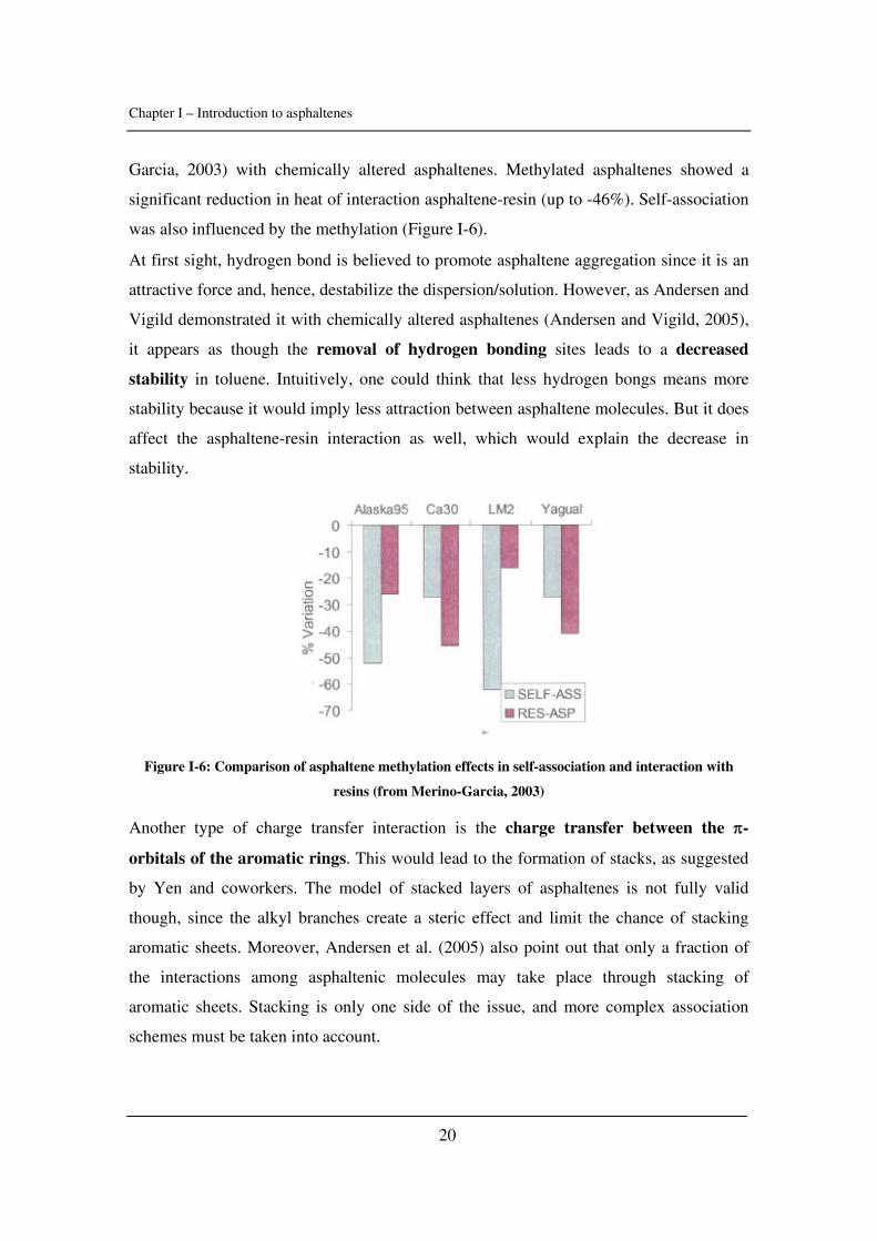
Garcia, 2003) with chemically altered asphaltenes. Methylated asphaltenes showed a
significant reduction in heat of interaction asphaltene-resin (up to -46%). Self-association
was also influenced by the methylation (Figure I-6).
At first sight, hydrogen bond is believed to promote asphaltene aggregation since it is an
attractive force and, hence, destabilize the dispersion/solution. However, as Andersen and
Vigild demonstrated it with chemically altered asphaltenes (Andersen and Vigild, 2005),
it appears as though the removal of hydrogen bonding sites leads to a decreased
stability in toluene. Intuitively, one could think that less hydrogen bongs means more
stability because it would imply less attraction between asphaltene molecules. But it does
affect the asphaltene-resin interaction as well, which would explain the decrease in
stability.
Figure I-6: Comparison of asphaltene methylation effects in self-association and interaction with
resins (from Merino-Garcia, 2003)
Another type of charge transfer interaction is the charge transfer between the π-
orbitals of the aromatic rings. This would lead to the formation of stacks, as suggested
by Yen and coworkers. The model of stacked layers of asphaltenes is not fully valid
though, since the alkyl branches create a steric effect and limit the chance of stacking
aromatic sheets. Moreover, Andersen et al. (2005) also point out that only a fraction of
the interactions among asphaltenic molecules may take place through stacking of
aromatic sheets. Stacking is only one side of the issue, and more complex association
schemes must be taken into account.
Chapter I – Introduction to asphaltenes
21
Electron transfer between the organic solid particles and the liquid organic phase
has been mentioned as well (Siffert et al., 1994). They concluded that the more intense
the transfers, the higher the charge of the particle and the better the stability of the
suspension. This type of interaction is repulsive in this case and a higher repulsive force
would improve stability.
As a conclusion, hydrogen bonds, dispersion, polar forces and π π− stacking are the key
forces in terms of aggregation. Nonetheless, only qualitative information has been found
so far with asphaltenes. As Prausnitz et al. (1999) clearly state it, “we must recognize at
the outset that our understanding of intermolecular forces is far from complete and that
quantitative results have been obtained for only simple and idealized models of real
matters”. Asphaltenes are not known to be simple and idealized molecules.
2.1.4. What about the CMC?
The “CMC” (Critical Micellar Concentration) initially observed in literature by
calorimetry (Andersen and Birdi, 1991) and surface tension (Rogacheva et al., 1980;
Rogel et al., 2000) was an appealing idea supporting the concept of micellization to
explain asphaltene aggregation.
The CMC value is between 2 and 4 g/L. Roux et al. (2001) report a change in the
aggregate size for a volume fraction larger than 4% (say 5% in mass fraction, i.e. 50 g/L!)
Ravey et al. (1988) observed a similar change in their SANS data when the asphaltene
weight fraction was larger than 2.3% in THF. These changes cannot be attributed to the
CMC. Roux and co-workers propose that the change in size is due to the interpenetration
of aggregates. Indeed, when increasing the concentration, the aggregates are forces to
come closer to each other (not energetically favourable). Thus rearrangement of
aggregates will take place: many surfactants structures go from small micelles to long
cylinders to large liposomes as the surfactant content increases above about 10% weight
(Israelachvili, 1991).
So, what does happen between 2 and 4 g/L? Which phenomenon is responsible for the
“pseudo-CMC”? Andreatta et al. (2005) conclude their paper saying that the reported
CMC’s - much higher than the CNAC’s - are probably representing some higher order
Chapter I – Introduction to asphaltenes
22
aggregation. The following points bring some interesting input about the “CMC of
asphaltenes” and make this concept slightly wobbly:
- Andersen et al. (2001 b) pointed out an interesting issue when they measured the
influence of water on these CMC measurements. Their calorimetric titrations
showed that the critical micelle concentration was highly affected by water in
such a way that it must be assumed that water plays a major role in the association
process.
- Sztukowski et al. (2003) could not detect any change in slope on a plot of
interfacial tension versus log asphaltene concentration.
- The addition of resins (petroleum polar components) to the asphaltene system was
found to eliminate the break in the curve previously assigned to CMC (Andersen
et al., 2001 b).
Instead of the micellization process, asphaltene self-association rather seems to be a step-
wise process (Merino-Garcia and Andersen, 2005). As for the “measured” CMC, if any,
it is likely not to be due to the sole asphaltene structure.
2.1.5. Why is self-association not infinite?
Roux et al. (2001) used SANS measurements on asphaltene-toluene solutions, varying the
asphaltene concentration. The molecular weight is stable from 0.3 to 3-4 % (volume
fraction) and is around 105 g/mol, which means an aggregation number of 100. When the
concentration is larger than 4%, the molecular weight is decreasing, which is due to
repulsive forces between the aggregates.
Are chemical forces able to explain this “saturated” behaviour? The saturated nature of
chemical forces is intimately connected with the theory of the covalent bond: once two
hydrogen atoms met and have formed H2, they are “satisfied” (or saturated). On the other
hand, the purely physical force between two argon molecules, for instance, does not
know such satisfaction (Prausnitz et al., 1999).
Porte et al (2003) also suggest that the morphology and structure of the aggregates is
the key rather than the saturation of chemical forces. From scattering data, they first
concluded that the dimension of the aggregates was 2 (topic that is briefly discussed in
Chapter I – Introduction to asphaltenes
23
paragraph 1.3.4). Then, the structure cannot be a fractal one since it would induce an
irreversible precipitation. Here, infinite aggregation is stopped by the high bending
flexibility of monomolecular sheets, which would sphere up and form finite vesicles. But,
as they pointed it out, there is no evidence that this vesicle model is valid.
Another option to explain the limited size of aggregates - supporting this time the
description of asphaltene aggregates as stacked sheets - is the steric hindrance. It is often
advocated to be a limiting factor in the size of asphaltenes. It was suggested lately that
petroleum asphaltenes have alkyl chains that act as steric hindrance for the self-
association (Carbognani, 2003). These alkyl branches would limit the number of sheets
per aggregate.
2.2. The role of resins
Resins and asphaltenes are usually distinguished based on the separation procedure.
However, there are several ways of preparing resins and asphaltenes, resulting in slightly
different compositions. Precipitation by propane separates resins and asphaltenes from
the rest of the crude oil, then precipitation by n-pentane or n-heptane separates resins
(soluble) from asphaltenes (insoluble) (Tissot and Welte, 1984, p 404). Resins have
longer alkyl chains and smaller aromatic rings, which make them more soluble in
aliphatic solvents and VPO measurements are a good tool to determine their monomeric
molecular weight. VPO gave results ranging between 600 and 1000 g/mol (Speight,
1999). On the other hand, asphaltenes and resins have recently been considered an almost
continuous spectrum of different polyaromatic species, each of them having its own
solubility parameter (Porte et al., 2003)
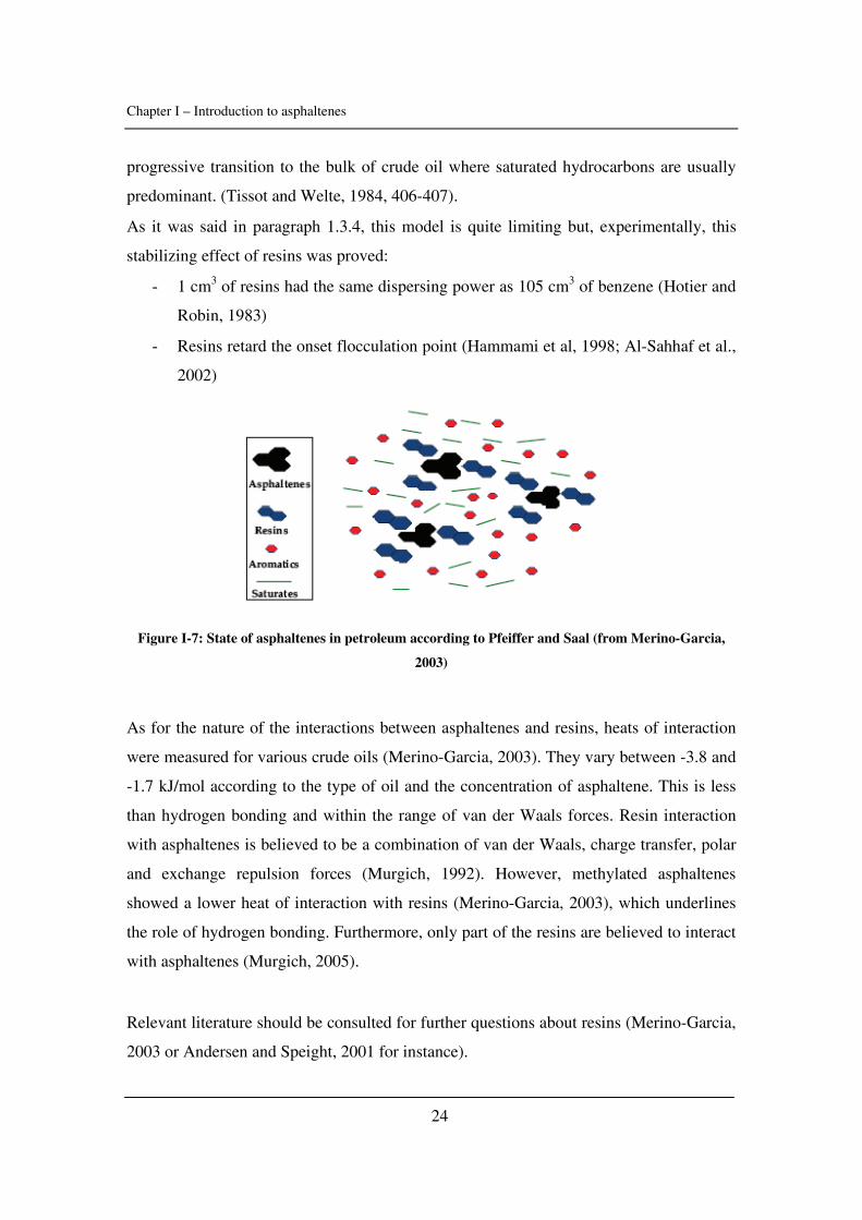
The model developed by Pfeiffer and Saal in 1940 claims that asphaltenes are dispersed
by the action of resins (Figure I-7). Resin-asphaltene interactions, especially through
hydrogen bonding, are preferred to asphaltene association and thus they would keep these
particles in suspension. The overall structure would be of a micellar type: the core of
micelle is occupied by one or several asphaltene “molecules” and is surrounded by
interacting resins. Then, resins are surrounded by aromatic hydrocarbons which ensure a
Chapter I – Introduction to asphaltenes
24
progressive transition to the bulk of crude oil where saturated hydrocarbons are usually
predominant. (Tissot and Welte, 1984, 406-407).
As it was said in paragraph 1.3.4, this model is quite limiting but, experimentally, this
stabilizing effect of resins was proved:
- 1 cm3 of resins had the same dispersing power as 105 cm3 of benzene (Hotier and
Robin, 1983)
- Resins retard the onset flocculation point (Hammami et al, 1998; Al-Sahhaf et al.,
2002)
Figure I-7: State of asphaltenes in petroleum according to Pfeiffer and Saal (from Merino-Garcia,
2003)
As for the nature of the interactions between asphaltenes and resins, heats of interaction
were measured for various crude oils (Merino-Garcia, 2003). They vary between -3.8 and
-1.7 kJ/mol according to the type of oil and the concentration of asphaltene. This is less
than hydrogen bonding and within the range of van der Waals forces. Resin interaction
with asphaltenes is believed to be a combination of van der Waals, charge transfer, polar
and exchange repulsion forces (Murgich, 1992). However, methylated asphaltenes
showed a lower heat of interaction with resins (Merino-Garcia, 2003), which underlines
the role of hydrogen bonding. Furthermore, only part of the resins are believed to interact
with asphaltenes (Murgich, 2005).
Relevant literature should be consulted for further questions about resins (Merino-Garcia,
2003 or Andersen and Speight, 2001 for instance).
Chapter I – Introduction to asphaltenes
25
2.3. Asphaltene precipitation and flocculation
In this paragraph, a short introduction about colloid stability will be given as well as the
difference between flocculation and precipitation and the particularities of asphaltene
precipitation. But, it is important to define the difference between these processes here:
- Flocculation is a state of aggregation. Asphaltenes aggregates interact within
each other and form “super aggregates”. Flocculation is not a phase transition.
Flocculation is rather related to colloids and colloidal stability than to
thermodynamics and solubility.
- Precipitation occurs when gravity overcomes Brownian forces. The “super
aggregates” are too heavy to stay in solution and, hence, they separate from the
solvent phase. It is a phase separation and it can be explained in terms of
solubility.
Therefore, the double nature of asphaltenes “dispersion/solution” introduced in paragraph
1.3.4 is present at this point.
2.3.1. Theory of colloid stability
Colloids can be broadly divided into two classes (Cooper, 2005):
- Lyophilic (solvent loving)
o Easily dispersed by the addition of a suitable dispersing medium.
o Usually thermodynamically stable and ΔG of formation is negative.
- Lyophobic, (solvent hating)
o Require vigorous mechanical agitation to be dispersed.
o Thermodynamically unstable, but are often metastable due to charge
stabilisation through the presence of surface charges.
Colloid stability is a balance between attractive and repulsive forces: when particles
collide, if the attractive forces are stronger, they aggregate and dispersion may
destabilize. When repulsive forces dominate, the system will remain in a dispersed state.
In general, the principal cause of aggregation is the van der Waals attractive forces
between the particles, which are long-range forces. To counteract these and promote
Chapter I – Introduction to asphaltenes
26
stability, equally long-range forces are necessary. The principal stabilising options are
electrostatic (the overlap of similarly charged electric double layers) and polymeric
(steric stabililisation) (Shaw, 1992)
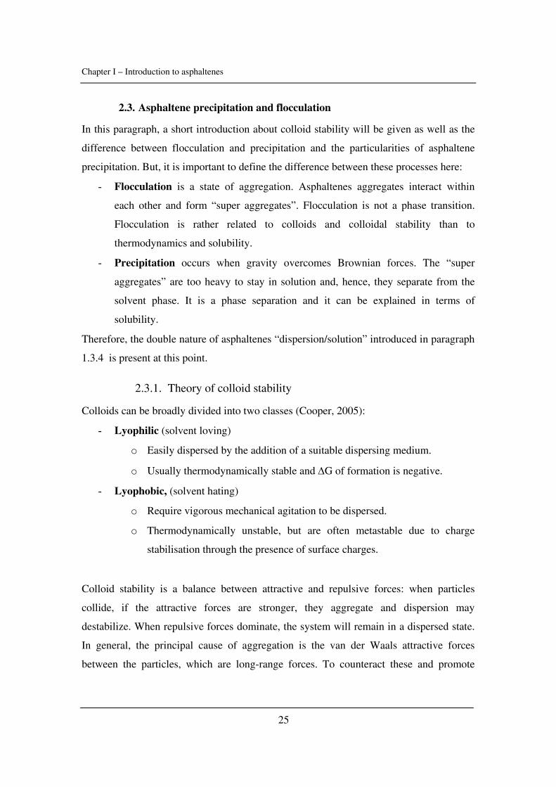
If one only considers the double-layer as source of repulsion forces, the total interaction
energy is the sum of attractive forces (van der Waals forces for instance with the potential
energy AV ) and repulsive forces (the double layer interaction with the potential energy
RV ) and can be plotted as shown in Figure I-8:
Figure I-8: Total interaction energy curve (from Shaw, 1992)
The system is stable if the potential energy maximum is large compared with the
thermal energy kT of the particles. In the case of Figure I-8, the curve V2 would be
related to an unstable system contrary to the curve V1. However, in many cases, steric
stabilisation plays a role, especially when macromolecules are adsorbed. Quoting Shaw
(Shaw, 1992): “The adsorbed layers between the particles may interpenetatre and give a
local increase in the concentration of polymer segments. Depending on the balance
between polymer-polymer and polymer-dispersion medium interactions, this may lead to
either repulsion or attraction.[…] If the dispersion medium is a good solvent for lyophilic
moieties of the adsorbed polymer, interpenetration is not favoured and interparticle
repulsion results […]. If the dispersion medium is a poor solvent, interpenetration is
favoured and attraction results. The free energy change which takes place when polymer
VR(1)
VR(2)
VA
V2
V1
Distance between particles
Chapter I – Introduction to asphaltenes
27
chains interpenetrate is influenced by factors such as temperature, pressure and solvent
composition. The point at which this free energy change is equal to zero is known at the
θ (theta)-point”. If one reads “resins” instead of “polymers”, it becomes quite familiar
with the situation of asphaltenes. This is why the colloidal view of asphaltenes has been
so popular over the years.
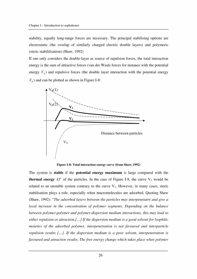
When the steric effects are added to the total interaction energy - the sum of the attractive
terms AV and the repulsive forces (electrostatic RV and steric interactions SV ) – the
potential presented in Figure I-9 can be obtained.
Figure I-9: Schematic interaction energy diagrams for sterically stabilised particles: a) in the absence
of electric double layer repulsion; b) with electric double layer repulsion (from Shaw, 1992)
Steric interactions make the entry into a deep primary minimum virtually impossible.
An easy way to discuss the effect of temperature on stability is to study the definition of
the Gibbs energy G H T SΔ = Δ − Δ as Napper suggested it (1977):
- If HΔ and SΔ are both positive and H T SΔ > Δ , the enthalpy change on close
approach opposes flocculation (flocculation is an unstable state so with 0GΔ < )
whereas entropy promotes it. Because the enthalpic contribution is dominant, this
VA + VR
VA + VR + VS
VS
Distance between particles
b)
a)
Chapter I – Introduction to asphaltenes
28
is called an enthalpic stabilisation. When T is increased, the entropic effect
becomes more and more important and the system flocculates.
- If HΔ and SΔ are both negative and H T SΔ < Δ , this is the opposite situation:
entropy favours the stability and enthalpy the flocculation. Here, flocculation
occurs when T is decreased. This is an entropic stabilisation.
- The third scenario takes place when HΔ is positive and SΔ negative. Here, they
cancel their opposite effects and, in theory, no temperature variation can induce
flocculation. However, it is possible since a transition to enthalpic or entropic
stabilization can happen.
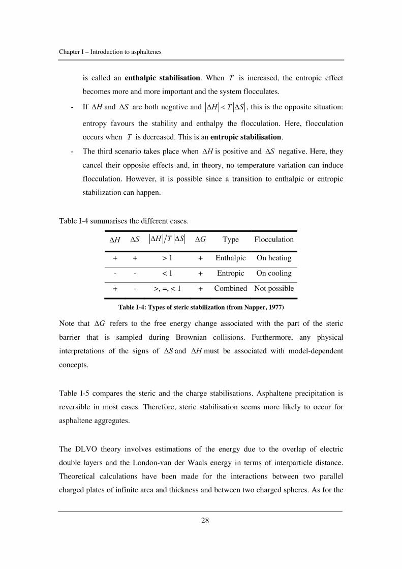
Table I-4 summarises the different cases.
HΔ SΔ H T SΔ Δ GΔ Type Flocculation
+ + > 1 + Enthalpic On heating
- - < 1 + Entropic On cooling
+ - >, =, < 1 + Combined Not possible
Table I-4: Types of steric stabilization (from Napper, 1977)
Note that GΔ refers to the free energy change associated with the part of the steric
barrier that is sampled during Brownian collisions. Furthermore, any physical
interpretations of the signs of SΔ and HΔ must be associated with model-dependent
concepts.
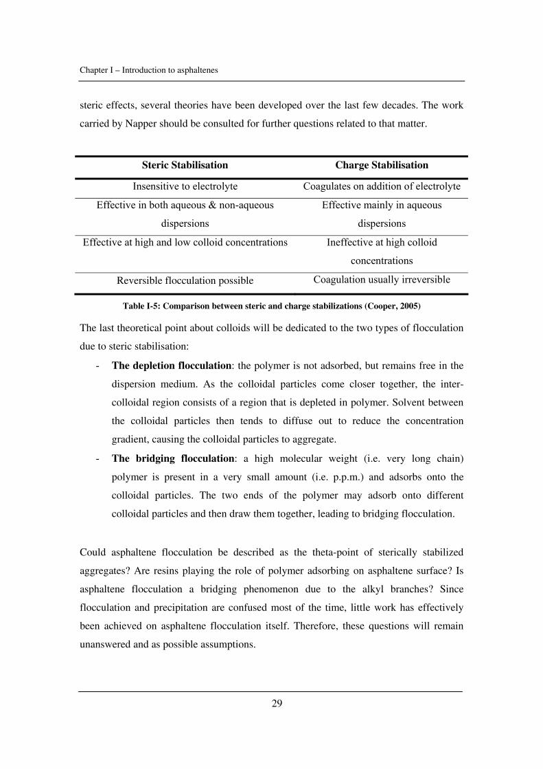
Table I-5 compares the steric and the charge stabilisations. Asphaltene precipitation is
reversible in most cases. Therefore, steric stabilisation seems more likely to occur for
asphaltene aggregates.
The DLVO theory involves estimations of the energy due to the overlap of electric
double layers and the London-van der Waals energy in terms of interparticle distance.
Theoretical calculations have been made for the interactions between two parallel
charged plates of infinite area and thickness and between two charged spheres. As for the
Chapter I – Introduction to asphaltenes
29
steric effects, several theories have been developed over the last few decades. The work
carried by Napper should be consulted for further questions related to that matter.
Steric Stabilisation Charge Stabilisation
Insensitive to electrolyte Coagulates on addition of electrolyte
Effective in both aqueous & non-aqueous
dispersions
Effective mainly in aqueous
dispersions
Effective at high and low colloid concentrations Ineffective at high colloid
concentrations
Reversible flocculation possible Coagulation usually irreversible
Table I-5: Comparison between steric and charge stabilizations (Cooper, 2005)
The last theoretical point about colloids will be dedicated to the two types of flocculation
due to steric stabilisation:
- The depletion flocculation: the polymer is not adsorbed, but remains free in the
dispersion medium. As the colloidal particles come closer together, the inter-
colloidal region consists of a region that is depleted in polymer. Solvent between
the colloidal particles then tends to diffuse out to reduce the concentration
gradient, causing the colloidal particles to aggregate.
- The bridging flocculation: a high molecular weight (i.e. very long chain)
polymer is present in a very small amount (i.e. p.p.m.) and adsorbs onto the
colloidal particles. The two ends of the polymer may adsorb onto different
colloidal particles and then draw them together, leading to bridging flocculation.
Could asphaltene flocculation be described as the theta-point of sterically stabilized
aggregates? Are resins playing the role of polymer adsorbing on asphaltene surface? Is
asphaltene flocculation a bridging phenomenon due to the alkyl branches? Since
flocculation and precipitation are confused most of the time, little work has effectively
been achieved on asphaltene flocculation itself. Therefore, these questions will remain
unanswered and as possible assumptions.
Chapter I – Introduction to asphaltenes
30
2.3.2. Asphaltene precipitation and flocculation
First, the difference between precipitation and flocculation shall be detailed: when a
precipitant is added (or when a pressure or temperature modification destabilises the
system), asphaltene aggregates start agglomerating: this is the flocculation. Then, when
gravity forces can overcome Brownian forces - when particles are larger than
1 mμ (Ferworn et al., 1993) - agglomerates can settle out of solution, this is the
asphaltene precipitation.
Let us briefly investigate this competition between diffusion (Brownian forces) and
sedimentation forces (gravity and buoyancy), which is expressed by the Péclet number:
Gravity induced motion LvPeBrownian motion D
−= = Eq I - 1
where L , v and D are respectively the characteristic length, velocity and diffusivity of
the particle.
The terminal velocity is attained when the driving force on the particle and the resistance
of the liquid are equal:
1 liquidparticle
particle
m g fvρρ
⎛ ⎞− =⎜ ⎟⎜ ⎟
⎝ ⎠ Eq I - 2
where m is the mass, ρ the density, g the local acceleration due to gravity and f the
frictional coefficient of the particle in the given medium.
Thus the Péclet number is:
1 liquidparticle
particle
agPe mDf
ρρ
⎛ ⎞= −⎜ ⎟⎜ ⎟
⎝ ⎠ Eq I - 3
where a is the diameter of the particle (which is assumed to be spherical).
According to the Einstein’s law of diffusion, the diffusion coefficient of a suspended
material at rest (i.e. no turbulence) in a steady state is related to the frictional coefficient
as follows:
Df kT= Eq I - 4
where k is the Boltzman’s constant and T the temperature.
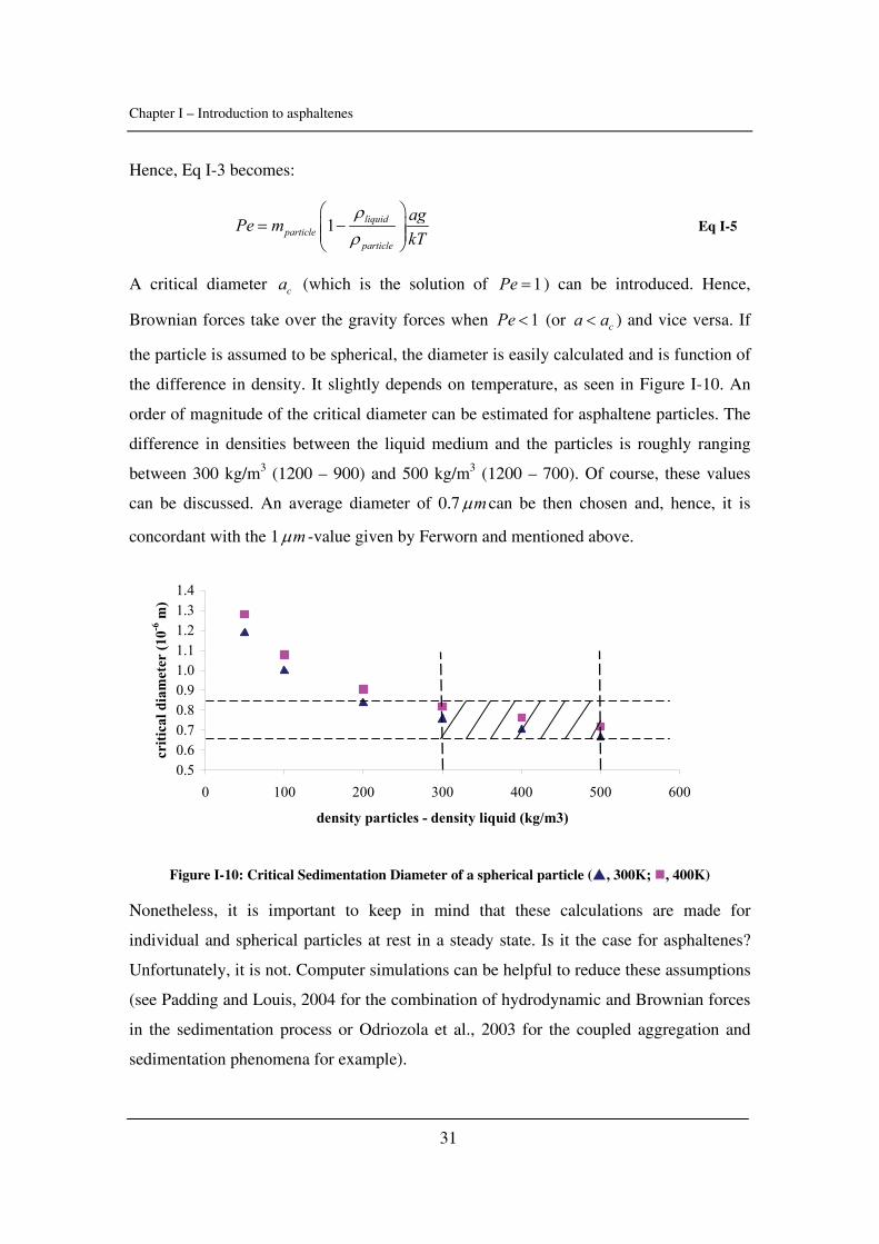
Chapter I – Introduction to asphaltenes
31
Hence, Eq I-3 becomes:
1 liquidparticle
particle
agPe mkT
ρρ
⎛ ⎞= −⎜ ⎟⎜ ⎟
⎝ ⎠ Eq I-5
A critical diameter ca (which is the solution of 1Pe = ) can be introduced. Hence,
Brownian forces take over the gravity forces when 1Pe < (or ca a< ) and vice versa. If
the particle is assumed to be spherical, the diameter is easily calculated and is function of
the difference in density. It slightly depends on temperature, as seen in Figure I-10. An
order of magnitude of the critical diameter can be estimated for asphaltene particles. The
difference in densities between the liquid medium and the particles is roughly ranging
between 300 kg/m3 (1200 – 900) and 500 kg/m3 (1200 – 700). Of course, these values
can be discussed. An average diameter of 0.7 mμ can be then chosen and, hence, it is
concordant with the 1 mμ -value given by Ferworn and mentioned above.
0.50.60.70.80.91.01.11.21.31.4
0 100 200 300 400 500 600
density particles - density liquid (kg/m3)
criti
cal d
iam
eter
(10-6
m)
Figure I-10: Critical Sedimentation Diameter of a spherical particle ( , 300K; , 400K)
Nonetheless, it is important to keep in mind that these calculations are made for
individual and spherical particles at rest in a steady state. Is it the case for asphaltenes?
Unfortunately, it is not. Computer simulations can be helpful to reduce these assumptions
(see Padding and Louis, 2004 for the combination of hydrodynamic and Brownian forces
in the sedimentation process or Odriozola et al., 2003 for the coupled aggregation and
sedimentation phenomena for example).
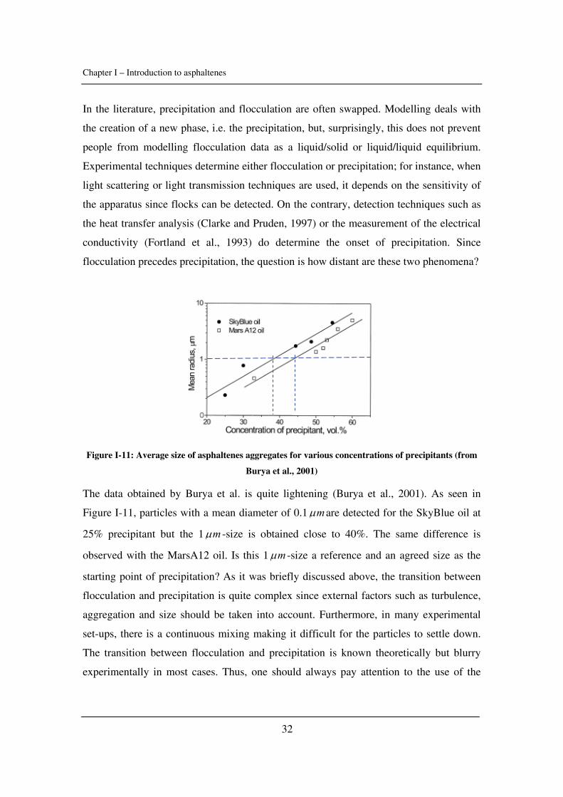
Chapter I – Introduction to asphaltenes
32
In the literature, precipitation and flocculation are often swapped. Modelling deals with
the creation of a new phase, i.e. the precipitation, but, surprisingly, this does not prevent
people from modelling flocculation data as a liquid/solid or liquid/liquid equilibrium.
Experimental techniques determine either flocculation or precipitation; for instance, when
light scattering or light transmission techniques are used, it depends on the sensitivity of
the apparatus since flocks can be detected. On the contrary, detection techniques such as
the heat transfer analysis (Clarke and Pruden, 1997) or the measurement of the electrical
conductivity (Fortland et al., 1993) do determine the onset of precipitation. Since
flocculation precedes precipitation, the question is how distant are these two phenomena?
Figure I-11: Average size of asphaltenes aggregates for various concentrations of precipitants (from
Burya et al., 2001)
The data obtained by Burya et al. is quite lightening (Burya et al., 2001). As seen in
Figure I-11, particles with a mean diameter of 0.1 mμ are detected for the SkyBlue oil at
25% precipitant but the 1 mμ -size is obtained close to 40%. The same difference is
observed with the MarsA12 oil. Is this 1 mμ -size a reference and an agreed size as the
starting point of precipitation? As it was briefly discussed above, the transition between
flocculation and precipitation is quite complex since external factors such as turbulence,
aggregation and size should be taken into account. Furthermore, in many experimental
set-ups, there is a continuous mixing making it difficult for the particles to settle down.
The transition between flocculation and precipitation is known theoretically but blurry
experimentally in most cases. Thus, one should always pay attention to the use of the
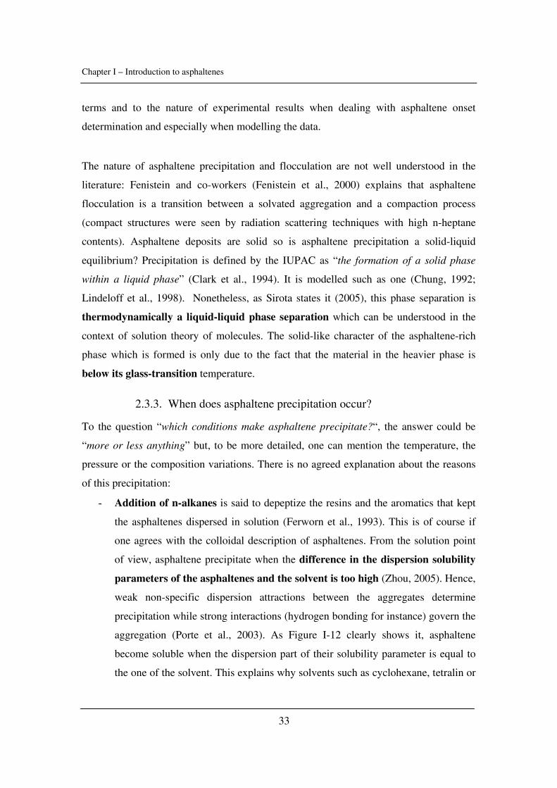
Chapter I – Introduction to asphaltenes
33
terms and to the nature of experimental results when dealing with asphaltene onset
determination and especially when modelling the data.
The nature of asphaltene precipitation and flocculation are not well understood in the
literature: Fenistein and co-workers (Fenistein et al., 2000) explains that asphaltene
flocculation is a transition between a solvated aggregation and a compaction process
(compact structures were seen by radiation scattering techniques with high n-heptane
contents). Asphaltene deposits are solid so is asphaltene precipitation a solid-liquid
equilibrium? Precipitation is defined by the IUPAC as “the formation of a solid phase
within a liquid phase” (Clark et al., 1994). It is modelled such as one (Chung, 1992;
Lindeloff et al., 1998). Nonetheless, as Sirota states it (2005), this phase separation is
thermodynamically a liquid-liquid phase separation which can be understood in the
context of solution theory of molecules. The solid-like character of the asphaltene-rich
phase which is formed is only due to the fact that the material in the heavier phase is
below its glass-transition temperature.
2.3.3. When does asphaltene precipitation occur?
To the question “which conditions make asphaltene precipitate?“, the answer could be
“more or less anything” but, to be more detailed, one can mention the temperature, the
pressure or the composition variations. There is no agreed explanation about the reasons
of this precipitation:
- Addition of n-alkanes is said to depeptize the resins and the aromatics that kept
the asphaltenes dispersed in solution (Ferworn et al., 1993). This is of course if
one agrees with the colloidal description of asphaltenes. From the solution point
of view, asphaltene precipitate when the difference in the dispersion solubility
parameters of the asphaltenes and the solvent is too high (Zhou, 2005). Hence,
weak non-specific dispersion attractions between the aggregates determine
precipitation while strong interactions (hydrogen bonding for instance) govern the
aggregation (Porte et al., 2003). As Figure I-12 clearly shows it, asphaltene
become soluble when the dispersion part of their solubility parameter is equal to
the one of the solvent. This explains why solvents such as cyclohexane, tetralin or
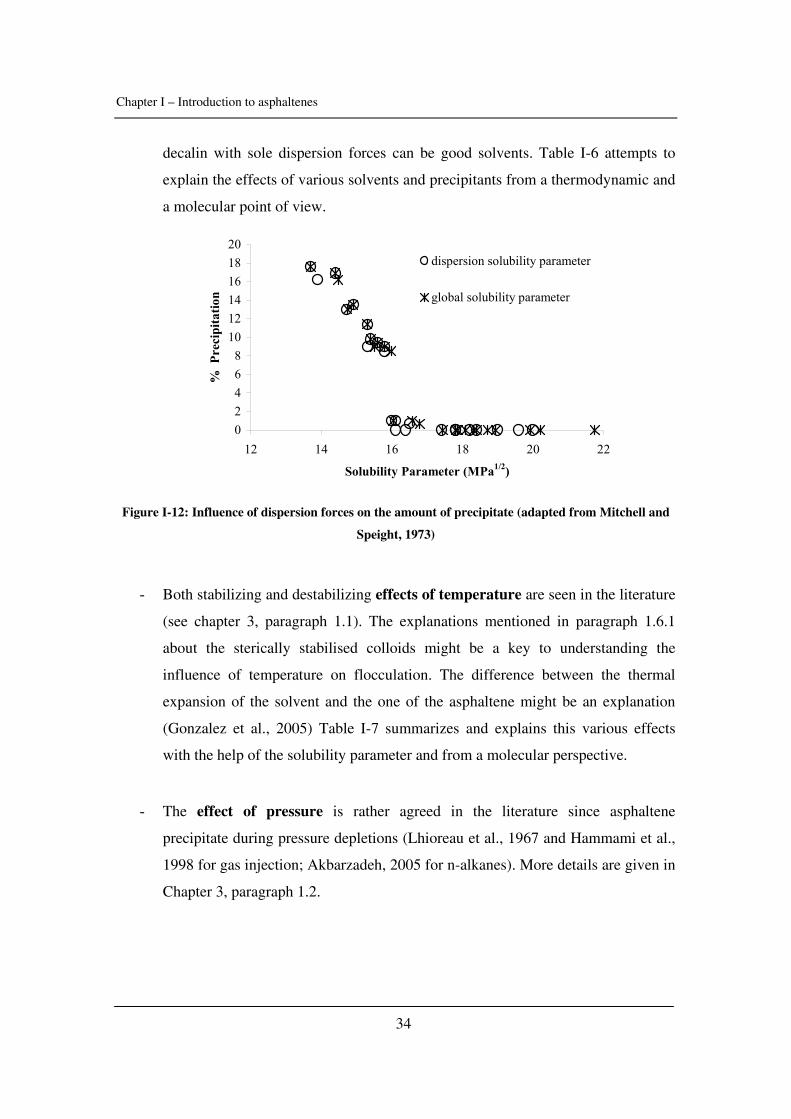
Chapter I – Introduction to asphaltenes
34
decalin with sole dispersion forces can be good solvents. Table I-6 attempts to
explain the effects of various solvents and precipitants from a thermodynamic and
a molecular point of view.
02468
101214161820
12 14 16 18 20 22
Solubility Parameter (MPa1/2)
% P
reci
pita
tion
dispersion solubility parameter
global solubility parameter
Figure I-12: Influence of dispersion forces on the amount of precipitate (adapted from Mitchell and
Speight, 1973)
- Both stabilizing and destabilizing effects of temperature are seen in the literature
(see chapter 3, paragraph 1.1). The explanations mentioned in paragraph 1.6.1
about the sterically stabilised colloids might be a key to understanding the
influence of temperature on flocculation. The difference between the thermal
expansion of the solvent and the one of the asphaltene might be an explanation
(Gonzalez et al., 2005) Table I-7 summarizes and explains this various effects
with the help of the solubility parameter and from a molecular perspective.
- The effect of pressure is rather agreed in the literature since asphaltene
precipitate during pressure depletions (Lhioreau et al., 1967 and Hammami et al.,
1998 for gas injection; Akbarzadeh, 2005 for n-alkanes). More details are given in
Chapter 3, paragraph 1.2.
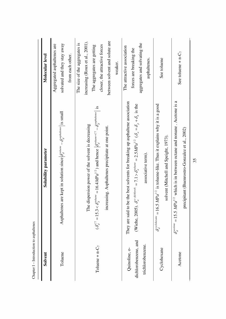
Cha
pter
I –
Int
rodu
ctio
n to
asp
halte
nes
35
Solv
ent
Solu
bilit
y pa
ram
eter
M
olec
ular
leve
l
Tol
uene
A
spha
lten
es a
re k
ept i
n so
luti
on s
ince
tolu
ene
asph
alte
nes
dd
δδ
−is
sm
all
Agg
rega
ted
asph
alte
nes
are
solv
ated
and
they
sta
y aw
ay
from
eac
h ot
her.
Tol
uene
+ n
-C7
The
dis
pers
ion
pow
er o
f th
e so
lven
t is
decr
easi
ng
(7
1/2
15.3
16.4
Cto
luen
ed
dM
Paδ
δ=
<=
) an
d he
nce
7to
luen
eC
asph
alte
nes
dd
δδ
+−
is
incr
easi
ng. A
spha
lten
es p
reci
pita
te a
t one
poi
nt.
The
siz
e of
the
aggr
egat
es is
incr
easi
ng (
Rou
x et
al.,
200
1).
The
agg
rega
tes
are
gett
ing
clos
er, t
he a
ttra
ctiv
e fo
rces
betw
een
solv
ent a
nd s
olut
e ar
e
wea
ker.
Qui
noli
ne, o
-
dich
loro
benz
ene,
and
tric
hlor
oben
zene
.
The
y ar
e sa
id to
be
the
best
sol
vent
s fo
r br
eaki
ng u
p as
phal
tene
ass
ocia
tion
(Wie
he, 2
005)
. .
1/2
7.1
2.5
odi
chlo
rob
tolu
ene
aa
MPa
δδ
−=
>=
(a
ph
δδ
δ=
+ is
the
asso
ciat
ive
term
).
The
att
ract
ive
asso
ciat
ion
forc
es a
re b
reak
ing
the
aggr
egat
es a
nd s
olva
ting
the
asph
alte
nes.
Cyc
lohe
xane
1/
216
.5cy
cloh
exan
ed
MPa
δ=
is to
luen
e-lik
e. T
hus
it ex
plai
ns w
hy it
is a
goo
d
solv
ent (
Mitc
hell
and
Spe
ight
, 197
3).
See
tolu
ene
Ace
tone
1/
215
.5ac
eton
ed
MPa
δ=
whi
ch is
in b
etw
een
octa
ne a
nd n
onan
e . A
ceto
ne is
a
prec
ipit
ant (
Bue
nros
tro-
Gon
zale
z et
al.,
200
2)
See
tolu
ene
+ n
-C7

Cha
pter
I –
Int
rodu
ctio
n to
asp
halte
nes
36
Met
hano
l 1/
215
.1m
etha
nol
dM
Paδ
= is
in b
etw
een
hexa
ne a
nd h
epta
ne. M
etha
nol i
s a
prec
ipit
ant (
And
erse
n, 1
997)
. Se
e to
luen
e +
n-C
7
Nit
roge
n
2N dδ
is b
etw
een
1 an
d 4
1/2
MPa
(bet
wee
n 1
and
50 M
Pa a
nd 2
93 a
nd 3
83 K
).
The
dis
pers
ion
pow
er o
f th
e so
lven
t is
high
ly d
ecre
ased
. Pre
cipi
tati
on m
ay
occu
r de
pend
ing
on th
e m
isci
bili
ty o
f 2
N in
the
solv
ent.
Nit
roge
n is
wea
keni
ng th
e
attr
acti
ve f
orce
s so
lven
t-so
lute
.
Hen
ce, t
he a
ggre
gate
s at
trac
t
each
oth
er, a
ggre
gate
and
floc
cula
te.
2C
O
2C
O h
as o
nly
disp
ersi
on a
nd q
uadr
upol
ar f
orce
s bu
t the
qua
drup
olar
are
assu
med
not
to h
ave
spec
ific
infl
uenc
e he
re.
2C
Odδ
is v
aryi
ng b
etw
een
3 an
d
16
1/2
MPa
(be
twee
n 1
and
50 M
Pa a
nd 2
93 a
nd 3
83 K
). T
hese
str
ong
vari
atio
ns a
ffec
t the
sol
ubil
ity p
aram
eter
of
the
solv
ent v
ery
muc
h,
espe
cial
ly s
ince
2
CO
is v
ery
solu
ble.
Idem
as
nitr
ogen
Tab
le I
-6:
Infl
uenc
e of
the
sol
vent
on
the
stab
ility
of
asph
alte
nes
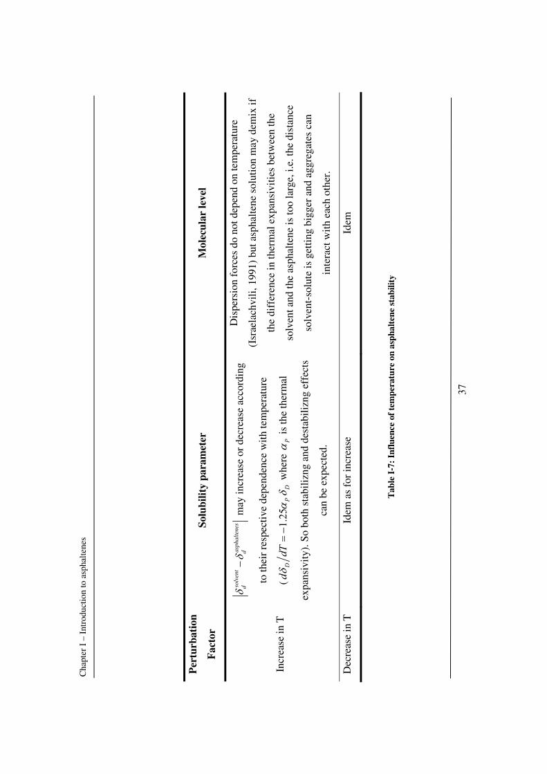
Cha
pter
I –
Int
rodu
ctio
n to
asp
halte
nes
37
Per
turb
atio
n
Fac
tor
Solu
bilit
y pa
ram
eter
M
olec
ular
leve
l
Incr
ease
in T
solv
ent
asph
alte
nes
dd
δδ
− m
ay in
crea
se o
r de
crea
se a
ccor
ding
to th
eir
resp
ecti
ve d
epen
denc
e w
ith
tem
pera
ture
(1.
25D
PD
ddT
δα
δ=−
whe
re
Pα
is th
e th
erm
al
expa
nsiv
ity)
. So
both
sta
bili
zng
and
dest
abili
zng
effe
cts
can
be e
xpec
ted.
Dis
pers
ion
forc
es d
o no
t dep
end
on te
mpe
ratu
re
(Isr
aela
chvi
li, 1
991)
but
asp
halt
ene
solu
tion
may
dem
ix if
the
diff
eren
ce in
ther
mal
exp
ansi
viti
es b
etw
een
the
solv
ent a
nd th
e as
phal
tene
is to
o la
rge,
i.e.
the
dist
ance
solv
ent-
solu
te is
get
ting
big
ger
and
aggr
egat
es c
an
inte
ract
wit
h ea
ch o
ther
.
Dec
reas
e in
T
Idem
as
for
incr
ease
Id
em
Tab
le I
-7:
Infl
uenc
e of
tem
pera
ture
on
asph
alte
ne s
tabi
lity
Chapter I – Introduction to asphaltenes
38
Almost all the possible techniques have been used to detect asphaltene precipitation:
microscopic examination, optical transmission and light-scattering, conductivity
measurements, viscosimetry, particle size analysis, fluorescence spectroscopy, density
measurements or acoustic methods (see Andersen, 1999 for the different references or
Chapter 3, paragraph 2). Every technique brings useful information:
- The work done by Jill Buckley with refractive index (Buckley, 1999) shows that
precipitation is strongly linked to van der Waals forces. The refractive index
only takes into account dispersion forces (Israelachvili, 1991). It corroborates
what has been said previously.
- Onset titrations (Cimino et al., 1995) showed that, surprisingly, the onset of
precipitation of asphaltene solutions does not depend on the asphaltene
concentration but only on the solvent quality. This might suggest- that
asphaltene fugacity does not depend on its molar fraction. This last piece of
information does not have so much physical sense but it should be remembered if
modelling is attempted.
- By means of SANS measurements and varying the n-heptane content in a toluene
solution of asphaltenes, it was seen the aggregate size is increasing but the
small-scale internal structure is unchanged (Roux et al., 2001). In the same
paper, it was concluded that asphaltene precipitation is similar under temperature
or composition variations, although the amplitudes and kinetics might be
different. Experiments at the onset were tried but unfortunately they were not
reproducible or stable. This emphasizes the need of more information about the
onset of precipitation.
So, asphaltene precipitation and flocculation are distinct phenomena linked to the size of
aggregates, the turbulence. It is difficult to detect the transition between these two
phenomena from an experimental point of view, especially if the solution is mixed and
particles cannot settle down. Flocculation is related to the colloidal nature of asphaltenes
and both steric and charge stabilisations are at stake. Precipitation is a liquid-liquid
transition from a thermodynamic point of view and it is linked to the dispersion forces of
the solvent and the asphaltenes.
Chapter I – Introduction to asphaltenes
39
2.3.4. The reversibility
This is again a controversial issue, even in recent papers though the asphaltene
community tends to agree now that asphaltene precipitation is reversible (Porte et al.,
2003). Two schools of thought are in opposition; one considers that asphaltenes are
dissolved in the oil in a true liquid state and that they may precipitate depending on the
thermodynamic conditions. The second one states that asphaltenes are solid particles
dispersed in the crude oil and stabilised by large resin molecules. Asphaltene flocculation
and precipitation would be irreversible. Both views are based on experimental
observations but it is believed in this work that precipitation is reversible.
When pressure is smaller than the lower pressure onset or higher than the upper pressure
onset, asphaltenes are likely to go back to solution. As Hammami suggested it (2000),
asphaltene precipitation is generally reversible but the kinetics of redissolution vary
significantly depending on the physical state of the system. Some authors claim that the
asphaltene composition has a key role in the reversibility issue (Leontaristis, 1994).
Nonetheless, it is not clearly explained or proved. It was also stated that asphaltene
precipitation is less likely to be reversible for crude oils subjected to conditions well
beyond those of the precipitation onset (Fotland, 1996).
The hysteresis between asphaltene precipitation and redissolution has been studied
(Andersen, 1992; Peramanu et al., 2001; Hammami et al., 2000). This hysteresis can be
due the precipitation factor (composition, temperature or pressure). The hysteresis with
temperature (Peramanu et al., 2001) seems more important than with pressure (Hammami
et al., 2000). Since different oils were studied, it seems hazardous to conclude. The
hysteresis may also be linked to deposition. Actually, if asphaltenes are deposited, their
re-dissolution will take much longer. It is interesting to note that complete reversibility
could be obtained after sonication (Mohamed et al., 1999).
Chapter I – Introduction to asphaltenes
40
2.4. Unanswered questions
Several points will be shortly introduced in this paragraph but will not be developed:
- Asphaltenes are mainly studied in solvent solutions and not in crude oils (neutron
scattering, determination properties, study of interactions). But what is the
validity of such measurements?
- Kinetics has a major impact on the study of phase behaviour and stability but little
attention is paid to this factor. Can the results found in the literature be trusted? Is
the equilibrium reached in the fields when asphaltene precipitate?
- Deposition is the problematic issue. Asphaltenes may precipitate but not deposit if
the flowrate is sufficient for instance. There are very few studies about this topic.
Should the efforts not be directed in this way?
Chapter I – Introduction to asphaltenes
41
3. Asphaltenes and Petroleum industry
The technical issues surrounding asphaltenes are complex, first of all because their
understanding, their definition, their structures, to name a few of the problems, are partly
confusing and still subject to harsh debates amongst “experts”. Then, it is often when
fluids have very little asphaltenes that they are problematic. Finally, asphaltenes create
troubles from the production of the oil to the refinery process.
In this paragraph, the various problems encountered by the oil industry will be evocated
with a special focus on gas injection. Then, the solutions used to treat and handle
asphaltene problems will be briefly described.
3.1. The problems related to asphaltenes in the oil industry
The main problems caused by asphaltenes can be divided in several groups (Pineda-
Flores et al., 2001):
- The extraction: when asphaltenes precipitate and deposit, they are likely to clock
the porous space, hence reducing the permeability and the crude’s exit flux. It
does also affect the wettability (Cuiec, 1984). Iwere and co-workers (Iwere et al.,
2002) modelled the effects of asphaltene precipitation on fluid flow and oil
production from the fractured reservoirs of the Taratunich Field. The effects of
asphaltene precipitation were modelled through changes in pore volume and
transmissibility with reservoir pressure. The analysis of the reservoir and well
performance data revealed that lithology and pore throat size played an important
role in determining where asphaltene precipitates in the reservoirs. Abdulrazag
and Shedid investigated the effect of fracture characteristics on reduction of
permeability by asphaltene deposition in carbonate formation. They studied the
influence of the flow rate and the stress, among other things (Abdulrazag and
Shedid, 2004). Some simulations were also tried coupled with a thermodynamic
model (Nghiem et al., 2000; Monteagudo et al., 2002). Although the results are
claimed to be in agreement with experimental results, thermodynamic models are
known to behave poorly when dealing with asphaltenes.
Chapter I – Introduction to asphaltenes
42
- Transport: blending incompatible oils that can lead to asphaltene precipitation is
a well-known issue in the oil industry. Wiehe dedicated many articles to this
topic. He based his work and predictions on solubility parameters. Titrations at
atmospheric conditions can help finding the right proportions (Wiehe and
Kennedy, 2004).
- Processing: Catalyst deactivation is the main problem. When hydrotreating heavy
oils, both the non-asphaltenic phase and the asphaltenes undergo a chemical
conversion, which may lead to unstable products as well as to increased coke lay-
down on the catalyst (Bartholdi and Andersen, 2000). Fouling in heat-exchangers
is also a major issue (Dickakian and Seay, 1988).
- Crude exploitation: economical profits related to crude exploitation depend on
its chemical composition in such a way that crude with a high content of
asphaltenes (18-22%) is considered as “heavy” and low quality product. Since this
represents major difficulties in its extraction and refining, economical profit
notably diminishes.
- Environment: by collecting the oil-water interface of surface equipment, such as
free water knock outs and heater treaters, asphaltenes contribute to the formation
of stable emulsions that make oil-water separation difficult. This contaminated
water may pose problems (Stephenson, 1990).
3.2. A few words about the Enhanced Oil Recovery (EOR)
This paragraph is adapted from Morel and Roy, 2004. The term Enhanced Oil Recovery,
or EOR, was first used in the 1970s and reached the height of its popularity in the 1980s.
EOR methods are typically classified into three main categories:
- Thermal: This category covers steam injection and in-situ combustion which
designates injection of air, sometimes oxygen-enriched, in viscous oils where
oil/oxygen chemical reactions release large quantities of heat. These methods all
cause a temperature rise in the reservoir which considerably decreases the
viscosity of the oil in place.
- Gas injection: Not all types of gas injection are classified as EOR, and the
definitions are not always precise. The following are clearly classified as EOR:
Chapter I – Introduction to asphaltenes
43
o all injections of non-hydrocarbon gas (nitrogen, 2CO , 2H S , air…)
o injections of miscible or partially miscible hydrocarbon gas in the oil zone
o injections of hydrocarbon gas in zones already swept by water (this is
called tertiary recovery)
o alternating gas-water injections (Water Alternate Gas), whatever the gas
may be.
- Chemical: Chemical methods are classified in two major families. On the one
hand, injection of polymers can, enhance the macroscopic sweep efficiency of
water in viscous oil (more favourable mobility ratio) by increasing the viscosity of
the injection water. On the other hand, the injection of surfactants or alkaline
products enhances the microscopic sweep efficiency of water.
The following points are worth mentioning:
- EOR production represents only (about) 4% of overall worldwide production,
which is still very low. A slight increase has emerged in the past few years.
- Thermal methods are the most often used in the EOR category, covering around
2/3 of world EOR production. Gas injection follows with 25-30%, and the
remainder goes to chemical EOR methods which are still quite low.
- The leading country in terms of EOR is clearly the USA.
These classifications and statistics should evolve perceptibly in the years to come, with
the emergence of Mexico and its massive injection of nitrogen in the giant field of Akal
(in the Cantarell complex), helping increase production by about one million barrels per
day. It is also expected that Canada and Venezuela, which contain most of the world’s
heavy oil in place and are beginning to produce it, increase their production strongly
using thermal processes.
3.3. The Vapex Process
Solvent-based processes for recovery of heavy oil have attracted increasing attention in
the past few years as compared to steam-based processes, they may reduce the energy
consumption and greenhouse gas emission. The Vapour Extraction (VAPEX) process
was proposed by Butler and Mokrys for the first time in 1991 as an alternative to Steam
Chapter I – Introduction to asphaltenes
44
Assisted Gravity Drainage (SAGD) for thin reservoirs (Butler and Mokrys, 1991). The
VAPEX process is closely related to the SAGD concept where the steam chamber is
replaced with a chamber containing light hydrocarbon vapours close to its dew point at
the reservoir pressure. The heavy oil has its viscosity reduced by dissolution of the
injected solvent and is subsequently produced by a gravity drainage mechanism. Between
the pure VAPEX process (cold solvent injection) and the pure SAGD process, several
hybrid processes exist which combine the advantages of these two methods (Dauba et al.,
2002).
Propane and ethane are considered to be the most suitable solvents for the process.
However, a mixture of butane, propane and ethane can also be used, depending on the
prevailing pressure in the reservoir. One can wonder what will happen in terms of
asphaltene precipitation. One single study dealing with this question was found (Das and
Butler, 1994). This investigation was carried out in a Hele-Shaw cell using propane and
several heavy crudes. It was concluded that asphaltene deposition does not prevent the
flow of oil through the reservoir for the proposed production scheme. They also observed
that deasphalting takes place if the injected propane pressure is close to or higher than the
vapour pressure of propane at the same temperature. However, porosity is likely to be
affected by asphaltene precipitation and deposition. Asphaltene precipitation can also be
seen as an in-situ upgrading of the oil and it may help producing higher quality oils. The
main inconvenient of this process are the slow mixing bitumen/solvent as well as the
solvent losses, its supply, storage, compression and treatment before recycling.
3.4. CO2 injection
One of the problems of the VAPEX is the value of the hydrocarbon solvent, which is
partly lost in the reservoir. For this reason other cheaper solvents may be also envisaged,
particularly 2CO . Two cases are possible:
- Miscible CO2-EOR: the gas aims at decreasing the viscosity and, hence, at
recovering more oil. It happens in specific conditions (roughly, API>22 and depth
larger than 1200 m).
- Immiscible CO2-EOR: the gas is only used to re-pressurize the reservoir and to
push the oil towards the well.
Chapter I – Introduction to asphaltenes
45
2CO EOR is a current forefront topic in the domain of sustainable development as it
combines both enhanced recovery of hydrocarbons and geological storage of greenhouse
gases. Another important reason for EOR development is the commitment of all the
industry majors to reduce their greenhouse gas emissions. 2CO is a highly effective
enhanced recovery agent for some types of oil and we are presently witnessing the
multiplication of 2CO projects combining enhanced recovery operations and geological
storage of 2CO (Morel and Roy, 2004).
Currently, 20,000 tons per day of CO2 are delivered to oil fields for EOR projects
(Moritis 1998). A significant fraction of the injected 2CO remains in the reservoir, but
some is produced along with the oil. Generally, this 2CO is separated from the oil,
recompressed, and injected back into the reservoir. Total production is a little less than
200,000 bbl/day (3.2 x10⁴ m3/day) and thus roughly 10 bbl of oil are produced for
every ton of CO2 injected. Most of the 2CO for EOR originates from naturally occurring
geologic traps, although a small fraction is from anthropogenic sources (Stevens and
Gale, 2000). To date, 2CO injection projects have focused on oil with densities between
29 and 48 °API (855 to 711 kg/m3, respectively) and reservoir depths from 760 to 3700
m (Taber et al., 1997). Within the U.S., 2CO -EOR operations are centered in the Permian
and Rocky Mountain basins (Texas, New Mexico, and Colorado). Current use of 2CO for
oil recovery is limited by cost and availability of 2CO . If substantial additional quantities
of 2CO are made available due to sequestration efforts, significant 2CO storage capacity
remains to be exploited in oil reservoirs. Screening criteria have been proposed elsewhere
for selecting reservoirs where 2CO may sustain or increase the production of oil (Taber et
al., 1997). They estimate that upwards of 80% of oil reservoirs worldwide might be
suitable for CO2 injection based upon oil-recovery criteria alone. Moreover, the
process is widely applicable in both sandstone and carbonate formations with a variety of
permeabilities and thickness of hydrocarbon bearing zones. The major factors limiting
Chapter I – Introduction to asphaltenes
46
2CO injection as an oil recovery process have been availability of CO2 and the cost to
build pipelines to carry 2CO into oil producing regions (Jessen et al., 2005).
The effect of 2CO injection on asphaltene stability has been experienced in fields. Sarma
reports several cases in with serious asphaltene deposition due to 2CO flood: Midale
(Canada), Little Creek Field (Missisipi) and West Texas (Sarma, 2003). Laboratory and
simulations studies have also been carried on. In Chapter 3, paragraph 3.3, various papers
studying the influence of 2CO on asphaltene precipitation are listed.
3.5. Which oils/fields are problematic?
Field and laboratory data confirm that the lighter the oil, the lower is the asphaltene
solubility. Asphaltenes tend to precipitate more easily in light oils rather than in heavy
oils. For instance, the Venezuelan Boscan crude with 17.2 wt% asphaltene was produced
with nearly no troubles whereas Hassi-Messaoud in Algeria has numerous production
problems with only 0.15 wt% (Sarma, 2003). Since light-oil reservoirs are more often
candidates to gas injection processes, the danger is even bigger.
3.6. What are the solutions so far?
3.6.1. Prevention
Chemical treatment is often the prevention method used: dispersing agents are often
injected (60-70 ppm minimum at the bottom of the well). These dispersing agents are
often anionic/cationic mixtures. These asphaltene inhibitors are usually prepared in the
lab, by bottle tests. Since different asphaltene inhibitors work on different oils, all the
possible chemistries have to be tested to select the proper additive.
An adapted management of the oilfield – by keeping the pressure constant or preventing a
brutal depletion – will also avoid asphaltene precipitation, especially near the well-bore.
Furthermore, incompatible oils should not be mixed.
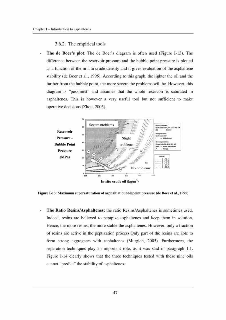
Chapter I – Introduction to asphaltenes
47
3.6.2. The empirical tools
- The de Boer’s plot: The de Boer’s diagram is often used (Figure I-13). The
difference between the reservoir pressure and the bubble point pressure is plotted
as a function of the in-situ crude density and it gives evaluation of the asphaltene
stability (de Boer et al., 1995). According to this graph, the lighter the oil and the
farther from the bubble point, the more severe the problems will be. However, this
diagram is “pessimist” and assumes that the whole reservoir is saturated in
asphaltenes. This is however a very useful tool but not sufficient to make
operative decisions (Zhou, 2005).
Figure I-13: Maximum supersaturation of asphalt at bubblepoint pressure (de Boer et al., 1995)
- The Ratio Resins/Asphaltenes: the ratio Resins/Asphaltenes is sometimes used.
Indeed, resins are believed to peptpize asphaltenes and keep them in solution.
Hence, the more resins, the more stable the asphaltenes. However, only a fraction
of resins are active in the peptization process.Only part of the resins are able to
form strong aggregates with asphaltenes (Murgich, 2005). Furthermore, the
separation techniques play an important role, as it was said in paragraph 1.1.
Figure I-14 clearly shows that the three techniques tested with these nine oils
cannot “predict” the stability of asphaltenes.
Severe problems
No problems
Slight
problems
In-situ crude oil (kg/m3)
Reservoir
Pressure –
Bubble Point
Pressure
(MPa)
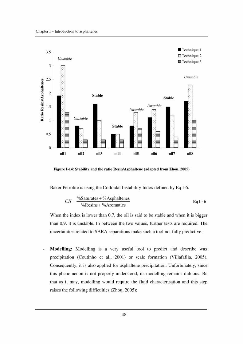
Chapter I – Introduction to asphaltenes
48
0
0.5
1
1.5
2
2.5
3
3.5
oil1 oil2 oil3 oil4 oil5 oil6 oil7 oil8
Rat
io R
esin
s/A
spha
lten
es
Technique 1
Technique 2
Technique 3
Stable
Unstable
UnstableUnstable
Unstable
Unstable
Stable
Stable
Figure I-14: Stability and the ratio Resin/Asphaltene (adapted from Zhou, 2005)
Baker Petrolite is using the Colloidal Instability Index defined by Eq I-6.
%Saturates %Asphaltenes%Resins %Aromatics
CII +=
+ Eq I - 6
When the index is lower than 0.7, the oil is said to be stable and when it is bigger
than 0.9, it is unstable. In between the two values, further tests are required. The
uncertainties related to SARA separations make such a tool not fully predictive.
- Modelling: Modelling is a very useful tool to predict and describe wax
precipitation (Coutinho et al., 2001) or scale formation (Villafafila, 2005).
Consequently, it is also applied for asphaltene precipitation. Unfortunately, since
this phenomenon is not properly understood, its modelling remains dubious. Be
that as it may, modelling would require the fluid characterisation and this step
raises the following difficulties (Zhou, 2005):
Chapter I – Introduction to asphaltenes
49
- Complex analytical methods are required in order to characterise asphaltenes
(C20+ fractions, SARA, asphaltenes molecular weight, polarity etc.).
- In addition, a special (and expensive) sampling method is necessary.
- Once the sample is available, the validity of experimental tests depends on the
flocculation detection limit at reservoir conditions and on the kinetics.
This issue is discussed in more details in Chapter 5.
3.6.3. Remediation
Common approaches to the asphaltene deposition problems can be summarized as
follows (Stephenson, 1990):
- Physical cleaning and removal: bailing, drilling or hydroblasting may be
necessary when asphaltenes collect in or plug the well bore. In oil field storage
tanks, precipitated asphaltenes must often be shoveled out of tank bottoms. These
operations are tedious and time consuming, the necessary equipment is expensive
and disposal of large volumes of washings can pose an environmental problem.
- Solvent treatment: although they show only slight activity, solvents such as
xylene can be used to disperse/dissolve asphaltenes. This approach is often
expensive due to the large dosages of solvent required. The environmental
concerns over low-molecular weight aromatic solvents also must be considered
- Treatment with low-molecular weight dispersants: dispersant treatment is
subject to the same types of difficulties as solvent treatment. Low molecular
weight dispersants such as cresylic acid, have an associated toxicity which makes
them less desirable to use
- Increased emulsion breaker concentration: asphaltenes can collect at the oil-
water interface, and some have been treated with high concentrations of emulsion
breakers. Sometimes this approach is effective probably due to the presence of a
minor emulsion breaker component with dispersancy activity. However, excess
treatment with demuslfiers is expensive.
The cost of such operations is obviously non-negligible. For instance, the shutdown and
the clean-up cost for a 8-inch submarine crude pipeline was estimated around 2.5 million
dollars in 1996 (Leontaritis, 1996).
Chapter I – Introduction to asphaltenes
50
4. Conclusion
This paragraph aimed at summarizing the main issues dealing with asphaltenes.
Obviously, much more could be said and discussed, for both theoretical and industrial
point of view. The goal was only to emphasize the complex nature of asphaltenes in order
to enlighten the other parts of this thesis.
The main theoretical points about asphaltenes presented in this chapter were:
- Asphaltenes are the most polar and heavier part of petroleum. Their mere
definition is still a subject of debate amongst experts. The technique used to
extract them strongly influences their nature.
- Asphaltenes can be easily characterized in terms of solubility parameters.
- Asphaltene molecules are either from the archipelago or the continental type.
- Asphaltenes have a double nature: colloids and solutes in a solvent. Flocculation
and precipitation are directly linked to this double nature.
- The molecular weight of asphaltene monomers is around 1000 g/mol
- Self-association starts around 100 ppm. It is mainly due to hydrogen bonding.
- Dispersion forces (and polar forces to a less extent) govern the asphaltene
precipitation.
- The CMC about asphaltenes (if any) is not due to the sole asphaltene structure.
- Resins have a co-solubilizing effect on asphaltenes.
- Flocculation is a state of aggregation that precedes precipitation (which is a phase
transition). Flocculation is ruled by colloidal stability whereas precipitation can be
explained in terms of solubility parameters.
- Asphaltene precipitation is reversible in most cases. It is likely to be governed by
kinetics.
Chapter I – Introduction to asphaltenes
51
5. Aim of this project
This project has several objectives dealing with asphaltene stability related to gas
injection:
- Developing experimental methods to determine input parameters for the models,
especially solubility parameters of crude oils and asphaltenes and critical
constants of asphaltenes. The effect of pressure is of particular interest.
- Studying the influence of gas injection on asphaltene stability and the eventual
effects of temperature and pressure.
- Investigating asphaltene precipitation by means of calorimetry for live oils, dead
oils and asphaltene solutions.
- Test models based on cubic EOS and evaluate a new model taking aggregation
into account.
Chapter I – Introduction to asphaltenes
52
Literature
Abdulrazag Y. Z., Shedid A. S., The effect of fracture characteristics on reduction of permeability by asphaltene precipitation in carbonate formation, J. Pet. Sci. Eng. (2004), 42, 171– 182 Akbarzadeh K., Alboudwarej H., Svrcek W., Yarranton H.W., A generalized regular solution model for asphaltene precipitation from n-alkane diluted heavy oils and bitumen, Fluid Phase Equilibr. (2005), 232, 159 - 170 Al-Sahhaf T.A., Fahim M.A., Elkilani A.S., Retardation of asphaltene precipitation by addition of toluene, resins, deasphalted oil and surfactants, Fluid Phase Equilibr. (2002), 194 – 197, 1047 - 1057 Andersen S.I., Hysteresis in precipitation and dissolution of petroleum asphaltenes, Fuel Sci. Technol. Intl. (1992), 10, 1743 - 1749 Andersen S.I., Concentration effects in HPLC-SEC analysis of petroleum asphaltenes, J. Liq. Chromatogr. (1994), 17, 4065-4079 Andersen S.I., Separation of asphaltenes by polarity using liquid-liquid extraction, Pet. Sci. Technol. (1997), 15, 185-198 Andersen S.I., Flocculation onset titration of petroleum asphaltenes, Energ. Fuel. (1999), 13, 315 – 322 Andersen S.I., Birdi K.S., Aggregation of asphaltenes as determined by calorimetry, J. Colloid. Interf. Sci. (1991), 142, 497-502 Andersen S.I., Birdi K.S., Influence of temperature and solvent on the precipitation of asphaltenes, Fuel Sci. Techn. Int. (1990), 8, 593 – 615 Andersen S.I., Hofsäss T., Kleintiz W., Rahimian I., Organic precipitates in oil production of a Venezuelan oil field, Pet. Sci. Technol. (2001 a), 19, 55- 74 Andersen S.I., del Rio J.M., Khvostitchenko D., Shakir S., Lira-Galeana C., Interaction and solubilization of water by petroleum asphaltenes in organic solution, Langmuir (2001 b), 17, 307-313 Andersen, S.I., Speight J.G., Petroleum resins: separation, character, and role in petroleum, Pet. Sci. Technol. (2001), 19, 1 – 34
Chapter I – Introduction to asphaltenes
53
Andersen S.I., Vigild M., Effect of chemical alteration on the aggregation of asphaltenes in d-toluene using SANS, Proceedings of The 6th International Conference on Petroleum Phase Behaviour and Fouling, Amsterdam, 2005 Andersen S.I., Jensen O., Speight J.G., X-ray Diffraction of Subfractions of Petroleum Asphaltenes, Energ. Fuel. (2005), 19, 2371 – 2377 Andreatta G., Bostrom N., Mullins O.C., High-Q ultrasonic determination of the critical nanoaggregate concentration of asphaltenes and the critical micelle concentration of standards surfactants, Langmuir (2005), 21, 2728 – 2736 Aquino-Olivos M.A., Andersen S.I., Lira-Galeana C., Comparisons between asphaltenes from the dead and live-oil samples of the same crude oils, Pet. Sci. Technol. (2003), 21, 1017-1041 Bartholdy J., Andersen S.I., Changes in asphaltene stability during hydrotreating, Energ. Fuel. (2000), 14, 52-55 Bissada K. K., Szymczyk E. B., Nolte D.G., Darnell L. M., Improved asphaltene and paraffin separations and quantification for crude oil and bitumen characterization, Presented at 6th International Conference on Petroleum Phase Behaviour and Fouling, Amsterdam, June 2005 de Boer R.B., Leerloyer K., Eigner M.R.P., van Bergen A.R.D., Screening of crude oils for asphalt precipitation: theory, practice, and the selection of inhibitors, SPE Prod. Facil. (1995), 55 – 61 Buckley J.S., Predicting the onset of asphaltene precipitation from refractive index measurements, Energ. Fuel. (1999), 13, 328 – 332 Buenrostro-Gonzalez E., Andersen S.I., Garcia-Martinez J.A., Lira-Galeana C., Solubility/molecular structure relationships of asphaltenes in polar and non-polar media, Energ. Fuel. (2002), 16, 732 – 741 Burya Y.G., Yudin I.K., Dechabo V.A., Anisimov M.A., Colloidal properties of crude oils studied by dynamic light-scattering, Int. J. Thermophys. (2001), 22, 5, 1397 – 1410 Butler, R.M., Mokrys, I.J., A new process (VAPEX) for recovering heavy oils using hot water and hydrocarbon vapour”, J.C.P.T. (Jan. 1991), 97 Carbognani L., Solid petroleum asphaltenes seem surrounded by alkyl layers, Pet. Sci. Technol. (2003), 21, 537-556 Castillo J., Hung J., Fernandez A., Mujica V., Nonlinear optical evidences of aggregation in asphaltene-toluene solutions, Fuel (2001), 80, 1239 - 1243
Chapter I – Introduction to asphaltenes
54
Chung F.T.H., Thermodynamic modelling for organic solid precipitation, SPE 24851 (1992), 869 – 878 Cimino R., Correra S., Del Bianco A., Lockart T.P., Solubility and Phase Behaviour of asphaltenes in hydrocarbon media, Asphaltenes: Fundamentals and Applications, Sheu E.Y., Mullins O.C., Ed., Plenum Press, NY, 97 - 130 (1995) Clark J.B., Hastie J.W., Kihlborg L.H.E., Metselaar R., Thackeray M.M., Definitions of terms relating to phase transitions of the solid state, Pure & App. Chem. (1994), 66, 577-594 Clarke P.F., Pruden B.P, Asphaltene precipitation: detection using heat transfer analysis, and inhibition using chemical additives, Fuel (1997), 76, 7, 607 – 614 Cooper S., Course Notes, Department of Chemistry, University of Durham, England (http://www.dur.ac.uk/sharon.cooper/lectures/colloids/interfacesweb1.html), 2005 Coutinho J.A.P., Pauly J., Daridon J.L., A thermodynamic model to predict wax formation in petroleum fluids, Braz. J. Chem. Eng. (2001), 18, 411 - 422 Cuiec L., Rock/crude oil interactions and weattbility: an attempt to understand their interaction, Proceedings of SPE Annual Technical Conference and Exhibition (1984), Das S.K., Butler R. M., Effect of Asphaltene Deposition on the Vapex Process: A Preliminary Investigation Using a Hele-Shaw Cell, J. Can. Petrol. Technol. (1994), 33, 39-45 Dauba C., Quettier L., Christensen J., Le Goff C., Cordelier P., An Integrated Experimental and Numerical Approach to Assess the Performance of Solvent Injection into Heavy Oil, Proceedings - SPE Annual Technical Conference and Exhibition (2002), 1131-1140 Diallo M.S., Cagin T., Faulon J.L, Goddard III W.A., Thermodynamic properties of asphaltenes: a predictive approach base don computer assisted structure elucidation and atomistic simulations, in “Asphaltene and asphalts, 2. Developments in Petroleum Science, 40 B”, Edited by T.F. Yen and G.V. Chilingarian, chap. 5, 2000 Dickakian G., Seay S., Asphaltene precipitation primary crude exchanger fouling mechanism, Oil Gas J. (1988), 86, 47-50 Dickie J.P., Yen T.F., Anal. Chem. (1967), 39, 1847 Eilers H., The colloidal structure of asphalt, J. Phy. Chem. (1949), 53, 1195 – 1211
Chapter I – Introduction to asphaltenes
55
Fenistein D., Barré L., Frot D., Oil Gas Sci. Technol. (2000), 55, 123 – 128 Ferworn K.A., Svrcek W.Y., Mehortra A.K., Measurement of asphaltene particle size distribution in crude oils diluted with n-heptane, Ind. Eng. Chem. Res. (1993), 32, 955 – 959 Fotland P., Precipitation of asphaltenes at high-pressures; Experimental technique and results, Fuel Sci. Techn. Int. (1996), 14, 313 - 325 Fotland P., Anfindsen H., Fadnes F.H., Detection of asphaltene precipitation and amounts precipitated by measurement of electrical conductivity, Fluid Phase Equilibr. (1993), 82, 157 – 164 Hammami A., Ferworn K.A:, Nighswander J.A., Overå S., Stange E., Asphaltenic crude oil characterization: an experimental investigation of the effect of resins on the stability of asphaltenes, Pet. Sci. Technol. (1998), 16, 227 – 249 Hammami A., Phelps C.H., Monger-McClure T., Little T.M., Asphaltene precipitation from live oils: an experimental investigation of onset conditions and reversibility, Energ. Fuel. (2000), 14, 14 – 18 Hotier G., Robin M., Action de divers diluants sur les produits pétroliers lourds : mesure, interprétation et prévision de la floculation des asphaltenes, Rev. I. Fr. Petrol. (1983), 38, 1, 101 – 120 Israelachvili J., Intermolecular and surface forces, 2nd edition, Academic Press, London, 1991 Iwere, F.O., Apaydin, O.G., Moreno, J.E., Simulation of asphaltene precipitation in fractured reservoirs: a case study, SPE 74373, SPE International Petroleum Conference and Exhibition, Mexico, Villahermosa, Mexico, 10– 12 February 2002 Jessen K., Kovscek A.R., Orr F.M. Jr., Increasing 2CO storage in oil recovery, Energ.
Conve. .Manag. (2005), 46, 293–311 Klein G.C., Yen A., Asomaning S., Rodgers R.P., Marshall A.G., High resolution mass spectrometry compositional comparison of the heptane precipitated asphaltenes and asphaltenes induced from reduction of pressure, Proceedings of the 6th International Conference on Petroleum Phase Behaviour and Fouling, Amsterdam, June 2005 Kontogeorgis G., Intermolecular Forces & Hydrogen Bonding, Course Notes, Department of Chemical Engineering, Technical University of Denmark, 2005
Chapter I – Introduction to asphaltenes
56
Leontaritis K.J., Amaefule J.O., Charles R.E., A systematic approach for the prevention of formation damage caused by asphaltene precipitation, SPE Prod. Facil. (1994), 9, 157-164 Leontaritis K.J., Offshore asphaltene and wax deposition: problems/solutions, World Oil (1996), 217, 57-63 Lhioreau C., Briant J., Tindy R., Influence de la pression sur la floculation des asphaltenes, Rev. I. Fr. Petrol. (1967), 22, 797 - 806 Lindeloff N., Heidemann R.A., Andersen S.I., Stenby E.H., A thermodynamic mixed-solid asphaltene precipitation model, Pet. Sci. Technol. (1998), 16, 3&4, 307 - 321 Maruska H.P., Rao B.M.L., The role of polar species in the aggregation of asphaltenes, Fuel. Sci. Tech. Int. (1987), 5, 119 - 168 Merino-Garcia D., Calorimetric investigations of asphaltene self-association and interaction with resins, Ph.D. Thesis, IVC-SEP, Department of Chemical Engineering, Denmark, Technical University, Lyngby, Denmark, 2003 Merino-Garcia D., Andersen S.I., Calorimetric evidence about the application of the concept of CMC to asphaltene self-association, J. Dispers. Sci. Technol. (2005), 26, 217-225 Mitchell D.L., Speight J.G., The solubility of asphaltenes in hydrocarbon solvents, Fuel (1973), 52, 149 – 152 Mohamed R.S., Loh W., Ramos A.C.S., Delgado C.C., Almeida V.R., Reversibility and inhibition of asphaltene in Brazilian crude oils, Pet. Sci. Technol. (1999), 17, 877 – 896 Monteagudo J.E.P., Rajagopal K., Lage, P.L.C., Simulating oil flow in porous media under asphaltene deposition, Chem. Eng. Sci. (2002), 57, 323-337 Morel D., Roy C., EOR: high-potential technologies for mature fields, Technoscoop (2004), 28, 34 – 41 Moritis, G., 1998 Worldwide EOR Survey, Oil Gas J. (Apr. 1998), 20, 49-97 Moschopedis S.E., Speight J.G., Hydrogen bonding by oxygen functions in Athabasca bitumen, Fuel (1976), 55, 187 - 192 Müller-Dethlefs K., Hobza K., Noncovalent interactions: a challenge for experiment and theory, Chem. Rev. (2000), 100, 143 – 167
Chapter I – Introduction to asphaltenes
57
Murgich J., Intermolecular forces in aggregates of asphaltenes and resins, Pet. Sc. Technol. (2002), 20, 983 - 997 Murgich J., Molecular mechanics study of the selectivity in the interaction between some typical resins and asphaltenes, Proceedings of the 6th International Conference on Petroleum Phase Behaviour and Fouling, Amsterdam, June 2005 Nagel R.G., Hunter B.E., Peggs J.K., Fong D.K., Mazzocchi E., Tertiary application of a hydrocarbon miscible flood. Rainbow Keg River ‘B’ pool, SPE Reservoir Eng. (1990), 5, 301-308 Napper D.H., Steric stabilization, J. Colloid. Interf. Sci. (1977), 58, 390 - 407 Nghiem L.X., Kohse B.F., Ali S.M.F., Doan Q., Asphaltene precipitation: Phase behaviour modelling and compositional simulation, Proceedings of the SPE Asia Pacific Conference on Integrated Modelling for Asset Management, 283-296, 2000 Odriozola G., Leone R., Schmitt A., Moncho-Jorda A., Hidalgo-Alvarez R., Coupled aggregation and sedimentation processes: the sticking probability effect, Phys. Rev. E. (2003) 67, 031401, 1-5 Padding J.T., Louis A. A., Hydrodynamic and brownian fluctuations in sedimenting suspensions, Phys. Rev. Letters (2004), 93, 220601, 1-4 Pedersen C., Asphaltene characterization: permittivity measurements and modelling, Ph.D. Thesis, IVC-SEP, Department of Chemical Engineering, Denmark, Technical University, Lyngby, Denmark, 2000 Peramanu S., Singh C., Agrawala M., Yarranton H.W., Investigation on the reversibility of asphaltene precipitation, Energ. Fuel. (2001), 15, 910 – 917 Pineda-Flores G., Mesta-Howard A.M., Petroleum asphaltenes: generated problematic and possible biodegradation mechanism, Rev. Lat. Microbiologia (2001), 43, 3, 143 – 150 Porte G., Zhou H., Lazzeri V., Reversible description of asphaltene colloidal association and precipitation, Langmuir (2003), 19, 40 – 47 Prausnitz J.M., Lichtenthaler R.N., Gomes de Azevedo E., Molecular thermodynamics of Fluid-Phase Equilibria (3rd edition), Prentice Hall PTR, New Jersey, 1999 Ravey J.C., Ducouret G., Espinat D., Asphaltene macrostructure by small-angle neutron-scattering, Fuel (1988), 67, 1560 - 1567
Chapter I – Introduction to asphaltenes
58
Rogacheva O.V., Rimaev R.N., Gubaidullin V.Z., Khazimov D.K., Investigation of the surface activity of the asphaltenes of petroleum residues, Colloid J. USSR (1980), 42, 586 - 589 Rogel E., Theoretical estimation of the solubility parameter distributions of asphaltenes, Energ. Fuel (1997), 11, 920-925 Rogel E., Carbognani L., Density estimation of asphaltenes using molecular dynamic simulations, Energ. Fuel. (2003), 17, 378 – 386 Rogel E., Leon O., Torres G., Espidel J., Aggregation of asphaltenes in organic solvents using surface tension measurements, Fuel (2000), 79, 1389- 1394 Roux J.N., Brosseta D., Demé B., SANS study of asphaltene aggregation: concentration and solvent quality effects, Langmuir (2001), 17, 5085 - 5092 Sallamie N., Shaw J.M., Heat capacity prediction for polynuclear aromatic solids using vibration spectra, Fluid Phase Equilb. (2005), 237, 100 – 110 Speight J.G., Moschopedis S.E., On the molecular nature of petroleum asphaltenes, Adv. Chem. Ser. (1981), 195, 1 – 15 Sarma H.K., Can we ignore asphaltene in a gas injection project for light oils?, Proceedings - SPE International Improved Oil Recovery Conference in Asia Pacific (2003), 193-199 Shaw D.J., Introduction to colloid and surface chemistry, 4th edition, Butterworth-Heinemann Publications, Oxford, 1992 Sheu E.Y., Mullins O.C., Asphaltenes: Fundamentals and Applications, Ed., Plenum Press, NY (1995) Sheu E.Y., De Tar M.M., Storm D.A., Dielectric properties of asphaltene solutions, Fuel (1994), 73, 1, 45 - 50 Siffert B., Kuczinski J., Papirer E., Relationship between electrical charge and flocculation of heavy oil distillation residues in organic medium, J. Coll. Int. Sci. (1990), 135, 107 – 117 Sirota E.B., Physical structure of asphaltenes, Energ. Fuel. (2005), 19, 1290-1296 Speight J.G., Plancher H., Molecular models for petroluemasphaltenes and implications for asphalt science and technology, Proc. Int. Symp. On Chemistry of Bitumens (1991), 154
Chapter I – Introduction to asphaltenes
59
Speight, J.G., The Chemistry and Technology of Petroleum, 3rd ed., Marcel Dekker, NY (1999) Speight J.G., Chemical and Physical studies of petroleum asphaltenes, in Asphaltenes and asphalts, 1. Developments in petroleum science, 40, Ed. by Yen T.F., Chilingrian G.V., Elsevier Science, Amsterdam, 7 – 65 (1994), Stephenson W.K., Producing asphaltenic crude oils: problems and solutions, Petrol. Eng. Int. (1990), 24 - 91 Stevens S.H., Gale, J., Geologic 2CO Sequestration May Benefit Upstream Industry, Oil
Gas J. (2000), 15, 40-44 Sztukowski D.M., Jafari, J., Alboudwarej H., Yarranton H.W., Asphaltene self-association and water-in-hydrocarbon emulsions, J. Colloid. Interf. Sci. (2003), 265, 179–186 Taber J.J., Martin F. D., Seright R.S., EOR Screening Criteria Revisited—Part 1: Introduction to Screening Criteria and Enhanced Recovery Field Projects, Soc. Pet. Eng. Res. Eng. (1997), 189-198 Tissot B.P., Welste D.H., Petroleum formation and occurrence, Second Edition, Ed. Springer-Verlag, Berlin, 1984 Villafafila A., Measurement and Modelling of Scaling Minerals, PhD Thesis, Department of Chemical Engineering, Technical University of Denmark, 2005 Wiehe I.A., In Defense of Vapor Pressure Osmometry for Measuring Molecular Weight, Proceedings of the 6th International Conference on Petroleum Phase Behaviour and Fouling, Amsterdam, June 2005 Wiehe I.A., Kennedy R.J., Oil compatibility model and crude oil incompatibility, Energ. Fuel. (2000), 14, 56-59 Yarranton H.W., Issues in characterizing asphaltenes and other heavy fraction components, Proceedings of the 6th International Conference on Petroleum Phase Behaviour and Fouling, Amsterdam, June 2005 Yen T.F., Asphaltenes: types and sources, in “Structures and Dynamics of Asphaltenes”, Ed. by Mullins O.C., Sheu E.Y., Plenum Press, NY (1995), 1 - 20 Yen T.F., Chilingrian G.V., Asphaltenes and asphalts, 1. Developments in petroleum science, 40, Elsevier Science, Amsterdam (1994)

Chapter I – Introduction to asphaltenes
60
Zhou H., Total Research Centre, Pau, France, Personal communication (2005) Websites: The asphaltene standardization discussion: http://asphaltenes.syncrude-research.karo.com/users/folder.asp
Chapter II – Characterization of Crude Oils and Asphaltenes
61
Chapter II
Characterization of Crude Oils and
Asphaltenes
Chapter II – Characterization of Crude Oils and Asphaltenes
62
Table of Contents
1. Introduction............................................................................................................. 65
1.1. A brief overview about characterization of crude oil ....................................... 65
1.2. Solubility parameter: definition and determination .......................................... 69
1.2.1. Definition .................................................................................................. 69
1.2.2. Determination and measurement .............................................................. 72
1.3. Influence of pressure and temperature.............................................................. 74
1.3.1. Solubility parameter from PR EOS........................................................... 74
1.3.2. Influence of temperature ........................................................................... 74
1.3.3. Influence of pressure................................................................................. 77
1.3.4. Solubility parameters of gases .................................................................. 78
1.4. Conclusion ........................................................................................................ 79
2. Solubility parameter of crude oil........................................................................... 80
2.1. Internal pressure, an alternative ........................................................................ 80
2.2. Internal pressure of pure compounds................................................................ 84
2.3. Internal pressure of crude oils........................................................................... 86
2.4. Conclusion ........................................................................................................ 89
3. Characterization of asphaltenes ............................................................................ 90
3.1. Solubility parameter of asphaltenes .................................................................. 90
3.1.1. Literature survey ....................................................................................... 90
3.1.2. Partial volumes and regular solution theory ............................................. 93
3.1.3. Experimental procedure, calibration and results....................................... 95
3.1.4. Conclusion ................................................................................................ 97
3.2. Critical parameters of asphaltenes .................................................................... 98
3.2.1. Method based on partial volumes ............................................................. 98
Chapter II – Characterization of Crude Oils and Asphaltenes
63
3.2.2. Method based on NMR data ................................................................... 100
3.2.3. Comparison between the two methods ................................................... 103
4. Conclusion ............................................................................................................. 105
Literature....................................................................................................................... 106
List of symbols............................................................................................................... 111
Chapter II – Characterization of Crude Oils and Asphaltenes
64
Can solubility parameters or critical parameters of asphaltenes – widely employed to
model the phase behaviour of asphaltenic fluids – be measured? How trustful would such
measurements be? Can the effect of pressure and temperature be taken into account?
This chapter describes several techniques developed for crude oils and asphaltenes in
order to characterize them. First, a brief overview of oil characterization is given and is
followed by the definition of the solubility parameter and its various properties. Then, an
alternative approach using internal pressure to determine the solubility parameter of
crude oil is presented. Finally, solubility parameters and critical constants of asphaltenes
are determined with various techniques.
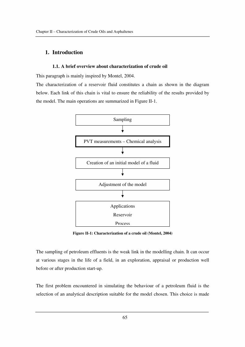
Chapter II – Characterization of Crude Oils and Asphaltenes
65
1. Introduction
1.1. A brief overview about characterization of crude oil
This paragraph is mainly inspired by Montel, 2004.
The characterization of a reservoir fluid constitutes a chain as shown in the diagram
below. Each link of this chain is vital to ensure the reliability of the results provided by
the model. The main operations are summarized in Figure II-1.
Figure II-1: Characterization of a crude oil (Montel, 2004)
The sampling of petroleum effluents is the weak link in the modelling chain. It can occur
at various stages in the life of a field, in an exploration, appraisal or production well
before or after production start-up.
The first problem encountered in simulating the behaviour of a petroleum fluid is the
selection of an analytical description suitable for the model chosen. This choice is made
Sampling
PVT measurements – Chemical analysis
Creation of an initial model of a fluid
Adjustment of the model
Applications
Reservoir
Process
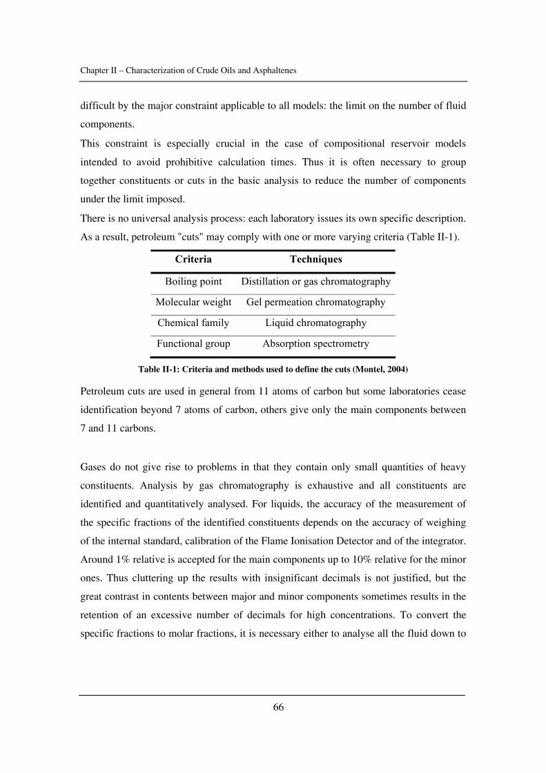
Chapter II – Characterization of Crude Oils and Asphaltenes
66
difficult by the major constraint applicable to all models: the limit on the number of fluid
components.
This constraint is especially crucial in the case of compositional reservoir models
intended to avoid prohibitive calculation times. Thus it is often necessary to group
together constituents or cuts in the basic analysis to reduce the number of components
under the limit imposed.
There is no universal analysis process: each laboratory issues its own specific description.
As a result, petroleum "cuts" may comply with one or more varying criteria (Table II-1).
Criteria Techniques
Boiling point Distillation or gas chromatography
Molecular weight Gel permeation chromatography
Chemical family Liquid chromatography
Functional group Absorption spectrometry
Table II-1: Criteria and methods used to define the cuts (Montel, 2004)
Petroleum cuts are used in general from 11 atoms of carbon but some laboratories cease
identification beyond 7 atoms of carbon, others give only the main components between
7 and 11 carbons.
Gases do not give rise to problems in that they contain only small quantities of heavy
constituents. Analysis by gas chromatography is exhaustive and all constituents are
identified and quantitatively analysed. For liquids, the accuracy of the measurement of
the specific fractions of the identified constituents depends on the accuracy of weighing
of the internal standard, calibration of the Flame Ionisation Detector and of the integrator.
Around 1% relative is accepted for the main components up to 10% relative for the minor
ones. Thus cluttering up the results with insignificant decimals is not justified, but the
great contrast in contents between major and minor components sometimes results in the
retention of an excessive number of decimals for high concentrations. To convert the
specific fractions to molar fractions, it is necessary either to analyse all the fluid down to
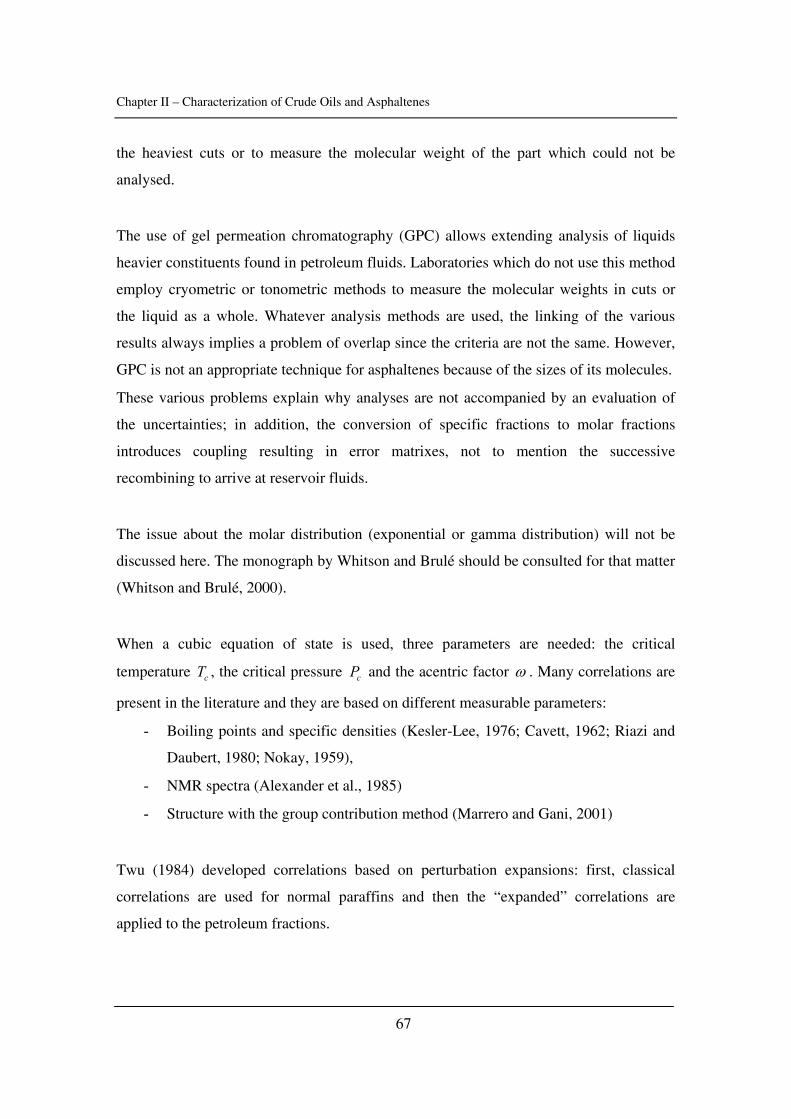
Chapter II – Characterization of Crude Oils and Asphaltenes
67
the heaviest cuts or to measure the molecular weight of the part which could not be
analysed.
The use of gel permeation chromatography (GPC) allows extending analysis of liquids
heavier constituents found in petroleum fluids. Laboratories which do not use this method
employ cryometric or tonometric methods to measure the molecular weights in cuts or
the liquid as a whole. Whatever analysis methods are used, the linking of the various
results always implies a problem of overlap since the criteria are not the same. However,
GPC is not an appropriate technique for asphaltenes because of the sizes of its molecules.
These various problems explain why analyses are not accompanied by an evaluation of
the uncertainties; in addition, the conversion of specific fractions to molar fractions
introduces coupling resulting in error matrixes, not to mention the successive
recombining to arrive at reservoir fluids.
The issue about the molar distribution (exponential or gamma distribution) will not be
discussed here. The monograph by Whitson and Brulé should be consulted for that matter
(Whitson and Brulé, 2000).
When a cubic equation of state is used, three parameters are needed: the critical
temperature cT , the critical pressure cP and the acentric factor ω . Many correlations are
present in the literature and they are based on different measurable parameters:
- Boiling points and specific densities (Kesler-Lee, 1976; Cavett, 1962; Riazi and
Daubert, 1980; Nokay, 1959),
- NMR spectra (Alexander et al., 1985)
- Structure with the group contribution method (Marrero and Gani, 2001)
Twu (1984) developed correlations based on perturbation expansions: first, classical
correlations are used for normal paraffins and then the “expanded” correlations are
applied to the petroleum fractions.
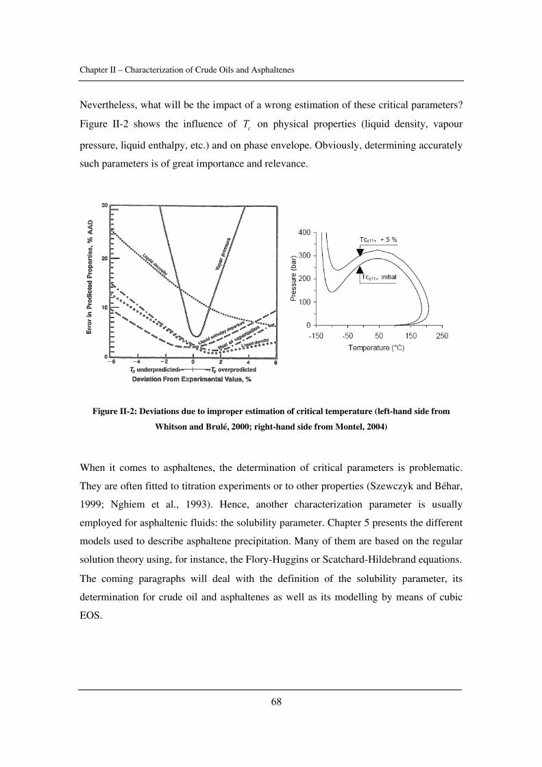
Chapter II – Characterization of Crude Oils and Asphaltenes
68
Nevertheless, what will be the impact of a wrong estimation of these critical parameters?
Figure II-2 shows the influence of cT on physical properties (liquid density, vapour
pressure, liquid enthalpy, etc.) and on phase envelope. Obviously, determining accurately
such parameters is of great importance and relevance.
Figure II-2: Deviations due to improper estimation of critical temperature (left-hand side from
Whitson and Brulé, 2000; right-hand side from Montel, 2004)
When it comes to asphaltenes, the determination of critical parameters is problematic.
They are often fitted to titration experiments or to other properties (Szewczyk and Béhar,
1999; Nghiem et al., 1993). Hence, another characterization parameter is usually
employed for asphaltenic fluids: the solubility parameter. Chapter 5 presents the different
models used to describe asphaltene precipitation. Many of them are based on the regular
solution theory using, for instance, the Flory-Huggins or Scatchard-Hildebrand equations.
The coming paragraphs will deal with the definition of the solubility parameter, its
determination for crude oil and asphaltenes as well as its modelling by means of cubic
EOS.
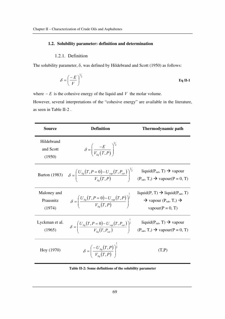
Chapter II – Characterization of Crude Oils and Asphaltenes
69
1.2. Solubility parameter: definition and determination
1.2.1. Definition
The solubility parameter, δ, was defined by Hildebrand and Scott (1950) as follows:
21
⎟⎠⎞
⎜⎝⎛ −
=VEδ Eq II-1
where E− is the cohesive energy of the liquid and V the molar volume.
However, several interpretations of the “cohesive energy” are available in the literature,
as seen in Table II-2 .
Source Definition Thermodynamic path
Hildebrand
and Scott
(1950) ( )
12
,liq
EV T P
δ⎛ ⎞−
= ⎜ ⎟⎜ ⎟⎝ ⎠
Barton (1983) ( ) ( )
( )2
1
,,0,
⎟⎟⎠
⎞⎜⎜⎝
⎛ −==
PTVPTUPTU
liq
satvapliqδ liquid(Psat, T) vapour
(Psat, T,) vapour(P = 0, T)
Maloney and
Prausnitz
(1974)
( ) ( )( )
21
,,0,
⎟⎟⎠
⎞⎜⎜⎝
⎛ −==
PTVPTUPTU
liq
vapliqδ
liquid(P, T) liquid(Psat, T)
vapour (Psat, T,)
vapour(P = 0, T)
Lyckman et al.
(1965)
( ) ( )( )
21
,,0,
⎟⎟⎠
⎞⎜⎜⎝
⎛ −==
satliq
satvapliq
PTVPTUPTU
δ liquid(Psat, T) vapour
(Psat, T,) vapour(P = 0, T)
Hoy (1970) ( )( )
21
,,
⎟⎟⎠
⎞⎜⎜⎝
⎛ −=
PTVPTU
liq
liqδ (T,P)
Table II-2: Some definitions of the solubility parameter
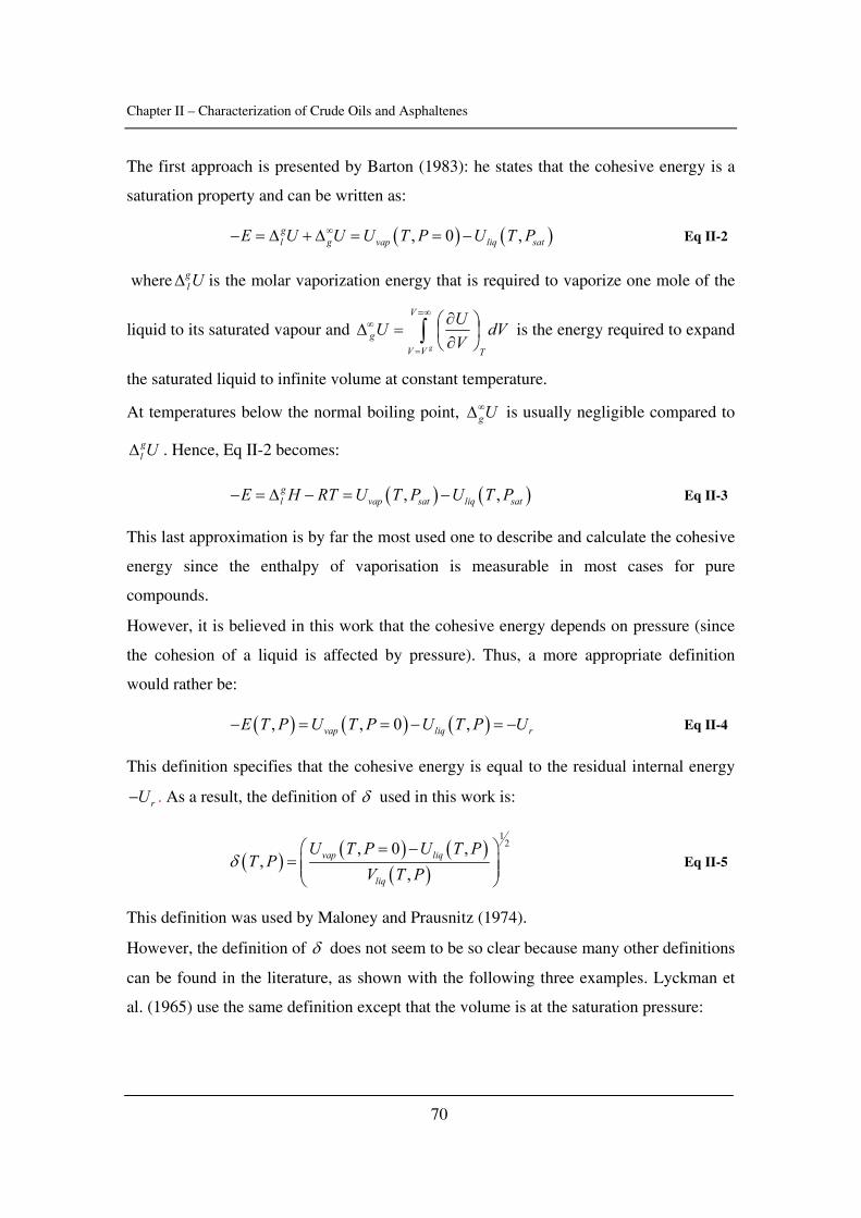
Chapter II – Characterization of Crude Oils and Asphaltenes
70
The first approach is presented by Barton (1983): he states that the cohesive energy is a
saturation property and can be written as:
( ) ( ), 0 ,gl g vap liq satE U U U T P U T P∞− = Δ + Δ = = − Eq II-2
where UglΔ is the molar vaporization energy that is required to vaporize one mole of the
liquid to its saturated vapour and dVVUU
T
V
VVg
g∫
∞=
=
∞ ⎟⎠⎞
⎜⎝⎛
∂∂
=Δ is the energy required to expand
the saturated liquid to infinite volume at constant temperature.
At temperatures below the normal boiling point, gU∞Δ is usually negligible compared to
gl UΔ . Hence, Eq II-2 becomes:
( ) ( ), ,gl vap sat liq satE H RT U T P U T P− = Δ − = − Eq II-3
This last approximation is by far the most used one to describe and calculate the cohesive
energy since the enthalpy of vaporisation is measurable in most cases for pure
compounds.
However, it is believed in this work that the cohesive energy depends on pressure (since
the cohesion of a liquid is affected by pressure). Thus, a more appropriate definition
would rather be:
( ) ( ) ( ), , 0 ,vap liq rE T P U T P U T P U− = = − = − Eq II-4
This definition specifies that the cohesive energy is equal to the residual internal energy
rU− . As a result, the definition of δ used in this work is:
( ) ( ) ( )( )
12, 0 ,
,,
vap liq
liq
U T P U T PT P
V T Pδ
⎛ ⎞= −= ⎜ ⎟⎜ ⎟
⎝ ⎠ Eq II-5
This definition was used by Maloney and Prausnitz (1974).
However, the definition of δ does not seem to be so clear because many other definitions
can be found in the literature, as shown with the following three examples. Lyckman et
al. (1965) use the same definition except that the volume is at the saturation pressure:
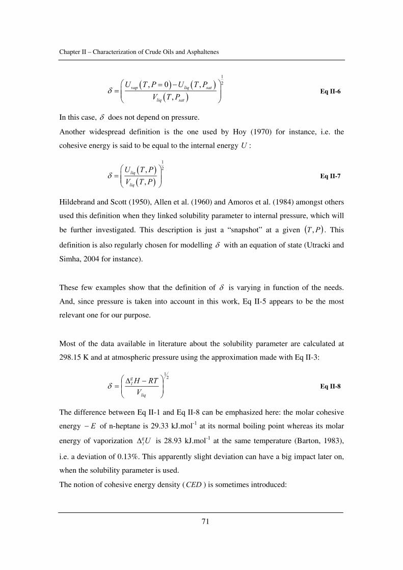
Chapter II – Characterization of Crude Oils and Asphaltenes
71
( ) ( )( )
12, 0 ,
,vap liq sat
liq sat
U T P U T PV T P
δ⎛ ⎞= −
= ⎜ ⎟⎜ ⎟⎝ ⎠
Eq II-6
In this case, δ does not depend on pressure.
Another widespread definition is the one used by Hoy (1970) for instance, i.e. the
cohesive energy is said to be equal to the internal energy U :
( )( )
12,
,liq
liq
U T PV T P
δ⎛ ⎞
= ⎜ ⎟⎜ ⎟⎝ ⎠
Eq II-7
Hildebrand and Scott (1950), Allen et al. (1960) and Amoros et al. (1984) amongst others
used this definition when they linked solubility parameter to internal pressure, which will
be further investigated. This description is just a “snapshot” at a given ( )PT , . This
definition is also regularly chosen for modelling δ with an equation of state (Utracki and
Simha, 2004 for instance).
These few examples show that the definition of δ is varying in function of the needs.
And, since pressure is taken into account in this work, Eq II-5 appears to be the most
relevant one for our purpose.
Most of the data available in literature about the solubility parameter are calculated at
298.15 K and at atmospheric pressure using the approximation made with Eq II-3:
21
⎟⎟⎠
⎞⎜⎜⎝
⎛ −Δ=
liq
gl
VRTH
δ Eq II-8
The difference between Eq II-1 and Eq II-8 can be emphasized here: the molar cohesive
energy E− of n-heptane is 29.33 kJ.mol-1 at its normal boiling point whereas its molar
energy of vaporization UglΔ is 28.93 kJ.mol-1 at the same temperature (Barton, 1983),
i.e. a deviation of 0.13%. This apparently slight deviation can have a big impact later on,
when the solubility parameter is used.
The notion of cohesive energy density (CED ) is sometimes introduced:
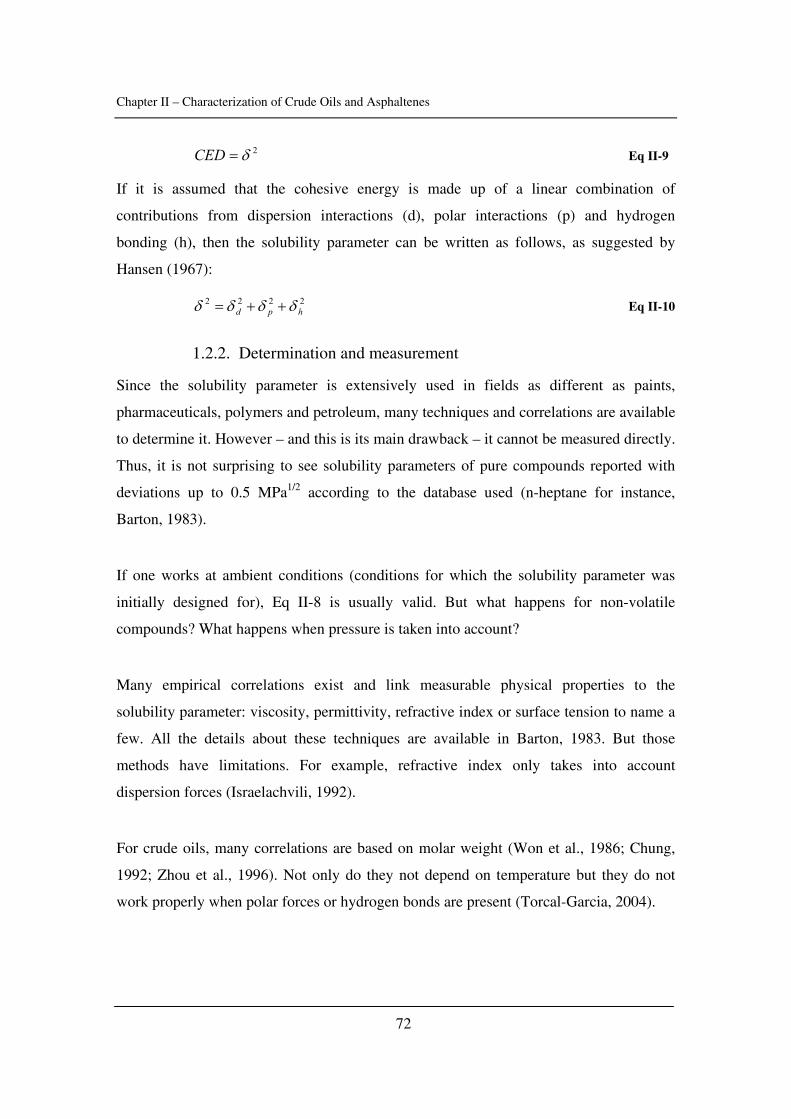
Chapter II – Characterization of Crude Oils and Asphaltenes
72
2δ=CED Eq II-9
If it is assumed that the cohesive energy is made up of a linear combination of
contributions from dispersion interactions (d), polar interactions (p) and hydrogen
bonding (h), then the solubility parameter can be written as follows, as suggested by
Hansen (1967):
2222hpd δδδδ ++= Eq II-10
1.2.2. Determination and measurement
Since the solubility parameter is extensively used in fields as different as paints,
pharmaceuticals, polymers and petroleum, many techniques and correlations are available
to determine it. However – and this is its main drawback – it cannot be measured directly.
Thus, it is not surprising to see solubility parameters of pure compounds reported with
deviations up to 0.5 MPa1/2 according to the database used (n-heptane for instance,
Barton, 1983).
If one works at ambient conditions (conditions for which the solubility parameter was
initially designed for), Eq II-8 is usually valid. But what happens for non-volatile
compounds? What happens when pressure is taken into account?
Many empirical correlations exist and link measurable physical properties to the
solubility parameter: viscosity, permittivity, refractive index or surface tension to name a
few. All the details about these techniques are available in Barton, 1983. But those
methods have limitations. For example, refractive index only takes into account
dispersion forces (Israelachvili, 1992).
For crude oils, many correlations are based on molar weight (Won et al., 1986; Chung,
1992; Zhou et al., 1996). Not only do they not depend on temperature but they do not
work properly when polar forces or hydrogen bonds are present (Torcal-Garcia, 2004).
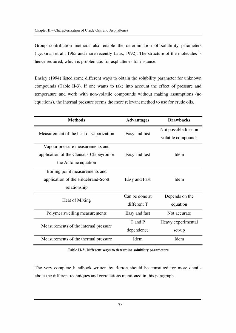
Chapter II – Characterization of Crude Oils and Asphaltenes
73
Group contribution methods also enable the determination of solubility parameters
(Lyckman et al., 1965 and more recently Laux, 1992). The structure of the molecules is
hence required, which is problematic for asphaltenes for instance.
Ensley (1994) listed some different ways to obtain the solubility parameter for unknown
compounds (Table II-3). If one wants to take into account the effect of pressure and
temperature and work with non-volatile compounds without making assumptions (no
equations), the internal pressure seems the more relevant method to use for crude oils.
Methods Advantages Drawbacks
Measurement of the heat of vaporization Easy and fast Not possible for non
volatile compounds
Vapour pressure measurements and
application of the Clausius-Clapeyron or
the Antoine equation
Easy and fast Idem
Boiling point measurements and
application of the Hildebrand-Scott
relationship
Easy and Fast Idem
Heat of Mixing Can be done at
different T
Depends on the
equation
Polymer swelling measurements Easy and fast Not accurate
Measurements of the internal pressure T and P
dependence
Heavy experimental
set-up
Measurements of the thermal pressure Idem Idem
Table II-3: Different ways to determine solubility parameters
The very complete handbook written by Barton should be consulted for more details
about the different techniques and correlations mentioned in this paragraph.
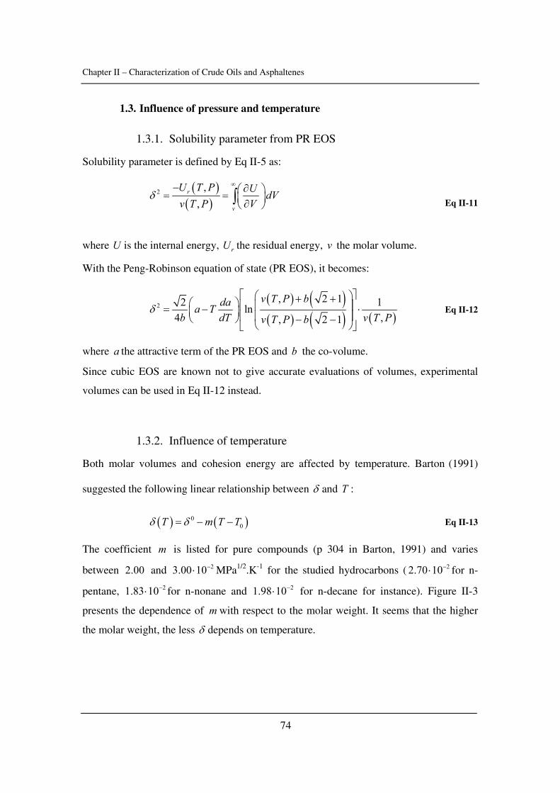
Chapter II – Characterization of Crude Oils and Asphaltenes
74
1.3. Influence of pressure and temperature
1.3.1. Solubility parameter from PR EOS
Solubility parameter is defined by Eq II-5 as:
( )( )
2 ,,
r
v
U T P U dVv T P V
δ∞− ∂⎛ ⎞= = ⎜ ⎟∂⎝ ⎠∫ Eq II-11
where U is the internal energy, rU the residual energy, v the molar volume.
With the Peng-Robinson equation of state (PR EOS), it becomes:
( ) ( )( ) ( ) ( )
2, 2 12 1ln
4 ,, 2 1
v T P bdaa Tb dT v T Pv T P b
δ⎡ ⎤⎛ ⎞+ +⎛ ⎞ ⎢ ⎥⎜ ⎟= − ⋅⎜ ⎟ ⎢ ⎥⎜ ⎟⎝ ⎠ − −⎝ ⎠⎣ ⎦
Eq II-12
where a the attractive term of the PR EOS and b the co-volume.
Since cubic EOS are known not to give accurate evaluations of volumes, experimental
volumes can be used in Eq II-12 instead.
1.3.2. Influence of temperature
Both molar volumes and cohesion energy are affected by temperature. Barton (1991)
suggested the following linear relationship between δ and T :
( ) ( )00T m T Tδ δ= − − Eq II-13
The coefficient m is listed for pure compounds (p 304 in Barton, 1991) and varies
between 2.00 and 23.00 10−⋅ MPa1/2.K-1 for the studied hydrocarbons ( 22.70 10−⋅ for n-
pentane, 21.83 10−⋅ for n-nonane and 21.98 10−⋅ for n-decane for instance). Figure II-3
presents the dependence of m with respect to the molar weight. It seems that the higher
the molar weight, the less δ depends on temperature.
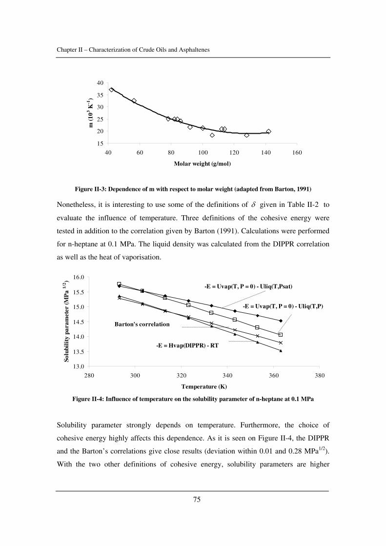
Chapter II – Characterization of Crude Oils and Asphaltenes
75
15
20
25
30
35
40
40 60 80 100 120 140 160
Molar weight (g/mol)
m (1
03 K-1
)
Figure II-3: Dependence of m with respect to molar weight (adapted from Barton, 1991)
Nonetheless, it is interesting to use some of the definitions of δ given in Table II-2 to
evaluate the influence of temperature. Three definitions of the cohesive energy were
tested in addition to the correlation given by Barton (1991). Calculations were performed
for n-heptane at 0.1 MPa. The liquid density was calculated from the DIPPR correlation
as well as the heat of vaporisation.
13.0
13.5
14.0
14.5
15.0
15.5
16.0
280 300 320 340 360 380
Temperature (K)
Solu
bili
ty p
aram
eter
(MP
a 1/
2 )
-E = Uvap(T, P = 0) - Uliq(T,Psat)
-E = Uvap(T, P = 0) - Uliq(T,P)
-E = Hvap(DIPPR) - RT
Barton's correlation
Figure II-4: Influence of temperature on the solubility parameter of n-heptane at 0.1 MPa
Solubility parameter strongly depends on temperature. Furthermore, the choice of
cohesive energy highly affects this dependence. As it is seen on Figure II-4, the DIPPR
and the Barton’s correlations give close results (deviation within 0.01 and 0.28 MPa1/2).
With the two other definitions of cohesive energy, solubility parameters are higher
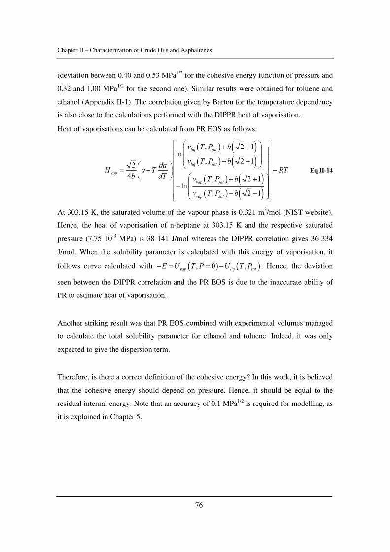
Chapter II – Characterization of Crude Oils and Asphaltenes
76
(deviation between 0.40 and 0.53 MPa1/2 for the cohesive energy function of pressure and
0.32 and 1.00 MPa1/2 for the second one). Similar results were obtained for toluene and
ethanol (Appendix II-1). The correlation given by Barton for the temperature dependency
is also close to the calculations performed with the DIPPR heat of vaporisation.
Heat of vaporisations can be calculated from PR EOS as follows:
( ) ( )( ) ( )
( ) ( )( ) ( )
, 2 1ln
, 2 124 , 2 1
ln, 2 1
liq sat
liq sat
vap
vap sat
vap sat
v T P b
v T P bdaH a T RTb dT v T P b
v T P b
⎡ ⎤⎛ ⎞+ +⎢ ⎥⎜ ⎟⎢ ⎥⎜ ⎟− −⎝ ⎠⎛ ⎞ ⎢ ⎥= − +⎜ ⎟ ⎢ ⎥⎝ ⎠ ⎛ ⎞+ +⎢ ⎥⎜ ⎟−⎢ ⎥⎜ ⎟− −⎢ ⎥⎝ ⎠⎣ ⎦
Eq II-14
At 303.15 K, the saturated volume of the vapour phase is 0.321 m3/mol (NIST website).
Hence, the heat of vaporisation of n-heptane at 303.15 K and the respective saturated
pressure (7.75 10-3 MPa) is 38 141 J/mol whereas the DIPPR correlation gives 36 334
J/mol. When the solubility parameter is calculated with this energy of vaporisation, it
follows curve calculated with ( ) ( ), 0 ,vap liq satE U T P U T P− = = − . Hence, the deviation
seen between the DIPPR correlation and the PR EOS is due to the inaccurate ability of
PR to estimate heat of vaporisation.
Another striking result was that PR EOS combined with experimental volumes managed
to calculate the total solubility parameter for ethanol and toluene. Indeed, it was only
expected to give the dispersion term.
Therefore, is there a correct definition of the cohesive energy? In this work, it is believed
that the cohesive energy should depend on pressure. Hence, it should be equal to the
residual internal energy. Note that an accuracy of 0.1 MPa1/2 is required for modelling, as
it is explained in Chapter 5.
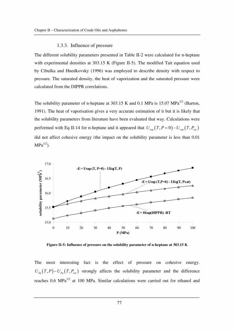
Chapter II – Characterization of Crude Oils and Asphaltenes
77
1.3.3. Influence of pressure
The different solubility parameters presented in Table II-2 were calculated for n-heptane
with experimental densities at 303.15 K (Figure II-5). The modified Tait equation used
by Cibulka and Hnedkovsky (1996) was employed to describe density with respect to
pressure. The saturated density, the heat of vaporization and the saturated pressure were
calculated from the DIPPR correlations.
The solubility parameter of n-heptane at 303.15 K and 0.1 MPa is 15.07 MPa1/2 (Barton,
1991). The heat of vaporisation gives a very accurate estimation of it but it is likely that
the solubility parameters from literature have been evaluated that way. Calculations were
performed with Eq II-14 for n-heptane and it appeared that ( ) ( ), 0 ,vap vap satU T P U T P= −
did not affect cohesive energy (the impact on the solubility parameter is less than 0.01
MPa1/2).
15.0
15.5
16.0
16.5
17.0
0 10 20 30 40 50 60 70 80 90 100P (MPa)
solu
bilit
y pa
ram
eter
(MPa1/
2 )
-E = Uvap (T,P=0) - Uliq(T, Psat)
-E = Uvap (T, P=0) - Uliq(T, P)
-E = Hvap(DIPPR) -RT
Figure II-5: Influence of pressure on the solubility parameter of n-heptane at 303.15 K
The most interesting fact is the effect of pressure on cohesive energy.
( ) ( ), ,liq liq satU T P U T P− strongly affects the solubility parameter and the difference
reaches 0.6 MPa1/2 at 100 MPa. Similar calculations were carried out for ethanol and
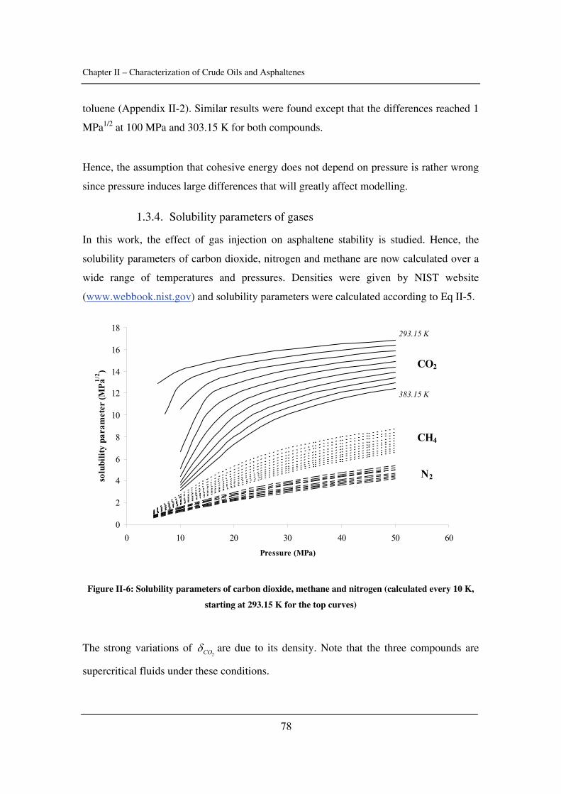
Chapter II – Characterization of Crude Oils and Asphaltenes
78
toluene (Appendix II-2). Similar results were found except that the differences reached 1
MPa1/2 at 100 MPa and 303.15 K for both compounds.
Hence, the assumption that cohesive energy does not depend on pressure is rather wrong
since pressure induces large differences that will greatly affect modelling.
1.3.4. Solubility parameters of gases
In this work, the effect of gas injection on asphaltene stability is studied. Hence, the
solubility parameters of carbon dioxide, nitrogen and methane are now calculated over a
wide range of temperatures and pressures. Densities were given by NIST website
(www.webbook.nist.gov) and solubility parameters were calculated according to Eq II-5.
0
2
4
6
8
10
12
14
16
18
0 10 20 30 40 50 60
Pressure (MPa)
solu
bilit
y pa
ram
eter
(MPa
1/2 ) CO2
N2
CH4
293.15 K
383.15 K
Figure II-6: Solubility parameters of carbon dioxide, methane and nitrogen (calculated every 10 K,
starting at 293.15 K for the top curves)
The strong variations of 2COδ are due to its density. Note that the three compounds are
supercritical fluids under these conditions.
Chapter II – Characterization of Crude Oils and Asphaltenes
79
1.4. Conclusion
The various definitions of cohesive energy induced many definitions and databases of
solubility parameters for pure compounds. The heat of vaporisation can be used if it is the
one given at the saturated pressure. The effects of temperature and pressure are both
important and should be taken into account. When PR EOS is combined to experimental
molar volumes, the total δ is believed to be properly estimated.
Chapter II – Characterization of Crude Oils and Asphaltenes
80
2. Solubility parameter of crude oil
2.1. Internal pressure, an alternative
The internal pressure π is defined as follows:
PTPTPT
VU
T
P
VT
−=−⎟⎠⎞
⎜⎝⎛
∂∂
=⎟⎠⎞
⎜⎝⎛
∂∂
=κα
π Eq II-15
where P
P TV
V⎟⎠⎞
⎜⎝⎛
∂∂
=1α is the thermal expansivity and
TT P
VV
⎟⎠⎞
⎜⎝⎛
∂∂
−=1κ the isothermal
compressibility.
The difference between internal pressure and solubility parameter is not that simple: these
two notions describe the same phenomenon, i.e. the cohesion of a liquid but not in the
same way. The cohesive energy density is a measure of the total molecular cohesion per
unit volume contrary to the internal pressure, which is a measure of the change in internal
energy of a liquid as it experiences a small isothermal expansion. Such a differential
change in volume does not necessarily disrupt all intermolecular interactions to an equal
extent. The interactions most affected include repulsion, dispersion and weak dipole
processes. In other words, a small volume expansion has a disruptive effect on these
interactions, which may be equivalent to that of vaporisation (Barton, 1983).
One can attempt to link these two notions using the typical Mie’s form of the
intermolecular potential:
mnRA Vb
VaUUU +−=+= Eq II-16
where AU is the attractive energy, RU the repulsive term, V the molar volume, a , b ,
m and n are constants. The repulsive term RU is only significant for highly compressed
liquids so, at low pressures, we have:
nA VaUU −== Eq II-17
Using Eq II-7 and Eq II-17, one obtains:
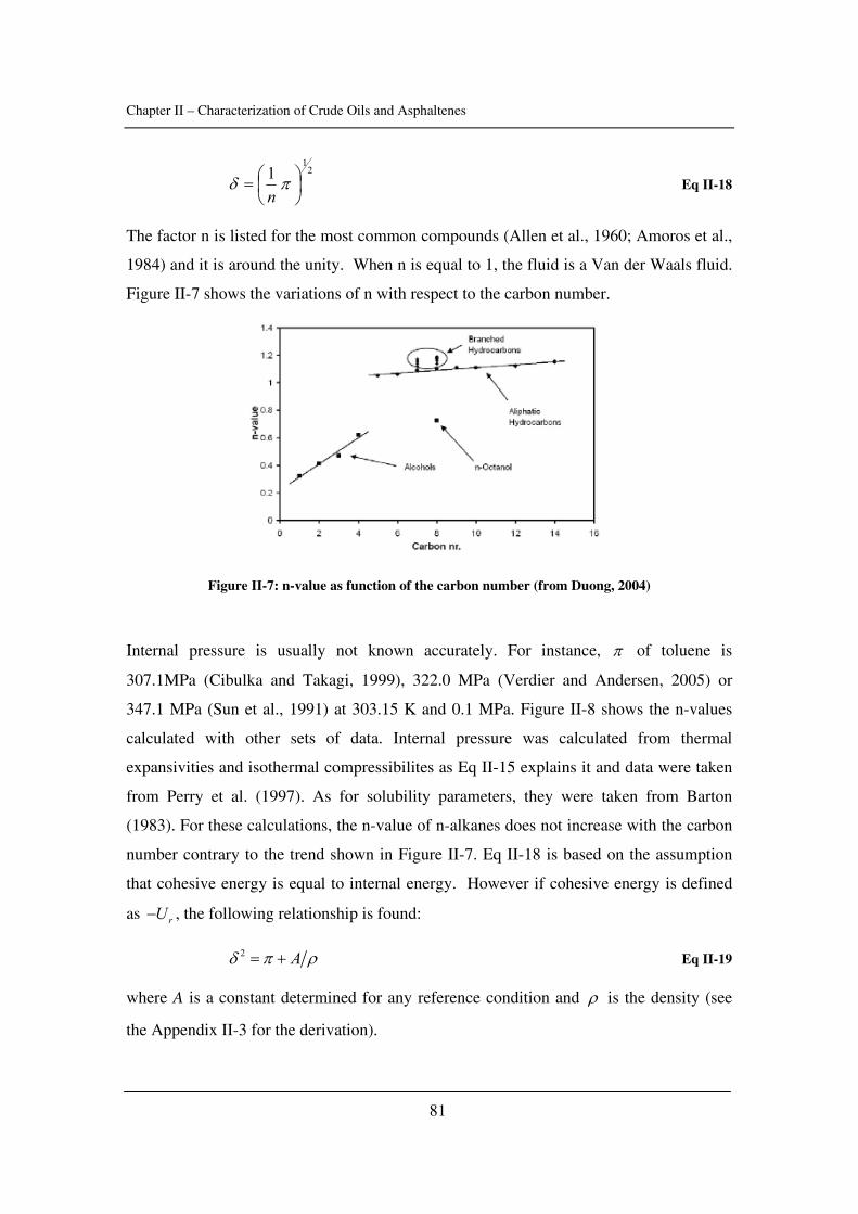
Chapter II – Characterization of Crude Oils and Asphaltenes
81
21
1⎟⎠⎞
⎜⎝⎛= πδ
n Eq II-18
The factor n is listed for the most common compounds (Allen et al., 1960; Amoros et al.,
1984) and it is around the unity. When n is equal to 1, the fluid is a Van der Waals fluid.
Figure II-7 shows the variations of n with respect to the carbon number.
Figure II-7: n-value as function of the carbon number (from Duong, 2004)
Internal pressure is usually not known accurately. For instance, π of toluene is
307.1MPa (Cibulka and Takagi, 1999), 322.0 MPa (Verdier and Andersen, 2005) or
347.1 MPa (Sun et al., 1991) at 303.15 K and 0.1 MPa. Figure II-8 shows the n-values
calculated with other sets of data. Internal pressure was calculated from thermal
expansivities and isothermal compressibilites as Eq II-15 explains it and data were taken
from Perry et al. (1997). As for solubility parameters, they were taken from Barton
(1983). For these calculations, the n-value of n-alkanes does not increase with the carbon
number contrary to the trend shown in Figure II-7. Eq II-18 is based on the assumption
that cohesive energy is equal to internal energy. However if cohesive energy is defined
as rU− , the following relationship is found:
2 Aδ π ρ= + Eq II-19
where A is a constant determined for any reference condition and ρ is the density (see
the Appendix II-3 for the derivation).
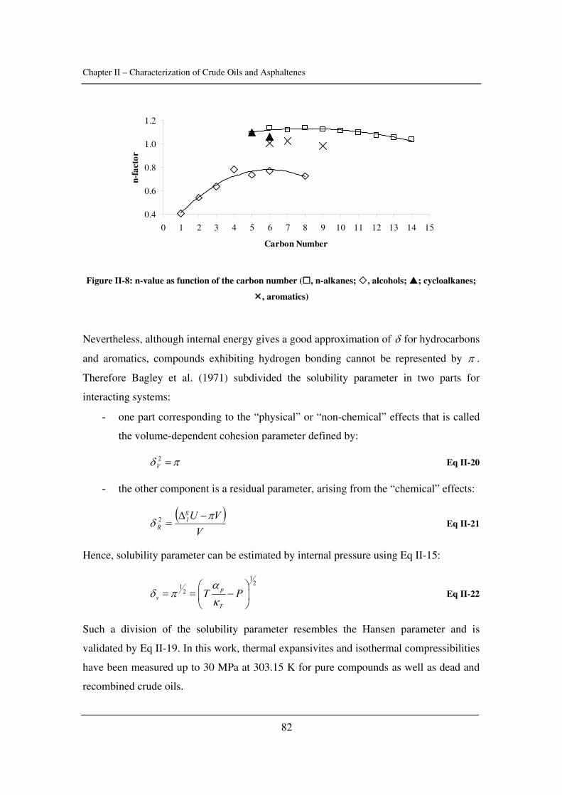
Chapter II – Characterization of Crude Oils and Asphaltenes
82
0.4
0.6
0.8
1.0
1.2
0 1 2 3 4 5 6 7 8 9 10 11 12 13 14 15
Carbon Number
n-fa
ctor
Figure II-8: n-value as function of the carbon number ( , n-alkanes; , alcohols; ; cycloalkanes;
, aromatics)
Nevertheless, although internal energy gives a good approximation of δ for hydrocarbons
and aromatics, compounds exhibiting hydrogen bonding cannot be represented by π .
Therefore Bagley et al. (1971) subdivided the solubility parameter in two parts for
interacting systems:
- one part corresponding to the “physical” or “non-chemical” effects that is called
the volume-dependent cohesion parameter defined by:
πδ =2V Eq II-20
- the other component is a residual parameter, arising from the “chemical” effects:
( )V
VUgl
Rπ
δ−Δ
=2 Eq II-21
Hence, solubility parameter can be estimated by internal pressure using Eq II-15:
121
2 pv
T
T Pα
δ πκ
⎛ ⎞= = −⎜ ⎟
⎝ ⎠ Eq II-22
Such a division of the solubility parameter resembles the Hansen parameter and is
validated by Eq II-19. In this work, thermal expansivites and isothermal compressibilities
have been measured up to 30 MPa at 303.15 K for pure compounds as well as dead and
recombined crude oils.
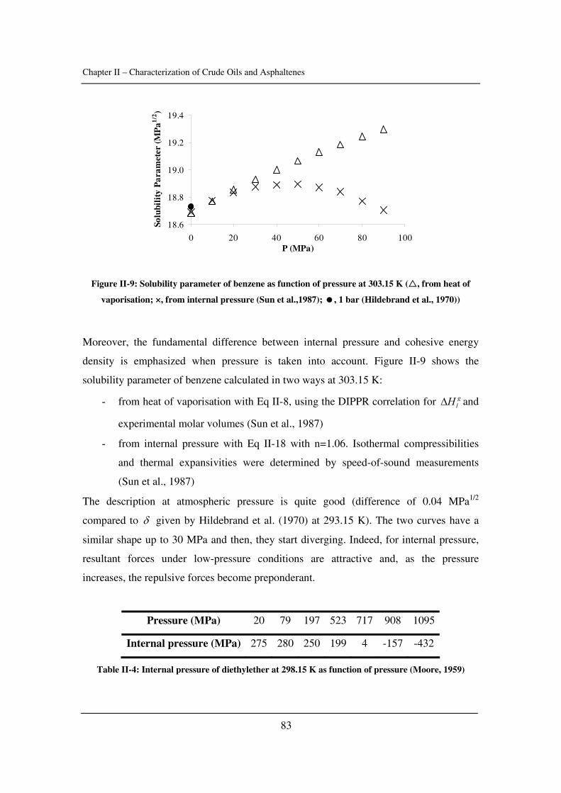
Chapter II – Characterization of Crude Oils and Asphaltenes
83
18.6
18.8
19.0
19.2
19.4
0 20 40 60 80 100P (MPa)
Solu
bili
ty P
aram
eter
(MP
a1/2 )
Figure II-9: Solubility parameter of benzene as function of pressure at 303.15 K ( , from heat of
vaporisation; ×, from internal pressure (Sun et al.,1987); , 1 bar (Hildebrand et al., 1970))
Moreover, the fundamental difference between internal pressure and cohesive energy
density is emphasized when pressure is taken into account. Figure II-9 shows the
solubility parameter of benzene calculated in two ways at 303.15 K:
- from heat of vaporisation with Eq II-8, using the DIPPR correlation for glHΔ and
experimental molar volumes (Sun et al., 1987)
- from internal pressure with Eq II-18 with n=1.06. Isothermal compressibilities
and thermal expansivities were determined by speed-of-sound measurements
(Sun et al., 1987)
The description at atmospheric pressure is quite good (difference of 0.04 MPa1/2
compared to δ given by Hildebrand et al. (1970) at 293.15 K). The two curves have a
similar shape up to 30 MPa and then, they start diverging. Indeed, for internal pressure,
resultant forces under low-pressure conditions are attractive and, as the pressure
increases, the repulsive forces become preponderant.
Pressure (MPa) 20 79 197 523 717 908 1095
Internal pressure (MPa) 275 280 250 199 4 -157 -432
Table II-4: Internal pressure of diethylether at 298.15 K as function of pressure (Moore, 1959)
Chapter II – Characterization of Crude Oils and Asphaltenes
84
Table II-4 illustrates this effect of pressure on internal pressure for diethyl ether at 298.15
K (Moore, 1959) For moderate increases in pressure, the internal pressure first increases
only slightly and then decreases slowly but as P exceeds 500 MPa, the internal pressure
begins to decrease rapidly, and goes to large negative values as the liquid is further
compressed.
Therefore, though internal pressure and solubility parameter are related to the cohesive
energy, they behave differently when hydrogen bonding or pressure are at stake for
instance.
2.2. Internal pressure of pure compounds
The experimental procedure is detailed in Verdier and Andersen (2005) (presented in
Appendix II-4). Nevetheless, a short description will be given.
Scanning transitiometry was used to measure thermal expansivities. This method was
proposed by Randzio in 1985. A fluid is isothermally compressed or decompressed in a
calorimeter and the heat released is proportional to its thermal expansivity as follows:
( )dtdPTV
dtQ
VPT
ααδ−−= Eq II-23
where ( )T
dTQδ is the rate of heat measured by the microcalorimeter, pα the thermal
expansivity of the fluid under investigation, Vα the thermal expansivity of the stainless
steel, V the volume of the cell, T the temperature and dTdP the rate of increase in
pressure.
In this work, a LKB 2277 Bio Monitor calorimeter was modified to stand high-pressures.
An automatic high-pressure syringe pump (ISCO 260 D) was used to compress and
decompress the fluid. Unfortunately, this calorimeter does not permit scanning in
temperatures. Thermal expansivities of several pure compounds were measured up to 30
MPa and at 303.15 K. The deviation to literature data was within 2%.
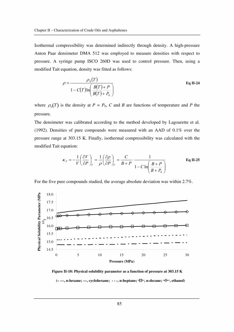
Chapter II – Characterization of Crude Oils and Asphaltenes
85
Isothermal compressibility was determined indirectly through density. A high-pressure
Anton Paar densimeter DMA 512 was employed to measure densities with respect to
pressure. A syringe pump ISCO 260D was used to control pressure. Then, using a
modified Tait equation, density was fitted as follows:
( )
( ) ( )( ) ⎟⎟
⎠
⎞⎜⎜⎝
⎛++
−
=
0
0
ln1PTBPTBTC
Tρρ Eq II-24
where ρ0 T( ) is the density at P = P0, C and B are functions of temperature and P the
pressure.
The densimeter was calibrated according to the method developed by Lagourette et al.
(1992). Densities of pure compounds were measured with an AAD of 0.1% over the
pressure range at 303.15 K. Finally, isothermal compressibility was calculated with the
modified Tait equation:
⎟⎟⎠
⎞⎜⎜⎝
⎛++
−⋅
+=⎟
⎠⎞
⎜⎝⎛
∂∂
=⎟⎠⎞
⎜⎝⎛
∂∂
−=
0
ln1
111
PBPBC
PBC
PPV
V TTT
ρρ
κ Eq II-25
For the five pure compounds studied, the average absolute deviation was within 2.7%.
14.5
15.0
15.5
16.0
16.5
17.0
17.5
18.0
0 5 10 15 20 25 30
Pressure (MPa)
Phy
sica
l Sol
ubil
ity
Par
amet
er (M
Pa
1/2 )
Figure II-10: Physical solubility parameter as a function of pressure at 303.15 K
(– —, n-hexane; —, cyclohexane; - - -, n-heptane; , n-decane; , ethanol)
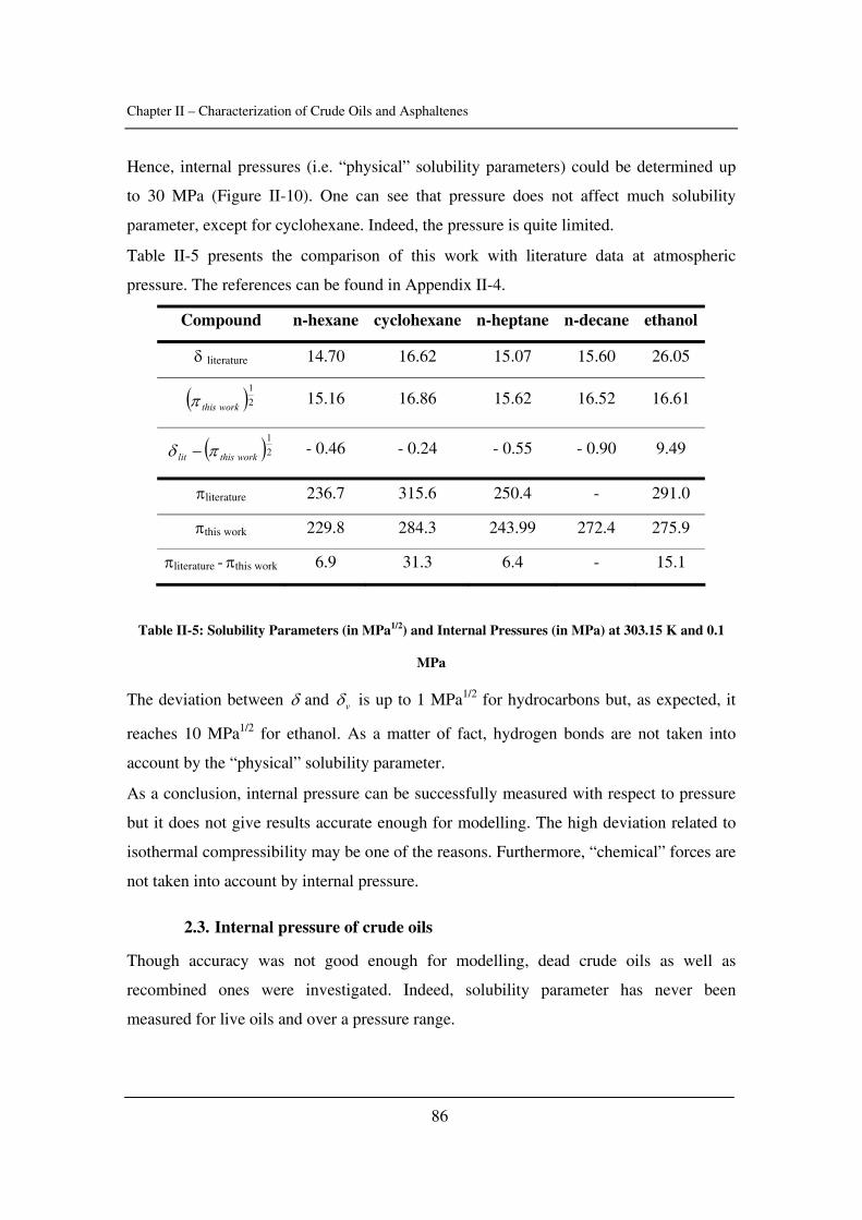
Chapter II – Characterization of Crude Oils and Asphaltenes
86
Hence, internal pressures (i.e. “physical” solubility parameters) could be determined up
to 30 MPa (Figure II-10). One can see that pressure does not affect much solubility
parameter, except for cyclohexane. Indeed, the pressure is quite limited.
Table II-5 presents the comparison of this work with literature data at atmospheric
pressure. The references can be found in Appendix II-4.
Compound n-hexane cyclohexane n-heptane n-decane ethanol
δ literature 14.70 16.62 15.07 15.60 26.05
( )21
workthisπ 15.16 16.86 15.62 16.52 16.61
( )21
workthislit πδ − - 0.46 - 0.24 - 0.55 - 0.90 9.49
πliterature 236.7 315.6 250.4 - 291.0
πthis work 229.8 284.3 243.99 272.4 275.9
πliterature - πthis work 6.9 31.3 6.4 - 15.1
Table II-5: Solubility Parameters (in MPa1/2) and Internal Pressures (in MPa) at 303.15 K and 0.1
MPa
The deviation between δ and vδ is up to 1 MPa1/2 for hydrocarbons but, as expected, it
reaches 10 MPa1/2 for ethanol. As a matter of fact, hydrogen bonds are not taken into
account by the “physical” solubility parameter.
As a conclusion, internal pressure can be successfully measured with respect to pressure
but it does not give results accurate enough for modelling. The high deviation related to
isothermal compressibility may be one of the reasons. Furthermore, “chemical” forces are
not taken into account by internal pressure.
2.3. Internal pressure of crude oils
Though accuracy was not good enough for modelling, dead crude oils as well as
recombined ones were investigated. Indeed, solubility parameter has never been
measured for live oils and over a pressure range.
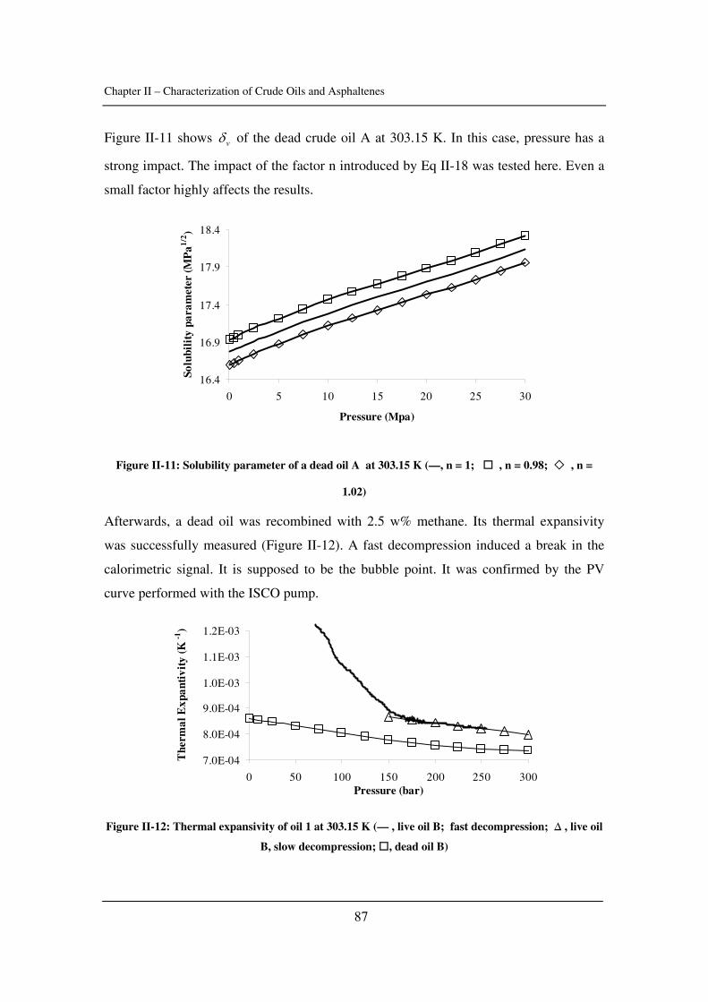
Chapter II – Characterization of Crude Oils and Asphaltenes
87
Figure II-11 shows vδ of the dead crude oil A at 303.15 K. In this case, pressure has a
strong impact. The impact of the factor n introduced by Eq II-18 was tested here. Even a
small factor highly affects the results.
16.4
16.9
17.4
17.9
18.4
0 5 10 15 20 25 30
Pressure (Mpa)
Solu
bili
ty p
aram
eter
(MP
a1/2 )
Figure II-11: Solubility parameter of a dead oil A at 303.15 K (—, n = 1; , n = 0.98; , n =
1.02)
Afterwards, a dead oil was recombined with 2.5 w% methane. Its thermal expansivity
was successfully measured (Figure II-12). A fast decompression induced a break in the
calorimetric signal. It is supposed to be the bubble point. It was confirmed by the PV
curve performed with the ISCO pump.
7.0E-04
8.0E-04
9.0E-04
1.0E-03
1.1E-03
1.2E-03
0 50 100 150 200 250 300Pressure (bar)
The
rmal
Exp
anti
vity
(K -1
)
Figure II-12: Thermal expansivity of oil 1 at 303.15 K (— , live oil B; fast decompression; ∆ , live oil
B, slow decompression; , dead oil B)
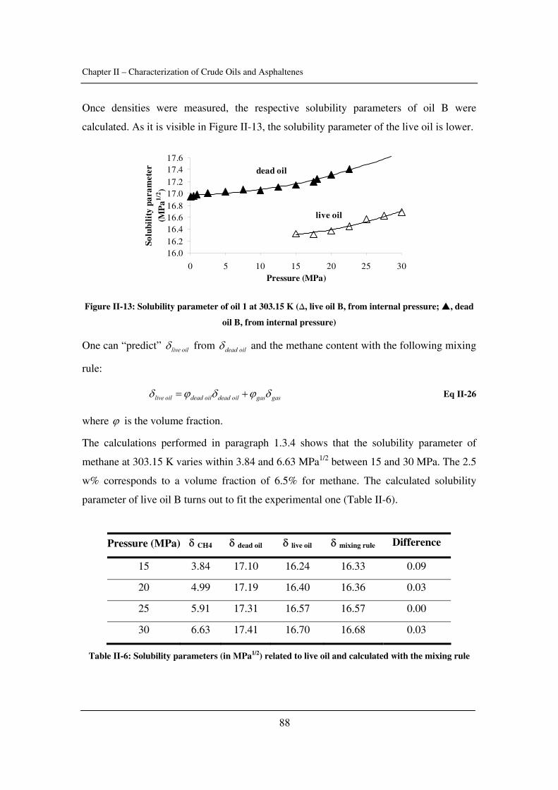
Chapter II – Characterization of Crude Oils and Asphaltenes
88
Once densities were measured, the respective solubility parameters of oil B were
calculated. As it is visible in Figure II-13, the solubility parameter of the live oil is lower.
16.016.216.416.616.817.017.217.417.6
0 5 10 15 20 25 30Pressure (MPa)
Solu
bili
ty p
aram
eter
(MP
a1/2 )
dead oil
live oil
Figure II-13: Solubility parameter of oil 1 at 303.15 K (∆, live oil B, from internal pressure; , dead
oil B, from internal pressure)
One can “predict” live oilδ from dead oilδ and the methane content with the following mixing
rule:
live oil dead oil dead oil gas gasδ ϕ δ ϕ δ= + Eq II-26
where ϕ is the volume fraction.
The calculations performed in paragraph 1.3.4 shows that the solubility parameter of
methane at 303.15 K varies within 3.84 and 6.63 MPa1/2 between 15 and 30 MPa. The 2.5
w% corresponds to a volume fraction of 6.5% for methane. The calculated solubility
parameter of live oil B turns out to fit the experimental one (Table II-6).
Pressure (MPa) δ CH4 δ dead oil δ live oil δ mixing rule Difference
15 3.84 17.10 16.24 16.33 0.09
20 4.99 17.19 16.40 16.36 0.03
25 5.91 17.31 16.57 16.57 0.00
30 6.63 17.41 16.70 16.68 0.03
Table II-6: Solubility parameters (in MPa1/2) related to live oil and calculated with the mixing rule
Chapter II – Characterization of Crude Oils and Asphaltenes
89
2.4. Conclusion
Internal pressures of dead and live oils can be successfully measured up to 30 MPa.
However, by definition, solubility parameter and internal pressure are different. Hence,
such measurements turn out to be incompatible with modelling since a high accuracy is
expected. Nonetheless, it is the first time that solubility parameters of oils have been
measured. Modelling of the solubility parameter has been performed with PR EOS for
this crude oil after it has been characterised but the deviation was quite high (up to 4.9
MPa1/2). More details are available in Appendix II-5 about this modelling.
Chapter II – Characterization of Crude Oils and Asphaltenes
90
3. Characterization of asphaltenes
The issues about asphaltene characterisation were introduced in Chapter 1, paragraph 1.3.
The polydisperse nature of asphaltenes makes any characterisation difficult. However, in
this paragraph, solubility parameters and critical constants were determined for several
asphaltenes in solution.
3.1. Solubility parameter of asphaltenes
3.1.1. Literature survey
The determination of the solubility parameters of asphaltenes is uncertain in most cases.
Hirschberg et al. (1984) used titration experiments to determine asphaltene solubility
parameters, assuming a molar volume. They found a value of 19.50 MPa1/2 and a small
temperature dependence when fitting their data. Wang and Buckley (2001) used
asphaltene molar volume and solubility parameter as adjustable parameters in their
asphaltene solubility model. As for Yarranton and Masliyah (1996), they determined it by
fitting the model to one set of asphaltene-n-heptane-toluene titration curve. Could it be
done otherwise? Can a complex and polydisperse system be represented by a single
parameter? Nevertheless, several techniques are available to determine this parameter for
asphaltenes. They are based on:
- Miscibility (Lian, 1994): here, the miscibility of asphaltenes is measured in
various solvents and a solubility profile is obtained. Hence, a range of solubility
parameters is obtained. Lian reports solubility parameters ranging between 17.6
and 21.3 MPa1/2.
- Titration (Hirschberg et al., 1984; Andersen, 1999): Andersen states that, if one
plots precipitant oilVV vs. solvent oilVV , both the intercept and the slope give access to
the solubility parameter of the crude oil oδ and to a critical one crδ . Empirically,
in polymer chemistry, the solubility parameter of asphaltenes is such as
4a crδ δ= + (in MPa1/2). Eighteen crude oils were investigated and the calculated
aδ are within 19 and 22 MPa1/2 at room conditions.
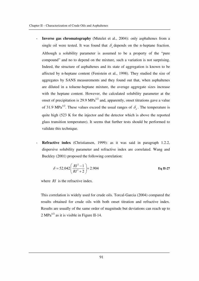
Chapter II – Characterization of Crude Oils and Asphaltenes
91
- Inverse gas chromatography (Mutelet et al., 2004): only asphaltenes from a
single oil were tested. It was found that aδ depends on the n-heptane fraction.
Although a solubility parameter is assumed to be a property of the “pure
compound” and no to depend on the mixture, such a variation is not surprising.
Indeed, the structure of asphaltenes and its state of aggregation is known to be
affected by n-heptane content (Fenistein et al., 1998). They studied the size of
aggregates by SANS measurements and they found out that, when asphaltenes
are diluted in a toluene-heptane mixture, the average aggregate sizes increase
with the heptane content. However, the calculated solubility parameter at the
onset of precipitation is 29.9 MPa1/2 and, apparently, onset titrations gave a value
of 31.9 MPa1/2. These values exceed the usual ranges of aδ . The temperature is
quite high (523 K for the injector and the detector which is above the reported
glass transition temperature). It seems that further tests should be performed to
validate this technique.
- Refractive index (Christiansen, 1999): as it was said in paragraph 1.2.2,
dispersive solubility parameter and refractive index are correlated. Wang and
Buckley (2001) proposed the following correlation:
2
2
152.042 2.9042
RIRI
δ⎛ ⎞−
= +⎜ ⎟+⎝ ⎠ Eq II-27
where RI is the refractive index.
This correlation is widely used for crude oils. Torcal-Garcia (2004) compared the
results obtained for crude oils with both onset titration and refractive index.
Results are usually of the same order of magnitude but deviations can reach up to
2 MPa1/2 as it is visible in Figure II-14.
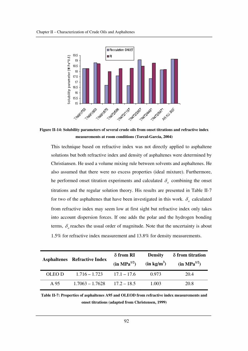
Chapter II – Characterization of Crude Oils and Asphaltenes
92
Figure II-14: Solubility parameters of several crude oils from onset titrations and refractive index
measurements at room conditions (Torcal-Garcia, 2004)
This technique based on refractive index was not directly applied to asphaltene
solutions but both refractive index and density of asphaltenes were determined by
Christiansen. He used a volume mixing rule between solvents and asphaltenes. He
also assumed that there were no excess properties (ideal mixture). Furthermore,
he performed onset titration experiments and calculated aδ combining the onset
titrations and the regular solution theory. His results are presented in Table II-7
for two of the asphaltenes that have been investigated in this work. aδ calculated
from refractive index may seem low at first sight but refractive index only takes
into account dispersion forces. If one adds the polar and the hydrogen bonding
terms, aδ reaches the usual order of magnitude. Note that the uncertainty is about
1.5% for refractive index measurement and 13.8% for density measurements.
Asphaltenes Refractive Index δ from RI
(in MPa1/2)
Density
(in kg/m3)
δ from titration
(in MPa1/2)
OLEO D 1.716 – 1.723 17.1 – 17.6 0.973 20.4
A 95 1.7063 – 1.7628 17.2 – 18.5 1.003 20.8
Table II-7: Properties of asphaltenes A95 and OLEOD from refractive index measurements and
onset titrations (adapted from Christensen, 1999)
Chapter II – Characterization of Crude Oils and Asphaltenes
93
- Correlations (Laux, 1992): Laux developed a correlation taking into account the
hetero-atom content, the carbon number and the hydrogen deficit. Two
asphaltenes were tested with this method and the respective solubility parameters
are 18.68 and 19.35 MPa1/2, which is in the expected range. This method has not
been very much used. Indeed, a complete chemical analysis is required and the
temperature dependence is not taken into account.
So, a few techniques exist to evaluate the solubility parameter of asphaltenes. However,
they are either inaccurate (miscibility) or based on strong assumption (ideal solution for
the refractive index) or seem to give high results (chromatography).
3.1.2. Partial volumes and regular solution theory
In this work, a simple and fast technique, based on density measurements of asphaltenes
dissolved in several solvents, was applied to determine the solubility parameter of
asphaltenes. The input parameters are the internal and solubility parameters of the pure
solvents at 0.1 MPa and the desired temperature. This procedure had been used by Liron
and Cohen (1983) for compounds of pharmaceutical relevance such as cholesterol in
various solvents (toluene, carbon tetrachloride, chlorobenzene, chloroform and
nitrobenzene).
Consider a binary constituted of a solvent 1 and a solute 2. According to Hildebrand and
Dymond (1967), introducing molecules of solute in the solvent causes microscopic
regions of weakness and expansion until enough energy has been absorbed to restore the
local internal pressure to the bulk internal pressure. Accordingly, it can be written:
( ) 0221
022 EEvv −=− π Eq II-28
where 2v is the partial molar volume, 02v is the molar volume of the pure solute, 1π the
internal pressure of the solvent 1 and 022 EE − is the partial molar energy of transferring a
mole of liquid solute 2 from pure liquid to solution.
It is assumed that internal pressure is unchanged by the small amount of solute introduced
(Hildebrand et al., 1970). This equation has no theoretical background but, quoting
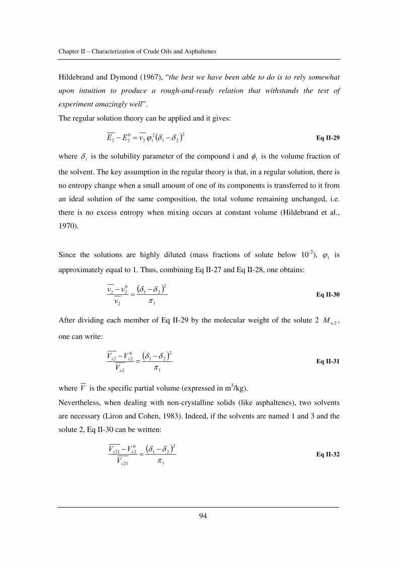
Chapter II – Characterization of Crude Oils and Asphaltenes
94
Hildebrand and Dymond (1967), “the best we have been able to do is to rely somewhat
upon intuition to produce a rough-and-ready relation that withstands the test of
experiment amazingly well”.
The regular solution theory can be applied and it gives:
( )221
212
022 δδϕ −=− vEE Eq II-29
where iδ is the solubility parameter of the compound i and 1φ is the volume fraction of
the solvent. The key assumption in the regular theory is that, in a regular solution, there is
no entropy change when a small amount of one of its components is transferred to it from
an ideal solution of the same composition, the total volume remaining unchanged, i.e.
there is no excess entropy when mixing occurs at constant volume (Hildebrand et al.,
1970).
Since the solutions are highly diluted (mass fractions of solute below 10-2), 1ϕ is
approximately equal to 1. Thus, combining Eq II-27 and Eq II-28, one obtains:
( )1
221
2
022
πδδ −
=−v
vv Eq II-30
After dividing each member of Eq II-29 by the molecular weight of the solute 2 2wM ,
one can write:
( )1
221
2
022
πδδ −
=−
s
ss
VVV
Eq II-31
where V is the specific partial volume (expressed in m3/kg).
Nevertheless, when dealing with non-crystalline solids (like asphaltenes), two solvents
are necessary (Liron and Cohen, 1983). Indeed, if the solvents are named 1 and 3 and the
solute 2, Eq II-30 can be written:
( )
1
221
21
0221
πδδ −
=−
s
ss
VVV
Eq II-32
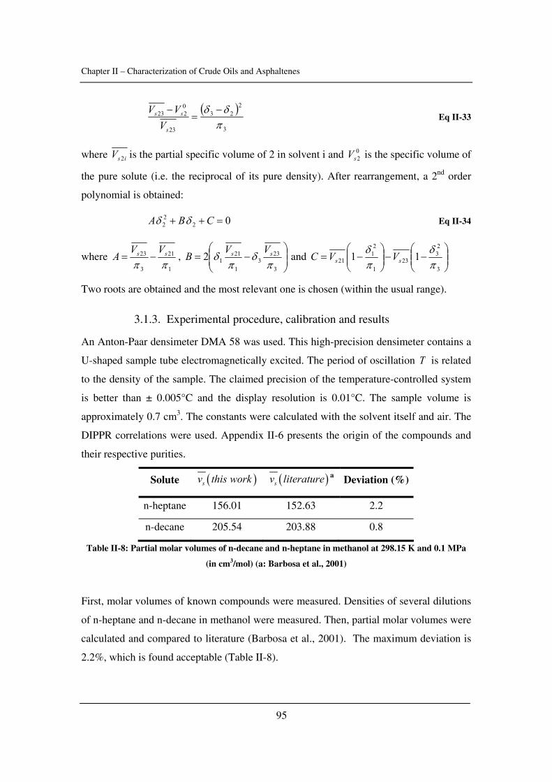
Chapter II – Characterization of Crude Oils and Asphaltenes
95
( )3
223
23
0223
πδδ −
=−
s
ss
VVV
Eq II-33
where isV 2 is the partial specific volume of 2 in solvent i and 02sV is the specific volume of
the pure solute (i.e. the reciprocal of its pure density). After rearrangement, a 2nd order
polynomial is obtained:
0222 =++ CBA δδ Eq II-34
where 1
21
3
23
ππss VVA −= , ⎟⎟
⎠
⎞⎜⎜⎝
⎛−=
3
233
1
2112
πδ
πδ ss VVB and ⎟⎟
⎠
⎞⎜⎜⎝
⎛−−⎟⎟
⎠
⎞⎜⎜⎝
⎛−=
3
23
231
21
21 11πδ
πδ
ss VVC
Two roots are obtained and the most relevant one is chosen (within the usual range).
3.1.3. Experimental procedure, calibration and results
An Anton-Paar densimeter DMA 58 was used. This high-precision densimeter contains a
U-shaped sample tube electromagnetically excited. The period of oscillation T is related
to the density of the sample. The claimed precision of the temperature-controlled system
is better than ± 0.005°C and the display resolution is 0.01°C. The sample volume is
approximately 0.7 cm3. The constants were calculated with the solvent itself and air. The
DIPPR correlations were used. Appendix II-6 presents the origin of the compounds and
their respective purities.
Solute ( )sv this work ( )sv literature a Deviation (%)
n-heptane 156.01 152.63 2.2
n-decane 205.54 203.88 0.8
Table II-8: Partial molar volumes of n-decane and n-heptane in methanol at 298.15 K and 0.1 MPa
(in cm3/mol) (a: Barbosa et al., 2001)
First, molar volumes of known compounds were measured. Densities of several dilutions
of n-heptane and n-decane in methanol were measured. Then, partial molar volumes were
calculated and compared to literature (Barbosa et al., 2001). The maximum deviation is
2.2%, which is found acceptable (Table II-8).
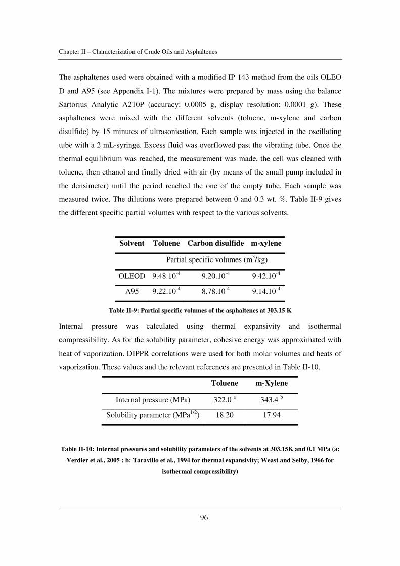
Chapter II – Characterization of Crude Oils and Asphaltenes
96
The asphaltenes used were obtained with a modified IP 143 method from the oils OLEO
D and A95 (see Appendix I-1). The mixtures were prepared by mass using the balance
Sartorius Analytic A210P (accuracy: 0.0005 g, display resolution: 0.0001 g). These
asphaltenes were mixed with the different solvents (toluene, m-xylene and carbon
disulfide) by 15 minutes of ultrasonication. Each sample was injected in the oscillating
tube with a 2 mL-syringe. Excess fluid was overflowed past the vibrating tube. Once the
thermal equilibrium was reached, the measurement was made, the cell was cleaned with
toluene, then ethanol and finally dried with air (by means of the small pump included in
the densimeter) until the period reached the one of the empty tube. Each sample was
measured twice. The dilutions were prepared between 0 and 0.3 wt. %. Table II-9 gives
the different specific partial volumes with respect to the various solvents.
Solvent Toluene Carbon disulfide m-xylene
Partial specific volumes (m3/kg)
OLEOD 9.48.10-4 9.20.10-4 9.42.10-4
A95 9.22.10-4 8.78.10-4 9.14.10-4
Table II-9: Partial specific volumes of the asphaltenes at 303.15 K
Internal pressure was calculated using thermal expansivity and isothermal
compressibility. As for the solubility parameter, cohesive energy was approximated with
heat of vaporization. DIPPR correlations were used for both molar volumes and heats of
vaporization. These values and the relevant references are presented in Table II-10.
Toluene m-Xylene
Internal pressure (MPa) 322.0 a 343.4 b
Solubility parameter (MPa1/2) 18.20 17.94
Table II-10: Internal pressures and solubility parameters of the solvents at 303.15K and 0.1 MPa (a:
Verdier et al., 2005 ; b: Taravillo et al., 1994 for thermal expansivity; Weast and Selby, 1966 for
isothermal compressibility)
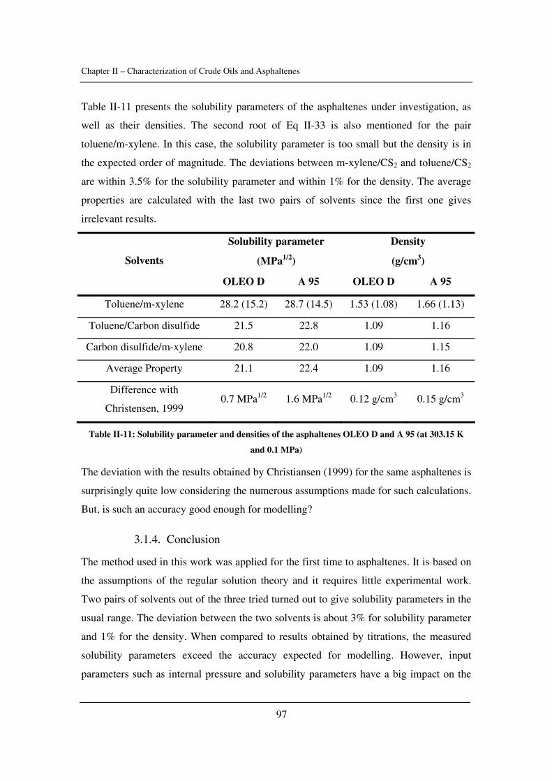
Chapter II – Characterization of Crude Oils and Asphaltenes
97
Table II-11 presents the solubility parameters of the asphaltenes under investigation, as
well as their densities. The second root of Eq II-33 is also mentioned for the pair
toluene/m-xylene. In this case, the solubility parameter is too small but the density is in
the expected order of magnitude. The deviations between m-xylene/CS2 and toluene/CS2
are within 3.5% for the solubility parameter and within 1% for the density. The average
properties are calculated with the last two pairs of solvents since the first one gives
irrelevant results.
Solubility parameter
(MPa1/2)
Density
(g/cm3) Solvents
OLEO D A 95 OLEO D A 95
Toluene/m-xylene 28.2 (15.2) 28.7 (14.5) 1.53 (1.08) 1.66 (1.13)
Toluene/Carbon disulfide 21.5 22.8 1.09 1.16
Carbon disulfide/m-xylene 20.8 22.0 1.09 1.15
Average Property 21.1 22.4 1.09 1.16
Difference with
Christensen, 1999 0.7 MPa1/2 1.6 MPa1/2 0.12 g/cm3 0.15 g/cm3
Table II-11: Solubility parameter and densities of the asphaltenes OLEO D and A 95 (at 303.15 K
and 0.1 MPa)
The deviation with the results obtained by Christiansen (1999) for the same asphaltenes is
surprisingly quite low considering the numerous assumptions made for such calculations.
But, is such an accuracy good enough for modelling?
3.1.4. Conclusion
The method used in this work was applied for the first time to asphaltenes. It is based on
the assumptions of the regular solution theory and it requires little experimental work.
Two pairs of solvents out of the three tried turned out to give solubility parameters in the
usual range. The deviation between the two solvents is about 3% for solubility parameter
and 1% for the density. When compared to results obtained by titrations, the measured
solubility parameters exceed the accuracy expected for modelling. However, input
parameters such as internal pressure and solubility parameters have a big impact on the
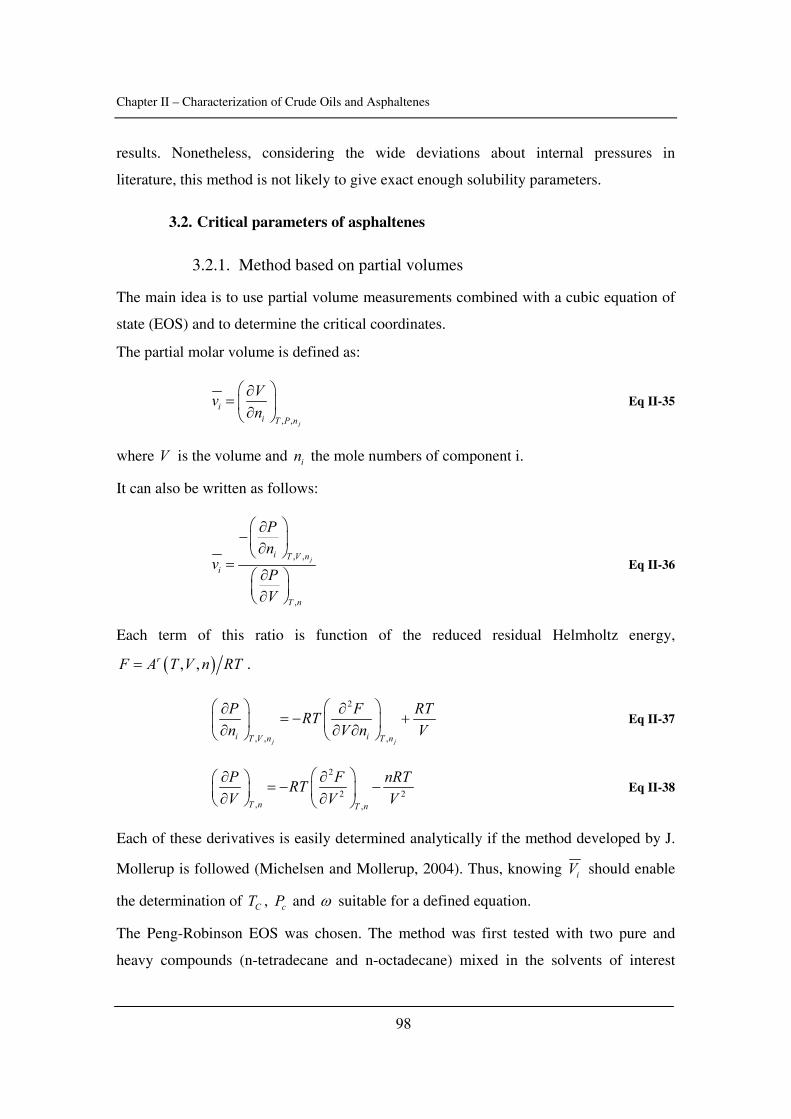
Chapter II – Characterization of Crude Oils and Asphaltenes
98
results. Nonetheless, considering the wide deviations about internal pressures in
literature, this method is not likely to give exact enough solubility parameters.
3.2. Critical parameters of asphaltenes
3.2.1. Method based on partial volumes
The main idea is to use partial volume measurements combined with a cubic equation of
state (EOS) and to determine the critical coordinates.
The partial molar volume is defined as:
, , j
ii T P n
Vvn
⎛ ⎞∂= ⎜ ⎟∂⎝ ⎠
Eq II-35
where V is the volume and in the mole numbers of component i.
It can also be written as follows:
, ,
,
ji T V n
i
T n
Pn
vPV
⎛ ⎞∂−⎜ ⎟∂⎝ ⎠
=∂⎛ ⎞
⎜ ⎟∂⎝ ⎠
Eq II-36
Each term of this ratio is function of the reduced residual Helmholtz energy,
( ), ,rF A T V n RT= .
2
, , ,j ji iT V n T n
P F RTRTn V n V
⎛ ⎞ ⎛ ⎞∂ ∂= − +⎜ ⎟ ⎜ ⎟∂ ∂ ∂⎝ ⎠ ⎝ ⎠
Eq II-37
2
2 2, ,T n T n
P F nRTRTV V V
⎛ ⎞∂ ∂⎛ ⎞ = − −⎜ ⎟⎜ ⎟∂ ∂⎝ ⎠ ⎝ ⎠ Eq II-38
Each of these derivatives is easily determined analytically if the method developed by J.
Mollerup is followed (Michelsen and Mollerup, 2004). Thus, knowing iV should enable
the determination of CT , cP and ω suitable for a defined equation.
The Peng-Robinson EOS was chosen. The method was first tested with two pure and
heavy compounds (n-tetradecane and n-octadecane) mixed in the solvents of interest
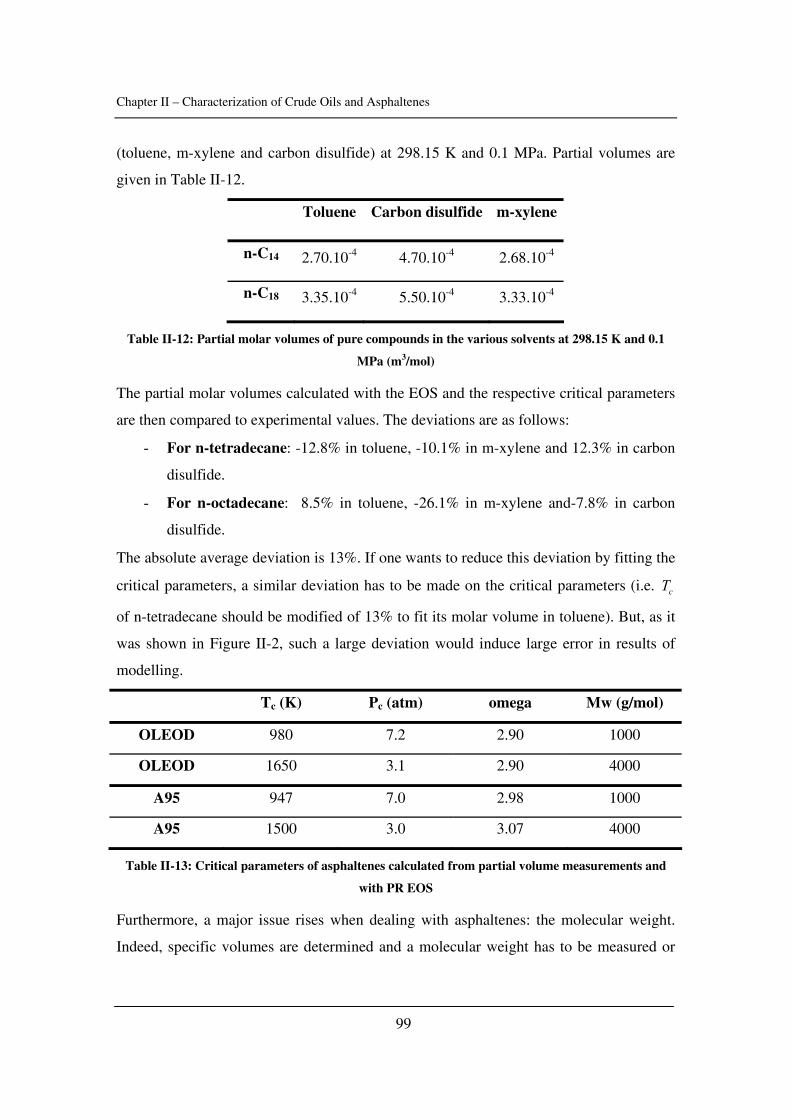
Chapter II – Characterization of Crude Oils and Asphaltenes
99
(toluene, m-xylene and carbon disulfide) at 298.15 K and 0.1 MPa. Partial volumes are
given in Table II-12.
Toluene Carbon disulfide m-xylene
n-C14 2.70.10-4 4.70.10-4 2.68.10-4
n-C18 3.35.10-4 5.50.10-4 3.33.10-4
Table II-12: Partial molar volumes of pure compounds in the various solvents at 298.15 K and 0.1
MPa (m3/mol)
The partial molar volumes calculated with the EOS and the respective critical parameters
are then compared to experimental values. The deviations are as follows:
- For n-tetradecane: -12.8% in toluene, -10.1% in m-xylene and 12.3% in carbon
disulfide.
- For n-octadecane: 8.5% in toluene, -26.1% in m-xylene and-7.8% in carbon
disulfide.
The absolute average deviation is 13%. If one wants to reduce this deviation by fitting the
critical parameters, a similar deviation has to be made on the critical parameters (i.e. cT
of n-tetradecane should be modified of 13% to fit its molar volume in toluene). But, as it
was shown in Figure II-2, such a large deviation would induce large error in results of
modelling.
Tc (K) Pc (atm) omega Mw (g/mol)
OLEOD 980 7.2 2.90 1000
OLEOD 1650 3.1 2.90 4000
A95 947 7.0 2.98 1000
A95 1500 3.0 3.07 4000
Table II-13: Critical parameters of asphaltenes calculated from partial volume measurements and
with PR EOS
Furthermore, a major issue rises when dealing with asphaltenes: the molecular weight.
Indeed, specific volumes are determined and a molecular weight has to be measured or
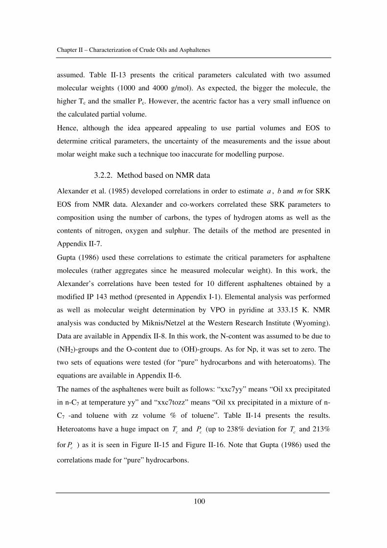
Chapter II – Characterization of Crude Oils and Asphaltenes
100
assumed. Table II-13 presents the critical parameters calculated with two assumed
molecular weights (1000 and 4000 g/mol). As expected, the bigger the molecule, the
higher Tc and the smaller Pc. However, the acentric factor has a very small influence on
the calculated partial volume.
Hence, although the idea appeared appealing to use partial volumes and EOS to
determine critical parameters, the uncertainty of the measurements and the issue about
molar weight make such a technique too inaccurate for modelling purpose.
3.2.2. Method based on NMR data
Alexander et al. (1985) developed correlations in order to estimate a , b and m for SRK
EOS from NMR data. Alexander and co-workers correlated these SRK parameters to
composition using the number of carbons, the types of hydrogen atoms as well as the
contents of nitrogen, oxygen and sulphur. The details of the method are presented in
Appendix II-7.
Gupta (1986) used these correlations to estimate the critical parameters for asphaltene
molecules (rather aggregates since he measured molecular weight). In this work, the
Alexander’s correlations have been tested for 10 different asphaltenes obtained by a
modified IP 143 method (presented in Appendix I-1). Elemental analysis was performed
as well as molecular weight determination by VPO in pyridine at 333.15 K. NMR
analysis was conducted by Miknis/Netzel at the Western Research Institute (Wyoming).
Data are available in Appendix II-8. In this work, the N-content was assumed to be due to
(NH2)-groups and the O-content due to (OH)-groups. As for Np, it was set to zero. The
two sets of equations were tested (for “pure” hydrocarbons and with heteroatoms). The
equations are available in Appendix II-6.
The names of the asphaltenes were built as follows: “xxc7yy” means “Oil xx precipitated
in n-C7 at temperature yy” and “xxc7tozz” means “Oil xx precipitated in a mixture of n-
C7 -and toluene with zz volume % of toluene”. Table II-14 presents the results.
Heteroatoms have a huge impact on cT and cP (up to 238% deviation for cT and 213%
for cP ) as it is seen in Figure II-15 and Figure II-16. Note that Gupta (1986) used the
correlations made for “pure” hydrocarbons.
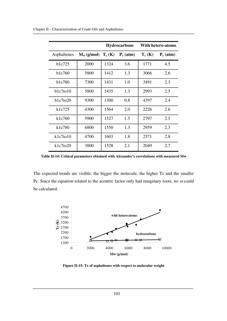
Chapter II – Characterization of Crude Oils and Asphaltenes
101
Hydrocarbons With hetero-atoms
Asphaltenes Mw (g/mol) Tc (K) Pc (atm) Tc (K) Pc (atm)
b1c725 2000 1324 3.6 1771 4.5
b1c760 5800 1412 1.3 3066 2.6
b1c780 7300 1431 1.0 3491 2.3
b1c7to10 5800 1435 1.3 2993 2.5
b1c7to20 9300 1300 0.8 4397 2.4
k1c725 4300 1564 2.0 2226 2.6
k1c760 5900 1527 1.5 2797 2.5
k1c780 6800 1550 1.3 2959 2.3
k1c7to10 4700 1603 1.8 2571 2.8
k1c7to20 3800 1528 2.1 2049 2.7
Table II-14: Critical parameters obtained with Alexander’s correlations with measured Mw
The expected trends are visible: the bigger the molecule, the higher Tc and the smaller
Pc. Since the equation related to the acentric factor only had imaginary roots, no ω could
be calculated.
12001700
2200270032003700
42004700
0 2000 4000 6000 8000 10000
Mw (g/mol)
Tc
(K)
with hetero-atoms
hydrocarbons
Figure II-15: Tc of asphaltenes with respect to molecular weight
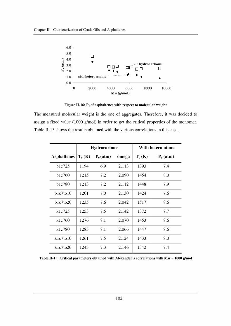
Chapter II – Characterization of Crude Oils and Asphaltenes
102
0.0
1.0
2.0
3.0
4.0
5.0
6.0
0 2000 4000 6000 8000 10000Mw (g/mol)
Pc
(atm
)hydrocarbons
with hetero atoms
Figure II-16: Pc of asphaltenes with respect to molecular weight
The measured molecular weight is the one of aggregates. Therefore, it was decided to
assign a fixed value (1000 g/mol) in order to get the critical properties of the monomer.
Table II-15 shows the results obtained with the various correlations in this case.
Hydrocarbons With hetero-atoms
Asphaltenes Tc (K) Pc (atm) omega Tc (K) Pc (atm)
b1c725 1194 6.9 2.113 1393 7.4
b1c760 1215 7.2 2.090 1454 8.0
b1c780 1213 7.2 2.112 1448 7.9
b1c7to10 1201 7.0 2.130 1424 7.6
b1c7to20 1235 7.6 2.042 1517 8.6
k1c725 1253 7.5 2.142 1372 7.7
k1c760 1276 8.1 2.070 1453 8.6
k1c780 1283 8.1 2.066 1447 8.6
k1c7to10 1261 7.5 2.124 1433 8.0
k1c7to20 1243 7.3 2.146 1342 7.4
Table II-15: Critical parameters obtained with Alexander’s correlations with Mw = 1000 g/mol
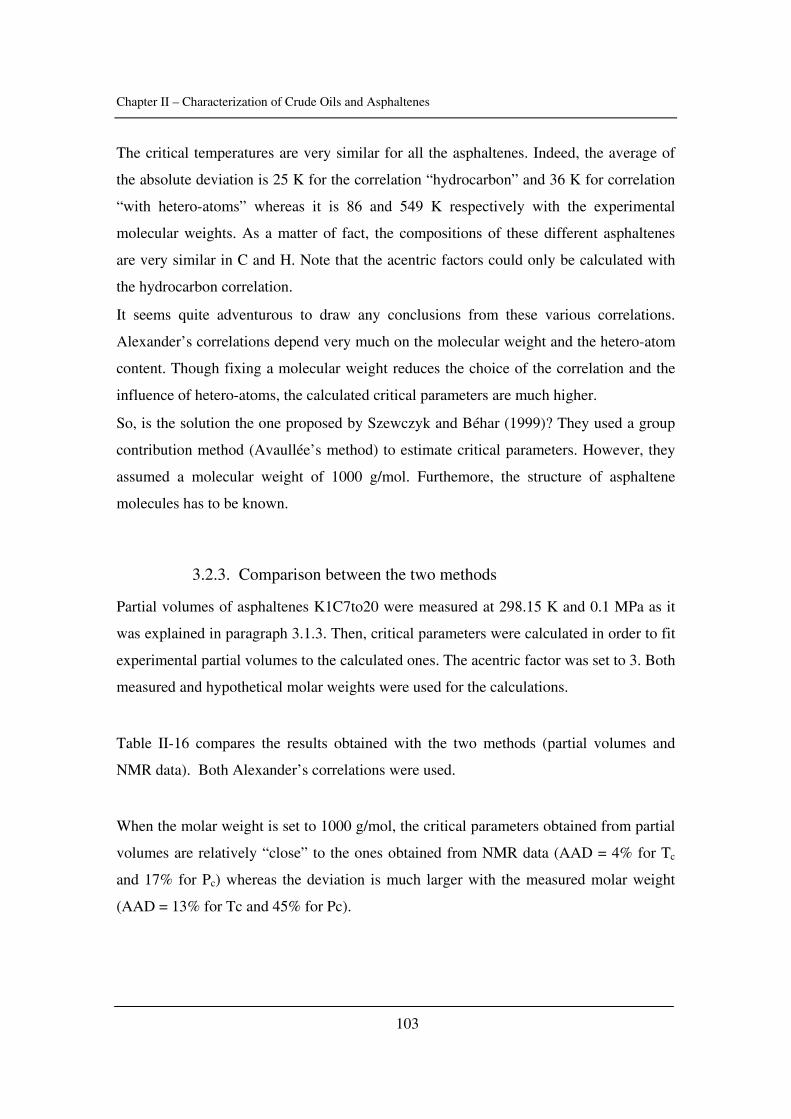
Chapter II – Characterization of Crude Oils and Asphaltenes
103
The critical temperatures are very similar for all the asphaltenes. Indeed, the average of
the absolute deviation is 25 K for the correlation “hydrocarbon” and 36 K for correlation
“with hetero-atoms” whereas it is 86 and 549 K respectively with the experimental
molecular weights. As a matter of fact, the compositions of these different asphaltenes
are very similar in C and H. Note that the acentric factors could only be calculated with
the hydrocarbon correlation.
It seems quite adventurous to draw any conclusions from these various correlations.
Alexander’s correlations depend very much on the molecular weight and the hetero-atom
content. Though fixing a molecular weight reduces the choice of the correlation and the
influence of hetero-atoms, the calculated critical parameters are much higher.
So, is the solution the one proposed by Szewczyk and Béhar (1999)? They used a group
contribution method (Avaullée’s method) to estimate critical parameters. However, they
assumed a molecular weight of 1000 g/mol. Furthemore, the structure of asphaltene
molecules has to be known.
3.2.3. Comparison between the two methods
Partial volumes of asphaltenes K1C7to20 were measured at 298.15 K and 0.1 MPa as it
was explained in paragraph 3.1.3. Then, critical parameters were calculated in order to fit
experimental partial volumes to the calculated ones. The acentric factor was set to 3. Both
measured and hypothetical molar weights were used for the calculations.
Table II-16 compares the results obtained with the two methods (partial volumes and
NMR data). Both Alexander’s correlations were used.
When the molar weight is set to 1000 g/mol, the critical parameters obtained from partial
volumes are relatively “close” to the ones obtained from NMR data (AAD = 4% for Tc
and 17% for Pc) whereas the deviation is much larger with the measured molar weight
(AAD = 13% for Tc and 45% for Pc).
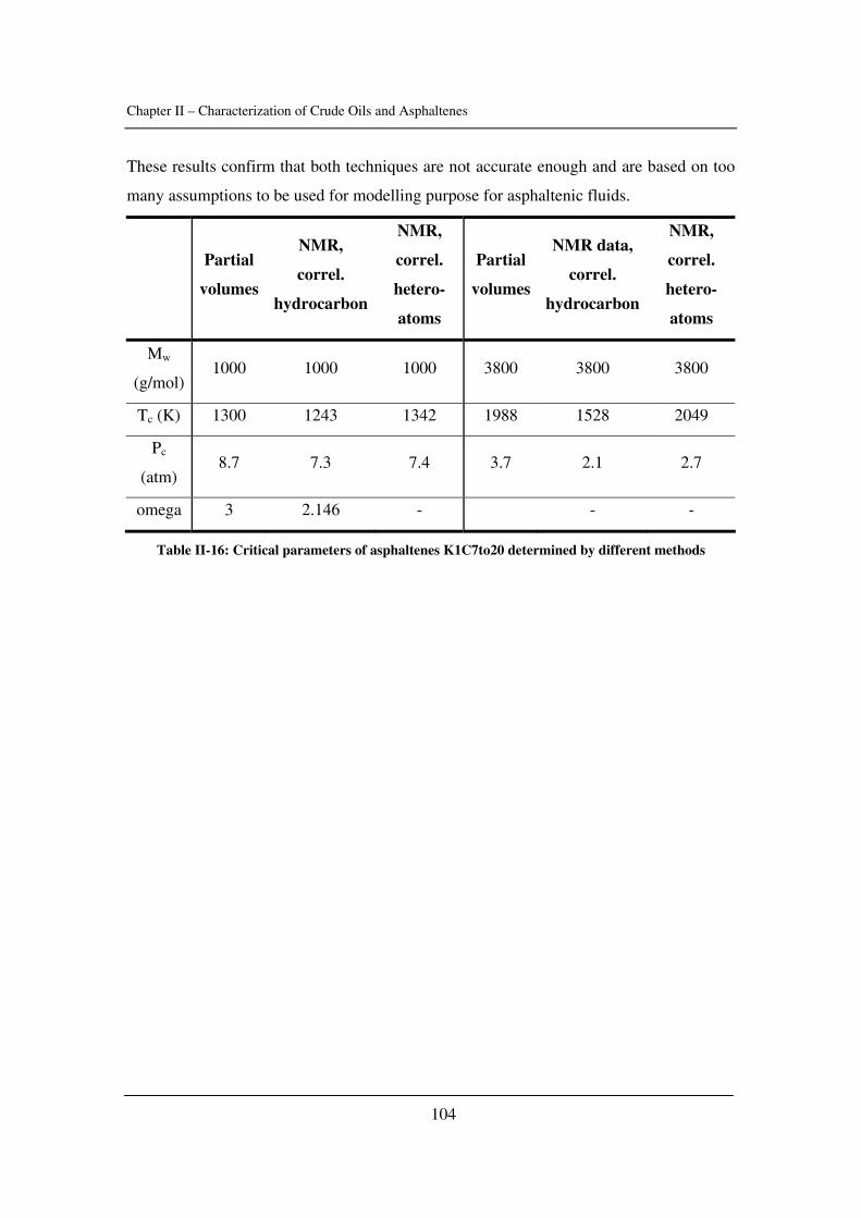
Chapter II – Characterization of Crude Oils and Asphaltenes
104
These results confirm that both techniques are not accurate enough and are based on too
many assumptions to be used for modelling purpose for asphaltenic fluids.
Partial
volumes
NMR,
correl.
hydrocarbon
NMR,
correl.
hetero-
atoms
Partial
volumes
NMR data,
correl.
hydrocarbon
NMR,
correl.
hetero-
atoms
Mw
(g/mol) 1000 1000 1000 3800 3800 3800
Tc (K) 1300 1243 1342 1988 1528 2049
Pc
(atm) 8.7 7.3 7.4 3.7 2.1 2.7
omega 3 2.146 - - -
Table II-16: Critical parameters of asphaltenes K1C7to20 determined by different methods
Chapter II – Characterization of Crude Oils and Asphaltenes
105
4. Conclusion
Solubility parameters are widely used but their definition is often up to the user. When
pressure and temperature are studied, cohesive energy should be defined as the residual
internal energy. Indeed, pressure strongly affects cohesive energy - contrary to the usual
belief – as it was checked for three pure compounds up to 100 MPa.
Internal pressure is an alternative to measure the solubility parameter of complex liquid
compounds and with respect to pressure and temperature. However, its determination is
not accurate enough to give proper results with modelling (1 MPa1/2). In addition,
hydrogen bonds are not taken into account by this physical property.
Solubility parameters of asphaltenes can be measured by various techniques but none of
them seem accurate enough. The method applied here for the first time to asphaltenes
gave results in agreement with another technique. However, the deviation (between 0.7
and 1.6 MPa1/2) is not compatible with modelling.
Critical parameters were also determined with two techniques: a new one (based on
molar volumes) and another one (based on NMR data). None of these methods give exact
enough critical properties.
Hence, the characterisation of crude oil and asphaltenes was investigated but the complex
and polydisperse nature of these systems induces large uncertainties in any technique
used. Are parameters related to asphaltenes bound to remain fitting parameters?
Chapter II – Characterization of Crude Oils and Asphaltenes
106
Literature Alexander G.L., Schwarz B.J., Prausnitz J.M., Phase Equilibria for high-boiling fossil-fuel distillates. 2. Correlation of equation of state constants with characterization data for phase equilibrium calculations, Ind. Eng. Chem. Fundam. (1985), 24, 311 – 315 Allen G., Gee G., Wislon G.J., Intermolecular forces and chain flexibility in polymers: internal pressures and cohesive energy densities of simple liquids, Polymer (1960), 456 – 466 Amoros J., Solana J.R., Vilar E., Behaviour of the internal pressure of liquids in accordance with variations in temperature, volume and cohesive energy density, Mat. Chem. Phys. (1984), 10, 6, 557 – 578 Andersen S.I., Flocculation onset titration of petroleum asphaltenes, Energ. Fuel. (1999), 13, 315 – 322 Bagley E.B., Nelson T.P., Scigliano J.M., Three dimensional solubility parameters and their relationship to internal measurements in polar and hydrogen bonding solvents, J. Paint Technol. (1971), 43, 35 – 42 Barbosa E.F.G., Sousa S.M.C., M.S.C.S. Santos, I.M.S. Lampreia, Partial molar volumes of linear hydrocarbons in methanol in the very dilute region. Intermolecular interactions. H-bond effects, Phys. Chem. Chem. Phys. (2001), 3, 556 – 561 Barton A.F.M., CRC Handbook of solubility parameters and other cohesion parameters; CRC Press, Inc., 1983 Barton A.F.M., CRC Handbook of solubility parameters and other cohesion parameters; CRC Press, Inc., 1991 Buckley J.S., Hirasaki G.J., Liu Y., Von Drasek S., Wang J.-X., Gill B.S., Asphaltene precipitation and solvent properties of crude oils, Pet. Sci. Technol.(1998), 16, 251 – 285 Cavett R.H., Physical Data for Distillation Calculations-Vapor-Liquid Equilibria, Proc., 27th API Meeting, San Francisco 351, 1962 Christiansen S.D., Properties of Asphaltenes, Master Thesis, Department of Chemical Engineering, Technical University of Denmark, February 1999 Chung F.T.H., Thermodynamic modelling for organic solid precipitation, SPE 24851 (1992), 869 – 878
Chapter II – Characterization of Crude Oils and Asphaltenes
107
Cibulka I., Hnedkovsky L., Liquid densities at elevated pressures of n-alkanes from C5 to C16. A critical evaluation of experimental data, J. Chem. Eng. Data (1996), 41, 657 – 668 Cibulka I., Takagi T., P-rho-T data of liquids: summarization and Evaluation. 5 – Aromatic hydrocarbons, J. Chem. Eng. Data (1999), 44, 411 - 429 Duong D., Determination of Solubility Parameters for Crude Oils, Master Thesis, Department of Chemical Engineering, Technical University of Denmark, Sept. 2004 Ensley K.E., Thermodynamics of asphalt intermolecular interactions and asphalt-aggregate interactions, in: T.F. Yen and G.V. Chilingarian (Ed), Asphaltenes and asphalts, 1. Developments in petroleum science, 40, 401 – 426, 1994 Fenistein D., Barré L., Broseta D., Espinat D., Livet A., Roux J.N., Scarsella M., Viscosimetric and neutron scattering study of asphaltene aggregates in mixed toluene/heptane solvents, Langmuir (1998), 14, 1013 – 1020 Gupta A.K., A model for asphaltene flocculation using an equation of state, Master Thesis, University of Calgary, Calgary, Canada, 1986 Hansen C.M., The three dimensional solubility parameter and solvent diffusion coefficient, Danish Technical Press, Copenhagen, 1967 Hildebrand J.H., Dymond J., Partial molal volumes in regular solutions, J. Chem. Phys. (1967), 46, 2, 624 – 626 Hildebrand J.H., Prausnitz J. M., Scott R.L., Regular and related solutions, Van Nostrand Reinhold Company, New-York, 1970 Hildebrand J.H., Scott R.L., The solubility of nonelectrolytes, Reinhold, New York, 1950
Hirschberg A., deJong L.N.J., Schipper B.A., Meijer J.G., Influence of temperature and Pressure on asphaltene flocculation, paper SPE 11202, SPEJ (1984) 283 – 293
Hoy K.L., New values of the solubility parameters from vapor pressure data, J. Paint. Technol.(1970), 42, 1, 76 – 118
Israelachvili J.N., Intermolecular and surface forces, 2nd edition, Academic Press (1992)
Kesler M.G., Lee B.I., Improve Predictions of Enthalpy of Fractions, Hydro. Proc. (1976), 55, 153
Chapter II – Characterization of Crude Oils and Asphaltenes
108
Lagourette B., Boned C., Saint-Guirons H., Xans P., Zhou H., Densimeter calibration method versus temperature and pressure, Meas, Sci. technol. (1992), 3, 699 - 703 Laux H., Löslichkeitsparameter und Verteiliugn von Erdölrückstands-Komponenten, Erdöl Erdgas Kohle (1992), 108, 5, 227 – 232 Lian L., Peptization studies of asphaltene and solubility parameter spectra, Fuel (1994), 73, 3, 423 – 428 Liron X., Cohen S., Densitometric determination of the solubility parameter and molal volume of compounds of medicinal relevance, J. Pharm. Sci. (1983), 72, 499 - 504 Lyckman E.W., Eckert C.A., Prausnitz J.M., Generalized liquid volumes and solubility parameters for regular solution application, Chem. Eng. Sci. (1965), 20, 703 – 706
Maloney D.P., Prausnitz J.M., Thermodynamic properties of liquid polyethylene, Journal of applied polymer science (1974), 18, 2703 - 2710 Marrero J., Gani R., Group-contribution based estimation of pure component properties, Fluid Phase Equilibr. (2001), 183-184, 183-208 Michelsen M.L., Mollerup J.M., Thermodynamic models: fundamentals and computational aspects, Tie-Line Publications, Holte, 2004 Montel F., Petroleum Thermodynamics, Notes, Total, 2004 Moore W.J., Physical Chemistry, 3rd edition, Longmans, London, 1959, pp 423-424 Mutelet F., Ekulu G., Solimando R., Rogalski, Solubility parameters of crude oils and asphaltenes, Energ. Fuel. (2004), 18, 667 - 673 Nghiem L.X., Hassam M.S., Nutakki R., George A.E.D., Efficient modelling of asphaltene precipitation, SPE 26642 (1993) Nokay R., Estimate Petrochemical Properties, Chem. Eng. (1959), 147 Null H.R., Palmer D.A., Predicting Phase Equilibria, Chem.Eng.Prog. (1969), 65, 47 – 51 Perry, R.H., Green, D.W., Maloney, J.O., Perry’s chemical engineers’ handbook (7th edition), McGraw-Hill, New-York, 1997 Randzio S.L., Scanning calorimeters controlled by an independent thermodynamic variable: definitions and some metrological problems, Thermochim. Acta (1985), 89, 215 – 241
Chapter II – Characterization of Crude Oils and Asphaltenes
109
Riazi M.R., Daubert, T.E., Simplify Property Predictions, Hydro. Proc. (1980), 115 Sun T.F., Bominaar S.A.R.C., Ten Seldam C.A., Biswas S.N., Evaluation of the thermophysical properties of toluene and n-heptane from 180 to 320 K and up to 260 Mpa from speed-of-sound data, Berich. Bunsen Gesell. (1991), 95, 696 – 704 Sun T.F., Kortbeek P.J., Trappeniers N.J., Biswas S.N., Acoustic and thermodynamic properties of benzene and cyclohexane as a function of pressure and temperature, Phys. Chem. Liq. (1987), 16, 163 – 178 Szewczyk V., Behar E., Compositional model for predicting asphaltenes flocculation, Fluid Phase Equilibr. (1999), 158, 459 – 469 Taravillo M., Castro S., Garcia Baonza V., Caceres M., Nunez J., Thermophysical properties of liquid m-xylene at high pressures, Chem. Soc. Faraday. Trans. (1994), 90, 1217 – 1221 Torcal-Garcia V., Asphaltene phase stability after hydrotreatment and heat treatment of heavy feedstocks, Master Thesis, Department of Chemical Engineering, Technical University of Denmark, 2004 Twu C.H., An internally consistent correlation for predicting the critical properties and molecular weights of petroleum and coal-tar liquids, Fluid Phase Equilibr. (1984), 137 – 150 Utracki L.A., Simha R., Statistical thermodynamics predictions of the solubility parameter, Polym. Int. (2004), 53, 279 – 286 Verdier S., Andersen S.I., Internal pressure and solubility parameter as a function of pressure, Fluid Phase Equilibr. (2005), 231, 125–137 Verdier S., Duong D., Andersen S.I., Experimental determination of solubility parameters of oils as function of pressure, Energ. Fuel. (2005), 19, 1225 - 1229 Wang J.X., Buckley J.S., A two-component solubility model of the onset of asphaltene flocculation in crude oils, Energ. Fuel. (2001), 15, 1004 – 1012 Weast R.C., Selby S.M., Handbook of chemistry and physics, 47th edition, The Chemical Rubber Co., Cleveland, 1966 Whitson C.H., Brulé M.R., Phase Behaviour, SPE Monograph, Vol. 20, Richardson, Texas, 2000
Chapter II – Characterization of Crude Oils and Asphaltenes
110
Won K.W., Thermodynamics for solid solution-liquid-vapor equilibria: wax phase formation from heavy hydrocarbons mixtures, Fluid Phase Equilibr. (1986), 30, 265 – 279 Yarranton H.W., Masliyah J.H., Molar mass distribution and solubility modeling of asphaltenes, AIChE (1996), 42, 12, 3533 - 3543 Zhou H., Thomas F.B., Moore R.G., Modelling of solid precipitation from reservoir fluid, J.C.P.T. (1996), 35, 10, 37 - 45

Chapter II – Characterization of Crude Oils and Asphaltenes
111
List of symbols
Latin letters
a Attractive term of a cubic EOS
b Co-volume
B Coefficient of the modified Tait equation
C Coefficient of the modified Tait equation
CED Cohesive Energy Density
E Cohesive energy
H Enthalpy
m Temperature dependence of the solubility parameter
n ratio between internal pressure and the cohesive energy density
P Pressure
R Gas constant
RI Refractive index
T Temperature
U Internal energy
V Molar volume
Greek letters
Pα Isobaric thermal expansivity
δ Solubility parameter
Tκ Isothermal compressibility
π Internal pressure
ρ Density
ω Acentric factor

Chapter II – Characterization of Crude Oils and Asphaltenes
112
Subscripts and Superscripts
A Attractive
c Critical
d Dispersion
h Hydrogen bonding
liq Liquid
p Polar
R Repulsive
r Residual
sat Saturation
v Volume-dependent
vap Vapour
0 Reference
Chapter III – Asphaltene Stability and Gas Injection
113
Chapter III
Asphaltene Stability and Gas Injection
Chapter III – Asphaltene Stability and Gas Injection
114
Table of Contents
1. Influence of pressure and temperature on asphaltene stability ....................... 116
1.1. Temperature and Asphaltene Precipitation..................................................... 116
1.2. Pressure and Asphaltene Precipitation............................................................ 118
1.3. Asphaltene Phase Envelopes........................................................................... 119
1.4. Le Châtelier’s principle................................................................................... 120
2. The Onset Determination ..................................................................................... 123
2.1. Determination of the onset of precipitation .................................................... 123
2.2. Determination of the onset of flocculation ..................................................... 125
2.3. Possible uncertainties...................................................................................... 127
3. Measurement of APE of recombined oil ............................................................. 129
3.1. Sampling and recombining method ................................................................ 129
3.2. Experimental set-up ........................................................................................ 130
3.3. Experimental procedure .................................................................................. 133
3.4. Influence of carbon dioxide ............................................................................ 134
3.5. Influence of methane....................................................................................... 138
3.6. Conclusions..................................................................................................... 140
3.7. Unanswered issues and future work ............................................................... 141
4. Conclusion ............................................................................................................. 143
Literature....................................................................................................................... 144
Chapter III – Asphaltene Stability and Gas Injection
115
What is the influence of pressure and temperature on asphaltene stability? Does
temperature equally affect precipitation induced by n-heptane, 2CO or methane? Are
there factors influencing reversibility? How can the onset be accurately determined?
First, the influence of pressure and temperature as it is reported in the literature will be
given. Then, the different techniques used to determine asphaltene precipitation and
flocculation will be briefly described. Finally, the experiments carried out with a novel
experimental set-up developed at the University of Pau will be presented. The effect of
pressure, temperature, gas nature and composition will be investigated for two crude oils.
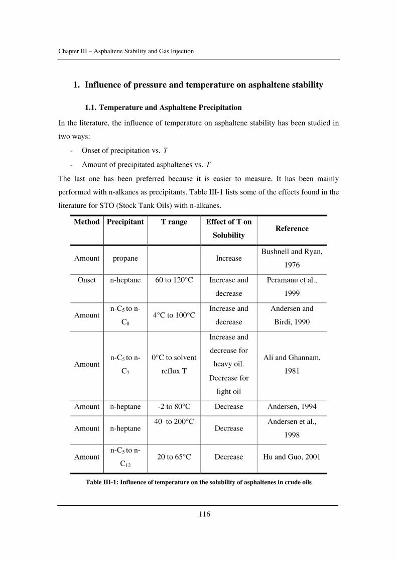
Chapter III – Asphaltene Stability and Gas Injection
116
1. Influence of pressure and temperature on asphaltene stability
1.1. Temperature and Asphaltene Precipitation
In the literature, the influence of temperature on asphaltene stability has been studied in
two ways:
- Onset of precipitation vs. T
- Amount of precipitated asphaltenes vs. T
The last one has been preferred because it is easier to measure. It has been mainly
performed with n-alkanes as precipitants. Table III-1 lists some of the effects found in the
literature for STO (Stock Tank Oils) with n-alkanes.
Method Precipitant T range Effect of T on
Solubility Reference
Amount propane Increase Bushnell and Ryan,
1976
Onset n-heptane 60 to 120°C Increase and
decrease
Peramanu et al.,
1999
Amount n-C5 to n-
C8 4°C to 100°C
Increase and
decrease
Andersen and
Birdi, 1990
Amount n-C5 to n-
C7
0°C to solvent
reflux T
Increase and
decrease for
heavy oil.
Decrease for
light oil
Ali and Ghannam,
1981
Amount n-heptane -2 to 80°C Decrease Andersen, 1994
Amount n-heptane 40 to 200°C
Decrease Andersen et al.,
1998
Amount n-C5 to n-
C12 20 to 65°C Decrease Hu and Guo, 2001
Table III-1: Influence of temperature on the solubility of asphaltenes in crude oils
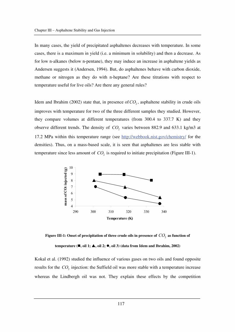
Chapter III – Asphaltene Stability and Gas Injection
117
In many cases, the yield of precipitated asphaltenes decreases with temperature. In some
cases, there is a maximum in yield (i.e. a minimum in solubility) and then a decrease. As
for low n-alkanes (below n-pentane), they may induce an increase in asphaltene yields as
Andersen suggests it (Andersen, 1994). But, do asphaltenes behave with carbon dioxide,
methane or nitrogen as they do with n-heptane? Are these titrations with respect to
temperature useful for live oils? Are there any general rules?
Idem and Ibrahim (2002) state that, in presence of 2CO , asphaltene stability in crude oils
improves with temperature for two of the three different samples they studied. However,
they compare volumes at different temperatures (from 300.4 to 337.7 K) and they
observe different trends. The density of 2CO varies between 882.9 and 633.1 kg/m3 at
17.2 MPa within this temperature range (see http://webbook.nist.gov/chemistry/ for the
densities). Thus, on a mass-based scale, it is seen that asphaltenes are less stable with
temperature since less amount of 2CO is required to initiate precipitation (Figure III-1).
4
5
6
7
8
9
10
290 300 310 320 330 340
Temperature (K)
mas
s of C
O2 i
njec
ted
(g)
Figure III-1: Onset of precipitation of three crude oils in presence of 2CO as function of
temperature ( , oil 1; , oil 2; , oil 3) (data from Idem and Ibrahim, 2002)
Kokal et al. (1992) studied the influence of various gases on two oils and found opposite
results for the 2CO injection: the Suffield oil was more stable with a temperature increase
whereas the Lindbergh oil was not. They explain these effects by the competition
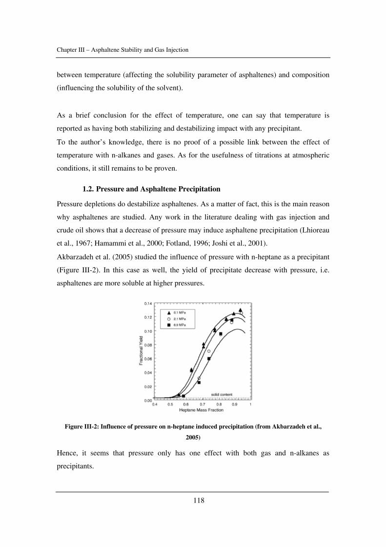
Chapter III – Asphaltene Stability and Gas Injection
118
between temperature (affecting the solubility parameter of asphaltenes) and composition
(influencing the solubility of the solvent).
As a brief conclusion for the effect of temperature, one can say that temperature is
reported as having both stabilizing and destabilizing impact with any precipitant.
To the author’s knowledge, there is no proof of a possible link between the effect of
temperature with n-alkanes and gases. As for the usefulness of titrations at atmospheric
conditions, it still remains to be proven.
1.2. Pressure and Asphaltene Precipitation
Pressure depletions do destabilize asphaltenes. As a matter of fact, this is the main reason
why asphaltenes are studied. Any work in the literature dealing with gas injection and
crude oil shows that a decrease of pressure may induce asphaltene precipitation (Lhioreau
et al., 1967; Hamammi et al., 2000; Fotland, 1996; Joshi et al., 2001).
Akbarzadeh et al. (2005) studied the influence of pressure with n-heptane as a precipitant
(Figure III-2). In this case as well, the yield of precipitate decrease with pressure, i.e.
asphaltenes are more soluble at higher pressures.
Figure III-2: Influence of pressure on n-heptane induced precipitation (from Akbarzadeh et al.,
2005)
Hence, it seems that pressure only has one effect with both gas and n-alkanes as
precipitants.
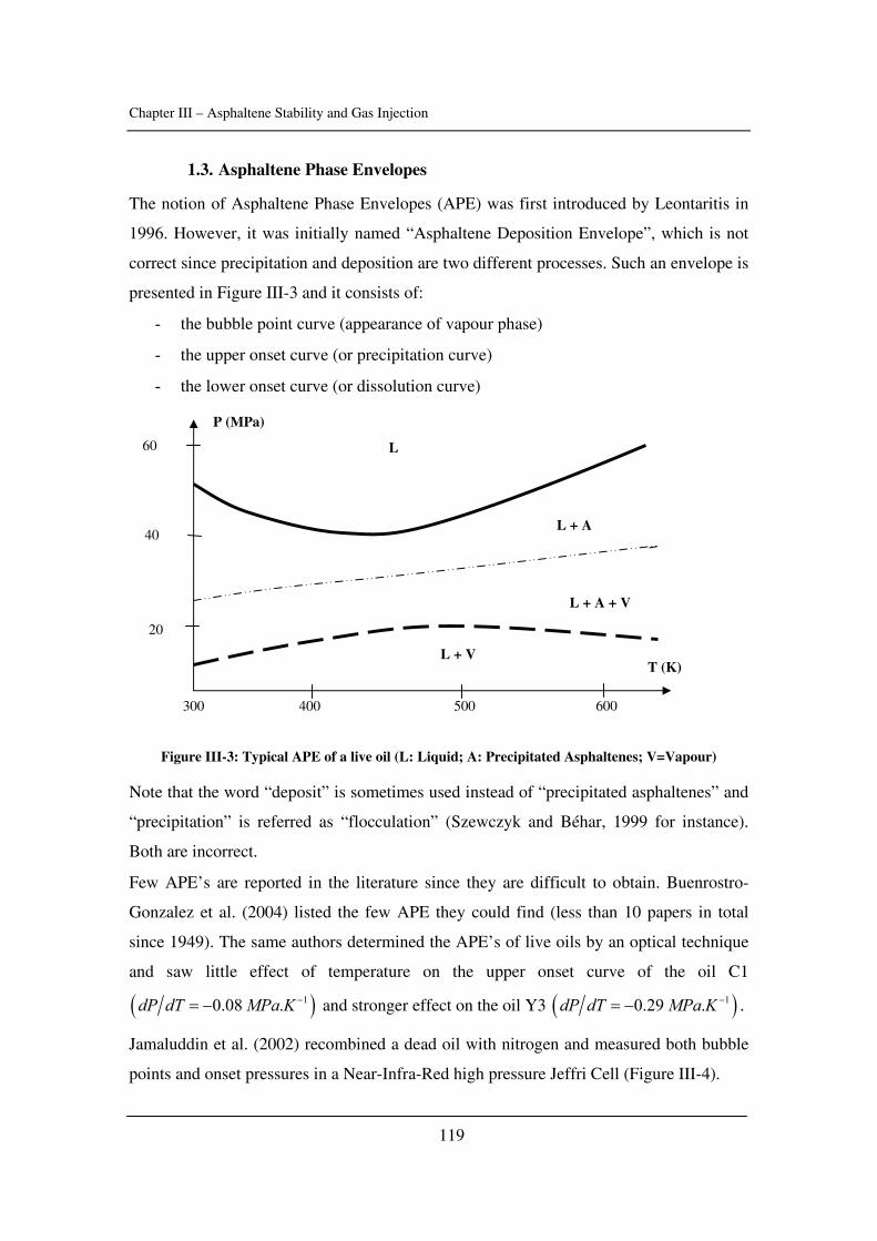
Chapter III – Asphaltene Stability and Gas Injection
119
1.3. Asphaltene Phase Envelopes
The notion of Asphaltene Phase Envelopes (APE) was first introduced by Leontaritis in
1996. However, it was initially named “Asphaltene Deposition Envelope”, which is not
correct since precipitation and deposition are two different processes. Such an envelope is
presented in Figure III-3 and it consists of:
- the bubble point curve (appearance of vapour phase)
- the upper onset curve (or precipitation curve)
- the lower onset curve (or dissolution curve)
Figure III-3: Typical APE of a live oil (L: Liquid; A: Precipitated Asphaltenes; V=Vapour)
Note that the word “deposit” is sometimes used instead of “precipitated asphaltenes” and
“precipitation” is referred as “flocculation” (Szewczyk and Béhar, 1999 for instance).
Both are incorrect.
Few APE’s are reported in the literature since they are difficult to obtain. Buenrostro-
Gonzalez et al. (2004) listed the few APE they could find (less than 10 papers in total
since 1949). The same authors determined the APE’s of live oils by an optical technique
and saw little effect of temperature on the upper onset curve of the oil C1
( )10.08 .dP dT MPa K −= − and stronger effect on the oil Y3 ( )10.29 .dP dT MPa K −= − .
Jamaluddin et al. (2002) recombined a dead oil with nitrogen and measured both bubble
points and onset pressures in a Near-Infra-Red high pressure Jeffri Cell (Figure III-4).
P (MPa)
20
40
60
T (K)
300 400 500 600
L
L + A
L + A + V
L + V
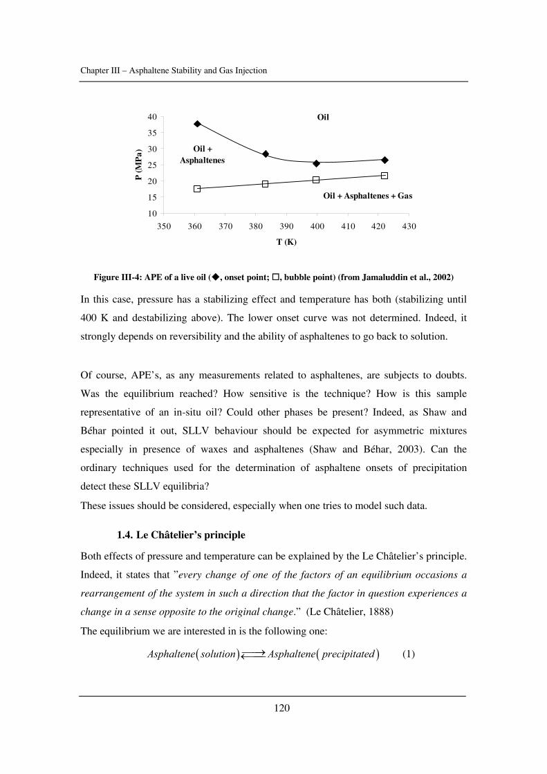
Chapter III – Asphaltene Stability and Gas Injection
120
10
15
20
25
30
35
40
350 360 370 380 390 400 410 420 430
T (K)
P (M
Pa)
Oil
Oil + Asphaltenes
Oil + Asphaltenes + Gas
Figure III-4: APE of a live oil ( , onset point; , bubble point) (from Jamaluddin et al., 2002)
In this case, pressure has a stabilizing effect and temperature has both (stabilizing until
400 K and destabilizing above). The lower onset curve was not determined. Indeed, it
strongly depends on reversibility and the ability of asphaltenes to go back to solution.
Of course, APE’s, as any measurements related to asphaltenes, are subjects to doubts.
Was the equilibrium reached? How sensitive is the technique? How is this sample
representative of an in-situ oil? Could other phases be present? Indeed, as Shaw and
Béhar pointed it out, SLLV behaviour should be expected for asymmetric mixtures
especially in presence of waxes and asphaltenes (Shaw and Béhar, 2003). Can the
ordinary techniques used for the determination of asphaltene onsets of precipitation
detect these SLLV equilibria?
These issues should be considered, especially when one tries to model such data.
1.4. Le Châtelier’s principle
Both effects of pressure and temperature can be explained by the Le Châtelier’s principle.
Indeed, it states that ”every change of one of the factors of an equilibrium occasions a
rearrangement of the system in such a direction that the factor in question experiences a
change in a sense opposite to the original change.” (Le Châtelier, 1888)
The equilibrium we are interested in is the following one:
( ) ( )Asphaltene solution Asphaltene precipitated⎯⎯→←⎯⎯ (1)
Chapter III – Asphaltene Stability and Gas Injection
121
Andersen and Speight (1999) listed two other reactions:
- the aggregation:
i l i lAsphaltenes Asphaltenes Asphaltenes ++ (2)
- the interaction with the resins:
resins resinsAsphaltenes Asphaltenes+ − (3)
Aggregation only takes place at low concentration as it was said in chapter 1, paragraph
1.4.1. Hence, equilibrium (2) can be neglected since the onset conditions are investigated
here. As for the interactions with resins, they can be seen as part of the asphaltene
continuum.
- The effect of pressure
If pressure is increased, the position of equilibrium will move so that the pressure is
reduced again, i.e. the number of molecules decreases or the volume is reduced.
Experimentally, it is seen that solubility of asphaltenes in oil increases with increasing
pressure. Thus, it means that the system decreases its volume when pressure is increased,
i.e. the volume of the two-phase region is larger than the one of the one-phase region. To
the authors’ knowledge, there is no experimental evidence of a gain in volume during
precipitation in the open literature except one recent work relating a decrease in a reduced
density with precipitation (Ekulu et al., 2004). The authors plotted the density of (crude
oil + solvent+ flocculant) – density (deasphalted oil + solvent + precipitant) as function
of the precipitant content. The break corresponds to asphaltene flocculation, as an optical
method confirmed it. In addition, as it is explained in Chapter 4, paragraph 3.3, a gain in
volume was observed on a recombined oil after precipitation.
Furthermore, by means of various equations of state (EOS) (CPA in Knudsen, 2001 and
SAFT in Christensen et al., 2005), an increase of 10 cm3 per mole at 400 K was
calculated between the onset and the bubble point as follows:
11 phase
RTZvP
= Eq III-1
( )2 phases oil oil asphaltene asphalteneRTv x Z x ZP
= + Eq III-2
Chapter III – Asphaltene Stability and Gas Injection
122
where v is the molar volume, T the temperature, P the pressure, x the mole fraction and
Z the compressibility factor.
The difference 2 1phases phasesv v− gives the volumetric variations due to asphaltene
precipitation and the increase due to asphaltene is approximately 50% of the total change.
Similar calculations with a cubic EOS are presented in Chapter 5, paragraph 2.4. It is
concluded that, for 1 mole of a system (99% oil+1% asphaltenes) with average densities
and molecular weights, the volume change due to the asphaltene phase itself is less than
0.05 cm3, which is very little to be detected.
Hence, pressure seems to stabilize asphaltenes and precipitation seems to be followed by
an increase in volume, as the Le Châtelier’s principle predicted it.
- The effect of temperature
If temperature is increased, the Le Châtelier’s principle states that the position of
equilibrium (1) will move so that the temperature is reduced again. If the reaction is
exothermic, the equilibrium will go to the left side when temperature is increased, i.e.
asphaltenes will be more soluble. If not, the asphaltenes will be less soluble. As it was
said previously, both stabilizing and destabilizing effects are found in the literature.
Could it be that some asphaltene precipitations are exothermic and some others
endothermic? Is it due to the solvent properties or to the asphaltenes themselves?
The calorimetric aspect of precipitation is detailed in Chapter 4. In the literature,
precipitation induced by n-alkanes is reported to be endothermic whereas it is exothermic
for live oils and by pressure depletion. Our work presented in chapter 4 confirmed the
second result but not the first one. So far, there are not enough experimental evidences to
relate the exo- or endothermy of asphaltene precipitation to the impact of temperature on
stability.
The Le Châtelier’s principle can also be explained by equations as shown in Appendix 3-
1 (influence of pressure and temperature on the equilibrium constant). The effect of
temperature on the equilibrium is related to the heat of reaction and the effect of pressure
to the molar volume of asphaltene in the different phases.
Chapter III – Asphaltene Stability and Gas Injection
123
2. The Onset Determination
As it was said in Chapter 1, paragraph 1.6.2, almost all the possible techniques have been
used to detect asphaltene precipitation: microscopic examination, optical transmission
and light-scattering, conductivity measurements, viscosimetry, particle size analysis,
fluorescence spectroscopy, density measurements or acoustic methods. Several questions
raises: do they determine the onset of precipitation or flocculation? How accurate are
they? Can they be applied to live oil systems? Could they eventually determine SLLV
phase behaviour?
This paragraph aims at studying these different techniques and list their advantages and
drawbacks. A closer look will be given to filtration since this technique has been applied
in this work.
2.1. Determination of the onset of precipitation
Few methods determine onsets of precipitation: viscosity measurements (El-Mohamed
et al., 1988; Escobedo and Mansoori, 1994), filtration techniques (Leontaritis et al.,
1994), methods based on heat transfer (Clarke and Pruden, 1997), electrical
conductivity (Fotland et al., 1993) and density-based procedures (Ekulu et al., 2004).
Indeed, asphaltene precipitation is the formation of a solid-like phase and hence the
mentioned techniques render the appearance of such a phase. On the contrary,
flocculation is a state of aggregation and asphaltenes are still in solution.
- Viscosity
El-Mohamed et al. (1988) studied the effect of viscosity next to the onset point with a
horizontal Ostwald viscometer. The asphaltenic solutions shifted from Newtonian
behaviour to non-Newtonian across the onset.
Escobedo and Mansoori (1994) extended this method to crude oils but still at room
conditions. Note that they claimed developing a new technique.
- Heat Transfer
Clarke and Pruden (1997) developed an interesting technique based on heat transfer
through a precipitate layer. N-heptane induced precipitation was investigated at room
conditions. It is likely that an important quantity of precipitate is formed before detecting
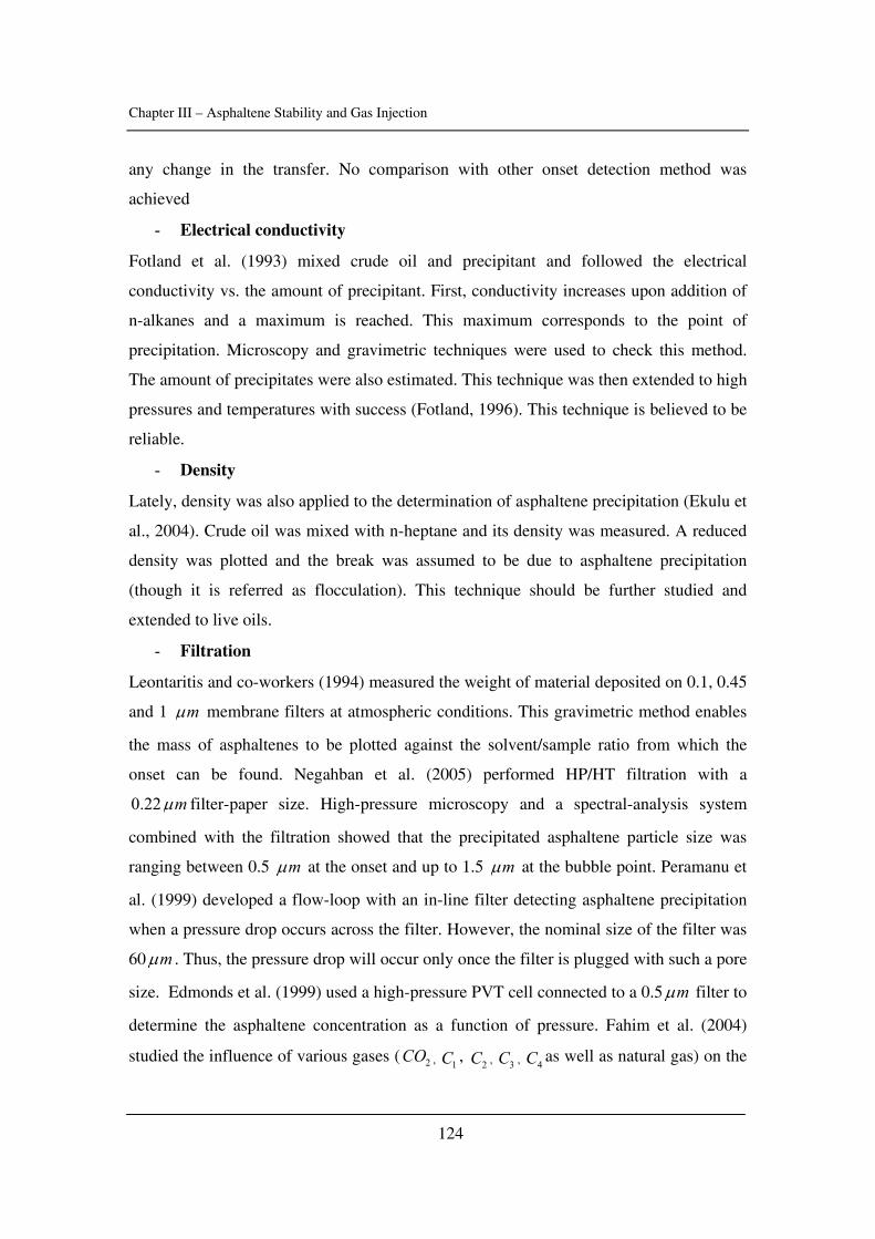
Chapter III – Asphaltene Stability and Gas Injection
124
any change in the transfer. No comparison with other onset detection method was
achieved
- Electrical conductivity
Fotland et al. (1993) mixed crude oil and precipitant and followed the electrical
conductivity vs. the amount of precipitant. First, conductivity increases upon addition of
n-alkanes and a maximum is reached. This maximum corresponds to the point of
precipitation. Microscopy and gravimetric techniques were used to check this method.
The amount of precipitates were also estimated. This technique was then extended to high
pressures and temperatures with success (Fotland, 1996). This technique is believed to be
reliable.
- Density
Lately, density was also applied to the determination of asphaltene precipitation (Ekulu et
al., 2004). Crude oil was mixed with n-heptane and its density was measured. A reduced
density was plotted and the break was assumed to be due to asphaltene precipitation
(though it is referred as flocculation). This technique should be further studied and
extended to live oils.
- Filtration
Leontaritis and co-workers (1994) measured the weight of material deposited on 0.1, 0.45
and 1 mμ membrane filters at atmospheric conditions. This gravimetric method enables
the mass of asphaltenes to be plotted against the solvent/sample ratio from which the
onset can be found. Negahban et al. (2005) performed HP/HT filtration with a
0.22 mμ filter-paper size. High-pressure microscopy and a spectral-analysis system
combined with the filtration showed that the precipitated asphaltene particle size was
ranging between 0.5 mμ at the onset and up to 1.5 mμ at the bubble point. Peramanu et
al. (1999) developed a flow-loop with an in-line filter detecting asphaltene precipitation
when a pressure drop occurs across the filter. However, the nominal size of the filter was
60 mμ . Thus, the pressure drop will occur only once the filter is plugged with such a pore
size. Edmonds et al. (1999) used a high-pressure PVT cell connected to a 0.5 mμ filter to
determine the asphaltene concentration as a function of pressure. Fahim et al. (2004)
studied the influence of various gases ( 2CO , 1C , 2C , 3C , 4C as well as natural gas) on the
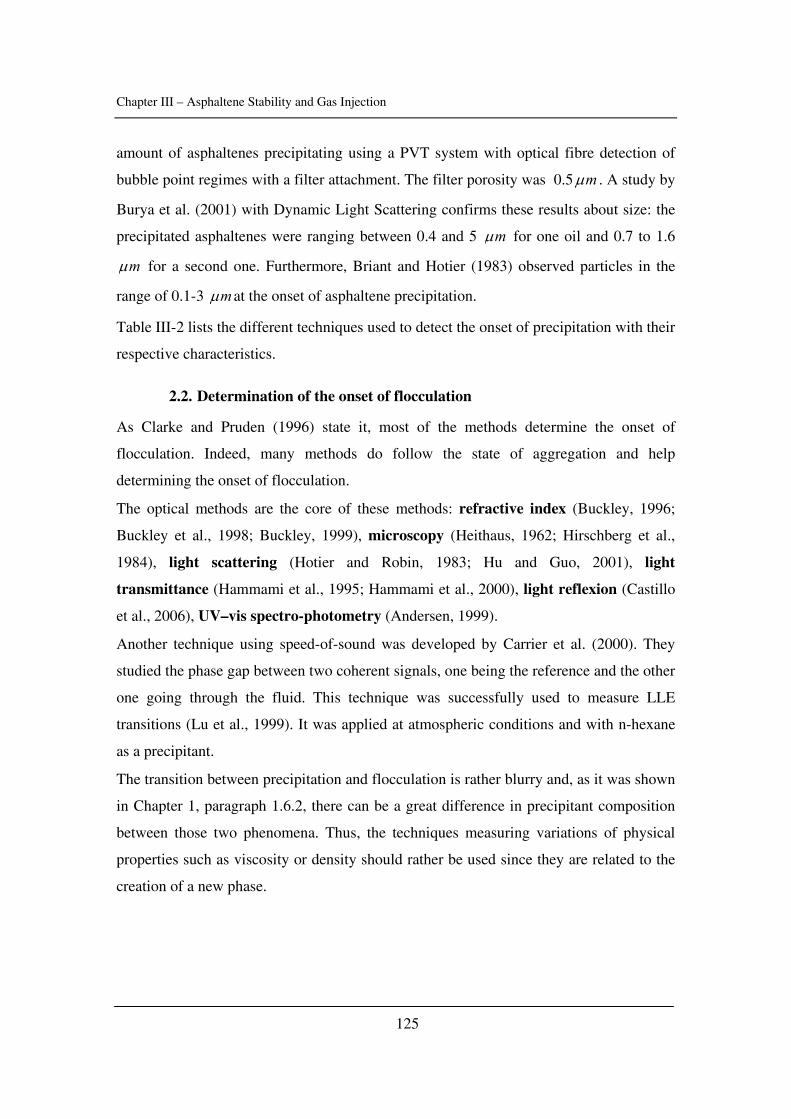
Chapter III – Asphaltene Stability and Gas Injection
125
amount of asphaltenes precipitating using a PVT system with optical fibre detection of
bubble point regimes with a filter attachment. The filter porosity was 0.5 mμ . A study by
Burya et al. (2001) with Dynamic Light Scattering confirms these results about size: the
precipitated asphaltenes were ranging between 0.4 and 5 mμ for one oil and 0.7 to 1.6
mμ for a second one. Furthermore, Briant and Hotier (1983) observed particles in the
range of 0.1-3 mμ at the onset of asphaltene precipitation.
Table III-2 lists the different techniques used to detect the onset of precipitation with their
respective characteristics.
2.2. Determination of the onset of flocculation
As Clarke and Pruden (1996) state it, most of the methods determine the onset of
flocculation. Indeed, many methods do follow the state of aggregation and help
determining the onset of flocculation.
The optical methods are the core of these methods: refractive index (Buckley, 1996;
Buckley et al., 1998; Buckley, 1999), microscopy (Heithaus, 1962; Hirschberg et al.,
1984), light scattering (Hotier and Robin, 1983; Hu and Guo, 2001), light
transmittance (Hammami et al., 1995; Hammami et al., 2000), light reflexion (Castillo
et al., 2006), UV–vis spectro-photometry (Andersen, 1999).
Another technique using speed-of-sound was developed by Carrier et al. (2000). They
studied the phase gap between two coherent signals, one being the reference and the other
one going through the fluid. This technique was successfully used to measure LLE
transitions (Lu et al., 1999). It was applied at atmospheric conditions and with n-hexane
as a precipitant.
The transition between precipitation and flocculation is rather blurry and, as it was shown
in Chapter 1, paragraph 1.6.2, there can be a great difference in precipitant composition
between those two phenomena. Thus, the techniques measuring variations of physical
properties such as viscosity or density should rather be used since they are related to the
creation of a new phase.

Cha
pter
III
– A
spha
ltene
Sta
bilit
y an
d G
as I
njec
tion
12
6
Tec
hniq
ue
Syst
em
Con
diti
ons
Adv
anta
ges
Dra
wba
cks
Ref
eren
ce
Vis
cosi
ty
Asp
halt
ene
solu
tion
s 29
3 K
, 0.1
MPa
Fa
st
Lim
ited
wor
king
con
ditio
ns
Not
test
ed w
ith
crud
e oi
ls
Stro
ngly
tim
e-de
pend
ent
El-
Moh
amed
et
al.,
1988
Hea
t Tra
nsfe
r C
rude
oil
30
1 K
, 0.1
MPa
Tes
ted
wit
h n-
hept
ane
Not
com
pare
d to
oth
er o
nset
te
chni
ques
Im
port
ant p
reci
pita
te n
eces
sary
to
det
ect a
cha
nge
Cla
rke
and
Prud
en, 1
997
Ele
ctri
cal
cond
ucti
vity
C
rude
oil
U
ntil
70
MPa
and
39
3 K
Rel
iabl
e W
ide
wor
king
co
ndit
ions
C
heck
ed w
ith
othe
r m
etho
ds
Fo
tlan
d et
al.,
19
93
Fotl
and,
199
6
Den
sity
C
rude
oil
R
oom
con
ditio
ns
Eas
y T
o be
ext
ende
d an
d ch
ecke
d L
imit
ed c
ondi
tion
s E
kulu
et a
l., 2
004
Filt
ratio
n C
rude
oil
H
P/H
T
Rel
iabl
e S
ize
of p
reci
pita
ted
asph
alte
nes
is a
ssum
ed
Neg
ahba
n et
al.
(200
5)
Tab
le I
II-2
: E
xam
ples
of
tech
niqu
es u
sed
for
the
dete
rmin
atio
n of
the
ons
et o
f pr
ecip
itat
ion
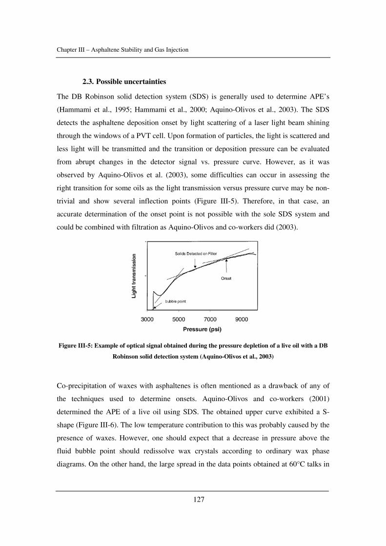
Chapter III – Asphaltene Stability and Gas Injection
127
2.3. Possible uncertainties
The DB Robinson solid detection system (SDS) is generally used to determine APE’s
(Hammami et al., 1995; Hammami et al., 2000; Aquino-Olivos et al., 2003). The SDS
detects the asphaltene deposition onset by light scattering of a laser light beam shining
through the windows of a PVT cell. Upon formation of particles, the light is scattered and
less light will be transmitted and the transition or deposition pressure can be evaluated
from abrupt changes in the detector signal vs. pressure curve. However, as it was
observed by Aquino-Olivos et al. (2003), some difficulties can occur in assessing the
right transition for some oils as the light transmission versus pressure curve may be non-
trivial and show several inflection points (Figure III-5). Therefore, in that case, an
accurate determination of the onset point is not possible with the sole SDS system and
could be combined with filtration as Aquino-Olivos and co-workers did (2003).
Figure III-5: Example of optical signal obtained during the pressure depletion of a live oil with a DB
Robinson solid detection system (Aquino-Olivos et al., 2003)
Co-precipitation of waxes with asphaltenes is often mentioned as a drawback of any of
the techniques used to determine onsets. Aquino-Olivos and co-workers (2001)
determined the APE of a live oil using SDS. The obtained upper curve exhibited a S-
shape (Figure III-6). The low temperature contribution to this was probably caused by the
presence of waxes. However, one should expect that a decrease in pressure above the
fluid bubble point should redissolve wax crystals according to ordinary wax phase
diagrams. On the other hand, the large spread in the data points obtained at 60°C talks in
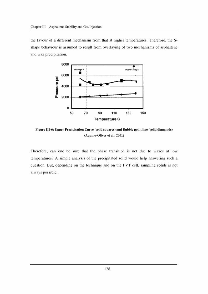
Chapter III – Asphaltene Stability and Gas Injection
128
the favour of a different mechanism from that at higher temperatures. Therefore, the S-
shape behaviour is assumed to result from overlaying of two mechanisms of asphaltene
and wax precipitation.
Figure III-6: Upper Precipitation Curve (solid squares) and Bubble point line (solid diamonds)
(Aquino-Olivos et al., 2001)
Therefore, can one be sure that the phase transition is not due to waxes at low
temperatures? A simple analysis of the precipitated solid would help answering such a
question. But, depending on the technique and on the PVT cell, sampling solids is not
always possible.
Chapter III – Asphaltene Stability and Gas Injection
129
3. Measurement of APE of recombined oil
A novel high-pressure cell was developed at the Laboratoire des Fluides Complexes
(University of Pau, France). Its main advantages are the following ones:
- A small sample is required (5 g).
- The injection of the precipitant is done at the conditions of investigation.
- The sample is mixed continuously.
- The dead volume is almost non-existent.
- A filtration technique under pressure enables the determination of asphaltene
precipitation.
This new apparatus was tested with two different crude oils and two gases. The influence
of temperature, pressure and gas composition on asphaltene stability was investigated.
3.1. Sampling and recombining method
Before presenting the set-up and the results, a very brief explanation of the differences
between bottom-hole and recombined samples will be given. Obtaining a representative
quantity of fluid is a very difficult operation. Several sampling methods exist (Montel,
2004):
- Surface sampling: a given number of gas and liquid samples are taken from the
test separator. In presence of solid phase deposition in the test installations, tubing
or separator, there is a risk that these deposited constituents (heavy paraffins or
asphaltenes) will not be sampled quantitatively. Hence, the samples are not
representative of the in-situ oil. Wellhead sampling is sometimes performed when
fluids are single phase under wellhead conditions (which is rarely the case except
for HP/HT reservoirs).
- Bottom-hole sampling: there are two broad categories of bottom-hole testers;
those which sample the reservoir fluid during the drilling phase and those which
sample the fluid from the production tubing of a fully-equipped well. The testers
in the first category are generally used for surveying fluids and measuring
pressure; those in the second for studying the thermodynamic behaviour of dluids.
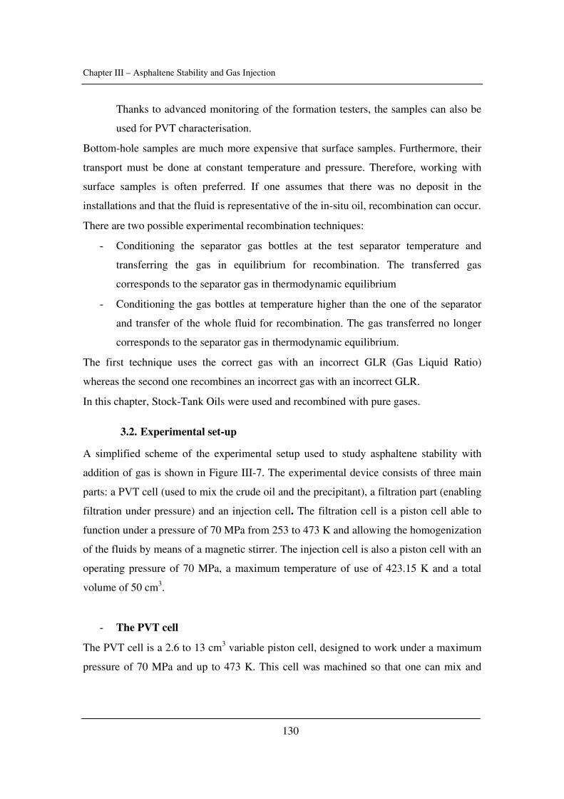
Chapter III – Asphaltene Stability and Gas Injection
130
Thanks to advanced monitoring of the formation testers, the samples can also be
used for PVT characterisation.
Bottom-hole samples are much more expensive that surface samples. Furthermore, their
transport must be done at constant temperature and pressure. Therefore, working with
surface samples is often preferred. If one assumes that there was no deposit in the
installations and that the fluid is representative of the in-situ oil, recombination can occur.
There are two possible experimental recombination techniques:
- Conditioning the separator gas bottles at the test separator temperature and
transferring the gas in equilibrium for recombination. The transferred gas
corresponds to the separator gas in thermodynamic equilibrium
- Conditioning the gas bottles at temperature higher than the one of the separator
and transfer of the whole fluid for recombination. The gas transferred no longer
corresponds to the separator gas in thermodynamic equilibrium.
The first technique uses the correct gas with an incorrect GLR (Gas Liquid Ratio)
whereas the second one recombines an incorrect gas with an incorrect GLR.
In this chapter, Stock-Tank Oils were used and recombined with pure gases.
3.2. Experimental set-up
A simplified scheme of the experimental setup used to study asphaltene stability with
addition of gas is shown in Figure III-7. The experimental device consists of three main
parts: a PVT cell (used to mix the crude oil and the precipitant), a filtration part (enabling
filtration under pressure) and an injection cell. The filtration cell is a piston cell able to
function under a pressure of 70 MPa from 253 to 473 K and allowing the homogenization
of the fluids by means of a magnetic stirrer. The injection cell is also a piston cell with an
operating pressure of 70 MPa, a maximum temperature of use of 423.15 K and a total
volume of 50 cm3.
- The PVT cell
The PVT cell is a 2.6 to 13 cm3 variable piston cell, designed to work under a maximum
pressure of 70 MPa and up to 473 K. This cell was machined so that one can mix and
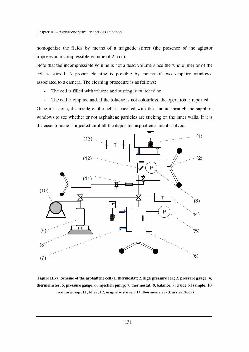
Chapter III – Asphaltene Stability and Gas Injection
131
homogenize the fluids by means of a magnetic stirrer (the presence of the agitator
imposes an incompressible volume of 2.6 cc).
Note that the incompressible volume is not a dead volume since the whole interior of the
cell is stirred. A proper cleaning is possible by means of two sapphire windows,
associated to a camera. The cleaning procedure is as follows:
- The cell is filled with toluene and stirring is switched on.
- The cell is emptied and, if the toluene is not colourless, the operation is repeated.
Once it is done, the inside of the cell is checked with the camera through the sapphire
windows to see whether or not asphaltene particles are sticking on the inner walls. If it is
the case, toluene is injected until all the deposited asphaltenes are dissolved.
Figure III-7: Scheme of the asphaltene cell (1, thermostat; 2, high pressure cell; 3, pressure gauge; 4,
thermometer; 5, pressure gauge; 6, injection pump; 7, thermostat; 8, balance; 9, crude oil sample; 10,
vacuum pump; 11, filter; 12, magnetic stirrer; 13, thermometer) (Carrier, 2005)
(6)
P
T
P
T
m
(1)
(3)
(4)
(11)
(2)
(5)
(10)
(9)
(8)
(7)
(13)
(12)
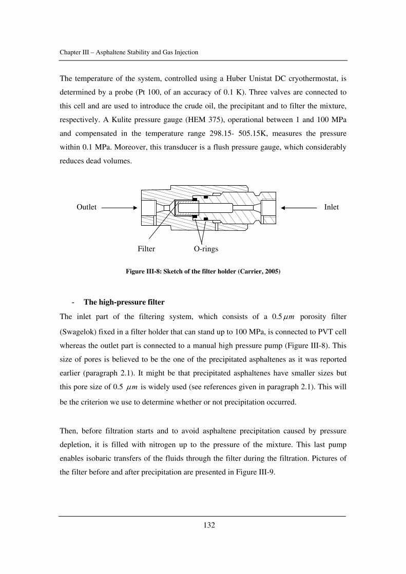
Chapter III – Asphaltene Stability and Gas Injection
132
The temperature of the system, controlled using a Huber Unistat DC cryothermostat, is
determined by a probe (Pt 100, of an accuracy of 0.1 K). Three valves are connected to
this cell and are used to introduce the crude oil, the precipitant and to filter the mixture,
respectively. A Kulite pressure gauge (HEM 375), operational between 1 and 100 MPa
and compensated in the temperature range 298.15- 505.15K, measures the pressure
within 0.1 MPa. Moreover, this transducer is a flush pressure gauge, which considerably
reduces dead volumes.
Figure III-8: Sketch of the filter holder (Carrier, 2005)
- The high-pressure filter
The inlet part of the filtering system, which consists of a 0.5 mμ porosity filter
(Swagelok) fixed in a filter holder that can stand up to 100 MPa, is connected to PVT cell
whereas the outlet part is connected to a manual high pressure pump (Figure III-8). This
size of pores is believed to be the one of the precipitated asphaltenes as it was reported
earlier (paragraph 2.1). It might be that precipitated asphaltenes have smaller sizes but
this pore size of 0.5 mμ is widely used (see references given in paragraph 2.1). This will
be the criterion we use to determine whether or not precipitation occurred.
Then, before filtration starts and to avoid asphaltene precipitation caused by pressure
depletion, it is filled with nitrogen up to the pressure of the mixture. This last pump
enables isobaric transfers of the fluids through the filter during the filtration. Pictures of
the filter before and after precipitation are presented in Figure III-9.
Filter O-rings
Inlet Outlet
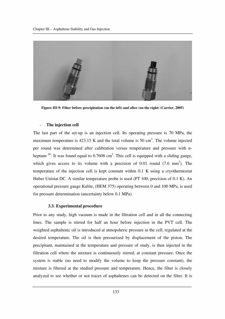
Chapter III – Asphaltene Stability and Gas Injection
133
Figure III-9: Filter before precipitation (on the left) and after (on the right) (Carrier, 2005)
- The injection cell
The last part of the set-up is an injection cell. Its operating pressure is 70 MPa, the
maximum temperature is 423.15 K and the total volume is 50 cm3. The volume injected
per round was determined after calibration versus temperature and pressure with n-
heptane 26. It was found equal to 0.7608 cm3. This cell is equipped with a sliding gauge,
which gives access to its volume with a precision of 0.01 round (7.6 mm3). The
temperature of the injection cell is kept constant within 0.1 K using a cryothermostat
Huber Unistat DC. A similar temperature probe is used (PT 100, precision of 0.1 K). An
operational pressure gauge Kulite, (HEM 375) operating between 0 and 100 MPa, is used
for pressure determination (uncertainty below 0.1 MPa).
3.3. Experimental procedure
Prior to any study, high vacuum is made in the filtration cell and in all the connecting
lines. The sample is stirred for half an hour before injection in the PVT cell. The
weighted asphaltenic oil is introduced at atmopsheric pressure in the cell, regulated at the
desired temperature. The oil is then pressurized by displacement of the piston. The
precipitant, maintained at the temperature and pressure of study, is then injected in the
filtration cell where the mixture is continuously stirred, at constant pressure. Once the
system is stable (no need to modify the volume to keep the pressure constant), the
mixture is filtered at the studied pressure and temperature. Hence, the filter is closely
analyzed to see whether or not traces of asphaltenes can be detected on the filter. It is
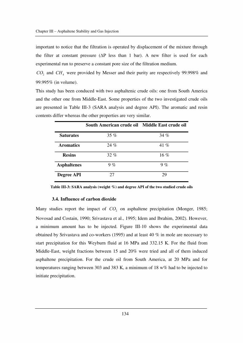
Chapter III – Asphaltene Stability and Gas Injection
134
important to notice that the filtration is operated by displacement of the mixture through
the filter at constant pressure (ΔP less than 1 bar). A new filter is used for each
experimental run to preserve a constant pore size of the filtration medium.
2CO and 4CH were provided by Messer and their purity are respectively 99.998% and
99.995% (in volume).
This study has been conduced with two asphaltenic crude oils: one from South America
and the other one from Middle-East. Some properties of the two investigated crude oils
are presented in Table III-3 (SARA analysis and degree API). The aromatic and resin
contents differ whereas the other properties are very similar.
South American crude oil Middle East crude oil
Saturates 35 % 34 %
Aromatics 24 % 41 %
Resins 32 % 16 %
Asphaltenes 9 % 9 %
Degree API 27 29
Table III-3: SARA analysis (weight %) and degree API of the two studied crude oils
3.4. Influence of carbon dioxide
Many studies report the impact of 2CO on asphaltene precipitation (Monger, 1985;
Novosad and Costain, 1990; Srivastava et al., 1995; Idem and Ibrahim, 2002). However,
a minimum amount has to be injected. Figure III-10 shows the experimental data
obtained by Srivastava and co-workers (1995) and at least 40 % in mole are necessary to
start precipitation for this Weyburn fluid at 16 MPa and 332.15 K. For the fluid from
Middle-East, weight fractions between 15 and 20% were tried and all of them induced
asphaltene precipitation. For the crude oil from South America, at 20 MPa and for
temperatures ranging between 303 and 383 K, a minimum of 18 w% had to be injected to
initiate precipitation.
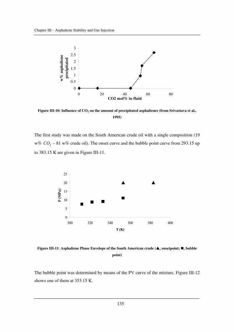
Chapter III – Asphaltene Stability and Gas Injection
135
0
0.5
1
1.5
2
2.5
3
0 20 40 60 80CO2 mol% in fluid
w%
asp
halt
ene
prec
ipit
ated
Figure III-10: Influence of CO2 on the amount of precipitated asphaltenes (from Srivastava et al.,
1995)
The first study was made on the South American crude oil with a single composition (19
w% 2CO – 81 w% crude oil). The onset curve and the bubble point curve from 293.15 up
to 383.15 K are given in Figure III-11.
0
5
10
15
20
25
300 320 340 360 380 400
T (K)
P (M
Pa)
Figure III-11: Asphaltene Phase Envelope of the South American crude ( , onsetpoint; , bubble
point)
The bubble point was determined by means of the PV curve of the mixture. Figure III-12
shows one of them at 353.15 K.
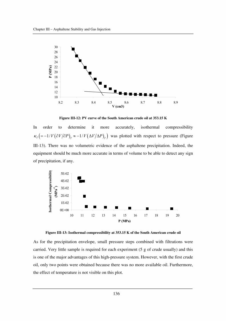
Chapter III – Asphaltene Stability and Gas Injection
136
1012141618202224262830
8.2 8.3 8.4 8.5 8.6 8.7 8.8 8.9V (cm3)
P (M
Pa)
Figure III-12: PV curve of the South American crude oil at 353.15 K
In order to determine it more accurately, isothermal compressibility
( ) ( )( )1/ 1/T T TV V P V V Pκ = − ∂ ∂ ≈ − Δ Δ was plotted with respect to pressure (Figure
III-13). There was no volumetric evidence of the asphaltene precipitation. Indeed, the
equipment should be much more accurate in terms of volume to be able to detect any sign
of precipitation, if any.
0E+00
1E-02
2E-02
3E-02
4E-02
5E-02
10 11 12 13 14 15 16 17 18 19 20P (MPa)
Isot
herm
al C
ompr
essi
bilit
y(M
Pa-1
)
Figure III-13: Isothermal compressibility at 353.15 K of the South American crude oil
As for the precipitation envelope, small pressure steps combined with filtrations were
carried. Very little sample is required for each experiment (5 g of crude usually) and this
is one of the major advantages of this high-pressure system. However, with the first crude
oil, only two points were obtained because there was no more available oil. Furthermore,
the effect of temperature is not visible on this plot.
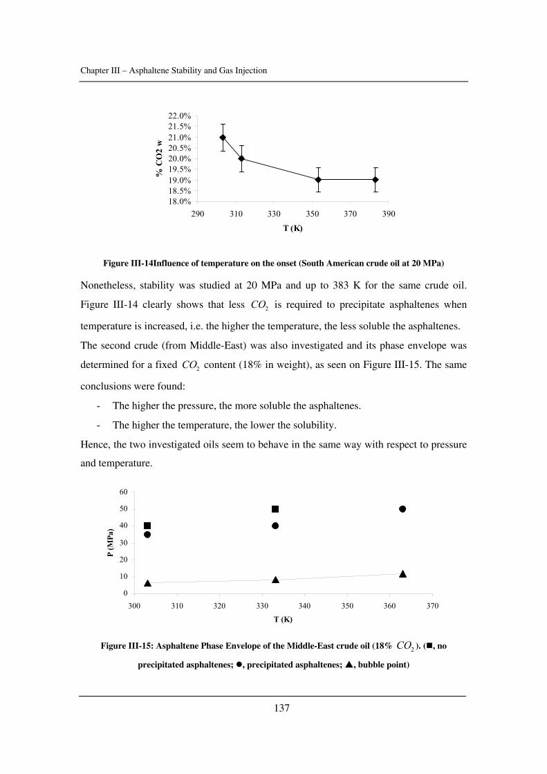
Chapter III – Asphaltene Stability and Gas Injection
137
18.0%18.5%19.0%19.5%20.0%20.5%21.0%21.5%22.0%
290 310 330 350 370 390
T (K)
% C
O2
w
Figure III-14Influence of temperature on the onset (South American crude oil at 20 MPa)
Nonetheless, stability was studied at 20 MPa and up to 383 K for the same crude oil.
Figure III-14 clearly shows that less 2CO is required to precipitate asphaltenes when
temperature is increased, i.e. the higher the temperature, the less soluble the asphaltenes.
The second crude (from Middle-East) was also investigated and its phase envelope was
determined for a fixed 2CO content (18% in weight), as seen on Figure III-15. The same
conclusions were found:
- The higher the pressure, the more soluble the asphaltenes.
- The higher the temperature, the lower the solubility.
Hence, the two investigated oils seem to behave in the same way with respect to pressure
and temperature.
0
10
20
30
40
50
60
300 310 320 330 340 350 360 370
T (K)
P (M
Pa)
Figure III-15: Asphaltene Phase Envelope of the Middle-East crude oil (18% 2CO ). ( , no
precipitated asphaltenes; , precipitated asphaltenes; , bubble point)
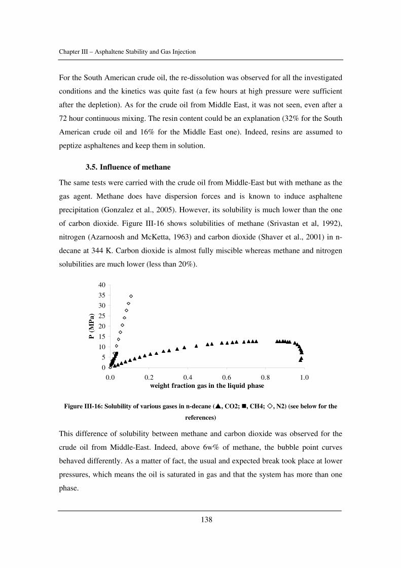
Chapter III – Asphaltene Stability and Gas Injection
138
For the South American crude oil, the re-dissolution was observed for all the investigated
conditions and the kinetics was quite fast (a few hours at high pressure were sufficient
after the depletion). As for the crude oil from Middle East, it was not seen, even after a
72 hour continuous mixing. The resin content could be an explanation (32% for the South
American crude oil and 16% for the Middle East one). Indeed, resins are assumed to
peptize asphaltenes and keep them in solution.
3.5. Influence of methane
The same tests were carried with the crude oil from Middle-East but with methane as the
gas agent. Methane does have dispersion forces and is known to induce asphaltene
precipitation (Gonzalez et al., 2005). However, its solubility is much lower than the one
of carbon dioxide. Figure III-16 shows solubilities of methane (Srivastan et al, 1992),
nitrogen (Azarnoosh and McKetta, 1963) and carbon dioxide (Shaver et al., 2001) in n-
decane at 344 K. Carbon dioxide is almost fully miscible whereas methane and nitrogen
solubilities are much lower (less than 20%).
0
5
10
15
20
25
30
35
40
0.0 0.2 0.4 0.6 0.8 1.0weight fraction gas in the liquid phase
P (
MP
a)
Figure III-16: Solubility of various gases in n-decane ( , CO2; , CH4; , N2) (see below for the
references)
This difference of solubility between methane and carbon dioxide was observed for the
crude oil from Middle-East. Indeed, above 6w% of methane, the bubble point curves
behaved differently. As a matter of fact, the usual and expected break took place at lower
pressures, which means the oil is saturated in gas and that the system has more than one
phase.

Chapter III – Asphaltene Stability and Gas Injection
139
The effect of temperature was studied for two methane concentrations (10 and 14 w%).
For those two concentrations, at 50 MPa, there were precipitated asphaltenes at 333.15 K
and none at 373.15 K. It means temperature has a stabilizing effect whereas it was the
contrary with 2CO for the same crude oil. Kokal and co-workers (Kokal et al., 1992)
mixed several light gases with two crude oils and measured the onset pressures between
298 and 373 K. With 2CO , temperature had both stabilizing and destabilizing effect
according to the oil under investigation. On the contrary, with light gases (ethane and
propane), there was a maximum in stability around 323 K for both oils. Methane had no
effect in terms of asphaltene precipitation. Hence, it is not unheard of for an oil to exhibit
different stability behaviours with different gases as it was found in this work.
The effect of concentration was also studied (at 333.15 K). The P-x diagram plotted in
Figure III-17 shows the experimental onset and bubble points. The full line represents
one possible phase envelope. It was chosen because no precipitate was detected with
2w% at any pressure whereas precipitated asphaltenes were detected at 4 and 6 w%.
0
5
10
15
20
25
30
0% 1% 2% 3% 4% 5% 6% 7% 8%
mass fraction CH4
P (M
Pa) Oil
Oil + Asphaltenes
Oil + Asphaltenes + Gas
Figure III-17: P-x diagram of the system crude oil Middle-East + Methane at 333.15 K ( , onset
point; , bubble point)
It is seen that the higher the methane content, the higher the bubble point pressure and the
onset pressure. The gap between the onset and the bubble point curves is quite small. The
re-dissolution curve (or lower onset curve) was not detected.
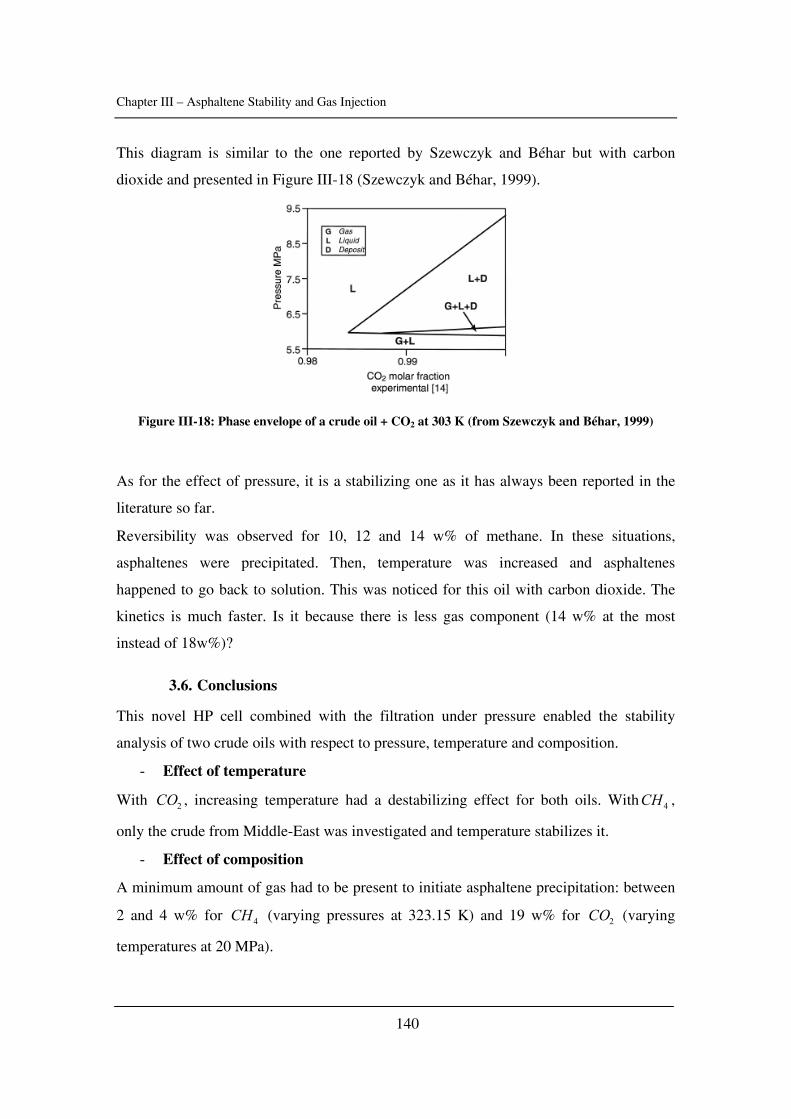
Chapter III – Asphaltene Stability and Gas Injection
140
This diagram is similar to the one reported by Szewczyk and Béhar but with carbon
dioxide and presented in Figure III-18 (Szewczyk and Béhar, 1999).
Figure III-18: Phase envelope of a crude oil + CO2 at 303 K (from Szewczyk and Béhar, 1999)
As for the effect of pressure, it is a stabilizing one as it has always been reported in the
literature so far.
Reversibility was observed for 10, 12 and 14 w% of methane. In these situations,
asphaltenes were precipitated. Then, temperature was increased and asphaltenes
happened to go back to solution. This was noticed for this oil with carbon dioxide. The
kinetics is much faster. Is it because there is less gas component (14 w% at the most
instead of 18w%)?
3.6. Conclusions
This novel HP cell combined with the filtration under pressure enabled the stability
analysis of two crude oils with respect to pressure, temperature and composition.
- Effect of temperature
With 2CO , increasing temperature had a destabilizing effect for both oils. With 4CH ,
only the crude from Middle-East was investigated and temperature stabilizes it.
- Effect of composition
A minimum amount of gas had to be present to initiate asphaltene precipitation: between
2 and 4 w% for 4CH (varying pressures at 323.15 K) and 19 w% for 2CO (varying
temperatures at 20 MPa).
Chapter III – Asphaltene Stability and Gas Injection
141
- Effect of pressure
The higher the pressure, the more soluble the asphaltenes for any gas injected.
This apparatus has a promising future since its working conditions are wide, the required
sample is small, the dead volume is inexistent, its cleaning is easy and the technique used
to determine asphaltene precipitation is not subject to doubts. Few apparatus dedicated to
the study of asphaltene solubility with pressure and temperature offer such advantages.
Furthermore, an optical device was developed lately on this cell. It brings interesting
input about the phase transitions (Castillo et al., 2006). The combination of both
techniques (filtration+ laser) will for sure improve the understanding of asphaltenic
fluids. Note that an automatic control and regulation of the pressure would improve this
experimental set-up. Appendix III-2 presents the article related to this work that will be
published in Energy & Fuels in 2006.
3.7. Unanswered issues and future work
Of course, several issues are still raising questions. A few of them are listed below:
- The pore size: a size of 0.5 mμ was chosen to detect the precipitated asphaltene
as it was done in several studies. Some analyses confirm such a size but a careful
study with a range of filters (from 0.1 to 1 mμ ) for instance would bring very
useful information. As a matter of fact, when does precipitation start? When the
size of the solids is 0.5 or 0.1 mμ ? The size-distribution studies carried by Montel
(2006) seem promising for that matter.
- Kinetics: is the thermodynamic equilibrium reached? In this work, filtration was
carried out once pressure was stable. It usually took between 5 and 24 hours. But,
kinetics can be very slow for asphaltenic fluids. It might be that asphaltenes were
not present in this work for some conditions but that they could have been a few
hours later. The use of the new laser system will permit to follow what “happens”
in the cell a bit more instead of working with a “black box” system.
Chapter III – Asphaltene Stability and Gas Injection
142
- Exact onset: in this work, filtrations were carried at different pressures to detect
the onset. The pressure difference between two tests was varying between 2.5 and
10 MPa. Smaller differences should be tested to obtain more accurate phase
envelopes.
- Reversibility: reversibility is highly related to kinetics. Precipitation was
reversible with methane and not carbon dioxide with the crude oil from Middle-
East. As it was said, the use of the laser with help detecting the reversibility and
obtaining the lower onset curves.
- Nitrogen: nitrogen is reported as a precipitant but no careful study presents its
effects on asphaltene stability. This experimental set-up should be used to perform
such an investigation.
Chapter III – Asphaltene Stability and Gas Injection
143
4. Conclusion
Gas injection was studied with a new high-pressure cell for two crude oils and two gases.
This technique detects precipitation and not flocculation (like many techniques do). The
determination of APE appeared to be time-consuming at the beginning but a better
knowledge of the experimental set-up enables fast measurements now (say 1-2 weeks to
obtain the PT-phase envelope of one defined mixture if nothing goes wrong).
The main issue is kinetics. But, this issue is valid for any measurements related to live
oils and asphaltene precipitation. How can one be 100% sure that the equilibrium is
reached? Hence, modelling of APE should be taken with care and perspective, especially
when the technique detects flocculation and not precipitation. Is it worth spending time
and money modelling “unreliable” data?
And last, but not least: even if a proper determination of an APE can be performed, how
representative is the studied sample?
Chapter III – Asphaltene Stability and Gas Injection
144
Literature
Akbarzadeh K., Alboudwarej H., Svrcek W., Yarranton H.W., A generalized regular solution model for asphaltene precipitation from n-alkane diluted heavy oils and bitumen, Fluid Phase Equilibr. (2005), 232, 159 - 170 Ali L.H., Al-Ghannam K.A., Investigations into asphaltenes in heavy crude oil. I. Effect of temperature on precipitation by alkane solvents, Fuel (1981), 60, 1043 – 1046 Andersen S.I., Effect of precipitation temperature on the composition of n-heptane asphaltenes, Fuel Sci.Techn. Int. (1994), 12, 51 – 74 Andersen S.I., Birdi K.S., Influence of temperature and solvent on the precipitation of asphaltenes, Fuel Sci.Techn. Int. (1990), 8, 593 – 615 Andersen S.I., Speight J.G., Thermodynamic models for asphaltene solubility and precipitation, J. Petrol. Sci. Eng. (1999), 22, 53 – 66 Andersen S.I., Flocculation onset titration of petroleum asphaltenes, Energ. Fuel. (1999), 13, 315 – 322 Aquino-Olivos M.A., Andersen S.I., Lira-Galeana C., Comparisons between asphaltenes from the dead and live-oil samples of the same crude oils, Pet. Sci. Technol. (2003), 21, 1017 – 1041 Aquino-Olivos M.A., Buenrostro-Gonzalez E., Andersen S.I., Lira-Galeana C., Investigations of inhibition of asphaltene precipitation at high pressure using bottomhole samples, Energ. Fuel.(2001), 15, 236-240 Azarnoosh A., McKetta J.J, Nitrogen-n-decane system in two-phase region, J. Chem. Eng. Data (1963), 8, 494-496 Briant J., Hotier G., Research on the state of asphaltenes in hydrocarbon mixtures – size of molecular clusters, Rev. I. Fr. Pet. (1983), 38, 83 – 100 Buckley J.S., Microscopic investigation of the onset of asphaltene precipitation (1996), Fuel Sci.Techn. Int. (1996), 14, 55 - 74 Buckley J.S., Predicting the onset of asphaltene precipitation from refractive index measurements, Energ. Fuel. (1999), 13, 328 – 332 Buckley J.S., Hirasaki G.J., Liu Y., Von Drasek S., Wang J.-X., Gill B.S., Asphaltene precipitation and solvent properties of crude oils, Pet. Sci. Technol. (1998), 16, 251 – 285
Chapter III – Asphaltene Stability and Gas Injection
145
Buenrostro-Gonzalez E., Lira-Galeana C., Gil-Villegas A., Wu J., Asphaltene precipitation in crude oils: theory and experiments, AIChE J. (2004), 50, 2552 – 2570 Burya Y.G., Yudin I.K., Dechabo V.A., Anisimon M.A., Colloidal properties of crude oils studied by dynamic light-scattering, Int. J. Thermophys. (2001), 22, 5, 1397 – 1410 Bushnell J.D., Ryan D.G., United States Patent No. 3976396, 1976 Carrier H., Laboratoire des Fluides Complexes, University of Pau, Personal communication (2005) Carrier H., Plantier F., Daridon J.-L., Lagourette B., Lu Z., Acoustic method for measuring asphaltene flocculation in crude oils, J. Petrol. Sci. Eng. (2000), 27, 111 - 117 Castillo J., Acevedo S., Canelon C.E., Carrier H., Daridon J.L., High pressure and high temperature investigations of asphaltene stability using an extrinsic refractometer, Energ. Fuel. (2006), accepted for publication Christensen A.A., Hadsbjerg C., Vestager-Tybjerg P.C., A study of the perturbed chain statistical associating fluid theory, Midterm Project: Technical University of Denmark, Department of Chemical Engineering, 2005 Clarke P.F., Pruden B.P, Asphaltene precipitation: detection using heat transfer analysis, and inhibition using chemical additives, Fuel, (1997), 76, 7, 607 – 614 Edmonds B., Moorwood R. A. S., Szczepanski R., Zhang X., Heyward M., Hurle R., Measurement and prediction of asphaltene precipitation from live oils, Proceedings of the third international symposium on colloid chemistry in oil production, asphaltenes and waxes deposition ( ISCOP'99 ), Mexico, November (1999) Ekulu G., Magri P., Rogalski M., Scanning aggregation phenomena in crude oils with density measurements, J. Dispers. Sci. Technol (2004), 25, 321 – 331 El-Mohamed S., Hardouin F., Gasparoux H., Floculation des produits lourds du pétrole, J. Chim. Phys. (1988), 85, 135 - 144 Escobedo J., Mansoori G.A.. Theory of viscosity as a criterion for detection of onset of asphaltene flocculation, Proceedings of the SPE International Petroleum Conference and Exhibition of Mexico, SPE 28729 (1994), 585 - 596 Fahim M.A., Dang T., Verdier S., Andersen S.I., Measurements of Precipitation of Asphaltenes from Live Oil Systems using a Filtration Technique, Presented at the 5th International Conference on Petroleum Phase Behaviour and Fouling, Banff, June 13 - 17, 2004.
Chapter III – Asphaltene Stability and Gas Injection
146
Fotland P., Anfindsen H., Fadnes F.H., Detection of asphaltene precipitation and amounts precipitated by measurement of electrical conductivity, Fluid Phase Equilibr. (1993), 82, 157 – 164 Fotland P., Precipitation of asphaltenes at high-pressures; Experimental technique and results, Fuel Sci.Techn. Int. (1996), 14, 313 – 325 Gonzalez D.L., Ting P.D., G.J. Hirasaki, Chapman W.G., Prediction of asphaltene instability Ander gas injection with the PC-SAFT equation of state, Energ. Fuel (2005), 19, 1230 - 1234 Hammami A., Phelps C.H., Monger-McClure T., Little T.M., Asphaltene precipitation from live oils: an experimental investigation of onset conditions and reversibility, Energ. Fuel. 2000, 14, 14 – 18 Hammami A., Chang-Yen D., Nighswander J.A., Stange E., An Experimental Study of the Effect of Paraffinic Solvents on the Onset and Bulk Precipitation of Asphaltenes, Fuel Sci.Techn. Int. (1995), 13, 1167-1184 Heithaus J.J., Measurement and significance of asphaltene peptization, J. Inst. Pet. (1962), 48, 45 – 53 Hirschberg A., deJong L.N.J., Schipper B.A., Meijer J.G., Influence of temperature and Pressure on asphaltene flocculation, paper SPE 11202, SPE J. (1984) 283 – 293 Hotier G., Robin M., Action de divers diluants sur les produits pétroliers lourds : mesure, interprétation et prévision de la floculation des asphaltenes, Rev. I. Fr. Petrol. (1983), 38, 1, 101 – 120 Hu Y.-F., Guo T.-M., Effect of temperature and molecular weight of n-alkane precipitants on asphaltene precipitation, Fluid Phase Equilibr. (2001), 192, 13 – 25 Knudsen L. B., Modelling of asphaltene precipitation; Master’s thesis: Technical University of Denmark, Department of Chemical Engineering, 2001. Idem R.O., Ibrahim H.H., Kinetics of CO2-induced asphaltene precipitation from various Saskatchewan crude oils during CO2 miscible flooding, J. Pet. Sci. Eng. (2002), 35, 233 – 246 Jamaluddin A.K.M., Creek J., Kabir C.S., McFadden J.D., D'Cruz D., Manakalathil J., Joshi N., Ross B., J. Can. Pet. Technol. (2002), 41, 44 - 52 Jamaluddin A.K.M., Joshi N., Iwere F., Gurpinar O., An Investigation of Asphaltene Instability under Nitrogen Injection, Proceedings of the SPE International Petroleum Conference and Exhibition of Mexico (2002), 427 – 436
Chapter III – Asphaltene Stability and Gas Injection
147
Joshi N.B., Mullins O.C., Jamaluddin A., Creek J., McFadden J., Asphaltene precipitation from live crude oil, Energ. Fuel. (2001), 15, 979 – 986 Kokal S.L., Najman J., Sayegh S.G., George A.E., Measurement and correlation of asphaltene precipitation from heavy oils by gas injection, J. Can. Petrol. Technol. (1992), 31, 24-30 Le Châtelier, H. L. Ann. Mines (1888), 13, 157 Laux H., Rahimian I., Browarzik D., Floculation of asphaltenes at high pressure. I – Experimental determination of the onset of flocculation, Pet. Sci. Technol. (2001), 19, 1155 – 166 Leontaritis K.J., The asphaltene and wax deposition envelopes, Fuel Sci.Techn. Int. (1996), 14, 13 – 39 Leontaritis K.J., Amaefule J.O., Charles R.E., Systematic approach for the prevention and treatment of formation damage caused by asphaltene deposition, SPE Prod. Facil. (1994), 9, 157-164 Lhioreau C., Briant J., Tindy R., Influence de la pression sur la floculation des asphaltenes, Rev. I. Fr. Petrol. (1967), 22, 5, 797 – 806 Lu Z., Daridon J.L., Lagourette B., Ye S., Phase comparison technique for measuring liquid-liquid phase equilibrium, Rev. Sci. Instrum. (1999), 70, 2065-2068 Monger T.G., The impact of oil aromaticity on carbon dioxide flooding, SPE J. (1985), 25, 371 – 378 Montel F., Petroleum Thermodynamics, Notes, Total, 2004 Montel V., Laboratoire des Fluides Complexes, University of Pau, Personal communication (2006) Negahban S., Bahamaish J.N.M., Joshi N., Nighswander J., Jamaluddin A.K.M., An experimental study at an Abu Dhabi reservoir of asphaltene precipitation caused by gas injection, SPE Prod. .Facil. (2005), 20, 115-125 Novosad Z., Costain T.G., Experimental and modelling studies of asphaltene equilibria for a reservoir under CO2 injection, SPE 20530 (1990), 599 - 607 Peramanu S., Clarke P.F., Pruden B.B., Flow loop apparatus to study the effect of solvent, temperature and additives on asphaltene precipitation, J. Petrol. Sci. Eng. (1999), 23, 133–143
Chapter III – Asphaltene Stability and Gas Injection
148
Shaver R.D., Robinson R.L., Gasem K.A.M., An automated apparatus for equilibrium phase compositions, densities, and interfacial tensions: data for carbon dioxide + decane, Fluid Phase Equilibr. (2001), 179, 43–66 Shaw J.M., Béhar E., SLLV phase behavior and phase diagram transitions in asymmetric hydrocarbon fluids, Fluid Phase Equilibr. (2003), 209, 185 – 206 Srivastan S., Darwish N.A., Gasem K.A.M., Robinson R.L. Jr., Solubility of methane in hexane, decane, and dodecane at temperatures from 311 to 423 K and pressures to 10.4 MPa, J. Chem. Eng. Data (1992), 37, 516 - 520 Srivastava R.K., Huang S.S., Dyer S.B., Mourits, F.M., Quantification of asphaltene flocculation during miscible CO2 flooding in the Weyburn reservoir, J. Can. Pet. Tech. (1995), 34, 31 – 42 Stachowiak C., Grolier J.-P.E., Randzio S.L., Transitiometric investigation of asphaltenic fluids under in-well pressure and temperature conditions, Energ. Fuel. (2001), 15, 1033 – 1037 Szewczyk V., Béhar E., Compositional model for predicting asphaltenes flocculation, Fluid Phase Equilibr. (1999), 158, 459 – 469
Chapter IV – Asphaltene Precipitation and Calorimetry
149
Chapter IV
Asphaltene Precipitation and Calorimetry
Chapter IV – Asphaltene Precipitation and Calorimetry
150
Table of Contents
1. Review .................................................................................................................... 152
1.1. Brief note about exo- and endothermy........................................................... 152
1.2. Mixtures of Asphaltenes and crude oils with aromatics and n-alkanes .......... 153
1.2.1. Dilution of asphaltene solutions.............................................................. 154
1.2.2. Dilution of crude oils .............................................................................. 156
1.3. Precipitation .................................................................................................... 157
1.4. Other calorimetric studies ............................................................................... 158
1.5. Conclusion ...................................................................................................... 159
2. Asphaltene precipitation and Isothermal Titration Calorimetry..................... 160
2.1. Description of the ITC equipment .................................................................. 160
2.2. ITC and Phase transitions ............................................................................... 161
2.3. ITC and Asphaltene Precipitation................................................................... 165
2.3.1. Asphaltene solutions ............................................................................... 165
2.3.2. Crude oil.................................................................................................. 168
3. Asphaltene precipitation and high pressure calorimetry.................................. 170
3.1. Experimental set-up ........................................................................................ 171
3.2. The system under investigation ...................................................................... 172
3.3. Variations of temperature ............................................................................... 173
3.4. Pressure depletion ........................................................................................... 175
3.5. Discussion and Conclusion............................................................................. 176
4. Conclusion about calorimetry.............................................................................. 178
Literature....................................................................................................................... 179
Chapter IV – Asphaltene Precipitation and Calorimetry
151
What is asphaltene precipitation about in terms of calorimetry? Can calorimetry help
predicting the influence of temperature on stability, as the Le Châtelier’s principle predict
it? What has been done in that area so far? Can calorimetry help understanding
precipitation and other aggregation phenomena?
First, a brief literature review will explain the different works done with dilution and
precipitation of asphaltenic systems. Then, the attempt to follow asphaltene precipitation
induced by n-heptane by Isothermal Titration Calorimetry will be presented. Finally,
some experiments carried out will live oils in a HP calorimeter will be described and
explained.
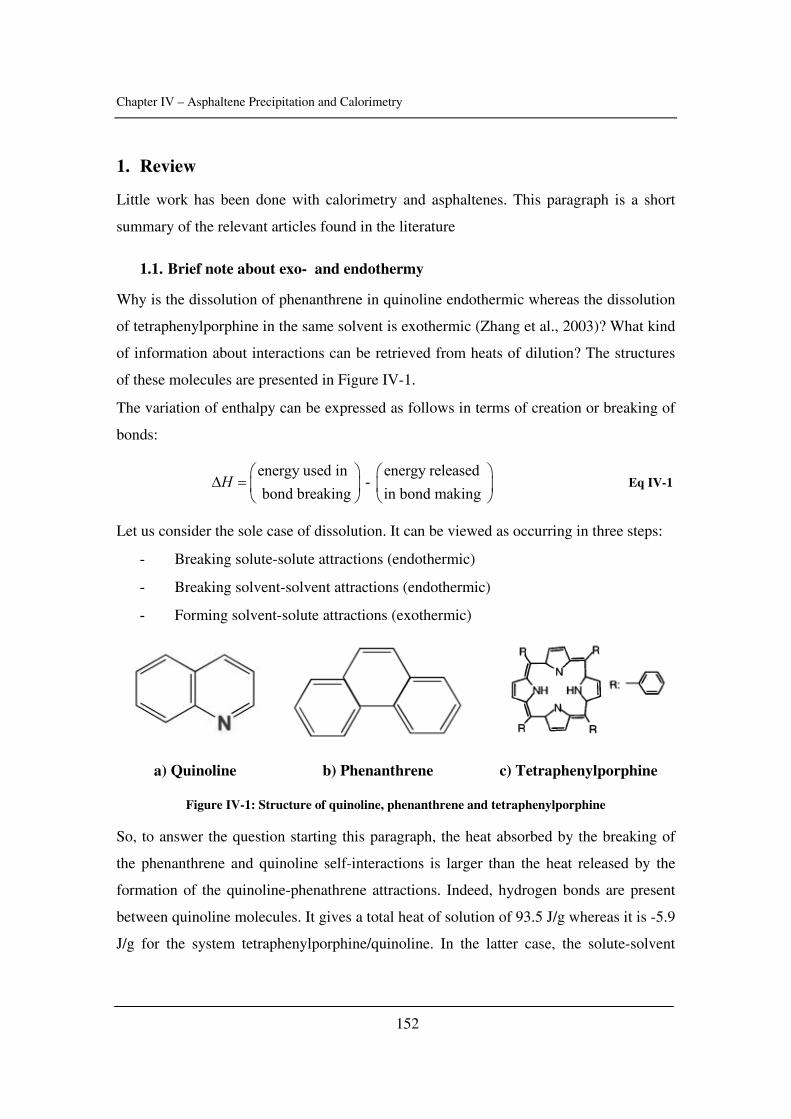
Chapter IV – Asphaltene Precipitation and Calorimetry
152
1. Review
Little work has been done with calorimetry and asphaltenes. This paragraph is a short
summary of the relevant articles found in the literature
1.1. Brief note about exo- and endothermy
Why is the dissolution of phenanthrene in quinoline endothermic whereas the dissolution
of tetraphenylporphine in the same solvent is exothermic (Zhang et al., 2003)? What kind
of information about interactions can be retrieved from heats of dilution? The structures
of these molecules are presented in Figure IV-1.
The variation of enthalpy can be expressed as follows in terms of creation or breaking of
bonds:
energy used in energy released -
bond breaking in bond makingH
⎛ ⎞ ⎛ ⎞Δ = ⎜ ⎟ ⎜ ⎟
⎝ ⎠ ⎝ ⎠ Eq IV-1
Let us consider the sole case of dissolution. It can be viewed as occurring in three steps:
- Breaking solute-solute attractions (endothermic)
- Breaking solvent-solvent attractions (endothermic)
- Forming solvent-solute attractions (exothermic)
a) Quinoline b) Phenanthrene c) Tetraphenylporphine
Figure IV-1: Structure of quinoline, phenanthrene and tetraphenylporphine
So, to answer the question starting this paragraph, the heat absorbed by the breaking of
the phenanthrene and quinoline self-interactions is larger than the heat released by the
formation of the quinoline-phenathrene attractions. Indeed, hydrogen bonds are present
between quinoline molecules. It gives a total heat of solution of 93.5 J/g whereas it is -5.9
J/g for the system tetraphenylporphine/quinoline. In the latter case, the solute-solvent
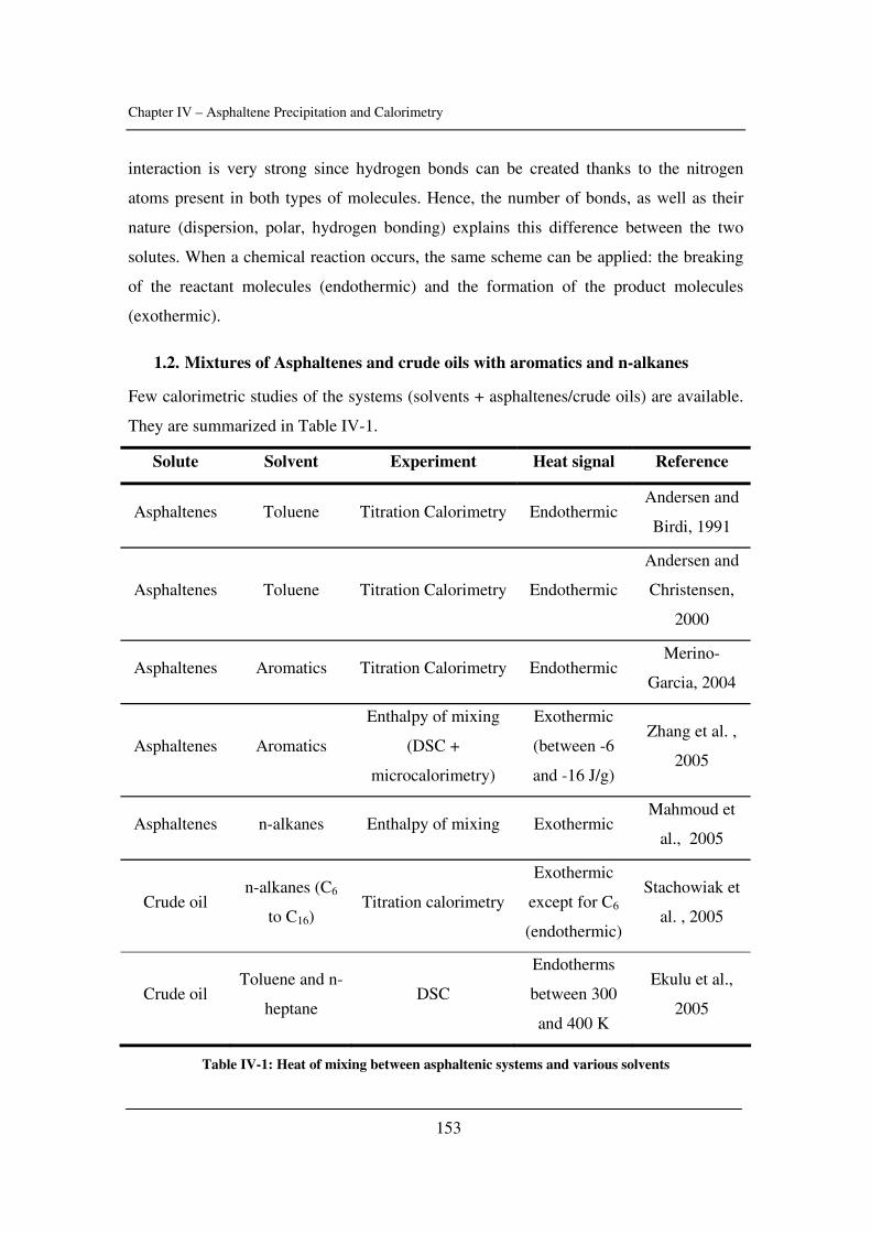
Chapter IV – Asphaltene Precipitation and Calorimetry
153
interaction is very strong since hydrogen bonds can be created thanks to the nitrogen
atoms present in both types of molecules. Hence, the number of bonds, as well as their
nature (dispersion, polar, hydrogen bonding) explains this difference between the two
solutes. When a chemical reaction occurs, the same scheme can be applied: the breaking
of the reactant molecules (endothermic) and the formation of the product molecules
(exothermic).
1.2. Mixtures of Asphaltenes and crude oils with aromatics and n-alkanes
Few calorimetric studies of the systems (solvents + asphaltenes/crude oils) are available.
They are summarized in Table IV-1.
Solute Solvent Experiment Heat signal Reference
Asphaltenes Toluene Titration Calorimetry Endothermic Andersen and
Birdi, 1991
Asphaltenes Toluene Titration Calorimetry Endothermic
Andersen and
Christensen,
2000
Asphaltenes Aromatics Titration Calorimetry Endothermic Merino-
Garcia, 2004
Asphaltenes Aromatics
Enthalpy of mixing
(DSC +
microcalorimetry)
Exothermic
(between -6
and -16 J/g)
Zhang et al. ,
2005
Asphaltenes n-alkanes Enthalpy of mixing Exothermic Mahmoud et
al., 2005
Crude oil n-alkanes (C6
to C16) Titration calorimetry
Exothermic
except for C6
(endothermic)
Stachowiak et
al. , 2005
Crude oil Toluene and n-
heptane DSC
Endotherms
between 300
and 400 K
Ekulu et al.,
2005
Table IV-1: Heat of mixing between asphaltenic systems and various solvents
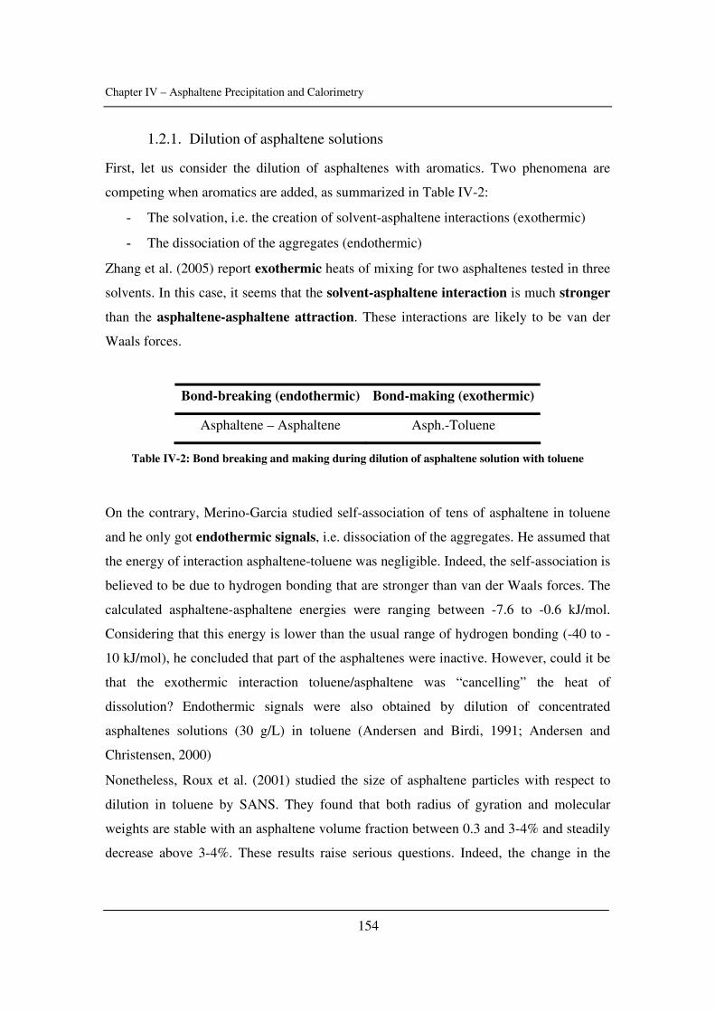
Chapter IV – Asphaltene Precipitation and Calorimetry
154
1.2.1. Dilution of asphaltene solutions
First, let us consider the dilution of asphaltenes with aromatics. Two phenomena are
competing when aromatics are added, as summarized in Table IV-2:
- The solvation, i.e. the creation of solvent-asphaltene interactions (exothermic)
- The dissociation of the aggregates (endothermic)
Zhang et al. (2005) report exothermic heats of mixing for two asphaltenes tested in three
solvents. In this case, it seems that the solvent-asphaltene interaction is much stronger
than the asphaltene-asphaltene attraction. These interactions are likely to be van der
Waals forces.
Bond-breaking (endothermic) Bond-making (exothermic)
Asphaltene – Asphaltene Asph.-Toluene
Table IV-2: Bond breaking and making during dilution of asphaltene solution with toluene
On the contrary, Merino-Garcia studied self-association of tens of asphaltene in toluene
and he only got endothermic signals, i.e. dissociation of the aggregates. He assumed that
the energy of interaction asphaltene-toluene was negligible. Indeed, the self-association is
believed to be due to hydrogen bonding that are stronger than van der Waals forces. The
calculated asphaltene-asphaltene energies were ranging between -7.6 to -0.6 kJ/mol.
Considering that this energy is lower than the usual range of hydrogen bonding (-40 to -
10 kJ/mol), he concluded that part of the asphaltenes were inactive. However, could it be
that the exothermic interaction toluene/asphaltene was “cancelling” the heat of
dissolution? Endothermic signals were also obtained by dilution of concentrated
asphaltenes solutions (30 g/L) in toluene (Andersen and Birdi, 1991; Andersen and
Christensen, 2000)
Nonetheless, Roux et al. (2001) studied the size of asphaltene particles with respect to
dilution in toluene by SANS. They found that both radius of gyration and molecular
weights are stable with an asphaltene volume fraction between 0.3 and 3-4% and steadily
decrease above 3-4%. These results raise serious questions. Indeed, the change in the
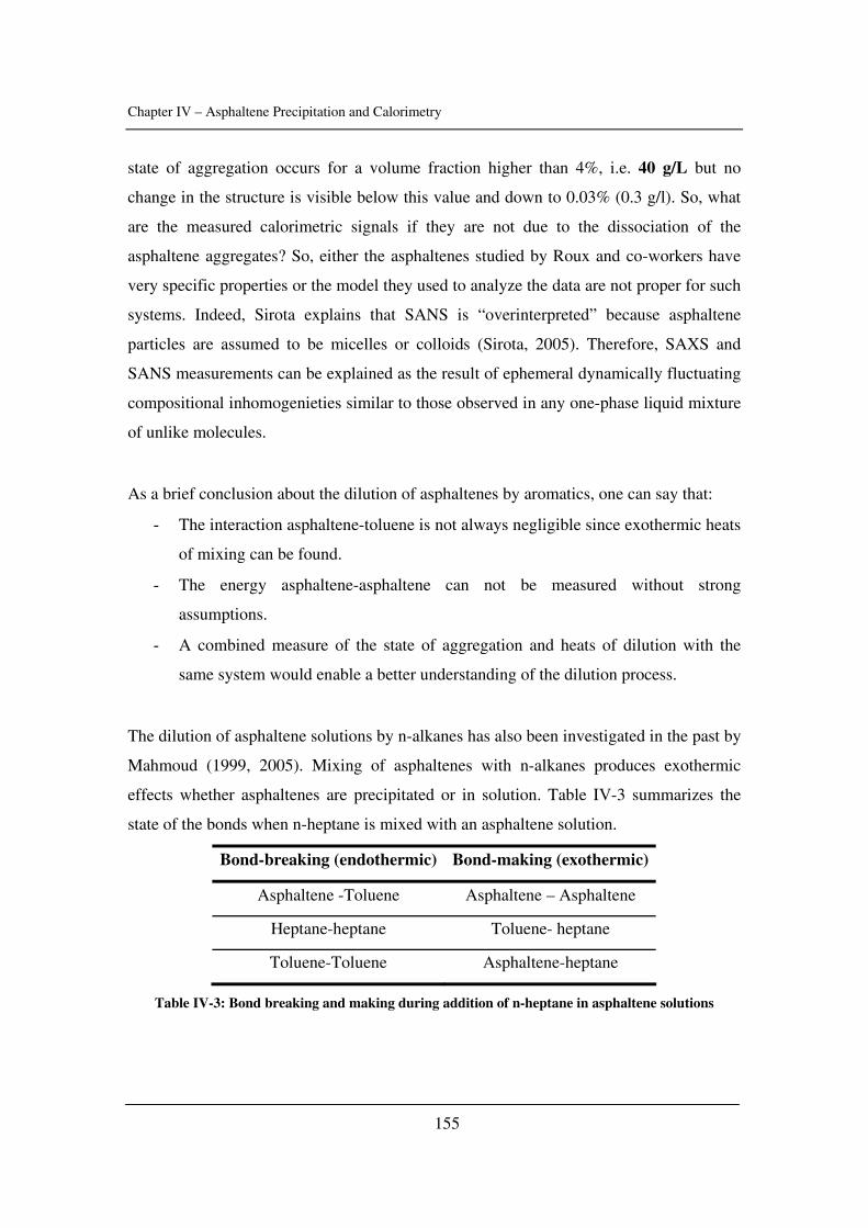
Chapter IV – Asphaltene Precipitation and Calorimetry
155
state of aggregation occurs for a volume fraction higher than 4%, i.e. 40 g/L but no
change in the structure is visible below this value and down to 0.03% (0.3 g/l). So, what
are the measured calorimetric signals if they are not due to the dissociation of the
asphaltene aggregates? So, either the asphaltenes studied by Roux and co-workers have
very specific properties or the model they used to analyze the data are not proper for such
systems. Indeed, Sirota explains that SANS is “overinterpreted” because asphaltene
particles are assumed to be micelles or colloids (Sirota, 2005). Therefore, SAXS and
SANS measurements can be explained as the result of ephemeral dynamically fluctuating
compositional inhomogenieties similar to those observed in any one-phase liquid mixture
of unlike molecules.
As a brief conclusion about the dilution of asphaltenes by aromatics, one can say that:
- The interaction asphaltene-toluene is not always negligible since exothermic heats
of mixing can be found.
- The energy asphaltene-asphaltene can not be measured without strong
assumptions.
- A combined measure of the state of aggregation and heats of dilution with the
same system would enable a better understanding of the dilution process.
The dilution of asphaltene solutions by n-alkanes has also been investigated in the past by
Mahmoud (1999, 2005). Mixing of asphaltenes with n-alkanes produces exothermic
effects whether asphaltenes are precipitated or in solution. Table IV-3 summarizes the
state of the bonds when n-heptane is mixed with an asphaltene solution.
Bond-breaking (endothermic) Bond-making (exothermic)
Asphaltene -Toluene Asphaltene – Asphaltene
Heptane-heptane Toluene- heptane
Toluene-Toluene Asphaltene-heptane
Table IV-3: Bond breaking and making during addition of n-heptane in asphaltene solutions
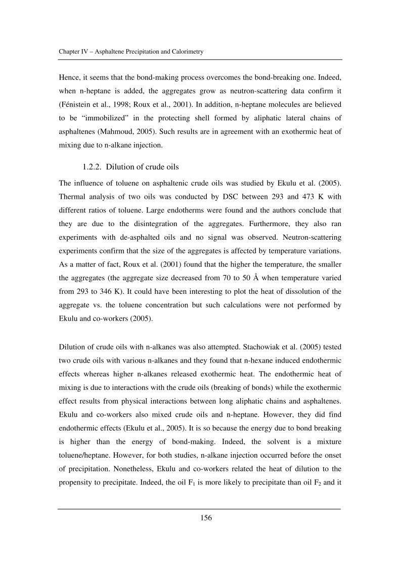
Chapter IV – Asphaltene Precipitation and Calorimetry
156
Hence, it seems that the bond-making process overcomes the bond-breaking one. Indeed,
when n-heptane is added, the aggregates grow as neutron-scattering data confirm it
(Fénistein et al., 1998; Roux et al., 2001). In addition, n-heptane molecules are believed
to be “immobilized” in the protecting shell formed by aliphatic lateral chains of
asphaltenes (Mahmoud, 2005). Such results are in agreement with an exothermic heat of
mixing due to n-alkane injection.
1.2.2. Dilution of crude oils
The influence of toluene on asphaltenic crude oils was studied by Ekulu et al. (2005).
Thermal analysis of two oils was conducted by DSC between 293 and 473 K with
different ratios of toluene. Large endotherms were found and the authors conclude that
they are due to the disintegration of the aggregates. Furthermore, they also ran
experiments with de-asphalted oils and no signal was observed. Neutron-scattering
experiments confirm that the size of the aggregates is affected by temperature variations.
As a matter of fact, Roux et al. (2001) found that the higher the temperature, the smaller
the aggregates (the aggregate size decreased from 70 to 50 Å when temperature varied
from 293 to 346 K). It could have been interesting to plot the heat of dissolution of the
aggregate vs. the toluene concentration but such calculations were not performed by
Ekulu and co-workers (2005).
Dilution of crude oils with n-alkanes was also attempted. Stachowiak et al. (2005) tested
two crude oils with various n-alkanes and they found that n-hexane induced endothermic
effects whereas higher n-alkanes released exothermic heat. The endothermic heat of
mixing is due to interactions with the crude oils (breaking of bonds) while the exothermic
effect results from physical interactions between long aliphatic chains and asphaltenes.
Ekulu and co-workers also mixed crude oils and n-heptane. However, they did find
endothermic effects (Ekulu et al., 2005). It is so because the energy due to bond breaking
is higher than the energy of bond-making. Indeed, the solvent is a mixture
toluene/heptane. However, for both studies, n-alkane injection occurred before the onset
of precipitation. Nonetheless, Ekulu and co-workers related the heat of dilution to the
propensity to precipitate. Indeed, the oil F1 is more likely to precipitate than oil F2 and it
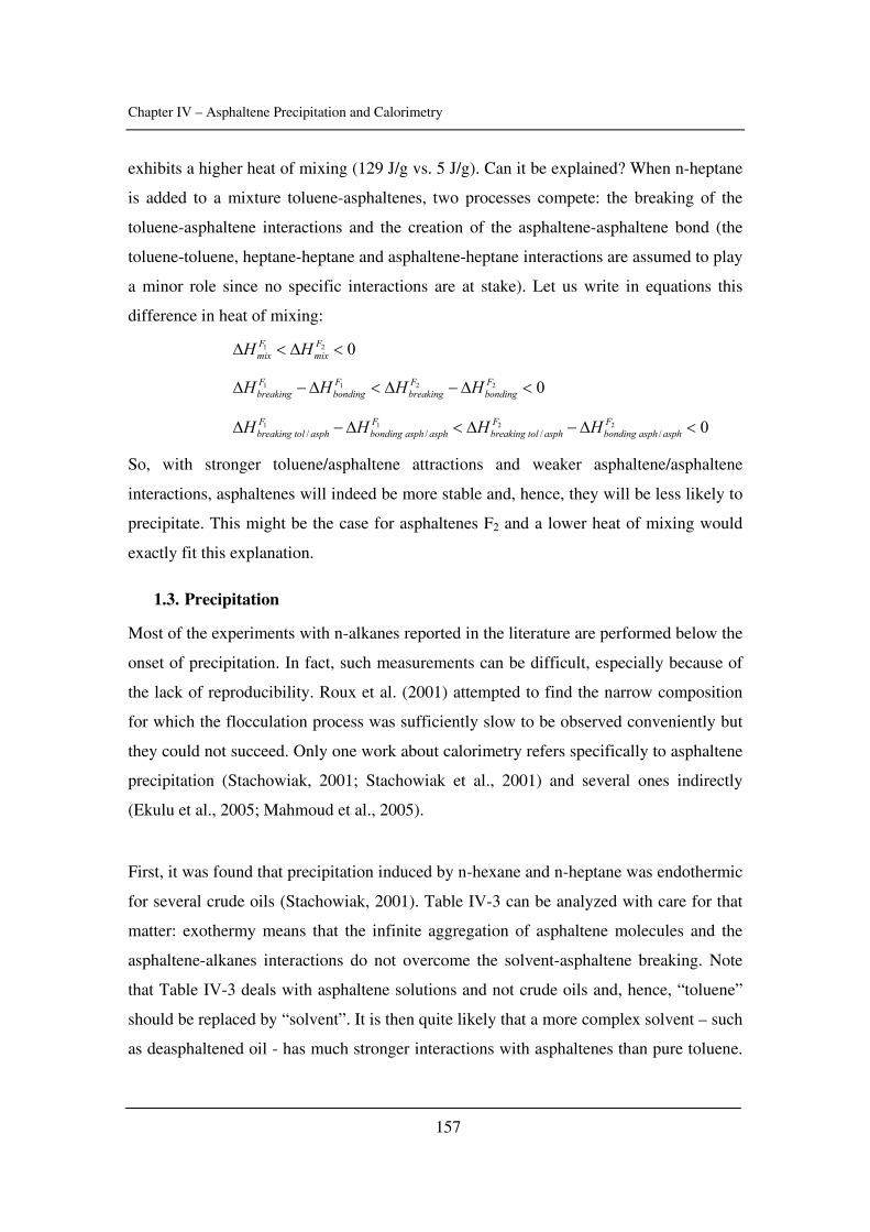
Chapter IV – Asphaltene Precipitation and Calorimetry
157
exhibits a higher heat of mixing (129 J/g vs. 5 J/g). Can it be explained? When n-heptane
is added to a mixture toluene-asphaltenes, two processes compete: the breaking of the
toluene-asphaltene interactions and the creation of the asphaltene-asphaltene bond (the
toluene-toluene, heptane-heptane and asphaltene-heptane interactions are assumed to play
a minor role since no specific interactions are at stake). Let us write in equations this
difference in heat of mixing:
1 2 0F Fmix mixH HΔ < Δ <
1 1 2 2 0F F F Fbreaking bonding breaking bondingH H H HΔ −Δ < Δ −Δ <
1 1 2 2/ / / / 0F F F F
breaking tol asph bonding asph asph breaking tol asph bonding asph asphH H H HΔ −Δ < Δ −Δ <
So, with stronger toluene/asphaltene attractions and weaker asphaltene/asphaltene
interactions, asphaltenes will indeed be more stable and, hence, they will be less likely to
precipitate. This might be the case for asphaltenes F2 and a lower heat of mixing would
exactly fit this explanation.
1.3. Precipitation
Most of the experiments with n-alkanes reported in the literature are performed below the
onset of precipitation. In fact, such measurements can be difficult, especially because of
the lack of reproducibility. Roux et al. (2001) attempted to find the narrow composition
for which the flocculation process was sufficiently slow to be observed conveniently but
they could not succeed. Only one work about calorimetry refers specifically to asphaltene
precipitation (Stachowiak, 2001; Stachowiak et al., 2001) and several ones indirectly
(Ekulu et al., 2005; Mahmoud et al., 2005).
First, it was found that precipitation induced by n-hexane and n-heptane was endothermic
for several crude oils (Stachowiak, 2001). Table IV-3 can be analyzed with care for that
matter: exothermy means that the infinite aggregation of asphaltene molecules and the
asphaltene-alkanes interactions do not overcome the solvent-asphaltene breaking. Note
that Table IV-3 deals with asphaltene solutions and not crude oils and, hence, “toluene”
should be replaced by “solvent”. It is then quite likely that a more complex solvent – such
as deasphaltened oil - has much stronger interactions with asphaltenes than pure toluene.
Chapter IV – Asphaltene Precipitation and Calorimetry
158
For instance, resins have strong interactions with asphaltenes since 1 cm3 of resins had
the same dispersing power as 105 cm3 of benzene (Hotier and Robin, 1983).
When precipitation is caused by pressure depletion (Stachowiak et al., 2001), exothermic
signals are found. Table IV-4 lists the different bonds broken and created.
Bond-breaking (endothermic) Bond-making (exothermic)
Asphaltene -solvent Asphaltene – Asphaltene
Solvent-solvent
Table IV-4: State of the interactions during pressure depletion of crude oils
Since more bonds are created than broken, it does seem logical that precipitation caused
by pressure depletion is exothermic. As a matter of fact, precipitation is often described
as an infinite aggregation (Fénistein, 1998).
In terms of Le Châtelier’s principle (Chapter 3, paragraph 1.4), what can be learnt from
such experiments? As it was concluded in Chapter 3, an endothermic precipitation means
that an increase temperature would destabilize solubilised asphaltenes. Unfortunately, in
the mentioned works, the impact of temperature on stability was not studied.
Nonetheless, it would mean that the n-heptane induced asphaltenes (Stachowiak, 2001)
would precipitate with temperature. On the contrary, the live oil (Stachowiak et al., 2001)
would be more stable with higher temperatures.
1.4. Other calorimetric studies
Andersen et al. (2001) studied the interaction between water and asphaltenes in solutions.
It appeared that the CMC could be assigned to the water content. Indeed, after drying the
toluene used for titration calorimetry, the break that was assumed to be due to a CMC
disappeared.
Merino-Garcia (2004) studied the interaction asphaltene-resin. He found that stable oils
had more interaction with a model resin (nonylphenol) than unstable crude oils. The
Chapter IV – Asphaltene Precipitation and Calorimetry
159
number of sites was estimated as well (no more heat of interaction). Furthermore, no
correlation between heat of interaction asphaltene-resins and stability was found.
Glass transitions have also been measured for asphaltenes by DSC. Zhang et al. (2004)
list the work done previously on that matter. The glass transition range is reported
between 100 and 180°C.
1.5. Conclusion
No solvent is inert and, hence, determination of interactions energy requires assumptions.
Obviously, calorimetric data show that precipitation caused by pressure or temperature
variations is different from the one caused by n-alkanes. Indeed, the same interactions are
not involved. As a matter of fact, as it was said in chapter 1, paragraph 1.1, the
differences between “pressure-depleted asphaltenes” and n-heptane asphaltenes are
massive (distribution, composition, etc…).
Furthermore, calorimetry has not been used very much for asphaltenic systems whereas it
has great potentials to understand aggregation and precipitation. However, the time when
calorimetry will enable predictions about asphaltene precipitations is out of reach with
today’s work. Do heats of mixing contain information about stability? The following
paragraphs will be focused on this question.
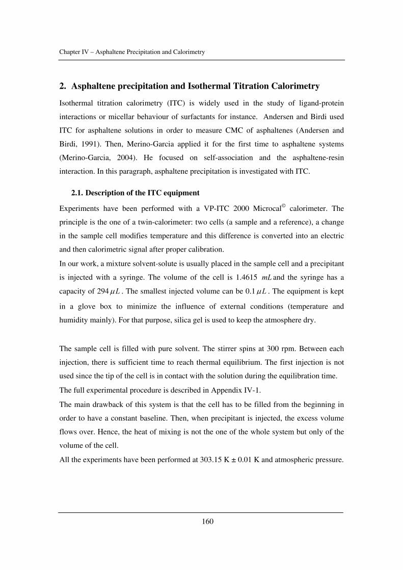
Chapter IV – Asphaltene Precipitation and Calorimetry
160
2. Asphaltene precipitation and Isothermal Titration Calorimetry
Isothermal titration calorimetry (ITC) is widely used in the study of ligand-protein
interactions or micellar behaviour of surfactants for instance. Andersen and Birdi used
ITC for asphaltene solutions in order to measure CMC of asphaltenes (Andersen and
Birdi, 1991). Then, Merino-Garcia applied it for the first time to asphaltene systems
(Merino-Garcia, 2004). He focused on self-association and the asphaltene-resin
interaction. In this paragraph, asphaltene precipitation is investigated with ITC.
2.1. Description of the ITC equipment
Experiments have been performed with a VP-ITC 2000 Microcal© calorimeter. The
principle is the one of a twin-calorimeter: two cells (a sample and a reference), a change
in the sample cell modifies temperature and this difference is converted into an electric
and then calorimetric signal after proper calibration.
In our work, a mixture solvent-solute is usually placed in the sample cell and a precipitant
is injected with a syringe. The volume of the cell is 1.4615 mL and the syringe has a
capacity of 294 Lμ . The smallest injected volume can be 0.1 Lμ . The equipment is kept
in a glove box to minimize the influence of external conditions (temperature and
humidity mainly). For that purpose, silica gel is used to keep the atmosphere dry.
The sample cell is filled with pure solvent. The stirrer spins at 300 rpm. Between each
injection, there is sufficient time to reach thermal equilibrium. The first injection is not
used since the tip of the cell is in contact with the solution during the equilibration time.
The full experimental procedure is described in Appendix IV-1.
The main drawback of this system is that the cell has to be filled from the beginning in
order to have a constant baseline. Then, when precipitant is injected, the excess volume
flows over. Hence, the heat of mixing is not the one of the whole system but only of the
volume of the cell.
All the experiments have been performed at 303.15 K ± 0.01 K and atmospheric pressure.
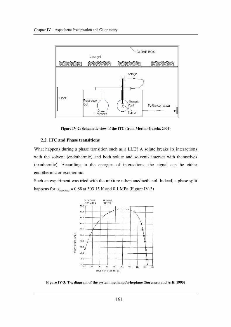
Chapter IV – Asphaltene Precipitation and Calorimetry
161
Figure IV-2: Schematic view of the ITC (from Merino-Garcia, 2004)
2.2. ITC and Phase transitions
What happens during a phase transition such as a LLE? A solute breaks its interactions
with the solvent (endothermic) and both solute and solvents interact with themselves
(exothermic). According to the energies of interactions, the signal can be either
endothermic or exothermic.
Such an experiment was tried with the mixture n-heptane/methanol. Indeed, a phase split
happens for 0.88methanolx = at 303.15 K and 0.1 MPa (Figure IV-3)
Figure IV-3: T-x diagram of the system methanol/n-heptane (Sørensen and Arlt, 1995)
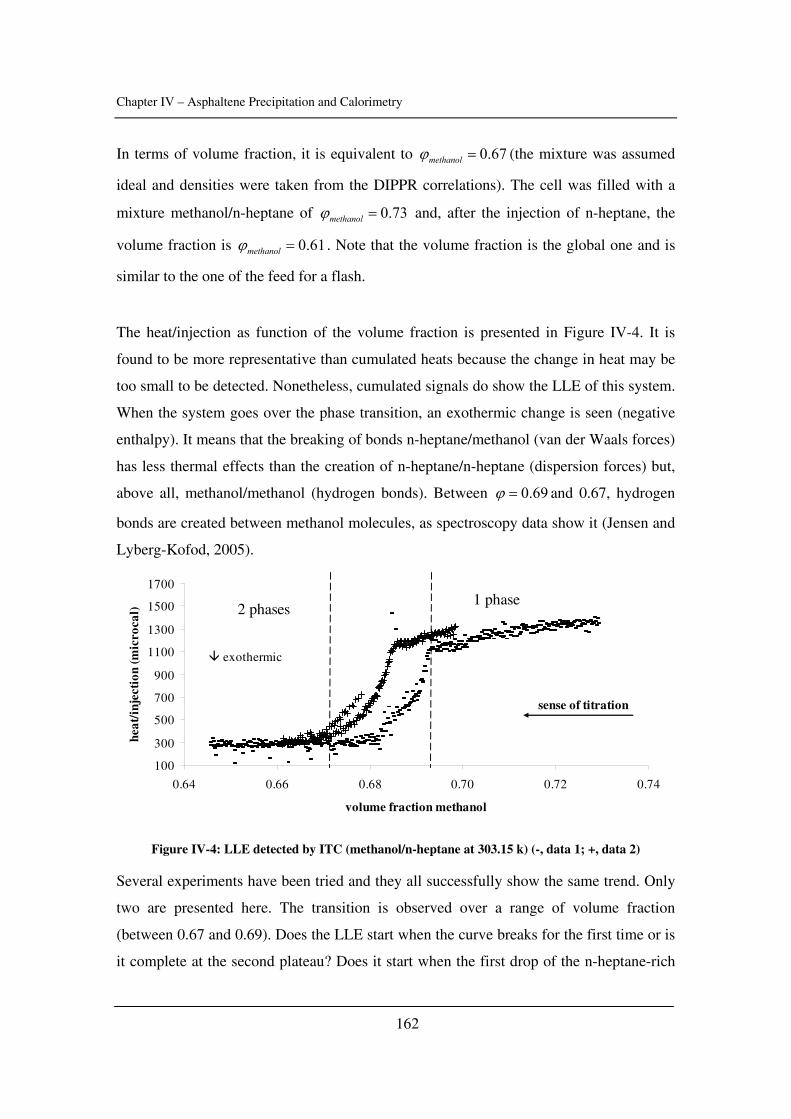
Chapter IV – Asphaltene Precipitation and Calorimetry
162
In terms of volume fraction, it is equivalent to 0.67methanolϕ = (the mixture was assumed
ideal and densities were taken from the DIPPR correlations). The cell was filled with a
mixture methanol/n-heptane of 0.73methanolϕ = and, after the injection of n-heptane, the
volume fraction is 0.61methanolϕ = . Note that the volume fraction is the global one and is
similar to the one of the feed for a flash.
The heat/injection as function of the volume fraction is presented in Figure IV-4. It is
found to be more representative than cumulated heats because the change in heat may be
too small to be detected. Nonetheless, cumulated signals do show the LLE of this system.
When the system goes over the phase transition, an exothermic change is seen (negative
enthalpy). It means that the breaking of bonds n-heptane/methanol (van der Waals forces)
has less thermal effects than the creation of n-heptane/n-heptane (dispersion forces) but,
above all, methanol/methanol (hydrogen bonds). Between 0.69ϕ = and 0.67, hydrogen
bonds are created between methanol molecules, as spectroscopy data show it (Jensen and
Lyberg-Kofod, 2005).
100
300
500
700
900
1100
1300
1500
1700
0.64 0.66 0.68 0.70 0.72 0.74
volume fraction methanol
heat
/inj
ecti
on (m
icro
cal)
1 phase2 phases
exothermic
sense of titration
Figure IV-4: LLE detected by ITC (methanol/n-heptane at 303.15 k) (-, data 1; +, data 2)
Several experiments have been tried and they all successfully show the same trend. Only
two are presented here. The transition is observed over a range of volume fraction
(between 0.67 and 0.69). Does the LLE start when the curve breaks for the first time or is
it complete at the second plateau? Does it start when the first drop of the n-heptane-rich
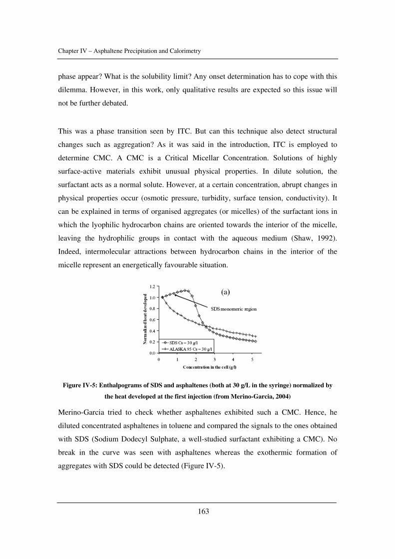
Chapter IV – Asphaltene Precipitation and Calorimetry
163
phase appear? What is the solubility limit? Any onset determination has to cope with this
dilemma. However, in this work, only qualitative results are expected so this issue will
not be further debated.
This was a phase transition seen by ITC. But can this technique also detect structural
changes such as aggregation? As it was said in the introduction, ITC is employed to
determine CMC. A CMC is a Critical Micellar Concentration. Solutions of highly
surface-active materials exhibit unusual physical properties. In dilute solution, the
surfactant acts as a normal solute. However, at a certain concentration, abrupt changes in
physical properties occur (osmotic pressure, turbidity, surface tension, conductivity). It
can be explained in terms of organised aggregates (or micelles) of the surfactant ions in
which the lyophilic hydrocarbon chains are oriented towards the interior of the micelle,
leaving the hydrophilic groups in contact with the aqueous medium (Shaw, 1992).
Indeed, intermolecular attractions between hydrocarbon chains in the interior of the
micelle represent an energetically favourable situation.
Figure IV-5: Enthalpograms of SDS and asphaltenes (both at 30 g/L in the syringe) normalized by
the heat developed at the first injection (from Merino-Garcia, 2004)
Merino-Garcia tried to check whether asphaltenes exhibited such a CMC. Hence, he
diluted concentrated asphaltenes in toluene and compared the signals to the ones obtained
with SDS (Sodium Dodecyl Sulphate, a well-studied surfactant exhibiting a CMC). No
break in the curve was seen with asphaltenes whereas the exothermic formation of
aggregates with SDS could be detected (Figure IV-5).
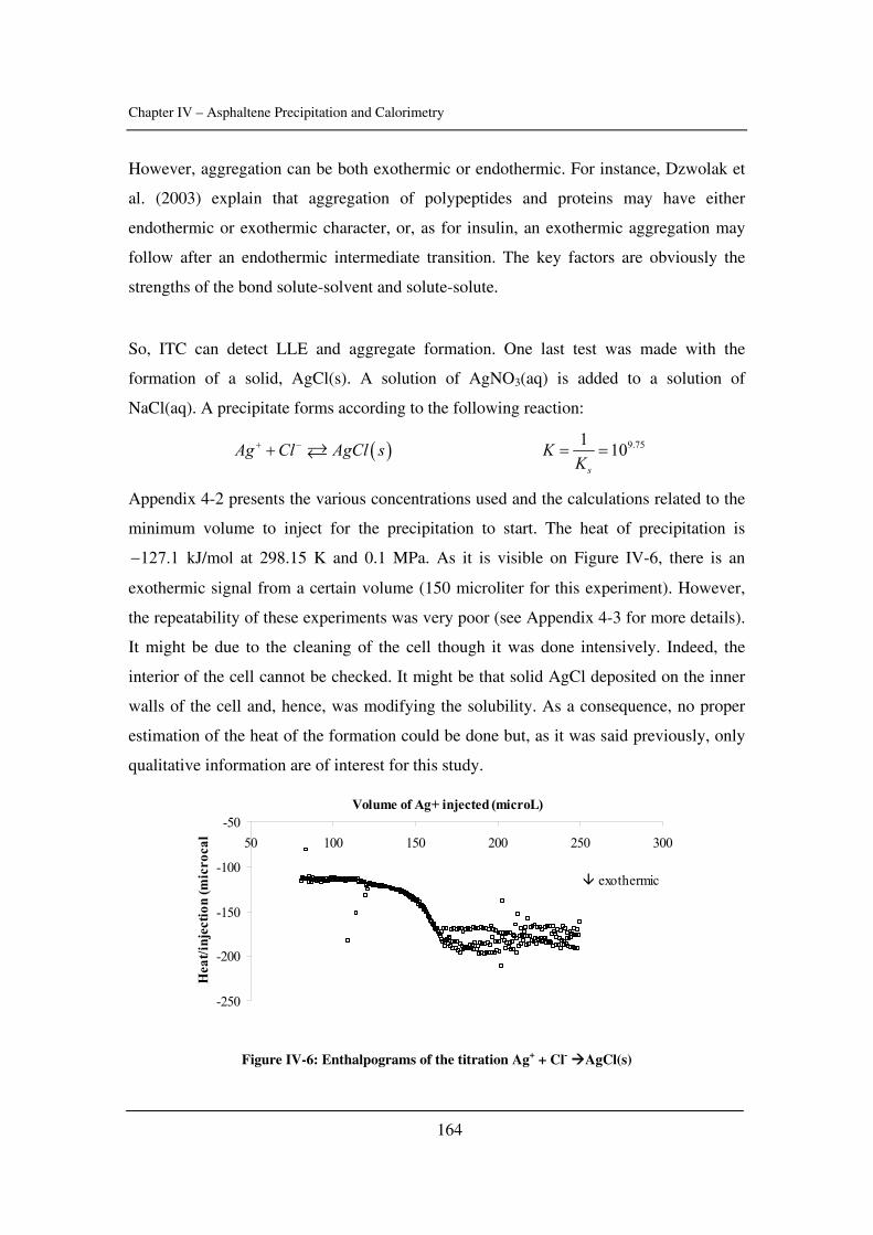
Chapter IV – Asphaltene Precipitation and Calorimetry
164
However, aggregation can be both exothermic or endothermic. For instance, Dzwolak et
al. (2003) explain that aggregation of polypeptides and proteins may have either
endothermic or exothermic character, or, as for insulin, an exothermic aggregation may
follow after an endothermic intermediate transition. The key factors are obviously the
strengths of the bond solute-solvent and solute-solute.
So, ITC can detect LLE and aggregate formation. One last test was made with the
formation of a solid, AgCl(s). A solution of AgNO3(aq) is added to a solution of
NaCl(aq). A precipitate forms according to the following reaction:
( )Ag Cl AgCl s+ −+ 9.751 10s
KK
= =
Appendix 4-2 presents the various concentrations used and the calculations related to the
minimum volume to inject for the precipitation to start. The heat of precipitation is
127.1− kJ/mol at 298.15 K and 0.1 MPa. As it is visible on Figure IV-6, there is an
exothermic signal from a certain volume (150 microliter for this experiment). However,
the repeatability of these experiments was very poor (see Appendix 4-3 for more details).
It might be due to the cleaning of the cell though it was done intensively. Indeed, the
interior of the cell cannot be checked. It might be that solid AgCl deposited on the inner
walls of the cell and, hence, was modifying the solubility. As a consequence, no proper
estimation of the heat of the formation could be done but, as it was said previously, only
qualitative information are of interest for this study.
-250
-200
-150
-100
-5050 100 150 200 250 300
Volume of Ag+ injected (microL)
Hea
t/inj
ectio
n (m
icro
cal
exothermic
Figure IV-6: Enthalpograms of the titration Ag+ + Cl- AgCl(s)
Chapter IV – Asphaltene Precipitation and Calorimetry
165
Be that as it may, it appears that ITC is able to detect some phase transitions such as LLE
or SLE and structural changes such as aggregation and CMC. But, will it be able to detect
asphaltene precipitation if the energy of the broken bonds asphaltene-solvents is
equivalent to the energy of formation asphaltenes-asphaltenes since most of them are
believed to be dispersion forces?
2.3. ITC and Asphaltene Precipitation
2.3.1. Asphaltene solutions
Asphaltene solutions in toluene were tested at different concentrations (1.4 g/L and 10
g/L) for asphaltenes extracted from a Boscan crude oil with the modified IP143 method
presented in the appendix 1.1. Onset titrations were performed at atmospheric conditions
and the onset ratio 7toluene n CV V − is 0.78. Several concentrations were tested and the onset
occurred at the same ratio toluene/n-heptane, as reported in the literature (Porte et al.,
2003).
Figure IV-7 shows the enthalpograms obtained during the titrations of the Boscan
solution with n-heptane at 303.15 K and 0.1 MPa. All the enthalpograms are presented in
Appendix IV-4. First, it is seen that the dilution of this asphaltene solution with n-alkanes
is endothermic contrary to the results obtained by Mahmoud et al. (2005). The
explanation lies in the various strengths of attractions listed in Table IV-3. The delay
between each injection was at least 300 s and the maximum injection rate was 0.8
microL/injection.
Furthermore, all the experiments showed exactly the same trend:
- Phase 1: at low n-heptane content, low noise perturbs the main signal.
- Phase 2: there is no perturbation of the signal of the dilution.
- Phase 3: much stronger disturbances appear.
The assumptions are numerous to explain such behaviour. Is phase 1 due to local
precipitation? Are the precipitated asphaltenes redissolving in zone 2? Is zone 1 due to
flocculation? Is zone 3 the “real” precipitation?
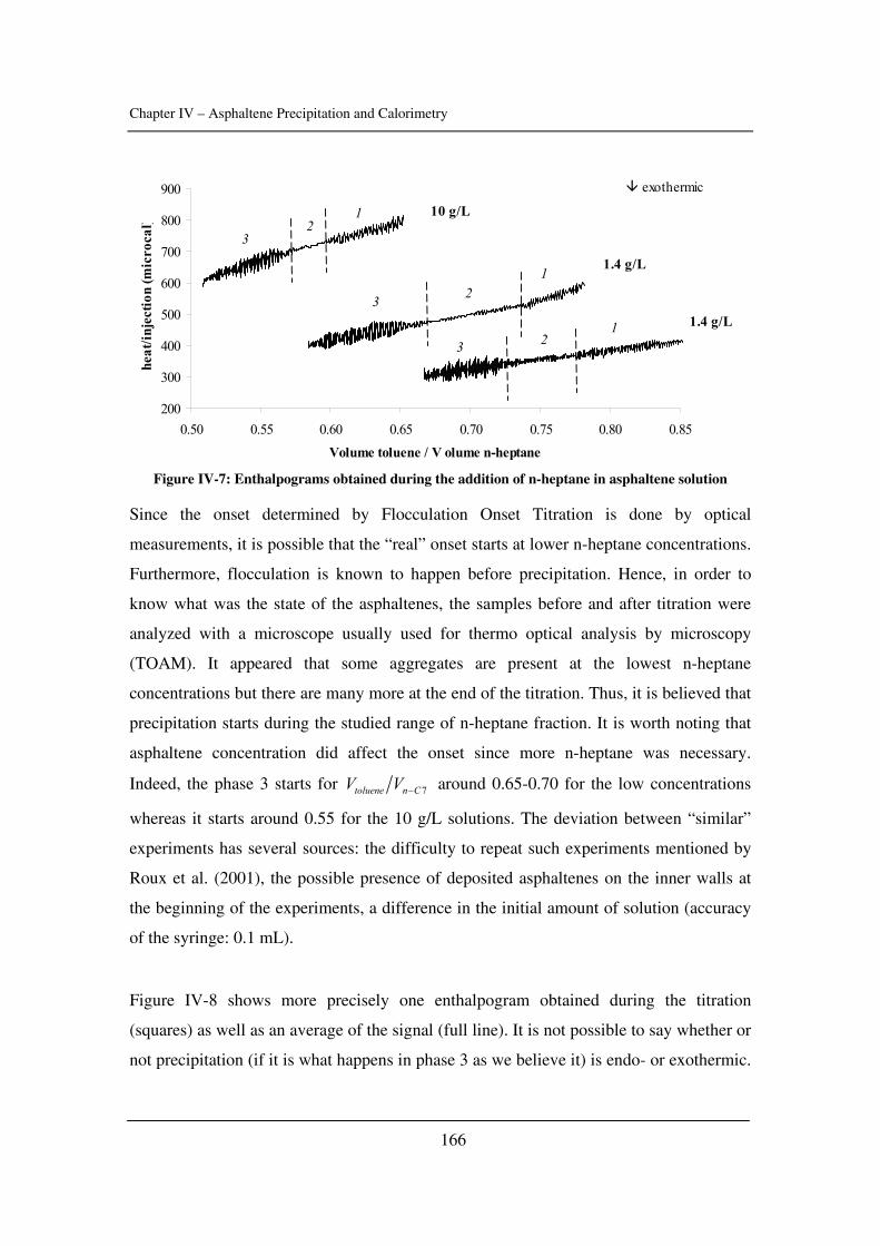
Chapter IV – Asphaltene Precipitation and Calorimetry
166
200
300
400
500
600
700
800
900
0.50 0.55 0.60 0.65 0.70 0.75 0.80 0.85Volume toluene / V olume n-heptane
heat
/inje
ctio
n (m
icro
cal)
10 g/L
1.4 g/L
1.4 g/L
12
3
1
1
2
2
3
3
exothermic
Figure IV-7: Enthalpograms obtained during the addition of n-heptane in asphaltene solution
Since the onset determined by Flocculation Onset Titration is done by optical
measurements, it is possible that the “real” onset starts at lower n-heptane concentrations.
Furthermore, flocculation is known to happen before precipitation. Hence, in order to
know what was the state of the asphaltenes, the samples before and after titration were
analyzed with a microscope usually used for thermo optical analysis by microscopy
(TOAM). It appeared that some aggregates are present at the lowest n-heptane
concentrations but there are many more at the end of the titration. Thus, it is believed that
precipitation starts during the studied range of n-heptane fraction. It is worth noting that
asphaltene concentration did affect the onset since more n-heptane was necessary.
Indeed, the phase 3 starts for 7toluene n CV V − around 0.65-0.70 for the low concentrations
whereas it starts around 0.55 for the 10 g/L solutions. The deviation between “similar”
experiments has several sources: the difficulty to repeat such experiments mentioned by
Roux et al. (2001), the possible presence of deposited asphaltenes on the inner walls at
the beginning of the experiments, a difference in the initial amount of solution (accuracy
of the syringe: 0.1 mL).
Figure IV-8 shows more precisely one enthalpogram obtained during the titration
(squares) as well as an average of the signal (full line). It is not possible to say whether or
not precipitation (if it is what happens in phase 3 as we believe it) is endo- or exothermic.
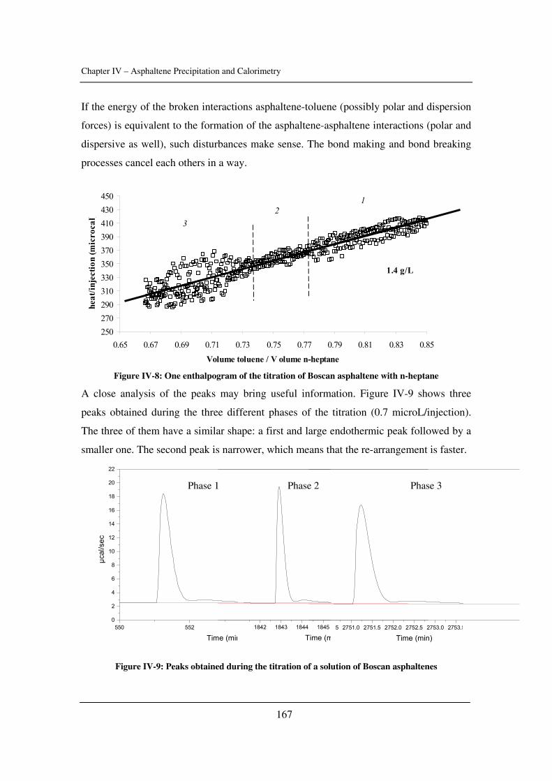
Chapter IV – Asphaltene Precipitation and Calorimetry
167
If the energy of the broken interactions asphaltene-toluene (possibly polar and dispersion
forces) is equivalent to the formation of the asphaltene-asphaltene interactions (polar and
dispersive as well), such disturbances make sense. The bond making and bond breaking
processes cancel each others in a way.
250270290310330350370390410430450
0.65 0.67 0.69 0.71 0.73 0.75 0.77 0.79 0.81 0.83 0.85Volume toluene / V olume n-heptane
heat
/inje
ctio
n (m
icro
cal)
1.4 g/L
1
32
Figure IV-8: One enthalpogram of the titration of Boscan asphaltene with n-heptane
A close analysis of the peaks may bring useful information. Figure IV-9 shows three
peaks obtained during the three different phases of the titration (0.7 microL/injection).
The three of them have a similar shape: a first and large endothermic peak followed by a
smaller one. The second peak is narrower, which means that the re-arrangement is faster.
1842 1843 1844 1845
Time (m550 552
0
2
4
6
8
10
12
14
16
18
20
22
Time (min
µcal
/sec
5 2751.0 2751.5 2752.0 2752.5 2753.0 2753.5
Time (min)
Phase 1 Phase 2 Phase 3
Figure IV-9: Peaks obtained during the titration of a solution of Boscan asphaltenes
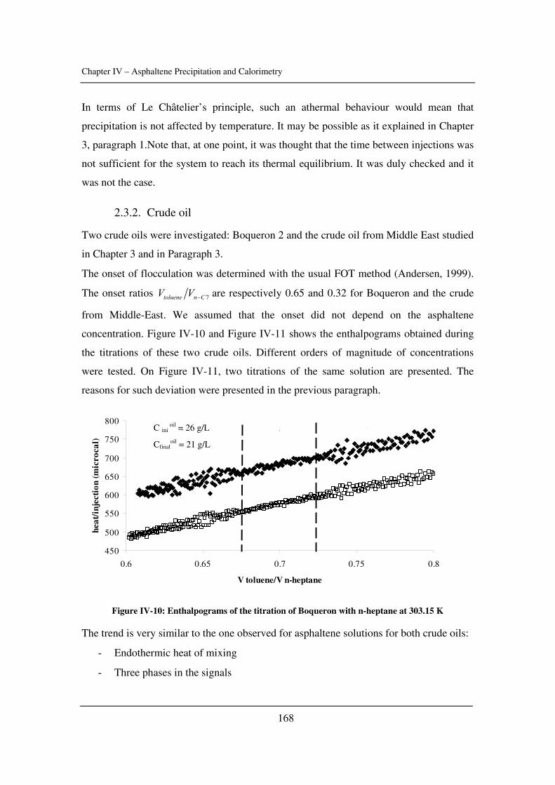
Chapter IV – Asphaltene Precipitation and Calorimetry
168
In terms of Le Châtelier’s principle, such an athermal behaviour would mean that
precipitation is not affected by temperature. It may be possible as it explained in Chapter
3, paragraph 1.Note that, at one point, it was thought that the time between injections was
not sufficient for the system to reach its thermal equilibrium. It was duly checked and it
was not the case.
2.3.2. Crude oil
Two crude oils were investigated: Boqueron 2 and the crude oil from Middle East studied
in Chapter 3 and in Paragraph 3.
The onset of flocculation was determined with the usual FOT method (Andersen, 1999).
The onset ratios 7toluene n CV V − are respectively 0.65 and 0.32 for Boqueron and the crude
from Middle-East. We assumed that the onset did not depend on the asphaltene
concentration. Figure IV-10 and Figure IV-11 shows the enthalpograms obtained during
the titrations of these two crude oils. Different orders of magnitude of concentrations
were tested. On Figure IV-11, two titrations of the same solution are presented. The
reasons for such deviation were presented in the previous paragraph.
450
500
550
600
650
700
750
800
0.6 0.65 0.7 0.75 0.8
V toluene/V n-heptane
heat
/inj
ecti
on (m
icro
cal)
123
Figure IV-10: Enthalpograms of the titration of Boqueron with n-heptane at 303.15 K
The trend is very similar to the one observed for asphaltene solutions for both crude oils:
- Endothermic heat of mixing
- Three phases in the signals
C ini oil = 26 g/L
Cfinaloil = 21 g/L
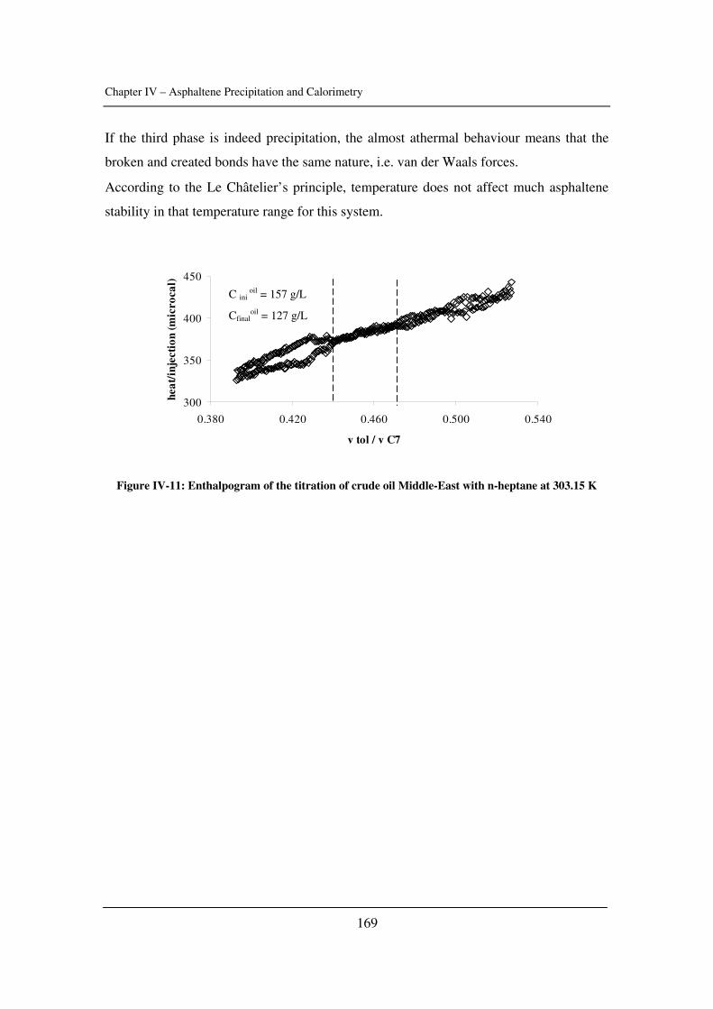
Chapter IV – Asphaltene Precipitation and Calorimetry
169
If the third phase is indeed precipitation, the almost athermal behaviour means that the
broken and created bonds have the same nature, i.e. van der Waals forces.
According to the Le Châtelier’s principle, temperature does not affect much asphaltene
stability in that temperature range for this system.
300
350
400
450
0.380 0.420 0.460 0.500 0.540
v tol / v C7
heat
/inj
ecti
on (m
icro
cal)
Figure IV-11: Enthalpogram of the titration of crude oil Middle-East with n-heptane at 303.15 K
C ini oil = 157 g/L
Cfinaloil = 127 g/L
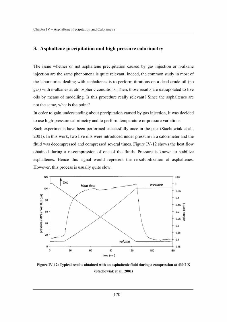
Chapter IV – Asphaltene Precipitation and Calorimetry
170
3. Asphaltene precipitation and high pressure calorimetry
The issue whether or not asphaltene precipitation caused by gas injection or n-alkane
injection are the same phenomena is quite relevant. Indeed, the common study in most of
the laboratories dealing with asphaltenes is to perform titrations on a dead crude oil (no
gas) with n-alkanes at atmospheric conditions. Then, those results are extrapolated to live
oils by means of modelling. Is this procedure really relevant? Since the asphaltenes are
not the same, what is the point?
In order to gain understanding about precipitation caused by gas injection, it was decided
to use high-pressure calorimetry and to perform temperature or pressure variations.
Such experiments have been performed successfully once in the past (Stachowiak et al.,
2001). In this work, two live oils were introduced under pressure in a calorimeter and the
fluid was decompressed and compressed several times. Figure IV-12 shows the heat flow
obtained during a re-compression of one of the fluids. Pressure is known to stabilize
asphaltenes. Hence this signal would represent the re-solubilization of asphaltenes.
However, this process is usually quite slow.
Figure IV-12: Typical results obtained with an asphaltenic fluid during a compression at 430.7 K
(Stachowiak et al., 2001)
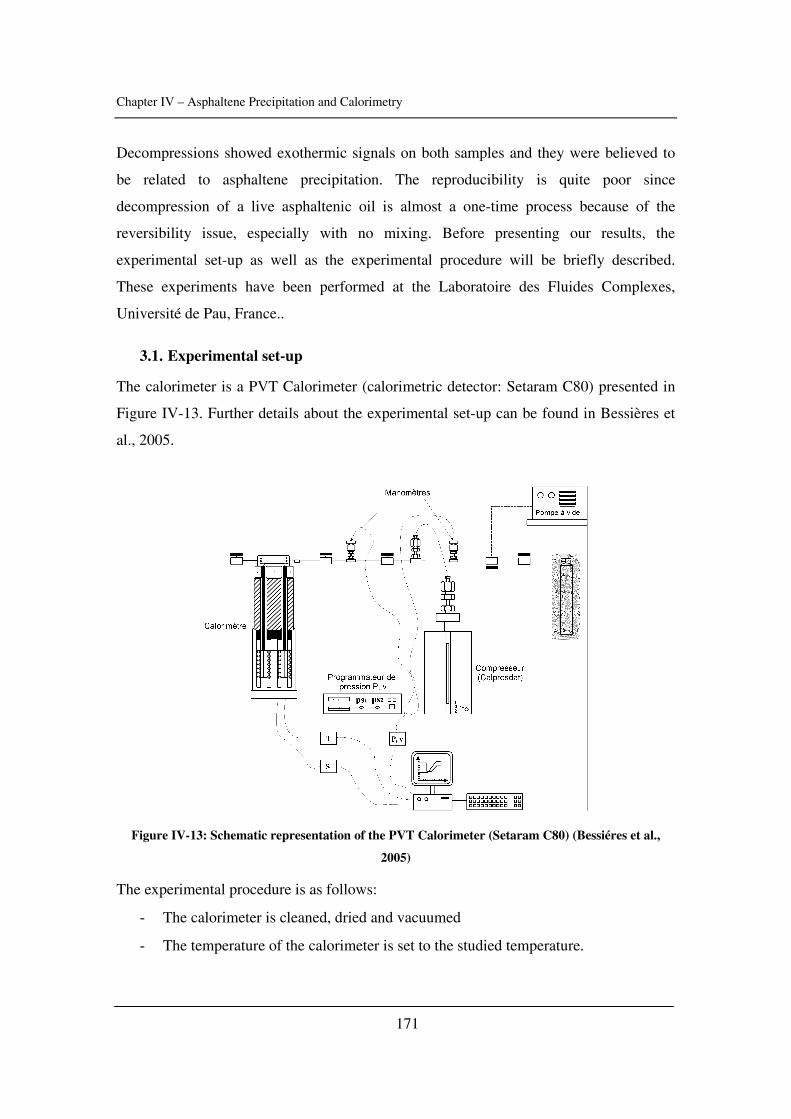
Chapter IV – Asphaltene Precipitation and Calorimetry
171
Decompressions showed exothermic signals on both samples and they were believed to
be related to asphaltene precipitation. The reproducibility is quite poor since
decompression of a live asphaltenic oil is almost a one-time process because of the
reversibility issue, especially with no mixing. Before presenting our results, the
experimental set-up as well as the experimental procedure will be briefly described.
These experiments have been performed at the Laboratoire des Fluides Complexes,
Université de Pau, France..
3.1. Experimental set-up
The calorimeter is a PVT Calorimeter (calorimetric detector: Setaram C80) presented in
Figure IV-13. Further details about the experimental set-up can be found in Bessières et
al., 2005.
Figure IV-13: Schematic representation of the PVT Calorimeter (Setaram C80) (Bessiéres et al.,
2005)
The experimental procedure is as follows:
- The calorimeter is cleaned, dried and vacuumed
- The temperature of the calorimeter is set to the studied temperature.
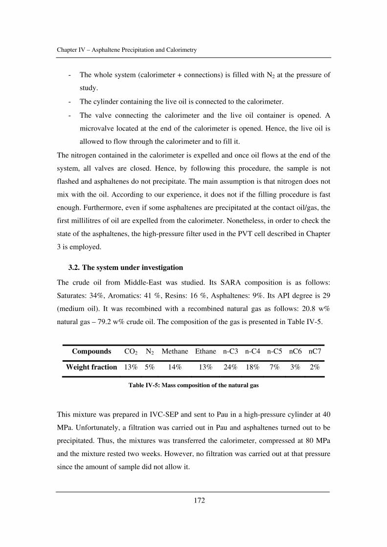
Chapter IV – Asphaltene Precipitation and Calorimetry
172
- The whole system (calorimeter + connections) is filled with N2 at the pressure of
study.
- The cylinder containing the live oil is connected to the calorimeter.
- The valve connecting the calorimeter and the live oil container is opened. A
microvalve located at the end of the calorimeter is opened. Hence, the live oil is
allowed to flow through the calorimeter and to fill it.
The nitrogen contained in the calorimeter is expelled and once oil flows at the end of the
system, all valves are closed. Hence, by following this procedure, the sample is not
flashed and asphaltenes do not precipitate. The main assumption is that nitrogen does not
mix with the oil. According to our experience, it does not if the filling procedure is fast
enough. Furthermore, even if some asphaltenes are precipitated at the contact oil/gas, the
first millilitres of oil are expelled from the calorimeter. Nonetheless, in order to check the
state of the asphaltenes, the high-pressure filter used in the PVT cell described in Chapter
3 is employed.
3.2. The system under investigation
The crude oil from Middle-East was studied. Its SARA composition is as follows:
Saturates: 34%, Aromatics: 41 %, Resins: 16 %, Asphaltenes: 9%. Its API degree is 29
(medium oil). It was recombined with a recombined natural gas as follows: 20.8 w%
natural gas – 79.2 w% crude oil. The composition of the gas is presented in Table IV-5.
Compounds CO2 N2 Methane Ethane n-C3 n-C4 n-C5 nC6 nC7
Weight fraction 13% 5% 14% 13% 24% 18% 7% 3% 2%
Table IV-5: Mass composition of the natural gas
This mixture was prepared in IVC-SEP and sent to Pau in a high-pressure cylinder at 40
MPa. Unfortunately, a filtration was carried out in Pau and asphaltenes turned out to be
precipitated. Thus, the mixtures was transferred the calorimeter, compressed at 80 MPa
and the mixture rested two weeks. However, no filtration was carried out at that pressure
since the amount of sample did not allow it.
Chapter IV – Asphaltene Precipitation and Calorimetry
173
3.3. Variations of temperature
The first series of experiments was a temperature scanning between 30 and 90°C at 80
MPa with the smallest temperature rate possible with this calorimeter (0.05 °C/min). The
volumetric and calorimetric signals are recorded simultaneously. The first experiment
showed variations in both signals around 350 K: an increase in thermal expansivity (the
slope of volume with respect to temperature) and an exothermic signal (Figure IV-14).
250260270280290300310320330340350
300 310 320 330 340 350 360 370
T (K)
calo
rim
etri
c si
gnal
(a.u
.)
0
0.1
0.2
0.3
0.4
delta
vol
ume
(mL
volume
calorimetric signal
exothermic
Figure IV-14: Volumetric and calorimetric signals during the first temperature variation at 80 MPa
(system: crude oil from Middle-East recombined 20.8w% of natural gas)
The phase transition is believed to be a precipitation since there is a “gain in volume”
(about 0.1 mL for a total volume of 30 mL). An exothermic precipitation means that
temperature would stabilize asphaltenes. On the contrary, asphaltenes seem to precipitate
with an increase of temperature. So, is the Le Châtelier’s principle not used properly or is
it the understanding of the experimental results? No filtration was carried out but the gain
in volume gives to understand that a new phase is created. As for the Le Châtelier’s
principle, as it was said in Chapter 3, paragraph 1.4, only one equilibrium was taken into
account. Could it be that the other reactions are not negligible as it was assumed?
Before 350 K, the signal is slightly perturbed. It might be that flocculation – which
precedes precipitation – affects the calorimetric signal since it is change in the state of
aggregation. Nonetheless, since both volumetric and calorimetric signals exhibit strong
variations at the same temperature, the phase transition is believed to happen at 350 K.
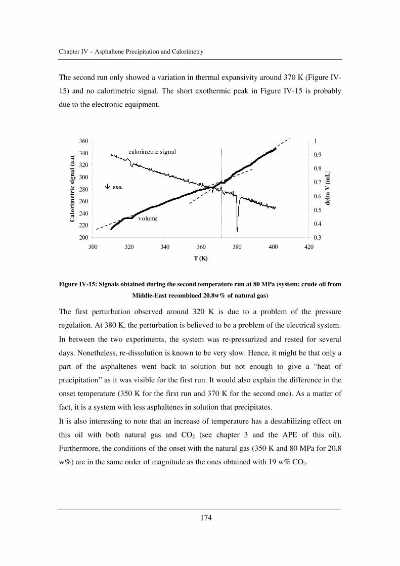
Chapter IV – Asphaltene Precipitation and Calorimetry
174
The second run only showed a variation in thermal expansivity around 370 K (Figure IV-
15) and no calorimetric signal. The short exothermic peak in Figure IV-15 is probably
due to the electronic equipment.
200
220
240
260
280
300
320
340
360
300 320 340 360 380 400 420
T (K)
Cal
orim
etri
c si
gnal
(a.u
)
0.3
0.4
0.5
0.6
0.7
0.8
0.9
1
delta
V (m
L)
calorimetric signal
volume
exo.
Figure IV-15: Signals obtained during the second temperature run at 80 MPa (system: crude oil from
Middle-East recombined 20.8w% of natural gas)
The first perturbation observed around 320 K is due to a problem of the pressure
regulation. At 380 K, the perturbation is believed to be a problem of the electrical system.
In between the two experiments, the system was re-pressurized and rested for several
days. Nonetheless, re-dissolution is known to be very slow. Hence, it might be that only a
part of the asphaltenes went back to solution but not enough to give a “heat of
precipitation” as it was visible for the first run. It would also explain the difference in the
onset temperature (350 K for the first run and 370 K for the second one). As a matter of
fact, it is a system with less asphaltenes in solution that precipitates.
It is also interesting to note that an increase of temperature has a destabilizing effect on
this oil with both natural gas and CO2 (see chapter 3 and the APE of this oil).
Furthermore, the conditions of the onset with the natural gas (350 K and 80 MPa for 20.8
w%) are in the same order of magnitude as the ones obtained with 19 w% CO2.
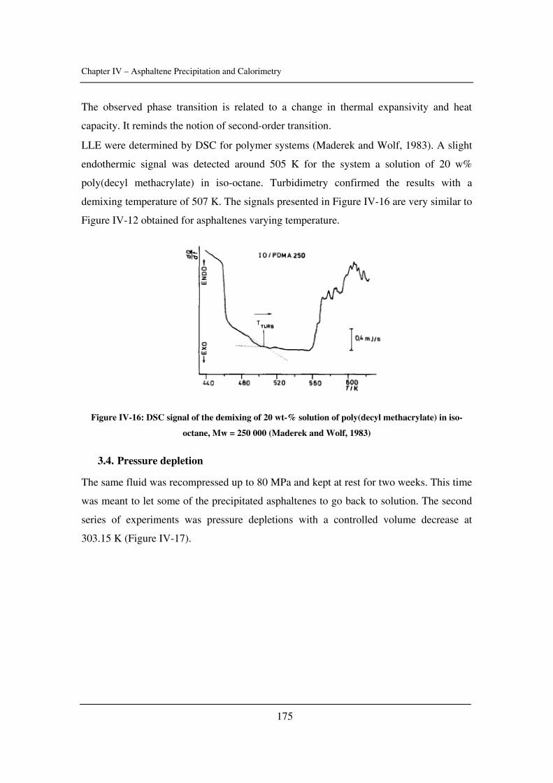
Chapter IV – Asphaltene Precipitation and Calorimetry
175
The observed phase transition is related to a change in thermal expansivity and heat
capacity. It reminds the notion of second-order transition.
LLE were determined by DSC for polymer systems (Maderek and Wolf, 1983). A slight
endothermic signal was detected around 505 K for the system a solution of 20 w%
poly(decyl methacrylate) in iso-octane. Turbidimetry confirmed the results with a
demixing temperature of 507 K. The signals presented in Figure IV-16 are very similar to
Figure IV-12 obtained for asphaltenes varying temperature.
Figure IV-16: DSC signal of the demixing of 20 wt-% solution of poly(decyl methacrylate) in iso-
octane, Mw = 250 000 (Maderek and Wolf, 1983)
3.4. Pressure depletion
The same fluid was recompressed up to 80 MPa and kept at rest for two weeks. This time
was meant to let some of the precipitated asphaltenes to go back to solution. The second
series of experiments was pressure depletions with a controlled volume decrease at
303.15 K (Figure IV-17).
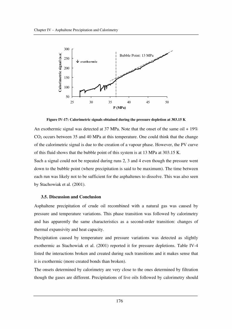
Chapter IV – Asphaltene Precipitation and Calorimetry
176
50
100
150
200
250
300
25 30 35 40 45 50P (MPa)
Cal
orim
etri
c si
gnal
(a.u
) exothermic
Figure IV-17: Calorimetric signals obtained during the pressure depletion at 303.15 K
An exothermic signal was detected at 37 MPa. Note that the onset of the same oil + 19%
CO2 occurs between 35 and 40 MPa at this temperature. One could think that the change
of the calorimetric signal is due to the creation of a vapour phase. However, the PV curve
of this fluid shows that the bubble point of this system is at 13 MPa at 303.15 K.
Such a signal could not be repeated during runs 2, 3 and 4 even though the pressure went
down to the bubble point (where precipitation is said to be maximum). The time between
each run was likely not to be sufficient for the asphaltenes to dissolve. This was also seen
by Stachowiak et al. (2001).
3.5. Discussion and Conclusion
Asphaltene precipitation of crude oil recombined with a natural gas was caused by
pressure and temperature variations. This phase transition was followed by calorimetry
and has apparently the same characteristics as a second-order transition: changes of
thermal expansivity and heat capacity.
Precipitation caused by temperature and pressure variations was detected as slightly
exothermic as Stachowiak et al. (2001) reported it for pressure depletions. Table IV-4
listed the interactions broken and created during such transitions and it makes sense that
it is exothermic (more created bonds than broken).
The onsets determined by calorimetry are very close to the ones determined by filtration
though the gases are different. Precipitations of live oils followed by calorimetry should
Bubble Point: 13 MPa

Chapter IV – Asphaltene Precipitation and Calorimetry
177
be combined with filtration to be sure of the obtained signals. But, it would mean that
each sample could only be used once and recombination is quite heavy and time-
consuming. Furthermore, the amount of available crude oil did not allow it.
Hence, with enough crude oil, a complete APE (Asphaltene Phase Envelope) including
onset and bubble points could be determined thanks to HP calorimetry. Indeed, bubble
points can be determined by calorimetry (Verdier et al., 2005).
Chapter IV – Asphaltene Precipitation and Calorimetry
178
4. Conclusion about calorimetry
Two asphaltene precipitations were tested: the one induced by n-alkanes and the one due
to gas and variations of T and P .
The first one did not exhibit any strong exothermic or endothermic signals but
precipitation was rather athermal contrary to what has been observed for model systems
(LLE, SLE, micellization). Therefore, it appears the energy of the broken bonds is
balanced by the energy of the created ones. The n-heptane content was increased but no
difference was observed. The enthalpograms of the crude oils were similar to the ones of
the asphaltene solutions.
The second series of tests was performed with HP calorimeter and recombined oils. Both
pressure depletions and temperature variations induced asphaltene precipitations. The
increase in volume confirms these results but no filtration was performed. The re-
dissolution of asphaltenes was very slow and was not seen. Hence, such experiments can
be performed once. An accurate high-pressure pycnometer would enable the onset
determination without the difficult of calorimetry.
Chapter IV – Asphaltene Precipitation and Calorimetry
179
Literature
Andersen S.I., Birdi K.S., Aggregation of asphaltenes as determined by calorimetry, J. Coll. Int. Sci. (1991), 142, 497 – 502 Andersen S.I., Christensen S.D., The critical micelle concentration of asphaltenes as measured by calorimetry, Energ. Fuel (2000), 14, 38-42 Andersen S.I., del Rio J.M., Khvostitchenko D., Shakir S., Lira-Galeana C., Interaction and solubilization of water by petroleum asphaltenes in organic solution, Langmuir (2001), 17, 307 – 313 Bessieres D., Saint-Guirons H, Daridon J.-L., J. Therm. Anal. Calorim. (1999), 58, 39-49 Bessières D., Lafitte T., Daridon J.-L., Randzio S., High pressure thermal expansion of gases: Measurements and calibration, Thermochim. Acta (2005), 428, 25-30 Dzwolak W., Ravindra, R., Lendermann J. Winter R., Aggregation of bovine insulin probed by DSC/PPC calorimetry and FTIR spectroscopy, Biochemistry (2003), 42, 11347-11355 Ekulu G., Nicolas C., Achard C., Rogalski M., Characterization of aggregation processes in crude oils using differential scanning calorimetry, Energ. Fuel. (2005), 19, 1297-1302 Fenistein D., Barré L., Broseta D., Espinat D., Livet A., Roux J.N., Scarsella M., Viscosimetric and neutron scattering study of asphaltene aggregates in mixed toluene/heptane solvents, Langmuir (1998), 14, 1013 – 1020 Hotier G., Robin M., Action de divers diluants sur les produits pétroliers lourds : mesure, interprétation et prévision de la floculation des asphaltenes, Rev. I. Fr. Petrol. (1983), 38, 101 – 120 Jensen L., Lyberg-Kofod J., Investigation of Hydrogen bonding in Associating Compounds Using IR Spectroscopy, Midterm Project, Department of Chemical Engineering, Technical University of Denmark, January 2005 Lundberg G. W., Thermodynamics of Solutions, XI. Heats of Mixing of Hydrocarbons, J. Chem. Eng. Data (1964), 9, 193-198 Maderek E., Wolf B.A., Detection of liquid-liquid demixing by differential scanning calorimetry, Polym. Bull. (1983), 10, 458 - 463 Mahmoud R., PhD Thesis, Nancy, 1999
Chapter IV – Asphaltene Precipitation and Calorimetry
180
Mahmoud R., Gierycz P., Solimando R., Rogalski M., Calorimetic probing of n-alkane-petroleum asphaltene interactions, Energ. Fuel. (2005), 19, 2474 - 2479 Merino-Garcia D., Calorimetric investigations of asphaltene self-association and interaction with resins, Ph.D. Thesis, IVC-SEP, Department of Chemical Engineering, Denmark, Technical University, Lyngby, Denmark, 2004 Porte G., Zhou H., Lazzeri V., Reversible description of asphaltene colloidal association and precipitation, Langmuir (2003), 19, 40 – 47 Roux J.N., Broseta D., Demé B., SANS study of asphaltene aggregation: concentration and solvent quality effects, Langmuir (2001), 17, 5085 – 5092 Shaw D.J., Introduction to colloid and surface chemistry, 4th edition, Butterworth-Heinemann Publications, 1992 Sirota E.B., Physical structure of asphaltenes, Energ. Fuel. (2005), 19, 1290-1296 Stachowiak L., Diagrammes de phases : fluides supercritiques-hydrocarbures lourds. Etudes des phénomènes de floculation des fluides asphalténiques, PhD Thesis, Clermont-Ferrand, 2001 Stachowiak Ch., Grolier J.-P. E., Randzio S.L., Transitiometric investigation of asphaltenic fluids under in-well pressure and temperature conditions, Energ. Fuel. (2001), 15, 1033 – 1037 Stachowiak C., Viguié J.R., JPE Grolier, Rogalski M., Effetc of n-alkanes on asphaltene structuring in Petroleum Oils, Langmuir (2005), 21, 4821 – 4829 Sørensen J.M., Arlt W., Liquid-liquid equilibrium data collection, Binary Systems, Chemistry Data Series, vol. V, Part 1, Dechema, Frankfurt, 1995 Verdier S., Duong D., Andersen S.I., Experimental determination of solubility parameters of oils as a function of pressure, Energ. Fuel. (2005), 19, 1225 - 1229 Zhang Y., Takanohashi T., Sato S., Saito I., Observation of glass transition in asphaltenes, Energ. Fuel. (2004), 18, 283 - 284 Zhang Y., Takanohashi T., Shishido T., Sato S., Saito I., Estimating the interaction energy of asphaltene aggregates with aromatic solvents, Energ. Fuel. (2005), 19, 1023 – 1028
Chapter V – Modelling of Asphaltene Precipitation
181
Chapter V
Modelling of Asphaltene Precipitation
Chapter V – Modelling of Asphaltene Precipitation
182
Table of Contents
1. The different families of models .......................................................................... 185
1.1. The steric-stabilization model......................................................................... 185
1.2. The thermodynamic models............................................................................ 187
1.2.1. The Flory-Huggins equation ................................................................... 187
1.2.2. The Scatchard-Hildebrand equation ....................................................... 193
1.2.3. The Scott-Magat equation....................................................................... 193
1.2.4. Cubic equations of state .......................................................................... 194
1.2.5. The association EOS............................................................................... 195
1.3. Scaling equations ............................................................................................ 197
1.4. Conclusion ...................................................................................................... 197
2. Asphaltene precipitation and cubic EOS............................................................ 198
2.1. The model ....................................................................................................... 198
2.2. The dilution effect........................................................................................... 198
2.3. Phase envelopes .............................................................................................. 199
2.4. Volumetric calculations .................................................................................. 201
2.5. Gas injection ................................................................................................... 202
3. A new approach combining aggregation and cubic EOS.................................. 206
3.1. The TOTAL model ......................................................................................... 206
3.2. Consistency tests............................................................................................. 211
3.3. A second approach: the aggregation model .................................................... 213
3.3.1. The dilution effect................................................................................... 214
3.3.2. Phase envelopes ...................................................................................... 216
3.3.3. Gas injection ........................................................................................... 217
3.3.4. Conclusion about the aggregation model................................................ 221

Chapter V – Modelling of Asphaltene Precipitation
183
4. Conclusion ............................................................................................................. 223
Literature....................................................................................................................... 224
List of symbols............................................................................................................... 227
Chapter V – Modelling of Asphaltene Precipitation
184
The petroleum industry needs models to predict asphaltene precipitation. However, a
dilemma arises: asphaltenic fluids are complex and need complex models to be described,
i.e. they require many parameters and the more parameters, the more fitting procedures
are necessary. Furthermore, although models are able to describe asphaltene phase
envelopes, prediction remains a chimera out of reach so far. Nonetheless, all these efforts
done through the years helped shaping the experimental research about asphaltenes,
pointing out which characteristics were necessary (molecular weight, solubility
parameters and critical parameters for example).
Though the understanding of asphaltene precipitation is relatively poor, a lot of efforts
have been put into modelling since it is much less cost-dissuasive than experiments,
especially at high pressure and temperature conditions. The modelling of asphaltenic
fluids followed the evolution of thermodynamics, starting with the simple solubility
parameters and the regular solutions and ending up with various versions of SAFT
nowadays. Most of the papers dealing with asphaltene modelling claim that they
successfully described experimental results. Obviously, it is not the case. The
determination of input parameters remains the key issue to move from the description
phase to the prediction one.
In this chapter, the various models used over the years will be briefly presented. Then,
examples of phase equilibria calculations with a cubic equation of state will be shown for
asphaltenic systems in order to evaluate the influence of the input parameters. Finally, a
model developed by Total will be presented. This model takes into account aggregation
and modifies fugacities. A second approach - based on the same assumptions but
modifying the a and b parameters of asphaltenes - will also be introduced and some
results will be shown.
Chapter V – Modelling of Asphaltene Precipitation
185
1. The different families of models
Asphaltenes are said to be either peptized by resins or solvated by the liquid medium.
Hence, two families of models exist in the literature (Cimino et al., 1995):
- The lyophobic models: asphaltenes are lyophobic colloids (solvent-hating). They
are peptized by resins and the dispersion is a two-phase system. This co-called
“colloidal model” has strongly influenced the way of thinking of scientists since
Nellesteyn, Pfeiffer and Saal claimed that asphaltenes were micelles composed of
an insoluble, aromatic core with adsorbed resin molecules, providing steric
stabilization and thereby preventing flocculation and precipitation. This
description of the asphaltene also implies that asphaltene precipitation is
irreversible.
- The lyophilic models: asphaltenes are lyophilic colloids (solvent-loving)
surrounded and solvated by the liquid medium. It is a true solution, hence
reversible. In this model, asphaltene monomers and aggregates are in
thermodynamic equilibrium. The role of resins on the stabilization is due to their
influence on the solvation power of the liquid medium. Destabilization occurs
when the solvation power of the liquid medium is too poor.
These models will be discussed now as well as their various versions.
1.1. The steric-stabilization model
Leontaritis and Mansoori mainly developed this model (Leontaritis and Manssori, 1987).
They used the picture promoted by Nellensteyn, i.e. that asphaltenes are insoluble, solid
particles peptized by resins adsorbed onto their surfaces.
According to them, the asphaltene fraction is stable when the chemical potential of resins
2μΔ is lower than a critical one 2CRμΔ . 2μΔ is expressed as follows:
( )( ) ( )22 2 2 2ln 1 1 1RT r rμ ϕ ϕ χ ϕ⎡ ⎤Δ = − − − + −⎣ ⎦ Eq V-1
Chapter V – Modelling of Asphaltene Precipitation
186
where 2μΔ is the difference between the chemical potentials of the resins in solution and
in their reference state, R the gas constant, T the temperature, 2ϕ the volume fraction of
the resins, χ the interaction parameter between resins and solvents and r the ratio
between the molar volumes of the resins and the solvent.
The critical chemical potential 2CRμΔ refers to the value when the number of resins
adsorbed on the surface of the asphaltene aggregates is the minimum required for their
peptization.
This model has been further developed but it has only been employed for data regression.
Furthermore, the concepts behind this model still need to be proved: are resins physically
present at the interface between the asphaltene micelles and the crude oil? Isolated
asphaltene fractions can be stable in some solvents. Hence, it emphasizes that the
presence of resins is not a necessary condition for the stabilization of asphaltene
aggregates (Cimino et al., 1995). The reversibility – discussed in Chapter 1 paragraph
1.6.3. - does not support this model neither.
Victorov and Firoozabadi developed a micellization model: it uses the “Nellensteyn
assumptions”, like the previous model (Victorov and Firoozabadi, 1996). Three major
contributions to the process of micelle formation are taken into account:
- The lyophobic contributions: they represent the free energy gain upon
transferring asphaltene and resin molecules from an indefinitely diluted crude to a
micelle.
- The interfacial contribution: a definite positive interfacial tension is attributed
to the micellar core in the crude
- The electrostatic contribution
The Peng-Robinson EOS was used to describe the properties of the bulk-phase. Some of
the parameters were estimated and some fitted. The model was able to describe the
asphaltene precipitation but with a low degree of accuracy. Furthermore, the issue of
reversibility was not discussed. This approach was further investigated by Fahim and co-
workers who used a group-contribution method to estimate the critical properties of the
Chapter V – Modelling of Asphaltene Precipitation
187
asphaltenes, resins and oil (Fahim et al., 2001). The amount of precipitated asphaltenes
was predicted within 0.57% according to the authors, which seems even better than the
experimental accuracy of such experiments.
So, as tempting as this model can appear, it seems quite unlikely to be able to describe or
predict asphaltene precipitation properly since it has not be proved so far.
1.2. The thermodynamic models
1.2.1. The Flory-Huggins equation
The first model treating asphaltenes as solvated in a liquid medium was the Flory theory
for polymer solutions. This method decouples the vapour-liquid equilibrium from the
liquid-solid one. The vapour-liquid calculations are first done and then a correction is
applied to the liquid phase accounting that the vapour phase remains unchanged.
Hirschberg and co-workers treated asphaltenes as monodispersed solvated
macromolecules without considering resins especially but only as a part of the solvent
(Hirschberg et al., 1984). After several simplifications, the maximum volume fraction of
soluble asphaltenes in the crude maxaϕ was expressed as follows:
( )2max exp 1a l la a l
l a
v v vv v RT
ϕ δ δ⎡ ⎤⎛ ⎞
= − − −⎢ ⎥⎜ ⎟⎝ ⎠⎣ ⎦
Eq V-2
where v is the molar volume, δ the solubility parameter, R the gas constant and T the
temperature. The subscripts a and l respectively refer to the asphaltenes and the liquid
medium.
The solubility parameter of the liquid was calculated with the SRK EOS after the fluid
was characterized. The asphaltene properties were estimated from titration experiments.
The work they achieved is quite impressive since the effects of pressure, gas injection
and temperature were investigated. This is the reason why this work remains as a
reference.
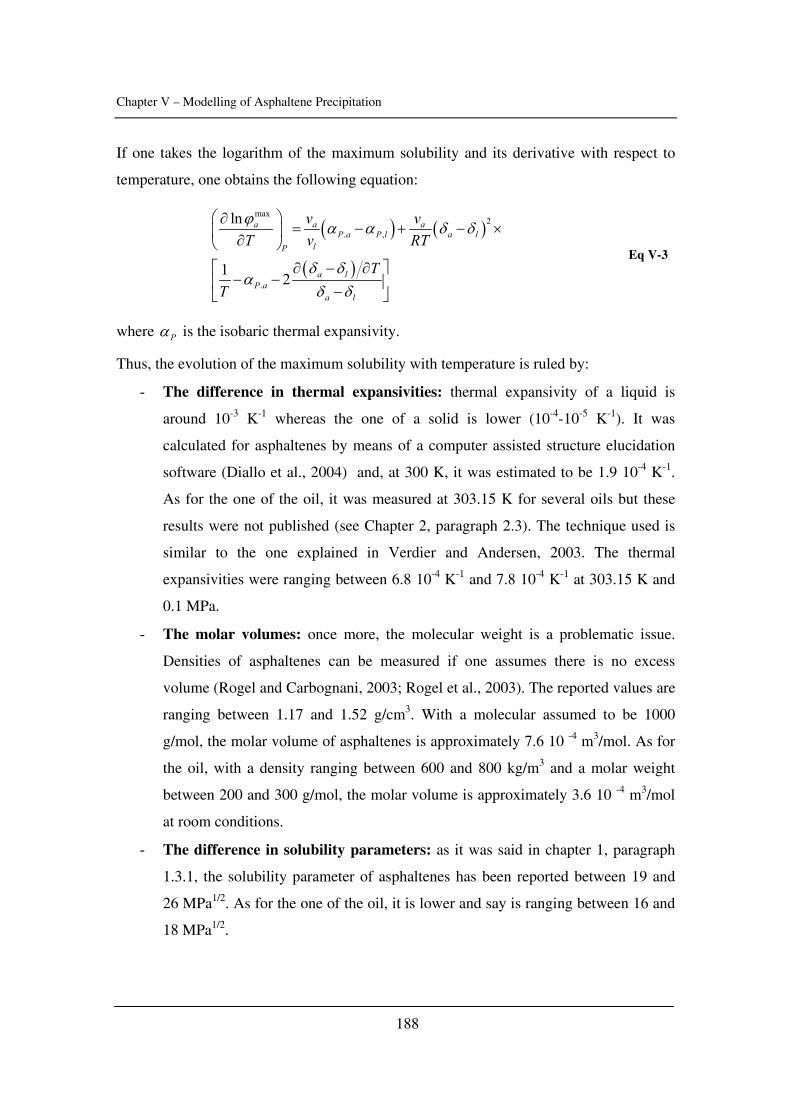
Chapter V – Modelling of Asphaltene Precipitation
188
If one takes the logarithm of the maximum solubility and its derivative with respect to
temperature, one obtains the following equation:
( ) ( )
( )
max2
. ,
.
ln
1 2
a a aP a P l a l
lP
a lP a
a l
v vT v RT
TT
ϕ α α δ δ
δ δα
δ δ
⎛ ⎞∂= − + − ×⎜ ⎟∂⎝ ⎠
∂ − ∂⎡ ⎤− −⎢ ⎥−⎣ ⎦
Eq V-3
where Pα is the isobaric thermal expansivity.
Thus, the evolution of the maximum solubility with temperature is ruled by:
- The difference in thermal expansivities: thermal expansivity of a liquid is
around 10-3 K-1 whereas the one of a solid is lower (10-4-10-5 K-1). It was
calculated for asphaltenes by means of a computer assisted structure elucidation
software (Diallo et al., 2004) and, at 300 K, it was estimated to be 1.9 10-4 K-1.
As for the one of the oil, it was measured at 303.15 K for several oils but these
results were not published (see Chapter 2, paragraph 2.3). The technique used is
similar to the one explained in Verdier and Andersen, 2003. The thermal
expansivities were ranging between 6.8 10-4 K-1 and 7.8 10-4 K-1 at 303.15 K and
0.1 MPa.
- The molar volumes: once more, the molecular weight is a problematic issue.
Densities of asphaltenes can be measured if one assumes there is no excess
volume (Rogel and Carbognani, 2003; Rogel et al., 2003). The reported values are
ranging between 1.17 and 1.52 g/cm3. With a molecular assumed to be 1000
g/mol, the molar volume of asphaltenes is approximately 7.6 10 -4 m3/mol. As for
the oil, with a density ranging between 600 and 800 kg/m3 and a molar weight
between 200 and 300 g/mol, the molar volume is approximately 3.6 10 -4 m3/mol
at room conditions.
- The difference in solubility parameters: as it was said in chapter 1, paragraph
1.3.1, the solubility parameter of asphaltenes has been reported between 19 and
26 MPa1/2. As for the one of the oil, it is lower and say is ranging between 16 and
18 MPa1/2.
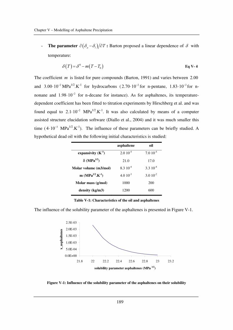
Chapter V – Modelling of Asphaltene Precipitation
189
- The parameter ( )a l Tδ δ∂ − ∂ : Barton proposed a linear dependence of δ with
temperature:
( ) ( )00T m T Tδ δ= − − Eq V- 4
The coefficient m is listed for pure compounds (Barton, 1991) and varies between 2.00
and 23.00 10−⋅ MPa1/2.K-1 for hydrocarbons ( 22.70 10−⋅ for n-pentane, 21.83 10−⋅ for n-
nonane and 21.98 10−⋅ for n-decane for instance). As for asphaltenes, its temperature-
dependent coefficient has been fitted to titration experiments by Hirschberg et al. and was
found equal to 22.1 10−⋅ MPa1/2.K-1. It was also calculated by means of a computer
assisted structure elucidation software (Diallo et al., 2004) and it was much smaller this
time ( 34 10−⋅ MPa1/2.K-1). The influence of these parameters can be briefly studied. A
hypothetical dead oil with the following initial characteristics is studied:
asphaltene oil
expansivity (K-1) 2.0 10-4 7.0 10-4
δ (MPa1/2) 21.0 17.0
Molar volume (m3/mol) 8.3 10-4 3.3 10-4
m (MPa1/2.K-1) 4.0 10-3 3.0 10-2
Molar mass (g/mol) 1000 200
density (kg/m3) 1200 600
Table V-1: Characteristics of the oil and asphaltenes
The influence of the solubility parameter of the asphaltenes is presented in Figure V-1.
0.0E+00
5.0E-04
1.0E-03
1.5E-03
2.0E-03
2.5E-03
21.8 22 22.2 22.4 22.6 22.8 23 23.2
solubility parameter asphaltenes (MPa 1/2)
x_as
ph
alte
nes
Figure V-1: Influence of the solubility parameter of the asphaltenes on their solubility
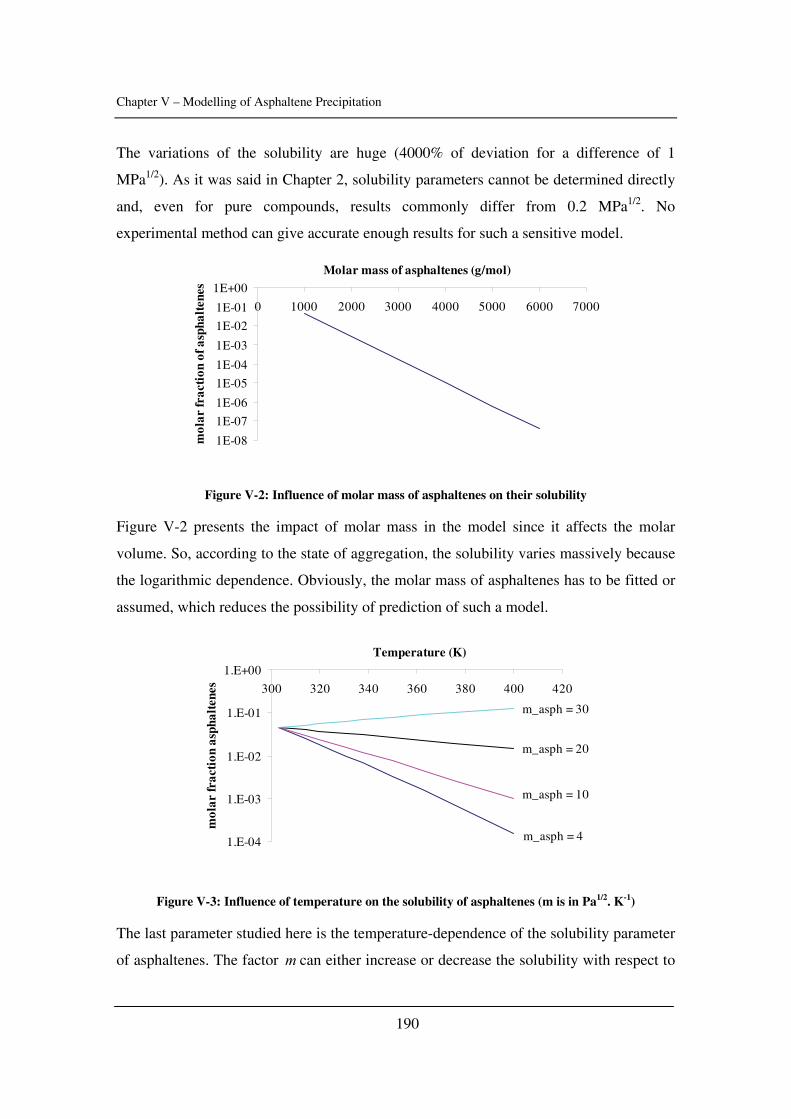
Chapter V – Modelling of Asphaltene Precipitation
190
The variations of the solubility are huge (4000% of deviation for a difference of 1
MPa1/2). As it was said in Chapter 2, solubility parameters cannot be determined directly
and, even for pure compounds, results commonly differ from 0.2 MPa1/2. No
experimental method can give accurate enough results for such a sensitive model.
1E-08
1E-07
1E-06
1E-05
1E-04
1E-03
1E-02
1E-01
1E+00
0 1000 2000 3000 4000 5000 6000 7000
Molar mass of asphaltenes (g/mol)
mol
ar fr
acti
on o
f asp
halt
enes
Figure V-2: Influence of molar mass of asphaltenes on their solubility
Figure V-2 presents the impact of molar mass in the model since it affects the molar
volume. So, according to the state of aggregation, the solubility varies massively because
the logarithmic dependence. Obviously, the molar mass of asphaltenes has to be fitted or
assumed, which reduces the possibility of prediction of such a model.
m_asph = 20
m_asph = 30
m_asph = 4
m_asph = 10
1.E-04
1.E-03
1.E-02
1.E-01
1.E+00
300 320 340 360 380 400 420
Temperature (K)
mol
ar fr
acti
on a
spha
lten
es
Figure V-3: Influence of temperature on the solubility of asphaltenes (m is in Pa1/2. K-1)
The last parameter studied here is the temperature-dependence of the solubility parameter
of asphaltenes. The factor m can either increase or decrease the solubility with respect to
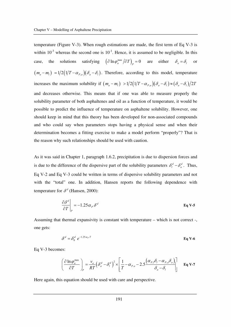
Chapter V – Modelling of Asphaltene Precipitation
191
temperature (Figure V-3). When rough estimations are made, the first term of Eq V-3 is
within 10-3 whereas the second one is 10-1. Hence, it is assumed to be negligible. In this
case, the solutions satisfying ( )maxln 0a PTϕ∂ ∂ = are either a lδ δ= or
( ) ( )( ),1 2 1a l P a a lm m T α δ δ− = − − . Therefore, according to this model, temperature
increases the maximum solubility if ( ) ( )( ) ( ),1 2 1 2a l P a a l a lm m T Tα δ δ δ δ− > − − ≈ −
and decreases otherwise. This means that if one was able to measure properly the
solubility parameter of both asphaltenes and oil as a function of temperature, it would be
possible to predict the influence of temperature on asphaltene solubility. However, one
should keep in mind that this theory has been developed for non-associated compounds
and who could say when parameters stops having a physical sense and when their
determination becomes a fitting exercise to make a model perform “properly”? That is
the reason why such relationships should be used with caution.
As it was said in Chapter 1, paragraph 1.6.2, precipitation is due to dispersion forces and
is due to the difference of the dispersive part of the solubility parameters d dl aδ δ− . Thus,
Eq V-2 and Eq V-3 could be written in terms of dispersive solubility parameters and not
with the “total” one. In addition, Hansen reports the following dependence with
temperature for dδ (Hansen, 2000):
1.25d
dP
PTδ α δ∂
= −∂
Eq V-5
Assuming that thermal expansivity is constant with temperature – which is not correct -,
one gets:
1.250
P Td d e αδ δ −= Eq V-6
Eq V-3 becomes:
( ) ( )max 2 , ,.
ln 1 2.5 P l l P a ad da aa l P a
a lP
vT RT T
α δ α δϕ δ δ αδ δ
⎡ ⎤−⎛ ⎞∂= − × − −⎢ ⎥⎜ ⎟∂ −⎢ ⎥⎝ ⎠ ⎣ ⎦
Eq V-7
Here again, this equation should be used with care and perspective.
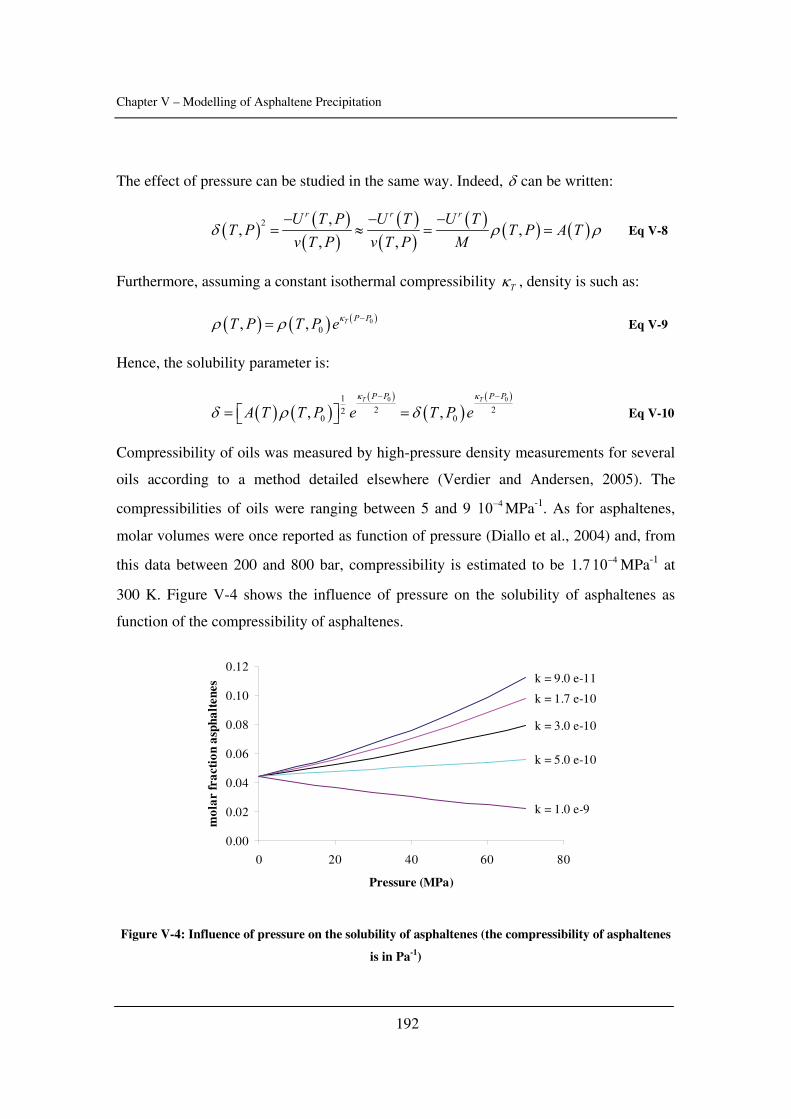
Chapter V – Modelling of Asphaltene Precipitation
192
The effect of pressure can be studied in the same way. Indeed, δ can be written:
( ) ( )( )
( )( )
( ) ( ) ( )2 ,, ,
, ,
r r rU T P U T U TT P T P A T
v T P v T P Mδ ρ ρ
− − −= ≈ = = Eq V-8
Furthermore, assuming a constant isothermal compressibility Tκ , density is such as:
( ) ( ) ( )00, , T P PT P T P eκρ ρ −= Eq V-9
Hence, the solubility parameter is:
( ) ( )( )
( )( )0 01
2 220 0, ,
T TP P P P
A T T P e T P eκ κ
δ ρ δ− −
= =⎡ ⎤⎣ ⎦ Eq V-10
Compressibility of oils was measured by high-pressure density measurements for several
oils according to a method detailed elsewhere (Verdier and Andersen, 2005). The
compressibilities of oils were ranging between 5 and 9 410− MPa-1. As for asphaltenes,
molar volumes were once reported as function of pressure (Diallo et al., 2004) and, from
this data between 200 and 800 bar, compressibility is estimated to be 41.7 10− MPa-1 at
300 K. Figure V-4 shows the influence of pressure on the solubility of asphaltenes as
function of the compressibility of asphaltenes.
k = 9.0 e-11
k = 1.7 e-10
k = 3.0 e-10
k = 5.0 e-10
k = 1.0 e-9
0.00
0.02
0.04
0.06
0.08
0.10
0.12
0 20 40 60 80
Pressure (MPa)
mol
ar fr
acti
on a
spha
lten
es
Figure V-4: Influence of pressure on the solubility of asphaltenes (the compressibility of asphaltenes
is in Pa-1)
Chapter V – Modelling of Asphaltene Precipitation
193
The influence of pressure in much less than temperature on the solubility and the
equation is hence much less dependent on the input factors relevant to pressure, i.e. the
compressibilities. Pressure increases the solubility as it is known experimentally. If the
compressibility of asphaltenes is larger than the one of the solvent, pressure happens to
decreases solubility. This has of course not much physical sense.
Many more calculations could be made with such a model, especially with the effect of
gas on the solubility parameter of the solvent. However, as Andersen and Speight spotted
it, it is necessary to recognize the lack of resemblance between this model and the true
nature of asphaltenes (Andersen and Speight, 1999). Many other groups worked with the
Flory-Huggins theory: for instance, Yarranton’s group from the University of Calgary
combined it with a mass distribution of the asphaltenes and developed correlations of the
different parameters (see Alboudwarej et al., 2005 for instance). The system is
characterized and the equilibrium is solved with the Rachford-Rice equation. The amount
of precipitated asphaltenes can be fitted with good accuracy.
1.2.2. The Scatchard-Hildebrand equation
This approach assumes that the regular solution theory applies to the crude oil (Griffith
and Siegmund, 1985). Assuming that the activity of asphaltenes is unity,
( )22ln a l l aa
RTxv
ϕ δ δ= − − Eq V-11
where ax is the fraction of soluble asphaltenes and lϕ the volume fraction of the liquid
medium.
The same derivations with temperature as in the previous paragraph can be done and the
same conclusions drawn. In addition, this model does not take aggregation into account
since it states that there is no specific interaction.
1.2.3. The Scott-Magat equation
One other important feature of asphaltenes is their molar distribution (chapter 1,
paragraph 1.3). Kawanaka and co-workers applied this distribution by means of the Scott-
Magat equation (Kawanaka et al., 1991). The Flory interaction parameter was modified
Chapter V – Modelling of Asphaltene Precipitation
194
with the introduction of an interaction parameter 12l and with a statistical entropic term
l z . The experimental fit turned out to be good thanks to the additional parameters but
the predictions remained poor. Phase diagrams of mixtures CO2-oils were also
investigated. In total, six parameters were tuned to experimental data in order to fit the
results.
1.2.4. Cubic equations of state
Cubic equations of state were not so much investigated. Gupta coupled a solid phase
fugacity with a Peng-Robinson model (Gupta, 1986). The critical parameters are obtained
from the Alexander’s correlations combining NMR data and the SRK EOS. However, as
seen in Chapter 3, paragraph 3.2.2, the heteroatom content and the choice of the molar
weight are crucial and can give irrelevant results. The interaction parameters ijk were the
key parameters to fit in order to get the proper trends in solubility. However, they had to
be fitted for every n-alkane used during the titrations thought they should be constant
(Andersen and Speight, 1999).
Szewczyk and Béhar desribed the flocculation as the formation of a new liquid phase
with a high asphaltenic content (Szewczyk and Béhar, 1999) (note that they used the
word “flocculation” and not “precipitation” to describe the phase transition and the term
“deposit” instead of “precipitated asphaltenes”). The crude oil is represented by a light
fraction (F11-F20) and the F20+ heavy fraction is divided into four pseudo-components.
The critical properties are estimated by a group contribution method and the PR EOS is
used in combination with specific mixing rules. The critical pressures of the fraction are
fitted to the density at atmospheric conditions and the properties of the asphaltenes are
fitted to the amount of precipitated asphaltenes at 303.15 K. This fitting procedure
enables a proper description of the saturation pressures, the relative volumes and the
flocculation curves.
The Computer Modelling Group (Calgary, Canada) modelled the precipitated asphaltene
as a dense phase, either liquid or solid (Nghiem et al., 1993). The asphaltene fraction is
Chapter V – Modelling of Asphaltene Precipitation
195
divided into two: a precipitating and a non-precipitating component. The PR EOS was
used as well with interaction parameters. However, they do not explain how the critical
parameters were obtained and what their values are. Hence, they might have slightly
more than two or three fitting parameters, as they claim. The interaction parameters were
used to fit the precipitation curve.
To conclude, the cubic EOS are very popular in the calculation of phase equilibria and
especially in the oil industry. However, the determination of the critical parameters and
the characterization of the oil – especially the heavy fraction – prevent this approach from
being anything else but a good fitting exercise of parameters. The absence of specific
interactions also makes this approach not that physical.
1.2.5. The association EOS
Associating EOS like SAFT are the most advanced EOS, the last branch of the tree. It
seemed quite natural to apply these equations to asphaltene precipitation. Many groups
and famous scientists in the world of chemical engineering tried to apply them: Chapman
(Ting et al., 2003), Prausnitz (Wu et al., 1998; Wu et al., 2000), Firoozabadi (Wu et al.,
1998; Wu et al., 2000), Gil-Villegas (Buenrostro-Gonzalez et al., 2004) or Michelsen
(Christensen et al., 2005) to name a few.
The same problems as for the cubic EOS rise: characterization of the oil (the heavy
fraction particularly) and determination of the parameters. Andersen and Speight
summarized it all: “The more realistic the model becomes, the more complex it will be.
The complexity as well gives rise to an increase in unknown parameters which in turn
will have to be estimated or fitted to experimental data”. (Andersen and Speight, 1999).
Though their respective work is impressive as well as the fitting curves obtained,
especially for gas injection and phase envelopes, the use of SAFT raises fundamental
questions. The two main issues are the absence of the dilution effect and the co-
solubilizing effect of resins (Zhou, 2005).
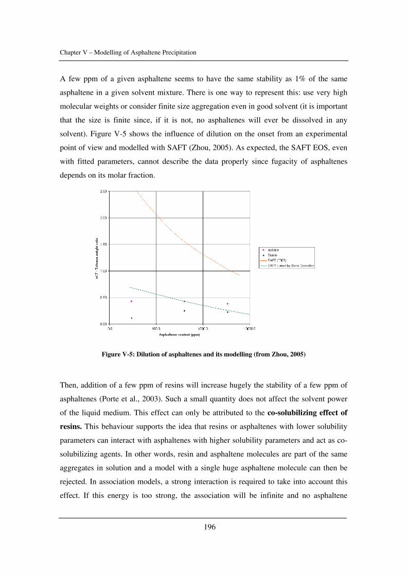
Chapter V – Modelling of Asphaltene Precipitation
196
A few ppm of a given asphaltene seems to have the same stability as 1% of the same
asphaltene in a given solvent mixture. There is one way to represent this: use very high
molecular weights or consider finite size aggregation even in good solvent (it is important
that the size is finite since, if it is not, no asphaltenes will ever be dissolved in any
solvent). Figure V-5 shows the influence of dilution on the onset from an experimental
point of view and modelled with SAFT (Zhou, 2005). As expected, the SAFT EOS, even
with fitted parameters, cannot describe the data properly since fugacity of asphaltenes
depends on its molar fraction.
Figure V-5: Dilution of asphaltenes and its modelling (from Zhou, 2005)
Then, addition of a few ppm of resins will increase hugely the stability of a few ppm of
asphaltenes (Porte et al., 2003). Such a small quantity does not affect the solvent power
of the liquid medium. This effect can only be attributed to the co-solubilizing effect of
resins. This behaviour supports the idea that resins or asphaltenes with lower solubility
parameters can interact with asphaltenes with higher solubility parameters and act as co-
solubilizing agents. In other words, resin and asphaltene molecules are part of the same
aggregates in solution and a model with a single huge asphaltene molecule can then be
rejected. In association models, a strong interaction is required to take into account this
effect. If this energy is too strong, the association will be infinite and no asphaltene
Chapter V – Modelling of Asphaltene Precipitation
197
molecules will be soluble. On the contrary, if the energy is too low, there will be no
association. So, what about choosing an intermediate interaction energy? No energy-
based model can give a centred distribution of the molecules, as it is the case for
asphaltenes. There would be many monomers, a few dimers, a few trimers but less and
so on. Thus, this energy-based model is not sufficient (and SAFT is energy-driven)
(Zhou, 2005).
CPA (Cubic Plus Association, Kontogeorgis et al., 1996) was also used to model
asphaltene precipitation (Knudsen, 2001; Fahim and Andersen, 2005). Fahim and
Andersen found that the error in constructing asphaltene precipitation envelope by SRK
EOS (untuned) has been dropped from 19% to 10% by using the CPA EOS. However,
the final match depends on the initial tuning of SRK. In most cases, the improvement is
within 5%. As Fahim and Andersen said it, “is it technically reasonable?”, i.e. are all
these efforts made to use CPA worth the results for asphaltenic systems?
1.3. Scaling equations
Scaling equations were proposed in 1996, similarly to the ones used in aggregation and
gelation phenomena (Rassamdana et al., 1996). Such a method successfully described the
amount of precipitated asphaltenes as function of the solvent-to-crude oil ratio and the
molar weight of the solvent. A correlation was also proposed for the onset of
precipitation. The same authors wrote several papers, including studies about gas
injection, molecular weight or the structure of the aggregates. Their work about scaling
equations was also further investigated.
1.4. Conclusion
Though thermodynamic models are the solution to model asphaltene precipitation, they
face a dilemma: when they are too complex, the parameters to fit are too numerous and
prevent the modelling from being relevant and when they are too simple, though they can
render some of the properties, they cannot describe all the necessary features. Unless, the
input parameters can be measured or calculated very accurately, all models are bound to
remain fitting exercises.
Chapter V – Modelling of Asphaltene Precipitation
198
2. Asphaltene precipitation and cubic EOS
The approach using cubic EOS seemed fruitful and promising in the few cases it was
used (see paragraph 1.2.4). Obviously, the characterization step is of major importance,
especially the choice of the critical parameters of asphaltenes. Are these parameters
bound to remain fitting parameters or can they be predicted? If yes, what is the required
accuracy? Does a cubic EOS have enough degrees of freedom to describe all the
thermodynamic properties of asphaltenes? This paragraph is a brief attempt to answer
some of these questions.
2.1. The model
In this work, the Peng-Robinson EOS is used. The interactions parameters are set to zero
unless stated otherwise, the same model is used for all the phases, there is no Peneloux
correction for the volume and the Poynting factor is not used neither. Asphaltene
precipitation is treated as liquid-liquid transition. A multiphase flash developed by
Michael Michelsen was used in a Fortran environment. The method to solve the
Rachford-Rice equation as well as the stability analysis is fully described in Michelsen’s
monograph (Michelsen and Møllerup, 2004). The same calculations can be made with the
in-house software SPECS if asphaltenes are entered as a new compound with its
respective parameters. Note that the asphaltene phase is not a pure phase.
2.2. The dilution effect
As Porte et al. (2003) reported it, one of the few known facts about asphaltenes is that
dilution of asphaltene solutions (i.e. asphaltenes in toluene) does not affect the onset. In
order to model such behaviour, it would require that fugacity does not depend on molar
fraction, which is not the case for a cubic EOS.
The system studied here is composed of n-heptane, toluene and asphaltenes (seen as a
pseudo-component). Table V-2 gives the respective critical parameters. The working
conditions are 300 K and 0.1 MPa. For the conversion in ppm (mg/L), the density of
toluene and n-heptane were calculated with the DIPPR correlations. Density of
asphaltenes was assumed to be 1200 kg/m3 and with a molar mass of 1000 g/mol.
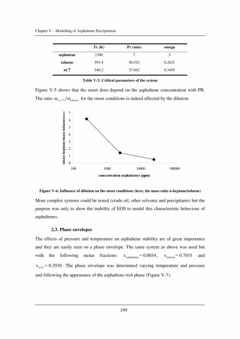
Chapter V – Modelling of Asphaltene Precipitation
199
Tc (K) Pc (atm) omega
asphatene 1300 7 3
toluene 591.8 40.523 0.2621
nC7 540.2 27.042 0.3495
Table V-2: Critical parameters of the system
Figure V-5 shows that the onset does depend on the asphaltene concentration with PR.
The ratio 7n C toluenem m− for the onset conditions is indeed affected by the dilution.
0
1
2
3
4
5
6
7
100 1000 10000 100000
concentration asphaltenes (ppm)
(mas
s hep
tane
/mas
s tol
uene
) ons
et
Figure V-6: Influence of dilution on the onset conditions (here, the mass ratio n-heptane/toluene)
More complex systems could be tested (crude oil, other solvents and precipitants) but the
purpose was only to show the inability of EOS to model this characteristic behaviour of
asphaltenes.
2.3. Phase envelopes
The effects of pressure and temperature on asphaltene stability are of great importance
and they are easily seen on a phase envelope. The same system as above was used but
with the following molar fractions: asphaltenesx = 0.0034 , toluenex = 0.7035 and
n-C7x = 0.2930 . The phase envelope was determined varying temperature and pressure
and following the appearance of the asphaltene-rich phase (Figure V-7).
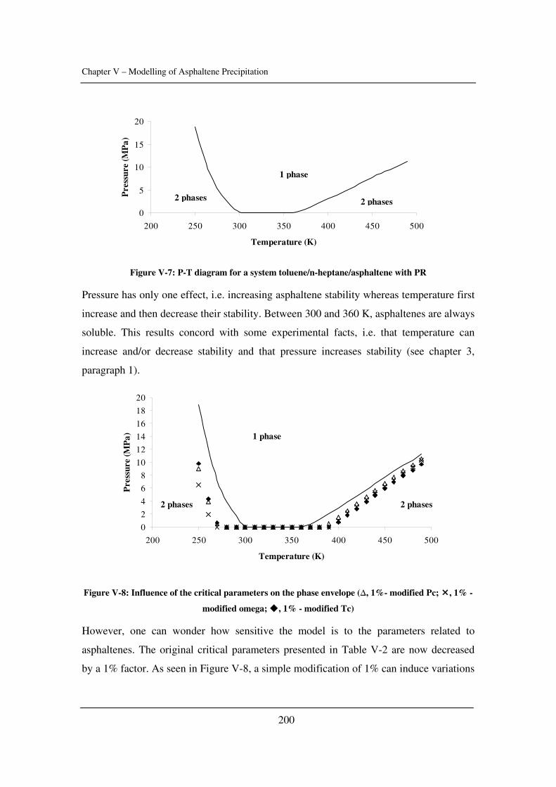
Chapter V – Modelling of Asphaltene Precipitation
200
0
5
10
15
20
200 250 300 350 400 450 500
Temperature (K)
Pre
ssur
e (M
Pa)
2 phases2 phases
1 phase
Figure V-7: P-T diagram for a system toluene/n-heptane/asphaltene with PR
Pressure has only one effect, i.e. increasing asphaltene stability whereas temperature first
increase and then decrease their stability. Between 300 and 360 K, asphaltenes are always
soluble. This results concord with some experimental facts, i.e. that temperature can
increase and/or decrease stability and that pressure increases stability (see chapter 3,
paragraph 1).
0
2
4
6
8
10
12
14
16
18
20
200 250 300 350 400 450 500
Temperature (K)
Pre
ssur
e (M
Pa) 1 phase
2 phases 2 phases
Figure V-8: Influence of the critical parameters on the phase envelope (∆, 1%- modified Pc; , 1% -
modified omega; , 1% - modified Tc)
However, one can wonder how sensitive the model is to the parameters related to
asphaltenes. The original critical parameters presented in Table V-2 are now decreased
by a 1% factor. As seen in Figure V-8, a simple modification of 1% can induce variations
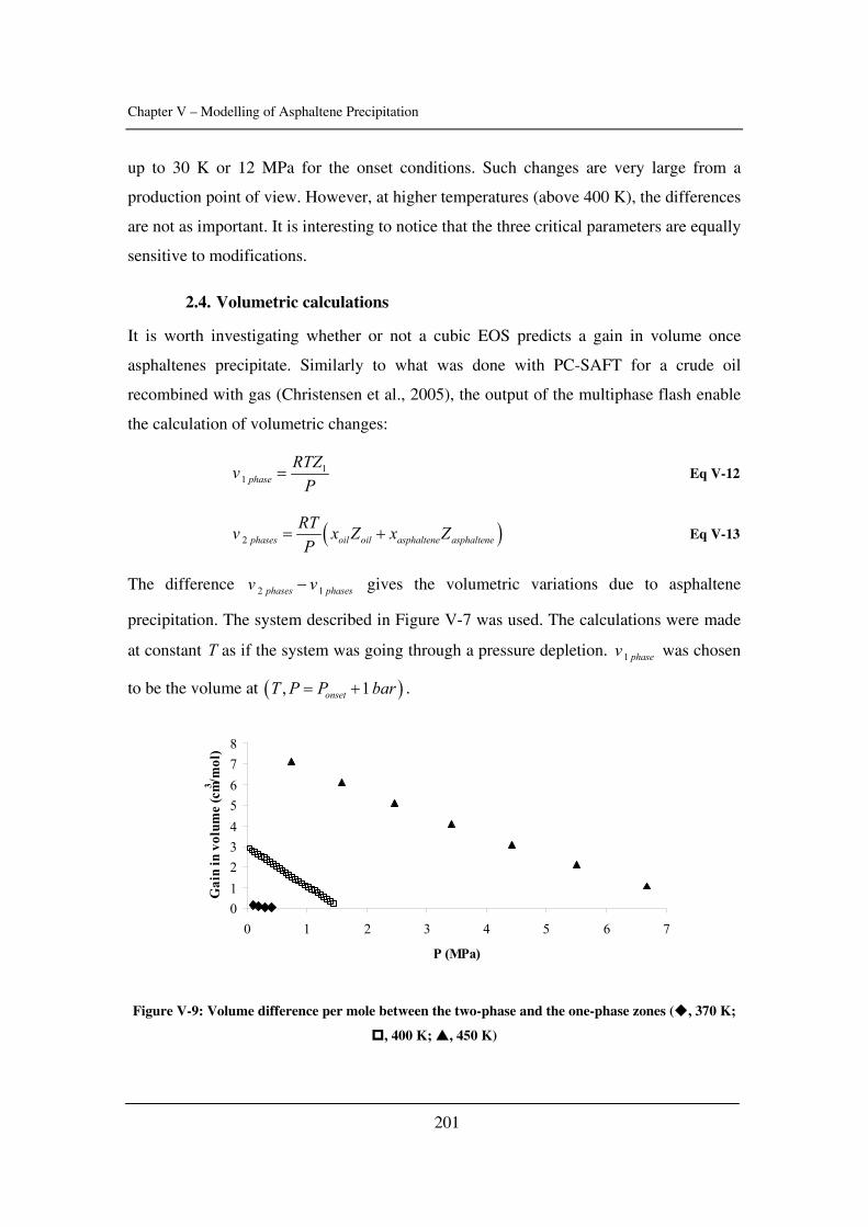
Chapter V – Modelling of Asphaltene Precipitation
201
up to 30 K or 12 MPa for the onset conditions. Such changes are very large from a
production point of view. However, at higher temperatures (above 400 K), the differences
are not as important. It is interesting to notice that the three critical parameters are equally
sensitive to modifications.
2.4. Volumetric calculations
It is worth investigating whether or not a cubic EOS predicts a gain in volume once
asphaltenes precipitate. Similarly to what was done with PC-SAFT for a crude oil
recombined with gas (Christensen et al., 2005), the output of the multiphase flash enable
the calculation of volumetric changes:
11 phase
RTZvP
= Eq V-12
( )2 phases oil oil asphaltene asphalteneRTv x Z x ZP
= + Eq V-13
The difference 2 1phases phasesv v− gives the volumetric variations due to asphaltene
precipitation. The system described in Figure V-7 was used. The calculations were made
at constant T as if the system was going through a pressure depletion. 1 phasev was chosen
to be the volume at ( ), 1onsetT P P bar= + .
012345678
0 1 2 3 4 5 6 7
P (MPa)
Gai
n in
vol
ume
(cm3 /m
ol)
Figure V-9: Volume difference per mole between the two-phase and the one-phase zones ( , 370 K;
, 400 K; , 450 K)
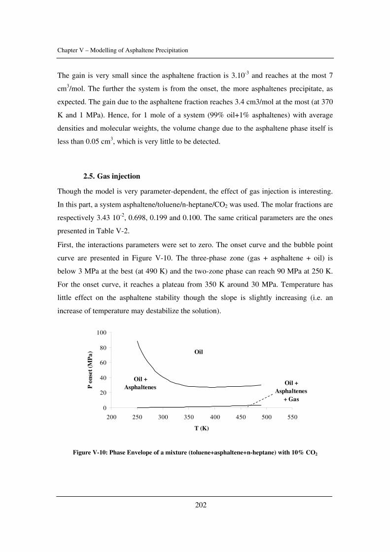
Chapter V – Modelling of Asphaltene Precipitation
202
The gain is very small since the asphaltene fraction is 3.10-3 and reaches at the most 7
cm3/mol. The further the system is from the onset, the more asphaltenes precipitate, as
expected. The gain due to the asphaltene fraction reaches 3.4 cm3/mol at the most (at 370
K and 1 MPa). Hence, for 1 mole of a system (99% oil+1% asphaltenes) with average
densities and molecular weights, the volume change due to the asphaltene phase itself is
less than 0.05 cm3, which is very little to be detected.
2.5. Gas injection
Though the model is very parameter-dependent, the effect of gas injection is interesting.
In this part, a system asphaltene/toluene/n-heptane/CO2 was used. The molar fractions are
respectively 3.43 10-2, 0.698, 0.199 and 0.100. The same critical parameters are the ones
presented in Table V-2.
First, the interactions parameters were set to zero. The onset curve and the bubble point
curve are presented in Figure V-10. The three-phase zone (gas + asphaltene + oil) is
below 3 MPa at the best (at 490 K) and the two-zone phase can reach 90 MPa at 250 K.
For the onset curve, it reaches a plateau from 350 K around 30 MPa. Temperature has
little effect on the asphaltene stability though the slope is slightly increasing (i.e. an
increase of temperature may destabilize the solution).
0
20
40
60
80
100
200 250 300 350 400 450 500 550
T (K)
P o
nset
(MP
a) Oil
Oil + Asphaltenes
Oil + Asphaltenes
+ Gas
Figure V-10: Phase Envelope of a mixture (toluene+asphaltene+n-heptane) with 10% CO2
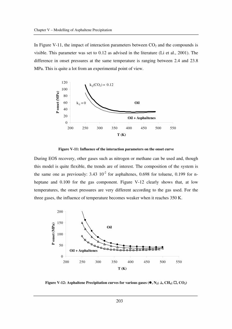
Chapter V – Modelling of Asphaltene Precipitation
203
In Figure V-11, the impact of interaction parameters between CO2 and the compounds is
visible. This parameter was set to 0.12 as advised in the literature (Li et al., 2001). The
difference in onset pressures at the same temperature is ranging between 2.4 and 23.8
MPa. This is quite a lot from an experimental point of view.
0
20
40
60
80
100
120
200 250 300 350 400 450 500 550
T (K)
P o
nset
(MP
a)
Oil
Oil + Asphaltenes
kij(CO2) = 0.12
kij = 0
Figure V-11: Influence of the interaction parameters on the onset curve
During EOS recovery, other gases such as nitrogen or methane can be used and, though
this model is quite flexible, the trends are of interest. The composition of the system is
the same one as previously: 3.43 10-2 for asphaltenes, 0.698 for toluene, 0.199 for n-
heptane and 0.100 for the gas component. Figure V-12 clearly shows that, at low
temperatures, the onset pressures are very different according to the gas used. For the
three gases, the influence of temperature becomes weaker when it reaches 350 K.
0
50
100
150
200
200 250 300 350 400 450 500 550
T (K)
P o
nset
(MP
a)
Oil
Oil + Asphaltenes
Figure V-12: Asphaltene Precipitation curves for various gases ( , N2; ∆, CH4; , CO2)
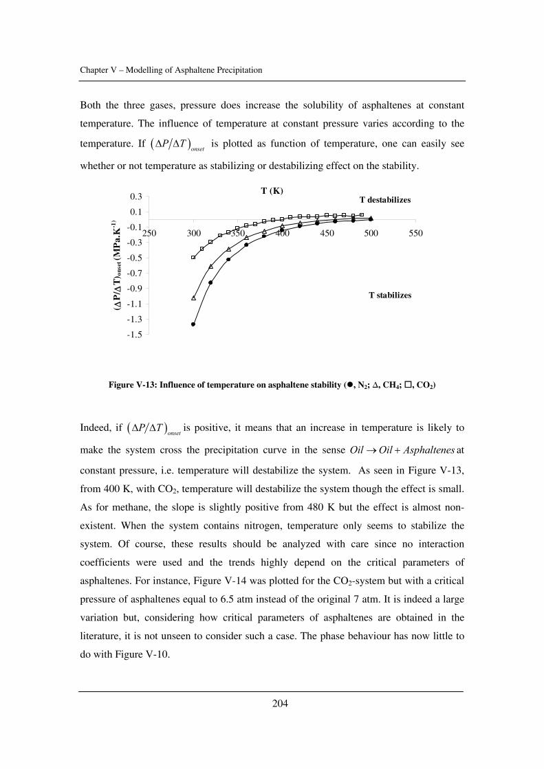
Chapter V – Modelling of Asphaltene Precipitation
204
Both the three gases, pressure does increase the solubility of asphaltenes at constant
temperature. The influence of temperature at constant pressure varies according to the
temperature. If ( )onsetP TΔ Δ is plotted as function of temperature, one can easily see
whether or not temperature as stabilizing or destabilizing effect on the stability.
-1.5
-1.3
-1.1
-0.9
-0.7
-0.5
-0.3
-0.1
0.1
0.3
250 300 350 400 450 500 550
T (K)
( ΔP
/ ΔT
) ons
et (M
Pa.
K-1
)
T destabilizes
T stabilizes
Figure V-13: Influence of temperature on asphaltene stability ( , N2; ∆, CH4; , CO2)
Indeed, if ( )onsetP TΔ Δ is positive, it means that an increase in temperature is likely to
make the system cross the precipitation curve in the sense Oil Oil Asphaltenes→ + at
constant pressure, i.e. temperature will destabilize the system. As seen in Figure V-13,
from 400 K, with CO2, temperature will destabilize the system though the effect is small.
As for methane, the slope is slightly positive from 480 K but the effect is almost non-
existent. When the system contains nitrogen, temperature only seems to stabilize the
system. Of course, these results should be analyzed with care since no interaction
coefficients were used and the trends highly depend on the critical parameters of
asphaltenes. For instance, Figure V-14 was plotted for the CO2-system but with a critical
pressure of asphaltenes equal to 6.5 atm instead of the original 7 atm. It is indeed a large
variation but, considering how critical parameters of asphaltenes are obtained in the
literature, it is not unseen to consider such a case. The phase behaviour has now little to
do with Figure V-10.
Chapter V – Modelling of Asphaltene Precipitation
205
0
5
10
15
20
25
200 250 300 350 400 450 500 550
T (K)
P (M
Pa)
Oil Oil + Asphaltenes
Oil + Asphaltenes+ Gas
Figure V-14: Influence of Pc(asphaltene) on the phase envelope in presence of CO2
So, what are the conclusions of such modelling?
- The cubic EOS can not render the absence of dilution effect.
- Obviously, any phase envelope can be described considering the dependence to
the critical parameters of asphaltenes.
- The model can detect asphaltene precipitation due to gas injection
- The interaction coefficients can be used as additional fitting parameters
- Pressure increases asphaltene stability whereas temperature can both destabilize
and stabilize asphaltenic fluids.
Much more could be done with this model but the objective was not to evaluate the
model but rather to show how sensitive and flexible it is when dealing with asphaltenes.
Chapter V – Modelling of Asphaltene Precipitation
206
3. A new approach combining aggregation and cubic EOS
The idea is to establish a model able to describe and predict asphaltene precipitation,
taking into account the association of asphaltene molecules into nano-aggregates (Zhou et
al., 2005). The precipitation occurs when the asphaltene phase is in equilibrium with the
bulk phase (the crude oil).
In spite of an often complex scheme and a large number of fitting parameters, most of
models invoking association do not allow representation of the simple fact that the
asphaltene nano-aggregates in terms of size are insensitive to dilution in good solvents or
a change in solvent quality when the solution is far from the precipitation threshold. The
description of the mechanism of nano-aggregation by these models depends on the
balance between the energy of association in opposition to the dispersive term. Thus, in
some cases, the aggregates tend to grow indefinitely or, in other cases, to disappear
completely. The geometry of the nano-aggregates is very difficult to take into account by
these models.
Regarding this difficulty, a description proposed lately seems to be an attractive
alternative (Porte et al., 2003). This description is based on a simple idea: on one side, the
forces involved in the colloidal aggregation and on the other side, those driving the
precipitation are different in nature and strength. The aggregation is driven by strong
specific forces and the size of the aggregates is limited for geometric reason; therefore the
aggregates are insensitive to the quality of the apolar solvent. The precipitation is
determined by the weaker and non-specific dispersion forces. Using this picture, any
equation of state can be modified for the description of asphaltene dissolution –
precipitation.
3.1. The TOTAL model
The assumptions are as follows:
- Asphaltene molecules are associated into aggregates having an equal number of
asphaltene molecules. This number, noted N , is called the aggregation number
- There can be several types of asphaltenes but every molecule has the same
number of “binding sites” SN
Chapter V – Modelling of Asphaltene Precipitation
207
- The association energy per bonding is equal for any asphaltene molecule
- The number of free asphaltene molecules is very small regarding the number of
associated asphaltene molecules.
Let us consider the following reaction:
iN molecules aggregate⋅ ⇔∑
Therefore, one can write the relation between the concentration of associated molecules
of asphaltenes and free molecule. The first case-scenario is the mono-dispersed
asphaltene. In this case, the chemical reaction is:
N molecules aggregate⇔
The thermodynamic equilibrium of a chemical reaction is described by:
0 ln 0rG RT KΔ + = Eq V-14
where 0 , ,o aggr o freerG Nμ μΔ = − is the standard reaction Gibbs energy and K the
equilibrium constant.
This constant can be written as follows:
ii
i
K a ν=∏ Eq V-15
where ia is the activity coefficient and iν is the stoichiometric coefficient (positive
integer for products, negative integer for reactants).
Thus, taking into account the chemical reaction mentioned above, the thermodynamic
equilibrium is such as:
( )0 ln 0
aggagga a
r Nfree freea a
xG RTx
γ
γ
⎡ ⎤⎢ ⎥Δ + =⎢ ⎥⎣ ⎦
Eq V-16
( ) ( )0 ln ln 0
agg agg
free free
a ar N N
a a
xG RT RTx
γ
γ
⎡ ⎤ ⎡ ⎤⎢ ⎥ ⎢ ⎥Δ + + =⎢ ⎥ ⎢ ⎥⎢ ⎥ ⎢ ⎥⎣ ⎦ ⎣ ⎦
Eq V-17
The superscript agg and free refers respectively to the aggregated and free asphaltenes.
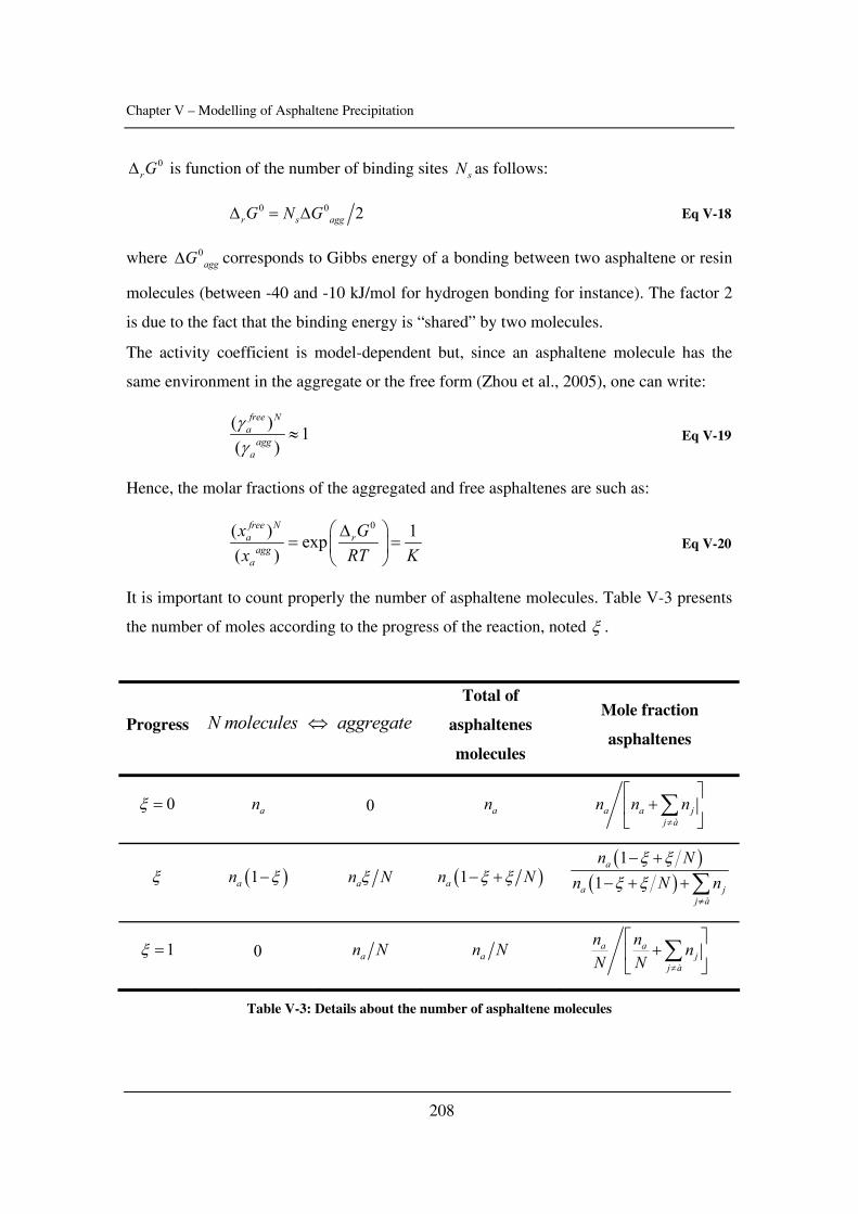
Chapter V – Modelling of Asphaltene Precipitation
208
0rGΔ is function of the number of binding sites sN as follows:
0 0 2r s aggG N GΔ = Δ Eq V-18
where 0aggGΔ corresponds to Gibbs energy of a bonding between two asphaltene or resin
molecules (between -40 and -10 kJ/mol for hydrogen bonding for instance). The factor 2
is due to the fact that the binding energy is “shared” by two molecules.
The activity coefficient is model-dependent but, since an asphaltene molecule has the
same environment in the aggregate or the free form (Zhou et al., 2005), one can write:
( ) 1( )
free Na
agga
γγ
≈ Eq V-19
Hence, the molar fractions of the aggregated and free asphaltenes are such as:
0( ) 1exp( )
free Na r
agga
x Gx RT K
⎛ ⎞Δ= =⎜ ⎟
⎝ ⎠ Eq V-20
It is important to count properly the number of asphaltene molecules. Table V-3 presents
the number of moles according to the progress of the reaction, noted ξ .
Progress N molecules aggregate⇔
Total of
asphaltenes
molecules
Mole fraction
asphaltenes
0ξ = an 0 an a a jj à
n n n≠
⎡ ⎤+⎢ ⎥
⎣ ⎦∑
ξ ( )1an ξ− an Nξ ( )1an Nξ ξ− + ( )
( )1
1a
a jj à
n Nn N n
ξ ξξ ξ
≠
− +− + +∑
1ξ = 0 an N an N a aj
j à
n n nN N ≠
⎡ ⎤+⎢ ⎥
⎣ ⎦∑
Table V-3: Details about the number of asphaltene molecules
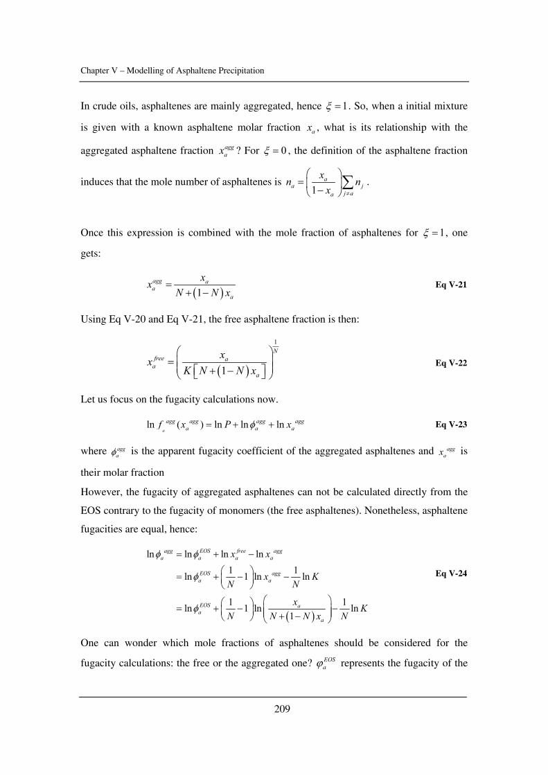
Chapter V – Modelling of Asphaltene Precipitation
209
In crude oils, asphaltenes are mainly aggregated, hence 1ξ = . So, when a initial mixture
is given with a known asphaltene molar fraction ax , what is its relationship with the
aggregated asphaltene fraction aggax ? For 0ξ = , the definition of the asphaltene fraction
induces that the mole number of asphaltenes is 1
aa j
j aa
xn nx ≠
⎛ ⎞= ⎜ ⎟−⎝ ⎠
∑ .
Once this expression is combined with the mole fraction of asphaltenes for 1ξ = , one
gets:
( )1agg aa
a
xxN N x
=+ −
Eq V-21
Using Eq V-20 and Eq V-21, the free asphaltene fraction is then:
( )
1
1
Nfree a
aa
xxK N N x
⎛ ⎞= ⎜ ⎟⎜ ⎟+ −⎡ ⎤⎣ ⎦⎝ ⎠
Eq V-22
Let us focus on the fugacity calculations now.
ln ( ) ln ln lna
agg agg agg agga a af x P xφ= + + Eq V-23
where aggaφ is the apparent fugacity coefficient of the aggregated asphaltenes and agg
ax is
their molar fraction
However, the fugacity of aggregated asphaltenes can not be calculated directly from the
EOS contrary to the fugacity of monomers (the free asphaltenes). Nonetheless, asphaltene
fugacities are equal, hence:
( )
ln ln ln ln1 1ln 1 ln ln
1 1ln 1 ln ln1
agg EOS free agga a a a
EOS agga a
EOS aa
a
x x
x KN N
x KN N N x N
φ φ
φ
φ
= + −
⎛ ⎞= + − −⎜ ⎟⎝ ⎠
⎛ ⎞⎛ ⎞= + − −⎜ ⎟⎜ ⎟ ⎜ ⎟+ −⎝ ⎠ ⎝ ⎠
Eq V-24
One can wonder which mole fractions of asphaltenes should be considered for the
fugacity calculations: the free or the aggregated one? EOSaϕ represents the fugacity of the
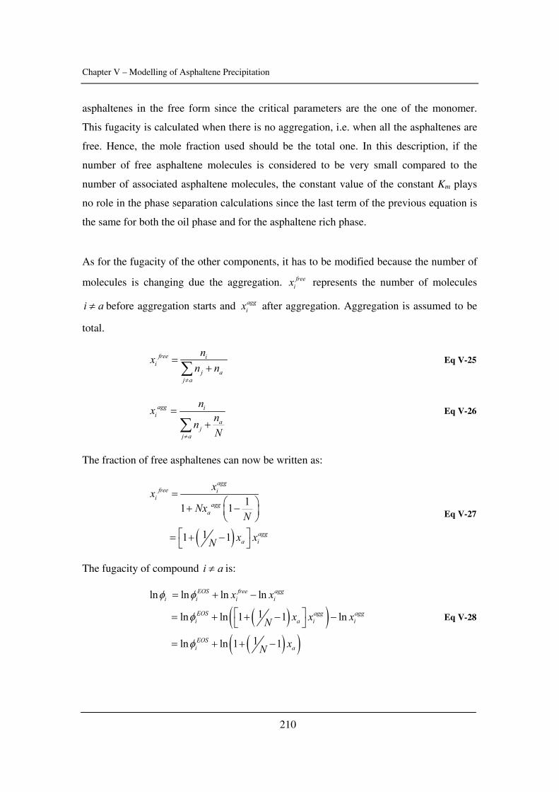
Chapter V – Modelling of Asphaltene Precipitation
210
asphaltenes in the free form since the critical parameters are the one of the monomer.
This fugacity is calculated when there is no aggregation, i.e. when all the asphaltenes are
free. Hence, the mole fraction used should be the total one. In this description, if the
number of free asphaltene molecules is considered to be very small compared to the
number of associated asphaltene molecules, the constant value of the constant Km plays
no role in the phase separation calculations since the last term of the previous equation is
the same for both the oil phase and for the asphaltene rich phase.
As for the fugacity of the other components, it has to be modified because the number of
molecules is changing due the aggregation. freeix represents the number of molecules
i a≠ before aggregation starts and aggix after aggregation. Aggregation is assumed to be
total.
free ii
j aj a
nxn n
≠
=+∑
Eq V-25
agg ii
aj
j a
nx nnN≠
=+∑
Eq V-26
The fraction of free asphaltenes can now be written as:
( )
11 1
11 1
aggfree i
iagg
a
agga i
xxNx
N
x xN
=⎛ ⎞+ −⎜ ⎟⎝ ⎠
⎡ ⎤= + −⎣ ⎦
Eq V-27
The fugacity of compound i a≠ is:
( )( )( )( )
ln ln ln ln
1ln ln 1 1 ln
1ln ln 1 1
EOS free aggi i i i
EOS agg aggi a i i
EOSi a
x x
x x xN
xN
φ φ
φ
φ
= + −
⎡ ⎤= + + − −⎣ ⎦
= + + −
Eq V-28
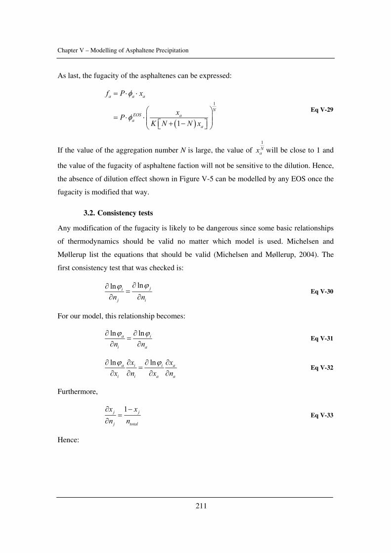
Chapter V – Modelling of Asphaltene Precipitation
211
As last, the fugacity of the asphaltenes can be expressed:
( )
1
1
a a a
NEOS aa
a
f P x
xPK N N x
φ
φ
= ⋅ ⋅
⎛ ⎞= ⋅ ⋅⎜ ⎟⎜ ⎟+ −⎡ ⎤⎣ ⎦⎝ ⎠
Eq V-29
If the value of the aggregation number N is large, the value of Nax1
will be close to 1 and
the value of the fugacity of asphaltene faction will not be sensitive to the dilution. Hence,
the absence of dilution effect shown in Figure V-5 can be modelled by any EOS once the
fugacity is modified that way.
3.2. Consistency tests
Any modification of the fugacity is likely to be dangerous since some basic relationships
of thermodynamics should be valid no matter which model is used. Michelsen and
Møllerup list the equations that should be valid (Michelsen and Møllerup, 2004). The
first consistency test that was checked is:
lnln ji
j in nϕϕ ∂∂
=∂ ∂
Eq V-30
For our model, this relationship becomes:
ln lna i
i an nϕ ϕ∂ ∂
=∂ ∂
Eq V-31
ln lna i i a
i i a a
x xx n x nϕ ϕ∂ ∂ ∂ ∂
=∂ ∂ ∂ ∂
Eq V-32
Furthermore,
1j j
j total
x xn n∂ −
=∂
Eq V-33
Hence:
Chapter V – Modelling of Asphaltene Precipitation
212
ln 1 ln 11 1 1 111 1 1
EOS EOSa i i a
i i total a totala
x xN Nx x n x nx N
ϕ ϕ⎛ ⎞⎛ ⎞∂ − ∂ −− −⎜ ⎟− = −⎜ ⎟ ⎜ ⎟∂ − ∂ ⎡ ⎤⎜ ⎟+ −⎝ ⎠ ⎣ ⎦⎝ ⎠
Eq V-34
Since lnln EOSEOS
ji
j in nϕϕ ∂∂
=∂ ∂
, the previous equation is :
1 11 1 1 111 1 1
i a
i total totala
x xN Nx n nx N
⎛ ⎞⎛ ⎞ − −− −⎜ ⎟=⎜ ⎟ ⎜ ⎟− ⎡ ⎤⎜ ⎟+ −⎝ ⎠ ⎣ ⎦⎝ ⎠
Eq V-35
1111 1
a
a
xx N
⎛ ⎞−⎜ ⎟=⎜ ⎟⎡ ⎤⎜ ⎟+ −⎣ ⎦⎝ ⎠
Eq V-36
1 0N= Eq V-37
N = ∞ Eq V-38
The second consistency test is the Gibbs-Duhem equation:
ln 0ii
i j
nnϕ∂
=∂∑ Eq V-39
For our model, it can be written as :
ln ln 0a ia i
i aa a
n nn nϕ ϕ
≠
∂ ∂+ =
∂ ∂∑ Eq V-40
( )
ln 1 1
ln 1 1 01 1 1
EOSa a
aa a a
EOSi a
ii a a a
xNnx x n
xNnx x N n
ϕ
ϕ
⎛ ⎞∂ ∂−+ +⎜ ⎟∂ ∂⎝ ⎠
⎛ ⎞∂ ∂−− =⎜ ⎟⎜ ⎟∂ + − ∂⎝ ⎠
∑ Eq V-41
( ) ( )1 1 1 1 01 1 1a t a
a a
N Nn n nx x N
⎛ ⎞⎛ ⎞− −+ − − =⎜ ⎟⎜ ⎟ ⎜ ⎟+ −⎝ ⎠ ⎝ ⎠
Eq V-42
( ) ( ) ( )1 11 1 01 1 1t t a
a
Nn N n nx N
⎛ ⎞−− − − =⎜ ⎟⎜ ⎟+ −⎝ ⎠
Eq V-43
Chapter V – Modelling of Asphaltene Precipitation
213
( ) ( ) ( )1 11 1 01 1 1t t a
a
Nn N n nx N
⎛ ⎞−− − − =⎜ ⎟⎜ ⎟+ −⎝ ⎠
Eq V-44
( ) ( )1 1 0
1 1 1t a
ta
n nN nx N
⎡ ⎤−− − =⎢ ⎥+ −⎣ ⎦
Eq V-45
The two solutions are 1N = and N = ∞ .
After checking only two of the consistency tests advised, unrealistic conditions were
found. Hence, though this model is tempting and would solve some if the issues, it does
not seem very wise to use it. However, the approach taking into account aggregation can
be used with no modifications of the fugacity.
3.3. A second approach: the aggregation model
If one makes the same assumptions as for the previous approach, the mole fractions are
modified due to the change of mole numbers. What if the system was considered to be
composed of asphaltene aggregates and i compounds with the following molar fractions:
( )1agg aa
a
xxN N x
=+ −
and ( )1
freeagg ii
a
NxxN N x
=+ −
? What about the thermodynamic model?
The properties of the asphaltenes are the ones of the monomer. Hence, modifications
should be done at one point. As Heidemann and Prausnitz advised it, the a and b
factors can be modified in order to take into account association (Heidemann and
Prausnitz, 1976). They proposed the following mixing rules:
jb jb= Eq V-46
2ja j a= Eq V-47
where the subscript j refers to the aggregate containing j molecules of the monomer.
Once the mole fractions are calculated as well the properties of the pure compounds, a
regular multiphase flash can be used with no further modifications of the fugacities.
Thus, the thermodynamic model would be consistent and aggregation would be taken
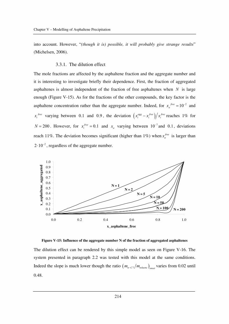
Chapter V – Modelling of Asphaltene Precipitation
214
into account. However, “(though it is) possible, it will probably give strange results”
(Michelsen, 2006).
3.3.1. The dilution effect
The mole fractions are affected by the asphaltene fraction and the aggregate number and
it is interesting to investigate briefly their dependence. First, the fraction of aggregated
asphaltenes is almost independent of the fraction of free asphaltenes when N is large
enough (Figure V-15). As for the fractions of the other compounds, the key factor is the
asphaltene concentration rather than the aggregate number. Indeed, for 210freeax −= and
freeix varying between 0.1 and 0.9 , the deviation ( )agg free free
i i ix x x− reaches 1% for
200N = . However, for 0.1freeix = and ax varying between 710− and 0.1 , deviations
reach 11%. The deviation becomes significant (higher than 1%) when freeax is larger than
22 10−⋅ , regardless of the aggregate number.
0.0
0.10.2
0.3
0.40.5
0.6
0.7
0.80.9
1.0
0.0 0.2 0.4 0.6 0.8 1.0
x_asphaltene_free
x_as
phal
tene
_agg
rega
ted
N = 1
N = 200N = 100
N = 50
N = 10N = 5
N = 2
Figure V-15: Influence of the aggregate number N of the fraction of aggregated asphaltenes
The dilution effect can be rendered by this simple model as seen on Figure V-16. The
system presented in paragraph 2.2 was tested with this model at the same conditions.
Indeed the slope is much lower though the ratio ( )7n C toluene onsetm m− varies from 0.02 until
0.48.
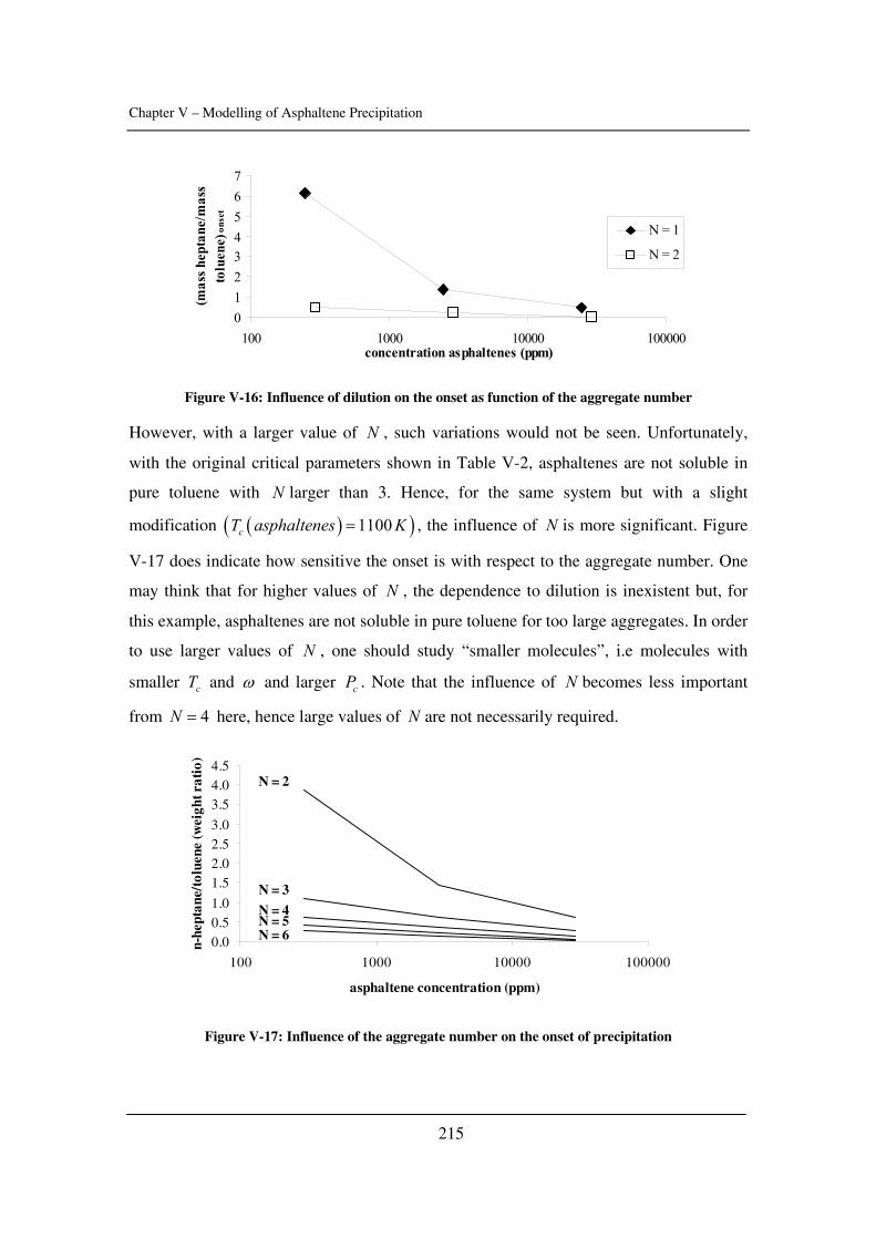
Chapter V – Modelling of Asphaltene Precipitation
215
01234567
100 1000 10000 100000concentration asphaltenes (ppm)
(mas
s hep
tane
/mas
s to
luen
e) on
set
N = 1
N = 2
Figure V-16: Influence of dilution on the onset as function of the aggregate number
However, with a larger value of N , such variations would not be seen. Unfortunately,
with the original critical parameters shown in Table V-2, asphaltenes are not soluble in
pure toluene with N larger than 3. Hence, for the same system but with a slight
modification ( )( )1100cT asphaltenes K= , the influence of N is more significant. Figure
V-17 does indicate how sensitive the onset is with respect to the aggregate number. One
may think that for higher values of N , the dependence to dilution is inexistent but, for
this example, asphaltenes are not soluble in pure toluene for too large aggregates. In order
to use larger values of N , one should study “smaller molecules”, i.e molecules with
smaller cT and ω and larger cP . Note that the influence of N becomes less important
from 4N = here, hence large values of N are not necessarily required.
0.00.51.0
1.52.02.53.0
3.54.04.5
100 1000 10000 100000
asphaltene concentration (ppm)
n-he
ptan
e/to
luen
e (w
eigh
t rat
io)
N = 2
N = 3
N = 4N = 5N = 6
Figure V-17: Influence of the aggregate number on the onset of precipitation
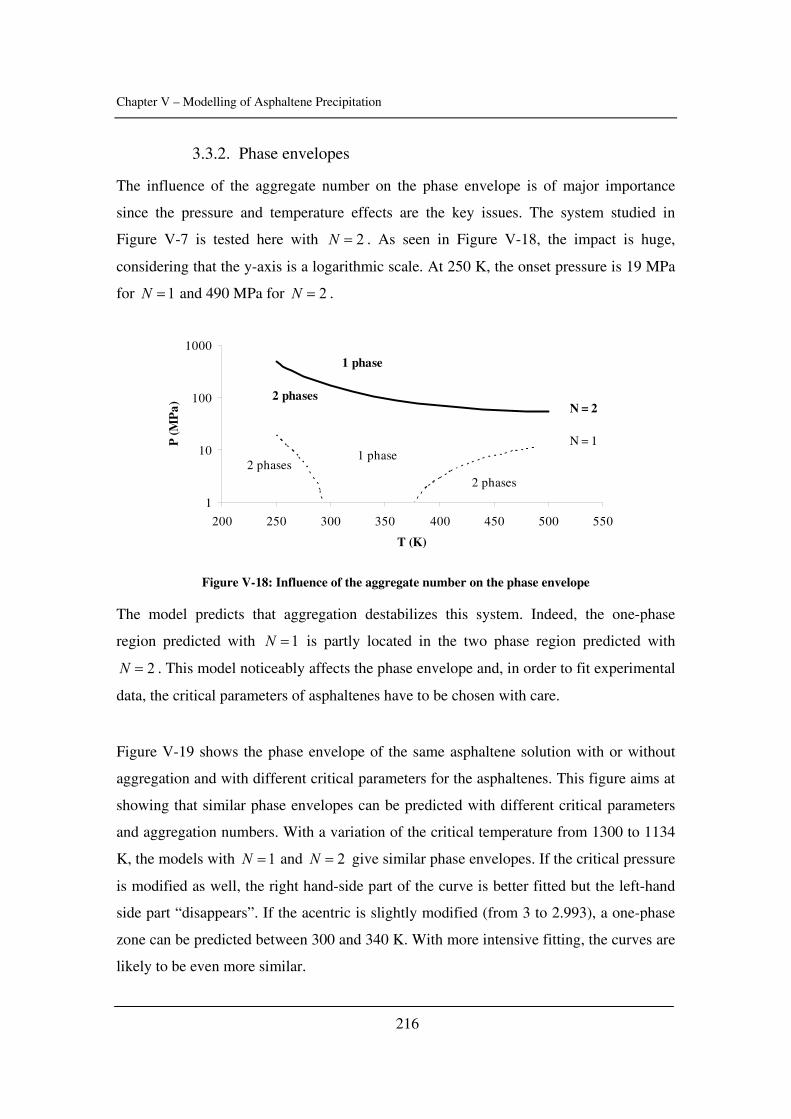
Chapter V – Modelling of Asphaltene Precipitation
216
3.3.2. Phase envelopes
The influence of the aggregate number on the phase envelope is of major importance
since the pressure and temperature effects are the key issues. The system studied in
Figure V-7 is tested here with 2N = . As seen in Figure V-18, the impact is huge,
considering that the y-axis is a logarithmic scale. At 250 K, the onset pressure is 19 MPa
for 1N = and 490 MPa for 2N = .
1
10
100
1000
200 250 300 350 400 450 500 550
T (K)
P (M
Pa)
2 phases2 phases
1 phase
2 phases
1 phase
N = 2
N = 1
Figure V-18: Influence of the aggregate number on the phase envelope
The model predicts that aggregation destabilizes this system. Indeed, the one-phase
region predicted with 1N = is partly located in the two phase region predicted with
2N = . This model noticeably affects the phase envelope and, in order to fit experimental
data, the critical parameters of asphaltenes have to be chosen with care.
Figure V-19 shows the phase envelope of the same asphaltene solution with or without
aggregation and with different critical parameters for the asphaltenes. This figure aims at
showing that similar phase envelopes can be predicted with different critical parameters
and aggregation numbers. With a variation of the critical temperature from 1300 to 1134
K, the models with 1N = and 2N = give similar phase envelopes. If the critical pressure
is modified as well, the right hand-side part of the curve is better fitted but the left-hand
side part “disappears”. If the acentric is slightly modified (from 3 to 2.993), a one-phase
zone can be predicted between 300 and 340 K. With more intensive fitting, the curves are
likely to be even more similar.
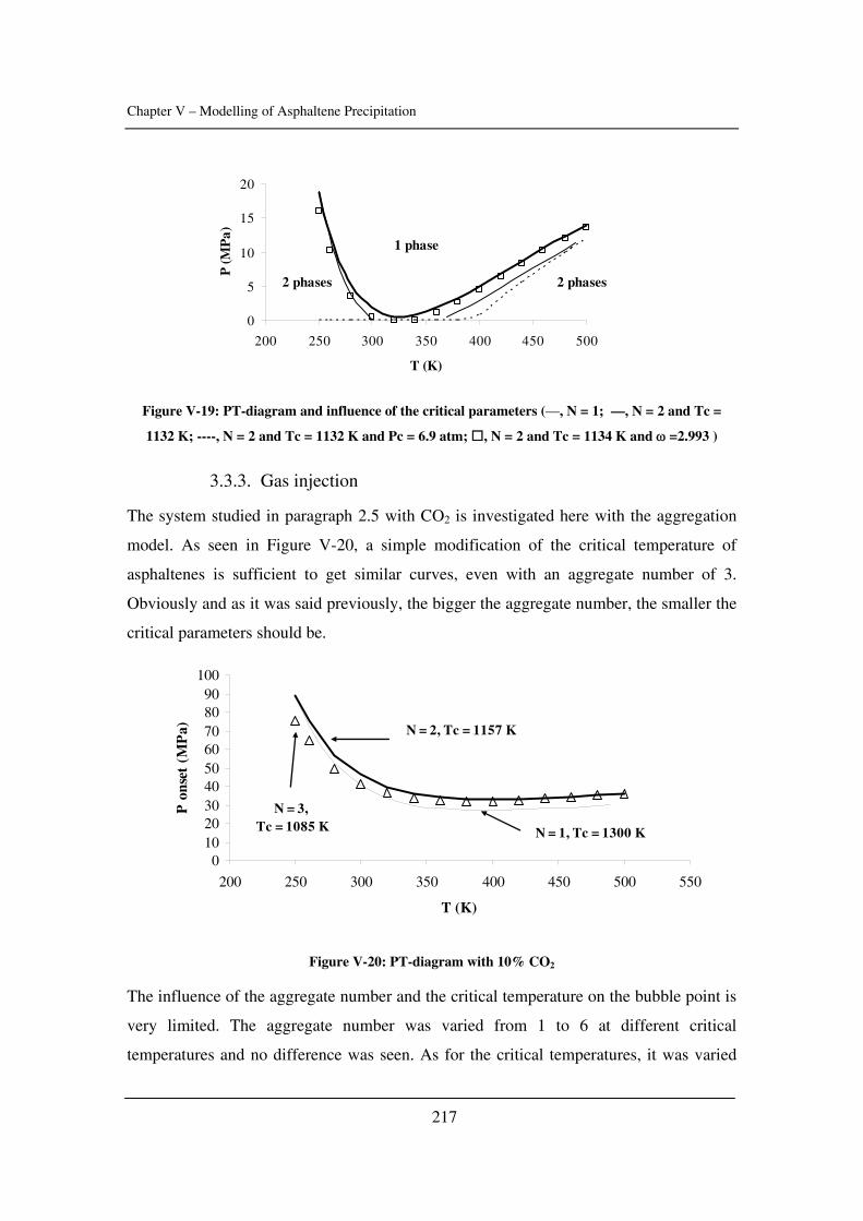
Chapter V – Modelling of Asphaltene Precipitation
217
0
5
10
15
20
200 250 300 350 400 450 500
T (K)
P (M
Pa)
2 phases 2 phases
1 phase
Figure V-19: PT-diagram and influence of the critical parameters (—, N = 1; —, N = 2 and Tc =
1132 K; ----, N = 2 and Tc = 1132 K and Pc = 6.9 atm; , N = 2 and Tc = 1134 K and ω =2.993 )
3.3.3. Gas injection
The system studied in paragraph 2.5 with CO2 is investigated here with the aggregation
model. As seen in Figure V-20, a simple modification of the critical temperature of
asphaltenes is sufficient to get similar curves, even with an aggregate number of 3.
Obviously and as it was said previously, the bigger the aggregate number, the smaller the
critical parameters should be.
0102030405060708090
100
200 250 300 350 400 450 500 550
T (K)
P o
nset
(M
Pa) N = 2, Tc = 1157 K
N = 1, Tc = 1300 K
N = 3, Tc = 1085 K
Figure V-20: PT-diagram with 10% CO2
The influence of the aggregate number and the critical temperature on the bubble point is
very limited. The aggregate number was varied from 1 to 6 at different critical
temperatures and no difference was seen. As for the critical temperatures, it was varied
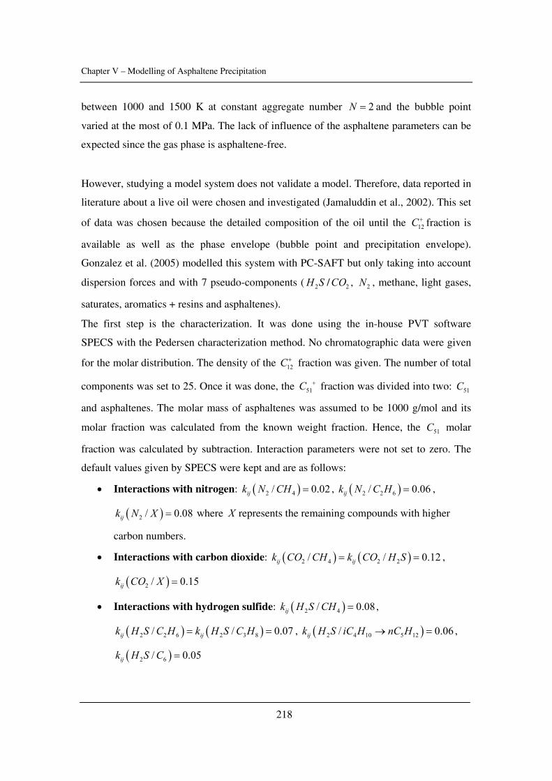
Chapter V – Modelling of Asphaltene Precipitation
218
between 1000 and 1500 K at constant aggregate number 2N = and the bubble point
varied at the most of 0.1 MPa. The lack of influence of the asphaltene parameters can be
expected since the gas phase is asphaltene-free.
However, studying a model system does not validate a model. Therefore, data reported in
literature about a live oil were chosen and investigated (Jamaluddin et al., 2002). This set
of data was chosen because the detailed composition of the oil until the 12C+ fraction is
available as well as the phase envelope (bubble point and precipitation envelope).
Gonzalez et al. (2005) modelled this system with PC-SAFT but only taking into account
dispersion forces and with 7 pseudo-components ( 2H S / 2CO , 2N , methane, light gases,
saturates, aromatics + resins and asphaltenes).
The first step is the characterization. It was done using the in-house PVT software
SPECS with the Pedersen characterization method. No chromatographic data were given
for the molar distribution. The density of the 12C+ fraction was given. The number of total
components was set to 25. Once it was done, the 51C + fraction was divided into two: 51C
and asphaltenes. The molar mass of asphaltenes was assumed to be 1000 g/mol and its
molar fraction was calculated from the known weight fraction. Hence, the 51C molar
fraction was calculated by subtraction. Interaction parameters were not set to zero. The
default values given by SPECS were kept and are as follows:
• Interactions with nitrogen: ( )2 4/ 0.02ijk N CH = , ( )2 2 6/ 0.06ijk N C H = ,
( )2 / 0.08ijk N X = where X represents the remaining compounds with higher
carbon numbers.
• Interactions with carbon dioxide: ( ) ( )2 4 2 2/ / 0.12ij ijk CO CH k CO H S= = ,
( )2 / 0.15ijk CO X =
• Interactions with hydrogen sulfide: ( )2 4/ 0.08ijk H S CH = ,
( ) ( )2 2 6 2 3 8/ / 0.07ij ijk H S C H k H S C H= = , ( )2 4 10 5 12/ 0.06ijk H S iC H nC H→ = ,
( )2 6/ 0.05ijk H S C =
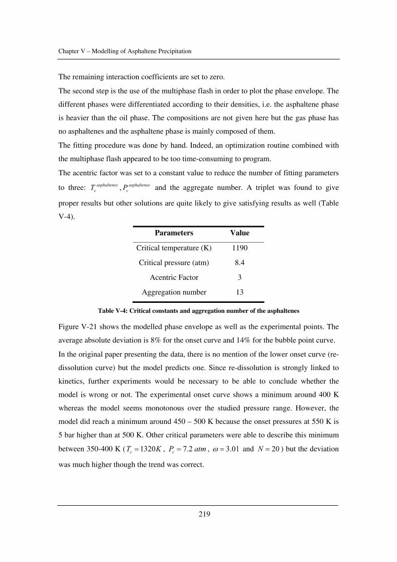
Chapter V – Modelling of Asphaltene Precipitation
219
The remaining interaction coefficients are set to zero.
The second step is the use of the multiphase flash in order to plot the phase envelope. The
different phases were differentiated according to their densities, i.e. the asphaltene phase
is heavier than the oil phase. The compositions are not given here but the gas phase has
no asphaltenes and the asphaltene phase is mainly composed of them.
The fitting procedure was done by hand. Indeed, an optimization routine combined with
the multiphase flash appeared to be too time-consuming to program.
The acentric factor was set to a constant value to reduce the number of fitting parameters
to three: asphaltenescT , asphaltenes
cP and the aggregate number. A triplet was found to give
proper results but other solutions are quite likely to give satisfying results as well (Table
V-4).
Parameters Value
Critical temperature (K) 1190
Critical pressure (atm) 8.4
Acentric Factor 3
Aggregation number 13
Table V-4: Critical constants and aggregation number of the asphaltenes
Figure V-21 shows the modelled phase envelope as well as the experimental points. The
average absolute deviation is 8% for the onset curve and 14% for the bubble point curve.
In the original paper presenting the data, there is no mention of the lower onset curve (re-
dissolution curve) but the model predicts one. Since re-dissolution is strongly linked to
kinetics, further experiments would be necessary to be able to conclude whether the
model is wrong or not. The experimental onset curve shows a minimum around 400 K
whereas the model seems monotonous over the studied pressure range. However, the
model did reach a minimum around 450 – 500 K because the onset pressures at 550 K is
5 bar higher than at 500 K. Other critical parameters were able to describe this minimum
between 350-400 K ( 1320cT K= , 7.2cP atm= , 3.01ω = and 20N = ) but the deviation
was much higher though the trend was correct.
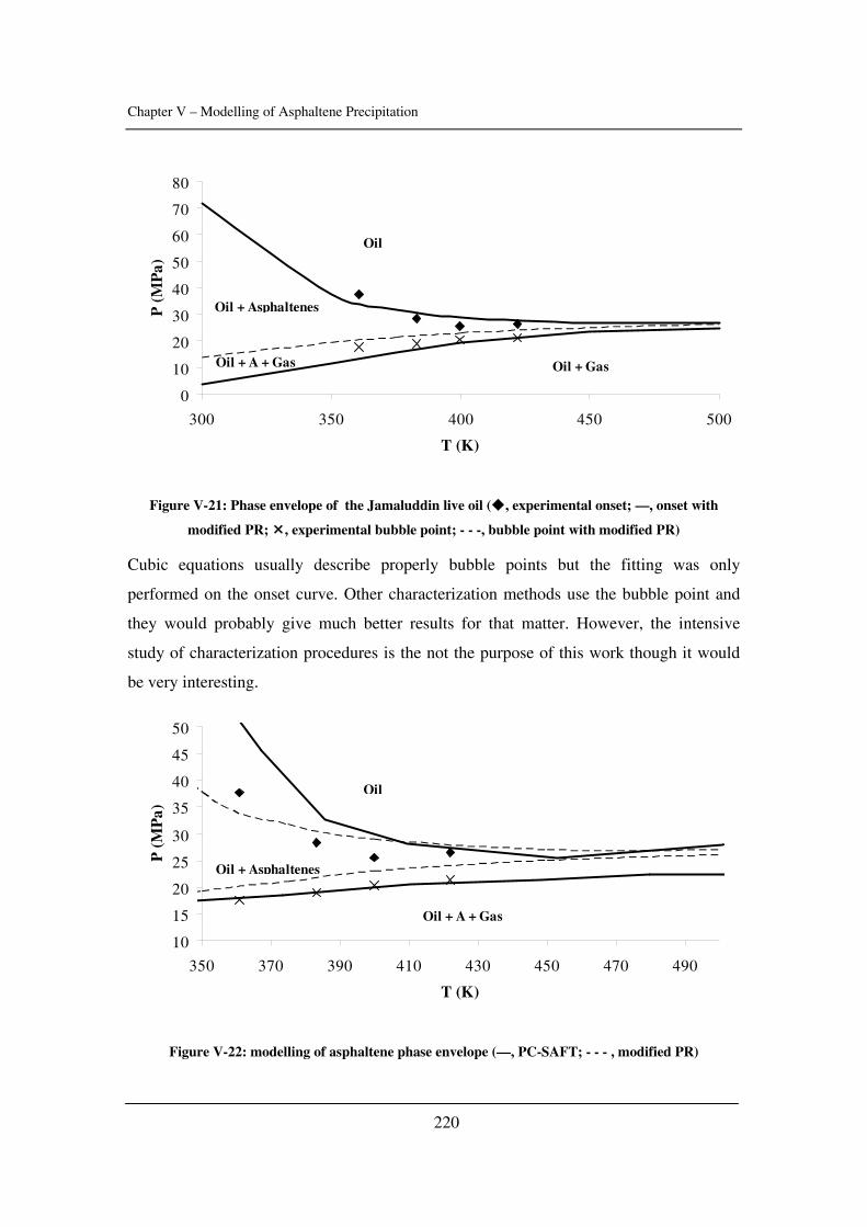
Chapter V – Modelling of Asphaltene Precipitation
220
0
10
20
30
40
50
60
70
80
300 350 400 450 500
T (K)
P (
MP
a)
Oil + Asphaltenes
Oil
Oil + A + Gas Oil + Gas
Figure V-21: Phase envelope of the Jamaluddin live oil ( , experimental onset; —, onset with
modified PR; , experimental bubble point; - - -, bubble point with modified PR)
Cubic equations usually describe properly bubble points but the fitting was only
performed on the onset curve. Other characterization methods use the bubble point and
they would probably give much better results for that matter. However, the intensive
study of characterization procedures is the not the purpose of this work though it would
be very interesting.
10
15
20
25
30
35
40
45
50
350 370 390 410 430 450 470 490
T (K)
P (
MP
a)
Oil + Asphaltenes
Oil
Oil + A + Gas
Figure V-22: modelling of asphaltene phase envelope (—, PC-SAFT; - - - , modified PR)
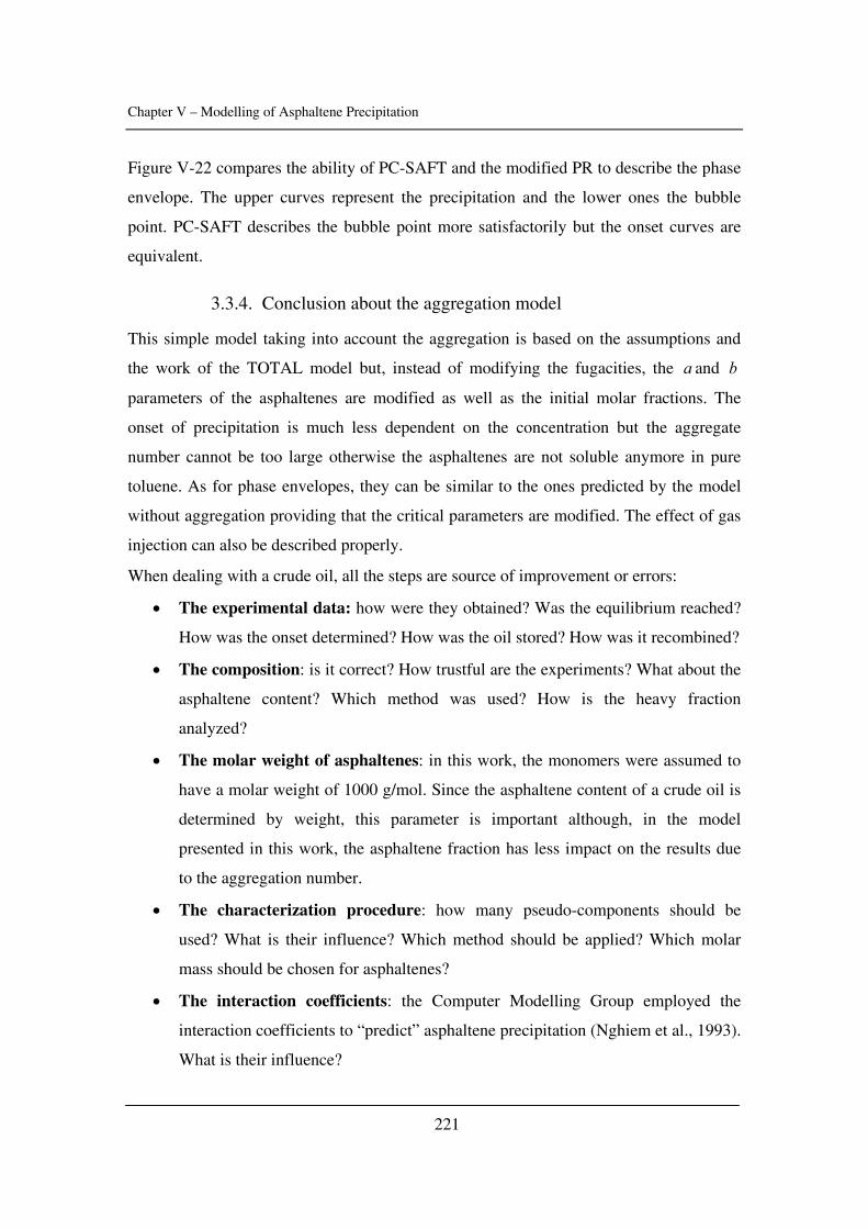
Chapter V – Modelling of Asphaltene Precipitation
221
Figure V-22 compares the ability of PC-SAFT and the modified PR to describe the phase
envelope. The upper curves represent the precipitation and the lower ones the bubble
point. PC-SAFT describes the bubble point more satisfactorily but the onset curves are
equivalent.
3.3.4. Conclusion about the aggregation model
This simple model taking into account the aggregation is based on the assumptions and
the work of the TOTAL model but, instead of modifying the fugacities, the a and b
parameters of the asphaltenes are modified as well as the initial molar fractions. The
onset of precipitation is much less dependent on the concentration but the aggregate
number cannot be too large otherwise the asphaltenes are not soluble anymore in pure
toluene. As for phase envelopes, they can be similar to the ones predicted by the model
without aggregation providing that the critical parameters are modified. The effect of gas
injection can also be described properly.
When dealing with a crude oil, all the steps are source of improvement or errors:
• The experimental data: how were they obtained? Was the equilibrium reached?
How was the onset determined? How was the oil stored? How was it recombined?
• The composition: is it correct? How trustful are the experiments? What about the
asphaltene content? Which method was used? How is the heavy fraction
analyzed?
• The molar weight of asphaltenes: in this work, the monomers were assumed to
have a molar weight of 1000 g/mol. Since the asphaltene content of a crude oil is
determined by weight, this parameter is important although, in the model
presented in this work, the asphaltene fraction has less impact on the results due
to the aggregation number.
• The characterization procedure: how many pseudo-components should be
used? What is their influence? Which method should be applied? Which molar
mass should be chosen for asphaltenes?
• The interaction coefficients: the Computer Modelling Group employed the
interaction coefficients to “predict” asphaltene precipitation (Nghiem et al., 1993).
What is their influence?

Chapter V – Modelling of Asphaltene Precipitation
222
• The fitting procedure: since it was done by hand in this work, the model can
obviously give better results with a proper fitting. Are there any “empirical rules”
linking cT , cP , ω and N ?
If one seriously considers these few items, the words “prediction of asphaltene
precipitation” merely sound utopian.
Chapter V – Modelling of Asphaltene Precipitation
223
4. Conclusion
Asphaltene modelling has been quite intensive since the 80’s. Many different
approaches have been tried. The thermodynamic approach seems to be the appropriate
one since it has strong experimental evidences.
The regular solution is simple and intuitive to use. All possible effects of
temperature and pressure can be described depending on the input parameters of
asphaltenes.
The cubic EOS describe properly phase envelopes but the behaviour with respect to
dilution cannot be predicted.
The TOTAL model brings important improvements thanks to the aggregation
number but, unfortunately, the modified fugacities do not seem to pass the consistency
tests. However, using the same assumptions and only modifying the a and b parameters
of asphaltenes, interesting results can be found such as a much lower dependence to
dilution. This modification helps describing phase envelopes, providing that the critical
parameters of asphaltenes are modified. Literature data were successfully fitted (within
10%) and the model is believed to perform better with a proper fitting procedure.
However, the sources of potential errors and “adjustments” are plethora and they
make modelling a fragile tool with today’s knowledge and understanding of asphaltenes.
Chapter V – Modelling of Asphaltene Precipitation
224
Literature
Alboudwarej H., Akbarzadeh K., Beck J., Svrcek W.Y., Yarranton H.W., Regular Solution Model for Asphaltene Precipitation from Bitumens and Solvents, AIChE J. (2003), 49, 2948 – 2956 Andersen S.I., Speight J.G., Thermodynamic models for asphaltene solubility and precipitation, J. Petrol. Sci. Eng. (1999), 22, 53 - 66 Barton, A.F.M. CRC Handbook of solubility parameters and other cohesion parameters; CRC Press, 1991 Buenrostro-Gonzalez E., Lira-Galeana C., Gil-Villegas A., Wu J., Asphaltene precipitation in crude oils: theory and experiments, AIChE J. (2004), 50, 2552 - 2570 Cimino R., Correra S., Del Bianco A., Lockart T.P., Solubility and Phase Behaviour of asphaltenes in hydrocarbon media, Asphaltenes: Fundamentals and Applications, Sheu E.Y., Mullins O.C., Ed., Plenum Press, NY, 97 - 130 (1995) Christensen A.A., Hadsbjerg C., Vestager-Tybjerg P.C., A study of the perturbed chain statistical associating fluid theory, Midterm Project: Technical University of Denmark, Department of Chemical Engineering, 2005 Diallo M.S., Strachan A., Faulon J.L., Goddard III W.A., Pet. Sci. Technol. (2004), 22, 877 – 899 Fahim M.A., Al-Sahhaf T.A., Elkilani A.S., Prediction of asphaltene precipitation for Kuwaiti crude using thermodynamic micellization model, Ind. Eng. Chem. Res. (2001), 40, 2748 – 2756 Fahim M.A., Andersen S.I., Tuning EOS Using Molecular Thermodynamics to Construct Asphaltene Deposition Envelope (ADE), Presented at the 6th International Conference on Petroleum Phase Behaviour and Fouling, Amsterdam, 2005 Griffith M.G., Siegmund C.W., Controlling compatibility of residual fuels oils, Marine Fuels (1985), 227 – 247 Gonzalez, D. L., Ting, P. D., Hirasaki, G. J., Chapman W.G., Prediction of Asphaltene Instability under Gas Injection with the PC-SAFT Equation of State, Energ. Fuel. (2005), 19, 1230 – 1234 Gupta A.K., A model for asphaltene flocculation using an equation of state, Master thesis, Department of Chemical and Petroleum Engineering, University of Calgary, 1986
Chapter V – Modelling of Asphaltene Precipitation
225
Hansen C.M., Hansen Solubility Parameters: a user’s Handbook, CRC press, 2000 Heidemann R.A., Prausnitz J.M., A van der Waals-type equation of state for fluids with asociating molecules, Proc. Natl. Acad. Sci. (1976), 73, 6, 1773 - 1776 Hirschberg A., deJong L.N.J., Schipper B.A., Meijer J.G., Influence of temperature and Pressure on asphaltene flocculation, paper SPE 11202, SPE J. (1984), 283 – 293 Jamaluddin, A.K.M., Joshi, N., Iwere, F., Gurpinar, O., An investigation of asphaltene instability under nitrogen injection, Proceedings of the SPE International Petroleum Conference and Exhibition of Mexico (2002), 427 – 436 Kawanaka S., Park S.J., Mansoori G.A., Organic deposition from reservoir fluids: a thermodynamic predictive technique, SPE Reservoir Eng. (1991), 6, 185-192 Kontogeorgis G.M., Voutsas E.C., Yakoumis I. V., Tassios D.P., Equation of state for associating fluids, Ind. Eng. Chem. Res. (1996), 35, 4310 - 4318 Knudsen L., Modelling of asphaltene precipitation, Master Thesis, Department if Chemical Engineering, Technical University of Denmark, 2001 Leontaritis K.J., Mansoori G.A., Asphaltene Flocculation during oil recovery and processing: a thermodynamic-colloidal model, SPE paper 16258, SPE International Symposium on Oilfield Chemistry, 4-6 February, San Antonio, Texas (1987) Li M., Guo P., Li S., Modeling technique of asphaltene precipitation, SPE 70048 (2001) Michelsen M., Møllerup J., Thermodynamic models: fundamentals and computational aspects, Tie-Line Publications, Holte, 2004 Michelsen M., Personal communication (2006) Nghiem L.X., Hassam M.S., Nutakki R., George A.E.D., Efficient modelling of asphaltene precipitation, SPE 26642 (1993) Porte G., Zhou H., Lazzeri V., Reversible description of asphaltene colloidal association and precipitation, Langmuir (2003), 19, 40 – 47 Rassamdana H., Dabir B., Nematy M., Farhani M., Sahimi M., Asphalt flocculation and deposition: I. The onset of precipitation, AIChE J. (1996), 42, 1, 10 - 22 Rogel E., Carbognani L., Density estimation of asphaltenes using molecular dynamic simulations, Energ. Fuel. (2003), 17, 378 – 386
Chapter V – Modelling of Asphaltene Precipitation
226
Rogel E., Leon O., Contreras E., Carbognani L., Torres G., Espidel J., Zambrano A., Assesment of asphaltene stability in crude oils using conventionnal techniques, Energ. Fuel. (2003), 17, 1583 – 1590 Szewczyk V., Behar E., Compositional model for predicting asphaltenes flocculation, Fluid Phase Equilibr. (1999), 158, 459 – 469 Ting P.D., Hirasaki G.J., Chapman W.G., Modeling of asphaltene precipitation phase behaviour with the SAFT Equation of state, Pet. Sci. Technol. (2003), 21, 647 - 661 Verdier S., Andersen S.I., Determination of isobaric thermal expansivity of organic compounds from 0.1 to 30 MPa at 30 °C with an isothermal pressure scanning microcalorimeter, J. Chem. Eng. Data 48 (2003), 892 – 897 Verdier S., Andersen S.I., Internal pressure and solubility parameter as a function of pressure, Fluid Phase Equilib. 231 (2005), 125 – 137 Victorov A.I., Firoozabadi A., Thermodynamic micellization model of asphaltene from petroleum fluids, AIChE J. (1996), 42, 1753-1764 Wu J., Prausnitz J.M., Firoozabadi A, Molecular-thermodynamic framework for asphaltene-oil equilibria, AIChE J. (1998), 44, 5, 1188 - 1199 Wu J., Prausnitz J.M., Firoozabadi A., Molecular thermodynamics of asphaltene precipitation in reservoir fluids, AIChE J. (2000), 46, 1, 197 – 209 Zhou H., Total, Personal Communication (2005) Zhou H., Porte G., V. Lazzeri, Personnal Communication (2005)
Chapter V – Modelling of Asphaltene Precipitation
227
List of symbols
Latin letters
a Attractive term of a cubic EOS
ia Activity of compound i
b Co-volume
f Fugacity
G Gibbs energy
ijk Interaction parameter
K Equilibrium constant
m Temperature dependence of the solubility parameter
m Mass
n Mole number
N Aggregation number
sN Number of binding sites
P Pressure
R Gas constant
T Temperature
v Mole volume
x Molar fraction
Z Compressibility Factor
Greek letters
Pα Isobaric thermal expansivity
γ Activity coefficient
δ Solubility Parameter
Tκ Isothermal compressibility
Chapter V – Modelling of Asphaltene Precipitation
228
μ Chemical potential
iv Stoichiometric coefficient of compound i
ρ Density
ϕ Volume fraction
ϕ Fugacity coefficient
χ Interaction parameter
ω Acentric factor
Subscripts and Superscripts
a Asphaltene
agg Aggregates
c Critical
CR Critical
l Liquid
r Reaction
0 Reference/Standard

Chapter VI– Conclusion and Future Challenges
229
Chapter VI
Conclusion and Future Challenges
Chapter VI– Conclusion and Future Challenges
230
Table of Contents
1. Conclusion ............................................................................................................. 231
1.1. Solubility parameter........................................................................................ 231
1.2. Characterization of crude oils ......................................................................... 231
1.3. Solubility parameters of asphaltenes .............................................................. 232
1.4. Critical constants of asphaltenes ..................................................................... 232
1.5. Asphaltene stability and gas injection............................................................. 232
1.6. Asphaltene Stability and Calorimetry............................................................. 233
1.7. Modelling of asphaltene precipitation ............................................................ 233
2. Future Challenges ................................................................................................. 234
2.1. Characterization of crude oils and asphaltenes ............................................... 234
2.2. Asphaltene Stability and gas injection............................................................ 234
2.3. Asphaltene precipitation and calorimetry ....................................................... 235
2.4. Modelling of asphaltene precipitation ............................................................ 235
2.5. Other studies ................................................................................................... 236
Literature....................................................................................................................... 237
Chapter VI– Conclusion and Future Challenges
231
1. Conclusion
This work aimed at getting more understanding about asphaltene stability especially in
presence of gas. This section will summarize the different investigations and the main
results.
1.1. Solubility parameter
Its definition was clarified. If pressure and temperature are to be taken into account,
cohesive energy should be equal to the residual internal energy. The diversity of
definitions in the literature induced many databases and, even for pure compounds,
deviations up to 0.5 MPa1/2 are common. The effect of temperature was studied in the
literature. However, the definitions of cohesive energy highly influence the impact of
temperature. It was tested with a cubic EOS on n-heptane, ethanol and toluene. On the
contrary, the effect of pressure is not well studied in the literature. Pressure was found to
influence cohesive energy and it should therefore be regarded as an important factor.
Cubic EOS combined with experimental volumes turned out to calculate the total
solubility parameter and not the sole dispersion term, as it was expected.
1.2. Characterization of crude oils
The solubility parameter of crude oils was measured using an alternative approach taking
pressure into account: the internal pressure. It is determined indirectly with density
measurements and scanning transitiometry. Pure compounds were investigated at 303.15
K and up to 30 MPa. An accuracy of 1 MPa1/2 was found for hydrocarbons. It was also
confirmed that internal pressure does not “measure” hydrogen bonding. This method was
successfully applied to both dead and live oils. However, the accuracy required by
modelling (0.1 MPa1/2) could not be satisfied. The uncertainty of isothermal
compressibility measurements is the main source of such a high deviation. The high-
pressure calorimetry measurements also confirmed that bubble point can be determined
by scanning transitiometry.
Chapter VI– Conclusion and Future Challenges
232
1.3. Solubility parameters of asphaltenes
A technique based on the regular solution theory and density measurements was applied
to asphaltene solutions. Solubility parameters of two asphaltenes were determined at
303.15 K and 0.1 MPa. Three pairs of solvents were tested and one did not give
satisfactory results. An average deviation of 0.4 MPa1/2 was found. The dependence of
aδ with respect to temperature could be investigated and would be quite easy from an
experimental point of view. The only required parameters would be the internal pressures
and the solubility parameters of the solvents at the studied temperature. As for the
dependence with pressure, larger samples would be necessary since the ISCO pump
should be used.
1.4. Critical constants of asphaltenes
A novel approach using partial volumes and a cubic EOS was tested on asphaltene
solutions. Partial volumes of asphaltenes are measured in three different solvents. Partial
volume calculations are performed with a cubic EOS using the measured densities as
inputs. The calculated and experimental partial volumes are fitted using the critical
constants as adjustable parameters. The ability of this method to evaluate critical
parameters is too poor for modelling (13% of deviation for pure compounds). A second
technique based on NMR data was tested. The content in hetero-atom and the molar
weight have a very strong influence on the calculated critical constants.
1.5. Asphaltene stability and gas injection
A novel high-pressure PVT cell developed at the University of Pau (France) was tested
on several crude oils in presence of carbon dioxide and methane. The onset of
precipitation was determined using isobaric filtration. The influences of pressure and
temperature were determined. Temperature destabilized both crude oils with carbon
dioxide. As for methane, its influence was tested on one crude oil only and temperature
had a stabilizing impact. For all the systems studied, the higher the pressure, the more
soluble the asphaltenes. Reversibility was detected for one crude oil only. The role of
kinetics in such measurements has to be carefully studied though.
Chapter VI– Conclusion and Future Challenges
233
1.6. Asphaltene Stability and Calorimetry
Isothermal titration calorimetry was applied to asphaltene solutions and to crude oils.
Precipitation induced by n-alkanes had no strong thermal effects. It seems that the energy
of the broken bonds (asphaltene-solvent) is equivalent to the one of the created ones
(asphaltene-asphaltene and solvent-solvent). As for precipitation caused by pressure
depletion or by a variation of temperature, it had visible exothermic effects accompanied
by an increase in apparent thermal expansivity (i.e. an increase in volume due to the
creation of a new phase). It is similar to a second-order transition.
1.7. Modelling of asphaltene precipitation
Once the different models used in the literature had been listed, a cubic EOS was tested.
The impact of critical parameters on the asphaltene precipitation curve was investigated.
It confirmed that even a modification of 1% had a strong influence. A simple model
taking into account aggregation and based on cubic EOS was tested. A reported
asphaltene phase envelope could be successfully described. However, the determination
of critical parameters and the potential sources of error and adjustments are so large that
modelling of asphaltene fluid is not predictive with today’s knowledge of asphaltenes.
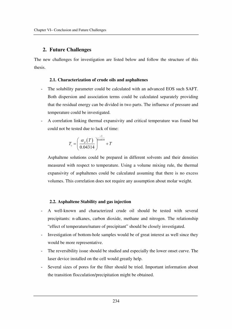
Chapter VI– Conclusion and Future Challenges
234
2. Future Challenges
The new challenges for investigation are listed below and follow the structure of this
thesis.
2.1. Characterization of crude oils and asphaltenes
- The solubility parameter could be calculated with an advanced EOS such SAFT.
Both dispersion and association terms could be calculated separately providing
that the residual energy can be divided in two parts. The influence of pressure and
temperature could be investigated.
- A correlation linking thermal expansivity and critical temperature was found but
could not be tested due to lack of time:
( )1
0.6410
0.04314p
c
TT T
α−
⎛ ⎞= +⎜ ⎟⎝ ⎠
Asphaltene solutions could be prepared in different solvents and their densities
measured with respect to temperature. Using a volume mixing rule, the thermal
expansivity of asphaltenes could be calculated assuming that there is no excess
volumes. This correlation does not require any assumption about molar weight.
2.2. Asphaltene Stability and gas injection
- A well-known and characterized crude oil should be tested with several
precipitants: n-alkanes, carbon dioxide, methane and nitrogen. The relationship
“effect of temperature/nature of precipitant” should be closely investigated.
- Investigation of bottom-hole samples would be of great interest as well since they
would be more representative.
- The reversibility issue should be studied and especially the lower onset curve. The
laser device installed on the cell would greatly help.
- Several sizes of pores for the filter should be tried. Important information about
the transition flocculation/precipitation might be obtained.
Chapter VI– Conclusion and Future Challenges
235
- The effect of nitrogen on asphaltene stability should be studied since it is reported
as a precipitant.
2.3. Asphaltene precipitation and calorimetry
- The influence of the liquid in the reference cell should be investigated for the ITC
experiments (mixtures toluene/heptane could be tried).
- ITC experiments should go on with more oils and asphaltene solutions. Higher
precipitant contents should be tried.
- As for the model systems, well-known sterically stabilised colloids should be
investigated. The signal obtained by flocculation of well-known systems would
probably help interpreting the signals obtained with asphaltenes.
- The effect of temperature could be investigated.
- The HP calorimetry experiments should be combined with the filtration technique
in order to have fewer doubts about the measured signals. It might be possible to
establish a relationship between heat of precipitation and stability with respect to
temperature.
2.4. Modelling of asphaltene precipitation
- The fitting procedure to obtain the critical constants and the aggregation number
should be optimized.
- The influence of the characterization method should be tested.
- A model taking into account polydispersity should be studied since there is not a
single aggregation number but a distribution.
- Critical parameters could be obtained by fitting titration experiments at
atmospheric conditions on a dead oil. They could also be determined with the
method developed in this work and compared to the ones fitted by the EOS. Then,
the APE should be plotted and compared to the experimental one.
Chapter VI– Conclusion and Future Challenges
236
- Aggregation could be modelled as chemical reaction equilibrium following the
recommendations given by Michelsen and Mollerup (2004). Then, this model
may be combined with a multiphase flash.
2.5. Other studies
- SANS and SAXS should be applied to asphaltene solutions next to the onset of
flocculation and precipitation.
- The influence of pressure and temperature on the state of aggregation should be
followed by microscopy and image analysis.
- Precipitation by pressure depletions should be investigated in an accurate high-
pressure pycnometer since there seems to be a change in volumetric properties.
- The size distribution is of interest, especially close to the onsets of flocculation
and precipitation.
- APE of live oils could be determined using speed-of-sound following a procedure
already applied to LLE (Lu et al., 1999) and onset of asphaltene precipitation at
room conditions (Carrier et al., 2000).
- The differences between n-heptane induced precipitation and
pressure/temperature-induced precipitation is of major interest. The fitting
procedures in modelling are often based on n-heptane titrations. Then, the model
is applied to live systems. It would be interesting to investigate whether or not
these types of precipitations have a different nature, as the calorimetric studies of
this work give to understand.
- The co-precipitation of waxes with asphaltenes at low temperature was briefly
introduced. An analysis of the filtrate would be necessary to be sure that the onset
of precipitation is only due to asphaltenes.
Chapter VI– Conclusion and Future Challenges
237
Literature
Carrier H., Plantier F., Daridon J.-L., Lagourette B., Lu Z., Acoustic method for measuring asphaltene flocculation in crude oils, J. Pet. Sci. Eng. (2000), 27, 111 - 117 Lu Z., Daridon J.L., Lagourette B., Ye S., Phase comparison technique for measuring liquid-liquid phase equilibrium, Rev. Sci. Instrum. (1999), 70, 2065-2068 Michelsen M.L., Mollerup J.M., Thermodynamic models: fundamentals and computational aspects, Tie-Line Publications, Holte, 2004 Ratzsch M., The calculation of critical temperatures of binary mixtures from thermal expansion coefficient, Chem. Tech.- Leipzig (1969), 21, 774 – 775

Appendixes
Appendixes
Appendixes
List of Appendixes
Appendix I-1: Modified IP 143 method to measure the asphaltene content of a crude oil
Appendix I-2: Intermolecular forces
Appendix II-1: Influence of temperature on the solubility parameters of toluene and
ethanol
Appendix II-2: Influence of pressure on the solubility parameters of toluene and ethanol
Appendix II-3: Relationship between solubility parameter and internal pressure
Appendix II-4: Verdier S., Andersen S.I., Fluid Phase Equilibr. (2005), 231, 125–137
Appendix II-5: Verdier S., Duong D., Andersen S.I., Energ. Fuel. (2005), 19, 1225 –
1229
Appendix II-6: Origin and purity of the chemical compounds used for partial molar
volumes measurements
Appendix II-7: Alexander’s correlations
Appendix II-8: Elemental analysis, Molecular weight and NMR data for various
asphaltenes
Appendix III-1: The Le Châtelier’s Principle
Appendix III-2: Verdier S., Carrier H., Andersen S.I., Daridon J.L., Energ. Fuel. (2006),
to be published
Appendix IV-1: Description procedure ITC
Appendix IV-2: Precipitation of AgCl
Appendix IV-3: Enthalpograms of the precipitation AgCl
Appendix IV-4: Enthalpograms of the precipitation of Boscan solutions
Appendixes
Appendix I-1: Modified IP 143 method to measure the asphaltene content of a crude
oil
Day 1
1. Weigh off 5g oil in 500ml Erlenmeyer glass
2. Add 30ml of n-heptane/g oil and weigh the amount of n-heptane
3. Cover with aluminium foil
4. Blend on ultra sound water bath for 10-15 min.
5. Rest for 16-18 h in darkness
Day 2
1. Transfer the suspended mixture quantitatively to a glass filter (Pyrex ASTM 4-5.5 .F)
with suction and wash with, n-heptane. This is done .by stopping suction, adding ca.
20ml n-heptane, let it be for a couple of minutes and start suction again. Continue till the
washing liquid is colourless.
2. Put the filter on a small- suction flask and heat ca. 40ml toluene. The asphaltenes are
now dissolved similar to the washing process above. Use as small an amount of toluene
as possible.
3. The toluene is removed by rotational evaporation at 80°C.
4. The asphaltenes are transferred to a preparation glass with toluene – max. 10 mL -
remember to tare the preparation glass.
5. The toluene is evaporated in a water bath at 60°C under a flow of nitrogen.
6. To remove the last toluene, the preparation glass is placed in a vacuum oven.
7. A drop of toluene is added to the preparation glass to moisten the asphaltenes and then
10 ml n-heptane are added. Mix on ultra sound bath for 10 min. and centrifuge for 15
min. Remove as much h-heptane as possible without removing any solids. Continue till
liquid is colourless.
8. The asphaltenes are dried in a vacuum oven.
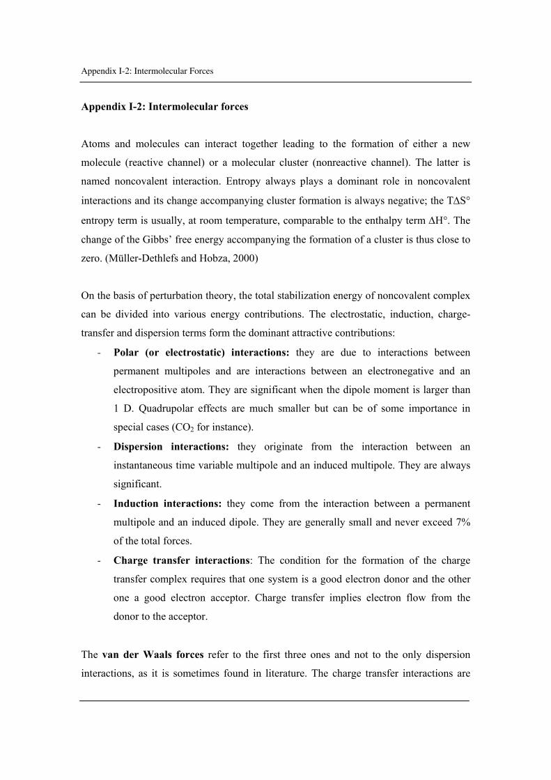
Appendix I-2: Intermolecular Forces
Appendix I-2: Intermolecular forces
Atoms and molecules can interact together leading to the formation of either a new
molecule (reactive channel) or a molecular cluster (nonreactive channel). The latter is
named noncovalent interaction. Entropy always plays a dominant role in noncovalent
interactions and its change accompanying cluster formation is always negative; the TΔS°
entropy term is usually, at room temperature, comparable to the enthalpy term ΔH°. The
change of the Gibbs’ free energy accompanying the formation of a cluster is thus close to
zero. (Müller-Dethlefs and Hobza, 2000)
On the basis of perturbation theory, the total stabilization energy of noncovalent complex
can be divided into various energy contributions. The electrostatic, induction, charge-
transfer and dispersion terms form the dominant attractive contributions:
- Polar (or electrostatic) interactions: they are due to interactions between
permanent multipoles and are interactions between an electronegative and an
electropositive atom. They are significant when the dipole moment is larger than
1 D. Quadrupolar effects are much smaller but can be of some importance in
special cases (CO2 for instance).
- Dispersion interactions: they originate from the interaction between an
instantaneous time variable multipole and an induced multipole. They are always
significant.
- Induction interactions: they come from the interaction between a permanent
multipole and an induced dipole. They are generally small and never exceed 7%
of the total forces.
- Charge transfer interactions: The condition for the formation of the charge
transfer complex requires that one system is a good electron donor and the other
one a good electron acceptor. Charge transfer implies electron flow from the
donor to the acceptor.
The van der Waals forces refer to the first three ones and not to the only dispersion
interactions, as it is sometimes found in literature. The charge transfer interactions are
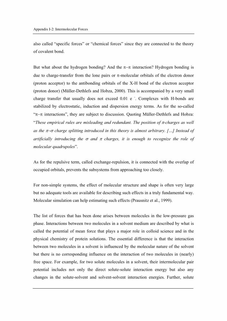
Appendix I-2: Intermolecular Forces
also called “specific forces” or “chemical forces” since they are connected to the theory
of covalent bond.
But what about the hydrogen bonding? And the π−π interaction? Hydrogen bonding is
due to charge-transfer from the lone pairs or π-molecular orbitals of the electron donor
(proton acceptor) to the antibonding orbitals of the X-H bond of the electron acceptor
(proton donor) (Müller-Dethlefs and Hobza, 2000). This is accompanied by a very small
charge transfer that usually does not exceed 0.01 e -. Complexes with H-bonds are
stabilized by electrostatic, induction and dispersion energy terms. As for the so-called
“π−π interactions”, they are subject to discussion. Quoting Müller-Dethlefs and Hobza:
“These empirical rules are misleading and redundant. The position of π-charges as well
as the π−σ charge splitting introduced in this theory is almost arbitrary. […] Instead of
artificially introducing the σ and π charges, it is enough to recognize the role of
molecular quadrupoles”.
As for the repulsive term, called exchange-repulsion, it is connected with the overlap of
occupied orbitals, prevents the subsystems from approaching too closely.
For non-simple systems, the effect of molecular structure and shape is often very large
but no adequate tools are available for describing such effects in a truly fundamental way.
Molecular simulation can help estimating such effects (Prausnitz et al., 1999).
The list of forces that has been done arises between molecules in the low-pressure gas
phase. Interactions between two molecules in a solvent medium are described by what is
called the potential of mean force that plays a major role in colloid science and in the
physical chemistry of protein solutions. The essential difference is that the interaction
between two molecules in a solvent is influenced by the molecular nature of the solvent
but there is no corresponding influence on the interaction of two molecules in (nearly)
free space. For example, for two solute molecules in a solvent, their intermolecular pair
potential includes not only the direct solute-solute interaction energy but also any
changes in the solute-solvent and solvent-solvent interaction energies. Further, solute
Appendix I-2: Intermolecular Forces
molecule often perturbs the local ordering of the solvent molecules. The energy
associated with this perturbation depends on the distance between the two dissolved
molecules and it produces an additional solvation force between them.
References
Müller-Dethlefs K., Hobza K., Noncovalent interactions: a challenge for experiment and
theory, Chem. Rev. (2000), 100, 143 – 167
Prausnitz J.M., Lichtenthaler R.N., Gomes de Azevedo E., Molecular thermodynamics of
Fluid-Phase Equilibria (3rd edition), Prentice Hall PTR, New Jersey, 1999
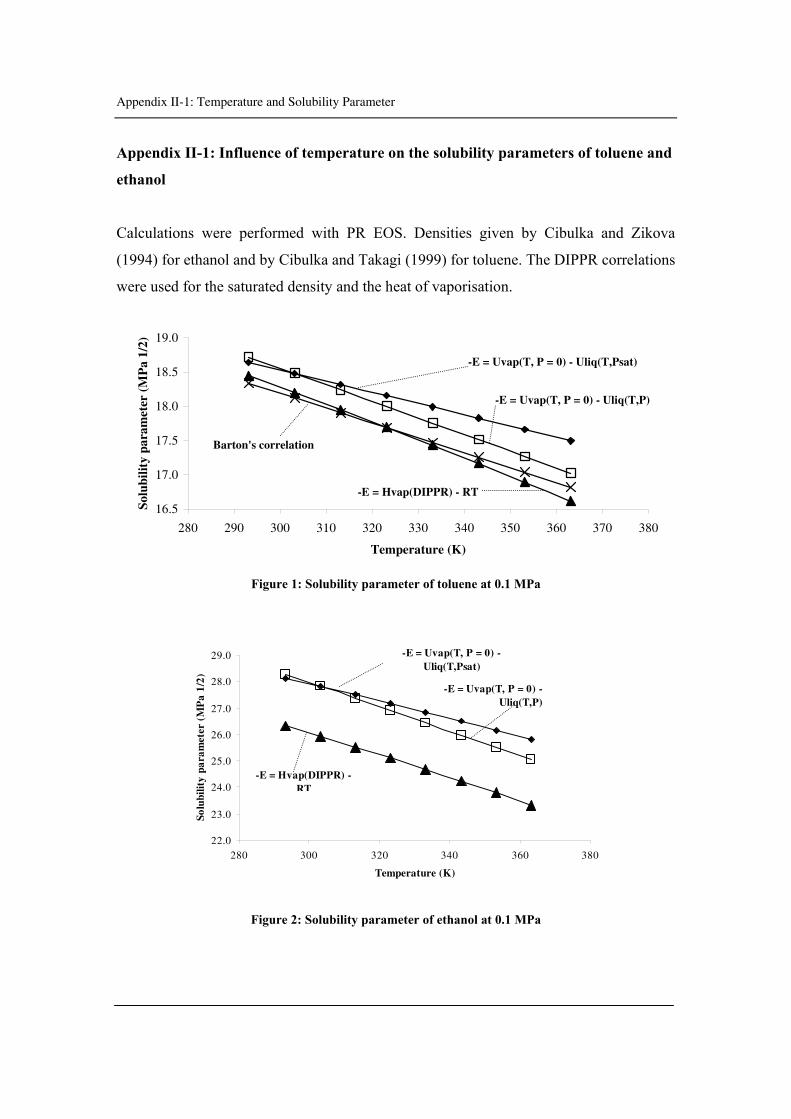
Appendix II-1: Temperature and Solubility Parameter
Appendix II-1: Influence of temperature on the solubility parameters of toluene and
ethanol
Calculations were performed with PR EOS. Densities given by Cibulka and Zikova
(1994) for ethanol and by Cibulka and Takagi (1999) for toluene. The DIPPR correlations
were used for the saturated density and the heat of vaporisation.
16.5
17.0
17.5
18.0
18.5
19.0
280 290 300 310 320 330 340 350 360 370 380
Temperature (K)
Solu
bilit
y pa
ram
eter
(M
Pa
1/2)
-E = Uvap(T, P = 0) - Uliq(T,Psat)
-E = Uvap(T, P = 0) - Uliq(T,P)
Barton's correlation
-E = Hvap(DIPPR) - RT
Figure 1: Solubility parameter of toluene at 0.1 MPa
22.0
23.0
24.0
25.0
26.0
27.0
28.0
29.0
280 300 320 340 360 380
Temperature (K)
Solu
bilit
y pa
ram
eter
(M
Pa
1/2)
-E = Uvap(T, P = 0) - Uliq(T,Psat)
-E = Uvap(T, P = 0) -Uliq(T,P)
-E = Hvap(DIPPR) - RT
Figure 2: Solubility parameter of ethanol at 0.1 MPa

Appendix II-1: Temperature and Solubility Parameter
Cibulka I., Zikova M., Liquid densities at elevated pressures of 1-alkanols from C1 to
C10. A critical evaluation of experimental data, J. Chem. Eng. Data (1994), 39, 876 – 886
Cibulka I., Takagi T., P-rho-T data of liquids: summarization and Evaluation. 5 –
Aromatic hydrocarbons, J. Chem. Eng. Data (1999), 44, 411 - 429
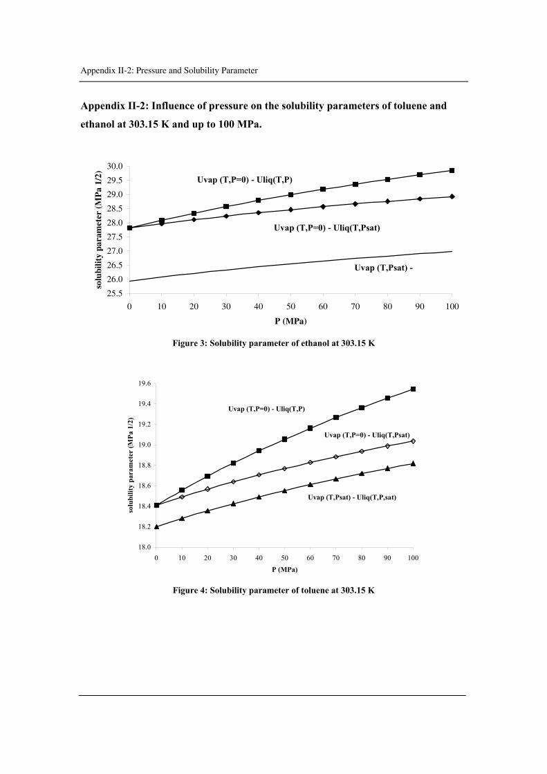
Appendix II-2: Pressure and Solubility Parameter
Appendix II-2: Influence of pressure on the solubility parameters of toluene and
ethanol at 303.15 K and up to 100 MPa.
25.5
26.0
26.5
27.0
27.5
28.0
28.5
29.0
29.5
30.0
0 10 20 30 40 50 60 70 80 90 100
P (MPa)
solu
bilit
y pa
ram
eter
(M
Pa
1/2) Uvap (T,P=0) - Uliq(T,P)
Uvap (T,P=0) - Uliq(T,Psat)
Uvap (T,Psat) -
Figure 3: Solubility parameter of ethanol at 303.15 K
18.0
18.2
18.4
18.6
18.8
19.0
19.2
19.4
19.6
0 10 20 30 40 50 60 70 80 90 100P (MPa)
solu
bilit
y pa
ram
eter
(MPa
1/2
)
Uvap (T,P=0) - Uliq(T,P)
Uvap (T,P=0) - Uliq(T,Psat)
Uvap (T,Psat) - Uliq(T,P,sat)
Figure 4: Solubility parameter of toluene at 303.15 K
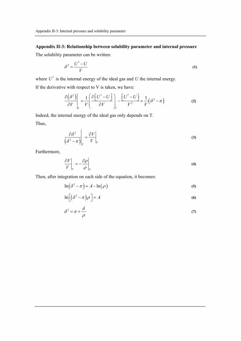
Appendix II-3: Internal pressure and solubility parameter
Appendix II-3: Relationship between solubility parameter and internal pressure
The solubility parameter can be written: *
2 U UV
δ −= (1)
where *U is the internal energy of the ideal gas and U the internal energy.
If the derivative with respect to V is taken, we have:
( ) ( )2 * *
22
1 1
TT
U U U UV V V V Vδ
δ π⎛ ⎞⎡ ⎤ ⎡ ⎤∂ ∂ − −⎣ ⎦ ⎣ ⎦⎜ ⎟= − = −⎜ ⎟∂ ∂⎝ ⎠
(2)
Indeed, the internal energy of the ideal gas only depends on T.
Thus,
( )2
2T
T
VV
δδ π
∂ ∂=
− (3)
Furthermore,
T T
VV
ρρ
∂ ∂= − (4)
Then, after integration on each side of the equation, it becomes:
( ) ( )2ln lnAδ π ρ− = − (5)
( )2ln Aδ π ρ⎡ ⎤− =⎣ ⎦ (6)
'2 Aδ π
ρ= + (7)

Appendix II-4: Verdier and Andersen, 2005
Appendix II-4: Verdier S., Andersen S.I., Internal pressure and solubility
parameter as a function of pressure, Fluid Phase Equilibr. (2005), 231, 125–137

Appendix II-5: Verdier et al., 2005
Appendix 2-5: Verdier S., Duong D., Andersen S.I., Experimental determination of
solubility parameters of oils as function of pressure, Energ. Fuel. (2005), 19, 1225 -
1229
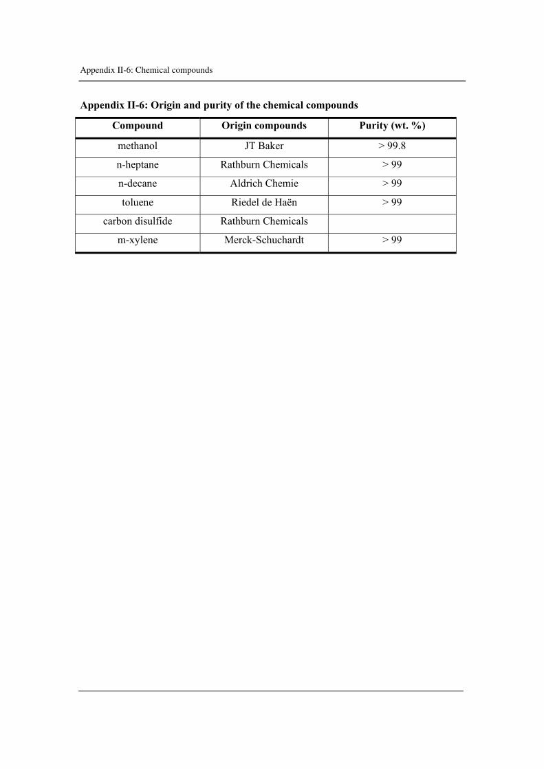
Appendix II-6: Chemical compounds
Appendix II-6: Origin and purity of the chemical compounds
Compound Origin compounds Purity (wt. %)
methanol JT Baker > 99.8
n-heptane Rathburn Chemicals > 99
n-decane Aldrich Chemie > 99
toluene Riedel de Haën > 99
carbon disulfide Rathburn Chemicals
m-xylene Merck-Schuchardt > 99
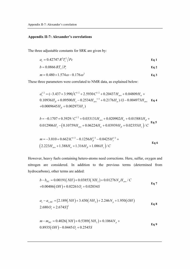
Appendix II-7: Alexander’s correlation
Appendix II-7: Alexander’s correlations
The three adjustable constants for SRK are given by:
2 20.42747c ca R T Pc= Eq 1
0.0866 c cb RT P= Eq 2
20.480 1.574 0.176m ω ω= + − Eq 3
These three parameters were correlated to NMR data, as explained below:
1/ 2 1/ 2 1/ 2
1/ 2
( 3.437 3.990 2.5930 0.20437 0.04809
0.10936 0.09500 0.2534 0.2176 ) /(1 0.0049730.0009645 0.002973 )
c aro
aro aro
a C C H H
H H H H HH H
α
β γ α
β γ
= − + + + + +
+ − + −
+ +
Eq 4
( )
1/ 20.1707 0.3929 / 0.033131 0.020902 0.015881
0.012906 0.10759 0.06224 0.03939 0.02355 /aro
aro
b C H H H
H H H H H Cα β
γ α β γ
= − + + + + +
− + + +Eq 5
( )
1/ 2 1/ 2 1/ 23.010 0.6621 0.1256 0.0425
2.223 1.388 1.316 1.086 /aro
m C H H
H H H H Cβ γ
α β γ
= − + − − +
+ + + Eq 6
However, heavy fuels containing hetero-atoms need corrections. Here, sulfur, oxygen and
nitrogen are considered. In addition to the previous terms (determined from
hydrocarbons), other terms are added:
( ) ( )( )
20.00191 0.03853 0.01276 /
0.00486 0.02261 0.02034HC p aro
e
b b NH NH N H C
OH O S
− = + +
+ + + Eq 7
( ) ( ) ( ), 2
2
[2.189 3.430 2.246 1.950
2.680 2.674 ]c c HC p
e
a a NH NH N OH
O S
− = + + +
+ Eq 8
( ) ( )( )
20.4026 0.5389 0.1064
0.8935 0.0445 0.2545HC p
e
m m NH NH N
OH O S
− = + + +
− + Eq 9
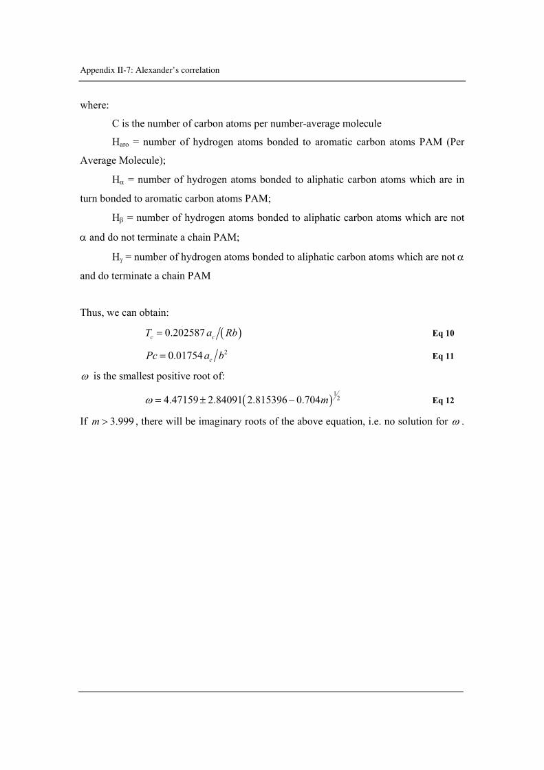
Appendix II-7: Alexander’s correlation
where:
C is the number of carbon atoms per number-average molecule
Haro = number of hydrogen atoms bonded to aromatic carbon atoms PAM (Per
Average Molecule);
Hα = number of hydrogen atoms bonded to aliphatic carbon atoms which are in
turn bonded to aromatic carbon atoms PAM;
Hβ = number of hydrogen atoms bonded to aliphatic carbon atoms which are not
α and do not terminate a chain PAM;
Hγ = number of hydrogen atoms bonded to aliphatic carbon atoms which are not α
and do terminate a chain PAM
Thus, we can obtain:
( )0.202587c cT a Rb= Eq 10
20.01754 cPc a b= Eq 11
ω is the smallest positive root of:
( )1
24.47159 2.84091 2.815396 0.704mω = ± − Eq 12
If 3.999m > , there will be imaginary roots of the above equation, i.e. no solution for ω .
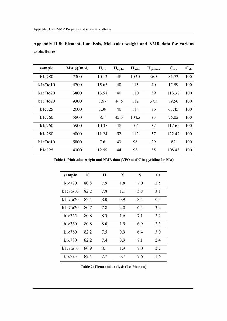
Appendix II-8: NMR Properties of some asphaltenes
Appendix II-8: Elemental analysis, Molecular weight and NMR data for various
asphaltenes
sample Mw (g/mol) Haro Halpha Hbeta Hgamma Caro Cali
b1c780 7300 10.13 48 109.5 36.5 81.73 100
k1c7to10 4700 15.65 40 115 40 17.59 100
k1c7to20 3800 13.58 40 110 39 113.37 100
b1c7to20 9300 7.67 44.5 112 37.5 79.56 100
b1c725 2000 7.39 40 114 36 67.45 100
b1c760 5800 8.1 42.5 104.5 35 76.02 100
k1c760 5900 10.35 48 104 37 112.65 100
k1c780 6800 11.24 52 112 37 122.42 100
b1c7to10 5800 7.6 43 98 29 62 100
k1c725 4300 12.59 44 98 35 108.88 100
Table 1: Molecular weight and NMR data (VPO at 60C in pyridine for Mw)
sample C H N S O
b1c780 80.8 7.9 1.8 7.0 2.5
k1c7to10 82.2 7.8 1.1 5.8 3.1
k1c7to20 82.4 8.0 0.9 8.4 0.3
b1c7to20 80.7 7.8 2.0 6.4 3.2
b1c725 80.8 8.3 1.6 7.1 2.2
b1c760 80.8 8.0 1.9 6.9 2.5
k1c760 82.2 7.5 0.9 6.4 3.0
k1c780 82.2 7.4 0.9 7.1 2.4
b1c7to10 80.9 8.1 1.9 7.0 2.2
k1c725 82.4 7.7 0.7 7.6 1.6
Table 2: Elemental analysis (LeoPharma)
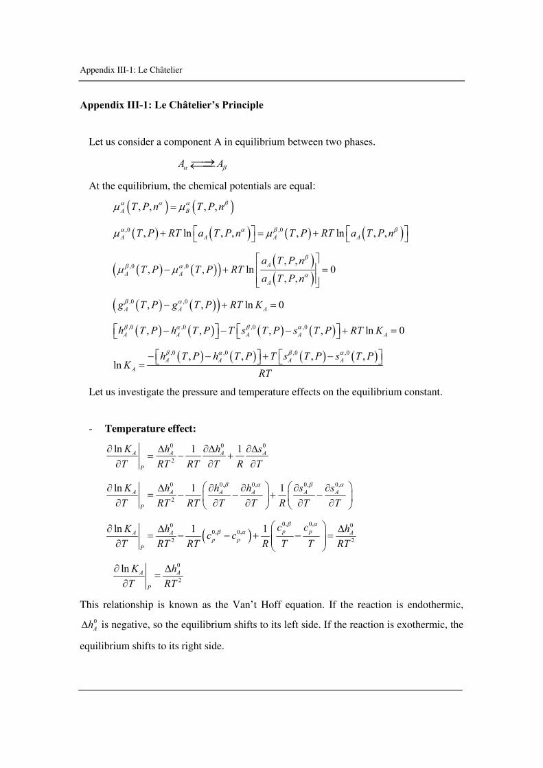
Appendix III-1: Le Châtelier
Appendix III-1: Le Châtelier’s Principle
Let us consider a component A in equilibrium between two phases.
A Aα β⎯⎯→←⎯⎯
At the equilibrium, the chemical potentials are equal:
( ) ( ), , , ,A BT P n T P nα α α βμ μ=
( ) ( ) ( ) ( ),0 ,0, ln , , , ln , ,A A A AT P RT a T P n T P RT a T P nα α β βμ μ⎡ ⎤ ⎡ ⎤+ = +⎣ ⎦ ⎣ ⎦
( ) ( )( ) ( )( )
,0 ,0, ,
, , ln 0, ,
AA A
A
a T P nT P T P RT
a T P n
ββ α
αμ μ
⎡ ⎤⎢ ⎥− + =⎢ ⎥⎣ ⎦
( ) ( )( ),0 ,0, , ln 0A A Ag T P g T P RT Kβ α− + =
( ) ( ) ( ) ( ),0 ,0 ,0 ,0, , , , ln 0A A A A Ah T P h T P T s T P s T P RT Kβ α β α⎡ ⎤ ⎡ ⎤− − − + =⎣ ⎦ ⎣ ⎦
( ) ( ) ( ) ( ),0 ,0 ,0 ,0, , , ,
ln A A A AA
h T P h T P T s T P s T PK
RT
β α β α⎡ ⎤ ⎡ ⎤− − + −⎣ ⎦ ⎣ ⎦=
Let us investigate the pressure and temperature effects on the equilibrium constant.
- Temperature effect:
0 0 0
2
ln 1 1A A A A
P
K h h sT RT RT T R T
∂ Δ ∂Δ ∂Δ= − +
∂ ∂ ∂
0 0, 0, 0, 0,
2
ln 1 1A A A A A A
P
K h h h s sT RT RT T T R T T
β α β α⎛ ⎞ ⎛ ⎞∂ Δ ∂ ∂ ∂ ∂= − − + −⎜ ⎟ ⎜ ⎟∂ ∂ ∂ ∂ ∂⎝ ⎠ ⎝ ⎠
( )0, 0,0 0
0, 0,2 2
ln 1 1 p pA A Ap p
P
c cK h hc cT RT RT R T T RT
β αβ α ⎛ ⎞∂ Δ Δ
= − − + − =⎜ ⎟⎜ ⎟∂ ⎝ ⎠
0
2
ln A A
P
K hT RT
∂ Δ=
∂
This relationship is known as the Van’t Hoff equation. If the reaction is endothermic,
0AhΔ is negative, so the equilibrium shifts to its left side. If the reaction is exothermic, the
equilibrium shifts to its right side.
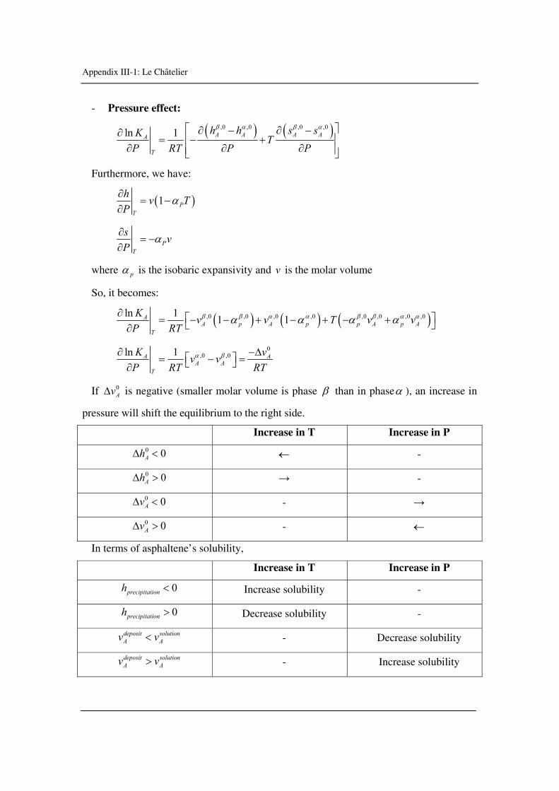
Appendix III-1: Le Châtelier
- Pressure effect:
( ) ( ),0 ,0 ,0 ,0
ln 1 A A A AA
T
h h s sK TP RT P P
β α β α⎡ ⎤∂ − ∂ −∂⎢ ⎥= − +
∂ ∂ ∂⎢ ⎥⎣ ⎦
Furthermore, we have:
( )1 PT
h v TP
α∂= −
∂
PT
s vP
α∂= −
∂
where pα is the isobaric expansivity and v is the molar volume
So, it becomes:
( ) ( ) ( ),0 ,0 ,0 ,0 ,0 ,0 ,0 ,0ln 1 1 1AA p A p p A p A
T
K v v T v vP RT
β β α α β β α αα α α α∂ ⎡ ⎤= − − + − + − +⎣ ⎦∂
0
,0 ,0ln 1A AA A
T
K vv vP RT RT
α β∂ −Δ⎡ ⎤= − =⎣ ⎦∂
If 0AvΔ is negative (smaller molar volume is phase β than in phaseα ), an increase in
pressure will shift the equilibrium to the right side.
Increase in T Increase in P
0 0AhΔ < ← -
0 0AhΔ > → -
0 0AvΔ < - →
0 0AvΔ > - ←
In terms of asphaltene’s solubility,
Increase in T Increase in P
0precipitationh < Increase solubility -
0precipitationh > Decrease solubility -
deposit solutionA Av v< - Decrease solubility
deposit solutionA Av v> - Increase solubility

Appendix III-2: Verdier et al., 2006
Appendix III-2 : Verdier S., Carrier H., Andersen S.I., Daridon J.L., Study of
pressure and temperature effect on asphaltene stability in presence of CO2, Energ.
Fuel. (2006), to be published
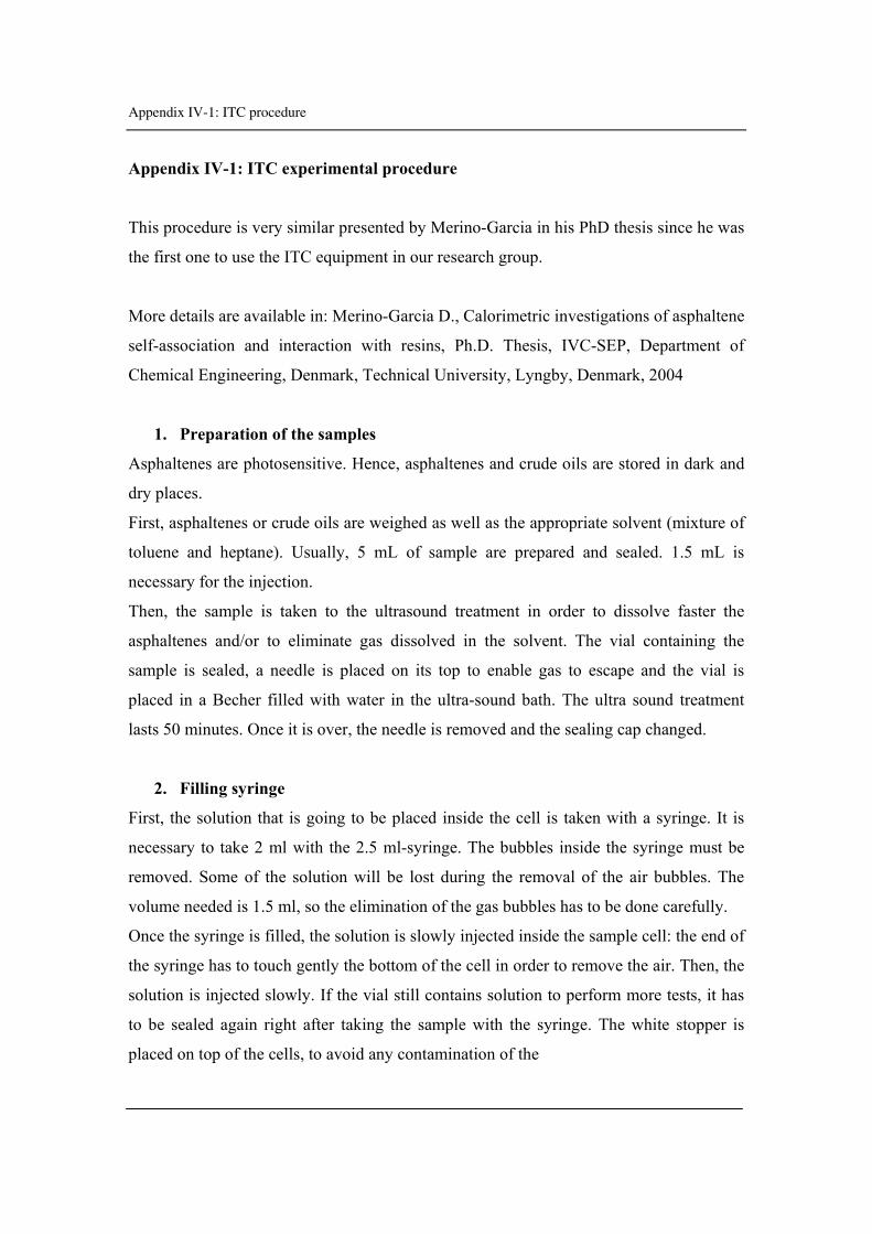
Appendix IV-1: ITC procedure
Appendix IV-1: ITC experimental procedure
This procedure is very similar presented by Merino-Garcia in his PhD thesis since he was
the first one to use the ITC equipment in our research group.
More details are available in: Merino-Garcia D., Calorimetric investigations of asphaltene
self-association and interaction with resins, Ph.D. Thesis, IVC-SEP, Department of
Chemical Engineering, Denmark, Technical University, Lyngby, Denmark, 2004
1. Preparation of the samples
Asphaltenes are photosensitive. Hence, asphaltenes and crude oils are stored in dark and
dry places.
First, asphaltenes or crude oils are weighed as well as the appropriate solvent (mixture of
toluene and heptane). Usually, 5 mL of sample are prepared and sealed. 1.5 mL is
necessary for the injection.
Then, the sample is taken to the ultrasound treatment in order to dissolve faster the
asphaltenes and/or to eliminate gas dissolved in the solvent. The vial containing the
sample is sealed, a needle is placed on its top to enable gas to escape and the vial is
placed in a Becher filled with water in the ultra-sound bath. The ultra sound treatment
lasts 50 minutes. Once it is over, the needle is removed and the sealing cap changed.
2. Filling syringe
First, the solution that is going to be placed inside the cell is taken with a syringe. It is
necessary to take 2 ml with the 2.5 ml-syringe. The bubbles inside the syringe must be
removed. Some of the solution will be lost during the removal of the air bubbles. The
volume needed is 1.5 ml, so the elimination of the gas bubbles has to be done carefully.
Once the syringe is filled, the solution is slowly injected inside the sample cell: the end of
the syringe has to touch gently the bottom of the cell in order to remove the air. Then, the
solution is injected slowly. If the vial still contains solution to perform more tests, it has
to be sealed again right after taking the sample with the syringe. The white stopper is
placed on top of the cells, to avoid any contamination of the
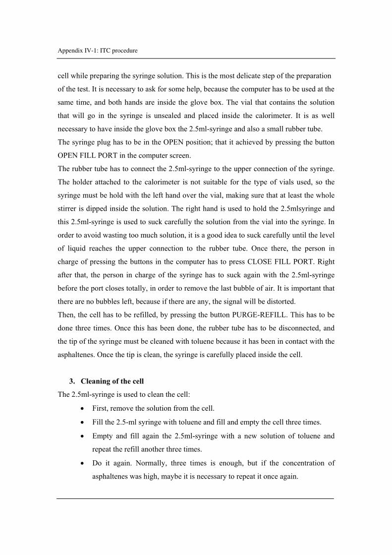
Appendix IV-1: ITC procedure
cell while preparing the syringe solution. This is the most delicate step of the preparation
of the test. It is necessary to ask for some help, because the computer has to be used at the
same time, and both hands are inside the glove box. The vial that contains the solution
that will go in the syringe is unsealed and placed inside the calorimeter. It is as well
necessary to have inside the glove box the 2.5ml-syringe and also a small rubber tube.
The syringe plug has to be in the OPEN position; that it achieved by pressing the button
OPEN FILL PORT in the computer screen.
The rubber tube has to connect the 2.5ml-syringe to the upper connection of the syringe.
The holder attached to the calorimeter is not suitable for the type of vials used, so the
syringe must be hold with the left hand over the vial, making sure that at least the whole
stirrer is dipped inside the solution. The right hand is used to hold the 2.5mlsyringe and
this 2.5ml-syringe is used to suck carefully the solution from the vial into the syringe. In
order to avoid wasting too much solution, it is a good idea to suck carefully until the level
of liquid reaches the upper connection to the rubber tube. Once there, the person in
charge of pressing the buttons in the computer has to press CLOSE FILL PORT. Right
after that, the person in charge of the syringe has to suck again with the 2.5ml-syringe
before the port closes totally, in order to remove the last bubble of air. It is important that
there are no bubbles left, because if there are any, the signal will be distorted.
Then, the cell has to be refilled, by pressing the button PURGE-REFILL. This has to be
done three times. Once this has been done, the rubber tube has to be disconnected, and
the tip of the syringe must be cleaned with toluene because it has been in contact with the
asphaltenes. Once the tip is clean, the syringe is carefully placed inside the cell.
3. Cleaning of the cell
The 2.5ml-syringe is used to clean the cell:
• First, remove the solution from the cell.
• Fill the 2.5-ml syringe with toluene and fill and empty the cell three times.
• Empty and fill again the 2.5ml-syringe with a new solution of toluene and
repeat the refill another three times.
• Do it again. Normally, three times is enough, but if the concentration of
asphaltenes was high, maybe it is necessary to repeat it once again.

Appendix IV-1: ITC procedure
• If the toluene is still not transparent, inject toluene in the cell. Start the ITC
procedure and let the stirring on for a few hours.
• Once it seems clean, dry the cell with air, using the THERMOVAC.
4. Cleaning of the syringe
In the first step, a big vial (20 ml) is placed under the holder of the syringe, making sure
there is enough toluene to cover the tip of the syringe. Press the button CLOSE FILL
PORT (or UP 29 times) to suck the toluene. Press PURGE-REFILL a couple of times.
Change the toluene solution and repeat the same procedure.
Then, press the button OPEN FILL PORT and take the syringe out of the glove box.
Connect the rubber tube to the upper connection and the rubber tube to the 2.5mlsyringe,
just as was done previously in the preparation of the test. Use the 2.5ml-syringe to suck
cleaning toluene from a beaker, through the syringe, to finish the cleaning. Repeat this
until the toluene that comes out is transparent.
5. Remarks
When the precipitation of AgCl was studied, the samples were also stored in the dark.
The cleaning procedure was performed with distilled water.
The reference cell was filled with toluene for the experiments performed with
asphaltenes, crude oils and n-heptane. It was filled with water + NaCl for the AgCl
precipitation. The liquid filling the reference cell does indeed affect the signals.
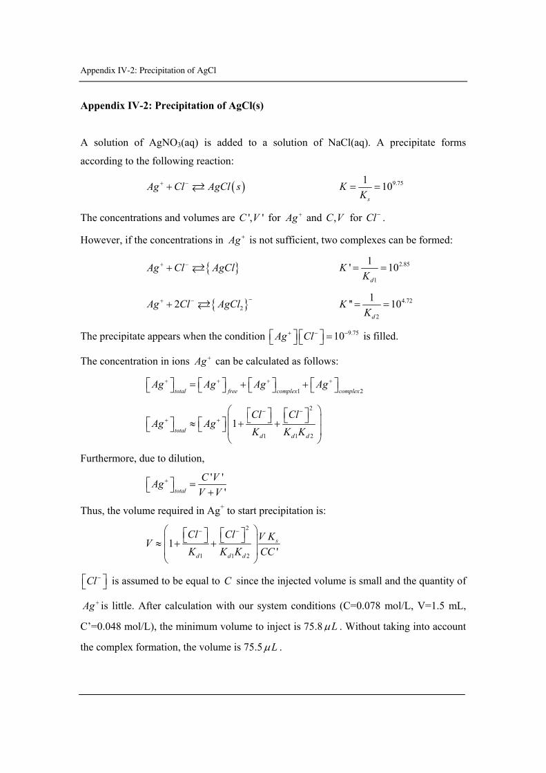
Appendix IV-2: Precipitation of AgCl
Appendix IV-2: Precipitation of AgCl(s)
A solution of AgNO3(aq) is added to a solution of NaCl(aq). A precipitate forms
according to the following reaction:
( )Ag Cl AgCl s+ −+ 9.751 10s
KK
= =
The concentrations and volumes are ', 'C V for Ag + and ,C V for Cl− .
However, if the concentrations in Ag + is not sufficient, two complexes can be formed:
{ }Ag Cl AgCl+ −+ 2.85
1
1' 10d
KK
= =
{ }22Ag Cl AgCl −+ −+ 4.72
2
1'' 10d
KK
= =
The precipitate appears when the condition 9.7510Ag Cl+ − −⎡ ⎤ ⎡ ⎤ =⎣ ⎦ ⎣ ⎦ is filled.
The concentration in ions Ag + can be calculated as follows:
1 2total free complex complexAg Ag Ag Ag+ + + +⎡ ⎤ ⎡ ⎤ ⎡ ⎤ ⎡ ⎤= + +⎣ ⎦ ⎣ ⎦ ⎣ ⎦ ⎣ ⎦
2
1 1 2
1total
d d d
Cl ClAg Ag
K K K
− −+ +
⎛ ⎞⎡ ⎤ ⎡ ⎤⎣ ⎦ ⎣ ⎦⎜ ⎟⎡ ⎤ ⎡ ⎤≈ + +⎣ ⎦ ⎣ ⎦ ⎜ ⎟⎝ ⎠
Furthermore, due to dilution,
' ''total
C VAgV V
+⎡ ⎤ =⎣ ⎦ +
Thus, the volume required in Ag+ to start precipitation is: 2
1 1 2
1's
d d d
Cl Cl V KVK K K CC
− −⎛ ⎞⎡ ⎤ ⎡ ⎤⎣ ⎦ ⎣ ⎦⎜ ⎟≈ + +⎜ ⎟⎝ ⎠
Cl−⎡ ⎤⎣ ⎦ is assumed to be equal to C since the injected volume is small and the quantity of
Ag + is little. After calculation with our system conditions (C=0.078 mol/L, V=1.5 mL,
C’=0.048 mol/L), the minimum volume to inject is 75.8 Lμ . Without taking into account
the complex formation, the volume is 75.5 Lμ .
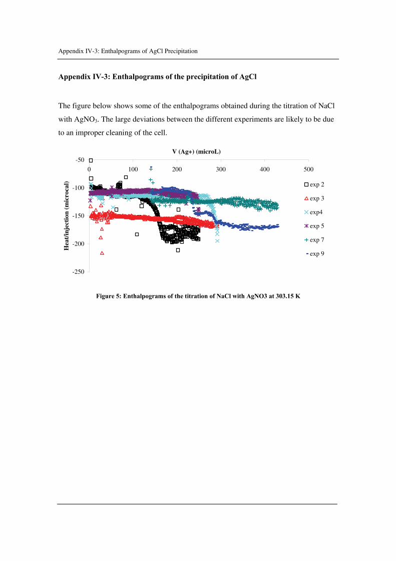
Appendix IV-3: Enthalpograms of AgCl Precipitation
Appendix IV-3: Enthalpograms of the precipitation of AgCl
The figure below shows some of the enthalpograms obtained during the titration of NaCl
with AgNO3. The large deviations between the different experiments are likely to be due
to an improper cleaning of the cell.
-250
-200
-150
-100
-50
0 100 200 300 400 500
V (Ag+) (microL)
Hea
t/in
ject
ion
(mic
roca
l) exp 2
exp 3
exp4
exp 5
exp 7
exp 9
Figure 5: Enthalpograms of the titration of NaCl with AgNO3 at 303.15 K
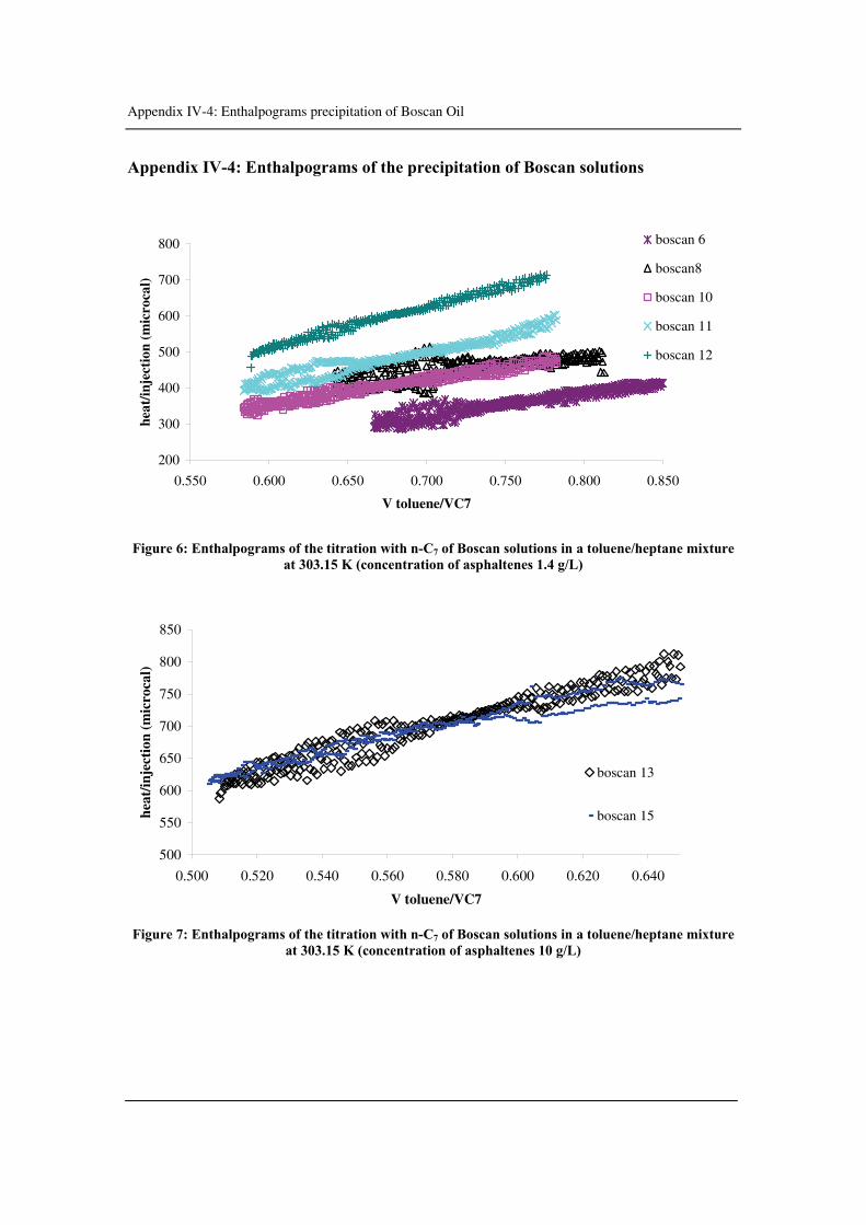
Appendix IV-4: Enthalpograms precipitation of Boscan Oil
Appendix IV-4: Enthalpograms of the precipitation of Boscan solutions
200
300
400
500
600
700
800
0.550 0.600 0.650 0.700 0.750 0.800 0.850
V toluene/VC7
heat
/inje
ctio
n (m
icro
cal)
boscan 6
boscan8
boscan 10
boscan 11
boscan 12
Figure 6: Enthalpograms of the titration with n-C7 of Boscan solutions in a toluene/heptane mixture at 303.15 K (concentration of asphaltenes 1.4 g/L)
500
550
600
650
700
750
800
850
0.500 0.520 0.540 0.560 0.580 0.600 0.620 0.640
V toluene/VC7
heat
/inje
ctio
n (m
icro
cal)
boscan 13
boscan 15
Figure 7: Enthalpograms of the titration with n-C7 of Boscan solutions in a toluene/heptane mixture
at 303.15 K (concentration of asphaltenes 10 g/L)