Experimental Study of Free Convection Inside Curvy

Engineering Science 2017; 2(4): 85-92

http://www.sciencepublishinggroup.com/j/es

doi: 10.11648/j.es.20170204.11

Experimental Study of Free Convection Inside Curvy Surfaces Porous Cavity

Ali Maseer Gati'a, Zena Khalifa Kadhim, Ahmad Kadhim Al-Shara

Mechanical Department, Engineering College, Wasitt University, Wasit, Iraq

Email address:

[email protected] (A. M. Gati'a), [email protected] (Z. K. Kadhim), [email protected] (A. K. Al-Shara)

To cite this article: Ali Maseer Gati'a, Zena Khalifa Kadhim, Ahmad Kadhim Al-Shara. Experimental Study of Free Convection Inside Curvy Surfaces Porous

Cavity. Engineering Science. Vol. 2, No. 4, 2017, pp. 85-92. doi: 10.11648/j.es.20170204.11

Received: April 17, 2017; Accepted: April 27, 2017; Published: August 1, 2017

Abstract: An experimental investigation is performed in the present study to identify how can the porous medium behave

inside a closed curvy porous cavity heated from below and compare the obtained results with the same numerical simulation

model. The numerical model is simulated by ANSYS-CFX R15.0 under Darcy-Forchheimer model with neglecting the viscous

dissipation. The work contains also measuring experimentally the permeability of the sand-silica which represents the solid

matrix of the porous medium by using a special device made locally. The isotherms form and the temperature distribution on

the interior sides of the walls are what explored in this experimental work. The final result leads to an acceptable convergence

between these two models (numerical and experimental models). Also, the work gives a proof of the legality of Kozeny-

Karman equation to estimate the permeability of the porous medium mathematically.

Keywords: Free Convection, Curvy Cavity, Porous Medium, Sand-Silica, Teflon, Darcy-Forchheimer Model

1. Introduction

This research is an integral part of our previous study

which was published recently under the title (Numerical

Study of Laminar Free Convection Heat Transfer Inside a

Curvy Porous Cavity Heated From Below) [1]. In order to

complete the main purpose of this numerical study about

the effect of the PM on the convection HT inside a closed

wavy cavity, we turned to the practical side via the use of

two devices have been made locally here in this

experimental work. One of them is designed according to

the Heinemann's schema [2] which will be shown later to

measure the permeability of the used PM (saturated silica-

sand by water), whereas the other is designed to simulate

only one numerical model practically. To identify the

isotherms form it was used the Thermal Imager (thermal

camera), while the thermocouples (K-type) were used to

estimate the temperature distribution.

Silica is the name given to a group of minerals

composed of silicon and oxygen, the two most abundant

elements in the earth's crust. Silica is found commonly in

the crystalline state and rarely in an amorphous state. It is

composed of one atom of silicon and two atoms of oxygen

resulting in the chemical formula (SiO2). Sand consists of

small grains or particles of mineral and rock fragments.

Although these grains may be of any mineral composition,

the dominant component of sand is the mineral quartz,

which is composed of silica (silicon dioxide). Other

components may include aluminum, feldspar and iron-

bearing minerals. Sand with particularly high silica levels

that is used for purposes other than construction is

referred to as silica sand or industrial sand [3].

2. Numerical Chosen Model

The chosen numerical model is a two dimensional closed

cavity filled with a PM. The side facing walls are sketched to

be wavy sinusoidal walls. One of them (right one) is reflected

about the vertical center line of the cavity as displayed in

Figure 1. Number of waves per wall (N) is equal to (1) with

wave's amplitude (ad) equal to (0.15). As a boundary

conditions, the facing side walls of the model are kept

insulated to be adiabatic walls. The top surface is exposed to

outside environment while the bottom surface is exposed to

constant heat flux.

86 Ali Maseer Gati'a et al.: Heat Transfer by Convection in a Curved Porous Cavity a Design of the Experimental Model

Figure 1. Numerical chosen model and boundary conditions.

3. Experimental Devices

As mentioned above, there are two main devices, one of

them is used to measure the permeability of the chosen sand-

silica and the other is used to simulate practically one

selected numerical model only. Each one of them will be

explained briefly in the following topics.

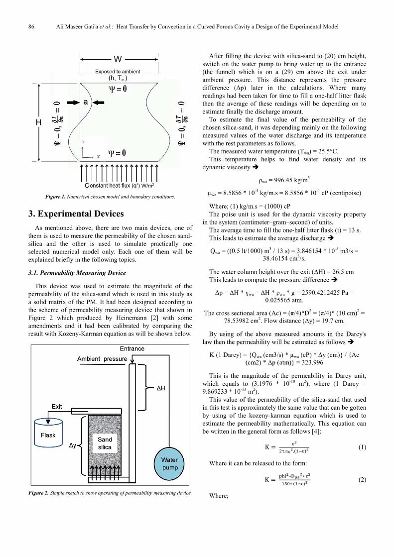
3.1. Permeability Measuring Device

This device was used to estimate the magnitude of the

permeability of the silica-sand which is used in this study as

a solid matrix of the PM. It had been designed according to

the scheme of permeability measuring device that shown in

Figure 2 which produced by Heinemann [2] with some

amendments and it had been calibrated by comparing the

result with Kozeny-Karman equation as will be shown below.

Figure 2. Simple sketch to show operating of permeability measuring device.

After filling the devise with silica-sand to (20) cm height,

switch on the water pump to bring water up to the entrance

(the funnel) which is on a (29) cm above the exit under

ambient pressure. This distance represents the pressure

difference (∆p) later in the calculations. Where many

readings had been taken for time to fill a one-half litter flask

then the average of these readings will be depending on to

estimate finally the discharge amount.

To estimate the final value of the permeability of the

chosen silica-sand, it was depending mainly on the following

measured values of the water discharge and its temperature

with the rest parameters as follows.

The measured water temperature (Twa) = 25.5°C.

This temperature helps to find water density and its

dynamic viscosity �

ρwa = 996.45 kg/m3

µwa = 8.5856 * 10-4

kg/m.s = 8.5856 * 10-1

cP (centipoise)

Where; (1) kg/m.s = (1000) cP

The poise unit is used for the dynamic viscosity property

in the system (centimeter–gram–second) of units.

The average time to fill the one-half litter flask (t) = 13 s.

This leads to estimate the average discharge �

Qwa = ((0.5 lt/1000) m3 / 13 s) = 3.846154 * 10

-5 m3/s =

38.46154 cm3/s.

The water column height over the exit (∆H) = 26.5 cm

This leads to compute the pressure difference �

∆p = ∆H * ɣwa = ∆H * ρwa * g = 2590.4212425 Pa =

0.025565 atm.

The cross sectional area (Ac) = (π/4)*D2 = (π/4)* (10 cm)

2 =

78.53982 cm2. Flow distance (∆y) = 19.7 cm.

By using of the above measured amounts in the Darcy's

law then the permeability will be estimated as follows �

K (1 Darcy) = {Qwa (cm3/s) * µwa (cP) * ∆y (cm)} / {Ac

(cm2) * ∆p (atm)} = 323.996

This is the magnitude of the permeability in Darcy unit,

which equals to (3.1976 * 10-10

m2), where (1 Darcy =

9.869233 * 10-13

m2).

This value of the permeability of the silica-sand that used

in this test is approximately the same value that can be gotten

by using of the kozeny-karman equation which is used to

estimate the permeability mathematically. This equation can

be written in the general form as follows [4]:

K � ��

��.�.� ��

(1)

Where it can be released to the form:

K � ��

��

�� (2)

Where;

Engineering Science 2017; 2(4): 85-92 87

av: is the specific internal surface area of the medium (ratio

of the exposed surface area to the solid volume).

τ: is the tortuosity of the medium (varies between 2 and 3).

The tortuosity is commonly used to describe the diffusion in

PM [5]. In the simplest mathematical method the tortuosity

equals to ratio of the curve length to the distance between the

ends of it [6].

Phi: is the spherisity of the beads or the shape factor

(dimensionless).

For the silica-sand used in this test, taking phi=0.65,

Dpa=0.001m, and ɛ=0.36 where the range of the spherisity of

silica-sand beads can guess its value approximately between

(0.75 – 0.65), then:

K � �.��.�� .��

�� .�� 3.20836 * 10

-10 m

2

3.2. Experimental Test Device

3.2.1. Manufacturing Steps

A numerical model has been chosen to simulate it

practically which is taken from the reflected facing wall

models as illustrated in Figure 3. It can be described by the

following characteristics, where it have a (20) cm for height,

one wave per height, (3) cm for wave wall amplitude, and

aspect ratio equal to one.

Figure 3. A sketch of experimental model (front view).

This model was simulated practically by using of a three

different materials; Aluminum plate was used for top and

bottom surfaces with (4) mm in thickness, A Teflon plate was

used for walls and back side with (27) mm in thickness, and a

transparent plastic plate (known as acrylic or acrylic glass)

was used for front side with (5) mm in thickness. The two

important properties of these last two materials are the

sufficient resistance of heating beside the easiness of

forming. The main steps to complete this work can be

explained as follows:

(1) Manufacturing the wavy walls by using of electrical

saw and finishing them by a milling machine. Then fixed

them on the back side in their right position as shown in

Figure 4 by using of a universal fast adhesive which is a set

of activator and high viscosity cyanoacrylate adhesive called

(Professional Soma Fix S663).

(2) Fixing thermocouples (K-type) in the wavy walls (three

for each wall) by inserting each one of them into a hole of (6)

mm in diameter which then is reduced to be (1-1.5) mm in

diameter before reaching the end by (5) mm distance

approximately. So that only the head of each thermocouple

appears on the wavy side surface. To prevent water from

entering these holes it was injected thermal silicone inside

them which is a high temperature resistant RTV silicone used

usually for fuel engines gasket. Figure 5 shows how this

operation was achieved.

Figure 4. Wavy walls and back side from Teflon.

Figure 5. Fixing thermocouples on wavy walls.

(3) Closing the front side of the cavity with the transparent

plastic plate by using of four bolts (5) mm in diameter on

each side after painting the touching surface by thermal

silicone to ensure perfect contact and prevent seepage of

water as shown in Figure 6.

Figure 6. Closing the front side of the cavity and filling it by PM.


(4) Fixing the top and the bottom surfaces which are

made from Aluminum plate (4) mm in thickness by using

(8) expansion bolt screw with plastic anchors (6mm) for

each one after painting touching surfaces by thermal

silicone as shown in Figure 7. The important two steps

before fixing the top surface were the adding of the

chosen silica-sand and distilled water inside the cavity

which represent the PM stuff and the fixing of

thermocouples on each one of the top and bottom surfaces.

This last step was achieved by using an adhesive epoxy

putty (ALTECO Epo Putty A + B). It consists of two

putties which are Resin (A) and Hardener (B), they are

blended together by water and then the resulting paste is

used in the place to be.

As an additional step to ensure that the porosity value

of the chosen silica-sand is measured correctly, the cavity

has been filled with water before adding the chosen silica-

sand as much as represented the amount of the porosity

from the overall size of the cavity. Where the overall size

of the cavity was measured by ANSYS-CFX program. The

result of this step was came fully confirmed the accuracy

of the porosity value which have been estimated in the

manner described in the paragraph 4.2.

A. Before fixing. B. After fixing.

Figure 7. Fixing the bottom cover and its thermocouples.

(5) Fixing the Heater under the bottom surface, where it

is a Halogen heater (400W/230V) comprises tungsten

filaments in sealed quartz envelopes, mounted in front of a

metal reflector as shown in Figure 8. It operates "at a

higher temperature than Nichrome wire heaters but not as

high as incandescent light bulbs, radiating primarily in the

infrared spectrum. It converts up to 86% of their input

power to radiant energy, losing the remainder to

conductive and convective heat" [6].

The main reason of using this type of heaters is to

ensure that the supplied heat flux will be distributed

equally on all the bottom area of the cavity, where –as

mentioned above- it converts up to 86% of their input

power to radiant energy.

Figure 8. Halogen Heater (400W/230V).

3.2.2. Description of Some Used Materials

In this work there are two important materials that have

been used, it is needed to be described here to complete this

section as follows:

(i). Transparent Plastic Plate

It is a Poly (methyl methacrylate) (PMMA), also known

as acrylic or acrylic glass as well as by the trade names

plexiglas, Acrylite, Lucite, and Perspex, is a transparent

thermoplastic often used in sheet form as a lightweight or

shatter-resistant alternative to glass. The same material

can be utilized as a casting resin, in inks and coatings, and

has many other uses [7]. Table 1 shows its general

properties.

Table 1. General properties of acrylic glass [8].

Melting point 160°C (433 K)

Thermal conductivity 0.17 - 0.2 W/(m·K)

(ii). Teflon (PTFE), Polytetrafluoroethylene

It is a synthetic fluoropolymer of tetrafluoroethylene

that has numerous applications. The best known brand

name of PTFE-based formulas is Teflon by Chemours.

Chemours is a spin-off of DuPont Company, which

discovered the compound in 1938 [9]. Table 2 shows its

general properties.

Table 2. General properties of Teflon [8].

Melting point 327°C (600°K)

Thermal conductivity 0.25 W/(m·K)

3.2.3. Operating the Device

The test device has been operated inside an air-

conditioning room to provide two important conditions; the

first is a constant ambient temperature while the second is a

stability in overall ambient HT coefficient. To get a

constant heat flux from the Heater it was supplied a

constant electrical current by using of a supply voltage

regulator. The steady state was estimated by notice that the

temperature at a two chosen points are not changed with

time, where this was realized after passing (13) hours

approximately as illustrated in Figure 9 below.


Each (θ) represents temperature in different place.

Figure 9. Time for steady state (θ = reading temp./ final temp.).

It is important to know the way of estimating the value of

the overall ambient HT coefficient (ha or OAHTC), where

this done by three steps as follows �

(1) Calculating heat losses: there are -in general- three

important directions needed to find the heat transfer losses from

them. These directions are (front, back, and the sides), where:

qsi = the sides heat losses (W/m2).

qfr = the front heat losses (W/m2).

qba = the back heat losses (W/m2).

All of them can be calculated by using of the simple

conduction heat transfer equation (Fourier equation). For

example; a case that have (qin = 2238 W/m2) the losses can

be calculating as below:

qsi = - ∆Tsi / [∑dx/∑k]

= - ∆Tsi [(1 / [(2*(∑dx/3) / kteflon) + (2*dxglasswool/ kglasswool)])

= - 16.5 [(1 / [(0.12/ 0.25) + (0.01/ 0.04))

= - 22.6 W/m2

Where; (∆Tsi = Average interior side temperature – Ta) and

∑dx is the summation of the distance between inside points

(thermocouples points) and the outside (∑dx= 0.09 + 0.06 +

0.03=0.18) as illustrated in Figure 10.

Figure 10. Position of dx1, dx2, and dx3.

qba = - ∆Tba / [∑dx/∑k]

= ∆Tba [(1 / [(dx4/ kteflon) + (dxglasswool/ kglasswool)])

= 16.5 [(1 / [(0.027/ 0.25) + (0.005/ 0.04)])

= - 70.8 W/m2

Where; dx4 is the back side thickness (made from Teflon).

qfr = - ∆Tfr / [∑dx/∑k]

= ∆Tfr [(1 / [(dxacrylicglass/ kacrylicglass) + (dxglasswool/ kglasswool)])

= 16.5 [(1 / [(0.005/ 0.17) + (0.005/ 0.04)])

= - 107 W/m2

Then;

qtolosses = Total heat losses

= qsi + qba + qfr = 22.6 + 70.8 + 107 = 200.4 W/m2

This means the percentage heat losses is (9%)

approximately from the total supplied heat flux.

(2) Calculating the out heat transfer (qout):

qin = qout + qtolosses

2238 = qout + 200.4

qout = 2037.6 W/m2

(3). Calculating the overall ambient heat transfer coefficient:

qout = ha. ∆Ttop

2037.6 = ha * 6 � ha = 339.6 W/m2. K (this large amount

is due to the forced convection on the top surface of the

device beside containing the other dissipation factors of heat

like radiation).

Where; ∆Ttop = Ttop – Ta

The procedure to operate the test device includes the

following main steps:

(1) Setting up the device in an air-conditioning room

nearing from a ceiling fan. This fan provided a speed of air

vacillated between 0.33 to 3 m/s which measured by the

Anemometer near the upper surface of the model.

(2). Balancing its situation with respect to the ground

where y-axis of the device should be in a perpendicular

direction to the ground.

(3). Supplying the specified electric power by the Slide

Regulator to the Heater. Where the amount of both the

supplied voltage and the electrical current were measured by

the Ammeter.

(4). Recording the temperature for each specified points at

every period of time. Each period was about 15 to 30 minutes

until reaches the steady state where the temperature did not

change with time. Also it was recorded the ambient

temperature and the speed of air near the upper surface by

using of the Hot Wire device. To estimate the heat losses, it

was reading the temperature on the sides of devices which

are defined above.

4. Results

4.1. Isotherm Lines

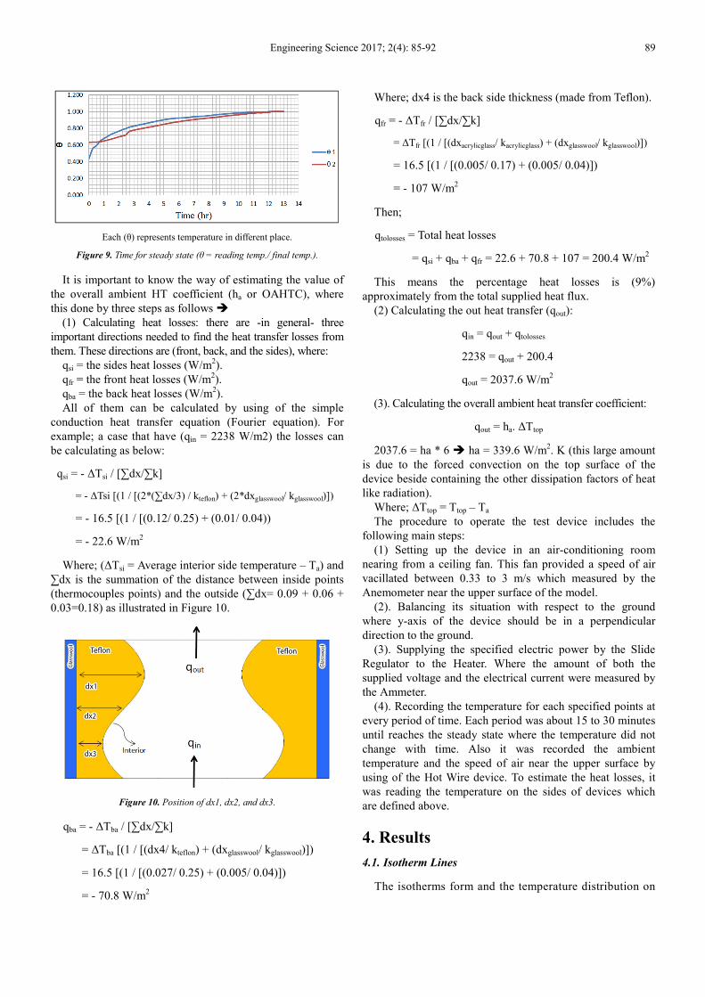
The isotherms form and the temperature distribution on


the interior side of the walls are what explored in this

experimental work. To estimate the isotherms form it was

used the Thermal Imager by focusing its lens towards the

transparent side of the practical model when reaching the

steady state then take a picture (thermal image). figures

(11, 12, and 13) compare between the practical isotherms

form and the theoretical one for the chosen model. As a

result it can be said that there is a sketchy match between

the two images.

Figure 11. The transparent side of the practical model.

Figure 12. Theoretical isotherms (state3).

Figure 13. Practical isotherms.

4.2. Temperature Distribution

On the other hand, the temperature distribution on the

interior sides of the cavity's walls is obtained by using a

collection of thermocouples which were distributed on these

sides as explained in Chapter Four. These eleven

thermocouples were distributed as: three on each facing

walls, three on the base, and two on the roof of the cavity and

three amount of heat flux were supplied. Table 3 shows a

comparison between experimental and corresponding

theoretical results.

Table 3. Experimental and theoretical results.

Details State 1 State 2 State 3

Ie=0.57 Amber. Ie=0.54 Amber Ie=0.42 Amber.

Ve=21.2 Volt. Ve=16.9 Volt Ve=10 Volt.

Pe=12.084 Watt

(2238 W/m2).

Pe=9.126 Watt

(1538 W/m2).

Pe=4.2 Watt (778

W/m2).

1. Results:

Dimensionless temperature distribution

Points θex θth θex θth θex θth

1 0.668 0.798 0.721 0.822 0.820 0.879

2 0.630 0.794 0.685 0.818 0.811 0.874

3 0.585 0.768 0.649 0.794 0.786 0.852

4 0.665 0.798 0.721 0.822 0.822 0.878

5 0.622 0.794 0.685 0.818 0.814 0.874

6 0.585 0.767 0.649 0.793 0.786 0.852

7 0.993 0.916 0.997 0.925 0.994 0.947

8 1.000 1.000 1.000 1.000 1.000 1.000

9 0.975 0.917 0.985 0.926 0.989 0.947

10 0.482 0.714 0.555 0.752 0.680 0.829

11 0.479 0.714 0.551 0.751 0.682 0.828

θ = reading temperature /maximum reading temperature

θth = theoretical dimensionless temperature distribution.

θex = experimental dimensionless temperature distribution.

2. GNN

35.8 33.8 35.4 30.5 28.7 22.1

2. Ra

1157 1219 802 847 419 449

Figure 14 below shows the position of each point.

Figure 14. Shows the position of each point.

To complete the above comparison that shown in the

previous table there are some important points which can be

indicated as follows:

(1) To compute GNN for the practical model it is


depending on the obtainable temperatures, where the bulk

temperature is estimated to be equal to [(Tp1 + Tp2 + Tp3 +

Tp4 + Tp5 + Tp6 + Tp10 + Tp11)/8]. While the base

temperature is taken to be equal to [(Tp7 + Tp8 + Tp9)/3].

(2) The experimental GNN is calculated with the available

values. Where the bulk temperature is taken as the average

value for the points (1, 2, 3, 4, 5, 6, 10, and 11), while the

base temperature is taken as the average value for the points

(7, 8, and 9).

(3) The temperature distribution for the side walls is

graduated in descending from the lower point to the upper

one for both the theoretical and the experimental ratios.

(4) For both distributions the maximum temperature value

occurs in the middle of the base (P8).

(5) The mean percentage error in the temperature

distribution of the experimental values with respect to the

theoretical values is (14%) for all three states. This done by

using of the standard percentage error formula which takes

here the form (percentage error = [(θth-θex)/θth]*100) and then

it is taken the average as a mean (total) percentage error for

all variables and all states.

(6) The mean percentage error for the GNN of the

experimental values with respect to the theoretical values is

(17.3%) for all three states.

(7) The points where the gap is greatest between the practical

and theoretical results are (10 and 11) at the upper surface.

4.3. Mismatch Reasons

The mismatch between the experimental and theoretical

results can be traced back to the following reasons:

(1) Losses in the supplied heat flux due to non-perfectly

insulation.

(2) Roughness of the inside curvy walls.

(3) Instability of electricity beside the long time needed to

reach the steady state.

(4) HT through walls by conduction from the base, which

it was tried to prevent it by using of a material have a

small value of thermal conductivity (Teflon and acrylic

glass).

(5) Non-perfectly purity of used water.

(6) Errors in measurement devices.

(7) Missing of exactly properties of used materials.

(8) Blemishes in the solid matrix.

5. Conclusions

There is an important match between the numerical

isotherm form and corresponding experimental isotherm

form. This match gives additional strength to the legitimacy

of the numerical research and the validity of the results

obtained. Beside the match also of the temperature

distribution on the interior side of the cavity walls.

The importance of this match comes as it proves the

validity of the theoretical equations that used in the

numerical simulation under Darcy-Forchheimer model.

The experimental results for heat transfer behavior inside

the wavy closed porous cavity shows that the percentage

approach with the corresponding numerical results is closed

to be (85%) approximately. Also it is important to show that

the permeability measuring device that designed and

manufactured in the present work measures the permeability

for the used silica-sand with percentage error equals to

(0.34%) with respect to the kozeny-karman equation which

measures the permeability mathematically.

Nomenclature

Symbol Description Symbol Description

Ra Modified Rayleigh number. g Gravitational acceleration (m/s2).

Nu Nusselt number. A Aspect ratio.

T Temperature. N Number of waves per height.

k Thermal conductivity (W/m. K). a Wave's amplitude (m).

K Permeability (m2). ad Dimensionless wave's amplitude (a/H).

u Velocity component at x-axis (m/s). α Thermal diffusivity (m2/s).

ν Velocity component at y-axis (m/s). X Stream function.

W Cavity width (m). q0 (HF) Heat flux (W/m2).

H Cavity height (m).

Subscript Description Subscript Description

eff Effective. f Fluid.

s Solid. a Ambient.

Acronym

Description

PM

PM (media or medium).

HT

Heat transfer.

GNN

Global Nusselt number.

OAHTC

Overall ambient heat transfer coefficient (W/m2. K).


References

[1] Ali Maseer Gati'a, Zena Khalifa Kadhim, and Ahmad Kadhim Al-Shara.'Numerical Study of Laminar Free Convection HT Inside a Curvy Porous Cavity Heated From Below'. Engineering Science journals. Vol. 2, Issue 2, April 2017.

[2] Zoltan E. HEINEMANN. 'Fluid Flow in Porous Media'. Textbook series, Volume 1, DI Barbara Schatz, October 2005.

[3] EUROSOIL, which is a member of IMA-Europe, the European Industrial Minerals Association, was founded in May 1991 as the official body representing the European industrial silica producers.

[4] Manmath N. Panda, and Larry W. Lake. 'Estimation of single-phase permeability from parameters of particle-size distribution'. AAPG Bull 1994; 78: 1028–39.

[5] Epstein, N. (1989), On tortuosity and the tortuosity factor in flow and diffusion through porous media, Chem. Eng. Sci., 44(3), 777– 779.

[6] ASHRAE Handbook - Heating, Ventilating, and Air-Conditioning Systems and Equipment (I-P Edition) American Society of Heating, Refrigerating and Air-Conditioning Engineers, Inc., 2008, Electronic ISBN 978-1-60119-795-5, table 2 page 15. 3.

[7] Hydrosight. "Acrylic vs. Polycarbonate: A quantitative and qualitative comparison" (http://www.hydrosight.com/acrylic-vs-polycarbonate-a-quantitative-and-qualitative-comparison).

[8] The free encyclopedia Wikipedia.

[9] Teflon™| Chemours Teflon™ Nonstick Coatings and Additives. www.chemours.com. Retrieved 2016-03-01. (https://www.chemours.com/Teflon/en_US)

[10] George S. Kell. 'Density, thermal expansivity, and compressibility of liquid water from 0 to 150 C: correlations and tables for atmospheric pressure and saturated reviewed and expressed on 1968 temperature scale'. journal of chemical and engineering data, Vol. 20, No. 1, 1975.

Documents

Experimental Study of Free Convection Inside Curvy