Experimental Study of Heat Transfer Coefficient and Film

Master of Science Thesis

KTH School of Industrial Engineering and Management

TRITA-ITM-EX 2019:120

Division of Energy Technology EGI

SE-100 44 STOCKHOLM

Experimental Study of Heat Transfer

Coefficient and Film Cooling Effectiveness

Ke Li

I

Master of Science Thesis: TRITA-ITM-EX 2019:120

Experimental Study of Heat Transfer Coefficient and

Film Cooling Effectiveness

Ke Li

Approved

2019-04-04

Examiner

Paul Petrie-Repar

Supervisor

Jens Fridh

Commissioner

Siemens Industrial Turbimachinery AB

Contact person

Mats Kinell

ABSTRACT

This thesis investigates the possibility to evaluate the film cooling thermal performance on flat

plate using Thermochromic Liquid Crystal. After an introduction of the basic concept and

background of gas turbine blades film cooling and Thermochromic Liquid Crystal, a thorough

explanation of four methods is presented. Dimensional or similarity analysis is implemented to

build relationship between real engine and laboratory model. Also, the Reynolds number and

Blowing ratio are the fundamental of test object design and TLC selection. This study illustrated

the layout of the test rig and corresponding setups, and the following part explains the data

collection system and image processing MATLAB script which is vital for the success of data

extraction. The least square method is applied to figure time-series optimal solution in solver.

All the experiments are conducted at near room temperature as opposed to the extremely high

gas turbine exhausted gas, including two calibration test and one heat transfer experiment. The

heat transfer coefficient and film cooling effectiveness are the target objective through the entire

project. By comparison with a similar experiment in a literature, the outcomes partially validated

the film cooling performance under the pre-set flow and thermal condition and the Liquid

Crystal thermography technique is proved to be a trustworthy method to mapping heat transfer

surface.

II

Examensarbete: TRITA-ITM-EX 2019:120

Experimental Study of Heat Transfer Coefficient and

Film Cooling Effectiveness

Ke Li

Godkänt

2019-04-04

Examinator

Paul Petrie-Repar

Handledare

Jens Fridh

Uppdragsgivare

Siemens Industrial Turbimachinery AB

Kontaktperson

Mats Kinell

SAMMANFATTNING

Denna avhandling undersöker möjligheten att utvärdera filmkylningens termiska prestanda på

plan platta med användning av Termokromisk Flytande Kristall (TLC). Efter en introduktion av

grundkonceptet och bakgrunden till gasturbinbladens filmkylning och termokromisk flytande

kristall presenteras en grundlig förklaring av fyra metoder. Dimensionell eller likhetsanalys

implementeras för att bygga upp förhållandet mellan verklig motor och laboratoriemodell.

Reynoldstalet och blåsningsförhållandet (blowing ratio) är också grunden för testobjektdesign

och TLC-val. Denna studie illustrerade provriggens layout och tillhörande inställningar. I

följande del förklaras datainsamlingssystemet och bildbehandling, MATLABTM-skriptet som är

avgörande för framgång med datautvärdering. Den minsta kvadratiska metoden tillämpas för att

hitta tidsseriens optimala lösning i lösaren.

Alla experiment utförs vid nära rumstemperatur i motsats till den höga temperature på

gasturbingasen, inklusive två kalibreringstest och ett värmeöverföringsexperiment.

Värmeöverföringskoefficienten och filmkylningseffektiviteten är målmålet genom hela projektet.

Resultaten validerade partiellt filmkylningens prestanda under det förinställda flödet och det

termiska tillståndet. Liquid Crystal-termografitekniken har visat sig vara en pålitlig metod för att

kartlägga värmeöverföringsytan jämfört med ett liknande experiment i den öppna litteraturen.

III

TABLE OF CONTENTS

ABSTRACT ............................................................................................................. I

SAMMANFATTNING .......................................................................................... II

TABLE OF CONTENTS ..................................................................................... III

LIST OF FIGURES ............................................................................................... V

LIST OF TABLES .............................................................................................. VII

FOREWORD ..................................................................................................... VIII

NOMENCLATURE ............................................................................................. IX

1 INTRODUCTION .......................................................................................... 1

1.1 Background and Motivation ................................................................. 1

1.2 Objectives ............................................................................................... 4

2 METHODOLOGIES ...................................................................................... 5

2.1 Transient heat Transfer Experiment ................................................... 5

2.1.1 Method 1 ....................................................................................... 7

2.1.2 Method 2 ....................................................................................... 8

2.1.3 Method 3 ....................................................................................... 8

2.1.4 Method 4 ..................................................................................... 10

2.2 Dimensional Analysis .......................................................................... 10

2.2.1 Hole Geometry Based Distance (x/D, y/D) .............................. 10

2.2.2 Blowing Ratio (M) ..................................................................... 11

2.2.3 Reynold Number (Re) ............................................................... 11

2.3 Thermochromic Liquid Crystal ......................................................... 12

2.3.1 Thermochromic Liquid Crystal .............................................. 12

2.3.2 RGB Theory .............................................................................. 14

2.3.3 HSV Theory ............................................................................... 16

2.3.4 Hue-Temperature Distance Weight ........................................ 17

IV

3 EXPERIMENT PROCESS ............................................................................ 19

3.1 Pre-setup ............................................................................................... 19

3.1.1 Test rig ........................................................................................ 19

3.1.2 Test object ................................................................................... 20

3.1.3 Measurement equipment ........................................................... 23

3.2 Experiment ........................................................................................... 23

3.2.1 Thermocouple Calibration ........................................................ 23

3.2.2 Thermochromic Liquid Crystal Calibration ........................... 25

3.2.3 Heat Transfer Experiment ........................................................ 25

3.3 Post-process .......................................................................................... 26

3.3.1 Data collection and transformation .......................................... 27

3.3.2 Denoising ..................................................................................... 27

3.3.3 Solver ........................................................................................... 28

4 RESULTS AND DISCUSSION ................................................................... 31

4.1 Calibration ........................................................................................... 31

4.2 Transient Heat Transfer Experiment ................................................ 33

5 UNCERTAINTY AND CONCLUSIONS .................................................. 37

5.1 Uncertainty ........................................................................................... 37

5.2 Conclusions........................................................................................... 39

6 FUTURE WORK .......................................................................................... 41

REFERENCES ..................................................................................................... 44

APPENDIX A: EQUATION DERIVATION ..................................................... 46

APPENDIX B: DIMENSIONAL ANALYSIS ................................................... 50

APPENDIX C: PROTOCOLS ............................................................................ 51

V

LIST OF FIGURES

Figure 1 The Development Turbine Cooling (Hah, 1997) .............................................................. 1

Figure 2 Schematic of Film Cooling Configurations on A Vane (Bogard, n.d.) ............................ 2

Figure 3 Duhamel Superposition Principle (Huang, 1998) ............................................................. 9

Figure 4 Surface Coordinate ......................................................................................................... 11

Figure 5 Liquid Crystals Classification (Hallcrest, n.d.)............................................................... 12

Figure 6 TLC Phase Changes with Temperature Changing (Hallcrest, u.d.)................................ 13

Figure 7 Temperature-sensitive TLC Color Spectrum (Hallcrest, n.d.) ........................................ 14

Figure 8 Temperature-insensitive TLC Color Spectrum (Hallcrest, n.d.) .................................... 14

Figure 9 Bayer Filter (Wikipedia, 2018) ....................................................................................... 15

Figure 10 Bayer Filter Principle (Wikipedia, 2018) ..................................................................... 15

Figure 11 HSV Cylinder (Wikipedia, 2019) ................................................................................. 16

Figure 12 HSV Cone (Marques, 2011) ......................................................................................... 17

Figure 13 TLC Distance Weight Method ...................................................................................... 18

Figure 14 Test Rig Layout ............................................................................................................ 20

Figure 15 Sectional View of Test Chamber and Flow Direction .................................................. 20

Figure 16 Test Surface with Applied TLC .................................................................................... 21

Figure 17 Thermocouple Arrangement ......................................................................................... 22

Figure 18 Lateral View of Test Surface ........................................................................................ 22

Figure 19 NetScanner and DATASCAN ...................................................................................... 23

Figure 20 TC calibration Set-up .................................................................................................... 24

Figure 21 Thermocouple Calibration ............................................................................................ 24

Figure 22 Temperature and Hue Correlation ................................................................................ 25

Figure 23 Transient Test Object .................................................................................................... 26

Figure 24 Workflow of Transferring from RAW to MAT........................................................... 27

Figure 25 Hue Denoising Process ................................................................................................. 28

Figure 26 Local Driving Temperature Calculation ....................................................................... 29

Figure 27 Solver Workflow for One Pixel .................................................................................... 29

VI

Figure 28 HTC and Film Cooling Effectiveness Map .................................................................. 33

Figure 29 Span Wise Average ....................................................................................................... 34

Figure 30 Residual of Exhaustion Method .................................................................................... 34

Figure 31 Hue for One Pixel ......................................................................................................... 35

Figure 32 Improved Span Wise Average ...................................................................................... 36

Figure 33 Schema of Experiment Apparatus (Toriyama, 2016) ................................................... 41

Figure 34 Illumination Influence................................................................................................... 42

Figure 35 Boundary Influence....................................................................................................... 43

Figure 36 Type K Thermocouple Calibration Protocol ................................................................ 51

Figure 37 Pt-100 Calibration Protocol .......................................................................................... 53

Figure 38 Temperature Indicator Calibration Protocol ................................................................. 54

VII

LIST OF TABLES

Table 1 Thermocouple Calibrated Coefficients ............................................................................ 31

Table 2 Thermochromic Liquid Crystal Calibrated Coefficients.................................................. 32

Table 3 Random Errors ................................................................................................................. 37

Table 4 Systematic Errors ............................................................................................................. 37

Table 5 Standard Uncertainty ........................................................................................................ 38

Table 6 Uncertainty of h and ..................................................................................................... 39

VIII

FOREWORD

Upon the completion of this Master Thesis, I am really grateful to those who have given me

invaluable encouragement and support during last year. First, the profound gratitude should go to

my three supervisors: Dr.Mats Kinell, Sara Rabel Carrera and Dr.Jens Fridh. They guide me

patiently through the entire process and constantly remind me of the correct research direction.

The time and energy they put on me is the embodiment of their noble personality. What is more,

I would like to present my thanks to my colleagues at SIEMEN. They have helped me a lot while

implementing experiment and analysis. Finally, I would like to extend my deep gratefulness to

my family who taught me that every detail is the factor that determines success or failure.

Thanks everything I met last year. After meet a problem that already costing you a lot of time, do

not give up at this moment. Once given up, all the previous efforts are wasted. Every step

deserves to be treated seriously, and do not deceive yourself. It's better to stop when you make a

mistake than to restart the whole process while you have been wrong for a long time. Don't

deceive yourself for the sake of a moment's comfort. In the end, you will take the price. Admit

your ignorance and incompetence. Knowing yourself correctly is the cornerstone of progress.

Ke Li

Stockholm, March 2019

IX

NOMENCLATURE

Notations

Roman Symbol Description

a error

B Sutherland’s constant for the gaseous material

Cp specific heat capacity [J/kgK]

D hole diameter [m]

h heat transfer coefficient [W/m2K]

H hue [-]

i enumerator [-]

M blowing ratio [-]

Re Reynolds number

S Saturation

t time [s]

T Temperature [K]

u standard uncertainty

v velocity [m/s]

V value [-]

x coordinate [m]

y coordinate [m]

z coordinate [m]

Greek Symbol Description

thermal diffusivity [-]

dimensionless parameter [-]

X

thickness [m]

film cooling effectiveness [-]

heat conductivity [W/mK]

viscosity [Pas]

density [g/m3]

dimensionless temperature [-]

time [s]

Subscript Description

c coolant

f film

i initial

m mainstream

r reference

w wall

aw adiabatic wall

Abbreviations

TLC Thermochromic Liquid Crystal

HTC Heat Transfer Coefficient

11

1

1 INTRODUCTION

1.1 Background and Motivation

Gas turbine engine, also called combustion turbine, is a type of heat engine, mainly composed of

compressor, combustion chamber and turbine. After the fresh air enters the gas turbine from the

intake port, it is pressurized first by the compressor into a high-pressure gas. Then, the fuel is

injected from the injector and mixed with the air. And the mixture is burned in the combustion

chamber into high-temperature and high-pressure gas. After the heating process, the high-

temperature and high-pressure gas enters the turbine section and impacts the turbine blades. The

energy is converted into a mechanical energy output, and the last exhaust gas is discharged from

the exhaust pipe.

In gas turbines engines, some components might experience extremely high temperatures up to

2000K where no suitable material could undertake such high temperature and load. To protect

the engine and extend its life span, lots of efforts are made, especially in the heat transfer aspect.

Thermal control systems and enhance cooling technologies are methods to solve heat transfer

problems. For this reason, a large amount of researches about gas turbine engines focus on the

heat transfer coefficient between hot fluid and manufactured components.

Figure 1 The Development Turbine Cooling (Hah, 1997)

As illustrated in Figure 1, with the development of cooling technologies, the turbine entry

temperature keeps increasing and meanwhile the energy transfer efficient has some improvement.

2

In the very beginning, the concept is to cool down the gas turbine blades by internal cooling flow,

where the blades are manufactured with saved air channel. While the engine runs, cold air or

other fluid coolant flows inside the channels and absorbs heat by convection. In the last 20 years,

film cooling gradually walks into the engine researches’ sight and becomes a promising topic

(Bunker, 2005).

Film cooling is a crucial step for the overall cooling of gas turbine airfoil. The holes allocated in

the blades allow coolant to inject out from the internal cavity and form a thin gaseous cooling

film right above the external surface along the mainstream-wise direction. The coolant

temperature is far lower than the exhausted gas temperature, which suppresses the heat transfer

between the mainstream and blade surface.

Figure 2 Schematic of Film Cooling Configurations on A Vane (Bogard, n.d.)

During the research stage, it is not a wise choice to implement experiment directly on real size

object, which makes similarity analysis important in order to reduce the expense. Not only

because it is costly, it is also dangerous to set an experiment under such high pressure and high

temperature. Besides, the tiny coolant holes limited the measurement of various parameters.

Eckert et al. (Eckert, 1992) investigated the possibility of estimating the thermal performance of

film cooling using geometrically similar situation. Equations and boundary conditions are made

dimensionless and the superposition is used. Vedula and Metzger (Vedula, 1991) explained an

experimental method to simultaneously obtain the local heat transfer coefficient and local film

cooling effectiveness. Their tests were conducted on a flat plate surface where two flows with

different temperatures interacted and mixed with each other. Goldstein and Taylor investigated

the heat transfer coefficient around a row of injection holes in various Blowing ratio condition

3

(Goldstein, 1982) and concluded that the high blowing ratios partially improved the reattachment

of coolant.

When the basic model of the film cooling heat transfer experiment is fixed, the later researches

are majorly focusing on different coolant outlet configuration. Wu et al. tested three different

kinds of sister hole and one single cylindrical hole (Wu, 2016), which intends to explore and

analyze how the position of side hole has influence on blow ratio and film cooling effectiveness.

It concludes that the film cooling effectiveness has an obviously improvement comparing with

basic situation. Elnady et al. (Elnady, 2013) carried out an experiment of improving the

performance of the coolant by expanding the standard cylindrical holes outlet. In the paper

(Ghorab, 2010) (Ghorab, 2014), it investigated that film cooling performance of a hybrid film

cooling scheme which is basically a combination of two circular holes with different diameter

and inclination angle. Yu et al. (Yu, 2002) studied three different hole shapes and made

comparing by lateral average film cooling effectiveness and heat transfer coefficient.

For the past three decades, Thermochromic Liquid Crystals have been widely used among

researches for heat transfer and fluid flow, especially for mapping surface spatial temperature

distribution. Ekkad et al. (Ekkad, 2000) presents a transient Liquid Crystal thermography

technique for convective heat transfer measurement. Subjected to temperature changes, TLC

reflects various colors and the color is captured by photosensitive sensors such as CCD camera.

And the data are processed after the heat transfer experiment by an image processing algorithm

and the calibration of TLC builds the correlation between colors and temperature, which makes it

possible to use TLC to measure surface temperature. In most of the researches, an assumption is

made that the test model surface is flat, and the thickness of the test model is sufficient to treat it

as a semi-infinite solid. Then it could make sure that the local heat transfer coefficient is constant

during the whole test period. Wagner et al. (Wagner, 2005) illustrated the influence of surface

curvature and finite wall thickness while the assumption conditions are not met. In the literature

(Rao, 2010), it demonstrated the wide band Liquid Crystal thermography for full-field

temperature measurement and it comprehensively presents the results on experimental

calibration as well as uncertainty estimation. Instead of hue, Toriyama et al. (Toriyama, 2016)

explored the possibility of connecting color intensity with corresponding temperature by Liquid

Crystal thermography, and the principle behind is quite similar with Infra-Red camera who

capital cost is far more expensive than Thermochromic Liquid Crystals’.

This thesis is one part of a big film cooling experimental project conducted in Siemens Industrial

Turbomachinery AB Fluid Dynamic Laboratory. It is based on the previous research of heat

transfer measurement using Thermochromic Liquid Crystals (Ginsheimer, 2018). They

constructed a test rig to evaluate the TLC performance while mapping the flat plate surface. In

the previous research, only one flow is guided to the test chamber and it directly contact with the

test surface without the protection of coolant air and the resulting heat transfer coefficient is used

to calculate the Nusselt number which is the objective of the previous project. Wavelets is

selected as the tool to denoise the signal before transferring the RGB model into HSV model,

and Regula Falsi method is applied to estimate the HTC for a certain pixel point. Comparing

with previous project, this thesis introduced film cooling into the picture and increased the

difficulty by adding another coolant flow. The field after the coolant hole becomes a three-

temperature mixing area and a new parameter film cooling effectiveness is defined as one of two

objectives.

4

1.2 Objectives

This study is intended to investigate the flat plate film cooling performance and explore the heat

transfer process to gain more information about three-temperature problem. The test rig build-up

and validation would be the most significant part which is vital for the entire experiment. For

guaranteeing a high accuracy temperature measurement, thermochromic liquid crystal is applied

above the flat plane surface to display the temperature field and accompanied with a

postprocessing algorithm for digital data processing. Previous researches have a comprehensive

study about the two conventional film cooling hole shapes: cylindrical hole and shaped hole.

Besides the above work, this study will also conduct a performance test about the controversial

porous holes. The works can be summarized into:

• Dimensional analysis on the basic of cylindrical hole data from (Yu, 2002)

• Test object design

• Peripheral build up according to experiment requirement and calculation

• Developing a postprocessing algorithm for digital filter and image processing

• Test rig mounting and calibration

• Heat transfer experiment

• Film cooling effectiveness and heat transfer coefficient calculation

5

2 METHODOLOGIES

This experiment aims at figuring out the film cooling effectiveness and heat transfer coefficient

which applied the thermochromic liquid crystal technique and three temperature problem theory.

2.1 Transient heat Transfer Experiment

During a forced convection process, the heat flux q for a single point on a flat plane surface

could be described as:

(1)

where Tw is the local surface temperature for a single point and Tr is the reference temperature

which drives the local surface temperature changes and guarantees that the heat transfer

coefficient h keeps constant for a certain point with independence of time and T.

If conducting a two-temperature convective experiment, the reference temperature, or driving

temperature is equal to the mainstream temperature, and the heat flux through a certain place

depends on the temperature difference between wall’s initial temperature and mainstream

temperature. However, for film cooling situation, parameters inside heat transfer equation

changes and Tr is at some generally unknown level that it becomes a function of mainstream

temperature Tm, injection coolant temperature Tc and film cooling effectiveness .

(2)

In three-temperature convection situation, Tr depends on the interaction and mixing degree

between two streams when the mixed stream reached the various locations on the surface and

form a film above the surface.

Both h and Tr are considered as unknowns to be determined by experiment. Since Tr could be

treated as a function of and is one of the two target results required during this experiment,

Eq.2 could be transformed into:

(3)

It should be noticed that the Tr equals to adiabatic wall temperature when there is no heat flux

transferring through a single point on the surface, and it is almost impossible to directly measure

the accurate Taw, especially Taw varies over the whole surface.

Besides the different stream temperature, the wall material properties partially influence the

experiment results. In the present transient heat transfer experiment, the test surface is suddenly

6

exposed to the preheated mainstream and ambient temperature coolant. Whether the high

temperature mainstream or the injected secondary flow, two of them are steady flows with

constant temperature. A thin layer of thermochromic liquid crystal is coated on the test surface

and used as the transient wall temperature indicator. Before the mixture touches the surface, the

entire solid test object is at a uniform temperature called Ti at all depths, and the partial

differential heat conduction equation Eq.4 is shown in below.

(4)

where

(5)

Implementing semi-infinite analysis to Eq.4, one initial condition and two boundary conditions

for one-dimensional transient test could be obtained and listed.

(6)

(7)

(8)

Eq.6 assumes that the object solid has an infinite boundary in downward vertically direction, and

the temperature penetration will not have any impact on the infinite boundary. Or it could be

explained as that the heat flux should not exceed the thickness of the wall material. In Eq.6-8, the

heat transfer coefficient h and the adiabatic wall temperature Taw keep unknown, but they are

both constant with time and at a fixed point as long as the flows has a relatively sufficient

mixture.

The solution (Carslaw, 1959) for Eqs.4-8 explains a relationship among the heat transfer

coefficient, the thermal properties of wall material, constant temperatures within the system, and

the time-and-position-varying wall surface temperature. The corresponding derivation is given in

APPENDIX A: EQUATION .

(9)

7

(10)

(11)

If it is a two-temperature test where Tr = Taw, heat transfer coefficient h could be determined by

measuring the wall temperature Tw and the time required to reach a certain wall temperature from

Eq.9.

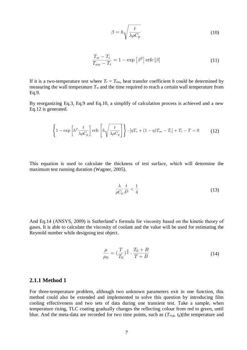
By reorganizing Eq.3, Eq.9 and Eq.10, a simplify of calculation process is achieved and a new

Eq.12 is generated.

(12)

This equation is used to calculate the thickness of test surface, which will determine the

maximum test running duration (Wagner, 2005).

(13)

And Eq.14 (ANSYS, 2009) is Sutherland’s formula for viscosity based on the kinetic theory of

gases. It is able to calculate the viscosity of coolant and the value will be used for estimating the

Reynold number while designing test object.

(14)

2.1.1 Method 1

For three-temperature problem, although two unknown parameters exit in one function, this

method could also be extended and implemented to solve this question by introducing film

cooling effectiveness and two sets of data during one transient test. Take a sample, when

temperature rising, TLC coating gradually changes the reflecting colour from red to green, until

blue. And the meta-data are recorded for two time points, such as (Tw,g, tg)(the temperature and

8

time when TLC displays green) and (Tw,b, tb)(the temperature and time when TLC displays blue).

h and Taw are constant in this transient test and can be determined by Eq.15-16.

(15)

(16)

Normally, two time series of data are sufficient to calculate local HTC and film cooling

effectiveness, but the random error might be high if two error point are selected. Therefore, to

reduce the random error, it is necessary to attempt to utilize all of the valid data and combine it

with least square method to figure out the global optimal. At every time point, the corresponding

temperature and hue could be put in to a Eq.15 and a series of Eq.15 could be produced for each

test. A MATLAB code will help to solve the unique local HTC and film cooling effectiveness.

2.1.2 Method 2

An alternative method is conducting two separate tests with the same mass flow for streams but

with different flow temperature. And set a certain color as the indicator.

(17)

(18)

(19)

In ideal condition, Taw is constant during a single transient test and the temperature at

mainstream inlet is able to achieve a step change from ambient to hot fluid. But it is not possible

in reality, and then the Taw becomes a function of time. The additional complication is modified

from Eq.9 by the idea of superposition and Duhamel’s theorem. Duhamel’s principle is a general

method for obtaining solution of inhomogeneous linear evolution equations, such as this heat

transfer equation.

2.1.3 Method 3

Both method 1 and method 2 assume that the driving temperature Taw is a constant and it could

achieve immediate change while hot air starts to contact with test surface. However, in real

9

condition, it might cost some time for the hot air to reach the test chamber after turning on the

valve, considering there is a volume between test chamber inlet and valve. For this reason, the

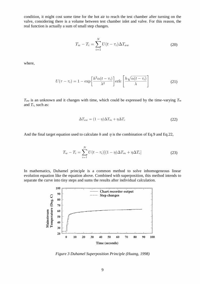
real function is actually a sum of small step changes.

(20)

where,

(21)

Taw is an unknown and it changes with time, which could be expressed by the time-varying Tm

and Tc, such as:

(22)

And the final target equation used to calculate h and is the combination of Eq.9 and Eq.22,

(23)

In mathematics, Duhamel principle is a common method to solve inhomogeneous linear

evolution equation like the equation above. Combined with superposition, this method intends to

separate the curve into tiny steps and sums the results after individual calculation.

Figure 3 Duhamel Superposition Principle (Huang, 1998)

10

2.1.4 Method 4

Another transient heat transfer model is modified from Dr.Drost,1998 assumes the coolant

temperature is a function of time. Therefore, when implementing Laplace transformation for wall

temperature, Tc will be transferred into s domain function.

(24)

2.2 Dimensional Analysis

To analyse the relationship between different physical quantities without the inference of unit’s

conversion, dimensional analysis is implemented to simply the process. This project intends to

validate the film cooling effectiveness and heat transfer coefficient for cylindrical holes.

Normally, the parameters for film cooling are divided in two type: one is based on the geometry

of cooling hole, like Reynold Number, and another depends on the flow properties, like Blowing

Ratio. In this case, four dimensionless quantities are chose, which are shown in Eq.25.

(25)

At the early stage of engineering experiment, it is expensive and unpractical to directly building

a real-size model for testing and similarity analysis is the alternative method to run the

experiment while make sure the result could be used as a reference.

2.2.1 Hole Geometry Based Distance (x/D, y/D)

Scaled with the hole diameter D, the downstream distance x/D is used to demonstrate the

streamwise dimensionless distance and the span-wise distance y/D is used to demonstrate the

span-wise dimensionless distance. Coupled with film cooling effectiveness or heat transfer

coefficient, these two parameters show how the film cooling air performers on the whole test

surface.

After the coolant hole, the coolant air starts to mix with hot gas and the film cooling

effectiveness decreases with the downstream distance, which could be plotted for better

visualization.

11

Figure 4 Surface Coordinate

2.2.2 Blowing Ratio (M)

Blowing ratio is a parameter which includes the flow’s density and velocity and it combines the

mass flux ratio of coolant air and hot gas. Blowing ratio is defined as:

(26)

where subscript c and m stand for coolant and mainstream respectively. As a decisive parameter,

blowing ratio is one of keys to design the film cooling test. According to Baldauf et. al. (Baldauf,

1997), the cross flow effect dominates at low blowing ratio and area near to coolant hole has a

high film cooling effectiveness, while the mixture air dominates at high blowing ratio and the

coolant has a better cooling performance at downstream area. In conclusion, the overall

effectiveness reaches maximum while blowing ratio is equal to zero.

2.2.3 Reynold Number (Re)

The Reynold number is most common dimensionless quantity in fluid dynamic which is

normally used for predicting flow patterns in various flow conditions. At low Re, the flow tends

to be laminar flow and turbulent flow happens while Re is high. The Reynold number is defined

as:

(27)

where 𝜌𝑐 is the coolant air density, 𝑉𝑐 is the coolant velocity, D is the coolant hole diameter, and

𝜇𝑐 is the coolant air dynamic viscosity. Beside the coolant hole based Re, the chamber hydraulic

diameter based Re is also a key value for designing this test.

12

2.3 Thermochromic Liquid Crystal

2.3.1 Thermochromic Liquid Crystal

Liquid crystals could be divided into two main categories based on how their parent solids’

complete molecular order breaks down and these two types are called Lyotropic and

Thermotropic. Lyotropic liquid crystals result from the action of a solvent, which could be used

for producing materials such as soaps, various detergents and polypeptides. And Thermotropic

liquid crystals are thermally activated material and it made by heating the mesogenic solids up to

a certain temperature to melt (Hallcrest, n.d.).

According to structural viewpoint or molecular order, Thermotropic liquid crystals could be

further classified into Smectic liquid crystals and Nematic liquid crystals, where the molecule

axes of both cyrstals are parallel to each other. But Smectic’s molecular centers of gravity

arrange in layers which move in two-dimensional planes and Nematic’s molecular gravity

centers move in three-dimensional coordinate.

For Nematic liquid crystals, it could be divided into two subcategories: Non-Optically-Active

(Nematic/non-twisted) and Optically-Active (Cholesteric/twisted). Sometimes, Cholesteric can

be categorized as same hierarchy as Smectic and Nematic, but strictly speaking, Cholesteric

liquid crystal is a special type of Nematic whose physical properties make it necessary to be

classified as Nematic thermodynamically.

Figure 5 Liquid Crystals Classification (Hallcrest, n.d.)

Thermochromic Liquid Crystal (TLC) is special type of liquid crystals, which react to changes in

temperature by changing color, and all of TLCs belongs to Cholesteric type, whether sterol-

derived, non-sterol or a mixture of the two. TLCs have chiral molecular structure and are

Optically-Active organic chemicals’ compound.

13

Figure 6 displays the phase changes of TLC with temperature increasing. Initially, the solid

crystal molecules are well organized and molecules in each layer have the same orientation.

While the temperature climbing, the cholesteric liquid crystal molecules start to twist to a certain

direction and the twisting angle will keeps increase. For example, the first layer molecules head

to left and the send layer molecules will spin a certain angle clockwise. Then the next layer

molecules will spin the same angle clockwise based on the previous layer direction until the last

layer molecules go back to the same orientation as the initial position. The distance between the

first layer and the last layer is pitch length. When a beam of unpolarized while light enters this

texture, it is selectively polarized, and TLC reflects a certain color. Although all of changes are

thermally reversible, the heat process will accelerate the aging of TLC. Therefore, it is necessary

to implement recalibration after 5-10 runs and limit the number of times of experiments.

Figure 6 TLC Phase Changes with Temperature Changing (Hallcrest, u.d.)

By selectively reflecting incident white light, TLCs indicate temperature by color shifting. A

breakdown of TLC into temperature-sensitive and shear-sensitive, is divided based on how many

colors could be shown. The original condition of TLC is colorless, and it will gradually show the

color as the temperature increasing against a black paint background.

Temperature-sensitive starts at transparent condition and passes through colors from visible light

spectrum in sequence before fading out at a high temperature. As temperature cooling down, the

color change sequence is reversed from blue to red. There are four key points for each TLC

formula: Red Start, Green Start, Blue Start and Clearing Point where TLC returns colorless. The

14

most important property for TLC is the band width which is defined as the temperature range

between the Red Start and Blue Start e.g. R28C10W describes that the red color starts at 28oC

and the blue color starts 10oC higher at 38oC. Red Start could locate between -30oC and 120oC,

and band width varies between 1oC and 10oC.

Figure 7 Temperature-sensitive TLC Color Spectrum (Hallcrest, n.d.)

Different from temperature-sensitive mixtures, shear-sensitive mixture, also called temperature-

insensitive, is only able to display one single color below Clearing Point. For example, R45C

indicates that a mixture shows red below its Clearing Point at 45oC.

Figure 8 Temperature-insensitive TLC Color Spectrum (Hallcrest, n.d.)

2.3.2 RGB Theory

The RGB color model is an additive color model where different portions of red, green and blue

light are mixed together and is represented by three values. It is device-dependent color theory

and chromatic aberration is inevitable where calibration is required before experiments to make

compensation for R, G, B values.

In this project, we selected a Blackmagic CCD-camera as the sensor to capture RBG values.

Charge-coupled device, abbreviated as CCD, is an integrated circuit with many neatly arranged

capacitors that sense light and convert the image into digital signals. Through the control of the

15

external circuit, each small capacitor can transfer its charge to its adjacent capacitor. CCD is

widely used in digital photography, astronomy, especially optical telemetry (photometry), optical

and spectral telescopes, and high-speed photography such as lucky imaging. For every CCD

camera, its top left channel is called ‘starting channel’ and it will determine this camera’s

demosaicing method. There are totally four types of combination of RGB channels: RGGB,

BGGR, GBRG and GRBG.

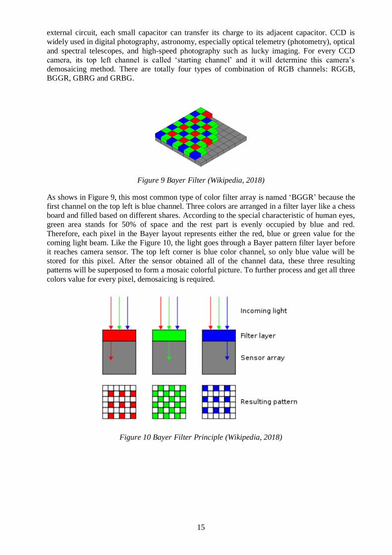
Figure 9 Bayer Filter (Wikipedia, 2018)

As shows in Figure 9, this most common type of color filter array is named ‘BGGR’ because the

first channel on the top left is blue channel. Three colors are arranged in a filter layer like a chess

board and filled based on different shares. According to the special characteristic of human eyes,

green area stands for 50% of space and the rest part is evenly occupied by blue and red.

Therefore, each pixel in the Bayer layout represents either the red, blue or green value for the

coming light beam. Like the Figure 10, the light goes through a Bayer pattern filter layer before

it reaches camera sensor. The top left corner is blue color channel, so only blue value will be

stored for this pixel. After the sensor obtained all of the channel data, these three resulting

patterns will be superposed to form a mosaic colorful picture. To further process and get all three

colors value for every pixel, demosaicing is required.

Figure 10 Bayer Filter Principle (Wikipedia, 2018)

16

2.3.3 HSV Theory

After obtained all RGB value for every pixel, it is time to transfer the RGB value into HSV value.

The HSV color model is a quite common color model which is represented points in the RGB

color model in a cylindrical coordinate system. It is more intuitive than the geometry based on

the Cartesian coordinate system RGB. HSV stands for hue, saturation and value respectively.

Most TVs, monitors, and projectors produce different colors by mixing different colors of red,

green, and blue light. This is the additive color method for the three primary colors of RGB. In

this way, a large number of different colors can be generated in the RGB color space, however,

the relationship between the values of the three colors components and the generated color is not

intuitive.

The HSV describes a color as a point in the cylindrical coordinate system. The center axis of the

cylinder takes the value from the black at the bottom to the white at the top and the gray in the

middle. The angle around this axis corresponds to the ‘hue’ to the axis. The distance corresponds

to "saturation" and the height along this axis corresponds to ‘value’.

Figure 11 HSV Cylinder (Wikipedia, 2019)

Assume (r, g, b) is the red, green, and blue coordinates of a color, respectively, whose values are

real numbers between 0 and 1. Set max is equivalent to the largest value among R, G and B and

min is equal to the smallest value among these values. To find the (h, s, v) value in the HSV

space, where h ∈ [0, 360) degrees is the hue angle of the angle, and s, v ∈ [0, 1] is the saturation

and value, the equations are:

(28)

17

(29)

(30)

In this project, a build-in MATLAB function rgb2hsv is selected as tool to transfer RGB color

model to HSV color model and only hue value will be left for further calculation.

Besides, HSV can also be conceptually considered to be the inverted cone of color (black at the

lower vertex, white at the center of the upper bottom). On the top hexagonal surfaces, hue starts

at red color with 0 degree and its value increases with counterclockwise movement passing

colors spectrum from yellow, green to blue, magenta. For a certain angle, the farther this point is

from center axis, the higher the saturation this color is.

Figure 12 HSV Cone (Marques, 2011)

2.3.4 Hue-Temperature Distance Weight

In this project, we can only find the relationship between hue and temperature in the area near

TCs. But it is important to find a way to generalize the relationship reasonably and help any

other points on the surface figure out their individual correlations.

Take Figure 13 as a sample, we are able to measure the temperature at point a - i where surface

thermocouples are located. However, this thesis is more interested on the temperature at center

point like P and the integrity of this area would be destroyed if inserting thermocouple at this

location. Hence, thermocouple can only exist outside the research area.

Even though we are unable to directly measure the accurate temperature at point P, it is possible

to use the temperature values at point a - i to estimate the temperature P. because all of the points

are in the same Cartesian coordinate system, it is able to find 3 closest points for P. In this

sample, i, e and h are the closest points and the distances between them and P are Di, De and Dh.

The next step is to weight their temperature value by distance and the closer the point is, the

higher weight it will get.

18

(31)

Figure 13 TLC Distance Weight Method

a

c

b

d e f

g

h i

P

19

3 EXPERIMENT PROCESS

3.1 Pre-setup

3.1.1 Test rig

Figure 14 shows the layout of the test cell set-up. This film cooling test rig is located at Fluid

Dynamics Laboratory at Siemens Industrial Turbomachinery AB in Finspång. This test rig is

divided into two part: the block inside the dash-line rectangular is located in a dark cell with

blocked window; the rest part is directly connected with the laboratory.

The mainstream flows through a 70mm diameter pipe and passes an orifice after two on/off

valves which is used to measure the main mass flow. The orifice is between two flanges with an

outer diameter of 114mm and an inner diameter of 12.48mm. After the orifice, the flow goes

through an electric resistance heating element inside the pipe which is controlled by a PID-

controller, and a calibrated PT100 is inserted through the pipeline wall after the heater. Located

inside the test cell, Valve 3 could adjust the main flow to the design mass flow. The manometer

next to the Valve 3 indicates the pressure inside the main flow pipe and the pressure should be

lower than a defined value for safety reason. Before reaching the test object, the flow is guided to

a three-way valve which is connected to a control box on the desk outside. Under normal and

initial circumstances, the flow is directed to the atmospheric environment from the bypass. While

the main flow has been heated to the desired temperature, the switch on the control box is

triggered and it turns the flow direction from atmosphere to the test object.

A plastic hose connects the coolant air to the coolant chamber where the flow is evenly

distributed into five streams and ejected from five coolant channels. Then the coolant forms a

thin layer above the test surface and mixes with hot air. After passing the test object, the mixture

flows through a silencer and goes back to the atmosphere.

The test object is surrounded by four halogen lamps with 2900K color temperature which will be

used to adjust camera’s color balance. In order to homogeneously illuminate the test surface, it is

necessary to take some measures because uneven illumination will have impact on the accuracy

of result. Around the test object, a wooden structure box (80cm x 70cm x 60cm) caps the whole

test chamber and its four sides are wrapped up with diffusive paper. By this method, the incident

light from four lamps will be diffused and be uniformly distributed on the surface. The up side of

the box is covered with a black cloth so as to avoid light reflection from the mirror face above

the test surface.

20

Figure 14 Test Rig Layout

3.1.2 Test object

The test object is made up of two pieces and they are bolted together with thirty connection

points. To avoid flow leakage influencing the hydraulic Reynold Number, a layer of gasket is put

in the middle of two components and it perfectly coves all of the overlapping area. The whole

chamber is additive manufactured by PA2200, a fine-powder on the basis of polyamide 12, and

its thermal conductivity in direction vertical to sintered layer is 0.144 W/mK. In the two sides of

test chamber, two holes are drilled as the inlet and the outlet of air separately. For optical

accessing and camera recording, the top cover’s transparency is critical to the entire experiment.

Therefore, a transparent polycarbonate plate is selected as the test object’s top cover. The inner

frame dimension of the test chamber is 150 mm (Width) x 320 mm (Length) x 97 mm (Height)

and five 10mm diameter coolant channels with length of 100mm tilt towards the main chamber.

Figure 15 Sectional View of Test Chamber and Flow Direction

21

The thickness of bottom plate is quite critical for the whole experiment which determines the

maximum test duration. In this case, to achieve at least half minute test, the flat plate should have

at least 75mm of thickness and the calculation is based on the thermal properties of

manufacturing material. Deriviated from Eq.13, Eq.32 is used to calculate the maximum test

duration.

(32)

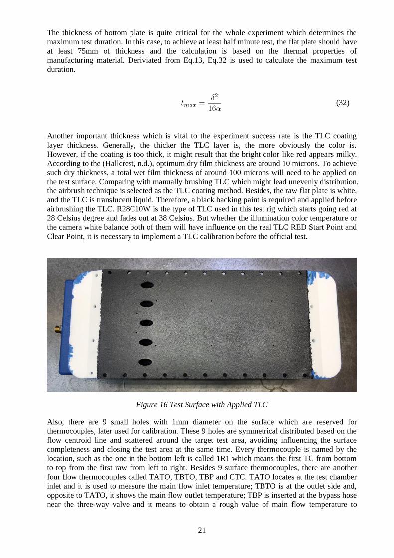
Another important thickness which is vital to the experiment success rate is the TLC coating

layer thickness. Generally, the thicker the TLC layer is, the more obviously the color is.

However, if the coating is too thick, it might result that the bright color like red appears milky.

According to the (Hallcrest, n.d.), optimum dry film thickness are around 10 microns. To achieve

such dry thickness, a total wet film thickness of around 100 microns will need to be applied on

the test surface. Comparing with manually brushing TLC which might lead unevenly distribution,

the airbrush technique is selected as the TLC coating method. Besides, the raw flat plate is white,

and the TLC is translucent liquid. Therefore, a black backing paint is required and applied before

airbrushing the TLC. R28C10W is the type of TLC used in this test rig which starts going red at

28 Celsius degree and fades out at 38 Celsius. But whether the illumination color temperature or

the camera white balance both of them will have influence on the real TLC RED Start Point and

Clear Point, it is necessary to implement a TLC calibration before the official test.

Figure 16 Test Surface with Applied TLC

Also, there are 9 small holes with 1mm diameter on the surface which are reserved for

thermocouples, later used for calibration. These 9 holes are symmetrical distributed based on the

flow centroid line and scattered around the target test area, avoiding influencing the surface

completeness and closing the test area at the same time. Every thermocouple is named by the

location, such as the one in the bottom left is called 1R1 which means the first TC from bottom

to top from the first raw from left to right. Besides 9 surface thermocouples, there are another

four flow thermocouples called TATO, TBTO, TBP and CTC. TATO locates at the test chamber

inlet and it is used to measure the main flow inlet temperature; TBTO is at the outlet side and,

opposite to TATO, it shows the main flow outlet temperature; TBP is inserted at the bypass hose

near the three-way valve and it means to obtain a rough value of main flow temperature to

22

estimate the start time; CTC is inserted into the coolant chamber through left side well and it

measures the coolant flow temperature. As shows in Figure 18, the heat conductivity of

thermocouple may have influence on the heat transfer coefficient of surrounding area, but it

could be ignored because the test surface is thin.

Figure 17 Thermocouple Arrangement

Figure 18 Lateral View of Test Surface

On the both two sides of the test chamber, three holes with 1.6mm are drilled and each of them is

filled with a pressure tap, directly connected by a transparent plastic hose to a digital pressure

measurement system. All of the six pressure taps are located at the same height and expected to

obtain relatively same pressure value. The pressure differences between each hole indicate

pressure drops along the streamwise and the lower the value is, the more accurate the test results

get. Besides, another two pressure taps from this pressure system located on the flanges on two

sides of the orifice, measuring the main mass flow by calculating pressure drops. A standard

atmospherical pressure devise is introduced into this system as reference.

23

3.1.3 Measurement equipment

It’s necessary to build a data acquisition system and use it to collect all the measurement

information. RigView is an in-house software which is able to organize data from various inputs

and gather them into a DIF format file. Besides the data collection function, it could also display

the real-time data during the test, which is quite convenient for lab stuff to check test conditions.

Normally, a DATASCAN 7220 16-channel measurement processor and a NetScanner System

Model 9116 are directly connected with computer via USB or ethernet. The data imported from

these two data logs will be read by RigView and displayed on screen by a user interface.

The DATASCAN records the voltage changes from all of the thermocouples and estimates the

temperature according to the thermoelectric effect. For the NetScanner, it is a pressure

measurement system whose outcomes are calibrated by a standard reference – a ROSEMOUNT

absolute pressure transmitter.

Figure 19 NetScanner and DATASCAN

3.2 Experiment

In this project, the test section could be divided into three parts according to the independence:

thermocouple calibration, thermochromic liquid crystal calibration and heat transfer experiment.

All of them are listed chronologically. First, thermocouple is the basic temperature measurement

equipment and its accuracy controls the uncertainty of the experiment results. Then, the correct

correlation between color hue value and temperature is vital for the utilization of TLC. After

knowing how colors correspond to temperatures, a flat plate transient heat transfer experiment

can be run to evaluate the performance of the film cooling and estimate the heat transfer

coefficient.

3.2.1 Thermocouple Calibration

As mentioned previously, the accuracy of the thermocouple is the fundamental of a success

experiment. Therefore, a standardization is required before mounting them. First, a reference PT-

100 is selected and calibrated by the Technical Research Institute of Sweden, a third-party

professional organization. Then bundle all the type K thermocouples with this PT-100 tightly

24

and put them into a thermos bottle with hot water. Guarantee their tips roughly at the same water

depth and a mixture of water is necessary to make sure that all the tips are surrounded by the

water at the same temperature. In best condition, an electrical cap mixer is utilized, but the extra

length of the PT-100 limits the application of the electrical cap. For this reason, a manually

mixture step is implemented during the entire calibration.

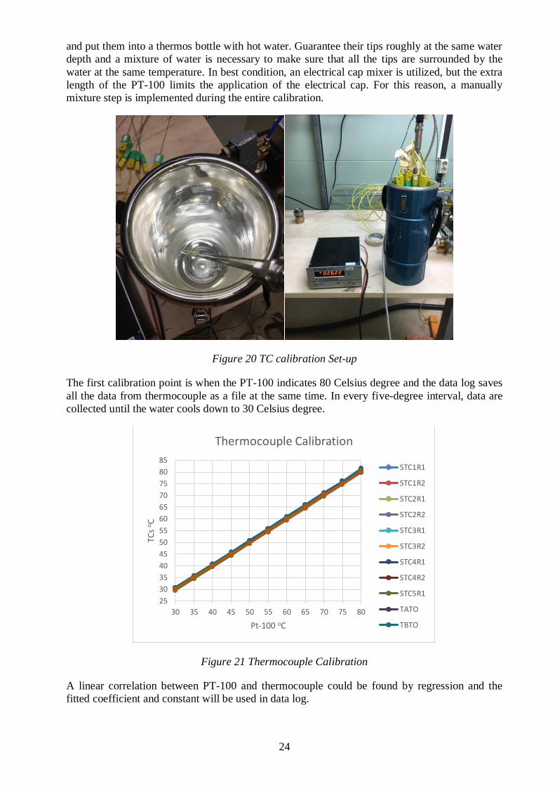
Figure 20 TC calibration Set-up

The first calibration point is when the PT-100 indicates 80 Celsius degree and the data log saves

all the data from thermocouple as a file at the same time. In every five-degree interval, data are

collected until the water cools down to 30 Celsius degree.

Figure 21 Thermocouple Calibration

A linear correlation between PT-100 and thermocouple could be found by regression and the

fitted coefficient and constant will be used in data log.

25

30

35

40

45

50

55

60

65

70

75

80

85

30 35 40 45 50 55 60 65 70 75 80

TCs

oC

Pt-100 oC

Thermocouple Calibration

STC1R1

STC1R2

STC2R1

STC2R2

STC3R1

STC3R2

STC4R1

STC4R2

STC5R1

TATO

TBTO

25

3.2.2 Thermochromic Liquid Crystal Calibration

This project intends to explore the heat transfer coefficient and film cooling effectiveness and the

wall temperature on the entire surface is the core of the HTC calculation. Normally,

thermocouple would be a good choice for point temperature measurement, but this test needs to

map the temperature on the whole surface. Thermochromic liquid crystal is applied on the

surface to indicate various temperatures by changing colors and the correlation between colors

and temperatures is key of this project. To figure out the internal connection between hue and its

corresponding temperature, a calibration of thermochromic liquid crystal is implemented.

The calibrated thermocouples in previous step will be inserted in the flat plate from the back side,

and their tips will exactly at the flat plate surface, which means to assume that the thermocouples

measure the surface temperature around a small area. At a certain time, this test makes an

assumption that this small area’s average hue indicates the temperature measured by the

corresponding thermocouple. Therefore, after a successive relating between hues and

temperature at the same time, a fitted curve could be obtained and used for further heat transfer

experiment.

Figure 22 Temperature and Hue Correlation

In this calibration, a steady-state experiment is carried out by using main flow to gradually heat

up the test surface. Every raise of heater’s temperature setting needs dozens of minutes to

achieve evenly and steady temperature distribution. After the surface is heated to a steady

condition, data log will start to collect temperature data and pictures will be taken at the same

time. Later inside the MATLAB, temperature data will be correlated with corresponding hue

value and the correlation will be used in transient experiment.

3.2.3 Heat Transfer Experiment

After two calibration experiments, the correlation between hue and temperature has been found

and it would be used in the heat transfer experiment to indicate local point temperature on the

entire test surface. Figure 23 shows how the test chamber looks like during one transient test.

0.1

0.2

0.3

0.4

0.5

0.6

0.7

26 27 28 29 30 31 32 33 34 35 36 37 38 39 40 41 42 43 44 45 46

Hu

e [-

]

Temperature oC

Temperature-Hue Correlation

1R1

1R1

2R1

2R2

3R1

3R2

4R1

5R1

26

Before the experiment, a safety check is implemented. It has to make sure that all of the on/off

valves have been closed and the three-way valve has been switched to bypass direction. Check

whether sensors are well connected, and test object is well fixed.

Figure 23 Transient Test Object

Then gradually turn on the main flow pipe valve and coolant hose valve until the mass flows

reach designed values by observation. A heater controlled by a self-made PID-controller starts to

heat the mainstream up to 55 Celsius degree, based on TBP value. While the main flow

temperature has climbed to design value, it is time to start recording test data by CCD-camera

and data log. Switch the three-way valve and guide the main flow to test object instead of bypass.

After the maximum running time, turn off sensors and switch back the three-way valve. Let the

test object naturally cool down to ambient temperature. To avoid environment influence and

guarantee the filmed imaged showing the heat-up process, heat transfer experiment can only be

carried out once per day. After stopping the experiment, all of the data will be imported into

MATLAB for postprocessing.

3.3 Post-process

After a series of experiment, the data required for calculation are sufficient. To better utilizing

the data, several postprocess steps are implemented:

1. Collect all the information from camera and data scanner

2. Import the RAW image and temperature data in to MATLAB

3. Transfer RGB to HSV and denoise

4. Calculate the HTC and film cooling effectiveness for every pixel within target

surface

27

3.3.1 Data collection and transformation

The first step of postprocess is to collect experimental data from various sensors. The most

important data are the RAW images from CCD-camera with a resolution of 1920px * 1080px.

Normally, one transient test will generate 300 frames of digital negative files with 0.1s interval.

To be recognized by MATLAB, all of the images has to be processed by Adobe DNG Converter

and be transferred from RAW format to DNG format. According to (Sumner, 2014), to display

an image on a screen, the RAW format image needs to be linearized, white balanced,

demosaiced and color space corrected. The below picture shows the work flow of transferring

RAW data into usable MATLAB data.

Figure 24 Workflow of Transferring from RAW to MAT

Besides the RAW images, temperature information from RigView is another crucial data for the

entire experiment. The data exported from RigView will be in ascii format and each column

records time-series data from a certain thermocouple. There is a column called Switch which is

used to indicate the condition of three-way valve. If the Switch shows 1, it means that the main

flow is guided to test chamber; if it shows 0, it means that the flow passes through the bypass

and goes to the ambient environment. Therefore, this test only needs the rows where Switch is 1.

Inside the DIF file, pressure drops between several pressure taps are recorded during the whole

test to check whether leakage exist. Also, coolant mass flow and mainstream mass flow are part

of the main content which will be used for solver.

3.3.2 Denoising

Later inside MATLAB, the data from RBG channels will be extracted and transferred into HSV

format. Only hue value could be saved and utilized. However, the noisy signal will dramatically

influence the accuracy of the solver’s results. Denoising is implemented before the hue value is

put into series of equations. As shows in Figure 25, the black widely fluctuated cure is the raw

hue directly obtained from images, obviously which is not suit for calculation. Because the

surface temperature keeps climbing since time = 0, the hue should also stay continuously

growing. The hue for this recording time needs to be higher than the value from the previous

recording time. A negative gradient would lead to a negative HTC, which is not expected.

28

Figure 25 Hue Denoising Process

Wavelets is a decent choice to smooth the hue data. Based on Fourier transformation, wavelets

provides more possibility of storage both signal’s amplitude and time. Fourier transformation

means to fix the signal changing with time. The short-term Fourier transformation uses a certain

width window to divide the changing signal into several parts and applies Fourier transformation

for each part. The Wavelet replaces an infinite sine wave with a wavelet that attenuates and

transforms the non-periodic signal. In the previous project, Wavelet transform is used to denoise

the signals of each RGB channels. Wavelets is the tool of denoising, and it performs quite well.

However, in this case, a more robust and more simple method is utilized – the moving average

filter. Besides, the moving average filter is optical for reducing random noise or extreme outlier,

which is exactly the problem faced in this project. The main concept for this filter is to replace

the value with a mean within a range fixed moving window. The blue curve is the filtered hue

values, and its fluctuation amplitude is decreased comparing with original curve. Then the

filtered hue is curve fitted by a custom sigmoid function that is selected to guarantee the single

increasing trend. The data on the red curve will be saved and used for next step. Figure 25 is a

sample pixel and every pixel on the test surface will go through all the above processes.

3.3.3 Solver

Each local HTC on test surface corresponds to a local driving fluid temperature and a local wall

temperature. As described previously, the local wall could be got by TLC, but no indicator is

able to display real-time local driving temperature. A rough estimation by distance weighting

between inlet and outlet temperatures is implemented and it also assumes that the span-wise

points with same y-coordinate value share one driving temperature.

29

Figure 26 Local Driving Temperature Calculation

Figure 27 Solver Workflow for One Pixel

30

Figure 27 displays the whole work flow of solver built in MATLAB. Two initial guess values of

HTC and film cooling effectiveness are given, and they are used for starting the iteration process.

Based on the experimental assumption, HTC and film cooling effectiveness are constants for a

certain point during the whole experiment duration. For a certain pixel point, a corresponded

temperature and time information are put into the same equation, which form an equation set. By

partial deriving and transposing, the value of HTC and film cooling effectiveness are updated

with each iteration until the residence is lower than a certain tolerance error.

The final HTC and film cooling effectiveness for a certain pixel will be stored in two two-

dimensional matrixes whose coordinates are used for positioning this pixel. After finished the

calculation for this pixel, the initial guess will be reset, and iteration starts again until the matrix

is fully filled.

31

4 RESULTS AND DISCUSSION

4.1 Calibration

As explained in previous chapter, two calibration tests are implemented in this project: the first

intends to calibrate the surface and flow thermocouples by a standard Pt-100; the second means

to calibrate the Thermochromic Liquid Crystal and correlate its hue with surface thermocouple’s

values. The key concept of calibration is to use a particular sensor to figure out the relationship

between inputs and outputs

According to the Figure 21, it is obviously that the two variable has a linear relationship and

their coefficients could be obtained by linear regression. The dependent variable TC Voltage and

the independent variable Pt-100 value are imported into MATLAB curve fit toolbox and it

automatically generates the C0 and C1 for each thermocouple.

(33)

Table 1 shows the linear regression outcomes and these data will be used in RigView’s channel

mapping. Then the DIF generated by this in-house software will directly export the correct

temperatures.

Table 1 Thermocouple Calibrated Coefficients

TC C0 C1 TC C0 C1

1R1 0.5611 1.0143 4R1 0.7928 1.0073

1R2 0.6861 1.0136 5R1 0.5778 1.0063

2R1 0.6497 1.0143 CTC 0.4377 1.0187

2R2 0.7159 1.0143 TBP 0.7858 1.0088

3R1 0.6738 1.0092 TATO 0.2316 1.0284

3R2 0.6462 1.0139 TBTO 0.2344 1.0199

Normally, every TLC has a unique color spectrum, but the illumination condition and the camera

setting would both have impact on it. Therefore, it is necessary to apply a calibration to reduce

environmental influences and fix the lighting condition.

Another important calibration outcome is from Thermochromic liquid crystal color calibration,

where we get a clear understanding of the correlation between color hue and corresponding

temperature.

32

Table 2 lists the coefficients fitted by 5 order polynomial function and these data will be stored

in to matrix for transient test.

Table 2 Thermochromic Liquid Crystal Calibrated Coefficients

TC P5 P4 P3 P2 P1 P0

1R1 10040 -24890 23340 -10400 2224 -153

1R2 15490 -36080 32700 -14380 3080 -227

2R1 3174 -10180 10840 -5150 1138 -65

2R2 -3659 352 5233 -4114 1177 -87

3R1 104400 -228600 198900 -85840 18380 -1531

3R2 136800 -304200 269100 -118200 25790 -2205

4R1 -130700 235700 -167500 58680 -10130 719

5R1 121900 -264900 228100 -97250 20540 -1690

This is the 5-order polynomial fitting function used in MATLAB code.

(34)

33

4.2 Transient Heat Transfer Experiment

Figure 28 displays the final result of HTC and film cooling effectiveness in a two-dimensional

color map. The x-axis is the ratio of streamwise distance and hole diameter, and y-axis is the

ratio of span wise distance and hole diameter D. The brighter color the dot is, the higher the

value of HTC and film cooling effectiveness is. And the white space means data lack at these

points. This target area is exactly the space after coolant ejected and (0,0) is the coordinate for

the first pixel point after center coolant hole.

Figure 28 HTC and Film Cooling Effectiveness Map

It is obviously that the coolant performs well just after it is ejected from hole and these two

values reach maximum. With streamwise distance increasing, the hot air keeps mixing with

coolant air and the temperature of driving fluid continuously climbing high until it up main flow

temperature. For this reason, these two target values decrease with distance increasing and it is

reasonable that the coolant is unable to reach the points close to the outlet. Also, the heat transfer

coefficient and film cooling effectiveness seem to have a very similar distribution pattern with

the same increase and decrease trend. Ideally, the points with the same x-axis coordinate should

have the same HTC and film cooling effectiveness, based on the homogeneous flow distribution

assumption. But the result implies that there are still some vertexes existed and they change the

flow direction. Another guess is that the flow runs to the side wall and be rebounded back.

Even the span wise heat distribution is an interesting research topic, this project is focus on the

streamwise coolant performance. Hence, the heat transfer coefficient and film cooling

effectiveness are summing averaged on y-axis.

34

Figure 29 Span Wise Average

The blue line is average HTC and film cooling effectiveness and the orange line is the data

obtained from validation paper (Yu, 2002) while Blowing ratio is 1 and Reynold number is 2300.

Unexpectedly, the curves of the two colors do not overlap with each other, even they have a

similar trend. To figure out what the problem inside, the exhaustion method is implemented by

feeding various values of HTC and film cooling effectiveness in one-pixel heat transfer equation

to calculate the residuals.

Figure 30 Residual of Exhaustion Method

35

As Figure 30 indicated, there are a lot of per of solution for one pixel and it is almost unable to

pick up an optimal solution considering the solver is easy to stop at local minima. But we could

see that the heat transfer coefficient tends to be stable with film cooling effectiveness increasing.

Considering the unevenly distributed flow, there might be some data that do not fit the basic

assumption, such as the beginning sector (the first short sector in Figure 31). The results shown

above are generated based on method 1 and all of the data points on the red curve have been

utilized for calculation. Therefore, the data in the first several seconds might be the original of

validation failure. To further improved the data quality, we should only use data from the last

several seconds like the short red section at the right side of the picture. It is possible to validate

the guess by sliding data import window and comparing the results.

Figure 31 Hue for One Pixel

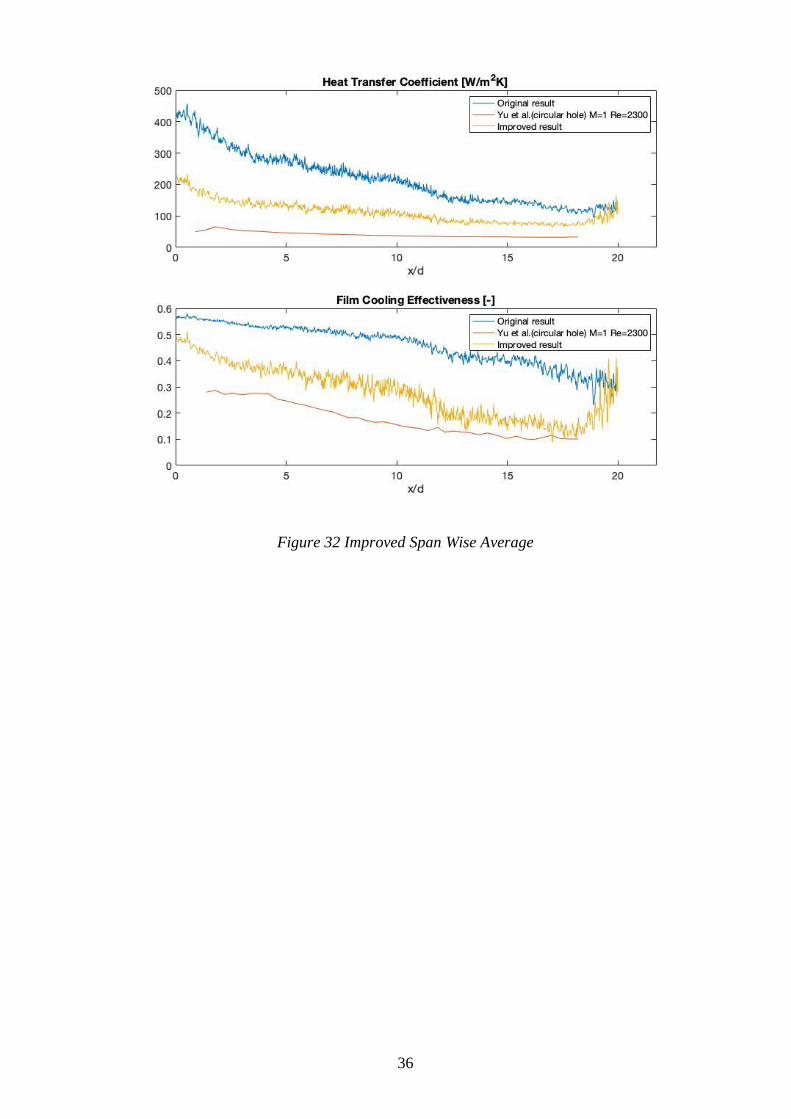
By only calculating the last five seconds data, two improved curves are generated in Figure 32,

where blue curve is the original results, orange curve is from validation paper and yellow curve

is the improved results. As it shows, the heat transfer coefficient shrinks to half of the original

data around the hole area and the slope keeps flatting with streamwise distance increasing. While

x/d =20 or close to the exhausting outlet, the HTC value of these curve of two colors almost

reach the same level, which could be explained by the same driving temperature. As illustrated

above, with the x/d ratio increasing, less coolant air could flow to this area, so the driving

temperature tends to be close to the hot air temperature. Although the film cooling effectiveness

does not reduce by half, it still shows an obvious drop, especial in the middle area. Both of the

objects have partially matched the expectation, but there are still some aspects that could be

improved further, such as the TLC band-width selection. The trend for global minima is obvious

but unfortunately, the experiment hasn’t reached the point before the test end within 30s which is

the test duration limitation. If the thickness of the test object increases, each test could run for a

longer time which will provide a more stable flow. It is tricky to verify whether the hot air has

become fully developed flow by calculation or observation. It needs to mention that all of the

data are obtained from the experiments with the same blowing ratio =1 and hole-based Reynolds

number = 2300.

36

Figure 32 Improved Span Wise Average

37

5 UNCERTAINTY AND CONCLUSIONS

5.1 Uncertainty

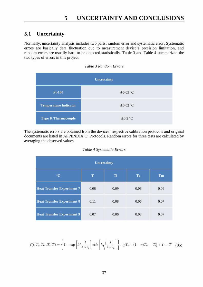
Normally, uncertainty analysis includes two parts: random error and systematic error. Systematic

errors are basically data fluctuation due to measurement device’s precision limitation, and

random errors are usually hard to be detected statistically. Table 3 and Table 4 summarized the

two types of errors in this project.

Table 3 Random Errors

Uncertainty

Pt-100 ±0.05 °C

Temperature Indicator ±0.02 °C

Type K Thermocouple ±0.2 °C

The systematic errors are obtained from the devices’ respective calibration protocols and original

documents are listed in APPENDIX C: Protocols. Random errors for three tests are calculated by

averaging the observed values.

Table 4 Systematic Errors

Uncertainty

oC T Ti Tc Tm

Heat Transfer Experiment 7 0.08 0.09 0.06 0.09



(35)

38

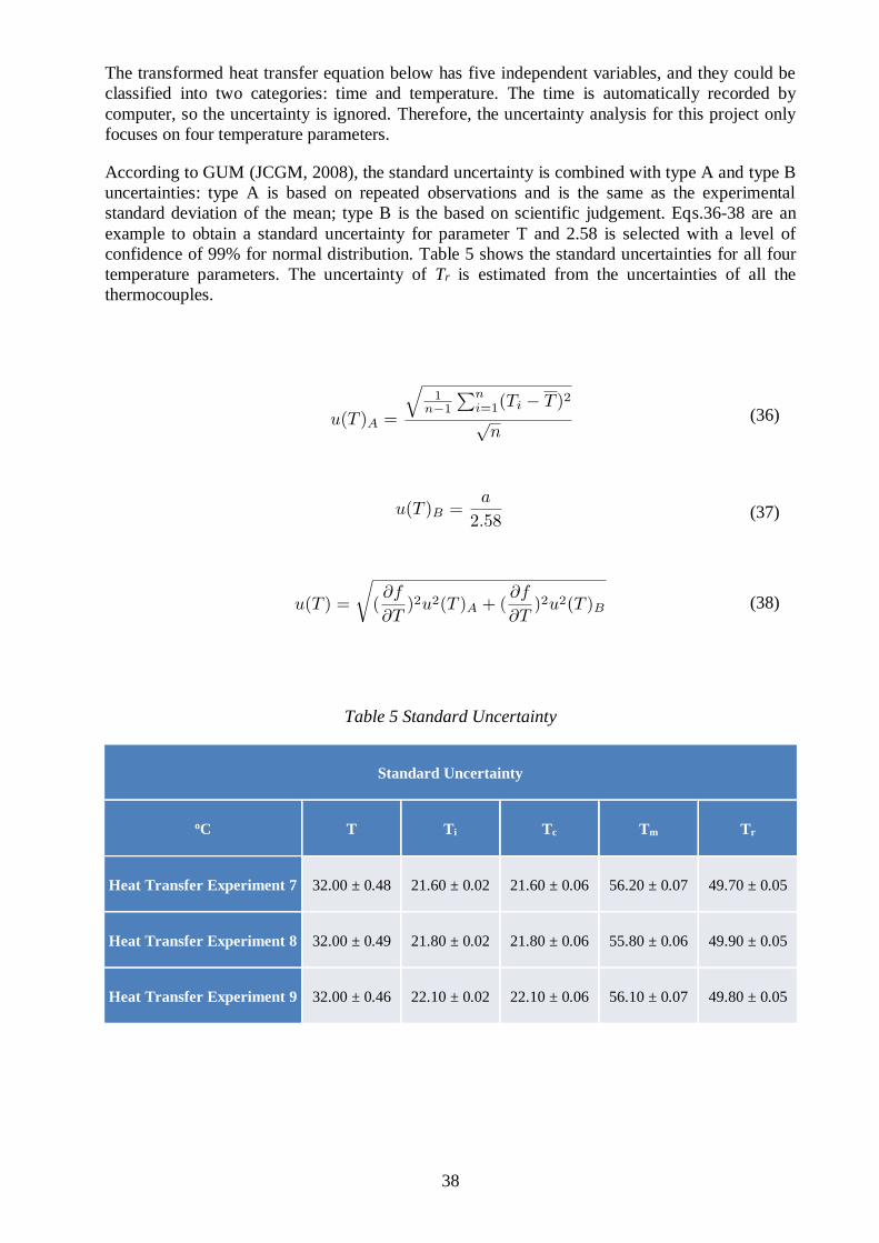
The transformed heat transfer equation below has five independent variables, and they could be

classified into two categories: time and temperature. The time is automatically recorded by

computer, so the uncertainty is ignored. Therefore, the uncertainty analysis for this project only

focuses on four temperature parameters.

According to GUM (JCGM, 2008), the standard uncertainty is combined with type A and type B

uncertainties: type A is based on repeated observations and is the same as the experimental

standard deviation of the mean; type B is the based on scientific judgement. Eqs.36-38 are an

example to obtain a standard uncertainty for parameter T and 2.58 is selected with a level of

confidence of 99% for normal distribution. Table 5 shows the standard uncertainties for all four

temperature parameters. The uncertainty of Tr is estimated from the uncertainties of all the

thermocouples.

(36)

(37)

(38)

Table 5 Standard Uncertainty

Standard Uncertainty

oC T Ti Tc Tm Tr

Heat Transfer Experiment 7 32.00 ± 0.48 21.60 ± 0.02 21.60 ± 0.06 56.20 ± 0.07 49.70 ± 0.05



39

According to Eq.2, film cooling effectiveness is a function of Ti Tc and Tm, so its uncertainty

could be calculated by Eq.39. Based on the same principle and Eq.12, Eq.40 is used to calculate

the uncertainty of heat transfer coefficient. Table 6 shows the uncertainties of film cooling

effectiveness and heat transfer coefficient from three experiments.

(39)

(40)

Table 6 Uncertainty of h and

Uncertainty

h [W/m2K] [-]

Heat Transfer Experiment 7 151.20 ± 0.22 0.19 ± 0.06



5.2 Conclusions

The main purpose of this thesis is to explore the film cooling performance at a certain condition

and the heat transfer coefficient and film cooling effectiveness are the objective of this project.

All of the experiment setting or measurement serve for this target. Thermochromic Liquid

Crystal is the tool of temperature measurement instead of other sensors like thermocouple. But

the thermocouple still holds an important role inside this test rig. The MATLAB code and the

test rig setup are upgraded based on new requirements and a totally new methodology is

introduced comparing with previous study at SIEMENS Fluid Dynamic Lab. The major

difference and the biggest improvement is adding of the coolant air which dramatically increased

the difficulty of data processing and solver.

Based on the existing test cell, a coolant air pipe is introduced, and the test object is redesigned

based on Reynold number = 2300 and Blowing ratio = 1. A different thermocouple mounting

method is implement and two different calibration experiments has been run before the transient

heat transfer test. The 12 thermocouples are calibrated by a standard Pt-100 and the band-width

40

of Thermochromic Liquid Crystal is R28C10W. To guarantee that both of the calibration data

are trustworthy, every test mentioned are taken in-situ.

CCD-camera is used to capture the TLC’s hue changing with time and it could be treated as a

noisy signal needing smoothing. Therefore, several image processing steps are applied before the

pictures could be readable. Then transfer the RGB color into HSV model and use the hue value

to indicate the wall temperature which is the most important variable in heat transfer. The

improved final method selects the last 5 seconds’ data set and combines them with least square

method to iterate optimal heat transfer coefficient and film cooling effectiveness for a certain

pixel. Repeat the process until every pixel on the surface are visited.

This project’s ultimate goal is to simulate the same film cooling situation in (Yu, 2002). And the

final results prove that the heat transfer coefficient and film cooling effectiveness from two

experiments have a similar trend and this method could be used in further study.

41

6 FUTURE WORK

Even this project has reached the initial target, further improvements could be taken in next stage.

Several aspects listed below is the parts where need upgrade:

• Illumination: single light source to cover whole surface; eliminate shadow

• Test object design: increase the thickness and expand boundaries; decrease the chamber

wall height

• Flow: decrease mm/mc; run longer time for fully developed flow

• TLC: narrow band-width; higher start temperature

Illumination source is vital for the camera setting and accuracy of the results. First, if the power

of the light is too high to heat up the test surface, extra heat will be absorbed, and the heat

transfer coefficient will be higher than the real value. Also, the shadow or overlap made by

unevenly distributed light would have a strong influence on the image color. Such as displayed

in Figure 34, there are two lamps on the two sides of the test surface. The top-side illumination

or the bottom-side illumination will both leave a wide shadowing area which is obvious darker

than normally light condition area. And if the two light sources have some overlap illuminating

area like the first picture, the overlap area will be brighter than the normal area. Both conditions

will bring some wrong data during calculation. Therefore, a good solution is to mount a single

lamp with slant angle and filter the long-wavelength light with an infrared cut-off filter like

Figure 33. The decrease of chamber well height could also reduce the chance of shadowing.

Figure 33 Schema of Experiment Apparatus (Toriyama, 2016)

42

Figure 34 Illumination Influence

Whether to design a thicker test surface or running for a longer time, the basic principle behind is

to achieve fully developed flow. Even this test object has four flow distribution wings and an

inlet honeycomb, the flow still has not be fully developed and its influence could easily be found

during the first several seconds. Also, if the distance between the two side-wall is higher than

existing one, the flow that bounces off from the wall will has less impact on the center area. The

increase of the streamwise distance could also help to weak the disturbance of the vortex. If it is

able to 3-D print a smaller mesh for honeycomb, it might be a decent solution.

43

Figure 35 Boundary Influence

Another improvement aspect for this test rig is the selection of Thermochromic Liquid Crystals.

As illustrated before, TLC is distinguished by band-width and in this case, 10 degree might be

too wide. Because the hue values of red color and blue color are fixed, the wider the temperature

range is, the less sensitive the hue change to temperature change is. Besides, the Clear Point 38

Celsius degree may be a little bit low for a heat transfer experiment where main flow is normally

56 Celsius degree, which limits the possibility of increasing main flow temperature.

44

REFERENCES

Baldauf, S., 1997. An Overall Correlation of Film Cooling Effectiveness from One Row of Holes.

s.l., International Gas Turbine & Aeroengirte Congress & Exhibition.

Bogard, D. G., n.d. Airfoil Film Cooling. In: Austin, TX: University of Texas at Austin, pp. 309-

320.

Bunker, R. S., 2005. A Review of Shaped Hole Turbine Film- Cooling Technology. Journal of

Heat Transfer, 127(ASME), pp. 441-453.

Carslaw, 1959. Conduction of Heat in Solids. s.l.:s.n.

Eckert, E., 1992. Similarity Analysis of Model Experiments for Film Cooling in Gas Turbines.

Ekkad, S. V., 2000. A Transient Liquid Crystal Thermography Technique for Gas Turbine Heat

Transfer Measurements. Measurement Science and Technology, Volume 11, pp. 957-968.

Elnady, T., 2013. Cooling Effectiveness of Shaped Film Holes for Leading Edge. Experimental

Thermal and Fluid Science, Volume 44, pp. 649-661.

Ghorab, M., 2010. An Experimental Investigation of A New Hybrid Film Cooling Scheme.

International Journal of Heat and Mass Transfer, Volume 53, pp. 4994-5007.

Ghorab, M. G., 2014. Film Cooling Effectiveness and Heat Transfer Analysis of A Hybrid

Scheme with Different Outlet Configurations. Applied Thermal Engineering, Volume 63, pp.

200-217.

Ginsheimer, A., 2018. Design and Buildup of an Experimental Test Rig to Perform Heat

Transfer Measurements Using Thermochromic Liquid Crystals, s.l.: Siemens.

Goldstein, R. J., 1982. Mass Transfer in the Neighborhood of Jets Entering a Crossflow. Journal

of Heat Transfer, 104(ASME), pp. 715-721.

Hah, C., 1997. Turbomachinery Fluid Dynamics and Heat Transfer. s.l.:Taylor & Francis.

Hallcrest, L., n.d. TLC Products for Use in Research and Testing Applications, s.l.: LCR

Hallcrest.

Hallcrest, n.d. Handbook of Thermochromic Liquid Crystal Technology. s.l.:Hallcrest.

Huang, Y., 1998. Detailed Heat Transfer Distributions Under an Array of Orthogonal Impinging

Jets Read More: https://arc.aiaa.org/doi/abs/10.2514/2.6304. Journal of Thermophysics and Heat

Transfer, Volume 12, pp. 73-79.

JCGM, 2008. Evaluation of Measurement Data — Guide to the Expression of Ucertainty in

Measurement. s.l.:s.n.

Marques, O., 2011. Practical Image and Video Processing Using Matlab. New Jersey: Wiley, J.

& Sons.

45

Rao, Y., 2010. Calibrations and the Measurement Uncertainty of Wide-band Liquid Crystal

Thermography. Measurement Science and Technology, Volume 21.

Sumner, R., 2014. Processing RAW Images in MATLAB, s.l.: Department of Electrical

Engineering, UC Santa Cruz.

Toriyama, K., 2016. A New Method of Temperature Measurement Using Thermochromic Liquid

Crystals (Extension of Measurable Range Based on Spectral Intensity in the Narrow-band

Wavelength). International Journal of Heat and Mass Transfer, Volume 92, pp. 483-489.

Wagner, G., 2005. The Transient Liquid Crystal Technique: Influence of Surface Curvature and

Finite Wall Thickness. Journal of Turbomachinery, Volume 127, pp. 175-182.

Vedula, R., 1991. A Method for the Simultaneous Determination of Local Effectiveness and

Heat Transfer Distributions in Three-Temperature Convection Situation. Issue ASME.

Wikipedia, 2018. Bayer filter. [Online]

Available at: https://en.wikipedia.org/wiki/Bayer_filter

Wikipedia, 2019. HSL and HSV. [Online]

Available at: https://en.wikipedia.org/wiki/HSL_and_HSV

Wu, H., 2016. Effects of Side Hole Position and Blowing Ratio on Sister Hole Film Cooling

Performance in a Flat Plate. Applied Thermal Engineering, Volume 93, pp. 718-730.

Yu, Y., 2002. Film Cooling Effectiveness and Heat Transfer Coefficient Distributions Around

Diffusion Shaped Holes. ASME, Volume 124, pp. 820-827.

46

APPENDIX A: EQUATION DERIVATION

The appendix or appendices is the natural place for detailed or supplementary information that

would make the thesis less easy to read if they were given in the previous chapter. Please, give

each appendix a suitable title.

(A.1)

(A.2)

(A.3)

(A.4)

To simply the calculation, Eq.A.5-6 are used to substitute T and Taw inside Eq.A.1-4.

(A.5)

(A.6)

And show like,

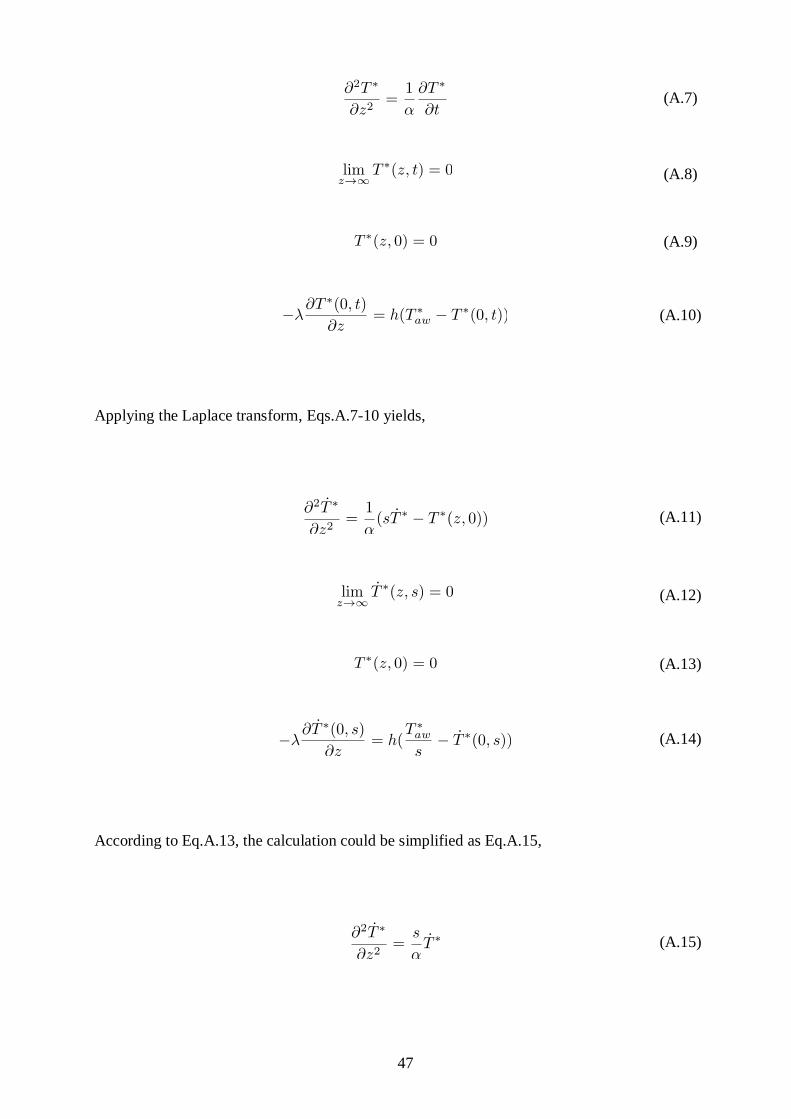
47

(A.7)

(A.8)

(A.9)

(A.10)

Applying the Laplace transform, Eqs.A.7-10 yields,

(A.11)

(A.12)

(A.13)

(A.14)

According to Eq.A.13, the calculation could be simplified as Eq.A.15,

(A.15)

48

Assume a standard solution format Eq.A.16 for , and combine it with Eq.A.14,

(A.16)

If z increased, should approach to zero according to Eq.A.12, which means that the constant B

equals zero,

(A.17)

After putting into Eq.A.14, yields a Laplace domain solution,

(A.18)

(A.19)

Using the inversed Laplace transform in (Carslaw and Jaeger,1959, transform 14),

(A.20)

(A.21)

(A.22)

The expression for could be inverted into time domain, and form a function of temperature

difference ratio,

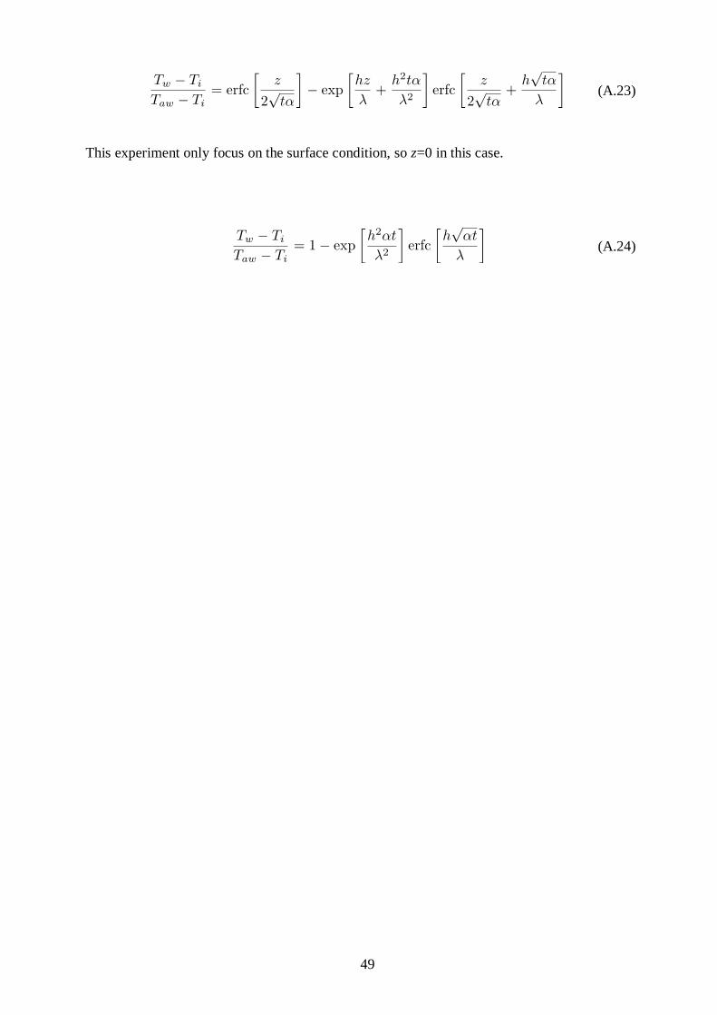
49

(A.23)

This experiment only focus on the surface condition, so z=0 in this case.

(A.24)

50

APPENDIX B: DIMENSIONAL ANALYSIS

51

APPENDIX C: PROTOCOLS

Figure 36 Type K Thermocouple Calibration Protocol

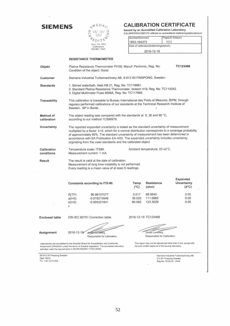
52

53

Figure 37 Pt-100 Calibration Protocol

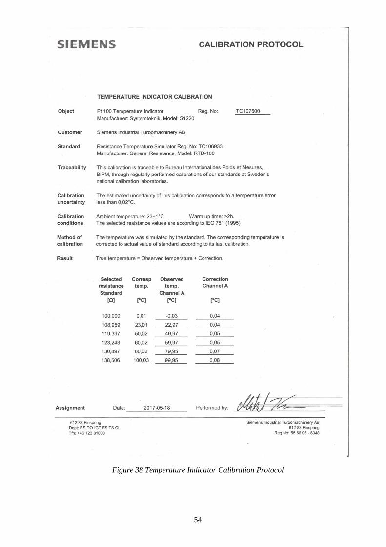
54

Figure 38 Temperature Indicator Calibration Protocol

Documents

Experimental Study of Heat Transfer Coefficient and Film