Experimental Study of Helical Shape Memory Alloy Actuators

Metals 2013, 3, 123-149; doi:10.3390/met3010123

metals ISSN 2075-4701

www.mdpi.com/journal/metals/

Article

Experimental Study of Helical Shape Memory Alloy Actuators: Effects of Design and Operating Parameters on Thermal Transients and Stroke

Shane J. Yates and Alexander L. Kalamkarov *

Department of Mechanical Engineering, Dalhousie University, PO Box 15000, Halifax, Nova Scotia,

B3H 4R2, Canada; E-Mail: [email protected]

* Author to whom correspondence should be addressed; E-Mail: [email protected];

Tel.: +1-902-494-6072; Fax: +1-902-423-6711.

Received: 22 December 2012; in revised form: 3 February 2013 / Accepted: 5 February 2013 /

Published: 18 February 2013

Abstract: Shape memory alloy actuators’ strokes can be increased at the expense of

recovery force via heat treatment to form compressed springs in their heat-activated,

austenitic state. Although there are models to explain their behaviour, few investigations

present experimental results for support or validation. The aim of the present paper is to

determine via experimentation how certain parameters affect a helical shape memory alloy

actuator’s outputs: its transformation times and stroke. These parameters include wire

diameter, spring diameter, transition temperature, number of active turns, bias force and

direct current magnitude. Six investigations were performed: one for each parameter

manipulation. For repeatability and to observe thermo-mechanical training effects, the

springs were cyclically activated. The resultant patterns were compared with results

predicted from one-dimensional models to elucidate the findings. Generally, it was

observed that the transformation times and strokes converged at changing stress levels; the

convergence is likely the peak where the summation of elastic stroke and transformation

stroke has reached its maximum. During cyclic loading, the actuators’ strokes decreased to

a converged value, particularly at larger internal stresses; training should therefore be

performed prior to the actuator’s implementation for continual use applications.

Keywords: shape memory alloys; helical shape memory alloy actuators; reaction times;

strokes; electrical resistive heating; cyclic loading

OPEN ACCESS

Metals 2013, 3 124

1. Introduction

Shape memory alloys (SMAs) got their name from their intrinsic ability to remember their shape.

Using heat treatment techniques, a SMA actuator can be programmed to be a specific shape in its heat

activated austenite phase; some shapes are more useful than others to perform mechanical work.

Popular shapes used for mechanical mechanisms include wires, bars, torsion springs, helical springs

and, more recently, wave springs [1]. SMAs in wire form are most popular, as they are readily

available, low cost and generally less difficult to model. SMA wires also provide the highest recovery

force, but unfortunately, have a low stroke; the recovery strain is typically less than 5%. The limited

stroke can be improved by using mechanical amplification mechanisms, such as levers or adjusting

curvature, as was done in Phillip Beezley’s Hylozoic Ground [2], but the mechanisms may require

significant space along with a sacrifice in recovery force. Additionally, even with mechanical

amplification, a great length of wire is needed for adequate stroke magnitudes. Sufficient space must

therefore be provided for both the length of wire and the amplification mechanism.

One option to amplify the stroke is to shape a set SMA wire into compressed helical springs. These

springs can be made using straight wire with heat treatment techniques and do not require any

amplification mechanisms, but as the internal stress is caused via torsional loading rather than axial

loading, the stress is concentrated at the wire’s perimeter, rather than being evenly distributed along

the wire’s cross-section. The recovery force decreases as a result. Furthermore, the dynamic response

and energy efficiency is worsened, mainly due to the power exploitation, under torsional loading, of

the material in the center of the solid section, which adds to the cooling time and to the power

consumption without contributing to the strength [3]. Despite their drawbacks, helical SMA actuators

have been shown to be reliable mechanical actuators, provided that the load is not substantial.

Although there have been numerous studies on the dynamic response of helical SMA actuators

(see [4–15]), their mechanical behaviour is yet to be completely understood. Additionally, most of

these studies involve using as-drawn SMA wire to be heat treated into a spring; as-drawn SMA wire is

not as readily available than annealed SMA wire and is generally more costly. Unlike as-drawn SMA

wire, annealed SMA wire has already been through the final annealing process. Putting the wire

through another annealing process could permit further diffusion and/or precipitation of Ni and Ti

atoms to form precipitates, such as Ni14Ti11 at intermediate annealing temperatures (around 450 °C) or

Ni3Ti2 at higher temperatures (around 575 °C) [16]. In both cases, the transition temperatures can

increase due to the overall decrease in nickel atomic percentage [16,17]. Moreover, putting an alloy

through an additional annealing process could lead to an increased permanent set, as well as a decrease

in ultimate tensile stress, upper plateau stress and lower plateau stress [16–18]: undesirable properties

for maximizing stroke and recovery force. Despite the warnings from the literature, annealed SMA

wires were shape set into a compressed helical spring (i.e., springs with an initial pitch angle of

approximately 0°) and were successfully installed on a reactive stage set to move textile flaps (see [19]

and [20]). Testing the shape-set helical SMA actuators at different parameters for the stage set revealed

that several parameters affected their reaction. Said revelations included a larger recovery force for

smaller spring diameters, longer cooling and heating times for larger wire diameters and that a

sufficient force is needed to extend the spring when cooled, but if too large, the spring failed to

compress when heated.

Metals 2013, 3 125

Although there are dynamic models in the literature to explain a helical SMA actuator’s behaviour,

there are few publications that present experimental results with these models for validation.

Additionally, studies with experimental support generally do not stress the material past its upper

plateau stress (such as [14] and [21]), as stress-induced martensite (SIM) would be prone to form, thus

adding further complexity to predictive models. Although limiting the maximum shear stress to its

elastic region is simpler to model and would enhance the actuator’s fatigue life, the actuator’s stroke is

limited to the change in modulus of rigidity between phase transformations; the actuator would not

transform from the de-twinning of martensite, a feature that could add up to 5% transformation strain.

Although one can use hard stops to prevent a SMA spring from reaching its upper plateau stress [22],

they are additional components that may interfere with the actuator’s dynamics; this component would

not be necessary if SMA spring mechanics were completely understood.

The aim of the present study is to determine via experimentation how certain parameters affect a

helical SMA actuator’s performance. There are three main objectives in this investigation. The first is

to find correlations between the parameters of a helical SMA actuator and its resultant dynamic

response. As mentioned, models exist to predict their behaviour, but this investigation does not aim to

validate or discredit these models for the following reasons:

• Some of the necessary material properties, such as recoverable shear strain, stress influence

coefficients and upper plateau stress were not available from the manufacturer.

• The additional heat treatment may have altered some of the material properties, including the

plateau stresses, permanent set and transition temperatures.

• The spring diameters were not measured during the transformations; one, therefore, cannot

determine the true effective diameter when the actuator is fully extended when cooled.

This investigation focused on how the helical SMAs performance—namely the actuator’s heating

time, cooling time and stroke—are affected by certain parameters. These parameters include geometry

parameters, such as the wire diameter, spring diameter and number of active turns; input parameters,

such as the direct current and bias force magnitudes; and a parameter exclusive to SMAs—the

transition temperature. Although deriving accurate models was outside the scope of this investigation,

simplified behavioural models were used in this investigation to elucidate the findings and make sense

of the experimental results. For the reaction times, the simplified models were derived using heat

transfer equations retrofitted with SMA theory. For the strokes, four models were found in

the literature.

The literature has shown that SMAs can undergo permanent deformation when thermally actuated

over multiple cycles, especially when stressed past their upper plateau stress [12,18,23]. As a second

objective, the study also investigated how each actuator’s strokes and reaction times are affected under

cyclic thermal loading. Research has shown that the transformation strain is greatest during the first

transformation and gradually decreases to a constant transformation strain after a sufficient amount of

thermal cycles [12,18,23]. Studies have shown that in SMA actuators for multiple use, lower

transformation strains (i.e., lower loads) are more desirable, as they increase fatigue life and decrease

plastic strain [12,23]. This study investigated the effects of cyclic loading to determine if similar

patterns occurred.

Metals 2013, 3 126

The third objective in this investigation is to simply catalogue the stroke and reaction times at

different spring parameters. The catalogue can be used for reference in future projects that require

specific stroke and reaction times.

2. Helical SMA Actuator Behaviour and Dynamic Outputs

As discussed, obtaining accurate models to characterize the experimental results was outside the

scope of this study. However, behavioural models were found or derived to elucidate the findings.

These models are presented in this section.

2.1. Reaction Times

If the SMA is in wire form, electrical activation is highly favoured, as it can be directly controlled,

is instantaneous and relatively simple to implement. The electric current can be direct, alternating or

pulse-width modulated. Direct current was used to activate the SMA springs in this investigation.

Using electrically resistive heat transfer relationships of a cylindrical medium with constant electrical

resistance, the elapsed time for an electrically resistive wire to heat from an initial temperature, T1, to

final temperature, T2, may be modeled as Equation 1, which was derived using the heat transfer

theorem [19]. ρ, c, d and Re', respectively, represent a conductive wire’s density, specific heat capacity,

wire diameter and resistance per unit length, while h, I and T∞, respectively, represent the convection

coefficient, direct current magnitude and ambient temperature:

∆ = −ρ4ℎ − ′π ℎ +− ′π ℎ + (1)

A SMA goes through a phase change during a transformation: a phenomenon that not only absorbs

or releases energy, but can also change its specific heat capacity and electrical resistivity. Reynaerts

and Van Brussel [24] argued that the averaged specific heat capacity during a transformation would be

the averaged value of the martensite specific heat capacity, cM, and austenite specific heat capacity, cA,

plus the transformation enthalpy divided by the temperature interval for the respective

transformation. The specific heat capacities for the martensite-to-austenite (MA) transformation, cMA,

and austenite-to-martensite (AM) transformation, cAM, could therefore be modeled as Equations 2 and

3, respectively, where XMA and XAM represent the heat absorbed during the MA and AM

transformations, respectively: = +2 + − (2)

= +2 + − (3)

As the MA and AM transformations are endothermic and exothermic, respectively, XMA and XAM,

respectively, have positive and negative values. As and Af, respectively, represent the temperatures at

which the MA transformation begins and finishes; Ms and Mf, respectively, represent the temperatures

Metals 2013, 3 127

at which the AM transformation begins and finishes. By substituting Equation 2 or 3 into

Equation 1 and assuming an electrical resistivity that is averaged between the martensite and austenite

electrical resistivities (i.e., ρM and ρA, respectively), one may solve for the transformation’s reaction

time. For a MA transformation, where T1 = As and T2 = Af, the time interval, ΔtMA, may be

presented as:

∆ = −(ρ + ρ )8ℎ − ′π ℎ +− ′π ℎ + (4)

For the AM transformation, where T1 = Ms, T2 = Mf and I = 0, the time interval, ΔtAM, may be

presented as: ∆ = −(ρ + ρ )8ℎ ln −− (5)

It must be noted that Equations 4 and 5 assume there is no stress load; the equations, therefore,

disregard any superelastic effects. When stress is applied to a SMA, the transformation temperatures

linearly increase. In the event that the alloy is subjected to a stress load, the stress-induced transition

temperatures need to be calculated and substituted into Equations 4 and 5. Performing the

substitutions, when the SMA is subjected to an axial stress load, σ, the resultant time intervals when

accounting for superelasticity may be modeled as the first portion of Equations 6 and 7, where CM and

CA represent the martensite and austenite stress influence coefficients, respectively:

∆ , = −ρ4ℎ ln + σ − ′π ℎ ++ σ − ′π ℎ + (6)

∆ , = ∆ , = −ρ4ℎ + σ −+ σ − (7)

Equations 6 and 7 would be generally applicable to straight SMA wire, however, SMA springs have

different stress distributions. At low deflections, the shear stress is due to direct and torsional shear, but

predominantly torsional shear. Additionally, when SIM forms during its austenite phase or when

martensitic de-twinning occurs, an SMA spring’s internal stress has been shown to be

non-linear [13,14,22,25], as opposed to the linear torsional shear stress observed in isotropic springs.

Although Liang and Rogers developed a constitutive model for a spring that substituted the applied

axial stress with the von Mises criterion under pure shear, i.e., σ = τ√3 [7], this cannot be directly

substituted into Equations 6 and 7, as the internal stress is not constant throughout the SMA wire. It

should also be noted that Equations 6 and 7 do not take into account the work performed by the spring

during a transformation. Regardless, Equations 6 and 7 show that internal stress does affect the SMAs

transformation times and will be used to elucidate the experimental results.

Metals 2013, 3 128

2.2. Stroke

During the study’s preparation, several one-dimensional models were found in the literature to

predict a SMA spring’s stroke. Although none would be directly compared to the experimental results,

as none effectively modeled the change in spring diameter and pitch angle, each model provided

insight to elucidating the experimental findings.

2.2.1. Elastic Stroke Model

Using traditional spring mechanics and solely accounting for the change in modulus of rigidity, the

elastic stroke model predicts a stroke, ΔδMA, equivalent to the difference between the martensite and

austenite deflections, δM and δA: ∆δ = δ − δ = 8 1 − 1 = 8 ( − ) (8)

where F, Dm, N, GM and GA represent the bias force, spring diameter, number of active turns,

martensite modulus of rigidity and austenite modulus of rigidity, respectively. Although some articles,

such as [26], state that Equation 8 can be used to calculate the overall stroke, it is generally disputed in

the literature, as it disregards the de-twinning of martensite when cooled. Although fair to assume to be

negligible, Equation 8 also fails to account for thermal strains. However, providing that the

deformation is small enough to not affect the actuator’s spring diameter and that the applied stress is

below the critical stress needed to de-twin martensite, Equation 8 may be used to model the

actuator’s stroke.

2.2.2. Constitutive Model

Unlike straight wire, helical springs are usually modeled with reference to their internal shear stress,

τ, and shear strain, γ. Based on the multidimensional constitutive relations, Liang & Rogers presented

the differential and integrated constitutive equations of a nitinol spring as Equations 9 and 10; the

equations are based on the von Mises criterion of a body experiencing pure shear [7]. As shown in

Equation 11, G represents the SMAs elastic shear modulus, which is an interpolation of the austenitic

and martensite moduli of rigidity with respect to the martensite volume fraction, ξ: dτ = dγ + Ω√3 dξ + Θ√3 d (9)τ − τ = (γ − γ ) + Ω√3 (ξ − ξ ) + Θ√3 ( − ) (10)= + ξ( − ) = 2 1 + ν + ξ(ν − ν ) (11)

The three tensors in Equations 9–11, D, θ and Ω, are known as the stiffness, thermoelastic and

transformation tensors, respectively. The stiffness and thermoelastic tensors are derived from

traditional mechanics using the associated moduli of elasticity, coefficients of thermal expansion and

martensite volume fraction. The transformation tensor is unique to SMAs. The transformation tensor

accounts for the change in strain experienced during a phase transformation and how it affects the

Metals 2013, 3 129

stress experienced by the SMA. The transformation tensor is modeled as Equation 12, where Hcur(σ) is

the maximum transformation strain at a specific stress: Ω = − (σ) (12)

Rearranging Equation 10 with initial conditions of stress, strain and martensite fraction to be 0 and

assuming Wahl concentrations to be negligible, one can solve for the spring’s maximum shear strain,

γmax, which occurs at the perimeter of the wire’s cross-section: γ = τ − Ω√3 ξ − Θ√3 (13)

Solving for the spring deflection, δ, that experiences a shear strain of γmax: δ = π = π τ − Ω√3 ξ − Θ√3 = π 8 π − Ω√3 ξ − Θ√3 (14)

Assuming a complete transformation with a negligible thermal stroke, the total stroke from a MA

transformation, ΔδMA, may be modeled as: ∆δ = π 8π − + 2(1 + υ) (σ)√3 (15)

The total stroke is thus dependent on two terms: the elastic stroke (the left term in Equation 15) and

the recovery stroke (the right term in Equation 15). Both terms add to the deflection, thus making the

overall deflection larger than the elastic stroke term alone. However, the model does not take into

account the decrease in spring diameter at large spring deformations nor permanent deformation if

strained past the alloy’s upper plateau stress.

2.2.3. Effective Stroke Model

All of the stroke formulas presented thus far assume that the spring diameter does not change

during a phase transformation. This assumption is not realistic, as the de-twinning of martensite will

encourage the spring diameter to decrease during an AM transformation. Kim et al. addressed this

issue by presenting an effective stroke model [14]: ∆δ = δ + δ + δ = πγ + 8 − 8 (16)

where δd represents the deflection from de-twinning the martensite, δL represents the elastic deflection

of the de-twinned martensite and δA represents the spring’s elastic deflection during its austenite phase.

For the δd deflection term, γd represents the shear strain experienced by the spring during the

de-twinning of martensite and is equivalent to the right most term in Equation 15. For the δL deflection

term, Deff represents the effective spring diameter after it has been reduced by the

de-twinning of martensite. However, Equation 16 fails to take account of the change in spring diameter

during the de-twinning of martensite. In addition, Kim et al. went on to model the effective

diameter as: = cos α (17)

where α represents the pitch angle. The relationship dictated by Equation 17 assumes a relatively small

pitch angle, where the spring’s vertical contour resembles a zigzag. At larger pitch angles (and

strokes), the spring’s outline becomes more sinusoidal in appearance, and the effective diameter can no

longer be determined by the pitch angle alone. Equation 16 also fails to take into account the bending

moment that becomes apparent at larger deformations and pitch angles.

Metals 2013, 3 130

2.2.4. Static Two-State Model

To account for the bending moment at larger strokes, An et al. devised a “static two-state

model” [6]. As part of the static two-state model, the total stroke was modeled as: δ = 8 + γ ξ cos α cos α cos α + sin α (1 + ν ) (18)

where γL, DA, Dγ, ξST, αi and αf represent maximum recoverable shear strain, the spring diameter in the

austenite phase, the spring diameter once the maximum recoverable shear strain has been realized, the

de-twinned martensite volume fraction, the pitch angle once the maximum recoverable shear strain has

been realized and the final pitch diameter. Although this model takes account of bending stresses only

seen in larger deformations, like the effective stroke model developed by Kim et al., the static

two-state model does not take into account the change in diameter during the de-twinning of

martensite. Likewise, the static two-state model assumes a relatively small change in pitch angle so

that the spring’s vertical contour resembles a zigzag pattern, as opposed to the sinusoidal pattern that is

observed at larger deformations. Although An et al. performed an experimental trial to validate their

static two-state model, they did not strain the spring past its maximum recoverable shear strain to avoid

permanent deformation. The model is, therefore, limited to its maximum recoverable shear strain.

3. Experimental Analysis

For repeatability, at least three trials (one trial being one individual spring) were performed for each

investigation, and every SMA spring was activated on and off for 20 cycles. Only one variable would

be manipulated at one time, while the remaining variables would be controlled. Each experiment was

set up to be compared in relation to a helical SMA actuator with a 0.25 mm wire diameter, a 3.175 mm

spring diameter, a 70 °C transition temperature and 16 active spring turns carrying a bias mass of 30 g

and activated with a 0.55 A direct current. This experimental plan was chosen to enable one to observe

how differing a single variable affects the actuator’s dynamic output.

A summary of the manipulated and controlled properties for all 6 experiments is presented as

Table 1, where each vertical column in the “Manipulated Variable Experiments” section represents one

investigation. The manipulated variable is each investigation’s title, and the magnitudes of the

manipulated variable are presented where the manipulated variable and parameter values meet; the

controlled values for the remaining parameters are listed in the remaining rows. For example, for the

wire diameter manipulation, wire diameters of 0.15 mm, 0.20 mm, 0.25 mm and 0.38 mm were

investigated with an inner spring diameter of 3.175 mm, an austenite starting temperature of 70 °C,

16 active turns, bias masses of 30 g (i.e., bias forces of 0.294 N) and direct currents of 0.55 A. With at

least three trials for each wire diameter, a minimum of 12 total springs were tested in this investigation.

Before carrying out the experiments, the heating and cooling reaction times were calculated using

Equations 4 and 5. To see if an improvement on the reaction times could be obtained when accounting

for superelasticity, the heat and cooling reaction times were also calculated using

Equations 6 and 7, substituting σ with τmax√3. These calculations were only performed to provide a

pattern of heating times and cooling times with respect to an increasing manipulated variable

parameter to elucidate the experimental findings. The convection coefficient and ambient room

Metals 2013, 3 131

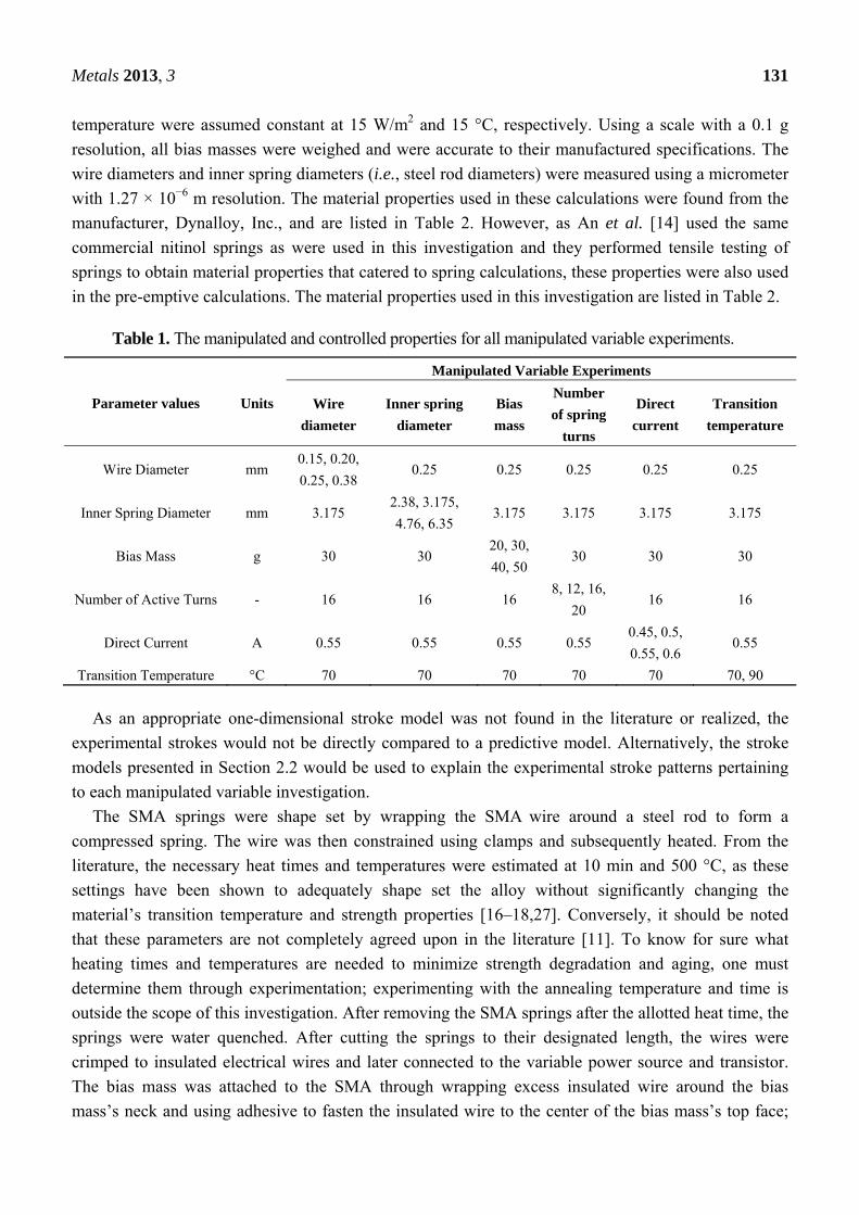
temperature were assumed constant at 15 W/m2 and 15 °C, respectively. Using a scale with a 0.1 g

resolution, all bias masses were weighed and were accurate to their manufactured specifications. The

wire diameters and inner spring diameters (i.e., steel rod diameters) were measured using a micrometer

with 1.27 × 10−6 m resolution. The material properties used in these calculations were found from the

manufacturer, Dynalloy, Inc., and are listed in Table 2. However, as An et al. [14] used the same

commercial nitinol springs as were used in this investigation and they performed tensile testing of

springs to obtain material properties that catered to spring calculations, these properties were also used

in the pre-emptive calculations. The material properties used in this investigation are listed in Table 2.

Table 1. The manipulated and controlled properties for all manipulated variable experiments.

Parameter values Units

Manipulated Variable Experiments

Wire

diameter

Inner spring

diameter

Bias

mass

Number

of spring

turns

Direct

current

Transition

temperature

Wire Diameter mm 0.15, 0.20,

0.25, 0.38 0.25 0.25 0.25 0.25 0.25

Inner Spring Diameter mm 3.175 2.38, 3.175,

4.76, 6.35 3.175 3.175 3.175 3.175

Bias Mass g 30 30 20, 30,

40, 50 30 30 30

Number of Active Turns - 16 16 16 8, 12, 16,

20 16 16

Direct Current A 0.55 0.55 0.55 0.55 0.45, 0.5,

0.55, 0.6 0.55

Transition Temperature °C 70 70 70 70 70 70, 90

As an appropriate one-dimensional stroke model was not found in the literature or realized, the

experimental strokes would not be directly compared to a predictive model. Alternatively, the stroke

models presented in Section 2.2 would be used to explain the experimental stroke patterns pertaining

to each manipulated variable investigation.

The SMA springs were shape set by wrapping the SMA wire around a steel rod to form a

compressed spring. The wire was then constrained using clamps and subsequently heated. From the

literature, the necessary heat times and temperatures were estimated at 10 min and 500 °C, as these

settings have been shown to adequately shape set the alloy without significantly changing the

material’s transition temperature and strength properties [16–18,27]. Conversely, it should be noted

that these parameters are not completely agreed upon in the literature [11]. To know for sure what

heating times and temperatures are needed to minimize strength degradation and aging, one must

determine them through experimentation; experimenting with the annealing temperature and time is

outside the scope of this investigation. After removing the SMA springs after the allotted heat time, the

springs were water quenched. After cutting the springs to their designated length, the wires were

crimped to insulated electrical wires and later connected to the variable power source and transistor.

The bias mass was attached to the SMA through wrapping excess insulated wire around the bias

mass’s neck and using adhesive to fasten the insulated wire to the center of the bias mass’s top face;

Metals 2013, 3 132

this ensured that the corresponding end of the insulated wire along with the bias mass were in line with

the SMA spring to minimize connection eccentricities and resultant stress concentrations. It should be

noted, however, that eccentricity was not entirely avoided, as the insulated wires were directly crimped

to the SMA spring.

Table 2. The material properties of the shape memory alloy (SMA) wire and estimated

material properties.

Figure 1 gives a sketch of the SMA spring/bias mass apparatus along with its main geometrical

parameters. The overall testing apparatus is pictured in Figure 2, while Figure 3 gives a close-up of the

electronic components (for an electronic schematic of the apparatus, refer to [19]). The apparatus was

controlled using an Arduino duemilanove (2009) microprocessor. The power source had variable

current settings, allowing the SMA wire to be activated using direct current of a constant magnitude.

The direct current was turned on and off using the microprocessor and a transistor. To sense the

position of the bias mass, an ultrasonic ranger was used. The code was written to detect when the bias

mass was stationary, i.e., when a transformation has ended. When the microprocessor detected a

stationary bias mass, its input to the transistor switched from high to low or vice versa. Originally, the

ultrasonic ranger was meant to measure the austenite lengths, martensite lengths and strokes; however,

Property Value Source

Density, ρ 6.45 g/cm3 [28]

Specific Heat, cA = cM 837.36 J/kg/K (0.2 cal/g*°C) [28]

Latent Heat of Transformation, X 24,190.4 J/kg (5.78 cal/g) [28]

Electrical Resistivity

Austenite, ρA

Martensite, ρM

100 micro-ohms*cm

80 micro-ohms*cm [28]

Transition Temperatures

As

Af

Ms

Mf

70°C Wire 90 °C Wire

[28]

70 90

90 110

65 80

45 60

Modulus of Elasticity

Martensite, EM

Austenite, EA

28 GPa

83 GPa

[28]

Poisson’s Ratio, ν (Estimated from

the literature) 0.3 [23]

Stress Influence Coefficients (Estimated

from the literature)

CA

CM

7 MPa/°C

7 MPa/°C

[23]

Critical Shear Stresses

Start of Martensite De-twinning, τ 114.0 MPa [14]

End of Martensite De-twinning, τ 72.4 MPa [14]

Upper Plateau Shear Stress, τ 183 MPa [14]

Maximum Recoverable Shear Strain, γL 0.05 [14]

Metals 2013, 3 133

the ultrasonic ranger tended to underestimate the strokes by up to 10 mm. The austenite lengths,

martensite lengths and strokes were therefore measured by the operator using a stationary ruler. The

times between transitions (i.e., the reaction times) were measured and recorded by the microprocessor.

Figure 1. Sketch of the SMA spring setup, including dimensions and components. The

sketched spring has nine active coils and one dead coil. Dimensions include the wire

diameter (d), inner spring diameter (Di), mid spring diameter (Dm) and outer spring

diameter (D0).

DoDmDi

d

Active Coils

Bias Mass

Dead Coil

Crimp

Crimp

DeadCoil

Connection toTransistor's Collector

Connection toPositive VoltageSource

Figure 2. The labelled testing apparatus for the SMA helical spring experiments.

Ultrasonic Ranger

Metals 2013, 3 134

Figure 3. A close-up of the testing apparatus’s electronic components.

During a trial, the Arduino code was activated. The transistor’s base was initially turned high,

allowing direct current to activate a MA transformation in a SMA spring. Taking the data from the

ultrasonic sensor, the microprocessor determined when the transformation is complete, upon which the

microprocessor turned the transistor’s base low, allowing the SMA wire to cool back to its martensite

form. The microprocessor logged the elapsed time, i.e., the heating time. When the SMA wire finished

its AM transformation as determined by the microprocessor, the transistor’s base was turned to high,

and the microprocessor logged the elapsed time, i.e., the cooling time. As mentioned, the martensite

lengths, austenite lengths and strokes were measured using a stationary ruler by the operator. Each trial

consisted of 20 cycles, giving 20 heating times, cooling times, martensite spring lengths, austenite

spring lengths and stroke measurements. 20 cycles were performed not only for repeatability, but to

also observe if the results changed after subsequent activation cycles due to training. If training is a

factor, the stroke would be expected to be highest during the first activation and decreasing after each

subsequent cycle, until the stroke converges to a set stroke.

For each trial, the mean, median and %-standard deviation were obtained. To obtain the results for

each setting as a whole, the results from the respective trials (at least three) were combined to get the

averaged mean, averaged median and %-pooled standard deviation. On some trials, a few heating and

cooling times were observably shorter than what was recorded; these trials had larger standard

deviations as a result. As these few outliers skewed the mean values, it was felt that the median values

would better reflect the true reaction times. The averaged median values were thus used for further

analysis and discussion along with the averaged values obtained from the first and last

(i.e., 20th) actuations.

4. Results and Discussion

The experimental reaction times were compared to those calculated using Equations 4 to 7 to clarify

the findings. The calculated values are presented in Table 3. For the equations accounting for

superelasticity, i.e., Equations 6 and 7, the axial stress (σ) was replaced with the von Mises equivalent

of the spring’s maximum shear stress (i.e., σ = τmax√3 = 8√3 (π )⁄ ). For the heating times,

neither Equation 4 nor Equation 6 accurately predicted the reaction times; the calculations were

generally underestimated by 70%. However, Equation 6 did project the correct correlations between

heat time and a manipulated parameter. Alternatively, for the cooling times, the calculations that

Metals 2013, 3 135

included superelastic effects better correlated to the experimental cooling times. Without accounting

for superelasticity (i.e., Equation 5) the cooling times were greatly overestimated, often having

errors greater than 100%. Alternatively, the cooling time formula that included superelasticity

(i.e., Equation 7) often had calculated cooling times that were within 10% of the experimental cooling

times. This result supports the notion that superelasticity cannot be ignored when calculating the

reaction times. However, it should be reiterated that Equation 4 through Equation 7 were generalized

equations that omitted several important parameters, including the work being done during a

transformation, the change in spring diameter and substituting the axial stress with the maximum shear

stress; the shear stress actually varies from zero at the wire’s center and non-linearly increases to its

maximum value at the wire’s perimeter. Nonetheless, these equations gave insight towards explaining

the experimental results.

Table 3. Calculated values using Equations 4–8.

Manipulate

d variable Magnitude

Calculated

heating time

without

accounting

for

superelasticit

y (i.e., Equation 4)

Calculated

heating time

accounting for

superelasticity

(i.e., Equation 6)

Calculated

cooling time

without

accounting for

superelasticity

(i.e., Equation 5)

Calculated

cooling time

accounting

for

superelasticit

y (i.e.,

Equation 7)

Calculated

stroke using

the elastic

stroke model

(i.e., Equation 8)

Wire

Diameter

0.145 mm 0.54 s 0.66 s 16.2 s 2.6 s 198 mm

0.192 mm 0.98 s 1.09 s 21.6 s 6.6 s 66 mm

0.248 mm 1.68 s 1.79 s 27.9 s 13.5 s 25 mm

0.375 mm 4.02 s 4.15 s 42.1 s 31.8 s 5.4 mm

Inner Spring

Diameter

2.38 mm 1.68 s 1.76 s 27.9 s 15.4 s 11 mm

3.175 mm 1.68 s 1.79 s 27.9 s 13.5 s 25 mm

4.76 mm 1.68 s 1.85 s 27.9 s 10.9 s 80 mm

6.35 mm 1.68 s 1.91 s 27.9 s 9.1 s 180 mm

Bias

Mass/Bias

Force

20 g/0.196 N 1.68 s 1.75 s 27.9 s 16.3 s 1.7 mm

30 g/0.294 N 1.68 s 1.79 s 27.9 s 13.5 s 2.5 mm

40 g/0.392 N 1.68 s 1.83 s 27.9 s 11.5 s 3.3 mm

50 g/0.490 N 1.68 s 1.87 s 27.9 s 10.1 s 4.2 mm

Number of

Turns

8 1.68 s 1.79 s 27.9 s 13.5 s 1.2 mm

12 1.68 s 1.79 s 27.9 s 13.5 s 1.9 mm

16 1.68 s 1.79 s 27.9 s 13.5 s 2.5 mm

20 1.68 s 1.79 s 27.9 s 13.5 s 3.1 mm

Direct

Current

0.45 A 2.63 s 2.93 s 27.9 s 13.5 s 2.5 mm

0.50 A 2.07 s 2.25 s 27.9 s 13.5 s 2.5 mm

0.55 A 1.68 s 1.79 s 27.9 s 13.5 s 2.5 mm

0.60 A 1.39 s 1.46 s 27.9 s 13.5 s 2.5 mm

Transition

Temperature

70 °C 1.68 s 1.79 s 27.9 s 13.5 s 2.5 mm

90 °C 1.64 s 1.76 s 19.6 s 10.8 s 2.5 mm

Metals 2013, 3 136

For the experimental strokes, none of the results were directly compared with any of the

one-dimensional models presented in Section 2.2, as they all had problems accounting for the change

in spring diameter at large deformations, especially with deformations that strain the SMA spring past

its maximum recoverable shear strain. To gain insight towards explaining the experimental results, the

elastic stroke model (i.e., Equation 8) was used to calculate what the stroke would be if one only took

account of the change in modulus of elasticity. These calculated elastic strokes are presented in

Table 3. One continuing trend that occurred throughout the investigations was a convergence to a

specific stroke value. This convergence was observed in manipulations that changed the internal stress,

i.e., the bias force, wire diameter and spring diameter manipulations. It is believed that the

convergence is actually a peak where the summation of the strokes due to martensitic de-twinning and

change in modulus of rigidity has reached its maximum.

When comparing the averaged first, median and end strokes from each trial set, the averaged first

strokes recorded during the first cycle were generally larger than the averaged median and end strokes.

Additionally, the strokes recorded during the last cycle were generally the shortest among the three

values. These observations are consistent with training and cyclic effects observed in literature. For

continuous, reliable strokes, an SMA spring actuator should, therefore, undergo cyclic loading prior to

its implementation. With regards to the heating and cooling times, the first, median and end cycles did

not tend to deviate from each other in a consistent pattern.

Divided further into seven subsections, one for each variable and a discussion on the internal stress

and the deformation strain, this section presents and discusses the investigation’s results.

4.1. Wire Diameter

Table 4 presents the wire diameter manipulation’s results with respect to the averaged first, median

and last value for each wire diameter. Figure 4a plots the wire diameter manipulation’s averaged

median heat and cooling times, while Figure 4b plots the averaged strokes, martensite lengths and

austenite lengths. Based on the heat and cooling time calculations performed using Equation 6 and 7,

both reaction times were expected to increase in relation to an increased wire diameter, as the increase

in volume leads to an increased thermal heat capacity; the experimental results generally supported this

correlation. The first cycle generally produced the larger heat and cooling times, followed by the

median and final cycles, but this pattern was not consistent for all wire diameter manipulations. It is

therefore difficult to know if cycling had an effect on the reaction times.

Table 4. The averaged first, median and last values for the wire diameter manipulation.

Wire

diameter

(mm)

Heat time (s) Cooling time (s) Martensite length

(mm)

Austenite length

(mm) Stroke (mm)

First Med. Last First Med. Last First Med. Last First Med. Last First Med. Last

0.145 4.3 2.8 2.3 3.2 3.1 3.3 178 178 177 134 145 147 44 33 30

0.192 3.6 3.3 3.4 7.5 6.9 6.2 167 168 169 59 71 77 109 96 92

0.248 6.9 6.3 7.1 11.9 12.7 11.3 128 132 129 28 30 30 100 102 99

0.375 8.4 7.8 7.9 15.2 14.8 14.1 151 158 163 44 55 62 107 102 101

Metals 2013, 3 137

Figure 4. Experimental results from the wire diameter manipulation. (a) (Left) The

averaged median heat and cooling times. (b) (Right) The averaged median strokes,

martensite lengths and austenite lengths.

(a) (b)

With regards to the stroke, had the change in moduli of rigidity been the only factor between phase

transitions, the stroke would decrease with respect to an increasing diameter; this was not observed in

the experimental results. When increasing the wire diameter from 0.145 mm to 0.192 mm, the stroke

nearly tripled from 33 mm to 96 mm before converging to a set stroke of 102 mm at subsequent wire

diameter increases. The low stroke for the 0.15 mm wire diameter can be explained from its internal

stress; ignoring the change in spring diameter, the maximum shear stress is estimated at a value of

823 MPa: more than four-times the upper plateau stress found by An et al. [14]. The 0.145 mm wire

diameter spring is thus forced to go beyond its recoverable shear strain limit, causing permanent

deformation. The convergence to 102 mm could suggest that there is a limit to the amount of stroke

that can be obtained for a helical SMA with respect to an increasing wire diameter. Alternatively, the

converged value may actually be the peak of a plateau where the stroke may decrease at further wire

diameter increases. As the wire diameter increases, the SMA spring’s internal shear stress decreases,

which could limit the amount of martensite that can be de-twinned by the bias force and, consequently,

limit the stroke. Adding to the notion that permanent deformation occurred in the 0.15 mm to 0.20 mm

wire diameter springs is the change in austenite length over subsequent cycles. Had no permanent

deformation occurred, one would expect the austenite lengths to remain relatively constant throughout

cycling. With the exception of the 0.25 wire diameter springs, there were observed increases in

austenite lengths during cycling. Permanent strain was expected on the 0.15 mm and 0.20 mm wire

diameters, as the estimated maximum internal shear stresses were 823 MPa and 355 MPa, which are

both well above the alloy’s projected upper plateau stress of 183 MPa, but permanent strain was not

expected for the 0.38 mm spring.

The increase in martensite and austenite lengths when comparing the 0.25 mm to 0.38 mm wire

diameters was an interesting result. The austenite length was expected to further decrease for the

associated increase in wire diameter as the estimated maximum shear stress decreased from 167 MPa

to 50.4 MPa. Decreasing to an internal stress below the τ estimated by An et al. [14] should therefore

not inhibit the transformation from taking place and not cause any permanent elastic strain in its

austenite phase. As the 0.38 mm springs’ austenite lengths did increase after subsequent cycles, plastic

Metals 2013, 3 138

deformation had occurred. An explanation for this may lie in the SMA spring’s preparation. When

preparing the 0.38 mm wire diameter SMA spring, an increased amount of mechanical resistance was

noticed when wrapping the annealed SMA wire around the steel rod. The other smaller wire diameters

did not have this mechanical resistance, likely due to the fact that the wires were sufficiently small to

solely deform via martensitic de-twinning. It is conceivable that the 0.38 mm spring may have

surpassed its transformation strain when wrapped around the steel rod and, thus, may have further

deformed via plastic deformation. This could explain the jump in austenite and martensite spring

lengths. Remarkably, the jump in austenite spring length did not appear to influence the transformation

stroke, as the martensite deflection accordingly increased to maintain the converged median stroke

value of 102 mm.

4.2. Spring Diameter

Table 5 presents the spring diameter manipulation’s results with respect to the averaged first,

median and last values obtained for each spring diameter. Figure 5a plots the spring diameter

manipulation’s averaged median heat and cooling times, while Figure 5b plots the averaged median

strokes, martensite lengths and austenite lengths.

Table 5. The averaged first, median and last values for the spring diameter manipulation.

Inner

spring

diameter

(mm)


(mm)

Austenite length

(mm) Stroke (mm)


2.38 5.4 5.1 5.0 17.0 16.1 16.3 75 75 78 16 17 18 67 58 59

3.175 6.9 6.3 7.1 11.9 12.7 11.3 128 132 129 28 30 30 100 102 99

4.76 10.9 9.5 10.7 9.7 8.5 10.6 233 234 236 78 81 83 159 152 149

6.35 10.3 9.3 8.6 9.0 10.6 10.6 314 318 319 146 159 167 173 158 151

Figure 5. Experimental results from the spring diameter manipulation. (a) (Left) The

averaged heat and cooling times. (b) (Right) The averaged strokes, martensite lengths and

austenite lengths.

(a) (b)

Metals 2013, 3 139

For the reaction times, Equations 6 and 7 projected that the heat times and cooling times would

respectively increase and decrease with an increasing spring diameter. Larger spring diameters have a

larger internal stress; larger stresses in turn cause the transition temperatures to increase. More time is

thus needed to reach the MA transition temperatures during heating, while less time is needed to reach

the AM transition temperatures during cooling. This projection was observed in the experimental

results. The smallest spring diameter spring (2.34 mm inner diameter) had the shortest averaged

median heat time of 5.1 s. The averaged median heat time would increase over two subsequent spring

diameter increases before converging to a value of 9.3 s at the largest inner spring diameter of

6.36 mm. A similar converging trend was observed for the cooling times. The smallest spring diameter

had the largest averaged median cooling time of 16.1 s and decreased over two subsequent spring

diameter increases. Interestingly, however, the averaged median cooling time increased over the final

increase in spring diameter; springs with an inner spring diameter of 4.80 mm and 6.36 mm had values

of 8.5 s and 10.6 s, respectively. It is believed that permanent deformation may be responsible for this

increase in cooling time.

Regarding the strokes as plotted on Figure 5b, like the wire diameter manipulation, the stroke

increased as the inner spring diameter was increased, but converged to a set value; said value was

158 mm. Also, like the wire diameter, this convergence is likely due to the increase in internal stress.

As the inner spring diameter increased from 2.34 mm, to 3.18 mm, to 4.80 mm and to 6.36 mm, the

estimated maximum shear stress increased from 127 MPa, 167 MPa, 247 MPa and 323 MPa. The last

two spring diameters had maximum shear stresses that surpassed the alloy’s upper plateau stress of

183 MPa, as estimated by An et al. [14]; permanent strain would therefore be expected and, thus, limit

the maximum recoverable strain. Looking at the recorded cyclic effects in this investigation, the

smaller spring diameters had little change in austenite length (less than 2 mm), thus indicating that

permanent strain minimally influenced the stroke. However, the larger two spring diameters had larger

changes in austenite length; the 4.80 mm inner spring diameter had a 5 mm change in austenite length,

while the 6.36 mm had more than four times the change in austenite length, with a value of 21 mm.

These results suggest that providing the upper plateau stress is surpassed, larger stresses will further

decrease the overall stroke under cyclic loading due to permanent deformation.

With regards to the change in modulus of rigidity, the elastic stroke model projects that the stroke

would continuously increase with an increasing diameter. The results suggest that the increasing elastic

stroke and decreasing transformation stroke could be responsible for the converging stroke value; the

observed convergence is likely that of a peak value where the summation of the elastic stroke and

recoverable stroke has reached its maximum. Had larger spring diameters been investigated, the

authors stipulate that strokes would continue to decrease, as said spring diameters would have larger

internal stresses and, therefore, induce more permanent strain.

Another possible contribution to the converged values may be the decrease in spring diameter and

increase in pitch angle during the low temperature, martensite phase. From the effective stroke and

static two-state models presented in Section 2.2, a decrease in spring diameter and increase in pitch

angle would in turn decrease the overall martensite deflection and stroke.

Metals 2013, 3 140

4.3. Bias Force

Table 6 presents the bias force manipulation’s results with respect to the averaged first, median and

last value obtained for each bias force. Figure 6a plots the bias force manipulation’s averaged median

heat and cooling times, while Figure 6b plots the averaged strokes, martensite lengths and

austenite lengths.

Table 6. The averaged first, median and last values for the bias force manipulation.

Bias

Force

(N)


(mm)

Austenite length

(mm) Stroke (mm)


0.196 6.4 4.9 4.9 18.3 18.5 16.7 103 103 105 21 22 22 82 81 83

0.294 6.9 6.3 7.1 11.9 12.7 11.3 128 132 129 28 30 30 100 102 99

0.392 10.2 8.6 8.8 10.8 10.9 11.0 137 140 142 34 39 41 103 101 101

0.490 11.6 11.3 11.2 11.7 10.4 10.6 150 153 155 43 53 59 107 100 96

Figure 6. Experimental results from the bias force manipulation. (a) (Left) The averaged

heat and cooling times. (b) (Right) The averaged strokes, martensite lengths and

austenite lengths.

(a) (b)

Based on the projections from Equations 4 and 5, it was anticipated that, with respect to an

increasing bias force, the heat times and cooling times would increase and decrease, respectively. An

increased bias force would induce a greater internal shear stress and, thus, increase the wire’s transition

temperatures throughout the wire’s radius due to superelasticity. This projection was observed in the

experimental results. For springs that were biased with 0.196 N, 0.294 N, 0.392 N or 0.490 N, the

averaged heat times were 18.5 s, 12.7 s, 10.9 s and 10.4 s, respectively, while the averaged cooling

times were 4.9 s, 6.3 s, 8.6 s and 11.3 s. There were some differences in reaction times obtained in the

first, median and last cycle, but the differences were not in a consistent pattern and, thus, do not

support the notion that cycling has an effect on the reaction times.

The stroke increased from roughly 80 mm to 100 mm when the bias force increased from 0.196 N

to 0.294 N, but remained constant at around 100 mm on further bias force increases (up to 0.490 N).

Like the wire diameter and spring diameter manipulations, the stroke appears to converge to a set

Metals 2013, 3 141

value. Also, like the wire diameter and spring diameter investigations, the cause of this convergence is

likely due to the recoverable shear strain limit. At bias forces of 0.196 N, 0.294 N, 0.392 N and

0.490 N, the projected maximum internal shear stresses are 111 MPa, 167 MPa, 223 MPa and

278 MPa, respectively. Assuming that the alloy’s upper plateau stress is the value estimated by

An et al. [14], the maximum recover shear strain was surpassed for springs actuated with 0.392 N and

0.490 bias forces and, therefore, should cause permanent strain. If one looks at the cyclic changes in

austenite length for all bias forces (i.e., the difference in the averaged first and last values), one would

observe that there was relatively no change for the 0.196 N or 0.294 N bias forces (1 mm and 2 mm,

respectively), but the austenite lengths did noticeably increase for the 0.392 N and 0.490 N bias forces

(7 mm and 16 mm). This suggests that the 0.392 N and 0.490 N did indeed succumb to some plastic

deformation. Furthermore, the 0.490 N biased springs succumbed to more than twice the plastic

deformation experienced by the 0.392 N biased springs, suggesting that the plastic deformation is

greater for larger internal stresses. Additionally, the change in modulus of rigidity (i.e., the elastic

stroke model presented in Section 2.2) suggests an increasing stroke with an increasing bias force. The

combination of an increasing elastic stroke with an increase in permanent strain may be responsible for

the stroke convergence observed in this investigation.

Like the spring diameter investigation, another contribution to the stroke convergence may be the

decrease in spring diameter in the low temperature, martensite phase. At larger bias forces, the internal

stress is greater and induces the martensite diameter to decrease and better disperse the stress. As

already mentioned, the smaller martensite diameter would lead to a decreased elastic stroke, which in

turn may have contributed to the stroke’s convergence.

4.4. Number of Active Turns

Table 7 presents the number of active turns manipulation’s results with respect to the averaged first,

median and last value obtained for each turn amount. Figure 7a plots the number of active turns

manipulation’s averaged median heating and cooling times, while Figure 7b plots the averaged strokes,


Table 7. The averaged first, median and last values for the number of active

turns manipulation.

Number

of active

turns


(mm)

Austenite length

(mm) Stroke (mm)


8 6.6 6.5 6.9 12.4 10.4 10.0 73 74 75 18 18 19 58 55 55

12 6.3 6.1 6.6 14.4 13.0 12.6 105 105 107 22 24 25 84 82 81

16 6.9 6.3 7.1 11.9 12.7 11.3 128 132 129 28 30 30 100 102 99

20 6.1 6.0 6.7 11.6 12.7 13.9 168 171 175 36 38 40 143 133 131

As the number of spring turns is absent in the reaction time equations and does not influence a

spring’s internal stress, it was predicted that neither the heat times nor cooling times would change in

relation to an increasing number of spring turns; the experimental results generally agreed with this

prediction. With regards to the averaged median heat times, the values for all four spring turn values

Metals 2013, 3 142

were all within 0.5 s of each other, while three out of the four cooling times were within 0.3 s of each

other. The one exception was the smallest spring, the eight-turn spring, which had an averaged median

heat time that was 2.4 s shorter than the average of the other spring turn values. One possible

explanation for the eight-turn spring’s smaller cooling time was the smaller stroke; the control system

may have interpreted the bias mass as stationary, when in fact, the mass may still have been slowly

moving. Another possible explanation may have been a larger conductive heat sink influence at the

SMA spring’s connections. With regards to cyclic effects, the heating times were generally consistent

among the first, median and last cycles, suggesting that cycling does not affect the heat time.

Although, there was some discrepancy among first, median and last cooling times, there does not

appear to be a regular discrepancy pattern to indicate a correlation between cooling time and

cyclic effects.

Figure 7. Experimental results from the number of active turns manipulation.

(a) (Left) The averaged heat and cooling times. (b) (Right) The averaged strokes,


(a) (b)

With reference to the stroke, it was predicted that not only the stroke would increase in relation to

an increasing number of spring turns, but would linearly increase, as the number of spring turns

theoretically have no relation to the overall stress and should therefore not influence the transformation

strain. As the internal stress should be constant for all four spring turn manipulations, the

transformation strain should therefore be constant for all four spring manipulations. Likewise, as all

springs have the same bias force, wire diameter, spring diameter and moduli of rigidity, the elastic

strain should also be the same value for all four spring turns. As predicted, the experimental stroke

increased in a linear fashion. A linear regression was performed on the results with an R2 value of

0.993; a linear relationship is thus probable. With regards to cyclic effects, there appears to be little

discrepancy between the first, median and last stroke values, indicating that little or no permanent

strain was present throughout the manipulation. As the estimated shear stress of 167 MPa is less than

the 183 MPa upper plateau stress found by An et al. [14], it is conceivable that the springs did not

suffer from any permanent strain.

Metals 2013, 3 143

4.5. Direct Current

Table 8 presents the direct current manipulation’s results with respect to the averaged first, median

and last value obtained for each turn amount. Figure 8a plots the direct current manipulation’s

averaged median heat and cooling times, while Figure 8b plots the averaged strokes, martensite lengths

and austenite lengths.

Table 8. The averaged first, median and last values for the direct current manipulation.

Direct

Current

(A)


(mm)

Austenite length

(mm) Stroke (mm)


0.45 15.6 16.2 17.0 11.0 11.1 11.1 134 140 142 57 60 69 84 78 76

0.50 10.5 9.5 11.0 10.9 11.4 10.8 132 132 136 29 32 34 114 100 96

0.55 6.9 6.3 7.1 11.9 12.7 11.3 128 132 129 28 30 30 100 102 99

0.60 6.7 4.7 4.9 12.6 11.0 11.8 126 127 133 24 28 29 111 99 100

Figure 8. Experimental results from the direct current manipulation.

(a) (Left) The averaged heat and cooling times. (b) (Right) The averaged strokes,


(a) (b)

For the reaction times, with respect to an increasing direct current magnitude, it was predicted that

the heat times would decrease due to the increase of thermal energy, while the cooling times would

remain constant, as the transformation would stop at the same final temperature regardless of direct

current magnitude. Both predicted patterns were generally correct. Using the averaged median values,

the heat times comparatively decreased from 16.2 s, to 9.5 s, to 6.3 s and to 4.7 s for springs that were

actuated with direct currents of 0.45 A, 0.50 A, 0.55 A and 0.60A, respectively, while the cooling

times were all within 1–7 s of each other. Similar to the other investigations, the first, median and last

reaction times showed some discrepancy with each other, but not in a consistent pattern to suggest that

cycling affects the reaction times.

With regards to the strokes, it was anticipated that the strokes would be unaffected by a change in

direct current, providing that the current is sufficient to induce the transformation. This prediction,

Metals 2013, 3 144

overall, aligned with the experimental results, as the averaged median strokes for the springs actuated

by 0.50 A, 0.55 A or 0.60 A were within 2% of each other with values around 100 mm. However, the

0.45 A trials produced an averaged median stroke of 78 mm. This can be attributed to the control

system. During the 0.45 A trials, the bias mass often moved quite slowly during the transformation; the

control system would sometimes mistake it for being stationary. At times, when the control system

allowed a spring to fully transform at 0.45 A, the stroke would generally be around 100 mm, but the

control system would often cut the true stroke short to as low as 40 mm, because it was moving

slowly. Had the control system allowed the spring to completely transform, the true median stroke

value would likely have been around 100 mm, like the other direct current magnitudes. Although there

was some discrepancy between the first stroke and the median and last strokes for the springs activated

by 0.50A and 0.60A direct currents, this pattern was not observed throughout all direct current

magnitudes, thus not supporting that direct current influences permanent strain. As the direct current

does not affect the static stress experienced by the SMA spring, it is expected that direct current does

not influence permanent strain.

4.6. Transition Temperature

For the transition temperature manipulation, Table 9 presents the results with respect to the

averaged first, median and last value. With respect to transition temperature, Figure 9a plots the

averaged median heat and cooling times, while Figure 9b plots the averaged strokes, martensite lengths

and austenite lengths.

Table 9. The averaged first, median and last values for the springs with 90 °C austenitic

starting temperature.

As


(mm)

Austenite length

(mm) Stroke (mm)


70 °C 6.9 6.3 7.1 11.9 12.7 11.3 128 132 129 28 30 30 100 102 99

90 °C 7.9 5.8 5.9 7.3 6.4 6.4 167 175 177 70 107 118 64 67 58

Figure 9. Experimental results from the transition temperature manipulation. (a) (Left) The

averaged heat and cooling times. (b) (Right) The averaged strokes, martensite lengths and

austenite lengths.

(a) (b)

Metals 2013, 3 145

With relation to reaction times, the derived heat transfer equations projected that the heat times and

cooling times would respectively increase and decrease with an increased transition temperature; a

higher transition temperature would require more time to attain when heated and require less time to

attain when cooled. In terms of heating times, there was no observable difference between the 70 °C

and 90 °C springs; the averaged median heat times were within 9% of each other. For the cooling

times, the prediction was correct; taking approximately 50% less time, the 90 °C SMA springs

extended faster than their 70 °C counterparts. When analyzing the cyclic effects of the 90 °C SMA

springs, the heat and cooling times obtained from the first cycle were both larger than their last and

median counterparts, which were within 2% of each other. This suggests that cycling did affect the

reaction times for the 90 °C SMA springs.

It was perceived that the stroke would not change in relation to the transition temperature, as the

transition temperature is absent from any of the models presented in Section 2.2. In opposition of said

projection, the experimental results demonstrated that the transition temperature does have an

influence on the stroke. When comparing the 90 °C SMA springs to their 70 °C counterparts, the

strokes decreased by 34%. When comparing the changes in austenite length through cycling, the 90 °C

SMA springs had a 69% increase from first and last austenite lengths, while the 70 °C SMA springs

only had a 7.1% increase. Not only did the stroke decrease, but the 90 °C SMA springs suffered more

from fatigue under cyclic loading. Evidently, the 90 °C is not as strong as the 70 °C wire. This may be

due to different additives in the 90 °C wire that were added by the manufacturer to increase its

transition temperature at the expense of the SMAs strength; however, the literature shows that

additives are more likely to strengthen a material rather than weaken it [27,29]. A more plausible

explanation is that the 90 °C SMA wires were aged on purpose by the manufacturer to increase the

transition temperature. Aging will increase the transition temperature, but at the expense of its strength

properties, including its upper plateau strength [11,16,17,27]. A decreased upper plateau strength

would in turn decrease the maximum transformation strain, which correlates with the

experimental results.

4.7. Transformation Strain vs. Maximum Shear Stress

The results from the investigations suggested a correlation between stroke and internal stress. The

stress needs to be large enough to exploit the recoverable transformation stroke, i.e., the recoverable

de-twinning of martensite, but if the maximum shear stress surpasses a critical amount, permanent

strain will develop and impede the total stroke. The results suggest that a combination of elastic strain,

i.e., the change in modulus of rigidity, and the recoverable transformation strain contribute to the

overall stroke. Using the shear strain formula with respect to deflection (i.e., γ = (δ ) (π )⁄ ), the

shear strain associated with the averaged median stroke was found and plotted with reference to the

approximated maximum shear stress (i.e., τ = (8 ) (π )⁄ ) (see Figure 10). The stroke shear

strain appears to peak around the alloy’s upper plateau stress of 183 MPa [14], suggesting that the

stroke can be maximized at this critical stress value. However, the peak was not observed for the wire

diameter investigation, as the largest wire diameter of 0.38 mm produced the largest stroke strain at an

estimated maximum shear stress of 50.4 MPa. As mentioned in Section 4.1, the authors attribute this

increase in stroke to the preparation of the SMA springs with 0.38 mm wire diameter.

Metals 2013, 3 146

Figure 10. The approximate stroke shear strain vs. approximate maximum shear stress.

5. Conclusions

Recalling the first objective, it was desired to find correlations between a SMA spring’s parameters

and their dynamic response. This investigation successfully tested how six variables (i.e., wire

diameter, spring diameter, bias force, number of active spring turns, direct current magnitude and

transition temperature) independently affect the performance of SMA actuators in relation to their

reaction times and strokes. It was found that four out of six variables affect the heating time, four out

of six variables affect the cooling time and all six variables affect the stroke. These experimental

results will provide helical SMA actuator designers a better understanding of how each parameter

affects the actuator’s resultant reaction times and strokes. Recalling the second objective, the study

also aimed to observe how cycling affects a helical spring’s reaction times and strokes.

Throughout this investigation, there have been some common behavioural patterns among a helical

spring’s mechanical output. For the heat times (i.e., elapsed time for a MA transformation), it was

found that the patterns projected by the derived heat transfer equation that accounted for superelasticity

(Equation 6) were generally correct (the exception being the transition temperature investigation), but

greatly underestimated the true heat times. This was expected, as the equation does not take into

account the work being exercised by the helical SMA actuator. However, for the cooling times (i.e.,

the elapsed time for an AM transformation), the patterns projected by the derived heat transfer

equation (Equation 7) were not only generally correct, but most values were within 10% of the

experimental values, indicating that it can provide a good estimate of the true reaction time. However,

it is reiterated that the derived equation is generalized, and some properties used in the calculations

were estimated, not found. Nonetheless, the overall results support that superelasticity cannot be

overlooked when predicting a helical SMAs reaction times. Overall, cycling did not show any

consistent changes in heat times or cooling times. Although there was variation in reaction times

regarding the first, median and last values, the variation was not consistent to suggest that cycling

alters the reaction times. The only investigation that did show consistent variation was the transition

temperature investigation; it is speculated that this occurred due to the different material properties of

the 90 °C SMA wire.

The investigation supported that internal stress influences the stroke. For the investigations that

involved increases or decreases in shear stress; i.e., the wire diameter, spring diameter and bias force

Metals 2013, 3 147

investigations; a common theme of stroke convergence was observed. Based on permanent strain as

observed by cyclic changes in austenite lengths, it is stipulated that this convergence is actually a peak,

where the combined effects of modulus of rigidity change and martensitic de-twinning have reached a

maximum. It is believed that this maximum value occurs at the upper plateau stress, as the maximum

strain occurred at a maximum shear stress of around 183 MPa: the alloy’s upper plateau stress as found

by An et al. [14]. This notion is further supported from the number of active spring turns manipulation;

the stroke positively correlated with the number of spring turns in a linear fashion. The internal stress

was constant for all four turn manipulations, thus indicating a constant transformation strain. Likewise,

the elastic strain (i.e., the strain responsible from the change in modulus of rigidity) is also independent

of the number of turns; the overall stroke should therefore positively correlate in a linear manner with

the amount of turns; this was realized in the experimental results, thus supporting that the stroke is

dependent on internal stress. It was also mentioned that the decrease in spring diameter in the low

temperature, martensite phase may have also contributed to the converging values. When succumbed

to cycling, it was found that the stroke decreased due to permanent strain, i.e., training. The stroke

decrease was more extensive at larger internal stresses, where permanent strain is more prevalent. For

continuous use, one should sufficiently train the helical SMA actuator prior to its implementation.

The third objective was to catalogue the stroke and reaction times at different spring parameters for

reference. As helical SMA actuators are not completely understood mechanically, it is often necessary

to experimentally test their dynamic response, as opposed to using theory to predict their behaviour.

Additionally, custom made helical SMA actuators can be quite expensive in comparison to readily

available SMA wire. The catalogue made from these experimental results will not only enable helical

SMA actuator designers to choose appropriate parameters for projects that require certain reaction

times or strokes, but will also allow them to use readily available, cost-effective SMA wire to produce

the helical SMA actuators, as opposed to buying them custom made. However, the catalogue is limited

by the springs’ preparation, i.e., an annealing temperature and time of 500 °C and 10 min, respectively.

Different annealing temperatures and times could lead to different reaction times and strokes. It should

also be emphasized that the trends discovered in this investigation only apply to a specific set of

controlled parameters, as a controlled experiment approach was used in this investigation. It is

conceivable that, had a different set of controlled parameters been used, the trends may have been

different due to interactions between certain variables. To determine if the observed trends are

universal, it would be recommended to perform a factorial design to further this investigation.

Acknowledgments

This work was supported by the Atlantic Innovation Fund from the Atlantic Canada Opportunities

Agency (ACOA) and by NSERC: Natural Sciences and Engineering Research Council of Canada (for

A.L. Kalamkarov).

Conflict of Interest

The authors declare no conflict of interest.

Metals 2013, 3 148

References

1. Spaggiari, A.; Dragoni, E. Multiphysics modeling and design of shape memory alloy wave

springs as linear actuators. J. Mech. Des. 2011, 133, 151–159.

2. Beesley, P. Hylozoic Ground; Riverside Architectural Press: Toronto, ON, Canada, 2010.

3. Spinella, I.; Dragoni, E. Analysis and design of hollow helical springs for shape memory

actuators. J. Intell. Mater. Syst. Struct. 2010, 6, 185–199.

4. Liang, C.; Rogers, C.A. One-dimensional thermomechanical constitutive relations for shape

memory materials. J. Intell. Mater. Syst. Struct. 1990, 2, 207–234.

5. Baz, A.; Iman, K.; Mccoy, J. The dynamics of helical shape memory actuators. J. Intell. Mater.

Syst. Struct. 1990, 1, 105–133.

6. Liang, C.; Rogers, C.A. Design of shape memory alloy actuators. J. Intell. Mater. Syst. Struct.

1997, 8, 303–313.

7. Liang, C.; Rogers, C.A. Design of shape memory alloy springs with applications in vibration

control. J. Intell. Mater. Syst. Struct. 1997, 8, 314–322.

8. Lee, H.J.; Lee, J.J. Evaluation of the characteristics of a shape memory alloy spring actuator.

Smart Mater. Struct. 2000, 9, 817–823.

9. Huang, W. On the selection of shape memory alloys for actuators. Mater. Eng. 2002, 23, 11–19.

10. Jee, K.K.; Han, J.H.; Kim, Y.B.; Lee, D.H.; Jang, W.Y. New method for improving properties of

SMA coil springs. Eur. Phys. J. Spec. Top. 2008, 158, 261–266.

11. Kim, S.; Hawkes, E.; Cho, K.; Jolda, M.; Foley, J.; Wood, R. Micro Artifical Muscle Fiber Using

NiTi Spring for Soft Robotics. In Proceedings of the 2009 IEEE/RSJ International Conference on

Intelligent Robots and Systems, St. Louis, MO, USA, 2009.

12. Stebner, A.; Padula III, S.; Noebe, R.; Lerch, B., Quinn, D. Development, characterization, and

design considerations of Ni19.5Ti50.5Pd25Pt5 high-temperature shape memory alloy helical

actuators. J. Intell. Mater. Syst. Struct. 2009, 20, 2107–2126.

13. Aguiar, R.A.A.; Savi, M.A.; Pachecho, P.M.C.L. Experimental and numerical investigations of

shape memory alloy helical springs. Smart Mater. Struct. 2010, 19, 025008.

14. An, S.-M.; Ryu, J.; Cho, M.; Cho, K.-J. Engineering design framework for a shape memory alloy

coil spring actuator using a static two-state model. Smart Mater. Struct. 2010, 21, 055009.

15. Spaggiari, A.; Spinella, I.; Dragoni, E. Design equations for binary shape memory

actuators under arbitrary external forces. J. Intell. Mater. Syst. Struct. 2012,

doi:10.1177/1045389X12444491.

16. Pelton, A.R.; DiCello, J.; Miyazaki, S. Optimisation of processing and properties of medical grade

Nitinol wire. Minim. Invasive Ther. Allied Technol. 2000, 9, 107–118.

17. Liu, X.; Wang, Y.; Yang, D.; Qi, M. The effect of ageing treatment on shape-setting and

superelasticity of a nitinol stent. Mater. Charact. 2008, 59, 402–406.

18. Yoon, S.H.; Yeo, D.J. Experimental investigation of thermo-mechanical behaviors in Ni-Ti shape

memory alloy. J. Intell. Mater. Syst. Struct. 2008, 19, 283–289.

19. Yates, S. Structural and Smart Materials Analysis in Responsive Architectural and Textile

Mechanical Applications. M.A.Sc. Thesis, Dalhousie University, Halifax, NS, Canada, 2012,

pp. 316–409.

Metals 2013, 3 149

20. Bonnemaison, S.; Berzowska, J.; Macy, C.; Muller, R. @LAB Architextile Laboratory: Electronic

textiles in architecture; TUNS Press: Halifax, NS, Canada, 2011.

21. Follador, M.; Cianchetti, M.; Arienti, A.; Laschi, C. A general method for the design and

fabrication of shape memory alloy active spring actuators. Smart Mater. Struct. 2012, 21, 115029.

22. Khan, E.; Srinivasan, S.M. A new approach to the design of helical shape memory alloy spring

actuators. Smart Mater.Res. 2011, 2011, 1–5.

23. Hartl, D.J.; Lagoudas, D.C. Thermomechanical Characterization of Shape Memory Alloy

Materials. In Shape Memory Alloys: Modelling and Engineering Applications; Lagoudas. D.C.,

Ed.; Springer Science + Business Media, LLC: New York, NY, USA, 2008; pp. 53–119.

24. Reynaerts, D.; van Brussel, H. Design aspects of shape memory actuators. Mechatronics 1998, 8,

635–656.

25. Mirzaeifar, R.; DesRoches, R.; Yavari, A. Exact solutions for pure torsion of shape memory alloy

circular bars. Mech. Mater. 2010, 42, 797–806.

26. Stevens, C.G. Designing shape memory alloy springs for linear actuators. Springs 1999, 38,

24–34.

27. Pelton, A.R.; Russel, S.M.; DiCello, J. The physical metallurgy of nitinol medical applications.

J. Metall. 2003, 33–37.

28. Technical Characteristics of FLEXINOL® Actuator Wires. Available online:

http://www.dynalloy.com/TechSheets.php (accessed on 17 November 2011).

29. Kumar, P.K.; Lagoudas, D.C. Introduction to Shape Memory Alloys. In Shape Memory Alloys:

Modelling and Engineering Applications; Lagoudas. D.C., Ed.; Springer Science + Business

Media, LLC: New York, NY, USA, 2008; pp. 1–51.

© 2013 by the authors; licensee MDPI, Basel, Switzerland. This article is an open access article

distributed under the terms and conditions of the Creative Commons Attribution license

(http://creativecommons.org/licenses/by/3.0/).

Documents

Experimental Study of Helical Shape Memory Alloy Actuators