Journal of Statistical Physics (2019) 175:617–639https://doi.org/10.1007/s10955-019-02251-1

Experimental Study of the Bottleneck in Fully DevelopedTurbulence

Christian Küchler1,3 · Gregory Bewley2 · Eberhard Bodenschatz1,2,3

Received: 22 November 2018 / Accepted: 12 February 2019 / Published online: 8 March 2019© The Author(s) 2019

AbstractThe energy spectrum of incompressible turbulence is known to reveal a pileup of energy atthose high wavenumbers where viscous dissipation begins to act. It is called the bottleneckeffect (Donzis and Sreenivasan in J Fluid Mech 657:171–188, 2010; Falkovich in PhysFluids 6:1411–1414, 1994; Frisch et al. in Phys Rev Lett 101:144501, 2008; Kurien et al.in Phys Rev E 69:066313, 2004; Verma and Donzis in Phys A: Math Theor 40:4401–4412,2007). Based on direct numerical simulations of the incompressible Navier-Stokes equations,results from Donzis and Sreenivasan (657:171–188, 2010) pointed to a power-law decreaseof the strength of the bottleneck with increasing intensity of the turbulence, measured by theTaylor micro-scale Reynolds number Rλ. Here we report the first experimental results onthe dependence of the amplitude of the bottleneck as a function of Rλ in a wind-tunnel flow.We used an active grid (Griffin et al. in Control of long-range correlations in turbulence,arXiv:1809.05126, 2019) in the variable density turbulence tunnel (VDTT) (Bodenschatzet al. in Rev Sci Instrum 85:093908, 2014) to reach Rλ > 5000, which is unmatched inlaboratory flows of decaying turbulence. The VDTT with the active grid permitted us tomeasure energy spectra from flows of different Rλ, with the small-scale features appearingalways at the same frequencies. We relate those spectra recorded to a common referencespectrum, largely eliminating systematic errors which plague hotwire measurements at highfrequencies. The data are consistent with a power law for the decrease of the bottleneckstrength for the finite range of Rλ in the experiment.

Keywords Turbulence · Fluid dynamics · Anemometry

1 Introduction

Turbulence is omnipresent in natural and technological flows. Its consequences for the asso-ciated processes are essential in the fields of astrophysics, geophysics, meteorology, biology,

B Christian Küchlerchristian.kuechler@ds.mpg.de

1 Max-Planck-Institute for Dynamics and Self-Organization, Göttingen, Germany

2 Cornell University, Ithaca, USA

3 Institute for Dynamics of Complex Systems, Georg August University Göttingen, Göttingen, Germany

123

618 C. Küchler et al.

and in many engineering disciplines from chemical engineering, combustion science, heatand mass transfer engineering to aeronautics, marine science and renewable energy research.From the fundamental perspective themathematical field theory of the incompressible NavierStokes equation continues to challenge pure and applied mathematicians [1]. In turbulencefluid velocities and accelerations fluctuate greatly and any description can only be statisticalin nature. It is believed that at very high turbulence levels at spatial scales smaller than theenergy injection scale the turbulence shows universal properties, independent of the partic-ular driving. According to Kolmogorov’s phenomenology from 1941 [2] (abbreviated K41),the universal statistical spatial properties of fully developed turbulence can be captured inthree ranges of spatial scales. Kinetic energy is injected into the turbulent fluctuations at thelargest scales, whose properties are particular to the driving mechanism. The kinetic energyis transformed into heat at the very smallest scales through viscous dissipation. If the rangeof spatial scales found in the turbulent structures is large enough, a third range of scalesdevelops, where neither the peculiarities of energy injection, nor viscous dissipation influ-ence the spatial scale-to scale energy transfer. This range is called the inertial range. In thisintermediate range statistical properties can be interpreted by the scale-to-scale transfer ofkinetic energy only, described by the kinetic energy dissipation range ε(dissipated power perunit mass). The dimensionless quantity used to give the strength of turbulence and thus thesize of the inertial range scaling is the Taylor microscale Reynolds number

Rλ = uλ

ν.

u is the rms of the velocity fluctuations, ν is the kinematic viscosity of the fluid, and λ isthe Taylor microscale, which is a measure for the mean length between two zero-crossingsof the velocity fluctuations [3]. λ can be thought of as a typical size of an inertial rangeeddy. In statistically isotropic and homogeneous turbulence Rλ can be linked to the well-known Reynolds number Re = uL/ν based on the large scales L via Rλ = √

15Re [4].The integral scale L can be estimated as the integral over the velocity correlation functionL11 = ∫ 〈u(x + r)u(r)〉dr .

In K41 phenomenology for spatially homogeneous and statistically isotropic turbulencethe spatial energy spectrum in the inertial range is given by

E(k) = CK ε2/3k−5/3. (1)

CK is the Kolmogorov constant, k is the wavenumber. In this K41 spectrum the only freeparameter is the dissipation rate ε as indicated above.

Despite its simplicity, Eq. (1) describes the energy spectrum of observed and simulatedturbulent flows quite well (see [5] for a compilation and [6] for an experimental study on theRλ-dependence of the spectral slope). Nevertheless, important deviations are well known.When analyzing the compensated spectrum E(k)ε−2/3k5/3, deviations from a k−5/3 scalingare found. Prominent is an increase in amplitude of the compensated spectrum at the high-wavenumber end of the inertial range. This pileup of energy is commonly called the bottleneckeffect [7–12]. It has been observed in laboratory flows (e.g. [5,13–15]) and direct numericalsimulations (DNS) [16–19] alike and is typically preceded by a distinct local minimum ofthe compensated spectrum. The bottleneck peak is very shallow or almost absent in hot-wiremeasurements of atmospheric boundary layer turbulence at very high Rλ > 104 [20–22]. Itis generally less pronounced in one-dimensional spectra than in three-dimensional ones [23].The effect is also present in structure functions and influences the rapidity of the transitionbetween the viscous and inertial ranges in the second-order structure function [19,24], hintsof which can also be found in structure functions of higher orders [25]. The most extensive

123

Experimental Study of the Bottleneck in Fully Developed Turbulence 619

analysis of the bottleneck effect has been performed by Donzis and Sreenivasan [19] onDNS at Rλ up to 1000. They found that the bottleneck effect can be characterized as thedifference between the bottleneck peak height and the level of the preceding minimum inthe compensated spectrum. They conclude that the bottleneck effect weakens as a functionof Rλ and report a scaling of h ∼ R−0.04

λ . Furthermore, they find that the peak of the bumpoccurs around kη ≈ 0.13 in three-dimensional spectra, independent of Rλ. Here η is theKolmogorov length scale, where dissipative effects are expected to dominate.

From a theoretical perspective, various explanations exist for the bottleneck effect.Falkovich [10] showed that a small perturbation to a K41 spectrum in the energy trans-fer equation leads to a correction of the form δE(k) = E(k)(k/kp)−4/3 ln−1(kp/k), wherekp is the bottleneck wavenumber. Kurien et al. [9] argued that the time scale of helicity canbe comparable to the energy time scale in the inertial range, where the relative helicity isalready weak. They propose that the bottleneck effect is a change in the scaling exponentof the energy spectrum from −5/3 to −4/3. Their DNS supports this claim as they find acorresponding scaling range in the three-dimensional spectrum. The scaling is absent in theone-dimensional versions of their spectra. Frisch et al. [8] studied hyperviscousNavier-Stokesequations (Laplacian of order α ≥ 2) and attribute the bottleneck effect to an incomplete ther-malization of high-wavenumber modes in the spatial spectrum. None of these studies directlyincorporates a Rλ-dependence of the bottleneck height. Verma andDonzis [11] study the non-local and nonlinear mode-to-mode energy transfer in a shell model of turbulence and findthat a significant portion of the energy flux away from a wavenumber shell goes to distantshells. Thus an efficient energy cascade requires a large inertial range. If the inertial range isinsufficient, the energy piles up at the dissipative drop-off. As the length of the inertial rangeis tightly linked to Rλ, this implies a dependence of the bottleneck intensity on the Reynoldsnumber.

In summary, the bottleneck effect has been studied systematically in DNS and variousmodels. Numerical simulations indicate that the effect gets weaker with increasing Rλ, whichis also predicted byVerma andDonzis [11] and in agreement with atmosphericmeasurementsat ultra-high Rλ, where it is absent.

Here we present a detailed analysis of the Rλ-scaling of the bottleneck effect over anunprecedented range of Rλ in a well controlled laboratory flow. The analysis of the bottle-neck effect from experimental data can be demanding as systematic errors can cloud theresults. From the perspective of the measuring instrument a small bump in the compensatedspectrum is a subtle effect that occurs at rather high frequencies not yet resolvable in PIV orPTV measurements and very difficult to achieve in LDV. We use classical constant temper-ature hot-wire anemometry (CTA) assuming Taylor frozen flow hypothesis [26] in the MaxPlanck variable density turbulence tunnel (VDTT) [15]. Even with very well-established hot-wire technology, subtle changes in the energy spectrum at high frequencies can be heavilyinfluenced by amplification or attenuation at such frequencies (see Sect. 2.2 for a review).

In this manuscript we work around those effects and investigate the bottleneck effect fromthe lowest Reynolds number at which it can be identified (∼ 200) up to the highest Rλ evermeasured in a wind tunnel flow.

The paper is organized as follows: first, we present a concise compilation of experimentalefforts to reach high Rλ and describe the variable density turbulence tunnel.We continue witha brief review of challenges posed by constant temperature hot-wire anemometry, especiallyits frequency responses. In Sect. 3 we introduce the relative spectra that allow us to eliminateinstrumentation errors to a large extent. Finally we report the results of our analysis anddiscuss their relevance for the scaling of the bottleneck effect with Rλ.

123

620 C. Küchler et al.

2 Experimental Methods

2.1 High R� and theVariable Density Turbulence Tunnel

Kolmogorov’s 1941 predictions of universal scaling in turbulent flows refer to the limit oflarge Rλ, such that the regimes of energy injection and viscous dissipation are well separated[2]. This condition is cumbersome to achieve practically. A large separation of scales andtherefore a large Rλ is found in atmospheric flows [20–22], where control is impossible andstationary conditions are difficult to achieve. Flows of high Rλ are difficult to achieve incontrolled laboratory flows, where all scales can be reliably measured. To reach high Rλ

one can turn two knobs: the size of the energy injection scale L and the dissipation scaleη = (ν3/ε)1/4. In direct numerical simulations (DNS), a compromise between the size of theperiodoc box, (limiting L), the spatial and temporal resolution, the convergence time, and theavailable resources needs to be found [27]. The largest Rλ = 2340 achieved in a DNS underthese constraints to date has been performed by Ishihara [17]. The limits of computationalcapabilities in terms of resolution have been recently pointed out by Yeung et al. [27].

In a laboratory experiment the energy injection scale L is limited by the dimensionsof the apparatus. Large apparati can be built, e.g. the Modane wind tunnel [28], but areprohibitively expensive to operate, especially considering the many realizations needed fordedicated statistical studies of turbulence. To expand the inertial range the dissipative scalesof size ∼ η can be decreased by lowering the kinematic viscosity ν of the working fluiddemanding a higher resolution of the measurement instrument. Examples for experimentsin liquid helium, which has an ultra-low kinematic viscosity, are found for example in Refs.[29–32]. The authors use liquid helium as working fluid in various flow configurations andhave been reported to reach Rλ up to 10000. The dissipative scales of these flows are so smallthat they cannot be resolved by current technology.

Our approach to create a large inertial range is to use a closed-loop wind tunnel filled withsulfur-hexaflouride (SF6) at pressures up to 15 bar [15]—the variable density turbulencetunnel (VDTT). With classical grids it has been shown to create Rλ up to 1600 and Kol-mogorov scales ∼ 10 µm, making even the smallest spatial scales experimentally accessible[33]. With a specially designed autonomous active grid (see below) it is possible to increasethe energy injection scale and thus the inertial range. As Rλ ∼ (L/η)2/3, the VDTT featurestwo independent handles to change Rλ—pressure and active grid forcing. In combinationthey create a laboratory flow of Rλ more than 5000 at scales resolvable with modern thermalanemometry under the limitations described below.

The autonomous active grid consists of 111 individually controllable flaps of dimensions11 cm × 11 cm that rotate around their diagonal. This is different from the Makita-stylegrids, where the rows and columns of the flaps are mounted rigidly on rotating horizontaland vertical bars [34]. The angle of rotation can be set to any angle between ± 90◦ The flowobstruction is smallest (flap parallel to the flow) at 0◦. At angles ± 90◦ one of the flap sidesis facing the incoming flow, while the other side is facing away from the flow. The sign of theangles determines the side that is facing the flow, while the magnitude defines the deviationof the flap from the parallel position. As in a classical grid with rigid grid bars, wakes areformed that interact with each other downstream of the grid to form a turbulent flow field.The flexibility of the grid allows the superposition of larger structures onto those induced bythe individual flaps. A detailed account of the autonomous active grid and the algorithm isgiven in Ref. [35] and briefly summarized here. A snapshot of several flaps of the autonomousactive grid is illustrated in Fig. 1.

123

Experimental Study of the Bottleneck in Fully Developed Turbulence 621

Fig. 1 Several flaps of the active grid. The flow points out of the page. Starting from the top left flap inclockwise direction the flaps are set to 0◦, 45◦, 90◦, and 45◦. The side length of one flap is 11 cm, the blackboxes in the flap center are servo motors, the blue rods are the grid support

The algorithm updates the angle of each flap every 0.1s. Each time step starts with arandom set of angles and convolves each of those angles with the grid history and a pre-defined kernel. The kernel is always defined by a certain shape (e.g. Gaussian), the spatial andtemporal correlations (the number of neighbors and time-steps included in the convolution),and the desired mean absolute angle φRMS . For the experiments presented here, a ’Long Tail’kernel has been used, whose description can be found in [35].

This algorithm leads to dynamically evolving patches of more open and more closedflaps without periodicity, which in turn leads to spatial and temporal correlations of the flowstructures. The parameters σs and σt describing the correlation lengths that define the gridbehavior are typically linked via themean flow velocityU to avoid a strongly inhomogeneousflow. The grid correlation lengths define the large-scale flow properties. To link these, weconsider the overall fluid volume that passes through a typical correlation patch given byVCorr = σ 2

s σtU . The dimensions LCorr ≈ V 1/3Corr are proportional to the largest scales in

the flow as demonstrated in Fig. 2a. The sine of the mean flap angle φRMS is proportionalto the mean area blocked by a single flap. The larger this blockage is, the stronger are thefluctuations induced by the flaps. The product sin(RMS)U is therefore a predictor for thefluctuating velocity component. The knowledge of typical length scales and velocity definedby the active grid naturally leads to the definition of a Reynolds number using the kinematicviscosity ν of the gas.

ReGrid ∼3√VCorr sin(φRMS)U

ν,

123

622 C. Küchler et al.

(b)

(c)

(a)

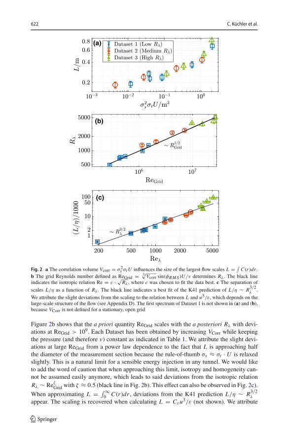
Fig. 2 a The correlation volume Vcorr = σ 2s σtU influences the size of the largest flow scales L = ∫

C(r)dr .b The grid Reynolds number defined as ReGrid = 3√Vcorr sin(φRMS)U/ν determines Rλ. The black lineindicates the isotropic relation Re = c · √

Rλ, where c was chosen to fit the data best. c The separation of

scales L/η as a function of Rλ. The black line indicates a best fit of the K41 prediction of L/η ∼ R3/2λ .

We attribute the slight deviations from the scaling to the relation between L and u3/ε, which depends on thelarge-scale structure of the flow (see Appendix D). The first spectrum of Dataset 1 is not shown in (a) and (b),because VCorr is not defined for a stationary, open grid

Figure 2b shows that the a priori quantity ReGrid scales with the a posteriori Rλ with devi-ations at ReGrid > 109. Each Dataset has been obtained by increasing VCorr while keepingthe pressure (and therefore ν) constant as indicated in Table 1. We attribute the slight devi-ations at large ReGrid from a power law dependence to the fact that L is approaching halfthe diameter of the measurement section because the rule-of-thumb σs ≈ σt · U is relaxedslightly. This is a natural limit for a sensible energy injection in any tunnel. We would liketo add the word of caution that when approaching this limit, isotropy and homogeneity can-not be assumed easily anymore, which leads to said deviations from the isotropic relationRλ ∼ Reζ

Grid with ζ ≈ 0.5 (black line in Fig. 2b). This effect can also be observed in Fig. 2c).

When approximating L = ∫ ∞0 C(r)dr , deviations from the K41 prediction L/η ∼ R3/2

λ

appear. The scaling is recovered when calculating L = Cεu3/ε (not shown). We attribute

123

Experimental Study of the Bottleneck in Fully Developed Turbulence 623

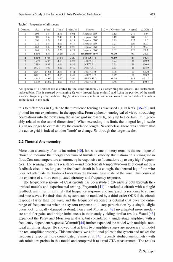
Table 1 Properties of all spectra

All spectra of a Dataset are distorted by the same function T ( f ) describing the sensor- and instrument-induced bias. This is ensured by changing Rλ only through large scales L and fixing the position of the smallscales in frequency space indicated by fη . A reference spectrum has been chosen from each dataset, which isemboldened in this table

this to differences in Cε due to the turbulence forcing as discussed e.g. in Refs. [36–39] andplotted for our experiments in the appendix. From a phenomenological of view, introducingcorrelations into the flow using the active grid increases Rλ only up to a certain limit (prob-ably related to the tunnel dimensions). When exceeding this limit, the integral length scaleL can no longer be estimated by the correlation length. Nevertheless, these data confirm thatthe active grid is indeed another ’knob’ to change Rλ through the largest scales.

2.2 Thermal Anemometry

More than a century after its invention [40], hot-wire anemometry remains the technique ofchoice to measure the energy spectrum of turbulent velocity fluctuations in a strong meanflow. Constant temperature anemometry is responsive to fluctuations up to very high frequen-cies. The sensing element’s resistance—and therefore its temperature—is kept constant by afeedback circuit. As long as the feedback circuit is fast enough, the thermal lag of the wiredoes not attenuate fluctuations faster than the thermal time scale of the wire. This comes atthe expense of a more complicated circuitry and frequency response.

The frequency response of CTA circuits has been studied extensively both through the-oretical models and experimental testing. Freymuth [41] linearized a circuit with a singlefeedback amplifier of infinitely flat frequency response and analyzed its response to squareand sine waves. He finds that the system can be modeled by a third-order ODE if the circuitresponds faster than the wire, and the frequency response is optimal (flat over the entirerange of frequencies) when the system response to a step perturbation by a single, slightovershoot (critically damped system). Perry and Morrison [42] investigated more moder-ate amplifier gains and bridge imbalances in their study yielding similar results. Wood [43]expanded the Perry and Morrison analysis, but considered a single-stage amplifier with afrequency-dependent response.Watmuff [44] further expanded themodel withmultiple, non-ideal amplifier stages. He showed that at least two amplifier stages are necessary to modelthe real amplifier properly. This introduces two additional poles to the system and makes thefrequency response more complicated. Samie et al. [45] recently studied anemometry withsub-miniature probes in this model and compared it to a real CTA measurement. The results

123

624 C. Küchler et al.

supported the further development of their in-house circuit, such that sub-miniature hot wireprobes could be operated successfully on this CTA for the first time.

These theoretical attempts to predict the frequency response of a CTA circuit are accompa-nied by experimental approaches. Bonnet and de Roquefort [46] heated the wire periodicallyby a perturbation voltage as well as laser heating to determing the frequency response. Weisset al. [47] used the aforementioned square wave test and interpreted its power spectrum asa measure for the frequency response curve. Hutchins et al. [48] exploited the well-definedfrequency content of pipe flow at different operating pressures to obtain frequency responsecurves without artificial heating. They were able to create flows of almost identical Reynoldsnumber, but different frequency content and could deduce the frequency-response curvesfor different circuits and wires. They compared several anemometer circuits and wires andfound that the frequency responses are non-constant at frequencies as low as 500 Hz. For thecombination of CTA circuit and wire used in the present study, they report an attenuationbetween 400 Hz and 7 kHz followed by a strong amplification of the signal. We thereforecannot assume a flat frequency response for ourmeasurements and adress these effects below.

The energy spectrum measured by a hot wire is influenced by the effects of finite wirelength. Length scales smaller than the sensor’s sensing lengths l will be attenuated, butalso larger wavenumbers are influenced. Wyngaard [49] used a Pao model spectrum [50] toinvestigate this attenuation of small scales. These resultswere reviewed inRef. [51] indicatingthat for l/η = 2, the attenuation of the one-dimensional spectrum is still minimal at kη ∼ 0.3,which was supported by Ashok et al. [52]. Sadeghi et al. [53] used sub-miniature hot wires(NSTAPs) as a benchmark and found that spatial filtering of the energy spectrum is minimalfor l/η < 3.7 at kη < 0.1.

In this study we used conventional hot wires of sensing length 450 µm for pressuresbelow 2 bar, as well as nanoscale thermal anemometry probes (NSTAP) of sensing length30 µm provided by Princeton University with a Dantec Dynamics StreamWare CTA circuit.The NSTAP is a 100 nm thick, 2.5 µm wide, and 30 or 60 µm long free-standing platinumfilm supported by a silicon structure and soldered to the prongs of a Dantec hot wire. Theproduction process and characteristics are detailed in Refs. [54–57]. For the conventional hotwire l/η < 5 in all cases and for the NSTAP l/η < 3. Therefore, η cannot be fully resolved inall cases. However, the bottleneck effect is typically found around 100η. The aforementionedreferences show that we can regard the distortions due to finite wire length as minor in thispart of the energy spectrum.

To summarize, the spatial resolution of our measurement instruments is sufficient to studythe Rλ-dependence of the bottleneck effect. Nevertheless the nonlinear frequency responseof the circuitry remains a source of systematic error that is different from random noiseoccuring at very high frequencies. Here we describe a procedure that takes the response intoaccount and thus removes this systematic measurement error.

3 Relative Spectra

3.1 The Concept

As outlined above, systematic errors influence the energy spectra recorded with a hot-wireanemometer. Formally, this means that the one-dimensional energy spectrum E11( f ) is dis-torted by a frequency-dependent transfer function T ( f ):

EM ( f ) = E11( f )T ( f )

123

Experimental Study of the Bottleneck in Fully Developed Turbulence 625

T ( f ) describes the effects of the thermal wire response, which depends on pressure andspeed, and the reponse of the constant temperature anemometry circuit. Ideally, T ( f ) isa constant over the whole range of relevant frequencies, but the evidence detailed aboveindicates a complex shape of amplification and attenuation of the signal. In this study we donot make any attempt to find T ( f ). Instead, we control its effects by keeping T ( f ) the samefor several flows at different Rλ.

To ensure that the spectra only differ because of changes in the turbulent fluctuation andnot because of the frequency response curve of the anemometer, we need to ensure that theresponse curve T ( f ) is unaltered between spectra. We achieve this in two steps. The ambientpressure might influence the heat transfer of the wire and therefore T ( f ). Furthermore, T ( f )is influenced by the CTA tuning (in particular the overheat), and the sensor itself. Therefore,we fix the ambient pressure within a set of spectra (a ’Dataset’) and measure using the samesensor and the same CTA settings.

The second step is to ensure that a given kη is influenced by the same part of the frequencyresponse curve T ( f ). Thus, we need to fix the position of a spectral feature in frequencyspace. This means that the mean velocity U must be the same within one Dataset. T ( f )mainly distorts the small-scale end of the spectrum [41–45,47,48,51], whose location infrequency space at a given U is determined by the kinematic viscosity ν. ν is fixed within aDataset because the pressure remains constant.

We can, however, change the energy injection scale and thus Rλ with the autonomousactive grid. This way we can conduct measurements at different Rλ. Ultimately, we caneliminate T ( f ) by relating each spectrum to a reference spectrum:

EiM ( f )

ERefM ( f )

= Ei11( f )T

i ( f )

ERef11 ( f )TRef( f )

= Ei11( f )T ( f )

ERef11 ( f )T ( f )

= Ei11(kU/2π)

ERef11 (kU/2π)

. (2)

In the following we call the ratio of a spectra divided by a reference spectrum in the frequncydomain, relative spectrum. We emphasize that the notion of relative spectra is not necessaryto investigate Rλ-scaling within one Dataset prepared in the aforementioned way. However,the accessible range of Rλ by changing only the active grid forcing is limited. Therefore,several of such Datasets with different frequency distortions need to be prepared by changingkinematic viscosity ν andmean flow speedU to obtain a convincing scaling range. The notionof relative spectra is then required to compare those Datasets.

3.2 Results

We created three sets of spectra that have identical T ( f ) each. We call these sets ‘Datasets‘.Table 1 shows important parameters for each spectrum. Note that L changes significantlywithin a given dataset leading to changes in Rλ, while fη = U/η remains almost constantwithin the dataset. This indicates that we changed Rλ only by increasing the large scales,while keeping all small-scale features of the spectrum at the same frequency. For example, inDataset 2, the peak of the spectral bump always lies at a frequency of ∼ 700 Hz, whereas thebeginning of the inertial range spans a factor of 4 in frequency (2 to 8 Hz). This exemplifiesthe excellent control over Rλ permitted by the autonomous active grid as indicated in Fig. 2.

The lower graphs of Figs. 3, 4 and 5 show the spectra from each of the respective datasetsdivided by the reference spectrum ERef

11 . ERefM is plotted pre-compensated in the upper graphs

123

626 C. Küchler et al.

Fig. 3 Reference spectrum at Rλ = 1305 (upper plot) and relative spectra from Dataset 1. The data have beencollapsed at kη = 0.015, which we defined as the beginning of the bottleneck region.We identified the peaks inthe relative spectra with the bottleneck peak of the absolute spectra. The peak height decreased with increasingRλ and different spectra of similar Rλ result in very similar relative spectra as expected. Furthermore, theslope of the spectrum at kη < 0.015 seems to decrease with Rλ. The shaded areas are a measure of the noiselevel

Fig. 4 Reference spectrum at Rλ = 1308 (upper plot) and relative spectra from Dataset 2. The trends in peakheight and slope from Fig. 3 continue

123

Experimental Study of the Bottleneck in Fully Developed Turbulence 627

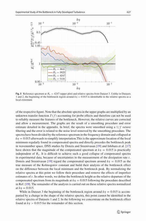
Fig. 5 Reference spectrum at Rλ = 4247 (upper plot) and relative spectra from Dataset 3. Unlike in Datasets1 and 2, the beginning of the bottleneck region around kη = 0.015 is identifiable in the relative spectra as alocal extremum

of the respective figure. Note that the absolute spectra in the upper graphs aremultiplied by anunknown transfer function T ( f ) accounting for probe effects and therefore can not be usedto reliably measure the features of the bottleneck. However, the relative curves are correctedand allow a measurement. The graphs are the result of a smoothing procedure and errorestimate detailed in the appendix. In brief, the spectra were smoothed using a 1/ f octavefiltering and the error is related to the noise level removed by the smoothing procedure. Thespectra have been divided by the reference spectrum in the frequency domain and collapsed atkη = 0.015 afterwards to simplify interpretation.This is the approximate location of the localminimum regularly found in compensated spectra and directly precedes the bottleneck peakin wavenumber space. DNS studies by Donzis and Sreenivasan [19] and Ishihara et al. [17]have shown that the magnitude of the compensated spectrum at kη = 0.015 is practicallyindependent of Rλ. It is difficult to achieve such a good collapse of compensated spectrain experimental data, because of uncertainties in the measurement of the dissipation rate ε.Donzis and Sreenivasan [19] regard the compensated spectrum around kη = 0.015 as thetrue measure of the Kolmogorov constant and build their analysis of the bottleneck effecton the difference between the local minimum and the bottleneck peak. By normalizing therelative spectra at this point we follow their procedure and remove the effects of imperfectestimates of ε. In other words, we define the bottleneck height as the relative departure of thecompensated spectrum from its magnitude at kη = 0.015 following the procedure describedin Ref. [19]. The remainder of the analysis is carried out on these relative spectra normalizedat kη = 0.015.

While in Dataset 3 the beginning of the bottleneck region around kη = 0.015 is accom-panied by a change in the shape of the relative spectra, this point cannot be identified in therelative spectra of Datasets 1 and 2. In the following we concentrate on the bottleneck effectfound at kη > 0.015 for the remainder of this section.

123

628 C. Küchler et al.

The location of the spectral bump forming the bottleneck effect in relative spectra isnot obvious. Our data from one-dimensional spectra suggests that the peak occurs betweenkη = 0.03 and kη = 0.06, which is consistent with the findings from DNS, where thepeak typically occurs at kη = 0.046 in the one-dimensional spectra (see e.g. Refs. [19],[17]). However, when considering the background noise, the peak location is not the majorsource of error. E.g. for Rλ = 1539, all points between 0.015 < kη < 0.07 are within theerrorband at kη = 0.05. We therefore define the extremum in the relative spectrum between0.015 < kη < 0.08 as the relative height h of the bottleneck effect. This has the additionaladvantage to be independent of the errors in the estimate of η. To preclude biases from thisdefinition, we repeat our analysis with different definitions of the relative bottleneck heightin Fig. 11 in the appendix.

Finally, the measured bottleneck height cannot depend on which spectrum is chosen asreference. We have calculated the bottleneck height with all possible choices of ERef

11 andfound our results to be largely independent of that choice (see Appendix for details).

Figure 6 shows the bottleneck height—defined as above—as a function of Rλ/RRefλ within

each dataset. The data shows a trend towards smaller peak heights in the relative spectrumwithincreasing Rλ. The data follows the numerical data we have compiled from various sources[17,58–60].Wehave analyzed the data fromBuaria et al. [60] at Rλ up to 1000 (Rλ/RRef

λ < 1).The increased small-scale resolution in comparison to [19] seems to have no noticable impacton the bottleneck. Therefore, this data at is practically the same as the one used by Donzis &Sreenivasan [19] for our purposes. The data from Rλ = 1300 (Rλ/RRef

λ = 1) was reportedin Ref. [58]. The numerical data at Rλ/RRef

λ ≈ 1.9, which corresponds to Rλ = 2340, is thehighest Rλ reported by Ishihara et al. [17]. The relative spectra of the numerical data wereanalyzed equivalently to the experimental data and the spectrum at Rλ = 1300 was chosenas a reference spectrum. We have used the one-dimensional spectra in our analysis of thenumerical data.

When excluding the lowest Rλ, the experimental data is in agreement with the power lawof

h ∼ (Rλ/R

Refλ

)−0.061±0.007.

The fit was obtained by a bootstrap procedure based on the error bars. It compares well withthe findings of Donzis and Sreenivasan [19], who report a bottleneck scaling of h ∼ R−0.04

λ .Their analysis similarly defines the bottleneck height as the difference between the heightof the compensated spectrum at the bottleneck peak and the local minimum preceding thispeak.

The spectrum at Rλ = 193 follows the general trend of decreasing peak height with Rλ,but its peak differs substantially from the predictions. The absolute spectrum (not shown)exhibits no signs of a 5/3-scaling, and consequently the bottleneck region cannot be clearlyseparated from the rest of the spectrum. This is substantially different from the other spectra,where the end of the integral range could always be observed in the absolute spectra and wetherefore are not surprised that the relative spectrum at Rλ = 193 deviates from the remainderof the data. This spectrum has consequently been ignored in our interpretation.

Further, we can change Rλ only by a factor of 5 through the autonomous active grid.WhileDataset 1 and 2 each feature a spectrum at the same Rλ, there is a gap between the highest Rλ

of Dataset 2 (2704) and the lowest of Dataset 3 (3641). To plot h as a function of Rλ alone,we use the aforementioned power law fit from Fig. 6. Under this assumption we can bridgethe gap between the two datasets, because h1/h2 = (Rλ1/Rλ2)

−0.0061±0.007. Using the finalpoint of Dataset 2 as Rλ1 = 2704 and the corresponding height h1 we can construct h2 usingthe lowest Rλ2 = 3641 from Dataset 3 to arrive at Fig. 7

123

Experimental Study of the Bottleneck in Fully Developed Turbulence 629

0.2 0.5 1 2

1

1.1

1.2

1.3

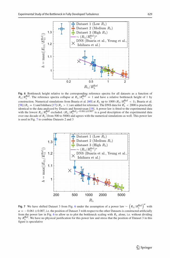
Fig. 6 Bottleneck height relative to the corresponding reference spectra for all datasets as a function ofRλ/RRef

λ . The reference spectra collapse at Rλ/RRefλ = 1 and have a relative bottleneck height of 1 by

construction. Numerical simulations from Buaria et al. [60] at Rλ up to 1000 (Rλ/RRefλ < 1), Buaria et al.

[58] (Rλ = 1) and Ishihara [17] (Rλ > 1 ) are added for reference. The DNS data for Rλ < 2000 is practicallyidentical to the data analyzed by Donzis and Sreenivasan [19]. A power law is fitted to the experimental datawith the lowest Rλ/RRef

λ excluded. (Rλ/RRefλ )−0.061±0.007 is a good description of the experimental data

over one decade of Rλ (from 500 to 5000) and agrees with the numerical simulations as well. This power lawis used in Fig. 7 to combine Datasets 2 and 3

200 500 1000 2000 5000

1

1.1

1.2

1.3

Fig. 7 We have shifted Dataset 3 from Fig. 6 under the assumption of a power law ∼(Rλ/RRef

λ

)αwith

α = − 0.061±0.007, i.e. the position of Dataset 3 with respect to the other Datasets is constructed artificiallyfrom the power law in Fig. 6 to allow us to plot the bottleneck scaling with Rλ alone, i.e. without dividingby RRef

λ . We have no physical justification for this power law and stress that the position of Dataset 3 in thisfigure is speculative

123

630 C. Küchler et al.

4 Discussion

In this paper we studied the spectra of a turbulent wind tunnel flow of Rλ between 193and 5131. We have used regular hot-wires as well as NSTAPs with a state-of-the-artconstant temperature anemometer to record single-point two-time statistics of the tur-bulent fluctuations, in particular energy spectra. However, such spectra can be heavilyinfluenced by non-ideal frequency responses of the circuit. The frequency response is par-ticularly complicated when operating sub-miniature wires like the NSTAP with a CTA[45,48]. A constant current anemometer (CCA) might perform better in this respect, becausethe frequency reponse is limited only by the thermal lag of the wire and no feedbackloop is involved. Still, this comes at the expense of a variable wire temperature and -resistance.

In an attempt to interpret CTA data suffering from a non-flat frequency response, we con-sider energy spectra relative to a reference spectrum. Such an analysis significantly restrictsthe phenomena that can be observed. The bump in the energy spectrum at the transition fromthe inertial to the dissipation range can still be identified in the relative spectra as a localextremum beyond kη = 0.015.

To the best of our knowledge, no other wind tunnel achieves Rλ > 5000 in a gas. More-over, we do not know of any other quantitative study of the scaling of the bottleneck effectwith Rλ in a laboratory experiment. We attribute this to the difficulties one faces when inter-preting energy spectra from CTAmeasurements at relatively high frequencies: The spectrumis stronlgy influenced by the CTA circuitry and these influences are hard to quantify oreliminate.

With the aforementioned procedures we are able to extract information about the bottle-neck effect from instrument-distorted hot wire spectra.We find indications that the bottleneckeffect decreases up to Rλ ∼ 5000.Wefit a power lawof (Rλ/RRef

λ )−α withα = 0.061±0.007,which is close to the value of (Rλ)

−0.04 found by Donzis and Sreenivasan [19]. Theirnumerical results are in general in good agreement with our experimental data, lendingsupport to the experiment and data anlysis procedure. Our data equally supports Vermaand Donzis [11], who predict that the bottleneck scales as h ∼ 1 − γ (1.5 log2(Rλ))

2/3.Revisiting Fig. 6, the data is not inconsistent with different Rλ/RRef

λ -scalings of the rela-tive bottleneck height in the different datasets. We have therefore calculated the scaling ofthe individual datasets and found that while Dataset 2 and 3 have almost identical scalingexponents (− 0.032 ± 0.012, and − 0.034 ± 0.029, respectively), Dataset 1 shows a scalingof − 0.1528 ± 0.012. When excluding the two lowest Rλ, the scaling exponent becomes− 0.083 ± 0.024. This points towards different behaviours at low Rλ, probably due to theeffects of a not properly developed inertial range, which contaminates the bottleneck scal-ing. Such a claim is supported by the slopes of the spectra at 0.001 < kη < 0.015, whichclearly get steeper with increasing Rλ in Dataset 1, but change very little in Datasets 2and 3, indicating a properly developed inertial range. Interestingly, this effect cannot beseen in DNS, where the bottleneck scaling of R−0.04

λ can be found at low Reynolds num-bers.

We attempt to plot the relative bottleneck height as a function of Rλ alone. This requiresthe assumption that the aforementioned power law holds and can be extrapolated. Such anassumption is highly speculative and the results should be considered as such.

We can not quantify the absolute height of the bottleneck bump. Yet, we can argue thatif the relative spectra are still changing with Rλ in the relevant region, the effect has notcompletely vanished. We can find a systematic decrease of the peak in the relative spectra

123

Experimental Study of the Bottleneck in Fully Developed Turbulence 631

for Rλ < 3000. The data for Rλ > 3000 in Dataset 3 is inconclusive. A small, decreasingtrend can be found, consistent with the power law fit. However, the differences in heightare so small compared to the error bars that the claim of a constant bottleneck height atRλ > 3000 would also be supported by the data, especially when considering alternativedefinitions of the bottleneck height in relative spectra as in Fig. 11 found in the appendix.This is not in contradiction to the atmospheric spectra mentioned above, as they have aneven higher Rλ. Further, we note that a bottleneck effect might not show up as a peak in a5/3-compensated spectrum, yet might be present when compensating by an intermittency-corrected slope −(5/3 + β). In this case, the bottleneck effect would still be visible in therelative spectrum. However, the claim that the bottleneck height does not change with Rλ forRλ > 3000 is not ruled out by the data.

As far as this study is concerned, the data matches the predictions of Verma and Donzis[11]: The bottleneck height decreases with increasing Rλ, but relatively high Rλ are neces-sary to make the effect vanish completely. Based on nonlinear and nonlocal shell-to-shellenergy transfer Verma and Donzis [11] estimate that the bottleneck is basically absent forRλ > 104, but acknowledge that this might be an overestimate. While lending supportto existing studies of the bottleneck effect, especially [19] and theories that incorporate aRλ-dependence of the peak height, an investigation of the effect in terms of absolutemeasure-ments of spectra seems necessary to confirm these claims experimentally. With subminiatureprobes of low thermal lag, such a study might be possible with a constant current anemome-ter, whose frequency response is intriniscally more simple. However, the present study couldreliably measure how the bottleneck decreases with increasing Rλ for the first time in anlaboratory experiment and for Rλ much higher than achieved in DNS or other wind tunnelstudies.

Acknowledgements Open access funding provided by Max Planck Society. The operation of the experimentwould be impossible without the help and expertise of A. Kubitzek, A. Kopp, A. Renner, U. Schminke and O.Kurre. The NSTAPs were generously provided by M. Hultmark and Y. Fan. We thank P. K. Yeung, D. Buaria,and T. Ishihara for providing the numerical data. We thank D. Lohse and P. Roche for useful comments.

OpenAccess This article is distributed under the terms of the Creative Commons Attribution 4.0 InternationalLicense (http://creativecommons.org/licenses/by/4.0/),which permits unrestricted use, distribution, and repro-duction in any medium, provided you give appropriate credit to the original author(s) and the source, providea link to the Creative Commons license, and indicate if changes were made.

Appendix A: Brief Description of theWind Tunnel

The VDTT consists of two 11.7 m long straight cylindrical tubes connected by two elbows ofcenter-line radius of 1.75 m. The tunnel was filled with sulfur-hexaflouride (SF6) at pressuresbetween 1.5 and 15 bar for the measurements presented here.

The flow is propelled by a fan rotating at up to 24 Hz creating mean flow speeds ofup to 5.5 m/s. It passes the first elbow and enters a heat exchanger, which removes anyturbulent energy dissipated into heat and thus keeps the temperature in the tunnel constant.The rectangular cross-section of the heat exchanger is smoothly adapted to the tunnel’scircular geometry by contractions. The vertical slots of the heat exchanger are expected todestroy large-scales structure present in the flow. After the heat exchanger, the flow passesan 80 cm long expansion, which adapts it to the measurement section. While passing thisexpansion the flow is stabilized and homogenized by three consecutive meshes of ascendingspacing. The flow enters a 9 m long measurement section through an 104 cm high active grid,

123

632 C. Küchler et al.

which is directly followed by a 70 cm long expansion to the measurement section’s heightof 117 cm. The measurement section is followed by another elbow and enters a secondmeasurement section through another sequence of three meshes before being acceleratedagain by the fan.

Appendix B: Data Acquisition and Analysis Procedure

TheNSTAPswere operated following largely [61] using aDantec StreamLine 90C10modulewithin a 90N10 frame. The CTA bridge was set to a 1:1 ratio and the overheat is determinedby an external resistor Rext connected to the system. Typical overheat ratios Rext/RProbe

were 1.2–1.3, where RProbe ∼ 100� denotes the probe cold resistance. The Dantec wireswere used in a 1:20 bridge utilizing the internal automatics to set the overheat. The data wasacquired in the following procedure: The hot wire frequency response and proper operationwas tested on a very basic level using the square wave test built into the Dantec CTA-system.The hot-wire system was calibrated by scanning a range of mean flow speeds set by the fanfrequency in the tunnel. We determined the mean flow speed through the differential pressurebetween a pitot tube and a static pressure probe. The differential pressure was picked up bya Siemens SITRANS differential pressure transfucer/ We chose ∼ 20 calibration pointsspaced by ∼ 0.1 m/s. The probe voltage was recorded for 60 s along with the mean pressuredifference, a voltage-velocity curve was calculated, and King’s law was fitted to the data. Inbetween calibration points we waited for 45 s for the mean flow to become stationary. Thedata was recorded with a National Instruments NI PCI-6123 16-bit DAQ-Card at samplingrates of 60 or 200 kHz. Higher sampling rates were used for NSTAP measurements, wherethe CTA analog low-pass filter was set to 100 kHz. When using standard hot wires, thefilter frequency was set to 30 kHz and the data was sampled at 60 kHz. The data wasrecorded in segments of 6 million voltage samples, each saved to disk in a 16-bit binaryformat.

We shall briefly outline the initial data analysis procedure used to obtain essential tur-bulence statistics as well as the power spectrum. Each of the following steps was carriedout on each segment and the results were averaged over all files in the end. We used King’slaw with parameters obtained from the calibration data to convert the voltages to veloci-ties. Note that the shape of the energy-frequency spectrum is independent of the calibration,which is only required to obtain its absolute value. Because the analog filtering was notsufficient to filter out all noise, we low-pass filtered the data digitally using a butterworth-Filter of order 3 in forward and reverse directions. This introduces edge effects, whichwe remove by cutting the first and last 60 points of the time series. We then subtract themean U from the velocity time series to obtain a time series of u. The remaining analysisis performed on this filtered dataset. The power spectra were calculated using MATLB’sfft function, which is based on the FFTW-package . We calculate the correlation functionusingMATLAB’s xcorr function, which itself relies on the aforementioned fourier transformprocedure as well as structure functions of order 1 to 8. Finally, we obtain histograms ofvelocity and voltage. We use Taylor’s Hypothesis, which assumes that a one-dimensionalvelocity field can be obtained from a time series by multiplying the time increments by themean velocity: �x = �t · U . The power spectra are normalized using the assumption that∫E(k)dk = u2.We routinely calculate basic turbulence quantities in different ways and check the results

for consistency. The quantites Rλ, and η depend on the mean energy dissipation rate ε,

123

Experimental Study of the Bottleneck in Fully Developed Turbulence 633

which we measure using the third-order structure function S3(r) = 〈(u(x + r) − u(x))3〉 =4/5(εr). The last step follows from the Navier-Stokes equations and is also predicted byKolmogorov’s 1941 theory. In practice we estimate ε = max(5/4 S3/r) and check the resultwith ε = 15ν

∫k2E(k)dk, and ε = max(S3/22 /r). The integral length scale is calculated as

L = ∫ ∞0 C(r)dr , where C(r) = 〈u(x + r)u(x)〉 is the velocity auto-correlation function. Its

error mainly stems from the ambiguous choice of the upper integration limit, which leads toa relative error about 10% in L .

Appendix C: Calculation and Cross-Check of Relative Spectra

To obtain relative spectra, the initial spectrum consisting of 3 million points was downsam-pled to 50 000 logarithmically spaced datapoints. To remove the noise from these spectra,we have smoothed them using a fractional octave smoothing algorithm. It multiplies thespectrum at each frequency with a Gaussian centered around the current frequency fi with awidth of σi = ( fi/n)/π , where n determines the smoothing level. Therefore, the smoothingwindow is larger for higher frequencies. To estimate the noise level in the spectrum and theassociated statistical error, we consider the data within 3σi of each frequency.We estimate thestandard error as δ = √

Var/N , where N is the number of points considered and Var denotestheir variance. Finally, the compensated spectra are calculated as ψ(k) = E11(k)k5/3ε−2/3,which can be written as ψ( f ) by Taylor’s Hypothesis. Finally, we divide the i-th spec-trum in a dataset by the reference spectrum: ψi ( f )/ψRef( f ). The result is normalized atkη = 0.015 to remove offsets introduced by uncertainties in ε and to simplify compar-isons.

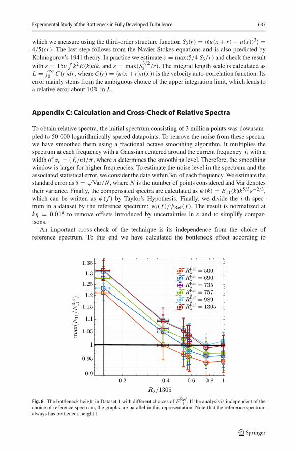
An important cross-check of the technique is its independence from the choice ofreference spectrum. To this end we have calculated the bottleneck effect according to

Fig. 8 The bottleneck height in Dataset 1 with different choices of ERef11 . If the analysis is independent of the

choice of reference spectrum, the graphs are parallel in this representation. Note that the reference spectrumalways has bottleneck height 1

123

634 C. Küchler et al.

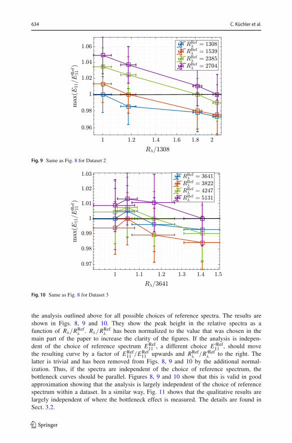
Fig. 9 Same as Fig. 8 for Dataset 2

Fig. 10 Same as Fig. 8 for Dataset 3

the analysis outlined above for all possible choices of reference spectra. The results areshown in Figs. 8, 9 and 10. They show the peak height in the relative spectra as afunction of Rλ/RRef

λ . Rλ/RRefλ has been normalized to the value that was chosen in the

main part of the paper to increase the clarity of the figures. If the analysis is indepen-dent of the choice of reference spectrum ERef

11 , a different choice E ′Ref11 , should move

the resulting curve by a factor of ERef11 /ERef

11 upwards and RRefλ /R′Ref

λ to the right. Thelatter is trivial and has been removed from Figs. 8, 9 and 10 by the additional normal-ization. Thus, if the spectra are independent of the choice of reference spectrum, thebottleneck curves should be parallel. Figures 8, 9 and 10 show that this is valid in goodapproximation showing that the analysis is largely independent of the choice of referencespectrum within a dataset. In a similar way, Fig. 11 shows that the qualitative results arelargely independent of where the bottleneck effect is measured. The details are found inSect. 3.2.

123

Experimental Study of the Bottleneck in Fully Developed Turbulence 635

0.5 1 1.5 2

1

1.05

1.1

0.5 1 1.5 2

1

1.05

1.1

0.5 1 1.5 2

1

1.05

1.1

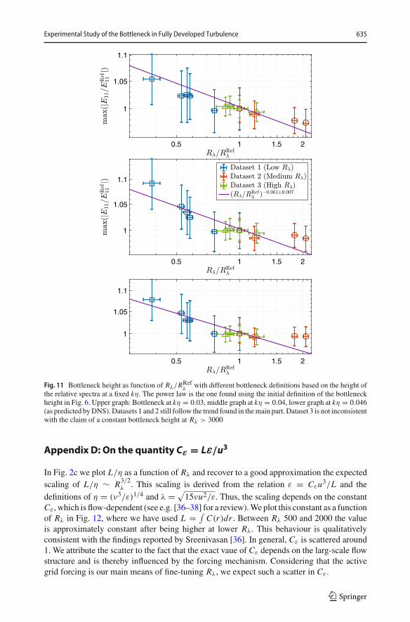
Fig. 11 Bottleneck height as function of Rλ/RRefλ with different bottleneck definitions based on the height of

the relative spectra at a fixed kη. The power law is the one found using the initial definition of the bottleneckheight in Fig. 6. Upper graph: Bottleneck at kη = 0.03, middle graph at kη = 0.04, lower graph at kη = 0.046(as predicted byDNS).Datasets 1 and 2 still follow the trend found in themain part. Dataset 3 is not inconsistentwith the claim of a constant bottleneck height at Rλ > 3000

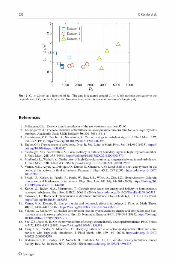
Appendix D: On the quantity C" = L"/u3

In Fig. 2c we plot L/η as a function of Rλ and recover to a good approximation the expectedscaling of L/η ∼ R3/2

λ . This scaling is derived from the relation ε = Cεu3/L and the

definitions of η = (ν3/ε)1/4 and λ = √15νu2/ε. Thus, the scaling depends on the constant

Cε, which is flow-dependent (see e.g. [36–38] for a review).We plot this constant as a functionof Rλ in Fig. 12, where we have used L = ∫

C(r)dr . Between Rλ 500 and 2000 the valueis approximately constant after being higher at lower Rλ. This behaviour is qualitativelyconsistent with the findings reported by Sreenivasan [36]. In general, Cε is scattered around1. We attribute the scatter to the fact that the exact vaue of Cε depends on the larg-scale flowstructure and is thereby influenced by the forcing mechanism. Considering that the activegrid forcing is our main means of fine-tuning Rλ, we expect such a scatter in Cε.

123

636 C. Küchler et al.

0 1000 2000 3000 4000 5000 60000

0.5

1

1.5

2

2.5

3

Fig. 12 Cε = Lε/u3 as a function of Rλ. The data is scattered around Cε = 1. We attribute the scatter to thedependence of Cε on the large scale flow structure, which is our main means of changing Rλ

References

1. Fefferman, C.L.: Existence and smoothness of the navier-stokes equation 57, 672. Kolmogorov, A.: The local structure of turbulence in incompressible viscous fluid for very large reynolds

numbers. Akademiia Nauk SSSR Doklady 30, 301–305 (1941)3. Sreenivasan, K.R., Prabhu, A., Narasimha, R.: Zero-crossings in turbulent signals. J. Fluid Mech. 137,

251–272 (1983). https://doi.org/10.1017/S00221120830023964. Taylor, G.I.: The spectrum of turbulence. Proc. R. Soc. Lond. AMath. Phys. Sci. 164, 919 (1938). https://

doi.org/10.1098/rspa.1938.00325. Saddoughi, S.G., Veeravalli, S.V.: Local isotropy in turbulent boundary layers at high Reynolds number.

J. Fluid Mech. 268, 333 (1994). https://doi.org/10.1017/S00221120940013706. Mydlarski, L.,Warhaft, Z.: On the onset of high-Reynolds-number grid-generatedwind tunnel turbulence.

J. Fluid Mech. 320, 320–331 (1996). https://doi.org/10.1017/S00221120960075627. Verma, M.K., Ayyer, A., Debliquy, O., Kumar, S., Chandra, A.V.: Local shell-to-shell energy transfer via

nonlocal interactions in fluid turbulence. Pramana J. Phys. 65(2), 297 (2005). https://doi.org/10.1007/BF02898618

8. Frisch, U., Kurien, S., Pandit, R., Pauls, W., Ray, S.S., Wirth, A., Zhu, J.Z.: Hyperviscosity, Galerkintruncation, and bottlenecks in turbulence. Phys. Rev. Lett. 101(14), 144501 (2008). https://doi.org/10.1103/PhysRevLett.101.144501

9. Kurien, S., Taylor, M.A., Matsumoto, T.: Cascade time scales for energy and helicity in homogeneousisotropic turbulence. Phys. Rev. E 69(6), 066313 (2004). https://doi.org/10.1103/PhysRevE.69.066313

10. Falkovich, G.: Bottleneck phenomenon in developed turbulence. Phys. Fluids 6(4), 1411–1414 (1994).https://doi.org/10.1063/1.868255

11. Verma, M.K., Donzis, D.: Energy transfer and bottleneck effect in turbulence. J. Phys. A: Math. Theor.40(16), 4401–4412 (2007). https://doi.org/10.1088/1751-8113/40/16/010

12. Yakhot, V., Zakharov, V.: Hidden conservation laws in hydrodynamics; energy and dissipation rate fluc-tuation spectra in strong turbulence. Phys. D: Nonlinear Phenom. 64(4), 379–394 (1993). https://doi.org/10.1016/0167-2789(93)90050-B

13. She, Z.S., Jackson, E.: On the universal form of energy spectra in fully developed turbulence. Phys. FluidsA 5(7), 1526–1528 (1993). https://doi.org/10.1063/1.858591

14. Kang, H.S., Chester, S., Meneveau, C.: Decaying turbulence in an active-grid-generated flow and com-parisons with large-eddy simulation. J. Fluid Mech. 480, 129–160 (2003). https://doi.org/10.1017/S0022112002003579

15. Bodenschatz, E., Bewley, G.P., Nobach, H., Sinhuber, M., Xu, H.: Variable density turbulence tunnelfacility. Rev. Sci. Instrum. 85(9), 093908 (2014). https://doi.org/10.1063/1.4896138

123

Experimental Study of the Bottleneck in Fully Developed Turbulence 637

16. Khurshid, S., Donzis, D.A., Sreenivasan, K.R.: Energy spectrum in the dissipation range. Phys. Rev.Fluids 3, 8 (2018). https://doi.org/10.1103/PhysRevFluids.3.082601

17. Ishihara, T., Morishita, K., Yokokawa, M., Uno, A., Kaneda, Y.: Energy spectrum in high-resolutiondirect numerical simulations of turbulence. Phys. Rev. Fluids 1, 8 (2016). https://doi.org/10.1103/PhysRevFluids.1.082403

18. Ishihara, T., Kaneda, Y., Yokokawa, M., Itakura, K., Uno, A.: Energy spectrum in the near dissipationrange of high resolution direct numerical simulation of turbulence. J. Phys. Soc. Jpn. 74(5), 1464–1471(2005). https://doi.org/10.1143/JPSJ.74.1464

19. Donzis, D.A., Sreenivasan, K.R.: The best bottleneck effect and the Kolmogorov constant in isotropicturbulence. J. Fluid Mech. 657, 171–188 (2010). https://doi.org/10.1017/S0022112010001400

20. Gulitski, G., Kholmyansky, M., Kinzelbach, W., Lüthi, B., Tsinober, A., Yorish, S.: Velocity and tem-perature derivatives in high-Reynolds-number turbulent flows in the atmospheric surface layer. Part 1.Facilities, methods and some general results. J. Fluid Mech. 589, 57–81 (2007). https://doi.org/10.1017/S0022112007007495

21. Sreenivasan, K.R., Dhruva, B.: Is there scaling in high-Reynolds-number turbulence? Prog. Theor. Phys.Suppl. 130, 103–120 (1998). https://doi.org/10.1143/PTPS.130.103

22. Tsuji, Y.: Intermittency effect on energy spectrum in high-reynolds number turbulence. Phys. Fluids 16,L43–L46 (2004). https://doi.org/10.1063/1.1689931

23. Dobler, W., Haugen, N.E.L., Yousef, T.A., Brandenburg, A.: Bottleneck effect in three-dimensional tur-bulence simulations. Phys. Rev. E 68(2), 026304 (2003). https://doi.org/10.1103/PhysRevE.68.026304

24. Lohse, D.,Mueller-Groeling, A.: Bottleneck effects in turbulence: scaling phenomena in r-versus p-space.Phys. Rev. Lett. 74(10), 1747–1750 (1995). https://doi.org/10.1103/PhysRevLett.74.1747

25. Sinhuber, M., Bewley, G.P., Bodenschatz, E.: Dissipative effects on inertial-range statistics at highReynolds numbers. Phys. Rev. Lett. 119(13), 134502 (2017). https://doi.org/10.1103/PhysRevLett.119.134502

26. Taylor, G.I.: Statistical theory of turbulence. Proc. R. Soc. Lond. AMath. Phys. Sci. 151(873), 421 (1935).https://doi.org/10.1098/rspa.1935.0158

27. Yeung, P.K., Sreenivasan, K.R., Pope, S.B.: Effects of finite spatial and temporal resolution in directnumerical simulations of incompressible isotropic turbulence. Phys. Rev. Fluids 3(6), 064603 (2018).https://doi.org/10.1103/PhysRevFluids.3.064603

28. Bourgoin, M., Baudet, C., Kharche, S., Mordant, N., Vandenberghe, T., Sumbekova, S., Stelzenmuller,N., Aliseda, A., Gibert, M., Roche, P.E., Volk, R., Barois, T., Caballero, M.L., Chevillard, L., Pinton, J.F.,Fiabane, L., Delville, J., Fourment, C., Bouha, A., Danaila, L., Bodenschatz, E., Bewley, G., Sinhuber,M., Segalini, A., Örlü, R., Torrano, I., Mantik, J., Guariglia, D., Uruba, V., Skala, V., Puczylowski, J.,Peinke, J.: Investigation of the small-scale statistics of turbulence in the Modane S1MAwind tunnel 9(2),269–281. https://doi.org/10.1007/s13272-017-0254-3

29. Pietropinto, S., Poulain, C., Baudet, C., Castaing, B., Chabaud, B., Gagne, Y., Hebral, B., Ladam, Y.,Lebrun, P., Pirotte, O., Roche, P.: Superconducting instrumentation for high Reynolds turbulence exper-iments with low temperature gaseous helium. Phys. C 386, 512–516 (2003)

30. Salort, J., Chabaud, B., Leveque, E., Roche, P.E.: Energy cascade and the four-fifths law in superfluidturbulence. Europhys. Lett. 97(3), 34006 (2012). https://doi.org/10.1209/0295-5075/97/34006

31. Rousset, B., Bonnay, P., Diribarne, P., Girard, A., Poncet, J.M., Herbert, E., Salort, J., Baudet, C., Castaing,B., Chevillard, L., Daviaud, F., Dubrulle, B., Gagne, Y., Gibert, M., Hebral, B., Lehner, T., Roche, P.E.,Saint-Michel, B., BonMardion,M.: Superfluid high Reynolds vonKármán experiment. Rev. Sci. Instrum.85(10), 103908 (2014). https://doi.org/10.1063/1.4897542

32. Saint-Michel, B., Herbert, E., Salort, J., Baudet, C., BonMardion,M., Bonnay, P., Bourgoin,M., Castaing,B., Chevillard, L., Daviaud, F., Diribarne, P., Dubrulle, B., Gagne, Y., Gibert, M., Girard, A., Hébral, B.,Lehner, T., Rousset, B.: SHREK collaboration: probing quantum and classical turbulence analogy in vonKármán liquid helium, nitrogen, and water experiments. Phys. Fluids 26(12), 125109 (2014). https://doi.org/10.1063/1.4904378

33. Sinhuber, M., Bodenschatz, E., Bewley, G.P.: Decay of turbulence at high Reynolds numbers. Phys. Rev.Lett. 114, 3 (2015). https://doi.org/10.1103/PhysRevLett.114.034501

34. Hideharu, M.: Realization of a large-scale turbulence field in a small wind tunnel. Fluid Dyn. Res. 8(1),53–64 (1991). https://doi.org/10.1016/0169-5983(91)90030-M

35. Griffin, K.P., Wei, N.J., Bodenschatz, E., Bewley, G.P.: Control of long-range correlations in turbulence.Exp. Fluids (2019). arXiv preprint arXiv:1809.05126

36. Sreenivasan, K.: On the scaling of the turbulence energy dissipation rate. Phys. Fluids 27(5), 1048–1051(1984). https://doi.org/10.1063/1.864731

37. Sreenivasan, K.: An update on the scaling of the turbulence energy dissipation rate. Phys. Fluids 10, 2(1998). https://doi.org/10.1063/1.869575

123

638 C. Küchler et al.

38. Vassilicos, C.: Dissipation in turbulent flows annular review of fluid mechanics 47, 1 (2015). https://doi.org/10.1146/annurev-fluid-010814-014637

39. Bewley, G., Chang, K., Bodenschatz, E.: On integral length scales in anisotropic turbulence. Phys. Fluids24, 6 (2012). https://doi.org/10.1063/1.4726077

40. Comte-Bellot, G.: Hot-wire anemometry 8(1), 209–231. https://doi.org/10.1146/annurev.fl.08.010176.001233

41. Freymuth, P.: Frequency response and electronic testing for constant-temperature hot-wire anemometers.J. Phys. E: Sci. Instrum. 10(7), 705 (1977). https://doi.org/10.1088/0022-3735/10/7/012

42. Perry, A.E., Morrison, G.L.: A study of the constant-temperature hot-wire anemometer. J. Fluid Mech.47(3), 577 (1971). https://doi.org/10.1017/S0022112071001241

43. Wood, N.B.: A Method for determination and control of the frequency response of the constant-temperature hot-wire anemometer. J. Fluid Mech. 67(4), 769 (1975). https://doi.org/10.1017/S0022112075000602

44. Watmuff, J.H.: An Investigation of the constant-temperature hot-wire anemometer. Exp. Therm. FluidSci. 11, 117–134 (1995). https://doi.org/10.1016/0894-1777(94)00137-W

45. Samie, M., Watmuff, J.H., Van Buren, T., Hutchins, N., Marusic, I., Hultmark, M., Smits, A.J.: Mod-elling and operation of sub-miniature constant temperature hot-wire anemometry. Meas. Sci. Technol.27, 125301 (2016). https://doi.org/10.1088/0957-0233/27/12/125301

46. Bonnet, J.P., de Roquefort, T.A.: Determination and optimization of frequency response of constanttemperature hot-wire anemometers in supersonic flows. Rev. Sci. Instrum. 51(2), 234–239 (1980). https://doi.org/10.1063/1.1136180

47. Weiss, J., Knauss, H., Wagner, S.: Method for the determination of frequency response and signal to noiseratio for constant-temperature hot-wire anemometers. Rev. Sci. Instrum. 72, 1904 (2001). https://doi.org/10.1063/1.1347970

48. Hutchins, N., Monty, J.P., Hultmark, M., Smits, A.J.: A direct measure of the frequency response ofhot-wire anemometers: temporal resolution issues in wall-bounded turbulence. Exp. Fluids 56, 18 (2015).https://doi.org/10.1007/s00348-014-1856-8

49. Wyngaard, J.C.: Measurement of small-scale turbulence structure with hot wires. J. Phys. E: Sci. Instrum.1, 1105–1108 (1968). https://doi.org/10.1088/0022-3735/1/11/310

50. Pao, Y.: Structure of turbulent velocity and scalar fields at large wavenumbers. Phys. Fluids 8(6), 1063–1075 (1965). https://doi.org/10.1063/1.1761356

51. McKeon,B.,Comte-Bellot,G., Foss, J.,Westerweel, J., Scarano, F., Tropea,C.,Meyers, J., Lee, J., Cavone,A., Schodl, R., Koochesfahani, M., Andreopoulos, Y., Dahm, W., Mullin, J., Wallace, J., Vukoslavcevic,P., Morris, S., Pardyjak, E., Cuerva, A.: Velocity, Vorticity, and Mach Number. In: C. Tropea, A.L. Yarin,J.F. Foss (eds.) Springer Handbook of Experimental Fluid Mechanics, pp. 215–471. Springer BerlinHeidelberg, Berlin, Heidelberg (2007). https://doi.org/10.1007/978-3-540-30299-5_5

52. Ashok, A., Bailey, S.C.C., Hultmark, M., Smits, A.J.: Hot-wire spatial resolution effects in measurementsof grid-generated turbulence. Exp. Fluids 53(6), 1713–1722 (2012). https://doi.org/10.1007/s00348-012-1382-5

53. Sadeghi, H., Lavoie, P., Pollard, A.: Effects of finite hot-wire spatial resolution on turbulence statisticsand velocity spectra in a round turbulent free jet. Exp. Fluids 59(3), 40 (2018). https://doi.org/10.1007/s00348-017-2486-8

54. Fan, Y., Arwatz, G., Van Buren, T.W., Hoffman, D.E., Hultmark, M.: Nanoscale sensing devices forturbulence measurements. Exp. Fluids 56, 138 (2015). https://doi.org/10.1007/s00348-015-2000-0

55. Kunkel, G., Arnold, C., Smits, A.: Development of NSTAP: Nanoscale Thermal Anemometry Probe.American Institute of Aeronautics and Astronautics (2006). https://doi.org/10.2514/6.2006-3718

56. Bailey, S.C.C., Kunkel, G.J., Hultmark, M., Vallikivi, M., Hill, J.P., Meyer, K.A., Tsay, C., Arnold, C.B.,Smits, A.J.: Turbulence measurements using a nanoscale thermal anemometry probe. J. Fluid Mech. 663,160–179 (2010). https://doi.org/10.1017/S0022112010003447

57. Vallikivi, M., Smits, A.J.: Fabrication and characterization of a novel nanoscale thermal anemometryprobe. J.Microelectromech. Syst. 23(4), 899–907 (2014). https://doi.org/10.1109/JMEMS.2014.2299276

58. Buaria, D., Sawford, B.L., Yeung, P.K.: Characteristics of backward and forward two-particle relativedispersion in turbulence at different Reynolds numbers. Phys. Fluids 27(10), 105101 (2015). https://doi.org/10.1063/1.4931602

59. Yeung, P.K., Zhai, X.M., Sreenivasan, K.R.: Extreme events in computational turbulence. Proc Natl AcadSci USA 112(41), 12633 (2015). https://doi.org/10.1073/pnas.1517368112

60. Buaria, D., Pumir, A., Bodenschatz, E., Yeung, P.K.: Extreme velocity gradients in turbulent flows. underReview

123

Experimental Study of the Bottleneck in Fully Developed Turbulence 639

61. Fan, Y.: HighResolution Instrumentation for FlowMeasurements. PrincetonUniversity, Princeton, Thesis(2017)

Publisher’s Note Springer Nature remains neutral with regard to jurisdictional claims in published maps andinstitutional affiliations.

123