EXPERIMENTAL STUDY OF THERMAL LOADING ON A PLATE FROM A TRIPLE

ROUND JET ARRAY

by

Pau Jeffrey Kristo

Bachelor of Science, University of Pittsburgh, 2013

Submitted to the Graduate Faculty of

Swanson School of Engineering in partial fulfillment

of the requirements for the degree of

Master of Science

University of Pittsburgh

2015

ii

UNIVERSITY OF PITTSBURGH

SWANSON SCHOOL OF ENGINEERING

This thesis was presented

by

Paul Jeffrey Kristo

It was defended on

November 18, 2015

and approved by

John Brigham, Ph.D., Associate Professor, Department of Civil & Environmental

Engineering, University of Pittsburgh

David Schmidt, Ph.D., Assistant Professor, Department of Mechanical Engineering &

Materials Science, University of Pittsburgh

Thesis Advisor: Mark Kimber, Ph.D., Associate Professor, Department of Mechanical

Engineering & Materials Science, University of Pittsburgh

iii

Copyright © by Paul Kristo

2015

iv

Temperature fluctuations are known to occur in the mixing region of non-isothermal flows, and

can cause undesired thermal stresses. One relevant application where this is a major concern is the

very high temperature gas reactor (VHTR), a next generation nuclear reactor, which uses helium

as the primary coolant. In the lower plenum of the VHTR, coolant enters from multiple channels

at different temperatures and mixes together before being routed to a gas turbine or hydrogen

production facility. Incomplete mixing of the coolant can be the root of thermal stresses both within

the lower plenum as well as downstream components (e.g., gas turbine blades). For acceptable

predictions of this phenomenon, fundamentally based experiments along with properly verified

and validated models are needed. The objectives of this study are to gain insight into the thermal

loading conditions expected in the VHTR lower plenum and provide valuable experimental

validation data for current and future modeling efforts. To this end, an experimental study is

conducted for three non-isothermal parallel round jets whose axis to axis separation distance is

1.41 jet diameters. A central cold jet is surrounded on either side by an adjacent hot jet in a planar

configuration with air as the working fluid. All of the jets are turbulent with a jet Reynolds number

between 5.5 × 103 and 1.8 × 104, and the mixing is quantified via temperature measurements on a

flat polycarbonate plate mounted parallel to the axial direction of the jets. The full field

temperatures of the plate surface are captured via infrared thermography. Two different plate to

EXPERIMENTAL STUDY OF THERMAL LOADING ON A PLATE FROM A

PARALLEL ROUND JET ARRAY

Paul Kristo, M.S.

University of Pittsburgh, 2015

v

jet spacings are considered: 0.5 and 1.0 jet diameters. Other variables include the cold to hot jet

velocity ratio, set at three levels of 0.50, 1.00, and 1.51, and the temperature difference between

the cold and hot jets, set at two different values of 33.3˚C and 44.4˚C. Horizontal line traces of the

plate surface temperature are analyzed in the range of 2-20 jet diameters downstream. The line

traces suggest that with decreasing velocity ratios, the induced turbulence provided by higher jet

velocities promotes mixing further upstream. Results also suggest the most severe temperature

gradients on the plate surface occur in the area that is characteristic of the convective mixing region

(8 to 16 jet diameters downstream). Observations of the maximum surface temperature on the plate

describe the influence of the plate to jet spacings in the entrance region (2 to 8 jet diameters

downstream) in that with increased spacing, the maximum temperatures are closer to the axial

center of the cold jet. Past the entrance region and with increasing values of jet velocity ratio, the

maximum temperature location spreads much more rapidly. The thermal mixing initiated further

upstream by increasing values of jet velocity ratios and the rapid spreading of maximum plate

surface temperatures for decreasing jet velocity ratios are both notable concerns in the analysis of

reactor coolant channel outlet conditions and their thermal hydraulic interactions with solid

boundaries. This research represents preliminary predictions of the thermal loading in the VHTR

lower plenum and provides validation data for fundamental and applied thermal mixing

simulations.

vi

TABLE OF CONTENTS

PREFACE .................................................................................................................................... XI

NOMENCLATURE .................................................................................................................. XII

SUBSCRIPTS .................................................................................................................. XIII

1.0 INTRODUCTION ........................................................................................................ 1

2.0 EXPERIMENT ............................................................................................................. 6

2.1 EXPERIMENTAL FACILITY .......................................................................... 6

2.2 EXPERIMENTAL PARAMETERS ................................................................ 10

2.3 EXPERIMENTAL METHODS ....................................................................... 15

3.0 RESULTS ................................................................................................................... 17

3.1 TEMPERATURE PROFILE CASE STUDY ................................................. 17

3.2 TEMPERATURE LINE TRACE COMPARISON ........................................ 22

3.3 LOCATIONS OF MAXIMUM TEMPERATURE ........................................ 37

4.0 CONCLUSIONS ........................................................................................................ 41

BIBLIOGRAPHY ....................................................................................................................... 44

vii

LIST OF TABLES

Table 1: Experimental conditions ................................................................................................. 13

Table 2: Maximum average asymmetric error across all line traces for each case ....................... 24

Table 3: Total uncertainty in non-dimensionalized temperature for case 4 .................................. 27

viii

LIST OF FIGURES

Figure 1: Turbulent triple jet configuration with thermal mixing regions and notable hydraulic

characteristics of a singular jet (original Figure 9-3 from [7] has been edited to include

approximate thermal mixing regions) ................................................................................. 3

Figure 2: Isometric view of test section including (1) parallel triple jets (2) jet spacing plate (3)

angled mount (4) plug (5) viewports (6) parallel wall ........................................................ 6

Figure 3: Process flow diagram of external temperature and flow control skid ............................. 8

Figure 4: Transparent jets with honeycomb flow straighteners and cross section displayed ....... 10

Figure 5: Top view of triple jet test section and confining wall with highlighted spacing parameters

........................................................................................................................................... 12

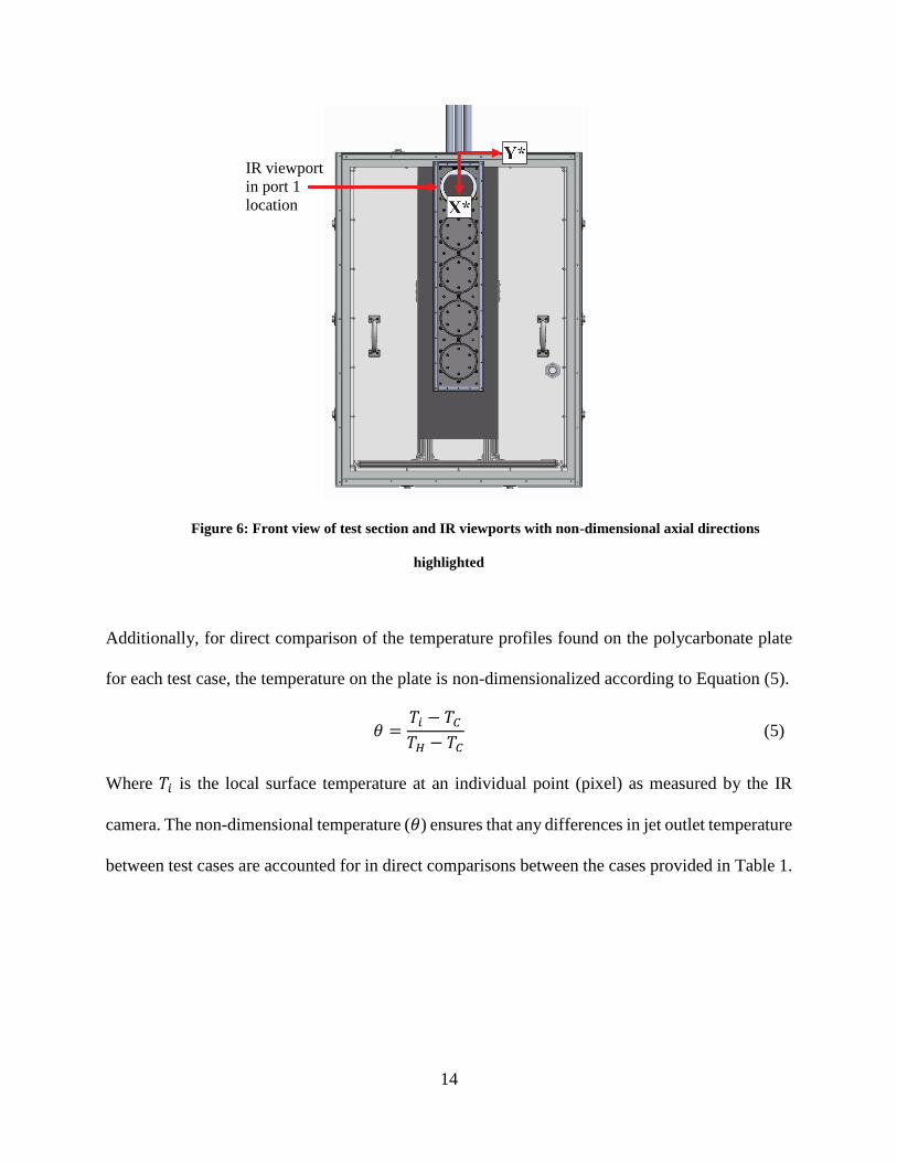
Figure 6: Front view of test section and IR viewports with non-dimensional axial directions

highlighted ........................................................................................................................ 14

ix

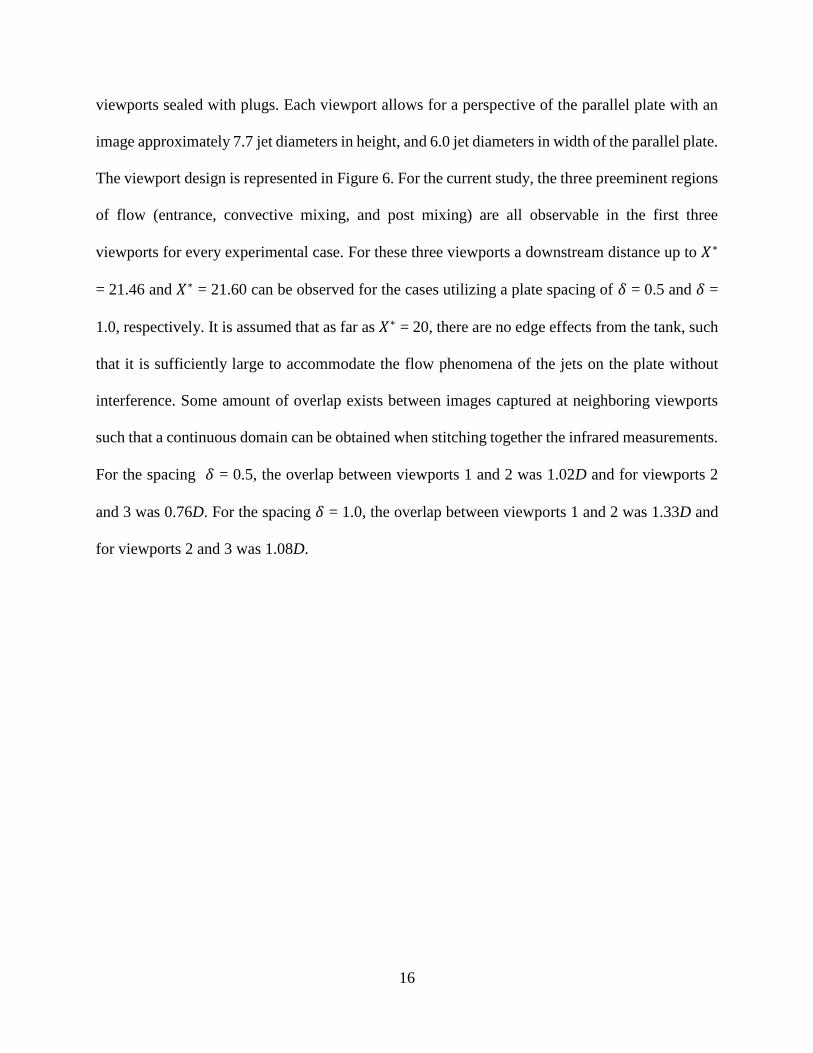
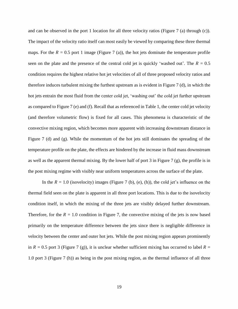
Figure 7: Contours of triple jet-induced temperature fields across parallel wall for ∆𝑇 = 44.4°C

and 𝛿 = 0.5. Approximate size of each image is 13.4 cm x 17.1 cm (a) 𝑅 = 0.5 port 1 (b) 𝑅

= 1.0 port 1 (c) 𝑅 = 1.5 port 1 (d) 𝑅 = 0.5 port 2 (e) 𝑅 = 1.0 port 2 (f) 𝑅 = 1.5 port 2 (g) 𝑅

= 0.5 port 3 (h) 𝑅 = 1.0 port 3 (i) 𝑅 = 1.5 port 3 ............................................................... 18

Figure 8: Time-averaged temperature contours and corresponding temperature fluctuations from

Kimura et al. [11] .............................................................................................................. 21

Figure 9: (a) Case 4, port 1 temperature field with imposed line traces (b) Case 4, port 1

polycarbonate plate line trace surface temperatures ......................................................... 23

Figure 10: Total uncertainty range for 𝑋∗=2 line trace of case 4 ................................................. 28

Figure 11: Line temperature profiles with fixed ∆𝑇 = 44.4°C and 𝛿 = 0.5 .................................. 30

Figure 12: Temperature difference and plate spacing comparison in three characteristic flow

regions ............................................................................................................................... 34

Figure 13: Case 10, port 1 temperature field with imposed line traces ........................................ 35

x

Figure 14: Peak temperature location for each line temperature trace with imposed hot jet center

line..................................................................................................................................... 38

xi

PREFACE

This research is being performed using funding received from the DOE Office of Nuclear Energy's

Nuclear Energy University Programs.

xii

NOMENCLATURE

𝑋 axial direction

𝜐 degrees of freedom of fit

𝐷 diameter (of jet unless otherwise noted)

𝜖 emissivity

휀 error

𝐿 length

𝑋∗ non-dimensional axial direction

𝑌∗ non-dimensional radial direction

𝜃 non-dimensional temperature

𝑁 number of sets of measurements

𝛿 plate spacing

𝑆 scaled jet spacing

𝑠 standard deviation

𝑡 student’s t-distribution

𝑌 radial direction

𝑅𝑒 Reynolds number

𝑇 temperature

∆𝑇 temperature difference between cold and hot jet outlets

xiii

𝑈 uncertainty

𝑉 velocity

𝑅 velocity ratio

SUBSCRIPTS

𝑎𝑠𝑦𝑚 asymmetric

𝑐𝑎𝑙 calibration

𝐶 cold jet

𝑐𝑒𝑙𝑙 hexagonal honeycomb cell

𝐻 hot jet

ℎ𝑐 honeycomb

ℎ𝑦𝑑 hydraulic

𝐿𝐻𝑆 left-hand side

𝑚 mean

𝑜 outlet

𝑝𝑟𝑒𝑐 precision

𝑟𝑒𝑝 repeatability

𝑟𝑒𝑠 resolution

xiv

𝑅𝐻𝑆 right-hand side

𝑡𝑜𝑡 total

1

1.0 INTRODUCTION

The turbulent mixing of hot and cold fluids experience thermal fluctuations within the mixing

region. These temperature fluctuations are transmitted to the supporting structure and can cause

severe high cycle thermal fatigue over the course of a component’s operational lifetime, a process

also known as thermal striping. In both existing and next generation nuclear reactor designs, this

has been and continues to be a major focus of study. Over the course of a reactor’s lifespan, the

effects of thermal striping can jeopardize the structural integrity of the nuclear reactor core.

Thermal striping is a particular concern in the Generation IV very high temperature gas reactor

(VHTR), which employs helium as a coolant. Using a gas for the coolant enables natural

convective cooling under accident scenarios, but can alternatively produce higher thermal

fluctuations than modern pressurized water reactors (PWRs). The helium extracts heat throughout

the core before mixing in the lower plenum in a confined series of jets. These jets enter the lower

plenum at different temperatures (on the order of 300˚C [1, 2]) caused by the non-uniform heat

generation in the reactor core. In addition, the inability to evenly distribute the flow through the

hundreds of coolant channels produces a range of jet velocities, which further complicates the

mixing.

The issue of thermal striping in nuclear reactors was first identified as a major cause of

structural fatigue in the early 1980s [3-5]. Lloyd and Wood [5] first presented the issue in their

analysis on the initiation and subsequent propagation of surface cracks in a stainless steel section

2

subjected to high frequency thermal shocks. Thermal shocking is defined as the condition in which

the surface temperature change has occurred before the effects have significantly penetrated into

the component wall [4]. With repeated thermal shocks, the thermal striping experienced by internal

wall components becomes more severe over time. A standard approach to quantify the underlying

flow physics and loading during thermal striping is to study arrays of parallel jets, which also

serves as the basis for this investigation.

A common configuration seen in previous experimental and numerical investigations is

that of a parallel triple jet. This has been studied for “quasi-free jets” (i.e., where solid walls or

boundaries are far removed from the jets), as well as for thermal and fluid interactions with solid

components in close proximity. Tokuhiro and Kimura [6] conducted experiments using a triple

slot jet configuration including a central cold jet (non-buoyant) and a hot jet on either side

(considered buoyant) with water as the working fluid. They compared the behavior to that of

reference single jet. Three regions of flow were studied: (1) the “entrance” region where

temperature was considered constant (negligible increase in cold jet temperature or decrease in hot

jet temperature), (2) the “convective mixing” area where the temperature increase/decrease has

become significant, and (3) the “post mixing” region where the temperature assumes an

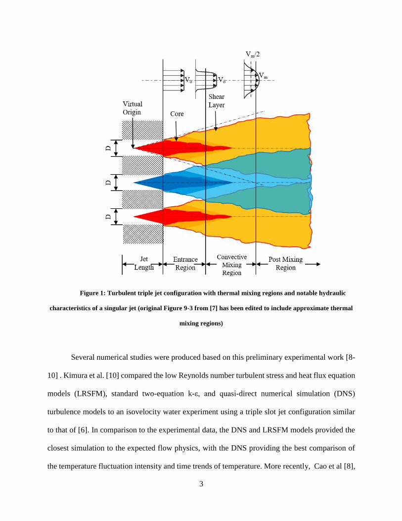
asymptotically decreasing trend [6]. A visual representation of the general triple jet configuration

and these corresponding thermal regions is provided in Figure 1, which was edited from the

original figure of a submerged turbulent jet from [7]. For reference, the notable features of an

individual jet and expected velocity profiles (at approximate downstream lengths) are also

included, however it should be noted that sufficiently far downstream, the three jets form a singular

composite jet.

3

Figure 1: Turbulent triple jet configuration with thermal mixing regions and notable hydraulic

characteristics of a singular jet (original Figure 9-3 from [7] has been edited to include approximate thermal

mixing regions)

Several numerical studies were produced based on this preliminary experimental work [8-

10] . Kimura et al. [10] compared the low Reynolds number turbulent stress and heat flux equation

models (LRSFM), standard two-equation k-ε, and quasi-direct numerical simulation (DNS)

turbulence models to an isovelocity water experiment using a triple slot jet configuration similar

to that of [6]. In comparison to the experimental data, the DNS and LRSFM models provided the

closest simulation to the expected flow physics, with the DNS providing the best comparison of

the temperature fluctuation intensity and time trends of temperature. More recently, Cao et al [8],

4

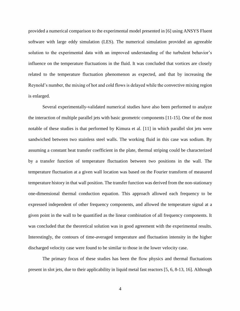
provided a numerical comparison to the experimental model presented in [6] using ANSYS Fluent

software with large eddy simulation (LES). The numerical simulation provided an agreeable

solution to the experimental data with an improved understanding of the turbulent behavior’s

influence on the temperature fluctuations in the fluid. It was concluded that vortices are closely

related to the temperature fluctuation phenomenon as expected, and that by increasing the

Reynold’s number, the mixing of hot and cold flows is delayed while the convective mixing region

is enlarged.

Several experimentally-validated numerical studies have also been performed to analyze

the interaction of multiple parallel jets with basic geometric components [11-15]. One of the most

notable of these studies is that performed by Kimura et al. [11] in which parallel slot jets were

sandwiched between two stainless steel walls. The working fluid in this case was sodium. By

assuming a constant heat transfer coefficient in the plate, thermal striping could be characterized

by a transfer function of temperature fluctuation between two positions in the wall. The

temperature fluctuation at a given wall location was based on the Fourier transform of measured

temperature history in that wall position. The transfer function was derived from the non-stationary

one-dimensional thermal conduction equation. This approach allowed each frequency to be

expressed independent of other frequency components, and allowed the temperature signal at a

given point in the wall to be quantified as the linear combination of all frequency components. It

was concluded that the theoretical solution was in good agreement with the experimental results.

Interestingly, the contours of time-averaged temperature and fluctuation intensity in the higher

discharged velocity case were found to be similar to those in the lower velocity case.

The primary focus of these studies has been the flow physics and thermal fluctuations

present in slot jets, due to their applicability in liquid metal fast reactors [5, 6, 8-13, 16]. Although

5

qualitatively similar, round jets exhibit fundamentally different flow physics (e.g., jet decay and

spreading rate as shown in [17], [18]) and are not just of interest in the prismatic VHTR lower

plenum, but are encountered in other applications, including flame base topology in combustion

applications [19], the influence of acoustic excitation on the heat transfer and flow behavior of a

round impinging jet [20], and electronic cooling with the use of synthetic round jet impingement

[21]. While these experimental studies provide a better understanding of the underlying flow

physics of a singular round jet in various applications, the lack of experimental and numerical

work done with multiple turbulent round jets leaves more analysis to be desired. This is of

particular concern regarding the jet outlets found in the lower plenum of the prismatic VHTR.

For primary validation efforts with respect to thermal loading in the plate, the time

averaged thermal signatures are required. The subject of multiple turbulent circular jets is of great

significance in the study of the VHTR lower plenum for several different cases. Several

experimental studies have been conducted regarding flow visualization of VHTR components

subject to jet impingement including [22-24]. Likewise, experimental-validation for computational

modeling of accident scenarios of the VHTR have been examined [25, 26]. Although these and

other studies provide insight into unique flow conditions and characteristics, a slightly different

approach is also worthwhile. For validation purposes, the planned experiments should focus on

relevant, yet simplistic configurations, rather than try to include all the complexities of the actual

application. Without a fundamentals-based experiment, it becomes difficult to validate

computational models and their underlying assumptions since the geometric requirements of the

mesh could drastically increase the computational cost beyond desired levels. Therefore, the

secondary contribution of the current work is to provide such data for a triple parallel round jet

near a solid wall.

6

2.0 EXPERIMENT

2.1 EXPERIMENTAL FACILITY

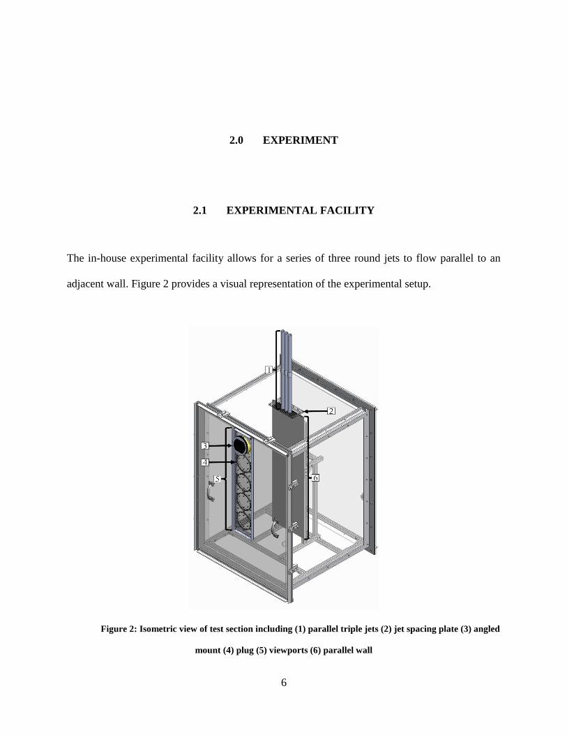
The in-house experimental facility allows for a series of three round jets to flow parallel to an

adjacent wall. Figure 2 provides a visual representation of the experimental setup.

Figure 2: Isometric view of test section including (1) parallel triple jets (2) jet spacing plate (3) angled

mount (4) plug (5) viewports (6) parallel wall

7

The facility includes a 73.7 cm x 76.2 cm x 106.7 cm enclosed test section with (as

referenced in Figure 2) three parallel round jets whose outlets are located on the top surface of the

test section which are fixed to the appropriate jet spacing at the inlet of the test section via a jet

spacing plate. The front surface of the test section incorporates an angled mount, which holds a

broadband crystal lens, and four polycarbonate plugs all housed in five separate viewport locations.

Inside the test section is the parallel wall of dimensions 27.9 cm x 96.5 cm x 0.9 cm which is fixed

via a structural support frame. The parallel wall is composed of polycarbonate and is painted with

Krylon 1602 paint having an emissivity (ϵ) of 0.95 [27]. The polycarbonate plate has a melting

temperature of 155°C and a thermal conductivity of 0.19 W m-1 K-1, which minimizes the thermal

smearing (lateral conduction) and enables a clear thermal signature to be revealed on the surface.

The use of these experimental components is expanded in the proceeding sections in regards to

measuring the surface temperature on the parallel wall. The three parallel jets are fixed vertically

via a structural support frame and are connected to a corresponding external temperature and flow

control skid. A process flow diagram of the external temperature and flow control skid is included

in Figure 3.

8

Figure 3: Process flow diagram of external temperature and flow control skid

The temperature and flow control skid includes two separate heaters for the two outermost

jet lines and a heat exchanger (cooled with a secondary water line) for the center jet line with flow

for all three lines produced by a blower. The blower is capable of motivating 7.08 m3/s at an

operating pressure of 2.04×104 Pa. The test section’s outer support frame includes rubber feet to

dampen any type of unwanted vibrational response from the surrounding environment. At the

bottom of the test section, a 5.08 cm line allows air to exit the facility. The exit line at the bottom

of the test section returns to the temperature and flow control skid, forming a closed loop. An

additional system heat exchanger is included to regulate unwanted increases in jet temperatures

from downstream mixing and re-entry of the flow in the blower.

The flow control skid utilizes air as the working fluid. The volumetric flow of the individual

jets are held constant by the temperature and flow control skid’s automated valves after the jet

temperatures reach steady state, which for the current study, provides a worst case uncertainty of

+/-1.6%. The jet outlet conditions are also of considerable interest, for both the current

9

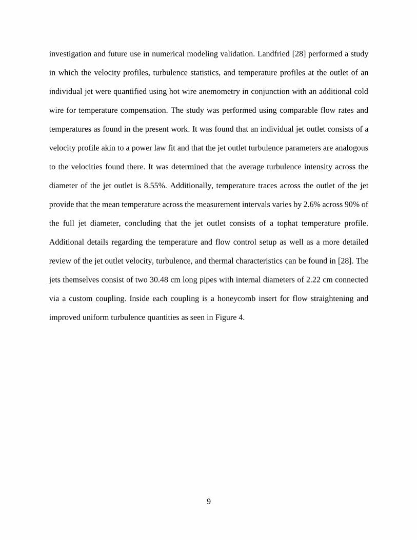
investigation and future use in numerical modeling validation. Landfried [28] performed a study

in which the velocity profiles, turbulence statistics, and temperature profiles at the outlet of an

individual jet were quantified using hot wire anemometry in conjunction with an additional cold

wire for temperature compensation. The study was performed using comparable flow rates and

temperatures as found in the present work. It was found that an individual jet outlet consists of a

velocity profile akin to a power law fit and that the jet outlet turbulence parameters are analogous

to the velocities found there. It was determined that the average turbulence intensity across the

diameter of the jet outlet is 8.55%. Additionally, temperature traces across the outlet of the jet

provide that the mean temperature across the measurement intervals varies by 2.6% across 90% of

the full jet diameter, concluding that the jet outlet consists of a tophat temperature profile.

Additional details regarding the temperature and flow control setup as well as a more detailed

review of the jet outlet velocity, turbulence, and thermal characteristics can be found in [28]. The

jets themselves consist of two 30.48 cm long pipes with internal diameters of 2.22 cm connected

via a custom coupling. Inside each coupling is a honeycomb insert for flow straightening and

improved uniform turbulence quantities as seen in Figure 4.

10

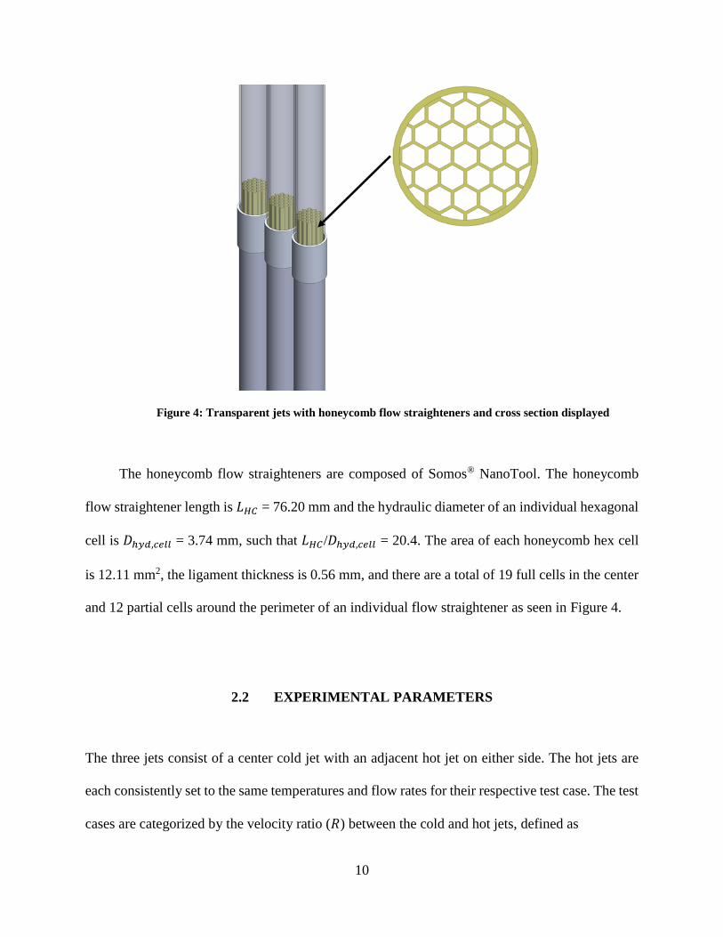
Figure 4: Transparent jets with honeycomb flow straighteners and cross section displayed

The honeycomb flow straighteners are composed of Somos® NanoTool. The honeycomb

flow straightener length is 𝐿𝐻𝐶 = 76.20 mm and the hydraulic diameter of an individual hexagonal

cell is 𝐷ℎ𝑦𝑑,𝑐𝑒𝑙𝑙 = 3.74 mm, such that 𝐿𝐻𝐶/𝐷ℎ𝑦𝑑,𝑐𝑒𝑙𝑙 = 20.4. The area of each honeycomb hex cell

is 12.11 mm2, the ligament thickness is 0.56 mm, and there are a total of 19 full cells in the center

and 12 partial cells around the perimeter of an individual flow straightener as seen in Figure 4.

2.2 EXPERIMENTAL PARAMETERS

The three jets consist of a center cold jet with an adjacent hot jet on either side. The hot jets are

each consistently set to the same temperatures and flow rates for their respective test case. The test

cases are categorized by the velocity ratio (𝑅) between the cold and hot jets, defined as

11

𝑅 =𝑉𝐶

𝑉𝐻 (1)

Where 𝑉𝐶 is the velocity of the cold jet and 𝑉𝐻 is the velocity of each hot jet. Each velocity

ratio 𝑅 is subject to a temperature difference between the jets, defined as

∆𝑇 = 𝑇𝐻 − 𝑇𝐶 (2)

Where 𝑇𝐻 is the outlet temperature of the hot jets and 𝑇𝐶 is the outlet temperature of the

center cold jet. For this experimental study, the two prescribed temperature differences between

the jets are ∆𝑇 =33.3˚C and ∆𝑇 =44.4˚C. Additionally, two physical spacings are defined. The

plate spacing, 𝛿 is the separation distance between the plate surface and the axial centerline of the

three jets. For this experimental study, two spacings are considered: one where the plate surface is

fixed directly tangent to the outlet of the jets (𝛿 = 0.5) and one jet diameter away (𝛿 = 1.0). The

jet spacing, 𝑆, is the relative inline distance of the jet centers from one another and is based on a

scaled mock-up of the General Atomics gas turbine modular helium reactor (GT-MHR) [29]. The

scaled jet spacing for this study is fixed 𝑆 = 3.13 cm. It should be noted that the General Atomics

GT-MHR consists of a prismatic core design in which the outlets of the jets in the lower plenum

are in hexagonal configurations. While the prismatic core design consists of staggered arrays of

jets in relative 120˚ triangles, the more fundamental 180˚ (planar) triple jet configuration used here

provides a better preliminary analysis to compare against previous non-isothermal triple jet data

as discussed prior, and to offer experimental conditions more easily used for computational

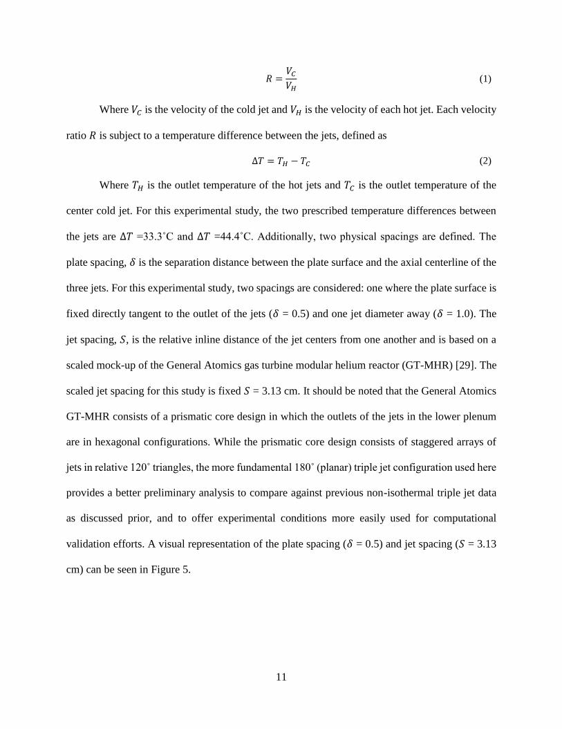
validation efforts. A visual representation of the plate spacing (𝛿 = 0.5) and jet spacing (𝑆 = 3.13

cm) can be seen in Figure 5.

12

Figure 5: Top view of triple jet test section and confining wall with highlighted spacing parameters

The outlet velocities of the individual jets were determined according to their

corresponding volumetric flow rates (governed by the automated valves) and the diameter of the

jets. The Reynold’s numbers for the jet outlets were calculated based on these velocities and the

corresponding temperature dependent fluid properties as a function of the jet outlet temperatures.

With the jet outlet velocities and temperatures known, the velocity ratio and temperature difference

are calculated with ease. The test cases are presented in Table 1.

13

Table 1: Experimental conditions

Case name Hot jet Cold jet (center) R ∆T (˚C) δ

VH

(m/s)

ReH TH (˚C)

VC

(m/s)

ReC TC (˚C)

Case 1 15.63 1.79x104 62.1 7.75 1.07x104 28.8 0.50 33.3 0.5

Case 2 7.75 8.88x103 61.6 7.75 1.08x104 28.2 1.00 33.4 0.5

Case 3 5.12 5.89x103 61.1 7.75 1.08x104 27.5 1.51 33.6 0.5

Case 4 15.63 1.67x104 75.8 7.75 1.05x104 31.3 0.50 44.5 0.5

Case 5 7.75 8.24x103 76.8 7.75 1.05x104 32.0 1.00 44.8 0.5

Case 6 5.12 5.51x103 74.2 7.75 1.07x104 29.5 1.51 44.7 0.5

Case 7 15.63 1.76x104 65.6 7.75 1.05x104 32.7 0.50 32.9 1.0

Case 8 7.75 8.76x103 64.4 7.75 1.06x104 31.0 1.00 33.4 1.0

Case 9 5.12 5.86x103 61.9 7.75 1.07x104 28.4 1.51 33.4 1.0

Case 10 15.63 1.63x104 80.4 7.75 1.03x104 36.2 0.50 44.3 1.0

Case 11 7.75 8.18x103 78.2 7.75 1.04x104 33.8 1.00 44.3 1.0

Case 12 5.12 5.47x103 75.7 7.75 1.05x104 31.3 1.51 44.4 1.0

For convenience, the velocity ratio, 𝑅 will be referred to in terms of its nominal value for the

analysis to follow, i.e. 𝑅 ≈ 0.5, 1.0, or 1.5. Several non-dimensional parameters are incorporated

as well. The non-dimensional axial direction 𝑋∗ is defined as

𝑋∗ =𝑋

𝐷 (3)

Where 𝑋 is the downstream distance from the outlet of the cold jet and D is the diameter of an

individual jet. The non-dimensional radial direction 𝑌∗ is defined as

𝑌∗ =𝑌

𝑆 (4)

Where 𝑌 is the inline distance along the jet outlets from the cold jet center and 𝑆 is the jet spacing

as seen previously in Figure 5. A visual representation of the non-dimensionalized directions 𝑋∗

and 𝑌∗ is found in Figure 6.

14

Figure 6: Front view of test section and IR viewports with non-dimensional axial directions

highlighted

Additionally, for direct comparison of the temperature profiles found on the polycarbonate plate

for each test case, the temperature on the plate is non-dimensionalized according to Equation (5).

𝜃 =𝑇𝑖 − 𝑇𝐶

𝑇𝐻 − 𝑇𝐶 (5)

Where 𝑇𝑖 is the local surface temperature at an individual point (pixel) as measured by the IR

camera. The non-dimensional temperature (𝜃) ensures that any differences in jet outlet temperature

between test cases are accounted for in direct comparisons between the cases provided in Table 1.

IR viewport

in port 1

location

15

2.3 EXPERIMENTAL METHODS

The jet outlet temperatures are determined experimentally by placing a type-T thermocouple at the

outlet of each jet. It is assumed that the thermocouples are sufficiently small such that they did not

interfere with the velocity profiles at the outlet of the jets. The thermocouples were calibrated using

an OMEGA hot point® Dry Block Probe Calibrator and reference thermistor with an accuracy of

+/- 0.156 °C at a maximum operating temperature of 130 °C. A FLIR SC5000 IR camera with a

resolution of +/- 1.0 °C for absolute temperatures is used to acquire the temperature signatures

induced by the jets on the parallel plate. The IR camera was calibrated with a blackbody emitter

(Infrared Systems Development model IR-2106 radiation source and model IR-301 digital

temperature controller) with an accuracy of +/- 0.2 °C at a maximum operating temperature of 150

°C. The accuracy of the measurement equipment is incorporated into the overall uncertainty in 𝜃,

and is evaluated in Section 3.2.

The test section walls are composed of 1.11 cm thick polycarbonate and have poor infrared

transmittance in the wavelength spectrum of the IR camera (2.1-5.1 μm). For this reason, a FLIR

4-inch Infrared (IR) viewport (model IRW-4C) is incorporated, which includes a broadband crystal

lens with a maximum operating temperature of 260°C. The camera is placed 55.88 cm from the

front surface of the parallel plate enabling a resolution of 0.5 mm. To avoid reflection of the camera

on the IR window, a custom mount is built which ensures that the window axis and camera axis

are offset by 10°. Additionally, a shroud is placed between the camera lens and the viewport which

eliminates any incident thermal radiation. Accommodation exists for 5 viewports on the front

surface of the test section with a center-to-center distance of 15.24 cm for each adjacent viewport.

The angled mount and IR window can be placed in any of these five viewports with the remaining

16

viewports sealed with plugs. Each viewport allows for a perspective of the parallel plate with an

image approximately 7.7 jet diameters in height, and 6.0 jet diameters in width of the parallel plate.

The viewport design is represented in Figure 6. For the current study, the three preeminent regions

of flow (entrance, convective mixing, and post mixing) are all observable in the first three

viewports for every experimental case. For these three viewports a downstream distance up to 𝑋∗

= 21.46 and 𝑋∗ = 21.60 can be observed for the cases utilizing a plate spacing of 𝛿 = 0.5 and 𝛿 =

1.0, respectively. It is assumed that as far as 𝑋∗ = 20, there are no edge effects from the tank, such

that it is sufficiently large to accommodate the flow phenomena of the jets on the plate without

interference. Some amount of overlap exists between images captured at neighboring viewports

such that a continuous domain can be obtained when stitching together the infrared measurements.

For the spacing 𝛿 = 0.5, the overlap between viewports 1 and 2 was 1.02D and for viewports 2

and 3 was 0.76D. For the spacing 𝛿 = 1.0, the overlap between viewports 1 and 2 was 1.33D and

for viewports 2 and 3 was 1.08D.

17

3.0 RESULTS

3.1 TEMPERATURE PROFILE CASE STUDY

The temperature profiles captured by the IR camera for cases 4-6 in Table 1 are presented in Figure

7. Cases included in Figure 7 are selected for having the highest temperature difference (∆𝑇 =

44.4˚C) at the closest plate spacing (𝛿 = 0.5) and therefore reveal the highest temperature contrasts,

and most easily illustrate the mixing patterns. The temperature scaling of each figure is held

constant to enable qualitative and quantitative comparisons between experimental images.

18

(a) (b) (c)

(d) (e) (f)

(g) (h) (i)

Figure 7: Contours of triple jet-induced temperature fields across parallel wall for T = 44.4C and

= 0.5. Approximate size of each image is 13.4 cm x 17.1 cm (a) 𝑹 = 0.5 port 1 (b) 𝑹 = 1.0 port 1 (c) 𝑹 = 1.5 port

1 (d) 𝑹 = 0.5 port 2 (e) 𝑹 = 1.0 port 2 (f) 𝑹 = 1.5 port 2 (g) 𝑹 = 0.5 port 3 (h) 𝑹 = 1.0 port 3 (i) 𝑹 = 1.5 port 3

It should be noted that the other case studies provided similar contours and are therefore

omitted, but the data are included in the analysis that follows. From Figure 7, the most visible

influence of the unique jet outlet temperatures on the surface temperature of the polycarbonate

plate is in the 𝑅 = 1.5 port 1 temperature field (Figure 7 (c)). The results show the presence of the

jets is immediately felt by the plate with high temperature contrasts near the jet nozzles. This

region, where negligible change in temperature has occurred, is considered the entrance region,

19

and can be observed in the port 1 location for all three velocity ratios (Figure 7 (a) through (c)).

The impact of the velocity ratio itself can most easily be viewed by comparing these three thermal

maps. For the 𝑅 = 0.5 port 1 image (Figure 7 (a)), the hot jets dominate the temperature profile

seen on the plate and the presence of the central cold jet is quickly ‘washed out’. The 𝑅 = 0.5

condition requires the highest relative hot jet velocities of all of three proposed velocity ratios and

therefore induces turbulent mixing the furthest upstream as is evident in Figure 7 (d), in which the

hot jets entrain the most fluid from the center cold jet, ‘washing out’ the cold jet further upstream

as compared to Figure 7 (e) and (f). Recall that as referenced in Table 1, the center cold jet velocity

(and therefore volumetric flow) is fixed for all cases. This phenomena is characteristic of the

convective mixing region, which becomes more apparent with increasing downstream distance in

Figure 7 (d) and (g). While the momentum of the hot jets still dominates the spreading of the

temperature profile on the plate, the effects are hindered by the increase in fluid mass downstream

as well as the apparent thermal mixing. By the lower half of port 3 in Figure 7 (g), the profile is in

the post mixing regime with visibly near uniform temperatures across the surface of the plate.

In the 𝑅 = 1.0 (isovelocity) images (Figure 7 (b), (e), (h)), the cold jet’s influence on the

thermal field seen on the plate is apparent in all three port locations. This is due to the isovelocity

condition itself, in which the mixing of the three jets are visibly delayed further downstream.

Therefore, for the 𝑅 = 1.0 condition in Figure 7, the convective mixing of the jets is now based

primarily on the temperature difference between the jets since there is negligible difference in

velocity between the center and outer hot jets. While the post mixing region appears prominently

in 𝑅 = 0.5 port 3 (Figure 7 (g)), it is unclear whether sufficient mixing has occurred to label 𝑅 =

1.0 port 3 (Figure 7 (h)) as being in the post mixing region, as the thermal influence of all three

20

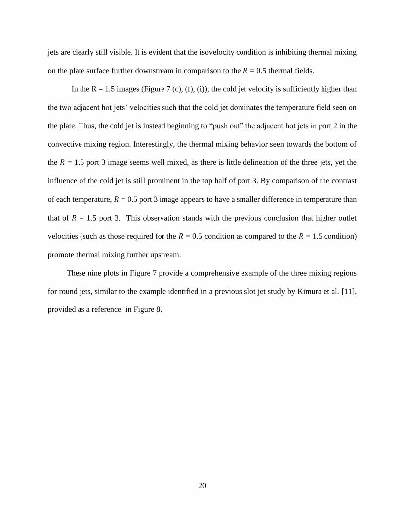
jets are clearly still visible. It is evident that the isovelocity condition is inhibiting thermal mixing

on the plate surface further downstream in comparison to the 𝑅 = 0.5 thermal fields.

In the R = 1.5 images (Figure 7 (c), (f), (i)), the cold jet velocity is sufficiently higher than

the two adjacent hot jets’ velocities such that the cold jet dominates the temperature field seen on

the plate. Thus, the cold jet is instead beginning to “push out” the adjacent hot jets in port 2 in the

convective mixing region. Interestingly, the thermal mixing behavior seen towards the bottom of

the 𝑅 = 1.5 port 3 image seems well mixed, as there is little delineation of the three jets, yet the

influence of the cold jet is still prominent in the top half of port 3. By comparison of the contrast

of each temperature, 𝑅 = 0.5 port 3 image appears to have a smaller difference in temperature than

that of 𝑅 = 1.5 port 3. This observation stands with the previous conclusion that higher outlet

velocities (such as those required for the 𝑅 = 0.5 condition as compared to the 𝑅 = 1.5 condition)

promote thermal mixing further upstream.

These nine plots in Figure 7 provide a comprehensive example of the three mixing regions

for round jets, similar to the example identified in a previous slot jet study by Kimura et al. [11],

provided as a reference in Figure 8.

21

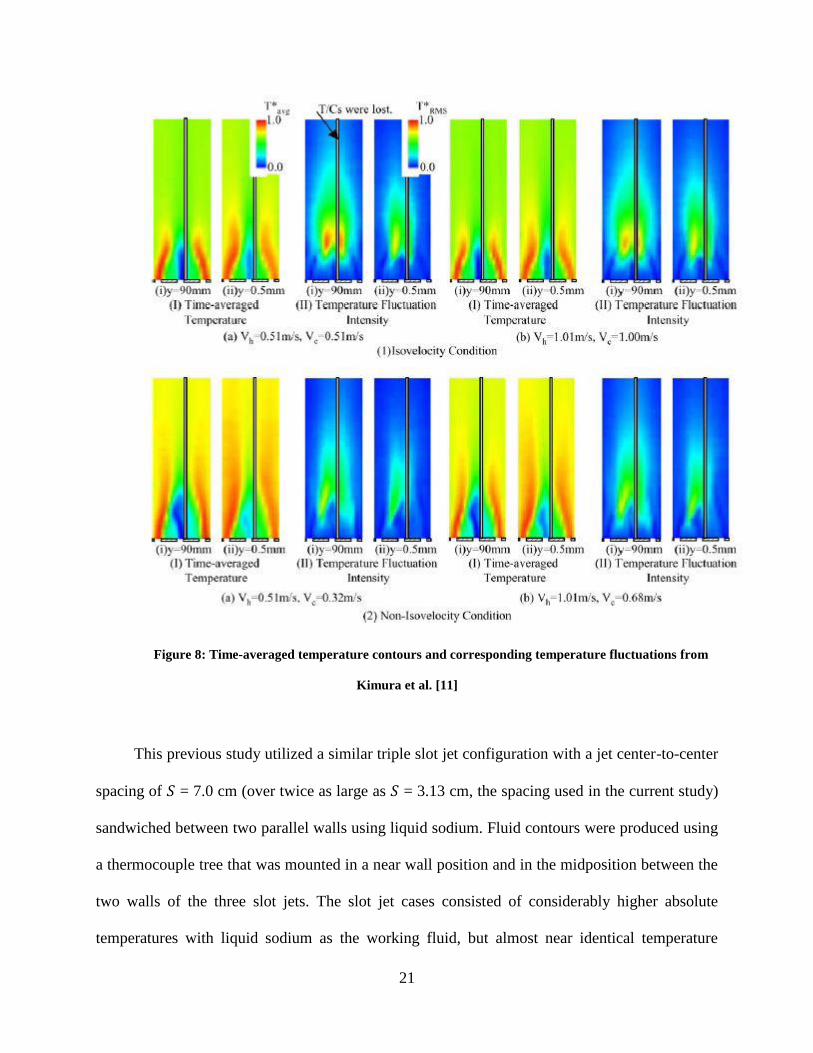
Figure 8: Time-averaged temperature contours and corresponding temperature fluctuations from

Kimura et al. [11]

This previous study utilized a similar triple slot jet configuration with a jet center-to-center

spacing of 𝑆 = 7.0 cm (over twice as large as 𝑆 = 3.13 cm, the spacing used in the current study)

sandwiched between two parallel walls using liquid sodium. Fluid contours were produced using

a thermocouple tree that was mounted in a near wall position and in the midposition between the

two walls of the three slot jets. The slot jet cases consisted of considerably higher absolute

temperatures with liquid sodium as the working fluid, but almost near identical temperature

22

differences between the jets [11]. The use of water and air as substitutes for liquid sodium has

been outlined by Moriya and Ohshima [30] for simulating the characteristics of temperature

fluctuation due to turbulent mixing. Since the contours provided by Kimura et al. are time-

averaged, their qualitative comparison to the steady-state contours provided in Figure 7 is justified.

The geometry of the slot and round jet outlets induce different thermal profiles in the entrance

region, however the majority of the difference in the downstream mixing is attributed to the

spacing between the jets being more than double that of the current study. The contours of the

round jets’ thermal interactions with the surface of the plate show much wider spreading in the 𝑌∗-

direction in contrast to the relatively narrow and more distinct shape seen by the fluid interactions

of the slot jets.

3.2 TEMPERATURE LINE TRACE COMPARISON

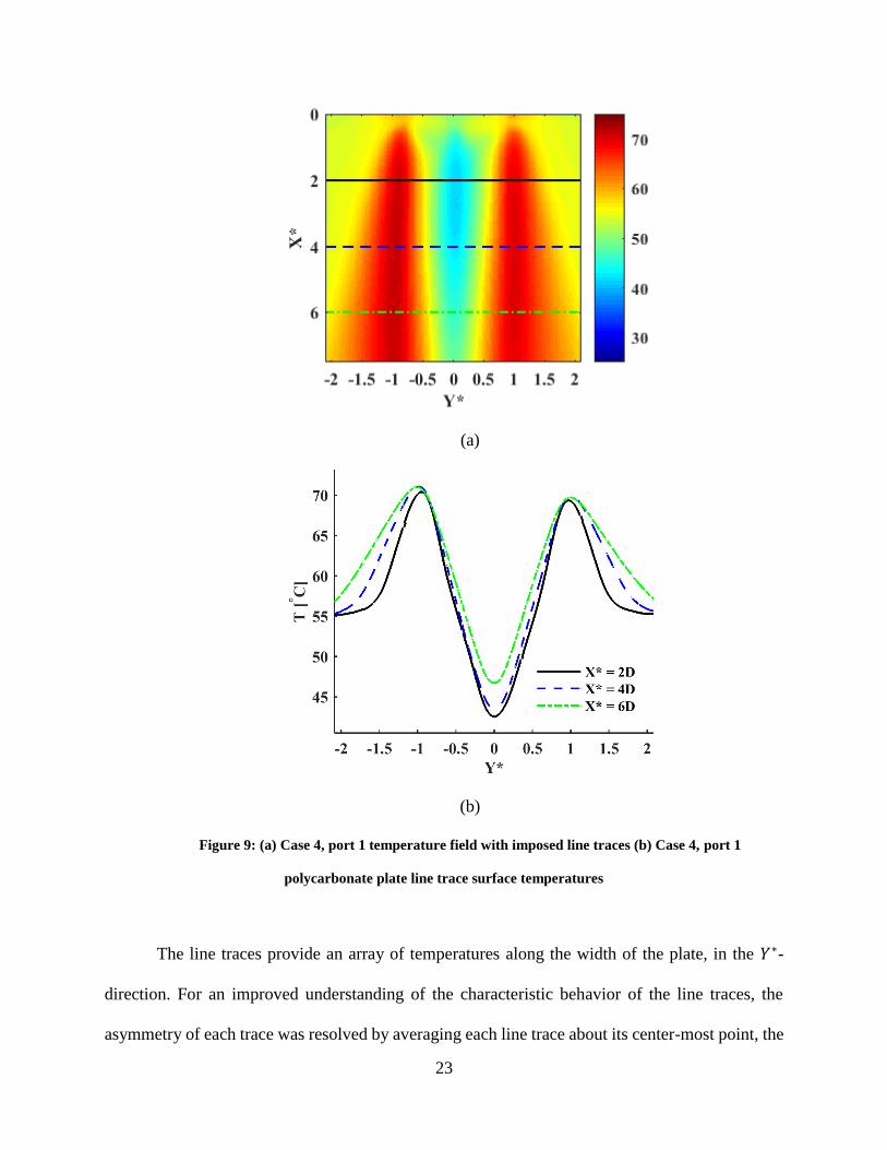
Line traces of the temperature data were utilized in 𝑋∗= 2 increments in the downstream 𝑋∗-

direction for each temperature field. A total of 10 line traces were evaluated accounting for a range

of 𝑋∗ values between 𝑋∗= 2-20 downstream. As an example, a visualization of the line traces and

the corresponding temperatures are provided in Figure 9 for port 1 of case 4.

23

(a)

(b)

Figure 9: (a) Case 4, port 1 temperature field with imposed line traces (b) Case 4, port 1

polycarbonate plate line trace surface temperatures

The line traces provide an array of temperatures along the width of the plate, in the 𝑌∗-

direction. For an improved understanding of the characteristic behavior of the line traces, the

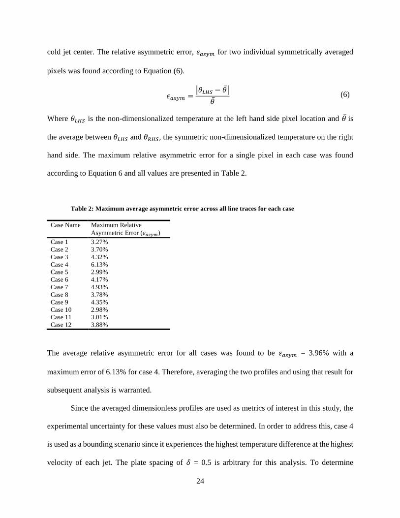
asymmetry of each trace was resolved by averaging each line trace about its center-most point, the

24

cold jet center. The relative asymmetric error, 휀𝑎𝑠𝑦𝑚 for two individual symmetrically averaged

pixels was found according to Equation (6).

𝜖𝑎𝑠𝑦𝑚 =|𝜃𝐿𝐻𝑆 − �̅�|

�̅� (6)

Where 𝜃𝐿𝐻𝑆 is the non-dimensionalized temperature at the left hand side pixel location and �̅� is

the average between 𝜃𝐿𝐻𝑆 and 𝜃𝑅𝐻𝑆, the symmetric non-dimensionalized temperature on the right

hand side. The maximum relative asymmetric error for a single pixel in each case was found

according to Equation 6 and all values are presented in Table 2.

Table 2: Maximum average asymmetric error across all line traces for each case

Case Name Maximum Relative

Asymmetric Error (휀𝑎𝑠𝑦𝑚)

Case 1 3.27%

Case 2 3.70%

Case 3 4.32%

Case 4 6.13%

Case 5 2.99%

Case 6 4.17%

Case 7 4.93%

Case 8 3.78%

Case 9 4.35%

Case 10 2.98%

Case 11 3.01%

Case 12 3.88%

The average relative asymmetric error for all cases was found to be 휀𝑎𝑠𝑦𝑚 = 3.96% with a

maximum error of 6.13% for case 4. Therefore, averaging the two profiles and using that result for

subsequent analysis is warranted.

Since the averaged dimensionless profiles are used as metrics of interest in this study, the

experimental uncertainty for these values must also be determined. In order to address this, case 4

is used as a bounding scenario since it experiences the highest temperature difference at the highest

velocity of each jet. The plate spacing of 𝛿 = 0.5 is arbitrary for this analysis. To determine

25

repeatability, a total of five tests with these identical experimental settings were run over the course

of 10 days. Although the temperature of the room was found to fluctuate throughout the day, which

caused some amount of variation in absolute temperatures, the dimensionless form of the

temperature was found to show excellent repeatability from day to day. The repeatability error in

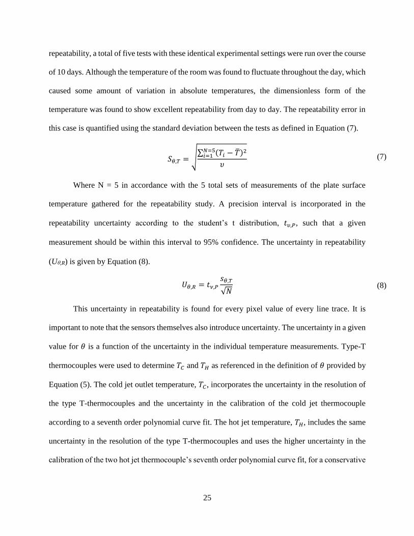
this case is quantified using the standard deviation between the tests as defined in Equation (7).

𝑆𝜃,𝑇 = √∑ (𝑇𝑖 − �̅�)2𝑁=5

𝑖=1

𝜐 (7)

Where N = 5 in accordance with the 5 total sets of measurements of the plate surface

temperature gathered for the repeatability study. A precision interval is incorporated in the

repeatability uncertainty according to the student’s t distribution, 𝑡𝜐,𝑃, such that a given

measurement should be within this interval to 95% confidence. The uncertainty in repeatability

(U,R) is given by Equation (8).

𝑈𝜃,𝑅 = 𝑡𝜈,𝑃

𝑠𝜃,𝑇

√𝑁 (8)

This uncertainty in repeatability is found for every pixel value of every line trace. It is

important to note that the sensors themselves also introduce uncertainty. The uncertainty in a given

value for 𝜃 is a function of the uncertainty in the individual temperature measurements. Type-T

thermocouples were used to determine 𝑇𝐶 and 𝑇𝐻 as referenced in the definition of 𝜃 provided by

Equation (5). The cold jet outlet temperature, 𝑇𝐶, incorporates the uncertainty in the resolution of

the type T-thermocouples and the uncertainty in the calibration of the cold jet thermocouple

according to a seventh order polynomial curve fit. The hot jet temperature, 𝑇𝐻, includes the same

uncertainty in the resolution of the type T-thermocouples and uses the higher uncertainty in the

calibration of the two hot jet thermocouple’s seventh order polynomial curve fit, for a conservative

26

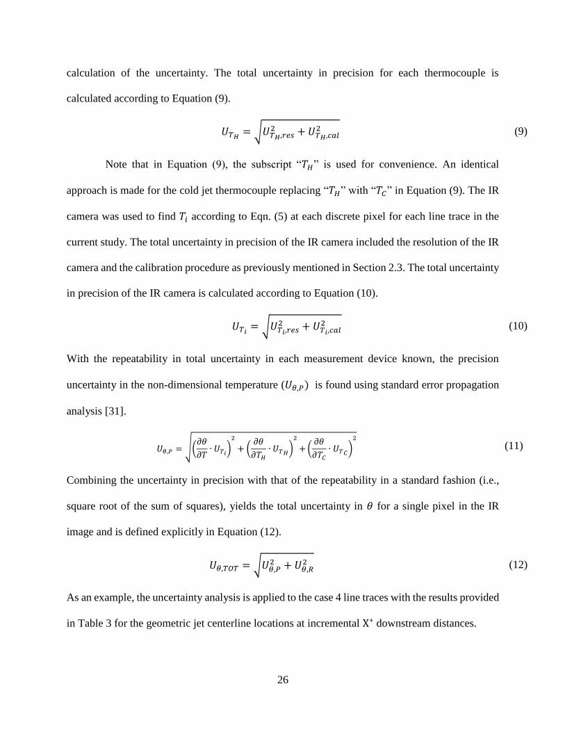
calculation of the uncertainty. The total uncertainty in precision for each thermocouple is

calculated according to Equation (9).

𝑈𝑇𝐻

= √𝑈𝑇𝐻,𝑟𝑒𝑠2 + 𝑈𝑇𝐻,𝑐𝑎𝑙

2 (9)

Note that in Equation (9), the subscript “𝑇𝐻” is used for convenience. An identical

approach is made for the cold jet thermocouple replacing “𝑇𝐻” with “𝑇𝐶” in Equation (9). The IR

camera was used to find 𝑇𝑖 according to Eqn. (5) at each discrete pixel for each line trace in the

current study. The total uncertainty in precision of the IR camera included the resolution of the IR

camera and the calibration procedure as previously mentioned in Section 2.3. The total uncertainty

in precision of the IR camera is calculated according to Equation (10).

𝑈𝑇𝑖

= √𝑈𝑇𝑖,𝑟𝑒𝑠2 + 𝑈𝑇𝑖,𝑐𝑎𝑙

2 (10)

With the repeatability in total uncertainty in each measurement device known, the precision

uncertainty in the non-dimensional temperature (𝑈𝜃,𝑃) is found using standard error propagation

analysis [31].

𝑈𝜃,𝑃 = √(𝜕𝜃

𝜕𝑇∙ 𝑈𝑇𝑖

)2

+ (𝜕𝜃

𝜕𝑇𝐻

∙ 𝑈𝑇𝐻)

2

+ (𝜕𝜃

𝜕𝑇𝐶

∙ 𝑈𝑇𝐶)

2

(11)

Combining the uncertainty in precision with that of the repeatability in a standard fashion (i.e.,

square root of the sum of squares), yields the total uncertainty in 𝜃 for a single pixel in the IR

image and is defined explicitly in Equation (12).

𝑈𝜃,𝑇𝑂𝑇 = √𝑈𝜃,𝑃

2 + 𝑈𝜃,𝑅2 (12)

As an example, the uncertainty analysis is applied to the case 4 line traces with the results provided

in Table 3 for the geometric jet centerline locations at incremental X∗ downstream distances.

27

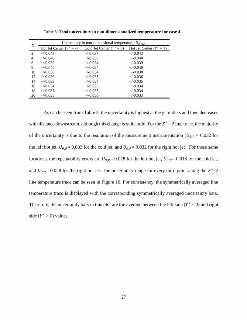
Table 3: Total uncertainty in non-dimensionalized temperature for case 4

𝑋∗

Uncertainty in non-dimensional temperature, 𝑈𝜃,𝑇𝑂𝑇

Hot Jet Center (𝑌∗ = -1) Cold Jet Center (𝑌∗ = 0) Hot Jet Center (𝑌∗ = 1)

2 +/-0.043 +/-0.037 +/-0.043

4 +/-0.040 +/-0.037 +/-0.040

6 +/-0.039 +/-0.034 +/-0.039

8 +/-0.040 +/-0.034 +/-0.040

10 +/-0.038 +/-0.034 +/-0.038

12 +/-0.036 +/-0.035 +/-0.036

14 +/-0.035 +/-0.034 +/-0.035

16 +/-0.034 +/-0.035 +/-0.034

18 +/-0.034 +/-0.035 +/-0.034

20 +/-0.033 +/-0.035 +/-0.033

As can be seen from Table 3, the uncertainty is highest at the jet outlets and then decreases

with distance downstream, although this change is quite mild. For the 𝑋∗ = 2 line trace, the majority

of the uncertainty is due to the resolution of the measurement instrumentation (𝑈𝜃,𝑃 = 0.032 for

the left hot jet, 𝑈𝜃,𝑃= 0.033 for the cold jet, and 𝑈𝜃,𝑃= 0.032 for the right hot jet). For these same

locations, the repeatability errors are 𝑈𝜃,𝑅= 0.028 for the left hot jet, 𝑈𝜃,𝑅= 0.018 for the cold jet,

and 𝑈𝜃,𝑅= 0.028 for the right hot jet. The uncertainty range for every third point along the 𝑋∗=2

line temperature trace can be seen in Figure 10. For consistency, the symmetrically averaged line

temperature trace is displayed with the corresponding symmetrically averaged uncertainty bars.

Therefore, the uncertainty bars in this plot are the average between the left side (𝑌∗ < 0) and right

side (𝑌∗ > 0) values.

28

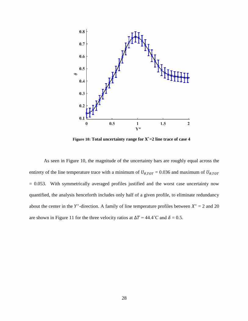
Figure 10: Total uncertainty range for 𝐗∗=2 line trace of case 4

As seen in Figure 10, the magnitude of the uncertainty bars are roughly equal across the

entirety of the line temperature trace with a minimum of 𝑈𝜃,𝑇𝑂𝑇 = 0.036 and maximum of 𝑈𝜃,𝑇𝑂𝑇

= 0.053. With symmetrically averaged profiles justified and the worst case uncertainty now

quantified, the analysis henceforth includes only half of a given profile, to eliminate redundancy

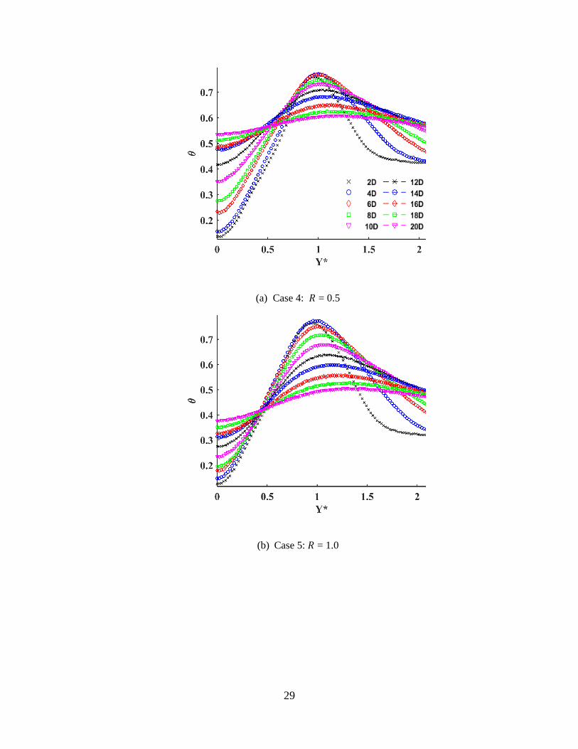
about the center in the 𝑌∗-direction. A family of line temperature profiles between 𝑋∗ = 2 and 20

are shown in Figure 11 for the three velocity ratios at ∆𝑇 = 44.4˚C and 𝛿 = 0.5.

29

(a) Case 4: 𝑅 = 0.5

(b) Case 5: 𝑅 = 1.0

30

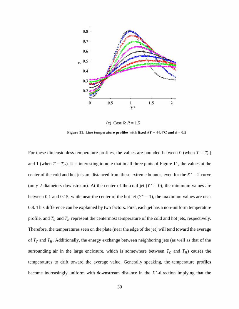
(c) Case 6: 𝑅 = 1.5

Figure 11: Line temperature profiles with fixed ∆T = 44.4˚C and δ = 0.5

For these dimensionless temperature profiles, the values are bounded between 0 (when 𝑇 = 𝑇𝐶)

and 1 (when 𝑇 = 𝑇𝐻). It is interesting to note that in all three plots of Figure 11, the values at the

center of the cold and hot jets are distanced from these extreme bounds, even for the 𝑋∗ = 2 curve

(only 2 diameters downstream). At the center of the cold jet (𝑌∗ = 0), the minimum values are

between 0.1 and 0.15, while near the center of the hot jet (𝑌∗ = 1), the maximum values are near

0.8. This difference can be explained by two factors. First, each jet has a non-uniform temperature

profile, and 𝑇𝐶 and 𝑇𝐻 represent the centermost temperature of the cold and hot jets, respectively.

Therefore, the temperatures seen on the plate (near the edge of the jet) will tend toward the average

of 𝑇𝐶 and 𝑇𝐻. Additionally, the energy exchange between neighboring jets (as well as that of the

surrounding air in the large enclosure, which is somewhere between 𝑇𝐶 and 𝑇𝐻) causes the

temperatures to drift toward the average value. Generally speaking, the temperature profiles

become increasingly uniform with downstream distance in the 𝑋∗-direction implying that the

31

temperature profile on the plate is becoming more evenly mixed. Although this is true for all three

plots in Figure 11, the impact of 𝑅 is easily seen when comparing the value of 𝜃 for the profile

closest to the fully mixed condition (𝑋∗= 20). In Figure 11(a), where 𝑅 = 0.5, the variation of

temperature at 𝑋∗ = 20 is bounded between 0.54 < 𝜃 < 0.61, while for 𝑅 = 1.0 (Figure 11(b)) these

bounds are between 0.38 and 0.51. When the cold jet velocity is highest (𝑅 = 1.5, Figure 11(c)),

these bounds naturally decrease further (0.31 < 𝜃 < 0.45). This behavior is qualitatively in line

with what one would expect for mixing of the two non-isothermal streams. If the settings listed in

Table 1 were applied to an analogous internal flow scenario, one could easily apply a mass energy

balance and predict the fully mixed temperatures. For the conditions employed in Figure 11, this

would suggest fully mixed dimensionless temperatures of 0.66, 0.52, and 0.42 for Figure 11(a),

(b), and (c), respectively. This implies that the upper limits of the 𝑋∗ = 20 non-dimensional

temperature profiles for each of the cases in Figure 11 are in good agreement with the theoretical

fully mixed temperatures from a mass energy balance perspective.

A conservative approach to defining a “uniformly mixed” profile would be the expectation

that sufficiently far downstream, and with no outside influence, the temperature profile will

become horizontal, such that for that profile, 𝜃 is a constant value such as those values proposed

by the mass energy balance analysis above. Interestingly, for the 𝑋∗ = 20 line trace, the average

value of 𝜃 (�̅�) and the maximum difference in values of 𝜃 across the line trace are �̅� = 0.58, 0.46,

0.40 and ∆𝜃𝑋∗=20 = 0.07, 0.13, 0.14 for Figure 11(a), (b), and (c), respectively. This implies that

with decreasing velocity ratios, 𝑅, the average non-dimensional temperature, �̅�, far downstream

increases yet the range in horizontal values of 𝜃 decreases. While a formal definition of the

“amount” of thermal mixing taking place on the plate surface is debatable, it is clear that the

32

decreasing values of velocity ratio promote uniformity in horizontal surface temperatures for the

test cases of Figure 11.

The 𝑅 = 0.5 condition as seen in Figure 11(a) displays the dominance of the hot jets on the

surface of the plate and the influence on the thermal mixing with increasing downstream distance.

The “washing out” of the cold jet previously alluded to in Section 3.1 is here quantitatively

evaluated as the aggressive shift in the non-dimensional surface temperature along 𝑌∗ = 0 (the cold

jet geometric center) with increasing downstream distance. At 𝑋∗ = 2 the cold jet centerline non-

dimensional temperature is 𝜃 = 0.14 and at 𝑋∗ = 20, is 𝜃 = 0.54, accounting for an increase of ∆𝜃

= 0.40. This shift in surface temperature across the 2 < 𝑋∗ < 20 region of the plate is much larger

when compared to the 𝑅 = 1.0 and 𝑅 = 1.5 conditions in Figure 11(b) and (c) which have shifts of

∆𝜃 = 0.25 and ∆𝜃 = 0.18, respectively. The same aggressive shift in surface temperature can be

seen around the hot jet center line 𝑌∗ = 1, for the 𝑅 = 1.5 condition of Figure 11(c) in which the

non-dimensional temperature at 𝑋∗ = 2 is 𝜃 = 0.80 and at 𝑋∗ = 20 is 𝜃 = 0.45, accounting for a of

∆𝜃 = -0.35. The shift in surface temperature around 𝑌∗ = 1, is significantly larger than those of 𝑅

= 0.5 in Figure 11(a) and 𝑅 = 1.0 in Figure 11(b), of which were 𝜃 = -0.15 and 𝜃 = -0.26,

respectively. While the downstream shift in surface temperature across the hot jet center line in

the 𝑅 = 1.5 condition is significant, it is not nearly as severe as that of the shift across the cold jet

centerline in the 𝑅 = 0.5 condition. This is attributed to the increased turbulence provided by the

𝑅 = 0.5 condition in case 4, in which all three jets operate at their maximum velocities relative to

all of the proposed test cases (as seen in Table 1). Recall that the cold jet velocity is fixed for all

of the proposed test cases, and therefore, the 𝑅 = 1.5 condition has the cold jet operating at a similar

Reynolds number as all other cases, with the hot jets flowing at two-thirds the flow rate of the

33

center cold jet, implying that the hot jets operate at much lower Reynolds numbers compared to

case 4.

More recent numerical work [8] involving a similar parallel triple slot jet configuration

with all isovelocity cases has suggested that with increasing Reynolds number, the mixing of hot

and cold fluid is delayed and the area of the convective mixing region is increased. A more

important fundamental understanding of the effect of the Reynolds number of the jets on the

induced convective mixing involves the present comparison of the non-isovelocity cases to an

isovelocity case at a fixed temperature difference. From the current analysis it is clear that the 𝑅=

0.5 condition, which includes the largest Reynolds numbers out of the three velocity ratios, reaches

a more uniform temperature across the 𝑌∗ direction of the plate further upstream than that of the

𝑅 = 1.0 or 𝑅 = 1.5 cases. The same behavior is seen in more detail by comparing the three plots

of Figure 11 with increasing downstream distance, the line traces of the temperature data for the

𝑅 = 0.5 case reach a horizontal value more rapidly than either of the other velocity cases.

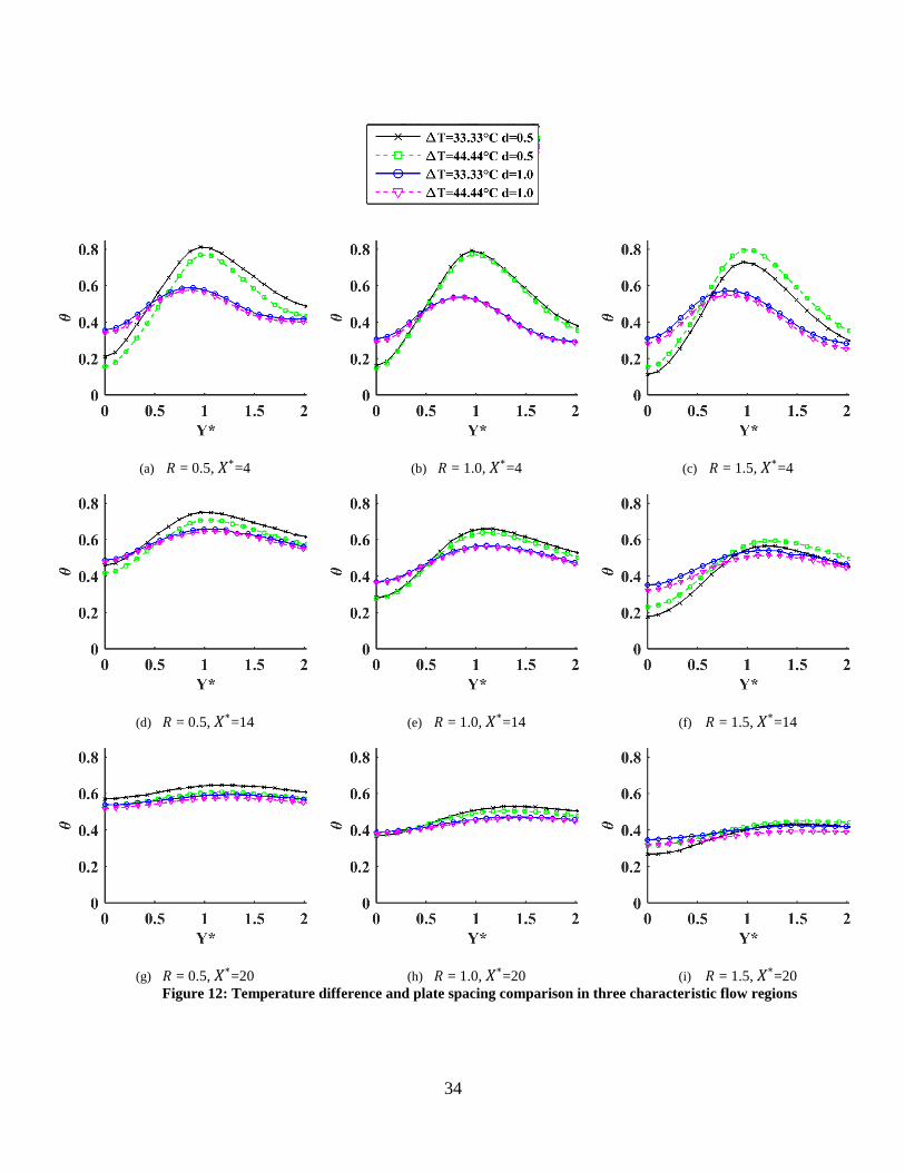
With the effect of the velocity ratio on the downstream temperature behavior understood,

further comparisons are made to quantify the effect of temperature difference between the jets

(∆𝑇) and the plate spacing (𝛿). This comparison is made by holding R constant, with results

presented in Figure 12. Each plot in this figure is at a fixed R and X*. The four curves represent

line traces similar to those in Figure 11, but now consider each unique ∆𝑇 and 𝛿 combination.

Three different 𝑋∗ downstream distances are analyzed, corresponding to the three regions of flow:

the entrance region (𝑋∗ = 4), the convective mixing region (𝑋∗ = 14), and the post-mixing region

(𝑋∗ = 20), as found in the top, middle, and bottom rows, respectively, of Figure 12.

34

(a) 𝑅 = 0.5, 𝑋∗=4

(b) 𝑅 = 1.0, 𝑋∗=4

(c) 𝑅 = 1.5, 𝑋∗=4

(d) 𝑅 = 0.5, 𝑋∗=14

(e) 𝑅 = 1.0, 𝑋∗=14

(f) 𝑅 = 1.5, 𝑋∗=14

(g) 𝑅 = 0.5, 𝑋∗=20

(h) 𝑅 = 1.0, 𝑋∗=20

(i) 𝑅 = 1.5, 𝑋∗=20

Figure 12: Temperature difference and plate spacing comparison in three characteristic flow regions

35

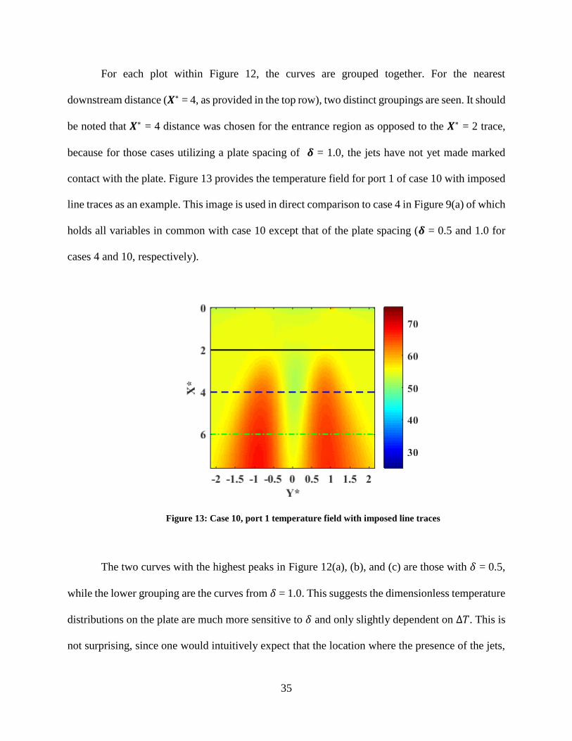
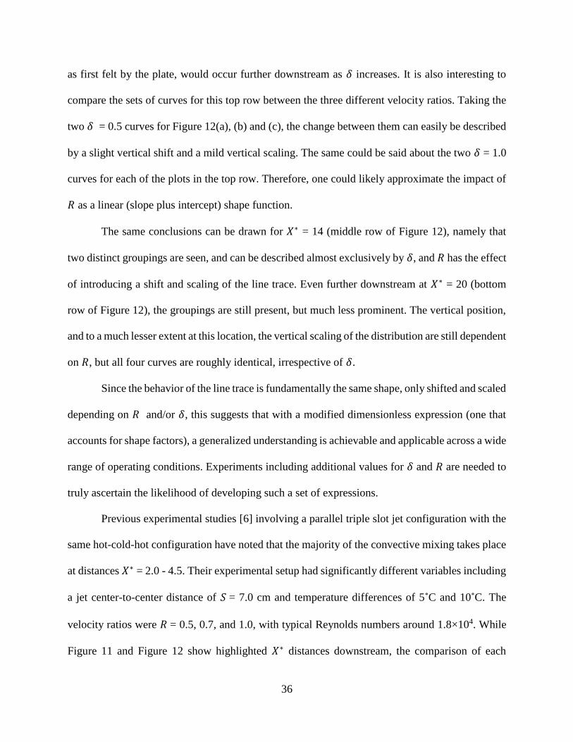
For each plot within Figure 12, the curves are grouped together. For the nearest

downstream distance (𝑿∗ = 4, as provided in the top row), two distinct groupings are seen. It should

be noted that 𝑿∗ = 4 distance was chosen for the entrance region as opposed to the 𝑿∗ = 2 trace,

because for those cases utilizing a plate spacing of 𝜹 = 1.0, the jets have not yet made marked

contact with the plate. Figure 13 provides the temperature field for port 1 of case 10 with imposed

line traces as an example. This image is used in direct comparison to case 4 in Figure 9(a) of which

holds all variables in common with case 10 except that of the plate spacing (𝜹 = 0.5 and 1.0 for

cases 4 and 10, respectively).

Figure 13: Case 10, port 1 temperature field with imposed line traces

The two curves with the highest peaks in Figure 12(a), (b), and (c) are those with 𝛿 = 0.5,

while the lower grouping are the curves from 𝛿 = 1.0. This suggests the dimensionless temperature

distributions on the plate are much more sensitive to 𝛿 and only slightly dependent on ∆𝑇. This is

not surprising, since one would intuitively expect that the location where the presence of the jets,

36

as first felt by the plate, would occur further downstream as 𝛿 increases. It is also interesting to

compare the sets of curves for this top row between the three different velocity ratios. Taking the

two 𝛿 = 0.5 curves for Figure 12(a), (b) and (c), the change between them can easily be described

by a slight vertical shift and a mild vertical scaling. The same could be said about the two 𝛿 = 1.0

curves for each of the plots in the top row. Therefore, one could likely approximate the impact of

𝑅 as a linear (slope plus intercept) shape function.

The same conclusions can be drawn for 𝑋∗ = 14 (middle row of Figure 12), namely that

two distinct groupings are seen, and can be described almost exclusively by 𝛿, and 𝑅 has the effect

of introducing a shift and scaling of the line trace. Even further downstream at 𝑋∗ = 20 (bottom

row of Figure 12), the groupings are still present, but much less prominent. The vertical position,

and to a much lesser extent at this location, the vertical scaling of the distribution are still dependent

on 𝑅, but all four curves are roughly identical, irrespective of 𝛿.

Since the behavior of the line trace is fundamentally the same shape, only shifted and scaled

depending on 𝑅 and/or 𝛿, this suggests that with a modified dimensionless expression (one that

accounts for shape factors), a generalized understanding is achievable and applicable across a wide

range of operating conditions. Experiments including additional values for 𝛿 and 𝑅 are needed to

truly ascertain the likelihood of developing such a set of expressions.

Previous experimental studies [6] involving a parallel triple slot jet configuration with the

same hot-cold-hot configuration have noted that the majority of the convective mixing takes place

at distances 𝑋∗ = 2.0 - 4.5. Their experimental setup had significantly different variables including

a jet center-to-center distance of 𝑆 = 7.0 cm and temperature differences of 5˚C and 10˚C. The

velocity ratios were 𝑅 = 0.5, 0.7, and 1.0, with typical Reynolds numbers around 1.8×104. While

Figure 11 and Figure 12 show highlighted 𝑋∗ distances downstream, the comparison of each

37

incremental 𝑋∗ distance downstream done in the current study suggests that for the parallel round

triple round jet configuration, the dominant convective mixing region occurs in the 8 < 𝑋∗ < 16

region. Interestingly, with a jet spacing approximately half as large as that used in the slot jet study

and the differences in the jet outlet geometry considered, the convective mixing region is on the

order of three times as large for the round jet observations as that of the slot jet study.

3.3 LOCATIONS OF MAXIMUM TEMPERATURE

The data contained in Figure 11 is analyzed in terms of the maximum temperature location and its

variation as the flow travels downstream. This is provided in Figure 14, and is an indicator of the

degree to which the hot jet veers away from the cold central jet.

(a) ∆𝑇 = 33.33˚C, 𝛿 = 0.5

(b) ∆𝑇 = 33.33˚C, 𝛿 = 1.0

38

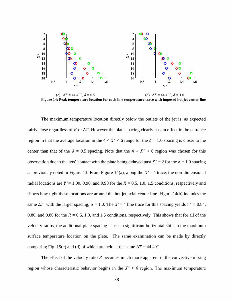
(c) ∆𝑇 = 44.4˚C, 𝛿 = 0.5

(d) ∆𝑇 = 44.4˚C, 𝛿 = 1.0

Figure 14: Peak temperature location for each line temperature trace with imposed hot jet center line

The maximum temperature location directly below the outlets of the jet is, as expected

fairly close regardless of 𝑅 or ∆𝑇. However the plate spacing clearly has an effect in the entrance

region in that the average location in the 4 < 𝑋∗ < 6 range for the 𝛿 = 1.0 spacing is closer to the

center than that of the 𝛿 = 0.5 spacing. Note that the 4 < 𝑋∗ < 6 region was chosen for this

observation due to the jets’ contact with the plate being delayed past 𝑋∗ = 2 for the 𝛿 = 1.0 spacing

as previously noted in Figure 13. From Figure 14(a), along the 𝑋∗= 4 trace, the non-dimensional

radial locations are 𝑌∗= 1.00, 0.96, and 0.98 for the 𝑅 = 0.5, 1.0, 1.5 conditions, respectively and

shows how tight these locations are around the hot jet axial center line. Figure 14(b) includes the

same ∆𝑇 with the larger spacing, 𝛿 = 1.0. The 𝑋∗= 4 line trace for this spacing yields 𝑌∗ = 0.84,

0.80, and 0.80 for the 𝑅 = 0.5, 1.0, and 1.5 conditions, respectively. This shows that for all of the

velocity ratios, the additional plate spacing causes a significant horizontal shift in the maximum

surface temperature location on the plate. The same examination can be made by directly

comparing Fig. 15(c) and (d) of which are held at the same ∆𝑇 = 44.4˚C.

The effect of the velocity ratio 𝑅 becomes much more apparent in the convective mixing

region whose characteristic behavior begins in the 𝑋∗ ≈ 8 region. The maximum temperature

39

location spreads more sporadically in the 𝑌∗ direction with increasing values of 𝑅, and this

behavior is consistent for each combination of ∆𝑇 and δ. For instance, in Figure 14(c) the location

of the maximum temperature from the chosen initial location 𝑋∗ = 4, to four times this distance

downstream, 𝑋∗ = 16, changes by a non-dimensional radial distance of ∆𝑌∗ = 0.13, 0.32, and 0.41

for the 𝑅 = 0.5, 1.0, and 1.5 conditions, respectively. From similar inspection of the other plots of

Figure 14, it is clear that the same conclusion can be drawn from each: with the velocity ratio 𝑅

being the main variable driving thermal mixing in the convective mixing region, increasing values

of 𝑅 allow the influence of the cold jet to push out the hot jets. This in turn dissipates the influence

of the hot jets on the plate, promoting thermal mixing of each hot jet separately with the cold jet,

as opposed to the behavior of the 𝑅 = 0.5 condition in which the opposite is true. By dissipating

the influence of the cold jet on the plate, the maximum temperature on the surface of the plate

should spread far less significantly, as is apparent with the much smaller ∆𝑌∗ in the region 4 < 𝑋∗

< 16.

As far as 𝑋∗ = 10 downstream, the relative maximum temperature locations for a given

case are fairly predictable, implying that the data could be explained through correlations.

However, past the 𝑋∗ = 10 mark, the locations for a given case become increasingly more sporadic.

This observation provides support for the lower limit (𝑋∗ < 16) of the downstream range in the

∆𝑌∗ comparison above. The sporadic nature of the maximum temperature locations is explained

in part by the convective mixing phenomena itself, however the increasing fluctuations further

downstream are explained by the influence of the total mass entrained by the jets with increasing

downstream distance. The increasing influence of the total mass and the significant decrease in

momentum far downstream implies that the maximum temperature on the plate surface is subject

to some fluctuation, as is characteristic of the post mixing region, and a trend line in this region is

40

no longer justified. This conclusion is in good standing with the observations made earlier in

Section 3.2 regarding the uniform mixing far downstream in Figure 11 and justifies the transition

area from the convective mixing region to the post mixing region as 𝑋∗ ≈ 16.

41

4.0 CONCLUSIONS

An experimental study of the interaction of three non-isothermal parallel round jets is conducted

in a planar hot-cold-hot configuration. The jets are operated within the turbulent regime with a jet

Reynolds number between 5.5 × 103 and 1.8 × 104 at three distinct cold to hot jet velocity ratios

(R = 0.50, 1.00, 1.51). A flat polycarbonate plate is mounted parallel to the axial direction of the

jets, and is offset in two different spacings: one half and one full jet diameter from the axial

direction of the jets (𝛿 = 0.5, 1.0). The downstream thermal mixing of the jets are studied with

temperature differences of ∆𝑇 = 33.33˚C and 44.4 ˚C between the cold and hot jets. Steady-state

results are captured via infrared thermography and indicate the thermal loading on the plate. The

velocities of the individual jets are compared via the extreme velocity ratio cases 𝑅 = 0.50 and

1.51 to that of the isovelocity case. The induced thermal line signatures on the plate surface suggest

the most aggressive shifts in temperature occur in the area characteristic of the convective mixing

region, defined here as the range 8 < 𝑋∗< 16.

Qualitative thermal fields are analyzed with horizontal line traces of the plate surface

temperature at downstream distances from the outlets of the jets in the range 2 < 𝑋∗ < 20. With a

constant cold jet velocity for all cases, increasing hot jet velocities induce more turbulent mixing

particularly in the convective mixing region promoting thermal mixing further upstream than that

of the lower hot jet velocity cases. Interestingly, with increasing hot jet velocities, it is also found

that while the average non-dimensional temperature far downstream (𝑋∗ = 20) increases, the range

42

in values across this thermal signature decreases. Far downstream mixing behavior is in good

quantitative agreement with the fully mixed temperature expected from a mass energy balance

approach.

By holding the velocity ratio constant, thermal signatures are also found to be highly dependent

on the plate spacing and that the temperature differences considered in this study provided little

influence. Results suggest the highest temperature differences on the surface of the plate occur in

the plane common to the three jet axes. Additionally, for a give value of 𝑅, the thermal traces reach

nearly identical values far downstream in the post mixing region, here defined as 𝑋∗ > 16

regardless of plate spacing 𝛿 or temperature difference ∆𝑇.

The peak temperature location on the surface of the plate at each downstream temperature trace

is also of considerable interest in describing the overall shift in the transfer of heat across the

surface of the plate. The maximum temperature location in the entrance region (2 < 𝑋∗ < 8) is

almost exclusively dependent on plate spacing 𝛿 with little influence from the velocity ratio 𝑅 or

temperature difference ∆𝑇. In the 2 < 𝑋∗< 6 range, the 𝛿 = 1.0 spacing provides maximum

temperatures closer to the axial center of the cold jet (𝑌∗ = 0) than that of the 𝛿 = 0.5 spacing. The

effect of 𝑅 becomes much more apparent in the convective mixing region where the maximum

temperatures spread further in the 𝑌∗-direction with increasing 𝑅, and this behavior is found to be

consistent for each combination of ∆𝑇 and 𝛿. The maximum temperature locations for a given case

are found to be predictable as far as 𝑋∗ = 10 downstream, but become increasingly more sporadic

past this length. This is attributed to the increase in the total mass entrained by the jets and the

decreasing influence of the momentum with increasing downstream distance.

This research represents preliminary predictions of the thermal loading in the VHTR lower

plenum and provides validation data for fundamental and applied thermal mixing simulations.

43

With future verified computational analysis, the determination of the thermal loading as a function

of the jet Reynolds numbers, the temperature difference between the jets, and the plate position

can be found. These studies provide for useful insight in preventing thermal striping in the internal

structural walls of the VHTR lower plenum and can be utilized in future work in material analysis

of structural integrity in the VHTR core.

44

BIBLIOGRAPHY

[1] P.E. MacDonald, P.D. Bayless, H.D. Gougar, R.L. Moore, A.M. Ougouag, R.L. Sant, J.W.

Sterbentz, W.K. Terry, The Next Generation Nuclear Plant – Insights Gained from the INEEL

Point Design Studies, in: Proceedings of the 2004 International Congress on Advances in Nuclear

Power Plants (ICAPP '04), Pittsburgh, PA, USA, 2004.

[2] S.B. Rodriguez, M.S. El-Genk, Numerical investigation of potential elimination of ‘hot

streaking’ and stratification in the VHTR lower plenum using helicoid inserts, Nuclear

Engineering and Design, 240(5) (2010) 995-1004.

[3] C. Betts, C. Boorman, N. Sheriff, Thermal Striping in Liquid Cooled Fast Breeder Reactors,

Thermal Hydraulics of Nuclear Reactors, (1983) 1292-1301.

[4] A.M. Clayton, Thermal Shock in Nuclear Reactors, Progress in Nuclear Energy, 12(1) (1983)

57-83.

[5] G.J. Lloyd, D.S. Wood, Fatigue Crack Initiation And Propogation as a Consequence of

Thermal Striping, International Journal of Pressure Vessels and Piping, 8 (1980) 255-272.

[6] A. Tokuhiro, N. Kimura, An experimental investigation on thermal striping mixing phenomena

of a vertical non-buoyant jet with two adjacent buoyant jets as measured by ultrasound Doppler

velocimetry, Nuclear Engineering and Design, 188 (1999) 49-73.

[7] R.D. Blevins, Applied Fluid Dynamics Handbook, Van Nostrand Reinhold Co., New York,

1984.

[8] Q. Cao, D. Lu, J. Lv, Numerical investigation on temperature fluctuation of the parallel triple-

jet, Nuclear Engineering and Design, 249 (2012) 82-89.

[9] N. Kimura, M. Nishimura, H. Kamide, Study on Convective Mixing for Thermal Striping

Phenomena, Japan Society of Mechanical Engineers International Journal, 45(3) (2002) 592-599.

[10] M. Nishimura, A. Tokuhiro, N. Kimura, H. Kamide, Numerical study on mixing of oscillating

quasi-planar jets with low Reynolds number turbulent stress and heat flux equation models,

Nuclear Engineering and Design, 202 (2000) 77-95.

45

[11] N. Kimura, H. Miyakoshi, H. Kamide, Experimental investigation on transfer characteristics

of temperature fluctuation from liquid sodium to wall in parallel triple-jet, International Journal of

Heat and Mass Transfer, 50(9-10) (2007) 2024-2036.

[12] I.S. Jones, M.W.J. Lewis, An Impulse Response Model for the Prediction of Thermal Striping

Damage, Engineering Fracture Mechanics, 55(5) (1996) 795-812.

[13] N. Kasahara, H. Takasho, A. Yacumpai, Structural response function approach for evaluation

of thermal striping phenomena, Nuclear Engineering and Design, 212 (2002) 281-292.

[14] R.E. Spall, E.A. Anderson, J. Allen, Momentum Flux in Plane, Parallel Jets, Journal of Fluids

Engineering, 126(4) (2004) 665.

[15] D. Tenchine, S. Vandroux, V. Barthel, O. Cioni, Experimental and numerical studies on

mixing jets for sodium cooled fast reactors, Nuclear Engineering and Design, 263 (2013) 263-272.

[16] S.-K. Choi, S.-O. Kim, Evaluation of Turbulence Models for Thermal Striping in a Triple Jet,

Journal of Pressure Vessel Technology, 129 (2007) 583-592.

[17] S.B. Pope, An Explanation of the Turbulent Round-Jet/Plane-Jet Anomaly, American Institute

of Aeronautics and Astronautics, 16(3) (1978) 279-281.

[18] H. Schlichting, Boundary-Layer Theory, 7 ed., McGraw-Hill Book Company, 1979.

[19] J. Boulanger, L. Vervisch, J. Reveillon, S. Ghosal, Effects of heat release in laminar diffusion

flames lifted on round jets, Combustion and Flame, 134(4) (2003) 355-368.

[20] S.D. Hwang, H.H. Cho, Effects of Acoustic Excitation Positions on Heat Transfer and Flow

in Axisymmetric Impinging Jet: Main Jet Excitation and Shear Layer Excitation, International

Journal of Heat and Fluid Flow, 24(2) (2003) 199-209.

[21] A. Pavlova, M. Amitay, Electronic Cooling Using Synthetic Jet Impingement, Journal of Heat

Transfer, 128(9) (2006) 897.

[22] N. Amini, Y.A. Hassan, Measurements of jet flows impinging into a channel containing a rod

bundle using dynamic PIV, International Journal of Heat and Mass Transfer, 52(23-24) (2009)

5479-5495.

[23] K.G. Condie, G.E. McCreery, H.M. McIllroy, D.M. McEligot, Development of an

Experiment for Measuring Flow Phenomena Occuring in a Lower Plenum for VHTR CFD

Assessment, in: D.o.E.O.o.N. Energy (Ed.), Idaho National Laboratory, Idaho Falls, Idaho 83415,

2005.

[24] H.M. McIlroy, D.M. McEligot, R.R. Schultz, D. Christensen, R.J. Pink, R.C. Johnson, PIV

Experiments to Measure Flow Phenomena in a Scaled Model of a VHTR Lower Plenum, in:

D.o.E.O.o.N. Energy (Ed.), Idaho National Laboratory, Idaho Falls, ID 83415, 2006.

46

[25] H. Haque, W. Feltes, G. Brinkmann, Thermal response of a modular high temperature reactor

during passive cooldown under pressurized and depressurized conditions, Nuclear Engineering

and Design, 236(5-6) (2006) 475-484.

[26] K.L. McVay, J.-H. Park, S. Lee, Y.A. Hassan, N.K. Anand, Preliminary tests of particle image

velocimetry for the upper plenum of a scaled model of a very high temperature gas cooled reactor,

Progress in Nuclear Energy, 83 (2015) 305-317.

[27] NASA jet Propulsion Laboratory Web Site in, 1997, pp.

http://masterweb.jpl.nasa.gov/reference/images/paints/Best%204%220paints%220MWIR.gif.

[28] D.T. Landfried, Experimental and Computational Studies of Thermal Mixing in Next

Generation Nuclear Reactors, Doctorate of Philosophy, University of Pittsburgh, Pittsburgh, PA,

2015.

[29] G.E. McCreery, K.G. Condie, Experimental Modeling of VHTR Plenum Flows During

Normal Operation and Pressurized Conduction Cooldown, in: D.o.E.O.o.N. Energy (Ed.), Idaho

National Laboratory, Idaho Falls, Idaho 83415, 2006.

[30] S. Moriya, I. Ohshima, Hydraulic Similarity in the Temperature Fluctuation Phenomena of

Non-Isothermal Coaxial Jets, Nuclear Engineering and Design, 120 (1990) 385-393.

[31] R.S. Figliola, D.E. Beasley, Theory and Design for Mechanical Measurements, John Wiley

& Sons, Inc., 2011.