Experimental System for Predicting Shelf-Slope Optics (ESPreSSO):

Assimilating ocean color data using an iterative ensemble smoother:

skill assessment for a suite of dynamical and error models

Dennis McGillicuddyKeston Smith

Ocean color assimilation as a solution to the cloudiness problem

State estimation (compositing)Process studies

SW06 data – Gawarkiewicz et al.

Methodology

cyxR

yxScDcvt

c

),(

),(

0

Forward model (2-D):

c: surface layer (20m) chlorophyll concentrationv: velocity provided by hydrodynamic modelD: diffusivity, 10 m s-2

S(x,y), R(x,y): unknown source/sink terms

Data (d): trueHcd

H: linear measurement operatorη: measurement error

Approach: Utilize an ensemble (N=400) of Monte Carlo simulations to estimate initial conditions c(t0) and source/sink terms S(x,y), R(x,y)

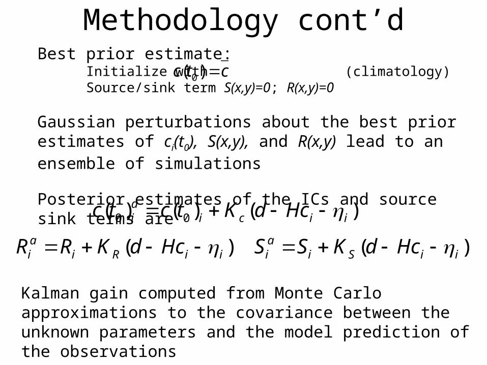
Methodology cont’dBest prior estimate:

Initialize with (climatology)Source/sink term S(x,y)=0; R(x,y)=0

Posterior estimates of the ICs and source sink terms are

ctc )( 0

)()()( 00 iiciai HcdKtctc

)( iiRiai HcdKRR )( iiSi

ai HcdKSS

Gaussian perturbations about the best prior estimates of ci(t0), S(x,y), and R(x,y) lead to an ensemble of simulations

Kalman gain computed from Monte Carlo approximations to the covariance between the unknown parameters and the model prediction of the observations

Use of an explicit biological model

nppnDnvt

n

pnppDpvt

p

Phytoplankton:

Nutrients:

Satellite ocean color data samples the phytoplankton field:

Hpd

Model domains

Shelf-scale ROMS(9km resolution)He and Chen, submitted

Assimilationsubdomain

Region ofinterest

Mean of the prior initial conditions: MODIS climatology for August

Chlorophyll a – mg m-3

Velocity Field 9km ROMS time-mean for Jul 25-Sept 9

Results

Prior

RHS=0

RHS=S(x,y)

RHS=R(x,y)c

N-P model

Satellitedata

Ernesto

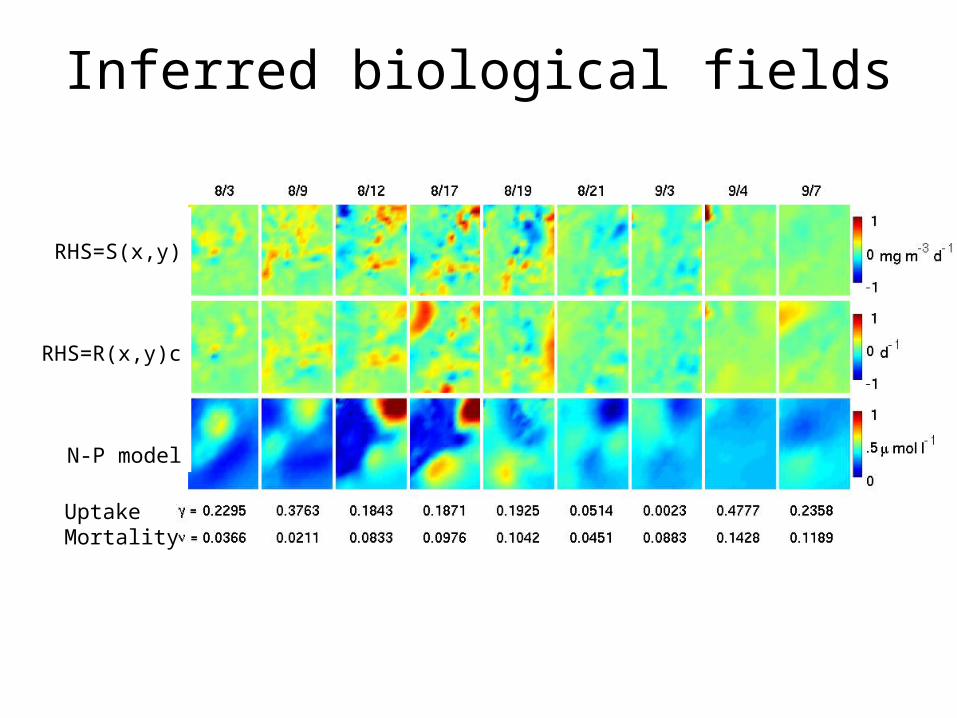
Inferred biological fields

RHS=S(x,y)

RHS=R(x,y)c

N-P model

UptakeMortality

Skill assessment: sensitivity to observational error

Observational error standard deviation

RM

S m

isfit

to

unas

sim

ilate

d da

tapassive

posteriorpassive

passiveprior

passive

dcH

dcHskill

ADR 43%ADS 36%NP 32%AD 18%

Comparisons with Gawarkiewicz in situ data

Comparisons with Gawarkiewicz in situ data

Year Day

Cor

rela

tion

Model vs. in situ

Model vs. satellite Satellite vs. in situ

Ernesto

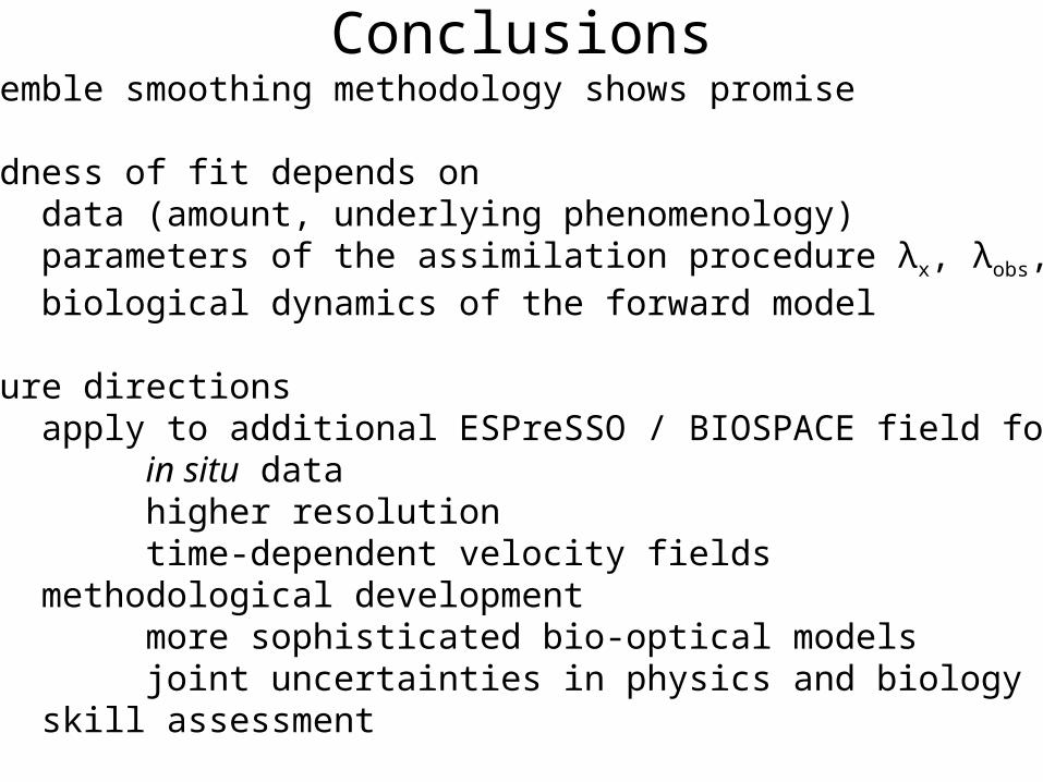
ConclusionsEnsemble smoothing methodology shows promise

Goodness of fit depends ondata (amount, underlying phenomenology)parameters of the assimilation procedure λx, λobs, σobs

biological dynamics of the forward model

Future directionsapply to additional ESPreSSO / BIOSPACE field foci

in situ datahigher resolutiontime-dependent velocity fields

methodological developmentmore sophisticated bio-optical modelsjoint uncertainties in physics and biology

skill assessment

Extras

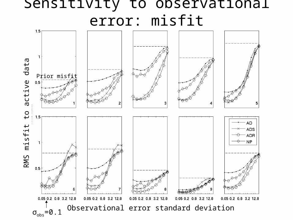
Sensitivity to observational error: misfit

Observational error standard deviation

RM

S m

isfit

to

activ

e da

ta Prior misfit

σobs=0.1

Necessity of an iterative approach

Methodology (3)Posterior estimates of the ICs and source sink terms are

)()()( 00 iiciai HcdKtctc

1)( WHPHHPK TTcc

obs

jiobsji

xxW

||exp2

,

Kalman gain computed from observational error covariance W and the ensemble covariances P, Pc, and PR

with

)( iiRiai HcdKRR

1)( WHPHHPK TTRR

km 25

m mg 1 32

obs

obs

)( iiSiai HcdKSS

1)( WHPHHPK TTSS

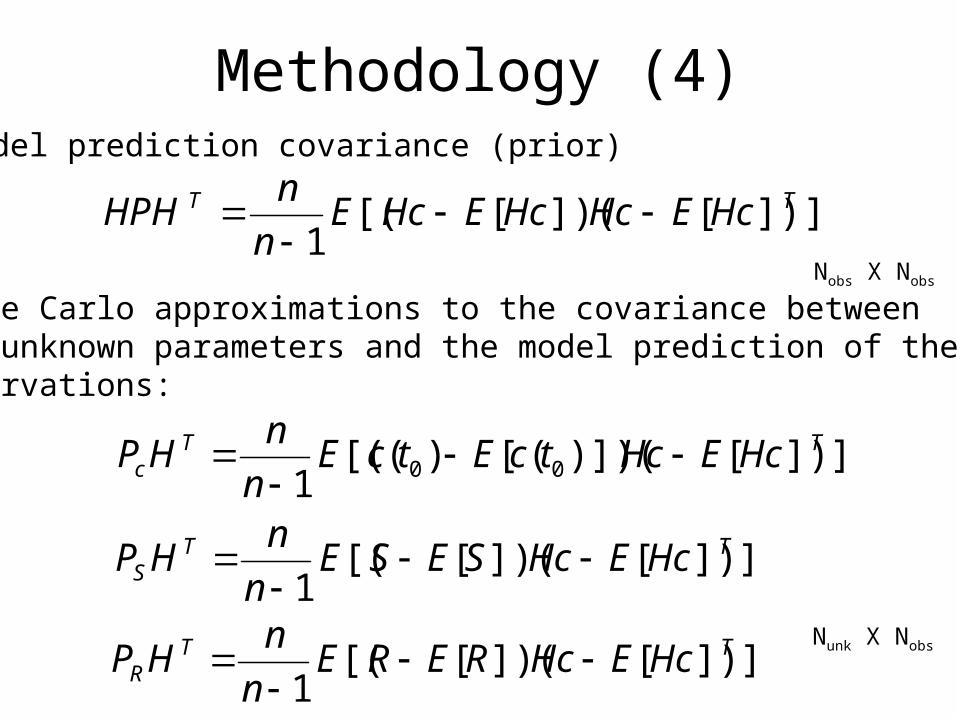
Methodology (4)Model prediction covariance (prior)

Monte Carlo approximations to the covariance betweenthe unknown parameters and the model prediction of theobservations:

]])[)])(([)([(1 00

TTc HcEHctcEtcE

n

nHP

]])[])([[(1

TTR HcEHcRERE

n

nHP

]])[])([[(1

TT HcEHcHcEHcEn

nHPH

Nobs X Nobs

Nunk X Nobs

]])[])([[(1

TTS HcEHcSESE

n

nHP

Methodology cont’dBest prior estimate:

Initialize with (climatology)Source/sink term S(x,y)=0; R(x,y)=0

Gaussian perturbations about the best prior estimates of ci(t0), S(x,y), and R(x,y) lead to an ensemble of simulations

Posterior estimates of the ICs and source sink terms are

ctc )( 0

)()()( 00 iiciai HcdKtctc

)( iiRiai HcdKRR )( iiSi

ai HcdKSS

Kalman gain computed from Monte Carlo approximations to the covariance between the unknown parameters and the model prediction of the observations