Embed Size (px)
Citation preview
Experimental Verification of Common-Mode Current Generation in Home Electrical Wiring in the Poweline Communications Band
A. Rubinstein1 , A. Vukicevic2, M.Rubinstein1, F. Rachidi2
1 University of Applied Sciences of Western Switzerland, Yverdon, Switzerland.
[email protected], [email protected]
2Swiss Federal Institute of Technology (EPFL), EMC Group, Lausanne, Switzerland. [email protected], [email protected]
Abstract
This paper presents a test of the relation between the common mode current in the cabling inside a home and the common and differential mode signals injected into any other part of the cabling in the house. The results are in satisfactory agreement with the hypothesis that the common mode current at any point inside the house can be calculated by computing the linear combination of the effects of the two input modes.
1. Introduction Powerline communications (PLC) or Broadband Powerline (BPL) is a technology for data transmission in the last mile and in-home. Since it uses existing electrical cabling as a transmission medium, and since such cabling is present in most households, PLC exhibits great a priori potential and in may become a competitor to other technologies such as DSL or wireless. In addition, whereas the number of telephone outlets per household tends to be low in many countries (one or two per home), there is usually at least one power outlet in every room. On the other hand, EMC issues, achievable throughputs and proper marketing are likely to play a decisive role in the commercial success the technology. Emissions from PLC transmissions inside the home are due essentially to common mode currents in the intrinsically asymmetrical electrical cabling. The common mode appears to be related to asymmetries in the home wiring, such as unequal distances of conductors to the ground, open switches, etc [1]. In this paper, we test a simple formula that assumes that the common mode any place in the home can be calculated by adding the contributions to it due to the differential mode and the common mode injected elsewhere in the house. This simple approach can be extended to calculate the common mode by superposition of all of the differential and common mode sources around the house, although the required transfer functions, which we obtained experimentally in the present paper, would need to be obtainable through theoretical modeling for the technique to become widely applicable in practice.
2. Experimental Set-Up
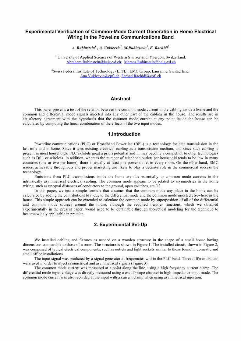
We installed cabling and fixtures as needed on a wooden structure in the shape of a small house having dimensions comparable to those of a room. The structure is shown in Figure 1. The installed circuit, shown in Figure 2, was composed of typical electrical components, such as outlets and light sockets similar to those found in domestic and small office installations. The input signal was produced by a signal generator at frequencies within the PLC band. Three different baluns were used in order to inject symmetrical and asymmetrical signals (Figure 3). The common mode current was measured at a point along the line, using a high frequency current clamp. The differential mode input voltage was directly measured using a oscilloscope channel in high-impedance input mode. The common mode current was also recorded at the input with a current clamp when using asymmetrical injection.
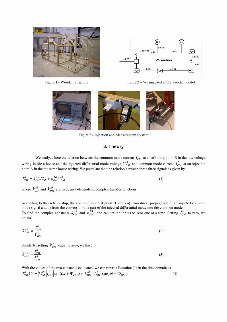
Figure 1 - Wooden Structure
Figure 2 – Wiring used in the wooden model
Figure 3 - Injection and Measurement System
3. Theory
We analyze here the relation between the common mode current
!
ICM
B at an arbitrary point B in the low voltage wiring inside a house and the injected differential mode voltage
!
VDM
A and common mode current
!
ICM
A at an injection point A in the the same house wiring. We postulate that the relation between these three signals is given by
!
ICM
B= k
CM
ABICM
A+ k
DM
ABVDM
A (1) where
!
kCM
AB and
!
kDM
AB are frequency-dependent, complex transfer functions. According to this relationship, the common mode at point B stems a) from direct propagation of an injected common mode signal and b) from the conversion of a part of the injected differential mode into the common mode. To find the complex constants
!
kCM
AB and
!
kDM
AB , one can set the inputs to zero one at a time. Setting
!
ICM
A to zero, we obtain
!
kDM
AB=ICM
B
VDM
A (2)
Similarly, setting
!
VDM
A equal to zero, we have
!
kCM
AB=ICM
B
ICM
A (3)
With the values of the two constants evaluated, we can rewrite Equation (1) in the time domain as
!
ICM
B(t) = k
CM
ABICM
Asin("t +#
CM) + k
DM
ABVDM
Asin("t +#
DM) (4)
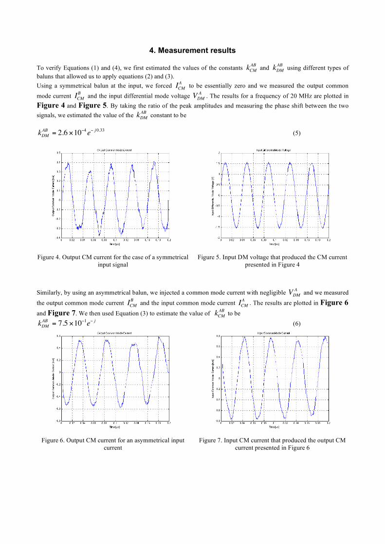
4. Measurement results To verify Equations (1) and (4), we first estimated the values of the constants
!
kCM
AB and
!
kDM
AB using different types of baluns that allowed us to apply equations (2) and (3). Using a symmetrical balun at the input, we forced
!
ICM
A to be essentially zero and we measured the output common mode current
!
ICM
B and the input differential mode voltage
!
VDM
A . The results for a frequency of 20 MHz are plotted in Figure 4 and Figure 5. By taking the ratio of the peak amplitudes and measuring the phase shift between the two signals, we estimated the value of the
!
kDM
AB constant to be
!
kDMAB
= 2.6 "10#4e# j 0.33 (5)
Figure 4. Output CM current for the case of a symmetrical
input signal
Figure 5. Input DM voltage that produced the CM current
presented in Figure 4
Similarly, by using an asymmetrical balun, we injected a common mode current with negligible
!
VDM
A and we measured the output common mode current
!
ICM
B and the input common mode current
!
ICM
A . The results are plotted in Figure 6 and Figure 7. We then used Equation (3) to estimate the value of
!
kCM
AB to be
!
kDMAB
= 7.5 "10#1e# j (6)
Figure 6. Output CM current for an asymmetrical input
current
Figure 7. Input CM current that produced the output CM
current presented in Figure 6
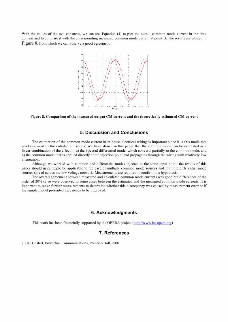
With the values of the two constants, we can use Equation (4) to plot the output common mode current in the time domain and to compare it with the corresponding measured common mode current at point B. The results are plotted in Figure 8, from which we can observe a good agreement.
Figure 8. Comparison of the measured output CM current and the theoretically estimated CM current
5. Discussion and Conclusions The estimation of the common mode current in in-house electrical wiring is important since it is this mode that
produces most of the radiated emissions. We have shown in this paper that the common mode can be estimated as a linear combination of the effect of a) the injected differential mode, which converts partially to the common mode, and b) the common mode that is applied directly at the injection point and propagates through the wiring with relatively low attenuation.
Although we worked with common and differential modes injected at the same input point, the results of this paper should in principle be applicable to the case of multiple common mode sources and multiple differential mode sources spread across the low voltage network. Measurements are required to confirm this hypothesis.
The overall agreement between measured and calculated common mode currents was good but differences of the order of 20% or so were observed in some cases between the estimated and the measured common mode currents. It is important to make further measurements to determine whether this discrepancy was caused by measurement error or if the simple model presented here needs to be improved.
6. Acknowledgments
This work has been financially supported by the OPERA project (http://www.ist-opera.org)
7. References [1] K. Dostert, Powerline Communications, Prentice-Hall, 2001.