Embed Size (px)
Citation preview

University of Arkansas, FayettevilleScholarWorks@UARK
Theses and Dissertations
12-2018
Experimentation and Modeling of the Effects ofAlong-Wind Dispersion on Cloud Characteristicsof Finite-Duration Contaminant Releases in theAtmosphereJessica M. MorrisUniversity of Arkansas, Fayetteville
Follow this and additional works at: https://scholarworks.uark.edu/etd
Part of the Process Control and Systems Commons
This Dissertation is brought to you for free and open access by ScholarWorks@UARK. It has been accepted for inclusion in Theses and Dissertations byan authorized administrator of ScholarWorks@UARK. For more information, please contact [email protected], [email protected].
Recommended CitationMorris, Jessica M., "Experimentation and Modeling of the Effects of Along-Wind Dispersion on Cloud Characteristics of Finite-Duration Contaminant Releases in the Atmosphere" (2018). Theses and Dissertations. 3088.https://scholarworks.uark.edu/etd/3088

Experimentation and Modeling of the Effects of Along-Wind Dispersion on Cloud
Characteristics of Finite-Duration Contaminant Releases in the Atmosphere
A dissertation submitted in partial fulfillment
of the requirements for the degree of
Doctor of Philosophy in Chemical Engineering
by
Jessica M. Morris
University of Minnesota
Bachelor of Science in Chemical Engineering, 2014
December 2018
University of Arkansas
This dissertation is approved for recommendation to the Graduate Council
_________________________________
Tom O. Spicer III, Ph.D., P.E.
Dissertation Director
_________________________________ _________________________________
Jerry Havens, Ph.D. Heather Walker, Ph.D.
Committee Member Committee Member
_________________________________ _________________________________
Larry Roe, Ph.D. David Ford, Ph.D.
Committee Member Committee Member

Abstract
Along-wind dispersion, or stretching of the cloud in the direction of the wind, plays an important
role in the concentration and modeling of contaminant releases in the atmosphere. Theoretical and
empirical derivations were compared for appropriate parameterization of along-wind dispersion.
Available field data were analyzed to evaluate and improve previous parameterizations of the
along-wind dispersion coefficient, 𝜎𝑥. An experimental test program was developed and executed
in an ultra-low speed wind tunnel at the Chemical Hazards Research Center to determine the
effects of the time distribution coefficient on true finite-duration releases from an original area
source. Multiple wind speeds, release durations, and downwind distances were investigated with
ensemble averages for improved quality of the cloud characteristics for each set of test conditions.
An overall relationship between the time of peak arrival (TOPa) and the time distribution
coefficient 𝜎𝑡 = 0.23 ∗ 𝑇𝑂𝑃𝑎 was demonstrated across all parameters. From this relationship, the
along-wind dispersion coefficient can be accurately predicted and scaled appropriately. Additional
relationships for the leading and trailing edges of the cloud are appropriately modeled.

©2018 by Jessica M. Morris
All Rights Reserved

Project Overview
Continued worldwide industrial development has brought the widespread use of industrial
chemicals, many of which are hazardous. Whether released accidentally or intentionally, air born
hazardous chemicals can affect large populations quickly as evidenced by several industrial
chemical accidents (e.g., Bhopal1, Flixborough2, Seveso3, etc.). Understanding and modeling
hazardous chemical releases are vital to protecting the public. The ability to predict the potential
impact of hazardous gas releases in the atmosphere is imperative to properly determine the
transport, storage, and use of such chemicals. In the case of an actual loss of containment,
understanding where air born chemicals can travel is important to determine the proper response
to an emergency.
Researchers have worked to assess these hazards through instantaneous, continuous, and time-
limiting experimental releases to develop computational models such as PHAST, HEGADAS, and
SLAB. Although instantaneous and continuous models are sufficient for many release scenarios,
many real-world problems involve finite-duration releases. Advanced computational fluid
dynamics (CFD) models can theoretically handle these complexities, but these models still need
data for validation and have the disadvantage of being relatively expensive and difficult to use on
a daily basis. Simpler (screening) models are needed to determine which cases require more careful
studies with CFD models.
At present, very few data sets (field or wind tunnel) exist to validate finite-duration dispersion
models. Sheesley4 and King5 analyzed finite-duration releases performed at the Nevada Test Site.
Finite-duration release data is needed for validation of current models. Large-scale field

experimental programs are important for understanding the relevant physics but are very expensive.
Wind tunnel experimental work fills an important role in providing data for validation at a reduced
cost.
While models exist to address issues such as release duration or dispersion, established theories
regarding along-wind dispersion often show results which are not realistic when compared with
existing experimental data. It is crucial to develop experiments to improve models of finite-
duration hazardous gas releases which illustrate the importance of the effects of along-wind
dispersion, particularly the elongation of the cloud in the along-wind direction. Supported and
validated by new wind tunnel experimental data, the development of models will lead to better
assessment of the hazards that can accompany industrial development. Experimental data and
improved models developed in this Ph.D. project will influence the way toxic and flammable gases
are modeled in the future.
This research will provide needed experimental data on finite-duration releases to study the effects
of along-wind dispersion to improve existing atmospheric dispersion modeling. Improved
modeling of along-wind dispersion will be accomplished through the three main aims listed below.
Aim 1: Compare the theoretical basis for modeling of the effects of along-wind dispersion.
Aim 2: Analyze available field data to parameterize the along-wind dispersion coefficient.
Available field data will be analyzed to determine an appropriate parameterization of along-wind
dispersion.

Aim 3: Develop physical modeling of finite-duration releases. Experimental data will be planned
and executed at an ultra-low speed wind tunnel facility to obtain finite-duration releases in a
controlled environment.

Table of Contents
Introduction .................................................................................................................. 1
Theoretical Framework and Experimental Derivations ..................................... 9
Introduction ................................................................................................... 10
Theoretical Framework .................................................................................. 12
Empirical Derivations .................................................................................... 20
Summary of Theoretical Framework and Empirical Derivations .................... 27
Non-Dimensionalized Equation ..................................................................... 30
Introduction ................................................................................................... 31
Available Data ............................................................................................... 31
Standardization of Available Data ................................................................. 38
Parametrization and Data Analysis Tools ....................................................... 42
Non-Dimensionalized Equation (NDE) .......................................................... 48
Summary ....................................................................................................... 82
Experimental Program ................................................................................... 83
Introduction ................................................................................................... 84
Equipment and Facility .................................................................................. 84
Experimental Program ................................................................................. 128
Discussion of Analysis of Results ................................................................ 134
Results and Discussion ................................................................................ 149
Conclusions ................................................................................................. 162
Appendicies .............................................................................................................. 163
References ................................................................................................................ 177

1
Introduction
Since the industrial revolution in the late 1700s, there has been an increased use of industrial
chemicals. Many of these chemicals are toxic, flammable, or both. When stored or transported in
large quantities, these hazardous chemicals can be dangerous if released into the atmosphere. The
devastating effects of hazardous chemicals in the atmosphere is detrimental with Bhopal1 in 1984
killing thousands of sleeping people from methyl isocyanate gas released in the middle of the night,
the Flixborough accident6 in 1974 killing dozens of workers and damaging more than 1,000 homes
in the area after a reactor exploded, and Seveso3 in 1976 with an accidental release of TCDD killing
thousands of animals and exposing thousands of residents. Mitigating these negative effects
through safe transportation, storage, and processing can prevent these catastrophic situations.
While preventative management can suppress some accidents, no method can contain 100% of a
containment in an accident. Therefore the modeling of these of air born chemicals when released
is vital for appropriate emergency response methods.
Many researchers have spent their lives developing models to assess the impact of these hazardous
releases in the atmosphere. Such numerical models like PHAST, HEGADAS, and SLAB are some
of the leading computational tools used in industry and research today. Advanced computational
fluid dynamic (CFD) models can predict atmospheric complexities at a more sophisticated level
but are time-consuming and as only as good as the data they have for validation. Both numerical
and CFD models require quality data for validation. Finite-duration releases are important due to
the dispersion of the cloud falling in between an instantaneous and continuous release. These in-
between durations increases complexities for appropriate modeling. Along-wind dispersion, the
elongation of the cloud in the direction of the wind, has a major impact on finite-duration releases.

2
While along-wind dispersion is theoretically established by a handful of scientists and
mathematicians, no overarching equation is well-accepted. Validation of theory with new wind
tunnel experimental data will lead to better assessment of the hazards that can accompany
industrial development through improved modeling of along-wind dispersion. Experimental data
and improved models developed in this Ph.D. project will influence the way hazardous gases are
modeled in the future.
Turbulence in the Atmosphere
Once contaminants are released into the atmosphere, contaminants are in the atmosphere. Unlike
liquid chemicals on a lab bench that are spilled, additional chemicals cannot be added to the
atmosphere to “neutralize” the negative effect of the chemical release. This inability to be
neutralized or contained makes air born hazardous chemicals even more dangerous. The only way
contaminants are reduced to non-hazardous levels in the atmosphere is through dilution. Dilution
of contaminants in the atmosphere occurs through the mixing of contaminants with the surrounding
air, decreasing the concentration of the hazardous material. This mixing occurs through turbulence.
Turbulence is achieved in the atmosphere through objects in the flow, surface roughness, air
entrainment, gravity stratification, wind speed, and stability classes. An example of a bluff body
effect increasing the downwind mixing behind the body is shown below in Figure 1.
Figure 1. Increased turbulence is shown behind a bluff body in fluid flow7, similar to the
effects of surface roughness

3
One of the notable methods to increase turbulence in the atmosphere is through surface roughness.
This method will be used and discussed in a later section related to turbulence achieved in the wind
tunnel to simulate the atmospheric boundary layer.
Pasquill Stability Classes
There are two main ways to classify the mixing achieved in the atmosphere: Pasquill stability
classes and Monin-Obukhov length. Pasquill stability classes are the most common method to
classifying the atmosphere and is shown below in Figure 2.
Figure 2. Pasuill Stability classes with the class (Table 1) and the Meteorological conditions
for each class (Table 2)
Pasquill classifies the atmosphere into six stability classes shown above: A-C are unstable, D is
neutral, and E-F (sometimes G) are stable. How these classes are quantified is shown at the bottom
half of the figure due to wind speed and solar insolation, or radiation. When the sun is shining, it
heats the earth. The earth will then heat the air above it increasing the mixing causing the

4
atmosphere to be unstable. Mixing from heat dominates the turbulence compared to wind speed
during the day making stability class A the most unstable due to greatest mixing. Stability class D
occurs an hour before and after sunset and sunrise. Stability class D also occurs when there are
overcast skies resulting in no solar insolation. Stable stability classes occur at night when there is
no sun and decreased mixing. Stable conditions are the most dangerous for hazard chemicals due
to the decrease of mixing and therefore decrease of dilution of hazardous chemicals into the
atmosphere.
Where Pasquill classifies the atmosphere into six separate classes, more continuous methods are
desired. This desire for a more continuous and accurate quantification of turbulence in the
atmosphere is achieved through Monin-Obukhov Length. Determination of Monin-Obukhov
length is shown below in equation (1)
𝝀 =𝒖∗
𝟑𝜽𝒗̅̅ ̅
𝒌𝒈(𝒘′𝜽𝒗′)̅̅ ̅̅ ̅̅ ̅̅ ̅
𝒔
(1)
where 𝜆 is the Monin-Obukhov length, 𝑢∗ is the friction velocity, 𝜃𝑣 is the mean potential
temperature of the air, 𝑘 is the von Karman constant, g is gravity, and (𝑤′𝜃𝑣′)̅̅ ̅̅ ̅̅ ̅̅ ̅
𝑠 is the temperature
flux of the surface. This method provides a continuous numerical value in units of length (m)
quantifying the turbulence and mixing in the atmosphere. Similar to Pasquill stability classes, the
Monin-Obukhov length is able to classify neutral, stable, and unstable atmospheric conditions. λ
< 0 quantifies unstable conditions occurring during the day, λ > 0 quantifies stable conditions
occurring during the nighttime, and λ = 0 quantifies neutral conditions occurring during overcast
and the hour before or after dusk and dawn.

5
Contaminant Releases in the Atmosphere
Contaminant releases into the atmosphere are commonly quantified into four types of releases
based on their release duration and release rate: instantaneous, continuous, finite-duration, and
time-varying. Once released into the atmosphere, the cloud will disperse in three directions (3D):
vertical (z), crosswind (y), and along-wind (x). An example of the 3D dispersion from an elevated
instantaneous release is shown below in Figure 3.
Figure 3. Cloud geometry for dispersion of an elevated instantaneous release with dispersion
in all directions
The initial release (left) shows a spherical cloud simulating an elevated instantaneous release. The
cloud disperses equally in the x-, y-, and z-directions upon initial release. In the following frames
are 3D dispersion both with (right) and without (middle) along-wind dispersion. Dispersion in the
vertical, 𝜎𝑧 , and crosswind, 𝜎𝑦 , directions have well-established and accepted relationships.
Dispersion in the along-wind direction, 𝜎𝑥, has no well-established or accepted relationship. A
common assumption used in modeling is that the dispersion in the crosswind and along-wind
direction are equivalent. This assumption is shown in the middle frame with 𝜎𝑥 = 𝜎𝑦. While this

6
creates a spherical cloud that is easy to model, this method is inaccurate. Realistically, along-wind
dispersion should be taken into account due to the stretching of the cloud in the along-wind
direction which can alter the predicted time of arrival and maximum concentration of hazardous
materials in the atmosphere. The effects of along-wind dispersion are shown in the right-most
frame of Figure 3.
Finite-Duration Releases
The duration of the release will impact the concentration measurements downwind. Concentration
sensors placed downwind of a cloud release can measure concentration-time histories to determine
the concentration as a function of time at the specified distance. For an instantaneous release, a
puff will pass through a concentration sensor for a short period. When the center of the cloud is
located over the concentration sensor, the maximum concentration is observed. The concentration
will decrease to zero as the puff continues downwind from the sensor. For a continuous release,
the plume will be stationed over the concentration sensor for a longer period of time due to the
increased cloud duration. For a finite-duration release, it is believed that the leading and trailing
edges of the cloud behave differently than either a puff (instantaneous release) or a plume
(continuous release), and the concentration as a function of time is a combination of the two
behaviors. Hypothetical leading and trailing edges are typically considered to have a Gaussian
distribution. This Gaussian distribution is shown in Figure 4 with concentration-time histories.

7
Figure 4. Concentration-time histories of finite-duration releases showing the impact of 𝝈𝒕8
The hypothetical concentration leading and trailing edges by Hanna are derived from the
distribution coefficient, 𝜎𝑡, total cloud duration, ∆𝑇, and the release duration, 𝑇𝑑. The commonly
used relationship to describe the time distribution coefficient is 𝜎𝑡 =∆𝑇−𝑇𝑑
4.3. This relationship gives
the Gaussian distribution shown in Figure 4a with the leading and trailing edges being equivalent.
Expected concentration- time histories by Petersen9 show concentration-time histories for finite-
duration releases in Figure 4b. The expected concentration-time histories show a larger impact of

8
along-wind dispersion on the leading edge of the cloud and a decreased impact of along-wind
dispersion on the trailing-edge of the cloud. This shows that 𝜎𝑡 is underrepresented from the
previous Gaussian relationship in Figure 4a. True finite-duration releases will to be performed to
determine adequate effects of along-wind dispersion and improve current models.

9
Theoretical Framework and Experimental Derivations

10
Introduction
Within the planetary boundary layer, shear caused by along-wind dispersion is much larger than
directional shear. This along-wind dispersion causes clouds to elongate in the x-direction more so
than the y- and z-directions. Along-wind dispersion is more complex than vertical and crosswind
dispersion with the direct relationship between advection cloud speeds. Along-wind dispersion
plays a crucial role in the leading edge of the cloud, where the contaminant in the cloud mixes with
the uncontaminated fluid and determines the maximum concentration of a release. Along-wind
dispersion can be measured by the along-wind dispersion coefficient, 𝜎𝑥 , which is the total
variance of the concentration distribution in the direction of the wind.
The continuity equation can be applied to the dispersion of a cloud in the atmosphere. The cloud
is assumed to be instantaneous and released at ground level, where z = 0. Turbulent transport is
assumed to be described using eddy diffusivities: Kx, Ky, and Kz. Mean wind in the x- and y-
directions are assumed to have horizontal axes and parallel to the ground with components U(z)
and V(z) respectively. Under these assumptions, the continuity equation is obtained:
𝝏𝒄
𝝏𝒕+ 𝑼
𝝏𝒄
𝝏𝒙+ 𝑽
𝝏𝒄
𝝏𝒚=
𝝏
𝝏𝒙(𝑲𝒙
𝝏𝒄
𝝏𝒙) +
𝝏
𝝏𝒚(𝑲𝒚
𝝏𝒄
𝝏𝒚) +
𝝏
𝝏𝒛(𝑲𝒛
𝝏𝒄
𝝏𝒛)
(2)
Integrated forms of this continuity equation can be solved using moments. Moments are calculated
from the mass of the cloud. The zeroth moment is the total mass of the cloud, the first moment is
the total mass at the center of mass in a specific direction, and the second moment is the rotational
inertia. The integral for moments of concentration at height z, is shown below, as given by
Saffman12,

11
𝜽𝒏𝒎(𝒛, 𝒕) = ∬ 𝒙𝒏𝒚𝒎 𝒄 𝒅𝒙 𝒅𝒚, (𝒏 ≥ 𝟎, 𝒎 ≥ 𝟎)
∞
−∞
(3)
where c is the concentration of the diffusing material. Moments are able to describe the variance
and cross-correlation of the mass of a cloud with respect to all directions. Equations solving for
the dispersion of a cloud in a specific direction all apply the normalized concentration equation to
a cloud given by Saffman14 as
∫ 𝜃00𝑑𝑧ℎ
0
= ∫ ∫ ∫ 𝑐 𝑑𝑥 𝑑𝑦 𝑑𝑧ℎ
0
∞
−∞
∞
−∞
= 1 (4)
where 𝑐 𝑑𝑥 𝑑𝑦 𝑑𝑧 is the probability of a marker fluid particle in the volume of size 𝑑𝑥 𝑑𝑦 𝑑𝑧
surrounding (x,y,z) for time and 𝜃00 is the average concentration over the plane of height z. The
variance in the along-wind direction is shown below as
𝜎𝑥2 =
θ20
θ00− (
θ10
θ00)2
(5)
where θ20 is the second moment of c, θ10 is the first moment of c, and θ00 is the zeroth moment
of c. Integrating the first moment with respect to the height from 0 to h, the height gives the x-
coordinate of the centroid of all the mass as shown below.
Θ10 = ∫ θ10
ℎ
0
𝑑𝑧. (6)
Θ20 = ∫ θ20
ℎ
0
𝑑𝑧 (7)
Combining these equation gives equation (8) when Θ00 = 1.
𝜎𝑥2 = Θ20 − Θ10
2 (8)
Equation (8) is a generalized mathematical equation for the expression of the variance in the along-
wind direction. Along-wind dispersion has been shown to be affected by both the mean wind shear
and turbulence in pipes by Taylor (1953)10. Csanady (1969)11 extended this approach to dispersion

12
in the atmosphere with the definitions of moments in the along-wind direction to get the overall
relationship of:
𝜎𝑥2 = 𝜎𝑥𝑡
2 + 𝜎𝑥𝑠2 (9)
where 𝜎𝑥𝑡 is the effect of turbulence, and 𝜎𝑥𝑠 is the effect of wind shear in the vertical direction,
similar to Saffman.
Although wind shear and turbulence have a large effect on along-wind dispersion, many other
factors determine the overall along-wind dispersion coefficient. As a cloud is moving through the
atmosphere, the effective wind speed can increase which causes the along-wind dispersion
coefficient to increase. The function of velocity depends on the friction velocity, 𝑢∗, and the travel
time, 𝑡. Height affects these statistical properties of motion. It is well known that wind speed
increases as a function height. From this relationship, the advection velocity will be increased as
the depth of the cloud increases. The release height and cloud centroid height have an effect on
velocity due to this relationship. Many theoretical derivations for the along-wind dispersion
coefficient make the assumption of the release height, z, being equal to 0 for simplification. Along
with release height and stability class, surface roughness plays a large role in predicting the along-
wind dispersion coefficient in an instantaneous passive release. This report presents the specific
derivations for the along-wind dispersion coefficient as a function of different assumptions and
conditions.
Theoretical Framework
The along-wind dispersion coefficient can be calculated under many different conditions and
assumptions. The overarching relationship for the along-wind dispersion coefficient involves the

13
effects of wind shear and turbulence shown above in equation (9) by Csanady11. This equation is
generally accepted as the overarching relationship for the along-wind dispersion coefficient, as a
function of the effects of wind shear and turbulence. Note that the effect of along-wind dispersion
is most important for ground level releases which are the focus of this research.
Theoretical approaches for parameterizing along-wind dispersion by 𝜎𝑥 can be based on travel
time t (as proposed by Chatwin and van Ulden) or travel distance x (as proposed by Wilson and
Ermak). This distinction is important when implemented in a dispersion model. Of the time
dependent functions, in neutral conditions, 𝜎𝑥 is shown as a function of 𝑡. The constant(s) in all
derivations are dependent on the stability class used, how derivations are performed, and the
assumptions that are made. The following subsections summarize the most prominent theoretical
descriptions with their assumptions from Saffman, Batchelor, Chatwin, Csanady (above), Wilson,
Ermak, and Van Ulden.
Saffman (1962)
The first effects of along-wind diffusion were seen in a pipe with the laminar flow of liquid as a
result of velocity shear and lateral diffusion. This sparked the notion of diffusion in the along-wind
direction in fluids by Taylor (1953)10. Along-wind diffusion was further analyzed by the idea of
lateral transport described as eddy diffusivities. Qualitative results were obtained and had good
agreement with experimental results under the assumptions of Reynold’s analogy relating the eddy
diffusivity and eddy viscosity10. While along-wind diffusion can be measured in a tube with finite
boundaries, the atmosphere is considered an unbounded system with no finite height. Applying
the previous theories to atmospheric dispersion is done under two conditions by Saffman (1962)12

14
with a bounded and unbounded atmospheric boundary layer. Although an unbounded boundary
layer, with the ability of a material to diffuse to any height, is more complicated, Saffman is able
to solve for the along-wind dispersion coefficient in both bounded and unbounded boundary
conditions using moments, discussed above. Since Saffman’s bounded and unbounded derivations,
all following derivations for the along-wind dispersion coefficient are performed with no
restriction on the overall height. Expanding on the continuity equation with moments and eddy
diffusivities under neutral conditions, ground release height and an unbounded boundary layer, the
equation for along-wind dispersion derived by Saffman is
𝝈𝒙𝟐 = 𝜶𝟐𝒕𝟐(𝒌𝒛𝒕)
𝟐𝒂𝟐−𝒄𝒇(𝝆) + 𝒌𝒙𝒕(𝒌𝒛𝒕)
𝒅𝟐−𝒄𝒇(𝝆)
(10)
where 𝛼, 𝑎, 𝑏, 𝑐, 𝑘𝑥 , and 𝑘𝑧 are all constants, 𝑡 is the travel time, and 𝑓(𝜌) is a function of 𝜌, where
𝜌 = 𝑧/(2𝐾𝑡).
Batchelor (1964)
Batchelor (1964)13 developed the Lagrangian Similarity Hypothesis. This hypothesis relates to
Eulerian and Lagrangian quantities when deriving theoretical solutions based on established
relationships. Applying known properties of fluid flow to the atmosphere, Batchelor was able to
establish a generalized description of σx under neutral stability conditions, with no restraints on
maximum height, for center line (maximum) concentration at ground level accounting for wind
speed dependence with height. Batchelor derived one main relationship that serves as the
foundation for modern theoretical approaches known as Batchelor’s Lagrangian similarity theory.
This relationship between turbulence in a constant stress region in a boundary layer is a function
of the friction velocity, 𝑢∗, and time, 𝑡 . This relationship is commonly seen in other author’s
derivations for along-wind dispersion.

15
Chatwin (1968)
Chatwin (1968)14 was the first mathematician to theoretically derive a full equation with numerical
values to predict the along-wind dispersion coefficient and shear stress contribution. Chatwin used
Batchelor’s Lagrangian similarity theory along with a description of atmospheric turbulence using
an eddy diffusivity model to solve for 𝜎𝑥. His solution is restricted to ground level releases in a
neutral stability unbounded boundary layer. The generalized equations for the overall along-wind
dispersion, 𝜎𝑥 , and wind shear, 𝜎𝑥𝑠 , according to Chatwin are
𝜎𝑥 = 0.803𝑢∗𝑡
𝜅
(11)
𝜎𝑥𝑠 = 0.596𝑢∗𝑡
𝜅
(12)
where 𝑢∗ is the friction velocity, 𝑡 is time, and 𝜅 is the van Karman’s constant taken to be 0.41.
Wilson (1981)
Under the assumptions of a neutral stability class and an unbounded boundary layer, Wilson
(1981)15 made the distinction that the shear component dominates the majority of the equation.
Under this distinction, the turbulence component can be estimated as
𝜎𝑥𝑡 ≃ (𝑢′
𝑤′) 𝜎𝑧
(13)
with 𝑢′ as the turbulent velocity in the x-direction, 𝑤′ as the turbulent velocity in the z-direction,
and 𝜎𝑧 as the vertical dispersion in meters. Using Smith’s16 equation for the wind shear,
𝜎𝑥𝑠2 =
1
12(
𝑑𝑈
𝑑𝑧𝑡̀)
2
𝜎𝑧2
(14)
where 𝑈 is the wind speed, 𝑧 is the height, and 𝑡̀ is the travel time of an instantaneous puff (also
given by 𝑥/𝑈𝑐), Wilson derives the along-wind dispersion equation for both ground and elevated

16
releases. For ground releases, the rate of change is dependent on the position of the puff centroid
using the logarithmic velocity profile.
𝑑�̅�
𝑑𝑡̀=
𝑢∗
𝜅ln (
𝑧̅ exp(−0.577)
𝑧𝑜)
(15)
where 𝑧̅ = 𝑏𝑢∗𝑡̀ is the vertical height of the ensemble averaged centroid. Integrating from 0 to 𝑡̀,
and substituting different relationships into the turbulent shear equations, Wilson gets an along-
wind dispersion coefficient for a ground release to be
𝜎𝑥 = [0.09 (𝑥
𝑧𝑟ln (𝑧𝑐 𝑧𝑜)⁄)
2
+ (𝜎𝑥𝑡
𝜎𝑧)
2
]0.5𝜎𝑧 (16)
with 𝑧𝑟 as the reference height and 𝑧𝑐 as the height where the wind speed equals the mean
convection speed. For an elevated release, the power law profile applies.
𝑈
𝑈𝑟= (
𝑧
𝑧𝑟)𝑛
(17)
Where n is an empirically derived coefficient that is dependent on the stability class. Using the
power law relationship, Wilson is able to derive an equation for the along-wind dispersion
coefficient from an elevated release
𝜎𝑥 = [0.09 (𝑛𝑥
𝑧𝑟(𝑧𝑟
𝑧𝑐)𝑛)
2
+ (𝜎𝑥𝑡
𝜎𝑧)
2
]0.5𝜎𝑧 (18)
with 𝑧𝑐 = 𝑛 + 0.17𝜎𝑧. Wilson derives 𝜎𝑥 as a function of distance, where most derivations of 𝜎𝑥
are believed to be a function of time.
Ermak (1986)
Ermak (1986)17 developed an algorithm to determine the center-line concentration at ground level
for a finite-duration ground level release, as a function of distance. The along-wind dispersion

17
coefficient calculated by Ermak uses a similar function to Csanady’s incorporating 𝜎𝑥𝑠 and 𝜎𝑥𝑡,
but as a function of distance.
𝜎𝑥(𝑥) = √𝜎𝑥𝑠2(𝑥) + 𝜎𝑥𝑡
2(𝑥) (19)
The shear and turbulent components of the equation are solved for and substituted into equation (20).
The equation for the shear component is given as
𝜎𝑥𝑠(𝑥) = 𝑎𝑥𝑠𝑥 , 𝑤𝑖𝑡ℎ 𝑎𝑥𝑠 = 0.6 𝑝 [0.48
𝛾]𝑝
(20)
where 𝒑 is a constant and 𝜸 is shown as
𝛾 = √2 [(1 − 𝑝𝑑)Γ(
12 𝑝 +
12)
√𝜋]
1/𝑝
(21)
where 𝑑 = 𝑑𝑠𝑐 + 𝑑𝑧𝑜 . Constants 𝑑𝑠𝑐 and 𝑑𝑧𝑜 are determined from stability class and surface
roughness by McMullen. McMullen (1975)18 developed an equation for the cross-wind dispersion
coefficient which is used to describe the turbulence spread coefficient in the x-direction, 𝜎𝑥𝑡(𝑥),
𝜎𝑥𝑡(𝑥) = 𝜎𝑦𝑎(𝑥) = (𝑡𝑎𝑣
600)
0.2
𝑒𝐼+𝐽(ln(𝑥
1000)+𝐾[ln(
𝑥1000
)]2
, 𝑥 > 𝐿
𝜎𝑦𝑎(𝑥) =𝑥
𝐿𝜎𝑦𝑎(𝐿) , 𝑥 < 𝐿
(22)
where 𝑥 is distance, and I, J, K and L are all constants determined as a function of stability class.
Van Ulden (1992)
Van Ulden (1992)19 derived an equation under slightly different conditions in comparison to
Chatwin. Van Ulden made the distinction between absolute and relative dispersion. Chatwin was
able to authenticate his equation with the assumption of a hypothetical atmosphere: where no large
horizontal eddies exist. Taking into consideration this distinction between absolute and relative

18
dispersion, van Ulden derived a new equation for 𝜎𝑥 , the total variance of the concentration
distribution in the wind direction
𝜎𝑥2 = 𝜎𝑐
2 + 𝜎𝑑2 (23)
where 𝜎𝑐 is the deterministic part (or centroid variance), and 𝜎𝑑 is the random part (or diffusive
variance). The total longitudinal variance, 𝜎𝑥, is dependent on three separate quantities: centroid
variance, diffusive variance due to shear effects, and direct diffusion. These three variables are
solved for shear, centroid, and diffusive effects respectively as a function of friction velocity and
time.
𝜎𝑠 = 0.5𝑢∗𝑡
𝜅
(24)
𝜎𝑐 ≃ 0.54𝑢∗𝑡
𝜅
(25)
𝜎𝑑 = 0.67𝑢∗𝑡
𝜅.
(26)
Under the assumption that 𝜎𝑐 ≃ 𝜎𝑠 = 0.5𝑢∗𝑡
𝜅, these variables can be substituted into equation (23)
to get the total longitudinal variance. An exact equation for 𝜎𝑥 is obtained.
𝜎𝑥 = 0.84𝑢∗𝑡
𝜅
(27)
In addition to an along-wind dispersion equation in neutral conditions, Van Ulden derived an
along-wind dispersion equation for ground releases in an unbounded boundary layer for very stable
conditions. Under very stable conditions, the wind speed profile and eddy diffusivities change.
When applying the new constraints for wind speed and eddy diffusivities in a different stability
class, the total variance of concentration distribution in the wind direction is shown to be:
𝜎𝑥 = {(3
4−
16
9𝜋)
5𝑢∗3𝑡3
𝑘𝝀}
12⁄ ≃ 0.43(
5𝑢∗3𝑡3
𝑘𝝀)
12⁄ .
(28)
where 𝜆 is the Monin-Obukhov length reflecting the stability class.

19
Summary of Theoretical Framework
All theoretical framework is a function of the assumptions made during the derivations. The
majority of the authors use neutral stability class and generalize the equations as functions of
parameters with constants. The following chart summarized the prominent theoretical framework
by what differentiates the author’s derivation from other derivations for along-wind dispersion in
chronological order.
Table 1. Summary of Theoretical Framework
Not all derivations were included if the results were essentially equivalent. If two methods were
similar in derivation and parameterization, the most inclusive method or method that occurred first
was included in the chart. From the chart, the five key players are shown: Batchelor with 𝜎𝑥 =
𝑓 ( 𝑡, 𝑢∗) and the Lagrangian Similarity theory, Chatwin with numerical derivations and 𝜎𝑥𝑠 ,
•𝝈𝒙 = 𝐟 ( 𝐭, 𝒖∗)• Lagrangian Similarity TheorySolely a function of time and friction velocity
Batchelor (1964)
•𝝈𝒙 = 𝟎. 𝟖𝟎𝟑𝒖∗𝒕
𝜿𝝈𝒙𝒔 = 𝟎. 𝟓𝟗𝟔
𝒖∗𝒕
𝜿
• Eddy diffusivity turbulence with respect to height Chatwin (1968)
•𝝈𝒙𝟐 = 𝝈𝒙𝒕
𝟐 + 𝝈𝒙𝒔𝟐
• Independent variances can be added to get a total varianceAlong-wind dispersion is comprised of shear and turbulent components
Csanady (1969)
•𝝈𝒙𝟐 = 𝝈𝒙𝒕
𝟐 + 𝝈𝒙𝒔𝟐
• Function of distanceTurbulent and shear components determined mathematically
Ermak (1986)
•𝝈𝒙 = 𝟎. 𝟖𝟒𝒖∗𝒕
𝜿𝝈𝒙 = 𝟎. 𝟒𝟑(
𝟓𝒖∗𝟑𝒕𝟑
𝒌𝑳) ⁄𝟏
𝟐
• Absolute and Relative Diffusion Take into account unstable atmospheric conditions
Van Ulden (1992)

20
Csanady with along-wind dispersion as a function of shear and turbulent components, Ermak with
along-wind dispersion as a function of distance, and van Ulden taking into account stability classes.
Empirical Derivations
While there are many theoretical derivations for the along-wind dispersion coefficient, there are
not many experimental data sets available. Data is critical for validating potential theoretical
models. The experimental data that has been previously collected supports some theoretical
derivations and provided new equations to fit data sets explicitly. The following sections describe
previous experimental studies and their respective empirical derivations for along-wind dispersion.
Hanna and Franzese (1999)
Hanna and Franzese (1999)20 used 12 experimental data sets to determine a generalized equation
for along-wind dispersion. Starting with Csanady’s overarching equation (9), Hanna and Franzese
were able to solve for an overarching along-wind dispersion equation. Hanna and Franzese used
the equations from Batchelor’s Lagrangian similarity theory13 and Smith’s wind shear
component16 to determine relationships for the turbulence and shear components shown below.
𝜎𝑥𝑡 = 𝐴𝑢∗𝑡 (29)
𝜎𝑥𝑠 = 𝐵 (1
√12) 𝜎𝑧 (
𝑑𝑢
𝑑𝑧) 𝑡
(30)
Both A and B are constants where 𝑑𝑢
𝑑𝑧 is the wind shear. They assumed that the wind shear and
vertical dispersion are negatively correlated so that the shear component does not vary with
stability class, which allows for the use of multiple stability classes in their validation. Hanna and
Franzese related dispersion and wind shear proportionally to the friction velocity. Under these

21
relationships, they determined a generic equation for along-wind dispersion as a function of
friction velocity and time, with D as a constant seen below.
𝜎𝑥 = 𝐷𝑢∗𝑡 (31)
Using the 12 data sets available, Hanna and Franzese found the constant, D, to equal 2. This
constant is a fit for the available data sets which encompass all stability classes and release heights
in an unbounded boundary layer as seen in Figure 5.
Figure 5. Hanna and Franzese results of the along-wind dispersion coefficient divided by
friction velocity and plotted vs. time. Line represents σx = 2u*t
Figure 5 shows an increasing trend when σx / u* is plotted as a function of time. The data
encompasses a wide range of stability classes which will be discussed in a later section. Wind
shear is a function of height but is disregarded in the assumptions made by Hanna and Franzese.
Here, all data points are weighted equally, however, in reality, some tests have more experimental
trials than others. σx was solved from σt. Therefore, σx is a secondary variable, where it should be

22
a primary variable. About 50% of the data is within a factor of 2 for the data shown in Figure 5. It
should be noted that the plot is logarithmic which increases the variance between model and data.
Drivas (1974)
Drivas (1974) 21 used a smaller experimental data set to determine an equation for along-wind
dispersion. His tests consisted of quasi-instantaneous crosswind line sources released at ground level
in urban conditions. Concentration measurements were recorded at 0.4 km, 0.8 km, 1.6 km, 2.4 km,
and 3.2 km downwind. The along-wind dispersion coefficient was plotted against time to determine
the relationship between the variables. Examples of the plots are shown below in Figure 6.
Figure 6. Linear-least square fit for runs, 3, 4, and 6 to show the along-wind horizontal
standard deviation vs. the average time of the travel
From here, a relationship between the along-wind dispersion coefficient and time was developed as

23
𝜎𝑥 = 𝑎𝑡𝑏 (32)
where a and b are constants. The constant, b, is determined to be a range from 1.11 – 1.47
depending on the stability class. The more stable the stability class, the greater the value of b is.
The closer to neutral the stability class, the closer b is to 1 showing an impact of stability class on
σx.
Draxler (1979)
Draxler (1979)22 also used a smaller experimental data set to determine an along-wind dispersion
coefficient from instantaneous line sources. He performed three trials in an unbounded atmosphere,
with both elevated and ground level releases under several stability classes. Draxler used the
formula from Smith and Hay (1961)23 for the turbulent component of along-wind dispersion
𝜎𝑥𝑡 = 3𝑖2𝑡 (33)
with i as the intensity of the turbulence shown as
𝑖2 = ⟨𝑢′2⟩ − ⟨�̅�⟩2 (34)
where 𝑢′ is the turbulent velocity and �̅� is the mean wind speed. Draxler used Saffman’s12 equation
for wind shear in an unbounded boundary layer shown below
𝜎𝑥𝑠 = 1
�̅�√
1
25Ψ2𝐾𝑧𝑡3
(35)
where Ψ is the slope of the wind speed profile and 𝐾𝑧 is the vertical turbulent diffusivity. Draxler
inserts these equations into equation (36) to get a growth relationship for 𝜎𝑥 shown as
𝜎𝑥 ∝ 𝑡𝛼. (36)
From experimental data, Draxler concluded that the exponent, 𝛼, is closer to 1 when dominated
by turbulence and closer to 1.5 when dominated by wind shear. Draxler further shows the
relationship between 𝜎𝑥 and 𝜎𝑦 shown in Figure 7.

24
Figure 7. Plot of the along-wind dispersion from the Victoria experiments and cross-wind
dispersion for large travel times from Heffter (1965)
Often, the along-wind and cross-wind dispersion are assumed equivalent in modeling. Draxler
shows both the function of along-wind dispersion as an exponential of time and the inequivalent
relationship between 𝜎𝑥 and 𝜎𝑦. From experiments performed by Draxler, the 𝜎𝑥 = 𝜎𝑦 relationship
is the shown to be invalid.
Sato (1979)
Sato (1979)24 performed an analytical study in Japan called the Short Range Diffusion Experiment
Series (SRDES). A vacant lot surrounded by trees was used to determine the along-wind dispersion
of NOx released from a balloon 15-20 cm in diameter at an elevation of 1.5 m. The balloon
contained 5-10% of NOx with the remaining volume of inert N2. Lines of gas samplers were located

25
at distances of 60 m and 100 m downwind. The relationship between the along-wind dispersion
coefficient and time for these tests are shown below in Figure 8.
Figure 8. The plot of along-wind dispersion coefficients as a function of time (s)
Sato’s experiments proved similar to Draxler’s relationship in equation (6). The along-wind
dispersion coefficient is proportional to the time raised to a power. This relationship between time
and its exponent is shown below.
𝜎𝑥 ∝ 𝑡1.1 (37)
While Draxler determined 𝜎𝑥 to be a function of time raised to a power of 1-1.5 due to either
turbulence or wind shear, Sato determined the overall constant, a, to be 1.1.
Robins and Fackrell (1998)
Alan Robins and J. Fackrell (1998)25 performed short duration releases in the Marchwood Wind
Tunnel. Mixtures of propane and helium, to produce a neutrally buoyant cloud, were injected into
a continuous stream of clean air at ground level from a 15 mm diameter tube. Ensemble averages

26
from 150-300 realizations were used to determine concentration-time histories. The non-
dimensionalized concentration as a function of time can be seen below in Figure 9.
Figure 9. Distribution of non-dimensionalized ensemble averaged concentrations in a cloud,
T* = 1.65, at x/H = 5.92. Predictions of a skewed Gaussian model are shown as a solid line25
Figure 9 shows the concentration as a function of time for ensemble averages. It is important to
recognize that these releases are actually continuous releases with tracer puffs injected into the
continuous releases. Consequently, the leading and trailing edges of the clouds produced by Robins
and Fackrell may not adequately describe the behavior of finite-duration releases.
Summary of Empirical Derivations
Previous experimental studies span a range of different test conditions from release duration,
chemical, release type, field or wind tunnel tests, wind speeds, terrain, surface roughness, and other
conditions. A chart summarizing the overall empirical derivations and the varying test conditions
is summarized below.

27
Figure 10. Summary of empirical derivations for along-wind dispersion
All empirical derivations are a function of time with a constant. This is similar to most of the
theoretical derivations with exception to Wilson and Ermak as a function of distance. Similar to
van Ulden, the time is raised to a power for stable stability classes. Only one derivation include
friction velocity of the empirical equations.
Summary of Theoretical Framework and Empirical Derivations
Along-wind dispersion causes elongation of the cloud in the x-direction. This is caused by the
shear and turbulence in the atmosphere acting on the cloud. The relationship between advection
cloud speed, time, and distance to determine the along-wind dispersion coefficient is complex.
Changing conditions such as stability class, surface roughness, wind speed, the function of distance
or time, release height, and other parameters all affect determining the along-wind dispersion
coefficient. With varying conditions or assumptions, not all the equations can be integrated into
an overarching equation meeting all conditions. Different assumptions or criteria result in diverse
equations for the same dispersion coefficient. In Table 2 are the summarized theoretical and
Drivas (1974)
𝝈𝒙 ∼ 𝒂 𝒕𝒃
𝑏 = 1.11, 1.22, 1.22, 1.29, 1.33,
1.47
Instantaneous, cross-wind line
sources in urban
conditions
Draxler (1979)
𝝈𝒙 ∝ 𝒕𝜶
α = 1 or 1.5
𝝈𝒙 ≠ 𝝈𝒚
3 data sets over varying conditions
Sato (1979)
𝝈𝒙 ∝ 𝒕𝟏.𝟏
Instantaneous releases, smooth
surface, short distances
Robins and Fackrell (1998)
N/A
Learning experience for wind tunnel
tests
Hanna and Franzese (1999)
𝝈𝒙 = 𝟐𝒖∗𝒕
12 data sets over varying conditions

28
empirical derivations for the overall along-wind dispersion equation, shear component, and
turbulent component for each derivation.
Table 2. Comparison of shear and turbulence components with an overall along-wind
dispersion equation
Author Overall Along-wind dispersion
Equation
Shear Component Turbulent
Component
Chatwin 𝜎𝑥 = 0.803𝑢∗𝑡
𝜅
𝜎𝑥𝑠 = 0.596𝑢∗𝑡
𝜅
Not explicitly solved
Wilson Ground:
𝜎𝑥 = [0.09 (𝑥
𝑧𝑟ln (𝑧𝑐 𝑧𝑜)⁄)
2
+ (𝜎𝑥𝑡
𝜎𝑧
)2
]0.5𝜎𝑧
Elevated:
𝜎𝑥 = [0.09 (𝑛𝑥
𝑧𝑟
(𝑧𝑟
𝑧𝑐
)𝑛)2
+ (𝜎𝑥𝑡
𝜎𝑧
)2
]0.5𝜎𝑧
𝜎𝑥𝑠2 =
1
12(
𝑑𝑈
𝑑𝑧𝑡̀)
2
𝜎𝑧2
𝜎𝑥𝑡 ≃ (𝑢′
𝑤′) 𝜎𝑧
Van
Ulden
Neutral:
𝜎𝑥 = 0.84𝑢∗𝑡
𝜅
Stable:
𝜎𝑥 = {(3
4−
16
9𝜋)
5𝑢∗3𝑡3
𝑘𝐿}
12⁄
≃ 0.43(5𝑢∗
3𝑡3
𝑘𝐿)
12⁄
𝜎𝑠 = 0.5𝑢∗𝑡
𝜅
𝜎𝑐 ≃ 𝜎𝑠 = 0.5𝑢∗𝑡
𝜅
𝜎𝑑 = 0.67𝑢∗𝑡
𝜅.
Hanna 𝜎𝑥 = 2𝑢∗𝑡 Smith’s: 𝜎𝑥𝑠
= 𝐵 (1
√12) 𝜎𝑧 (
𝑑𝑢
𝑑𝑧) 𝑡
𝜎𝑥𝑡 = 𝐴𝑢∗𝑡
Saffman Unbounded:
𝜎𝑥2 = 𝛼2𝑡2(𝑘𝑧𝑡)
2𝑎2−𝑐𝑓(𝜌)
+ 𝑘𝑥𝑡(𝑘𝑧𝑡)𝑑
2−𝑐𝑓(𝜌)
𝜎𝑥𝑠 = 1
�̅�√
1
25Ψ2𝐾𝑧𝑇3
Not explicitly solved
Drivas 𝜎𝑥 = 𝑎𝑡𝑏 Experimental Experimental
Draxler 𝜎𝑥 ∝ 𝑡𝛼
𝜎𝑥 = 7.3𝑡1.3 (𝑠𝑝𝑒𝑐𝑖𝑓𝑖𝑐 𝑐𝑎𝑠𝑒)
Saffman’s 𝜎𝑥𝑡 = 3𝑖2𝑡
𝑖2 = 𝑢′2̅̅ ̅̅�̅�2⁄
Ermak 𝜎𝑥(𝑥) = √𝜎𝑥𝑠2(𝑥) + 𝜎𝑥𝑡
2(𝑥) 𝜎𝑥𝑠(𝑥)= 𝑎𝑥𝑠𝑥 , 𝑤𝑖𝑡ℎ 𝑎𝑥𝑠
= 0.6 𝑝 [0.48
𝛾]𝑝
𝜎𝑦𝑎(𝑥) = 𝜎𝑥𝑡 (𝑥)
= (𝑡𝑎𝑣
600)
0.2
∗
𝑒𝐼+𝐽(ln(𝑥
1000)+ 𝐾[ln(
𝑥1000
)]2
Although Saffman, Batchelor, Chatwin, and van Ulden have different assumptions on variables
that influence the total effects on along-wind dispersion, all equations have similar outcomes with

29
the along-wind dispersion coefficient, in neutral conditions, as a function of the friction velocity,
travel time, and a constant that is approximately 0.8/κ or 2. Increasing the stability class from
neutral to stable increases the effects of along-wind dispersion. This is seen with van Ulden’s
derivations, Drivas’ and Draxler’s experimental work, and Ermak’s substitution for equations.
Along-wind dispersion is observed in all atmospheric conditions. Additional correlations between
different parameters will be discussed in the non-dimensionalized modeling section.

30
Non-Dimensionalized Equation

31
Introduction
The overall goal for the Ph.D. is to perform experiments and model the effects of along-wind
dispersion of finite-duration contaminant releases in the atmosphere. While an experimental
program was in the developmental stages for original finite-duration releases from an area source
in an ultra-low speed wind tunnel, a model was developed before the testing started. Accumulation
of previous experimental programs were available for analysis. The tests, standardization of data,
analysis, and models are all discussed in this section to determine an optimal model for along-wind
dispersion with previous data. A final recommendation for a non-dimensionalized model for along-
wind dispersion is presented.
Available Data
In 2000, data were analyzed by Hanna and Franzese20 from 11 field test programs and 1 wind
tunnel test program totaling 452 data points over varying conditions. Tests available from the
original 12 programs were analyzed in an effort to provide a parameterization of along-wind
dispersion for ground level releases with an overall equation of 𝜎𝑥 = 2𝑢∗𝑡. Of the original 452
data points, six data points were not used in the analysis due to the lack of recorded friction velocity
or wind speed, resulting in 446 data points. Data used in this analysis are described below.
DTRA Phase 1
The DTRA Phase 1 tests were carried out from the 9th -26th of September in 1996 at the Dugway
Proving Ground on Pad 11 producing 23 ensemble averages26. Propylene was instantaneously
released from air cannons at ground level. Each air cannon produced 0.36 kg of propylene in a
period of 0.2-0.4 seconds. DigiPIDs and Ultra-Violet Ion Collectors were both used at distances

32
of 200 m, 300 m, 400 m, 800 m, and 1200 m along a fixed sampling line 1.5 m above the ground.
Because of the limited number of samplers, measurements were not made at every downwind
location in a single test, and when samplers were located farther downwind, the quantity of
propylene released was increased (1 air cannon was used for distances of 200 m and 300 m, 2 air
cannons for 400 m, 4 air cannons for 800 m, and 8 air cannons for 1200 m) so a measurable amount
of propylene was observed by the concentration sensors. Wind speeds (reference height of 2 m)
ranged from 2 to 7 m/s. The surface roughness was estimated to be less than 1 mm.
Dipole Pride
Dipole Pride tests were grouped into day and night tests from the 4th -20th of November in 1996 at
the Department of Energy Nevada Test Site – Yucca flat. SF6 was released from 2 vertically
mounted, pressurized cylinders on the back of a 5-ton flatbed truck. These point sources released
8-21.6 kg of mass in a duration of 1-3 seconds27. 90 whole air samplers, with 15 minute time
averaging, and 6 continuous TGA-4000 SF6 analyzers were placed in 3 lines at distances of 1 km,
10 km and 20 km28. Wind speeds (reference height of 10 m) ranged between 3 to 5 m/s during the
day and 2 to 5 m/s during the night. Surface roughness at the Yucca flat was estimated to be 32
mm. Out of the 23 total tests, only 10-day releases and 5-night releases were suitable for analysis.
Kit Fox ERP, URA, SSR
All Kit Fox releases took place at the National Spill Test Facility at the Nevada Test Site. The
Equivalent Roughness Pattern (ERP) and Uniform Roughness Array (URA) tests took place from
the 24th - 31st of August in 1995 whereas the Smooth Surface Roughness (SSR) tests took place
the 11th -15th of September in 1995.29 The tests were similar in all conditions other than surface

33
roughness. The Kit Fox ERP tests had a surface roughness of 0.2 m, the Kit Fox URA tests had a
surface roughness of 0.02 m, and the Kit Fox SSR tests had a surface roughness of 0.002 m30.
Carbon Dioxide was released from a ground level area source with dimensions of 1.5 m x 1.5 m x
1 m at a rate of 1 m/s resulting in 1.5 kg/s – 4 kg/s being released31. Concentrations were measured
at distances of 25 m, 50 m, 100 m, and 225 m. Eighty-four high and low infrared concentration
sensors, solid state infrared CO2 sensors, and sample bag Nova sensors were all used to detect
concentrations of CO2 with an averaging time of approximately 20 seconds32. Wind speeds
(reference height of 2 m) ranged between 2 to 3 m/s for the ERP and SSR test and 3 to 4 m/s for
the URA tests. All tests took place immediately before sunset which resulted in lower wind speeds
within the neutral-to-stable atmospheric stability range. The ERP and SSR tests produced 6 trials
each, and the URA tests produced 9 trials used in this analysis.
Hanford Kr-85
The Hanford Fr-8533 tests took place from 18 August to 8 November 1967 at the Battelle Pacific
Northwest Laboratory. A vial containing Krypton 85 at ambient pressure was crushed by a
guillotine-like device at ground level, instantaneously releasing a 1 m puff of the radioactive gas.
Concentration was detected by 64 halogen-quenched Geiger-Muller tubes at a distance of 200 m
and an elevation of 1.5 m above the ground. 24 halogen-quenched Geiger-Muller tubes were
positioned on 6 towers at a distance of 800 m at elevations of 0.8 m, 4.6 m, 10.7 m and 21.3 m.
The time averaging associated with the Geiger-Muller tubes was 4.8 seconds. 8 trials were
performed, but only 6 releases remained within the boundary of the array of sensors. The wind
speed was measured at a reference height of 1.5 m with speeds of 1 to 8 m/s. The roughness was
estimated to be 30 mm due to the sagebrush and steppe grass.

34
LROD
The Long Range Overwater Dispersion (LROD)34 tests took place from 13th - 26th of July in 1993
at the Pacific Missile Range Facility in Kauai, Hawaii. A crosswind line source of pressurized,
liquid SF6 was released from a high-pressure hose from the back of a plane at an elevation of 90
m at a rate of 9.6 g/meter and a speed of 129 m/s over water. The duration of the release of SF6
was around 13 minutes for the 100 km line source. Concentration was measured at ground level
from boats along with planes at various elevations using electron capture detectors (ECD) and
TGA-4000 whole air samplers. The averaging time was around 30-120 seconds for the sequential
bag samples. Noise associated with the continuous analyzer resulted in limited use. Concentration
was detected from the plane by flying parallel to the dissemination line and 45 km south of the
sampling line (5 km, 15 km, 30 km, 60 km, and 100 km). The plane, equipped with a continuous
SF6 analyzer, would fly to the dissemination line then back to 25 m. It would slowly ascend from
25 m to 2500 m for various heights. Testing over water resulted in a surface roughness of 0.02-
0.86 mm. A reference height of 10 m was used for wind speed with measured speeds of 3 to 11
m/s. The LROD tests produced 11 ensemble averages.
OLAD
The Over Land Along-wind Dispersion (OLAD)35 tests were similar to the LROD tests, except
over land. These tests took place from the 8th -25th of September in 1997 at the Dugway Proving
Ground, West Desert Test Center. SF6 was released from both plane and truck line sources. The
plane released 100 kg of SF6 at an elevation of 100 m from an N2 pressurized tank at a rate of 33.3
kg/min for a distance of 20 km. The truck released 15 kg of SF6 at an elevation of 3 m from a
mounted tank at a rate of 1.5 kg/min for a distance of 10 km. Concentrations were recorded with

35
TGA-4000 whole air samplers, with time averaging of 15 minutes, and 2 continuous electron
capture detector (ECD) analyzers at the end of each line at distances of 2 km, 5 km, and 10 km for
the truck releases and 10 km, 15 km, and 20 km for the plane releases. Wind speed was measured
at the height of 2 m with speeds of 0.5 to 7 m/s. The surface roughness was estimated to be 30 mm.
These tests resulted in 3 ensemble averages for the aircraft release and 8 surface ensemble averages
for the truck release.
Marchwood Wind Tunnel
The Marchwood25 wind tunnel tests were the only tests that took place in a wind tunnel in the U.K.
A mixture of propane and helium, resulting in neutral buoyancy, was released from a 15 mm
ground level point source. The mixture was released for a duration of 0.5 – 12 seconds. 150-300
releases were summarized into 4 ensemble averages. A single FID measured the concentration
with a 5 ms sampling interval at locations of 1 m, 3 m, 5 m, and 7 m downwind of the source.
Wind speeds ranged from 1-4 m/s at neutral stability class. Surface roughness was estimated to be
0.3 mm for the wind tunnel. The data was not scaled in the analysis.
Oceanside
The Oceanside36 tests took place at the shoreline of Oceanside and Del Mar in Southern California.
20 µm particles of green and yellow fluorescent pigment (FP) were released by plane, boat, and
land with standard Dugway Proving Ground equipment. For the plane releases, the DPG model D-
1 released 1500 g/min of FP for a duration of 10 minutes at elevations of 61 m, 122 m, and 152 m
over a distance of 40 km. For the boat releases, a DPG Mark IV was used to release 110 g/min for
a duration of 2 hours at sea level over 40 km. For instantaneous land releases, the DPG Mark IX

36
was used at three different inland locations to release 10-50 g of FP instantaneously at ground level.
The concentration of FP was recorded using rotorod samplers, sequential samplers, vertical
samplers, 100 m square grids, dense sampling lines, and metronics drum impact samplers. Time
averaging ranged from 5 minutes at coastal regions to 15 minutes at inland conditions. Surface
roughness ranged from 30-50 m due to the coastal shoreline. The wind speed reference height
varied from 8-120 m with wind speeds ranging from 1-5 m/s.
Fort Wayne
Fort Wayne37 releases took place in the summer and fall of 1963 in Fort Wayne, Indiana. An
aerosol of fluorescent pigment (FP) was released from 2 aircraft in the form of an elevated, 91-
244 m, line source over flat farmland that transitioned into urban conditions in Fort Wayne, Indiana.
Dry green and yellow FP were released from the planes via FP dispensers supplied by the Dugway
Proving Ground. The amount of release was measured by the difference in weight, before and after.
The release was upwind of the 180,000 population urban setting with a river running through the
city and surrounding agricultural area. Rotorods, Gelman throw-away plastic filter holders, and
Gelman paper tape samplers were used for concentration measurements of the FP. The tape
provided an averaging time of 5 minutes where the filter holders had an averaging time of 30
minutes. Wind speed was measured at the release height and resulted in speeds ranging from 5-16
m/s.
Short Range Diffusion Experiment Series (SRDES)
The Short Range Diffusion Experiment Series (SRDES)38 took place in 1979 in Japan by Sato. A
200 m x 200 m vacant lot covered in turf and surrounded by trees was used for the releases. NOx

37
was released instantaneously from a balloon at an elevation of 1.5 m. Chemiluminescence NOx
meters were used to detect concentration with a sampling time of <2 minutes. Sample lines were
chosen at distances of 60 m and 100 m. Wind speeds were referenced at heights of 0.5 m, 3 m, and
9 m with speeds of 1-2 m/s.
Summary of Tests
Of the 12 experimental programs analyzed, the test conditions vary in location, release height,
duration, surface roughness, tracers, and more. An overall summary of each of the different test
conditions and uniqueness is shown below in Table 3.
Table 3. Summary of 12 data sets used by Hanna and Franzese in their original analysis
Name Location Release Duration of
Release Unique
Conditions
DTRA – Phase 1
Dugway Proving Ground
(zo = 0.3 mm)
Ground level Puff (C
3H
6)
27 – 271 seconds
Ensemble averages
Dipole Pride Nevada Test Site
(zo = 32 mm)
Ground level Puff (SF
6)
1,692 – 5,112 seconds
Day and Night
KitFox URA Nevada Test Site
(zo = 20 mm)
Ground level Puff (CO
2)
65 – 95 seconds
Artificial roughness
KitFox ERP Nevada Test Site
(zo = 200 mm)
Ground level Puff (CO
2)
72 – 91 seconds
Artificial roughness
LROD Pacific Missile Range
Facility (z
o = 0.02-0.86 mm)
90m elevated line source (SF
6)
260 – 12,645 seconds
Airplane release Concentration
monitors on boats and airplane
OLAD (van and plane releases)
Dugway Proving Ground
(zo = 30 mm)
100m elevated line source
Ground level line source (SF
6)
Van: 180 – 11,820 seconds
Plane: 120 – 9,730 seconds
Airplane release Truck release
Marchwood Marchwood Wind
Tunnel (z
o = 0.3 mm)
Ground level Puff (C
3H
6 and He)
2.1 – 11 seconds
Wind Tunnel
Hanford Battelle Pacific
Northwest Laboratory (z
o = 30 mm)
Ground level puff (Kr 85)
39 – 778 seconds
Guillotine like releases of
crushed vials

38
From Table 3, the different test conditions are able to be compared and contrasted across all tests.
A non-dimensionalized equation developed from the multiple different tests spanning a variety of
conditions will be most beneficial when predicting the along-wind dispersion coefficient for a
variety of releases.
Standardization of Available Data
The test programs mentioned above provides a multitude of available data. The majority of the test
programs published their analyzed results through journals. Very few test programs made the raw
data available in addition to what was published in journals. If a report or journals did not provide
the data needed, the authors or facility were contacted for the original data. Once all of this data
was acquired, it was analyzed and standardized for a more uniform analysis. Analysis of the
original data was performed to fully understand which methods were chosen to derive specific
values such as time, stability class, wind speed, along-wind dispersion coefficient, and more. For
the along-wind dispersion coefficient, the most common method was to derive 𝜎𝑥 from 𝜎𝑡, the
standard deviation of the concentration-time history, and 𝑢𝑒, the effective cloud wind speed. Some
of the older trials reported 𝜎𝑥 without any indication of how it was derived. All of the derivations
were determined before analysis was performed. The standardization took place for the data that
was available for model development, uniform wind speed reference height, and uniform
determination of stability class as described below.
Data Used in Model Development
Not all data is of the same caliber for an overarching equation for along-wind dispersion. For
adequate analysis, the distance (m), time (s), wind speed (m/s), friction velocity (m/s), and

39
measured 𝜎𝑥 (m) needs to be reported. Data from DTRA Phase 1, Dipole Pride, KitFox (URA and
ERP), LROD, OLAD, Marchwood, and Hanford test cases all have sufficient data recorded to
perform data analysis. The SRDES tests could not be used due to the fact that wind speed was not
recorded. Data from the Oceanside test also was not able to be used due to the friction velocity not
recorded. Kit Fox SSR, Fort Wayne, and the EAPJ data have major parameters missing from the
data collection. These missing parameters were not found in original papers or in Hanna and
Franzese’s original analysis and therefore could not be used in the data analysis. Overall, there
were 446 recorded data sets with sufficient data reported to be considered for analysis for an
overarching equation for along-wind dispersion.
The above description of the tests shows that some of the data sets are directly applicable to
addressing the description of along-wind dispersion for ground level releases while some data sets
are not. The tests performed in the upper boundary layer with plane releases are determined not to
have as much control over experimental conditions as the ground level releases. These tests
(LROD and OLAD-plane) will not be used in the model or validation data. With the majority of
hazardous releases dispersed before 10,000 m downwind, data obtained at distances of less than
10,000 m are emphasized for model generation and validation. This distance restriction excludes
the Victoria tests. Under these tight constraints, only the most reliable data is used for model
development.
Standardization of Reference Height
For a more standardized data analysis, all parameters need to be comparable. Original reference
heights varied from 1.5 m, 2 m, and 10 m. A standardized reference height of 10 m was chosen to

40
fit current models. The power law wind speed profile shown in equation (38) below, was used to
standardize the reference height for all ambient wind speeds.
𝑢𝑥 = 𝑢𝑜 (𝑧
𝑧𝑅)
𝛼
(38)
Where 𝑢𝑜 is the reported velocity from the test, 𝑧𝑅 is the reference height of wind velocity profile
specification in the test, 𝑧 is the standardized reference height of 10 m, 𝑢𝑥 is the standardized
ambient velocity at a reference height of 10 m, and 𝛼 is a constant. This 𝛼 constant was determined
from a weighted least-squares fit with to the logarithmic wind speed profile that includes the
Monin-Obukhov length, 𝜆, shown below in equation (39) calculated in the program DEGADIS.
𝑢𝑥 =𝑢∗
𝑘[ln (
𝑧 + 𝑧𝑜
𝑧0) 𝜓 (
𝑧
𝜆)]
(39)
In equation (39), 𝑧0 is the surface roughness, 𝜓 is a function of the surface roughness, 𝑧 is the
height, 𝜆 is the Monin-Obukhov length, and 𝑘 is the Von Karmen constant which is 0.35 within
DEGADIS.
Standardized wind speeds calculated at the height of 10 m were used in place of the reported wind
speeds in the original data files. This standardized height allows for a more accurate comparison
of the effect of wind speed on the along-wind dispersion coefficient.
Standardization of Stability Class
Atmospheric stability is an important parameterization. Atmospheric stability is a function of the
solar insolation, cloud coverage, and wind speed. Pasquill stability classes are the most widely
used parameterization of atmospheric stability and will be used in the analysis in addition to
Monin-Obukhov length if reported. How a test is classified into its respective stability class is

41
debatable. Golder’s plot, shown below, is widely accepted as one of the best methods to determine
Pasquill stability class from surface roughness and the Monin-Obukhov length.
Figure 11. The inverse of the Monin-Obukhov length as a function of surface roughness to
determine Pasquill stability class39
Figure 11 shows how the inverse Monin-Obukhov length and surface roughness can be plotted
resulting in categories to determine Pasquill stability class. Image analysis software, Engauge, was
used to recreate Golder’s plot. Data points were then plotted in this recreated Golder’s plot to
determine stability class as a function of surface roughness and Monin-Obukhov length. A total of
307 data points had both the surface roughness and Monin-Obukhov length available for analysis.
Results of the classification by stability class from Golder’s plot are shown below in Table 4.
Table 4. All tests arranged by stability class from Golder’s plot
Stability Class A/B C D E F
Total Tests 5 24 258 15 5

42
From Table 4, it is clear that there are more tests falling into stability class D than any other stability
class. As mentioned prior, not all tests will be used for model development. Only 89 data points
were considered of high quality among all data available for model development. These quality
data points are shown below in Table 5.
Table 5. Quality Tests arranged by stability class from Golder’s plot
Stability Class A/B C D E F
Total Tests 5 24 40 15 5
Table 5 shows that among the quality data, there are about 29 unstable tests, 40 neutral tests, and
20 stable tests to be used for the model development. This spread of tests has a more uniform
distribution of classes when compared to Table 4 which shows all available data.
Parametrization and Data Analysis Tools
The along-wind dispersion coefficient depends on multiple variables as shown in the first section
of this dissertation. The best parameterization of data needs to be determined for future models by
both visual and statistical comparisons. Both numerical and visual comparisons of the models with
the raw data and Hanna’s equations was performed to determine the optimal model for along-wind
dispersion. Multivariable regression analysis was performed to determine constants for the non-
dimensionalized models. To determine how the non-dimensionalized models compare with
previous models and the original data, both numerical and visual comparisons are performed.

43
Multivariable Regression Analysis
To determine the numerical values of the non-dimensionalized equations (NDEs), a multivariable
regression analysis was performed in Matlab40. A multivariable regression analysis, also known
as multiple regression, is an extension of linear regression to determine the relationships among
variables 41 . With multivariable regression, the relationships between multiple independent
variables and their impact on the equation can be determined. Regression analysis is a useful tool
in understanding the changes of one variable with respect to other variables. The form of a typical
multi-variable regression analysis is shown below in equation (40)
𝑌 = 𝑎 + 𝑏1𝑥1 + 𝑏2𝑥2 + ⋯ + 𝑏𝑛𝑥𝑛 (40)
where the 𝑥𝑛 values are the different independent variables and Y is the dependent variable. In
equation (40), the values of a and 𝑏 are constants. A multi-variable regression analysis is applied
to the non-dimensionalized equations using a least-squares fit to determine the constants.
Visual Representation of Parameterization
Experimental data has been numerically represented as the along-wind dispersion coefficient as a
function of time, friction velocity, wind speed, surface roughness, and other parameters. The two
most common parameterizations in theoretical and experimental representations for along-wind
dispersion are 𝝈𝒙
𝒖∗ or
𝝈𝒙
𝒖 vs. 𝑡. These two relationships are compared both visually and statistically
to determine the best parameterization of the overall data in the following analysis. Figure 12 and
Figure 13 represents 𝝈𝒙
𝒖∗ 𝑣𝑠. 𝑡 and
𝝈𝒙
𝒖 vs. 𝑡 respectively, for the original data.

44
,,,
Figure 12. Time (s) vs. 𝝈𝒙
𝒖∗⁄ (s) for all of the original reported data and Hanna’s equation
for a visual comparison
In Figure 12 the relationship between 𝝈𝒙
𝒖∗ vs. 𝑡 shows about 1 order of magnitude between the data
points. This figure shows a decent collapse of the data to provide a somewhat “linear” fit.
Figure 13. Time (s) vs. 𝝈𝒙
𝒖⁄ (s) for all of the original reported data and Hanna’s equation
for a visual comparison

45
Figure 13 displays 𝝈𝒙
𝒖 vs. 𝑡 which shows a greater order of magnitude between the data points at
the same time. Overall, Figure 12 shows a better parameterization for the along-wind dispersion
coefficient through visual comparison. In addition to visual parameterizations of data, numerical
comparisons were performed.
Parity Plots
Another visual comparison of how well a model or equation predicts data compared to the original
data is a parity plot. A parity plot is a single plot with the original values on the x-axis with the
predicted values on the y-axis. A reference line is drawn through the center of the plot showing a
100% correlation between the original data and the predicted data. This plot shows a visual
comparison of how the predicted data compares or collapses, with the original data. A parity plot
of the original data vs. Hanna’s equation, 𝜎𝑥 = 2𝑢∗𝑡, is shown below in Figure 14. This equation
was chosen as the original model developed with the analyzed data above.
Figure 14. 𝝈𝒙
𝒖∗⁄ (s) Original data vs.
𝝈𝒙𝒖∗
⁄ (s) Hanna’s equation prediction for all of the
quality data with a reference line showing 100% match

46
Figure 14 shows the relationship between Hanna’s equation for along-wind dispersion and the
original data. From the reference line, it can be seen that the predicted data from Hanna’s equation
overpredicts the data around 100 seconds. Predicted data greater than 100 seconds is evenly over-
and underpredicted. Parity plots were used as an additional method to compare the non-
dimensionalized predicted data to the original data visually to see how the data collapse.
Non-Parametric Statistical Analysis
One method to analyze the efficiency of the model is to perform a statistical comparison. With
small sample sizes, a Gaussian distribution is not achieved. A non-parametric statistical analysis42
was performed on the predicted vs. original data for the first NDE as a numerical comparison
quantifying the performance of the NDE compared to the original data. For the non-parametric
statistical analysis, a ratio of the predicted 𝜎𝑥 value compared to the recorded 𝜎𝑥 data was
determined. A 90% confidence interval determined the statistical relevance of NDE. Due to a small
sample size of certain tests, the non-parametric confidence interval was chosen for evaluation of
the parameters of all categories for a comparable preliminary analysis.
Geometric Mean Bias and Geometric Mean Variance
Another numerical method is the comparison of the geometric mean bias (MG) and geometric
mean variance (VG). This method of comparing MG VG values was developed by Hanna, Chang,
and Strimaitis in 1993 when comparing hazardous gas models and is accepted in this field for
model comparisons43. The geometric mean bias (MG) equation for an individual point can be seen
below in equation (41)
𝑀𝐺1 = 𝑒𝑥𝑝 [𝐿𝑛(𝑋𝑜1) − 𝐿𝑛(𝑋𝑝1)] (41)

47
where 𝑀𝐺1 is the geometric mean bias for a single point, 𝑋𝑜1 is the original or observed data, and
𝑋𝑝1 is the predicted data. For a set of n pairs of data, equation (42) can be used to predict the
geometric mean bias for a set of points
𝑀𝐺𝑠𝑒𝑡 = (𝑀𝐺1 ∗ 𝑀𝐺2 ∗ … 𝑀𝐺𝑛)1
𝑛⁄ (42)
where 𝑀𝐺𝑠𝑒𝑡 corresponds to the geometric mean bias for the set of data. Likewise, geometric mean
variance (VG) can be calculated for a single point using equation (43) below
𝑉𝐺1 = 𝑒𝑥𝑝 [{𝐿𝑛(𝑋𝑜1) − 𝐿𝑛(𝑋𝑝1)}2] (43)
where 𝑉𝐺1 is the geometric mean variance observed from a single data point. The geometric mean
variance for a set of data can be determined using equation (44)
𝑉𝐺𝑠𝑒𝑡 = (𝑉𝐺1 ∗ 𝑉𝐺2 ∗ … 𝑉𝐺𝑛)1
𝑛⁄ (44)
where 𝑉𝐺𝑠𝑒𝑡 corresponds to the geometric mean variance observed from the set of data. Values of
1 for MG and VG values are closest to the original values. Values further from 1 for MG and VG
values are further away from the original data. If the MG value is less than 1, then the 𝜎𝑥 value is
over predicted. If the MG value is greater than 1, then the 𝜎𝑥 value is under predicted. With a 𝜎𝑥
<1, the overall predicted concentration would be less than the observed concentration. Similarly,
if 𝜎𝑥 >1, the overall predicted concentration would be greater than the observed concentration. The
VG value shows the variance of the predicted data from the original data. Overall, this MG VG
method is able to provide a statistical comparison between individual data points and data sets for
predicted data and the original data.
Going back to the 𝝈𝒙
𝒖∗ vs. 𝑡 and
𝝈𝒙
𝒖 vs. 𝑡 parameterizations, a MG VG comparison was performed
as a numerical method to quantify the optimal parameterization. The MG VG values from both the

48
𝝈𝒙
𝒖∗ vs. 𝑡 and
𝝈𝒙
𝒖 vs. 𝑡 were calculated using the original data for 𝑋𝑜 values and Hanna’s prediction
for 𝑋𝑝 values. The MG VG values for 𝝈𝒙
𝒖∗ vs. 𝑡 were 0.56 and 2.30 respectively whereas the MG
VG values for 𝝈𝒙
𝒖 vs. 𝑡 were 0.50 and 3.16 respectively. Optimal values of MG and VG are close
to 1, therefore the 𝝈𝒙
𝒖∗ vs. 𝑡 parameterization is better than the
𝝈𝒙
𝒖 vs. 𝑡 and will be used throughout.
This relationship may not have been clearly shown in the visual representation. Both the visual
and numerical comparisons of data will be performed for all NDEs developed.
Non-Dimensionalized Equation (NDE)
Along-wind dispersion causes elongation of contaminant clouds in the x-direction due to shear and
turbulence effects in the atmosphere. This elongation is important to model for correct predictions
of concentration measurements in the leading edge of the cloud. The effect of advection cloud
speed, time, and distance on the along-wind dispersion coefficient is complex. Changing
conditions such as stability class, surface roughness, wind speed, release height, and other
parameters all affect the along-wind dispersion coefficient. With varying conditions, not all
theoretical or experimental equations are able to be integrated into an overarching equation
incorporating all parameters. Different assumptions or criteria result in diverse equations for the
same dispersion coefficient. At the end of the first section, a table summarizes the overall along-
wind dispersion equation, the shear component, and the turbulent component for each theoretical
derivation or empirical relationship.
Theoretically, Saffman, Batchelor, Chatwin, and van Ulden have different assumptions on
parameters that influence the total effects on along-wind dispersion. All of these derived equations

49
result in an along-wind dispersion coefficient, 𝜎𝑥, as a function of friction velocity, 𝑢∗, travel time,
t, and a constant, of approximately 0.8/κ or 2, in neutral stability. Theoretical derivations are
predominately derived for neutral stability class. However, along-wind dispersion is observed in
all stability classes. The more stable the atmosphere, the greater effect along-wind dispersion plays.
This is seen with van Ulden’s derivations, Drivas’ and Draxler’s experimental work, and Ermak’s
substitution for equations. To predict the along-wind dispersion coefficient, non dimensionalized
equations (NDEs) were developed and validated with the available data.
Original NDE
Batchelor’s Lagrangian similarity theory predicts 𝜎𝑥 to be a function of friction velocity, 𝑢∗, and
time, 𝑡 , while ignoring the release height13. This 𝜎𝑥 = 𝐶𝑢∗𝑡 is expanded upon to get a non-
dimensionalized equation. Van Ulden predicts separate equations for both neutral and stable
conditions19. Surface roughness has been shown to have an effect on wind speed 44 . Surface
roughness and stability class are incorporated in the (𝑢∗
𝑢) part for the NDE. Based on these
hypotheses, the original non-dimensionalized equation for along-wind dispersion was developed
starting with 𝜎𝑥 = 𝐶𝑢∗𝑡, and added (𝑢∗
𝑢) and distance to fully non-dimensionalized the equation
resulting in
𝜎𝑥
𝑥= 𝐶1 (
𝑢𝑡
𝑥)
𝑝
(𝑢∗
𝑢)
𝑞
(45)
where p, q, and C1 are all dimensionless constants. The (𝑢𝑡
𝑥) term accounts for the effect of wind
speed, u, time, t, and distance, x. The (𝑢∗
𝑢) term takes into account the stability class and surface
roughness.

50
Multiple parameters were analyzed for optimal prediction of the along-wind dispersion equation.
Data were quantified and analyzed based on all data vs. quality data, individual test conditions,
surface roughness, stability class, and near field vs. far field. The classifications used to determine
the constants for each group, as well as the results of these models, are shown below in the
subsequent sections.
2.5.1.1 Validation of Original NDE with All Data
As a first approach, a generalized all-encompassing non-dimensionalized equation was determined
using all 446 data tests. Results of the constants determined with all data are shown below.
Table 6. Constants determined for an original non-dimensionalized equation with all 446
tests
Constants All Data
C1 0.55
p 1.11
q 0.68
Total Tests 446
A visual representation of all of the data plotted as a function of friction velocity and time with the
original non-dimensionalized equation using all 446 data points is shown below in Figure 15.

51
Figure 15. Time (s) vs. 𝝈𝒙
𝒖∗⁄ (s) as a function of the original data, original NDE predictions
using all 446 data points, and Hanna’s predictions
In this figure, the original data and Hanna’s predicted equation are used as references for the
predicted data from the original non-dimensionalized equation with all 446 data points to
determine the constants. This equation is a better fit than Hanna’s equation for the data between
1,000 and 10,000 seconds but overall underpredicts the data above 10,000 seconds more so than
Hanna’s equation.
2.5.1.1.1 Individual Tests
Parameterization by individual test sets was performed as well. Each test site has a unique surface
roughness, chemical released, equipment, procedures, and other classifications. Each test spans a
range of stability classes, wind speed, friction velocity, and additional conditions. The results of
constants determine from each individual test is shown below in Table 7.

52
Table 7. Constants determined for non-dimensionalized equation by individual tests
Constants LROD
Dipole
Pride DPG
KF
ERP
KF
URA
OLAD
- van
OLAD
- plane Marchwood Hanford
C1 0.05 0.004 0.01 0.14 0.002 0.000 0.34 0.07 4.66
p 0.34 -1.33 -0.85 -1.07 -0.78 -0.13 0.20 1.43 1.87
q 0.21 -1.00 -0.70 -0.32 -1.91 -2.83 0.31 0.00 1.48
Total Tests 192 15 17 6 9 26 26 4 12
Parameterization by individual test sets does not show a good correlation between the individual
test sites and conditions. Some tests have negative values for the exponent. Some values have
certain constants close to zero showing no impact for those parameters. These results could be due
to the different conditions experienced at each site. The wide array of results could also be due to
small sample size such as Marchwood Wind Tunnel tests with only 4 tests. While these results
show no correlation in individual test sets, this information indicates that along-wind dispersion
cannot be predicted easily with the individual test sets and that all data must be incorporated for
an accurate model for along-wind dispersion.
2.5.1.1.2 Friction Velocity
A potential parameterization was to separate the tests by friction velocity. With the friction velocity
being a function of wind speed and surface roughness, this parameter could account for both wind
speed and surface roughness indirectly. The relationship between friction velocity and surface
roughness is shown below in equation (46)
𝑢∗ = 𝑘𝑢
ln (𝑧𝑧0
) − 𝜓𝑚(𝑧𝐿)
(46)
Values for surface roughness were not similar, with values of 0.3 mm, 20 mm, 30 mm, or 200 mm
throughout the different tests, which made parameterization by surface roughness not very feasible.

53
With the friction velocity as a function of surface roughness and wind speed, surface roughness is
taken into account in the friction velocity term. Results of constants determined by the
classification of friction velocity are shown below in Table 8.
Table 8. Constants determined for original non-dimensionalized equation by friction velocity
Constants 0-0.09 0.1-0.19
0.2-
0.29
0.3-
0.39
0.4-
0.49
0.5-
0.59
0.6-
0.69
C1 0.50 0.60 0.25 15.1 1.51 0.70 0.003
p 0.24 0.54 1.44 0.85 0.65 -0.10 0.28
q 0.36 0.61 0.24 1.90 0.89 0.68 -1.49
Total Tests 24 42 126 172 24 37 21
Although there are no real trends between classifications, the values are mainly positive and more
reasonable than the previous correlation by individual test sets. This shows improvement compared
to the other classifications performed prior but clearly not the optimal fit.
2.5.1.1.3 Stability Class (Monin-Obukhov Length)
Stability class has a large effect on dispersion in the atmosphere. It was decided to classify the
tests by Pasquill stability classes to see if trends would occur. Not all tests had stability class
reported. Monin-Obukhov length and surface roughness were used with Golder's graph shown
above to group the data into stability classes. A total of 307 tests had both the surface roughness
and Monin-Obukhov length. These data points were used for this classification by stability class.
Results of the original non-dimensionalized equation with parameterization by stability class are
shown below in Table 9.
.

54
Table 9. Constants solved for original NDE by stability class
Stability Class A B C D E F G
C1 0.02 0.05 0.61 14.23 27.63 1.05 0.73
p -0.86 -2.05 0.62 1.31 -0.28 0.40 0.09
q -0.44 -0.11 0.63 1.89 2.08 0.73 0.44
Total Tests 4 16 22 180 58 20 7
From the constants determined, there are slight correlations between the stability classes. We can
see unstable classes having a trend of more negative exponents. Stability class C-G has mainly
positive constants for exponents. Stability class E has a negative value for p and a very large
constant. This is believed to be caused by a large amount of LROD airplane releases tests skewing
the data. While slight trends are shown with this parameterization with all data, the trends are not
substantial enough to elaborate upon further.
2.5.1.1.4 Near Field vs. Far Field (Time)
“Near field” and “far field” are commonly referred to with modeling of releases in the atmosphere.
The distinction between near field and far field is not well defined but commonly determined
through Richardson number or an arbitrary value. For this analysis, arbitrary values were chosen
for the distinction between the near field and far field. Results of constants using 1,000, 3,000,
5,000, 7,500, and 10,000 seconds as the separation value of near field and far field are all shown
below in Table 10.

55
Table 10. Constants determined from multivariable regression analysis for original NDE
categorized by near-field vs. far field by the time
Constants Near/Far 1,000 sec 3,000 sec 5,000 sec 7,500 sec 10,000 sec
p Near 0.85 1.02 0.98 1.08 1.18
Far 1.06 1.20 1.36 1.24 0.67
q Near 1.09 1.37 1.20 1.10 1.10
Far 0.62 0.45 0.35 0.13 -0.27
C1
Near 2.54 4.56 2.62 1.84 1.72
Far 0.44 0.28 0.21 0.12 0.05
Additional trends are brought to light through parameterization of near field and far field. The
values for the constant p in the near field increases as the value for the transition increases showing
an increased dependence on time, wind speed, and distance. The values for the constant p in the
far field is larger than p in the near field for 4 of the 5 tests. The big trend shown is in q and C1 for
the far field. Both of these constants decrease as the arbitrary value for the split increases. This
decreased dependence on the (𝑢∗
𝑢) is believed to be showing the effect of the planetary boundary
layer. A visual representation of the non-dimensionalized predicted 𝜎𝑥 values, Hanna and
Franzese’s 𝜎𝑥 values, and the original 𝜎𝑥 values as a function of time are all shown below in Figure
16.

56
Figure 16. Time (s) vs. 𝝈𝒙
𝒖∗⁄ (s) as a function of the original data, original NDE predictions
by the near and far field with 10,000s as the divide, and Hanna’s predictions
This prediction of 𝜎𝑥 values with the NDE by near field and far field is a better fit than Hanna’s
prediction. From 1,000-10,000 seconds, the predicted 𝜎𝑥 values are a better fit than Hanna’s
equation which is over predicting the 𝜎𝑥 values. In the far field, from 10,000-100,000 seconds, the
data predicted values are more dispersed, fitting the real data better than a straight line from
Hanna’s equation. These results show promising trends for an overall along-wind dispersion
equation.
2.5.1.1.5 Near Field vs. Far Field (Distance)
Near field and far field classification was also tested as a function of distance in place of time.
Again, the distinction between near field and far field is not well defined. Arbitrary values were
chosen for this separation of 1,000, 2,000, 3,000, 5,000, 10,000, and 15,000 meters. Results of the
constants from these values are shown below in Table 11.

57
Table 11. Constants determined from multivariable regression analysis with original NDE
categorized by near-field vs. far-field by distance
Constants Near/Far 1,000 m 2,000 m 3,000 m 5,000 m 10,000 m 15,000 m
p Near 0.54 0.49 0.47 0.61 0.76 0.90
Far 1.05 1.04 1.05 1.03 1.02 1.04
q Near 1.08 1.15 1.18 0.92 0.99 0.70
Far 0.64 0.61 0.61 0.59 0.55 0.60
C1
Near 3.27 4.15 4.42 1.86 2.05 0.72
Far 0.47 0.42 0.42 0.39 0.34 0.40
There are not as many trends shown when parameterizing the values by distance. However, the
values in the far field are fairly stable for all distances which were not shown with the classification
of near field and far field by time.
2.5.1.2 Original NDE validated with “Model” Data
As mentioned in section 2.3.1, certain tests are more applicable to addressing along-wind
dispersion for ground level releases. The tests determined to be used for “model” development are
Marchwood, KitFox ERP, KitFox URA, DTRA phase 1, Hanford, and Dipole Pride. Note the
“model” data and “validation” data are different. In the original discrimination of tests, the OLAD-
van tests were not included. Later on, the OLAD-can tests were included due to additional scrutiny
of the data. For the “model” tests used here, a total of 63 quality test points were used to develop
the non-dimensionalized equation. Results of a multi-variable regression analysis using only the
“model” data are shown below in Table 12 compared to all of the data.

58
Table 12. Constants determined for original NDE equation with “model” data
Constants All Data “Model” Data
C1 0.55 0.108
p 1.11 1.12
q 0.68 0.11
Total Tests 446 63
The constants determined from using only “model” data sets are comparable for p values obtained
using all data. The values for q and C1 change when using only “model” data to determine the
constants. A visual representation of these values is shown below in Figure 17 with the “model”
data points.
Figure 17. Time (s) vs. 𝝈𝒙
𝒖∗⁄ (s) as a function of the original data, original NDE predictions
using “model” data points, and Hanna’s predictions
This figure shows the fit of the original non-dimensionalized equation with constants derived from
the “model” data. This graph represents 63 data points that are able to be modeled with improved
accuracy than the original non-dimensionalized equation with all data for constants derived. Model

59
data is of a higher caliber and more controlled test environment than other data. Trends of stability
class are retested with only the “model” data.
2.5.1.2.2 “Model” Data Sets by Stability Class
The first trend that was observed with all of the data and the original NDE were slight trends in
stability class. Further classification of the “model” data by stability class was analyzed. The
results of “model” data with stability class are shown below in Table 13 with previous constants
determined for comparison.
Table 13. Constants determined from multivariable regression analysis from original NDE
categorized by “model” data and stability class
Constants All Data “Model”
Data Model: A-C Model: D Model: E-G
p 1.11 1.12 0.88 1.28 0.57
q 0.68 0.11 -0.41 0.93 0.33
C1 0.55 0.11 0.02 1.20 0.37
Total Tests 446 63 30 12 21
While the original NDE validated with all of the data showed trends in stability class, no noticeable
trends are seen when constants are determined from “model” data by stability class with the
original non-dimensionalized equation. While near field and far field showed trends with all of the
data, the “model” data does not exceed 10,000 seconds so is unable to be classified into near field
and far field for model validation.
2.5.1.3 Summary of Original NDE
An original non-dimensionalized equation was developed to model the effects of along-wind
dispersion. Different classifications or grouping of the data was performed to determine optimal

60
constants. Many of the variations did not provide good models where other variations of the NDE
model proved better. Due to a small sample size of certain tests, a non-parametric confidence
interval was chosen to evaluate the parameters of all categories. This was evaluated with 𝛼 =
𝜎𝑥(𝑝𝑟𝑒𝑑𝑖𝑐𝑡𝑒𝑑)
𝜎𝑥(𝑑𝑎𝑡𝑎). If α < 1, then the model is under predicting 𝜎𝑥 values and if α > 1, then the model is
over predicting 𝜎𝑥 values. 𝛼 values are best when closest to 1. Shown below in Table 14 are the
most promising parameterizations of the NDE with their overall equation, 90% confidence interval,
and range of data.
Table 14. 90% Confidence intervals determined from non-parametric statistical analysis
Parameterization
(quantity of tests)
Equation 90% Confidence Interval Range
Hanna (446) σx = 2u∗t 1.63 ≤ α ≤ 1.88 26%
Original NDE
(All Data - 446)
σx
x= 0.55 (
ut
x)
1.11
(u∗
u)
0.68
1.17 ≤ α ≤ 1.36 19%
Original NDE
(“Model” Data - 63)
σx
x= 0.108 (
ut
x)
1.12
(u∗
u)
0.11
0.97 ≤ α ≤ 1.14 17%
10,000s:
NDE near field
(315)
σx
x= 4.92 (
ut
x)
0.72
(u∗
u)
1.44
1.00 ≤ α ≤ 1.16 16%
10,000s:
NDE far field
(131)
σx
x= 0.42 (
ut
x)
1.14
(u∗
u)
0.59
1.24 ≤ α ≤ 1.52 28%
Overall, all of the original non-dimensionalized equations provided better predictions than
Hanna’s equation from the 𝛼 values closer to 1 and smaller ranges of the 90% confidence intervals.
The original non-dimensionalized equation using all data provided an improvement by 7% range
and provided predictions closer to the original 𝜎𝑥 values. The original non-dimensionalized
equation using only the quality “model” data had a 90% confidence interval closer to the original
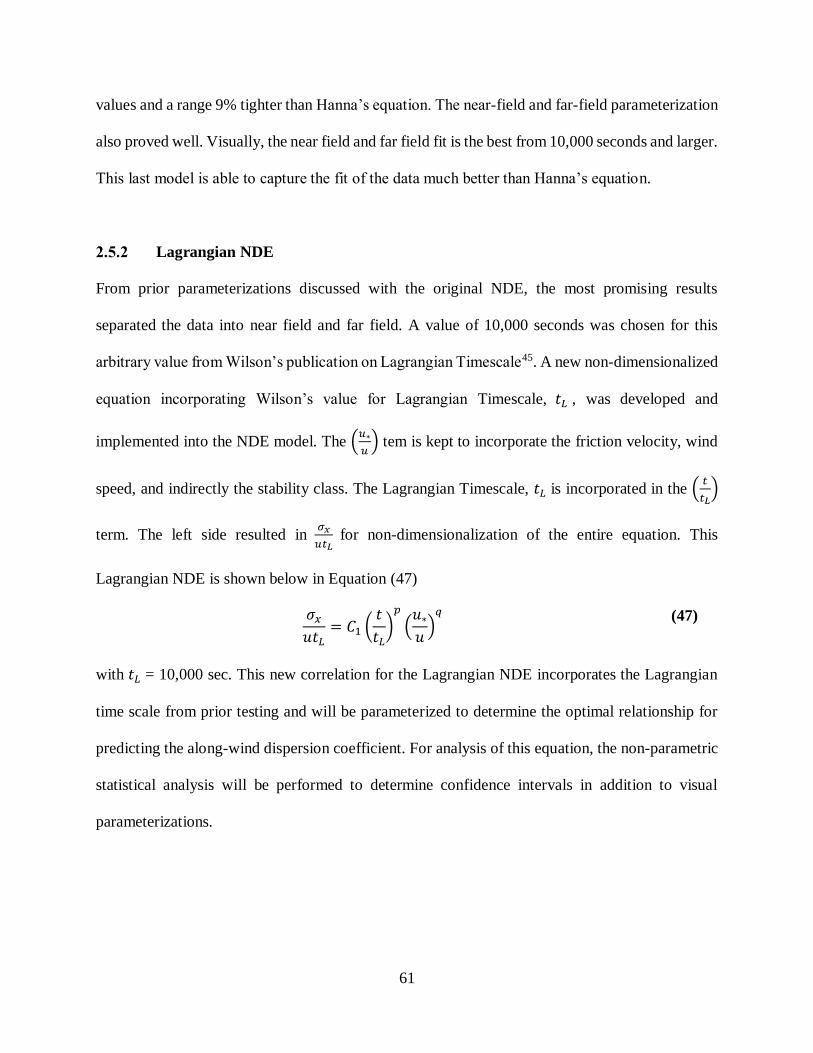
61
values and a range 9% tighter than Hanna’s equation. The near-field and far-field parameterization
also proved well. Visually, the near field and far field fit is the best from 10,000 seconds and larger.
This last model is able to capture the fit of the data much better than Hanna’s equation.
Lagrangian NDE
From prior parameterizations discussed with the original NDE, the most promising results
separated the data into near field and far field. A value of 10,000 seconds was chosen for this
arbitrary value from Wilson’s publication on Lagrangian Timescale45. A new non-dimensionalized
equation incorporating Wilson’s value for Lagrangian Timescale, 𝑡𝐿 , was developed and
implemented into the NDE model. The (𝑢∗
𝑢) tem is kept to incorporate the friction velocity, wind
speed, and indirectly the stability class. The Lagrangian Timescale, 𝑡𝐿 is incorporated in the (𝑡
𝑡𝐿)
term. The left side resulted in 𝜎𝑥
𝑢𝑡𝐿 for non-dimensionalization of the entire equation. This
Lagrangian NDE is shown below in Equation (47)
𝜎𝑥
𝑢𝑡𝐿= 𝐶1 (
𝑡
𝑡𝐿)
𝑝
(𝑢∗
𝑢)
𝑞
(47)
with 𝑡𝐿 = 10,000 sec. This new correlation for the Lagrangian NDE incorporates the Lagrangian
time scale from prior testing and will be parameterized to determine the optimal relationship for
predicting the along-wind dispersion coefficient. For analysis of this equation, the non-parametric
statistical analysis will be performed to determine confidence intervals in addition to visual
parameterizations.

62
2.5.2.1 All Data Sets
As an initial step, determination of the constants using all of the data was performed. The constants
from this parameterization are shown below in Table 16.
Table 15. Constants determined for Lagrangian NDE with all data
Constants All
p 1.01
q 0.66
C1 0.51
Total Tests 446
The constants prove similar to the original non-dimensionalized equation using all of the data. A
visual representation of the Lagrangian non-dimensionalized equation using all data is shown
below in Figure 18.
Figure 18. Time (s) vs. 𝝈𝒙
𝒖∗⁄ (s) as a function of the original data, Lagrangian NDE
predictions using all 446 data points, and Hanna’s predictions

63
Visually, the fit of the Lagrangian NDE is comparable to the original NDE shown in Figure 15.
All of the predicted data is below Hanna’s equation which fits the data better between 1,000 and
100,000 seconds but can be improved upon overall.
2.5.2.2 “Model” Data Sets
Determinations of the constants using only the “model” data of Marchwood, KitFox ERP, KitFox
URA, DTRA phase 1, Hanford, and Dipole Pride tests were performed with improvement seen in
the original NDE. The constants from this parameterization are shown below in Table 16.
Table 16. Constants determined for Lagrangian NDE with “model” data
Constants All Model
p 1.01 0.94
q 0.66 0.13
C1 0.51 0.10
Total Tests 446 63
The results of the Lagrangian NDE with “model” data shows smaller constants when compared to
the Lagrangian non-dimensionalized equation with all data. The constants determined with the
“model” data show that the terms on the right-hand side of the equation have less of an impact on
the along-wind dispersion coefficient as compared to all of the data. The Lagrangian NDE fit with
“model” data is shown below in Figure 19 to see a visual representation of the model validated
with “model” data.

64
Figure 19. Time (s) vs. 𝝈𝒙
𝒖∗⁄ (s) as a function of the original data, Lagrangian NDE
predictions using only “model” data points, and Hanna’s predictions
The Lagrangian non-dimensionalized equation with constants derived from “model” data shows a
better fit for the “model” data. The predicted data is observed to have different values for the same
time capturing the spread of data better. This spread of predicted data could not be achieved with
Hanna’s equation visually showing a better fit for the “model” data for along-wind dispersion.
2.5.2.3 “Model” Data Sets by Stability Class
As prior performed with the original NDE, parameterization by “model” data and stability class
was determined due to prior trends. The results from this parameterization are shown below in
Table 17.

65
Table 17. Constants determined for Lagrangian NDE with “model” data with stability class
All Data All “Model”
Data Model: A-C Model: D Model: E-G
p 1.01 0.94 0.75 0.93 1.20
q 0.66 0.13 1.03 0.96 0.76
C1 0.51 0.10 0.59 1.11 2.23
Total 446 63 30 12 21
From this parameterization, very noticeable trends appeared in the constants. An increase is shown
in the constant p as stability class transitions from the convective boundary layer to the stable
boundary layer. The constant q decreases over the same transition. C1 also increases over this
transition. A visual representation of the Lagrangian NDE by stability class compared with original
data can be seen below in Figure 20.
Figure 20. Time (s) vs. 𝝈𝒙
𝒖∗⁄ (s) as a function of the original data, Lagrangian NDE
predictions with “model” data points and stability class, and Hanna’s predictions
This graph shows only the “model” data with the Lagrangian non-dimensionalized fit using “model”
data by stability class. This NDE model shows an improved fit of the Lagrangian NDE

66
incorporating stability class. The deviation of the original data both above Hanna’s line and below
the line is able to be captured appropriately. The expansion of this equation to all of the available
data is plotted below in Figure 21.
Figure 21. Time (s) vs. 𝝈𝒙
𝒖∗⁄ (s) as a function of the original data, Lagrangian NDE
predictions with “model” data points and stability, and Hanna’s predictions
While the constants determined with the Lagrangian non-dimensionalized equation with “model”
data by stability class are a great fit for the “model” data, they are not a great fit for all of the data.
This equation is an improvement compared to Hanna’s equation as well as the original NDE due
to the spread of the prediction that fit the data both above and below Hanna’s prediction but can
be improved upon.
2.5.2.4 Summary of Lagrangian Non-Dimensionalized Equation
The Lagrangian non-dimensionalized equations proposed provides improvements on the overall
predictions for the along-wind dispersion coefficient. A non-parametric confidence interval was

67
chosen to evaluate the outcome of each model with 𝛼 = 𝜎𝑥(𝑝𝑟𝑒𝑑𝑖𝑐𝑡𝑒𝑑)
𝜎𝑥(𝑑𝑎𝑡𝑎) with optimal values closest
to 1. Shown below in Table 18 are the Lagrangian NDEs with their overall equations with constants,
90% confidence interval, and range of data.
Table 18. 90% Confidence intervals determined from non-parametric statistical analysis
Parameterization
(total tests)
Equation 90% Confidence
Interval
Range
Hanna (446) σx = 2u∗t 1.63 ≤ α ≤ 1.88 26%
Lagrangian NDE
(all - 446)
σx
utL= 0.51(
t
tL)1.01(
u∗
u)0.66 1.17 ≤ α ≤ 1.36 19%
Lagrangian NDE
(“Model” - 63)
σx
utL= 0.10(
t
tL)0.94(
u∗
u)0.13 0.99 ≤ α ≤ 1.14 15%
Lagrangian NDE
(“Model” by Stability
Class – 63)
𝜎𝑥
𝑢𝑡𝐿= 𝐶1(
𝑡
𝑡𝐿)𝑝(
𝑢∗
𝑢)𝑞 0.96 ≤ α ≤ 1.09
13%
The Lagrangian non-dimensionalized equation shows improvement when compared to both
Hanna’s equation and the original non-dimensionalized equation. The original NDE with constants
determined from all data is comparable to the Lagrangian NDE with constants determined from
all data. The effects of the equations start to differ when the constants are determined from both
“model” data and “model” data with stability class. The Lagrangian NDE has as a tighter range
for both “model” data and “model” data by stability class than the original NDE and Hanna’s
equation. The 𝛼 values are also closer to its optimal value of 1 with the Lagrangian NDEs
compared to the original NDE and Hanna’s equation.

68
Theoretical NDE
Similar to the Original NDE, the Theoretical NDE takes into account the friction velocity and time
twice whereas the Original NDE takes these parameters into account only once. The left side of
the equation is non-dimensionalized by these parameters instead of the distance in the original
NDE. This arrangement non-dimensionalized with the parameters discussed in the theoretical
derivations makes the equation slightly different than the original NDE. The overall theoretical
NDE is shown below in equation (48).
𝜎𝑥
𝑢∗𝑡= 𝐶(
𝑢∗
𝑢)𝑝1(
𝑢
𝑢𝑒)𝑝2 (48)
where p1, p2, and C are all dimensionless constants. Similar to the original NDE, the (𝑢𝑡
𝑥) or (
𝑢
𝑢𝑒)
term accounts for wind speed, u, time, t, and distance, x. The (𝑢∗
𝑢) term takes into account stability
class indirectly through wind speed and friction velocity. A multi-variable regression analysis was
performed with all of the data classified by stability class to determine the constants for C, p1, and
p2. The results of this analysis are shown below in Table 19.
Table 19. Values for C, p1, and p2 of theoretical NDE
Constants AB C D EF
C 0.034 0.460 0.238 0.071
P1 -1.262 -0.421 -0.706 -1.235
P2 -1.782 -0.0828 -0.652 -1.553
tests 5 24 40 20
From Table 19, all values of p1 and p2 are negative. All values of C are positive. Beyond being
negative or positive, there are no trends in the values within the constants. The predicted data with
this theoretical NDE is visually shown below in Figure 22.

69
Figure 22. Time (s) vs. 𝝈𝒙
𝒖∗⁄ (s) as a function of the original data by theoretical NDE and
Hanna’s predictions
Figure 22 shows 𝜎𝑥
𝑢∗⁄ vs. time for the original data, predicted data from the Theoretical NDE,
and Hanna’s equation. From the figure, many of the points are shown to overlap with the original
data. A statistical comparison of how the predicted data with the theoretical NDE and Hanna’s
equation are shown with MG VG values in Table 20.
Table 20. MG VG values for theoretical NDE
AB C D EF All
MG – NDE 1.000 0.935 0.958 0.928 0.946
VG – NDE 1.000 1.180 1.155 1.632 1.149
MG - Hanna 0.827 0.752 0.950 0.818 0.908
VG - Hanna 1.095 1.301 1.335 1.974 1.331
From Table 20, the theoretical NDE is an improved fit over Hanna’s equation for all stability
classes and overall data due to the MG and VG values being closest to 1. Overall, the theoretical
NDE classified by stability class is able to model the data better than Hanna’s equation based on

70
the visual representation in Figure 22 and MG VG values closer to 1 in Table 20. Although the
theoretical NDE performs better than Hanna’s equation, the input data can limit the use of the
theoretical NDE if it is not available, such as the effective wind speed, 𝑢𝑒.
Condensed NDE
The previous non-dimensionalized equations show improvement when compared to Hanna’s
equation. The major trends seen with the original NDE was an improvement when the time was
split into the near field and far field. This lead to the Lagrangian NDE. From the Lagrangian NDE,
the improvement was seen when “model” data was used with stability class. Another non-
dimensionalized equation was developed to incorporate both the trends in stability class and time.
A condensed non-dimensionalized equation has been developed to incorporate trends of stability
class or (𝒖∗
𝒖) and have all input parameters available. This condensed non-dimensionalized
equation is shown below in Equation (49)
𝜎𝑥
𝑢∗𝑡= 𝐶1(
𝑢∗
𝑢)p (49)
Where stability class is taken into effect with (𝒖∗
𝒖) term on the right hand side. 𝜎𝑥 as a function of
𝑢∗ and t is taken into account on the left hand side in this condensed non-dimensionalized equation.
“Model” data was used to develop the constants. A p-value was determined to be 0.995 due to the
averaged individual constants solved by “model” data and stability class for both 𝐶1 and p values.
The overall equation for the final NDE is shown below in equation (50)
𝜎𝑥
𝑢∗𝑡= 𝐶1(
𝑢∗
𝑢)0.995 (50)

71
Where 𝐶1 are the constants determined from each grouping of stability class, similarly performed
in all other NDEs. These values for constants are shown below in Table 21 with their respective
MG VG values.
Table 21. 90% Confidence intervals determined from non-parametric statistical analysis
Constants AB C D E FG All Hanna
𝑪𝟏 0.068 0.071 0.086 0.100 0.142 - -
p 0.995 0.995 0.995 0.995 0.995 - -
Total Tests 9 18 21 3 12 63 63
MG 0.916 0.905 0.995 1.001 0.966 0.953 0.850
VG 1.150 1.171 1.067 1.002 1.236 1.134 1.357
The trend observed with the constants show that as the stability class transitions from the
convective boundary layer to the stable boundary layer, the constant value increases. In Table 21,
the MG VG values for the “model” data are determined for Hanna’s equation, all of the “model”
data with stability class, and each of the individual stability classes. These MG VG values show
that each of the condensed non-dimensionalized equation’s predictions are better than predictions
by Hanna’s overall equation. A visual representation of the data predicted by the condensed NDE
is shown below in Figure 23.

72
Figure 23. Time (s) vs. 𝝈𝒙
𝒖∗⁄ (s) as a function of the original data by stability class, final
NDE predictions by “model” data with stability class, and Hanna’s predictions
This figure shows all of the model data with the original data, predicted data by the final non-
dimensionalized equation, and Hanna’s prediction. The condensed non-dimensionalized equation
by stability class is able to capture the trends evidenced in Figure 23 appropriately.
Final NDE
Throughout the analysis, data were checked and doubled checked to make sure all results are
consistent. OLAD-van tests were revisited and decided to be included in the final quality data to
be used in model validation. Note the OLAD-plane tests were still excluded due to their release in
the upper boundary layer. This inclusion of the OLAD-van tests resulted in a total of 89 tests to be
used as “validation” data for validating the constants. Kit Fox SSR tests were also accumulated at
this time, but not included in the validation data due to inconsistency in the data analysis. The
methods reported for determination of 𝜎𝑥 did not match with the values reported for 𝜎𝑥. A final

73
NDE was developed with the quality “Validation” data and is reported below in the final NDE
sections.
2.5.5.1 Additional Data for Model Validation and Trends in Stability Class
In addition to “validation” data inclusion, stability class was scrutinized. From previous NDEs
categorized by stability class, trends were seen in the constants for the respective stability classes.
This is expected because stability class is known to have an effect on atmospheric dispersion. To
see the effect of the stability class on the along-wind dispersion coefficient, the “validation” data
was color-coded by stability class. Overall trends in the original data by stability class are shown
below in Figure 24.
Figure 24. Time (s) vs. 𝝈𝒙
𝒖∗⁄ (s) as a function of the original data by stability class and
Hanna’s predictions
From Figure 24, noticeable trends are seen between the different stability classes. Stability Classes
AB and C do not have as steep of a slope as the line predicted by Hanna. Stability Class D spreads
out both above and below the line predicted by Hanna, but of the similar slope. Stability classes E
74
and F have a slightly steeper slope than the line predicted by Hanna. These trends show that the
stability class has an effect on the overall along-wind dispersion coefficient with respect to the
slope of the data trends. Stability class is taken into account with the (𝒖∗
𝒖) term. Determining a
constant as a function of the stability class is believed to be the most promising option and has
showed success with previous NDEs.
2.5.5.2 Final NDE by Stability Class
Figure 24 shows noticeable trends in the stability class. This supports the (𝒖∗
𝒖) term from the
theoretical non-dimensionalized equation. The (𝑢𝑡
𝑥) or (
𝑢
𝑢𝑒) term in the theoretical non-
dimensionalized equation accounts for wind speed, u, time, t, and distance, x. This term is not as
applicable due to the availability and predictability of the effective wind speed, 𝑢𝑒 . Due to
limitability of the effective wind speed and decreased impact of the effective wind speed, the (𝑢
𝑢𝑒)
term is removed from the equation resulting in the condensed NDE shown in Equation (51).
Although a term is excluded, the condensed NDE still shows improved modeling of the along-
wind dispersion coefficient. The quality “validation” data was used to determine the constants for
this final non-dimensionalized equation through a multi-variable regression analysis. An overall
value for the exponent was determined to be -0.5 due to individual constants with the validation
data. This new equation is shown below
𝜎𝑥
𝑢∗𝑡= 𝐶1(
𝑢∗
𝑢)−0.5 (51)
where values of 𝐶1 are determined for each stability class. With the OLAD-van data included in
the quality data, the constant changes from previous value determined with the condensed NDE
and 63 “model” data points. A single variable regression analysis is used with the data classified

75
into their respective stability classes and p = -0.5 to determine the values for 𝐶1. The values for the
constants as a function of stthe ability class are shown below in Table 22 with their respective
quantity of tests.
Table 22. Values for C1 with p = -0.5
AB C D E F All
C1 0.311 0.339 0.408 0.429 0.576 0.408
Tests 5 24 40 15 5 89
Table 22 shows clear trends in the 𝐶1 values as a function of the stability class when the p constant
is set to a value of -0.5. The trend observed with the 𝐶1 constant shows that as the stability class
transitions from the convective boundary layer to the stable boundary layer, the 𝐶1 value increases.
The average value of all of the tests for the constant 𝐶1 is 0.408. This 0.408 value is consistent with
a neutral stability class which aligns with models that use neutral stability if the stability class is
unknown. A visual representation of the final NDE classified by stability class is shown below in
Figure 23.

76
Figure 25. Time (s) vs. 𝝈𝒙
𝒖∗⁄ (s) as a function of the original data by stability class, final NDE
predictions classified by stability class, and Hanna’s predictions
Figure 25 shows the original data by stability class, predicted data by the final non-dimensionalized
equation classified by stability class, and Hanna’s prediction. This visually shows that this non-
dimensionalized equation is able to capture the trends evidenced in the stability classes
appropriately. A statistical comparison of how the predicted data with the NDE and Hanna’s
equation are shown with MG VG values below in Table 23.
Table 23. MG VG values for NDE by stability class with p = -0.5
AB C D EF All
MG – NDE 0.939 0.925 0.889 1.024 0.931
VG – NDE 1.096 1.240 1.178 1.458 1.248
MG - Hanna 0.728 0.713 1.011 1.217 0.942
VG - Hanna 1.234 1.418 1.296 1.484 1.365
Overall the MG VG values for all the validation data points are similar for both the final NDE MG
VG values and Hanna’s equations MG VG in Table 23. Classifying the data points into their

77
respective stability classes shows that the MG VG values for the NDE are able to model the data
more appropriately than Hanna’s equation. A parity plot is shown below in Figure 26 for another
representation of how the predicted data compares with the original data and shows how well this
NDE model collapses the experimental data.
Figure 26. 𝝈𝒙
𝒖∗⁄ (s) for the original data vs.
𝝈𝒙𝒖∗
⁄ (s) for the NDE by stability class for all of
the quality data with a reference line
Figure 26 shows that the predicted data falls along the reference line of what the data should be if
equivalent to the original data. The data is collapsed tighter between 0 and 10,000 seconds. There
is a bit larger spread of the data after 10,000 seconds. The final NDE by stability class does not
consistently over or under predicting the data which is good. Compared to Hanna’s equation,
shown in a parity plot in Figure 14, the final NDE by stability class is a better model due to the
tighter and more even distribution of the data points.

78
Overall, the NDE by stability class is able to model the data better than Hanna’s equation based
on the visual representation in Figure 25, MG VG values closer to 1 in Table 23, and collapse the
data better in the parity plot in Figure 26.
2.5.5.3 Final NDE by Stability with Monin-Obukhov Length
While the final NDE by stability class is a better fit than Hanna’s along-wind dispersion equation
and previous NDEs, it is believed it can be improved upon due to the trends observed in the C1
constants in Table 21. These trends show that as the stability class transitions from the convective
boundary layer to the stable boundary layer, the C1 value increases. This final proposed NDE takes
into account the Monin-Obukhov Length, λ, to model these trends. The final NDE was used as the
basis for the NDE with Monin-Obukhov Length. The final NDE is shown again in equation (52)
but with a different value for C1 shown in equation (53)
𝜎𝑥
𝑢∗𝑡= 𝐶1(
𝑢∗
𝑢)−0.5 (52)
𝐶1 = 𝐶𝑠/𝑐 − (𝐶𝑠/𝑐 − 𝐶𝑑 ) ∗ [exp (𝜆𝑠/𝑐
𝜆⁄ )]
(53)
where 𝐶𝑠/𝑐 and 𝜆𝑠/𝑐 are dimensionless constants. Equation (53) is able to make the 𝐶1 values a
function of the Monin-Obukhov length which directly relates to stability. Equation (53) is arranged
so that at a neutral boundary layer with a Monin-Obukhov length of 10,000, the constants cancel
out leaving the 𝐶1 value equal to 0.408. This value is consistent with the C1 value for stability class
D from Table 23. This arrangement allows for a smooth transition between the convective
boundary layer with negative Monin-Obukhov lengths and stable boundary layer with positive
Monin-Obukhov lengths. A smooth transition for all Monin-Obukhov lengths is desired from a

79
modeling perspective over individual stability classes. The values for the constants determined
from equation (53) with a multi-variable regression analysis are shown below in Table 24.
Table 24. Values for Cs/c and 𝝀𝒔/𝒄 constants with p = -0.5
Negative λ Positive λ D All
Cs/c 0.313 0.408 0.408
λS/C 186.360 -0.008
P -0.5 -0.5 -0.5
tests 32 51 40 83
Table 24 shows the constants for 𝐶𝑠/𝑐 and 𝜆𝑠/𝑐 for the convective and stable boundary layers.
There are not obvious trends in the data. The total tests show a slight decrease in amount compared
to the previous NDEs due to inclusion of the Monin-Obukhov length. Only 83 data points out of
the 89 included Monin-Obukhov length to account for this difference. A visual representation of
the Final NDE with Monin-Obukhov length predicted data is shown below in Figure 27.
Figure 27. Time (s) vs. 𝝈𝒙
𝒖∗⁄ (s) as a function of the original data, NDE predictions classified
by Monin-Obukhov Length, and Hanna’s predictions

80
Figure 27 shows the original data, data predicted with the final with Monin-Obukhov Length by
convective and stable boundary layer, and Hanna’s prediction. The slope of the NDE for a negative
Monin-Obukhov length is less than Hanna’s prediction which aligns with Figure 24 for unstable
stability classes or the convective boundary layer. The slope of the NDE for a positive Monin-
Obukhov length is greater than Hanna’s prediction which also aligns with Figure 24 for stable
stability classes. A statistical comparison of how the predicted data with the NDE and Hanna’s
equation are shown with MG VG values below in Table 25.
Table 25. MG VG values for NDE by Monin-Obukhov Length
Negative λ Positive λ All
MG – NDE 0.978 1.019 1.001
VG – NDE 1.247 1.318 1.286
MG - Hanna 0.785 1.117 0.957
VG - Hanna 1.446 1.424 1.433
The MG VG values for all of the data points in Table 25 are improved for the final NDE with
Monin-Obukhov Length compared to Hanna’s equation. Classifying the Monin-Obukhov length
by negative and positive values shows that the NDE has improved geometric means and geometric
variances compared to Hanna’s equations for both the convective and stable boundary layers. A
parity plot is shown below in Figure 28 for an additional visual representation of how the predicted
data with this NDE compares with the original data.

81
Figure 28. 𝝈𝒙
𝒖∗⁄ (s) for the original data vs.
𝝈𝒙𝒖∗
⁄ (s) for the NDE by stability class for all of
the quality data with a reference line
Figure 28 shows that the predicted data falls along the reference line of what the data should be.
The data is collapsed equally throughout all time. Compared to Hanna’s equation, shown in a
parity plot in Figure 14, the NDE with Monin-Obukhov length better predicts 𝜎𝑥 values compared
to Hanna’s equation due to the tighter grouping around 100 seconds and has more even distribution
of data points greater than 100 seconds.
Similar to the NDE by stability class, the NDE with Monin-Obukhov length is an improved model
based on the visual representation in Figure 27, MG VG values closer to 1 in Table 25, and collapse
of the data with the parity plot in Figure 28.

82
Summary
Multiple non-dimensionalized equations (NDEs) have been developed incorporating prior
derivations of the along-wind dispersion coefficient and available data. The theoretical NDE
provided improved predictions compared to Hanna’s equation, which is an improved fit for the
overall data. Although this NDE is visually and statistically better than Hanna’s equation, the
model itself is comprised of four separate equations based on stability class and requires the
effective wind speed, which may not always be available. Additional NDEs were developed
without the effective wind speed and classified by the stability class, labeled as the Final NDEs.
Both of these Final NDEs proved better than Hanna’s equation. The main difference between the
two final NDEs is whether or not Monin-Obukhov length is available. If the Monin-Obukhov
length is available, equations (52) and (53) are recommended to be used with values for constants
from Table 24. These equations provide one continuous NDE throughout all conditions. If Monin-
Obukhov length is not available, equation (51) is recommended with values for constants from
Table 21. Both of the Final NDEs are able to capture the spread of data better than Hanna’s
equation due to additional parameters and the inclusion of stability class.

83
Experimental Program

84
Introduction
An experimental program in the ultra-low speed wind tunnel at the Chemical Hazards Research
Center was established to determine an appropriate along-wind dispersion coefficient from the
concentration-time histories of finite-duration releases under different test conditions including
wind speed, release duration, distance downwind, and more. Descriptions of the equipment and
facility, experimental program, analysis, and results of the finite-duration releases are presented
below.
Equipment and Facility
The tunnel has a working section of 24 m in length with a 6.1 m x 2.1 m cross-section and wind
speeds from 0.34 m/s to 1.1 m/s. The LDV system allows for velocity profiles to be measured in
3 directions. A constant stress layer of 40cm produced with modified Irwin spire arrangement and
surface roughness ensures that all tests performed were within the constant stress layer. The FID
system also allows for concentration-time histories to be accurately measured. An area source
developed specifically for this program provides repeatable release durations at constant rates. All
of these capabilities provide an optimal testing facility for finite-duration releases. In this section,
the facility will be described as well as the equipment with necessary modifications.
Ultra-Low Speed Wind Tunnel
The Chemical Hazards Research Center houses an ultra-low-speed wind tunnel to model the
effects of hazardous gases in the atmosphere. The wind tunnel has a working section of 24 m in
length with a 6.1 m x 2.1 m cross-section. The wind tunnel has an established boundary layer of
60 cm and a constant stress layer of about 10cm with one layer of spires. The tunnel was designed

85
to run at wind speeds less than 2 m/s for scalability to atmospheric conditions, specifically for
denser-than-air gases but applicable for neutrally buoyant gases as well46. The wind tunnel is a
“push through” wind tunnel where the air is pushed through the working section in contrast with
many tunnels that are pull through. The tunnel is centrally located in the room with adequate
spacing on either side to provide uniform flow around and through the wind tunnel within the
isolated room. A control room adjacent to the wind tunnel provides observation and control of
equipment during testing without disrupting the flow. A floor plan of the wind tunnel with its
adjacent control room is shown below in Figure 29.
Figure 29. Floor plan of the wind tunnel at the CHRC47
In this floor plan, all tunnel characteristics discussed above can be seen. The symmetry of the wind
tunnel was found necessary for uniform flow in the tunnel. Not shown in the figure are three baffles

86
adjacent to the wind tunnel in alignment with the straightening section of the wind tunnel. These
baffles were tuned to ensure uniform flow distribution in the wind tunnel.
3.2.1.1 Fans and Air Flow
Two adjustable pitch vane-axial fans (Buffalo Forge Company Model 72D5 ADJUSTAX) built
by the Buffalo Forge Company are used to push air through the working section of the wind tunnel.
The 1.8 m diameter, 75 horsepower fans are controlled with a Fenner M-Trim speed controller
optimizing the master-and-slave method (Eaton Company DYNAMATIC Model VT-323). This
model uses eddy-current drives to control the speed of each fan within 0.5 % of the maximum
speed. Dolan-Jenner optical sensors were used to measure the fan rotation speed of each fan.
From the outlet of each fan, transition ducts carry wind from the circular output of the fans into a
rectangular input at the front of the wind tunnel. These ducts are comprised of 0.3 cm thick
polycarbonate plastic sheets connecting the end of the fan to the working section of the wind tunnel.
Honeycomb at the entrance of the wind tunnel provides a pressure drop of the flow for flow
straightening. This honeycomb has 1.2 cm cell size with 10.1 cm thick plastic-impregnated Kraft
paper. After the honeycomb, 4 seamless fiberglass screens are located at distances of 1.0 m, 1.1 m,
2.0 m, and 2.1 m downwind for additional flow straightening. After the air has passed through the
circular fans, rectangular input, honeycomb, and 4 screens, it is uniform and dispersed across the
full cross-section of the wind tunnel.

87
3.2.1.2 Boundary Layer and Surface Roughness
Fourteen Irwin spires placed at a distance of 30 cm downwind the last screen, were used to generate
a turbulent boundary layer. These spires are comprised of 0.36 cm thick acrylic and are 92.7 cm
in height, 13.2cm at the base, and 23.2cm in length as shown in Figure 30.
Figure 30. Drawing of Irwin Spires (left)47 and picture of Irwin Spires in wind tunnel (right)
Figure 30 shows the physical dimensions of the Irwin spires (left) and the physical placement of
the Irwin spires in the wind tunnel (right) with 46.3cm between each spire and 6.6cm between the
spires and the wall. The boundary layer is established through these Irwin Spires for a fully
developed boundary layer of 60 cm in depth after a distance of 6m downwind48. In addition to the
Irwin spires, aluminum angles were placed on the floor of the wind tunnel to provide a surface
roughness in the wind tunnel. The aluminum angles are 3.81 cm in height, width, and length with
an angle of 90⁰. They are placed at a spacing of 30.5 cm between the centers of each roughness
piece, using a template. A drawing showing the dimensions of each aluminum angle and their
physical distribution in the wind tunnel are shown below in Figure 31.

88
Figure 31. Physical placement of aluminum angles for surface roughness in wind tunnel
A turbulent boundary layer with a height of 10 cm was obtained using one layer of Irwin spires
and aluminum angles. The boundary layer is considered fully developed 6 m downwind of the 1
m tall spires. The remaining portion of the wind tunnel downwind of this boundary layer generation
region served as the working section of the tunnel.
3.2.1.3 Validation of Uniform Flow (Visual)
Flow is expected to be uniform through the wind tunnel, but some variation was observed. Flow
around the tunnel is desired because of building constraints which have an effect on flow in the
tunnel. To achieve uniform flow in the wind tunnel, three baffles were installed on the starboard
side of the wind tunnel in alignment with the straightening section. The angles in which these
baffles were positioned needed to be determined for uniform flow in the wind tunnel. Validation
of the uniform flow was visually achieved using a water-based fog solution fed through a Rosco
1500 fog machine and house-made fog chiller into PVC piping through the center of the wind
tunnel directly behind the Irwin spires from a point source. Black plastic was fixed on the floor of
the wind tunnel floor for improved visualization of the white smoke. Blue painters tape was
secured to the black plastic in 61 cm x 61 cm increments for quantified visualization. Multiple

89
arrangements of the three baffles at different angles were tested to achieve uniform flow through
video taken in the wind tunnel. A screenshot of uniform flow is shown below in Figure 32.
Figure 32. Uniform flow in the tunnel with fog and black plastic on the floor for visualization
Figure 32 shows that the flow injected at the center of the wind tunnel is relatively uniform from
a visual perspective throughout the wind tunnel. Subsequently, all other tests conducted in the
wind tunnel were done using this configuration. To further validate the uniform distribution of the
flow, velocity profiles were measured which will be discussed in a later section.
3.2.1.4 Wind Speed and RPM relationship
The relationship between fan speed in rotations per minute (RPM) and average velocity at the
height of 40 cm was determined through prior experimental work shown below in Figure 33.

90
Figure 33. The relationship between velocity in the wind tunnel at the height of 40cm and
fan speed in rotations per minute (rpm).
From Figure 33, the relationship between the fan rotations and wind speed in the tunnel is shown
to be relatively linear. This relationship was used as a general guideline to set the fan speeds for
consistent velocity. These experiments were conducted using fan speeds of 90 and 50 RPM for
free stream velocities of 0.71 m/s and 0.35 m/s, respectively at the height of 60 cm.
3.2.1.5 Traverse System
An existing traverse system installed on the ceiling of the wind tunnel was used to remotely place
instruments at appropriate positions including Hot Wire Anemometer (HWA), Laser Doppler
Velocimeter (LDV), and Flame Ionization Detector (FID) within the wind tunnel. In the present
experiments, the atomizer, HWA, LDV, and FID were respectively mounted on arms 1, 2, 3, and
4. Each arm houses a micro-electric motor to move the machine mounted at the end of each arm

91
in the x-, y-, and z-direction. All positions of the arms were controlled remotely from the control
room with numerical values indicated on display within the control room.
Area Source
Ground level releases were chosen for these tests for direct application in modeling. For the
experiments within this project, an area source was developed for finite-duration releases to
improve understanding of the effects of along-wind dispersion. The design and implementation of
the area source are discussed below.
3.2.2.1 Design of Preliminary Area Source
A 0.31 m x 0.31 m x 0.31 m (L x W x H) area source was created for the finite-duration experiments.
In the preliminary prototype, three sides and the bottom were made out of wood one side was made
of a polycarbonate sheet for visualization. The top of the box was comprised of cold-rolled steel
with 23% perforated holes. The box had 3 mixing layers of 23% perforated sheets at heights of 7.6
cm, 15.2 cm, and 22.9 cm from the bottom of the box to ensure adequate mixing of the incoming
gas from the bottom. For visibility during preliminary testing, 4 strips of white LED 12V lights
(MPJA light strip model 31364 OP) were attached to 0.3 cm metal rods that were suspended
through holes drilled in the sides of each box. These light/rod combinations were placed across the
back of the box at a distance of 5 cm from the back edge. The heights of the lights were at 3.8 cm,
11.4 cm, 19 cm and 26.7 cm for ample lighting between the mixing layers. The tape was used to
seal the holes suspending the light / rod combinations to provide a well-sealed box.

92
3.2.2.2 Visual Testing of Mixing of Area Source
Visualization tests were performed with Rosco water-based fog fluid fed through a Rosco 1500
fog machine at the lowest setting of 1, into 2.4 m length of dryer duct with a 7.6 cm diameter. The
dryer duct was fed into the 7.6 cm diameter entrance hole at the bottom of the box. Various
combinations of the plates were tested to determine equal spreading of the fog across the 0.31 m
x 0.31 m area source. The tests were performed with various arrangements of the mixing plates
and an arrangement with a 15.2 cm x 15.2 cm centered blockage on the 7.6 cm plate. In tests, it
was apparent that the box filling time was significant to the uniform flow at the outlet of the box.
Figure 34 shows a uniform layer of fog leaving the top of the source box with well-mixed fluid
inside the box. This configuration was used in the final source box fabricated from aluminum.
Figure 34. Screenshot of video to show well-distributed flow through preliminary area source
3.2.2.3 Concentration Testing of Mixing of Area Source
After flow visualization was performed on the area source, a 500 ppm propylene and tank air
mixture was fed into the bottom of the box for concentration measurements. Concentration

93
measurements were done with a miniPID (Aurora Scientific model 200b) that had no modifications
performed. After calibration was performed on the machine, concentration measurements were
made at 7.6 cm increments throughout the entire box. Uniform concentration was measured at each
test point. After the aluminum box was created, visual releases were performed, and concentration
was measured with the fastFID. All results showed a uniform distribution of concentration across
the area source.
3.2.2.4 Creation of Permanent Area Source
After preliminary testing of the wooden box was complete, an aluminum version of the box was
made with the same mixing design as the preliminary wooden box. The top of the box was
modified from the preliminary area source to allow for a controlled release of the source gas. This
modified top was comprised of 2 sheets of cold rolled steel with 23% perforated holes and a sheet
of polypropylene with 23% perforated holes between the two metal sheets. This design allows for
the polypropylene middle sheet to be moved pneumatically between the two metal sheets to open
and close the holes when aligned and misaligned, respectively, to allow for finite-duration releases
of the source gas through the top of the area source. The box was secured into the wind tunnel at
a distance of 20 ft downwind, and 10 ft crosswind (or centerline), with the top of the area source,
mounted flush with the floor. When the top of the box is closed, slots in two the sides of the box
are opened for the source gas to be vented under the floor of the wind tunnel allowing for a
continuous release of the source. This configuration allows the mass flow meters providing the
source gas for operating at a constant rate which eliminated issues that can be encountered if the
mass flow meters are stopped and started.

94
3.2.2.5 Automation of Permanent Area Source
The area source was automated with a 120V 5-valve solenoid valve, Arduino Uno, and relay board.
House air was fed at 60psi into 3/8” tubing under the wind tunnel to pneumatically control the area
source through the solenoid valve. The 60psi house air was connected to the input of the solenoid
valve to 1) open the top of the area source while shutting the ventilation sides or 2) close the top
of the area source while opening the ventilation sides. The solenoid valve was operated from the
control room through the relay board, Arduino, and computer recording data. The Arduino
software also allowed for the release duration to be accurately controlled for any release duration
desired. Virtual clicker software synchronized the capture of data with the release of source gas.
Concentration testing
Concentration can be measured effectively by different methods. Two common machines to
measure the concentration of atmospheric releases are Flame Ionization Detectors (FID) and Photo
Ionization Detectors (PID). Both machines are non-specific detectors using an energy source to
form ions and record the amount of ions detected. A discussion of the two concentration
measurement apparatus is presented below.
3.2.3.1 Fast Flame Ionization Detector (FID)
A Cambustion HFR-400 Atmospheric fast Flame Ionization Detector (FID) was the main
equipment used for concentration measurements in the wind tunnel at the Chemical Hazards
Research Center. The FID system utilizes a hydrogen flame to burn a hydrocarbon traced sample
through a capillary tube inside the instrument. Ions are detected with a metal high DC voltage ion
collector. The schematic of the fastFID system is shown below in Figure 35.

95
Figure 35. Schematic of fast FID 49
The current produced by the high voltage ion collector is proportional to the rate of ionization
which is dependent on the concentration of hydrocarbons being sampled. The FID is a non-specific
aspirated probe that utilizes propane, in these tests, as the source tracer gas for concentration
measurements. Known concentrations of propane were used to calibrate the FID. A basic
calibration plot is shown below when first testing the fastFID.
Figure 36. Concentration (ppm) vs. Signal plot for Propane with the fastFID system
0.95
1
1.05
1.1
1.15
0 200 400 600 800 1000
Ave
age
Vo
ltag
e (V
)
Propane (ppm)

96
Early in the test program, variation in the voltage during calibration was much larger than expected
shown in Figure 36. Expanding on the variations, Figure 37 shows the voltage as a function of
time where the level of variability is unacceptable for a transient experiment.
Figure 37. Time vs. signal plot for multiple concentrations of propane using the FID system
After an extensive investigation, the unstable signals shown above were found to be due to
inadequate mixing of the propane and air from the mass flow meters. A Koflo Stratos static mixer
was installed in the gas lines used during calibration and experiments. In addition to the mixer, the
mass flow meters were mounted to a single metal block to reduce the delay when changing
concentrations levels during calibration. These additions improved the delivery of gasses
producing an acceptable calibration curve shown below.
0.96
0.97
0.98
0.99
1
1.01
1.02
1.03
1.04
1.05
0 0.5 1 1.5 2 2.5 3
Vo
ltag
e (V
)
Time (minutes)
43 ppm
129 ppm
240 ppm
343 ppm
429 ppm

97
Figure 38. Calibration curve of propane with fast FID
With these changes, the fastFID signal during calibration was stable and linear as shown in Figure
38. The standard deviation of each signal varied from 1.2 mV at 0.15% C3H6 to 7 mV at 1% C3H6.
3.2.3.2 Mini PhotoIonization Detector (miniPID)
Before the unstable signal associated with the FID was determined to be a mixing problem, an
Aurora Scientific miniPID model 200b was purchased. The miniPID is similar to the FID in that
it is an aspirated probe using a nonspecific ion detector. The main difference between the PID and
FID is that a PID uses a lamp for the energy source where the FID uses a hydrogen flame. The PID
is able to ionize compounds with ionization energy less than the lamp power. The pathway of gas
sampling through the PID is similar to the FID and is shown below in Figure 39.
0.000
0.500
1.000
1.500
2.000
2.500
3.000
0 0.2 0.4 0.6 0.8 1 1.2
Vo
ltag
e (V
)
% of C3H6

98
Figure 39. Schematic of PID50
From Figure 39, the flow of a sampled gas enters the probe where it passes between two plates.
The ions generated by the lam are measured and produce a voltage proportional to the ions
produced. The miniPID was modified so that the intake volumetric flowrate matches the area of
the probe inlet. This was performed with various chokes on the vacuum line behind the head of
the miniPID. Appropriate flow rates were obtained so that the sample velocity was roughly equal
to the expected wind speed at the measurement height. Unfortunately, this resulted in time delay
issues with the measurements.
3.2.3.3 Comparison of Signals from FID and PID
The decreased flow rates caused a time delay within the miniPID. A period of >3 minutes was
required for the miniPID before stable signals could be achieved. For non-choked flow, a period
of 1 minute was needed before the miniPID produced stable readings. Both 1 minute and 3 minute
periods between introduction of sample and a stable reading were unrealistic to be used for the
finite-duration tests. Figure 40 compares the response of the miniPID and fastFID.

99
(a) (b)
Figure 40. Concentration as a function of time for the miniPID (a) and the fast FID (b)
The signal to noise ratio with the miniPID during this stabilization period is about 10-20% of the
signal where the FID has a random signal to noise ratio of <1%. Based on this comparison, the
fastFID was used in the experiments.
Mixing of Gases
The accuracy of the concentration depends on the accuracy of the equipment and release of gases
into the wind tunnel. As mentioned in the fastFID section, accurate delivery of gasses was
improved based on modifications made.
3.2.4.1 Calibration of Mass Flow Controllers (MFC)
A 5 LPM MKS G-series Mass Flow Controller was used for propane in addition to a 20 LPM MKS
1559A Mass Flow Controller for house air. The 5 LPM and 20 LPM MFCs were calibrated using
a purpose-built apparatus shown in Figure 41.

100
Figure 41. Calibration apparatus for 5 lpm and 20 lpm MFC using positive displacement
A 5.313 L Plexiglas box initially filled with water. The time to fill the inner box is recorded to
determine the flow rates of the 5 LPM and 20 LPM mass flow controllers using displacement with
air. The inner box is manually lifted on a pulley system as gas fills the inside to keep the water
level inside and outside of the box equivalent. The corrected flow rates for the MFCs are shown
below in Table 26 where y is the output on the MFC with the correction applied, and x is the input
value on the MFC to achieve the desired output.
Table 26. Corrected flow rate equations for mass flow controllers
MFC Corrected flow rate equations for MFCs
5 LPM 𝑦 = 1.0377𝑥
20 LPM 𝑦 = 1.0088𝑥 + 0.0108

101
In addition to the corrected flow rate equations shown in Table 26, the input values were adjusted
for daily temperature T and pressure P using the ideal gas law. The MFCs were controlled by an
MKS Model 647B Multi-Gas Controller. All flow rates of gases were adjusted for the corrected
flow rate through calibration and the daily temperature and pressure in the room for increased
accuracy.
3.2.4.2 Connection of Gases
The connection from mass flow controllers to the mixing apparatus was observed to have a time
delay associated with the 5 SCCM MFC that was used with the miniPID. With low flow rates such
as 5 SCCM, this length can add an hour to the time the gases are turned on until a well-mixed flow
is achieved. A solid aluminum block with standard pipe fitting tapped holes was used as the
connection site for up to 5 mass flow controllers to decrease the time delay associated with lower
flow rates as shown in Figure 42.
Figure 42. The connection of mass flow meters used in tests

102
The dimensions of the aluminum box are 11.4 cm x 5.7 cm by 5cm with four 1/8” threaded holes
on the longer edges of the box to accommodate the standard MFCs, a 3/8” threaded hole at the end
for larger MFCs, and a 1/4” threaded hole at the head of the box for outlet flow to be fed into a
static mixer. When an MFC was not connected, plugs were used to seal the threaded holes. The
aluminum box drastically decreased the dead time between the output of the MFC and the mixing
apparatus from 1 hour to almost instantaneous flow to the mixing apparatus.
3.2.4.3 Mixing of Gases
From the aluminum box, the gases flow straight into a Koflo Stratos static mixer with 32 helical
mixing elements within the 3/8” OD metal tube. The design of the Koflo Stratos static mixer is
shown below in Figure 43.
Figure 43. Koflo Stratos static mixer51 used in the gas setup
The new apparatus ensures adequate mixing by the 32 helical mixing elements.
3.2.4.4 Additional Mixing of Gases with Dead Space
At low concentrations, a sinusoidal signal was observed on an oscilloscope. Gases were proven to
be well mixed at higher concentration. The mass flow controllers were observed to be fluctuating
in their output causing the sinusoidal signal. Dead space was created with a 2 L volume with metal
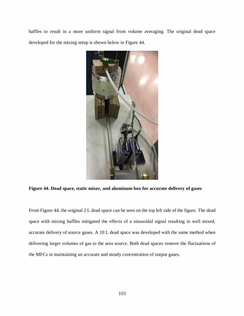
103
baffles to result in a more uniform signal from volume averaging. The original dead space
developed for the mixing setup is shown below in Figure 44.
Figure 44. Dead space, static mixer, and aluminum box for accurate delivery of gases
From Figure 44, the original 2 L dead space can be seen on the top left side of the figure. The dead
space with mixing baffles mitigated the effects of a sinusoidal signal resulting in well mixed,
accurate delivery of source gases. A 10 L dead space was developed with the same method when
delivering larger volumes of gas to the area source. Both dead spaces remove the fluctuations of
the MFCs in maintaining an accurate and steady concentration of output gases.

104
3.2.4.5 Results of the new mixing of gases
When gas is fed from the cylinders to the mass flow controllers, through the aluminum box, static
mixer, and dead space, accurate and well-mixed gases are produced. Concentration measurements
of propane were retested with the FID to check the stability of the signal and are shown below in
Table 27.
Table 27. Concentration testing of FID with propane after modifying the mixing setup
Propane % average (V) max (V) min (V) Range % Stand. Dev (V)
1 2.555 2.583 2.529 2.0% 0.006
0.75 2.227 2.249 2.205 2.0% 0.005
0.5 1.871 1.890 1.856 1.8% 0.004
0.25 1.474 1.484 1.462 1.5% 0.003
0.15 1.295 1.306 1.282 1.9% 0.003
0 0.983 0.986 0.979 0.7% 0.001
The average voltage, maximum voltage, and minimum voltage measured for a known
concentration of propane are shown above in Table 27. In addition to the voltages, the ranges of
the variation in signals and their standard deviations were also recorded and show the consistent
and accurate delivery of gases.
Laser Doppler Velocimetry (LDV)
A Laser Doppler Velocimetry (LDV) system is a non-intrusive velocity measurement system
projecting monochromatic, coherent lasers into fluid flow seeded with particles. The reflection of
laser light by the particles causes a Doppler shift in frequency that is proportional to the velocity
of the moving, illuminated particles. The Doppler shift is the difference between frequencies. The
velocity is then determined by analyzing the frequency of the signals.
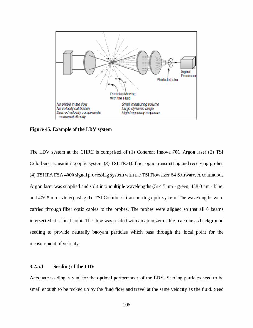
105
Figure 45. Example of the LDV system
The LDV system at the CHRC is comprised of (1) Coherent Innova 70C Argon laser (2) TSI
Colorburst transmitting optic system (3) TSI TRx10 fiber optic transmitting and receiving probes
(4) TSI IFA FSA 4000 signal processing system with the TSI Flowsizer 64 Software. A continuous
Argon laser was supplied and split into multiple wavelengths (514.5 nm - green, 488.0 nm - blue,
and 476.5 nm - violet) using the TSI Colorburst transmitting optic system. The wavelengths were
carried through fiber optic cables to the probes. The probes were aligned so that all 6 beams
intersected at a focal point. The flow was seeded with an atomizer or fog machine as background
seeding to provide neutrally buoyant particles which pass through the focal point for the
measurement of velocity.
3.2.5.1 Seeding of the LDV
Adequate seeding is vital for the optimal performance of the LDV. Seeding particles need to be
small enough to be picked up by the fluid flow and travel at the same velocity as the fluid. Seed

106
particles need to be neutrally buoyant to accurately track the flow without buoyancy effects adding
to the velocity in the vertical direction. If denser-than-air effects are seen, the LDV will pick up
the downward motion of the particle as the downward velocity. The seed particles need to be
injected non-invasively into the flow rate to avoid disruption of flow upwind. If a large object is
directly upwind of the flow, bluff body effects will be measured by the LDV instead of true
velocity in the wind tunnel. Lastly, seeding material needs to be non-toxic due to exposure in the
facility. Two pieces of equipment used for seeding will be discussed further: atomizer and fog
machine.
3.2.5.1.1 Atomizer
A TSI Model 8320 Atomizer was used primarily for seeding of the LDV system. The atomizer had
a house supply of air fed to the atomizer at 80psi. The initial design of the atomizer had a straight
outlet tube which provided seeding directly above the atomizer. This was not a desirable
configuration for seeding down to the floor of the wind tunnel. Consequently, a new outlet tube
was created using curved flexible tubing secured to a ¼ cross-section of a 3” PVC pipe 2.5 cm in
thickness. A larger diameter tube was then attached to the flexible tubing projected parallel to the
floor from the atomizer body. This modification allowed for the spread of seeding to reach the
floor for velocity measurements at low heights and can be seen in Figure 46.

107
Figure 46. TSI Model 8320 Atomizer with outlet tube modifications for optimal seeding
The modified atomizer was placed 0.24 m upwind, 45 cm crosswind, and at the same height of the
LDV to provide adequate seeding and not cause bluff body effects. This distance provided ample
seeding for the LDV for preliminary tests. The atomizer was filled with a 50% glycerin and 50%
deionized water by volume ratio. This solution had been pre-mixed for 1 hour in an ultrasonic
agitator before use in the atomizer to ensure a uniform solution. For wind speeds of <1 m/s, the
seeding was observed to be “slumping” towards the ground before it reached the LDV 0.24 m
downwind. This phenomenon was presumed to be the result of the presence of large droplets
expressed in the non-dimensional Weber number52, We
𝑾𝒆 =𝝆𝒗𝟐𝒍
𝝈
(54)
Where 𝜌 is the density (kg/m3), v is the velocity (m/s), l is the characteristic length (or droplet
diameter) (m), and 𝜎 is the surface tension (N/m). With the glycerin being dense, this parameter
was unable to be changed. To decrease the surface tension, a surfactant was added to the seeding
solution. 1-Butanol was chosen due to its long hydrocarbon chain and evaporation properties.
Molarities of 0.1-1M were tested in the glycerin-water solution. The molarity of 1M showed no
denser-than-air effects on the plume and was used for all LDV testing using the atomizer.

108
3.2.5.1.2 Fog Machine
Previous LDV tests performed in 2001 at the CHRC used a Rosco 1500 fog machine filled with
Rosco fog fluid (propylene glycol and deionized water) resulted in seeding rates of 1000Hz with
the LDV in coincidence mode for 2D measurements53. In a bid to replicate such high seeding rates,
3 fog machines were tested: Rosco 1500, Rosco PF-1200, and a Virhuck 400W machine.
Modifications to the machines were undertaken to allow for continuous delivery of fog and control
of the releases from the control room. In addition to the flow, different solutions were tested: Rosco
Fog Fluid, Froggy’s Fog Cryo Freeze, Froggy’s Fog Fast Dissipating, Chauvet DJ FJ-U, and
multiple homemade solutions of glycerin in DI water (50%, 25%, and 12.5%). While glycerin in
DI water produced the thickest smoke, a slippery residue is left. Propylene glycol was found in the
SDS’s of all manufactured solutions. Different compositions of propylene glycol and DI water was
tested until it was found that high concentration of this solution caused difficulty breathing and
destroyed contact lens. These results are consistent with exposure of non-asthmatics to propylene
glycol mist resulting in decreased tears, increased ocular and throat symptoms, decreased forced
vital capacity, and cough54.
Different configurations for the delivery of the fog fluid was tested. Three configurations that were
analyzed: 1) direct delivery of fog from the machine, 2) delivery of fog from the machine through
0.24 m of 7.6 cm aluminum dryer duct, and 3) delivery of fog from the machine through 0.24 m
of 7.6 cm aluminum dryer duct submerged in an ice bath. The different configurations for delivery
have an effect on the temperature fog which results in a change in the density of the fog. A
comparison of the 3 delivery mechanisms of 50% glycerin and 50% DI water solution are shown
below in Figure 47.

109
Figure 47 Delivery of 50% glycerin solution with no dryer duct (left), with dryer duct
(middle), and with dryer duct submerged in ice (right)
The delivery mechanisms have a large effect of the fog seeding and density as shown above in
Figure 47. Delivery of fog without a fog chiller or dryer duct was shown to provide the most
diluted but most dispersed cloud. Delivery of fog through a fog chiller with and without ice
provided a more dense cloud. While delivery of fog through a fog chiller provided denser seeding,
they had denser than air effects which are not desired with the LDV. A delivery of 50/50
glycerin/water solution was chosen due to its neutral buoyancy and non-toxic properties. This fog
was flooded in the entire wind tunnel to remove entrainment effects when directly injected upwind
of the wind tunnel. While this method provided great seeding, a thorough cleaning of the wind
tunnel needed to be performed after all velocity profiles were measured. The seeding of the
entirety of the wind tunnel flow was required when measuring increased turbulence observed with
multiple rows of spires.

110
3.2.5.2 Mounting and Alignment of the probes
All six beams produced from the Colorburst system of 3 frequencies (blue, green, and violet)
needed to be aligned for 3D measurements through a 100-micrometer hole. To measure the
velocities within 0.5cm to the floor, the probes were mounted at angles of ~54⁰ (blue and green
probe) and ~12⁰ (violet probe) so that the focal point of all of the lasers could reach the floor. LDV
measurements are typically made with each probe normally mounted at a 90˚ angle with respect
to the flow. The TRx10 fiber optic probe projected blue and green beams, so any alignment issues
had to be repaired by the manufacturer. The violet probe, however, was separately mounted and
needed to be aligned with the focal point of the blue and green probe. The configuration of the
probes is shown below.
Figure 48. Alignment of probes with their respective angles of α for the green and blue probe
and β for the violet probe
α β

111
The alignment procedure was performed with a 100-micrometer diameter aperture. The power of
each beam was measured at the output of the 100-micrometer hole to ensure that full beams were
projected during alignment.
3.2.5.3 3D flow
LDV systems are able to measure flow in single or multiple directions depending on the angle of
the probe. In particular, if three frequencies are produced with three pairs of beams, as in the testing
arrangement, the LDV is capable of measuring velocity in three directions. Coincidence mode in
the software was enabled for the tests. This allowed for 3D velocities of the particle to be measured
simultaneously, allowing for properties such as Reynolds stress or friction velocity to be obtained
from the measurement of flow. If a particle was not measured by all of the beams, it was not
recorded resulting in more accurate velocity measurements.
3.2.5.4 Matrix Transformation
To account for corrections in the direction from 90˚ to the angles mounted in the probe
arrangements, a transformation matrix was applied in the software. The projection of the matrix
with respect to the angles of the probes provides the adjusted velocity measurements in the x-, y-,
and z-direction. The transformation for the 3D LDV system at the CHRC is shown with theoretical
and numerical values in Figure 49.

112
Figure 49. Theoretical55 (left) and numerical (right) values for the matrix transformation for
the LDV mounted at angles
From the numerical values shown in Figure 49, the full velocity in Channel 1 (green beams) is
contributing to U (velocity in the x-direction). The measured velocities from Channel 2 (blue
beams) and Channel 3 (violet beams) are split between V and W (velocities in the y- and z-
direction respectively) due to their angles. The software measures the velocities of each channel
and then transforms the velocities to account for the angles in which they are mounted with the
transformation matrix to produce accurate transformed 3D velocity measurements.
Testing of this transformation matrix was performed comparing all velocities and turbulence
intensities reported with the transformation matrix applied in the software to values measured
solely by one pair of frequencies at a 90˚ angle with no correction. During this comparison, the
violet probe was shown to be unusable. A new transformation matrix was applied with the blue
beam measuring both the y- and z-direction with the sin(α) and cos(α) respectfully. After this
transformation matrix was applied, the values at an angle still did not match the values measured
at 90˚. An error in the manual was found. Performing the inverse of the transformation matrix to
the data measured at an angle was shown to provide the same values as measured at 90˚. The TSI
Flowsizer was unable to process this. The inverse of the transformation matrix for 2 beams
resulting in 3D velocity measurements required Matlab for data processing.

113
3.2.5.5 Flowsizer 64 Software Settings
The Flowsizer 64 software measures and analyzes the frequencies transmitted from the probes and
their backscatter through a signal processor to determine the correct velocities for each channel.
The software is a function of its inputs, so accurate input conditions are vital to accurate outputs.
The input conditions for the tests performed are described below in the hardware and software
settings.
3.2.5.5.1 Hardware Settings
The hardware settings specify the correct parameters associated with the laser and the fiber optic
probes, such as frequencies, distances, sizes, etc. In the hardware settings, the channels enabled
can be selected for 1, 2, or 3D measurements. The transformation matrix, described above, is
implemented in the hardware settings to correct for the angles of the probes. Information about the
specific probes used is input into the hardware settings such as wavelength, focal length, beam
separator, laser beam diameter, beam expander, fringe spacing, Bragg cell, and diameter sizes. In
this configuration, TSI TRx10 fiber optic probes were used. Optic settings for the system are
shown below.

114
Figure 50. Optimal Hardware settings for Optics in Flowsizer 64 software
From Figure 50, the specified values for each of the settings are shown. These values were obtained
from the TRx10 fiberoptic probe manual, Coherent Innova 70C Laser manual, and physically
measured for the setup within the wind tunnel. The settings input into the hardware are all a
function of the equipment used and how it is physically aligned.
3.2.5.5.2 Software Settings
The software settings in the Flowsizer 64 Software consist of the PMT voltage, Burst Threshold,
Band Pass Filter, Signal to Noise Ratio, Downmixing Frequency, Gate Scale, and Subranges. The
software settings are less concrete in comparison to the hardware settings in which they are
dependent on the overall system and not individual measured values. To determine the optimal
values for each setting, trial and error are required. The optimal settings for the LDV configuration
in the wind tunnel at the CHRC at 90RPM are shown below in Figure 51.

115
Figure 51. Optimal Software settings for LDV controls in Flowsizer 64 software
Optimal settings were determined by comparing, the data rate, burst efficiencies, and Gaussian
distributions to ensure that they compare to the values recommended by the manufacturers for
quality and reliable measurements. Gaussian distributions of the velocity or frequency versus valid
count for all channels are desired. An example of the Gaussian distributions achieved is shown
below in Figure 52.

116
Figure 52. Results of velocity measurements from optimal software settings
From Figure 52, Gaussian distributions are achieved for the velocities and frequencies for channels
1, 2 and 3. This shows that the settings chosen are of optimal values to produce accurate velocity
measurements.
3.2.5.6 Analysis of the Velocity Measurements
Transformed velocities obtained from the processor matrix as a function of time, were exported
from the Flowsizer 64 software. These values were analyzed within Matlab for their respective
sample size with the following equations56. The instantaneous, transformed values for velocities
were exported from the Flowsizer 64 software and are referred to below as 𝑈𝑖, 𝑉𝑖, and 𝑊𝑖 for the
x, y, and z instantaneous velocity directions respectively. The mean velocities in each direction,

117
U, V, and W, are solved as a function of the instantaneous velocities for the sample size, N, in
equations (55) - (57).
𝑼 = 𝟏
𝑵∑ 𝑼𝒊
𝑵
𝒊=𝟏
(55)
𝑽 = 𝟏
𝑵∑ 𝑽𝒊
𝑵
𝒊=𝟏
(56)
𝑾 = 𝟏
𝑵∑ 𝑾𝒊
𝑵
𝒊=𝟏
(57)
The turbulent components associated with each velocity, u, v, and w, are solved as a function of
the instantaneous velocities and their deviation from the mean velocities for each test with
equations (58) - (60).
𝒖 = [𝟏
𝑵∑(𝑼𝒊 − 𝑼)𝟐
𝑵
𝒊=𝟏
]
𝟏𝟐
(58)
𝒗 = [𝟏
𝑵∑(𝑽𝒊 − 𝑽)𝟐
𝑵
𝒊=𝟏
]
𝟏𝟐
(59)
𝒘 = [𝟏
𝑵∑(𝑾𝒊 − 𝑾)𝟐
𝑵
𝒊=𝟏
]
𝟏𝟐
(60)
The correlation between the turbulent components u and w is shown with 𝜌𝑢𝑤 below.
𝝆𝒖𝒘 = (𝑼𝒊 − 𝑼)(𝑾𝒊 − 𝑾)̅̅ ̅̅ ̅̅ ̅̅ ̅̅ ̅̅ ̅̅ ̅̅ ̅̅ ̅̅ ̅̅ ̅̅
𝒖𝒘
(61)
The Reynolds shear stress, −𝑢𝑤, is a function of the turbulent intensity components in the x and
z directions.
−𝒖𝒘 = −(𝑼𝒊 − 𝑼)(𝑾𝒊 − 𝑾)̅̅ ̅̅ ̅̅ ̅̅ ̅̅ ̅̅ ̅̅ ̅̅ ̅̅ ̅̅ ̅̅ ̅̅ (62)

118
The friction velocity, 𝑢∗, is a function of the Reynolds shear stress.
𝒖∗ = √−𝒖𝒘 (63)
Triple correlations for each direction are determined with equations (64) - (68).
𝒖𝟑 = (𝑼𝒊 − 𝑼)𝟑̅̅ ̅̅ ̅̅ ̅̅ ̅̅ ̅̅ ̅ (64)
𝒗𝟑 = (𝑽𝒊 − 𝑽)𝟑̅̅ ̅̅ ̅̅ ̅̅ ̅̅ ̅̅ (65)
𝒘𝟑 = (𝑾𝒊 − 𝑾)𝟑̅̅ ̅̅ ̅̅ ̅̅ ̅̅ ̅̅ ̅̅ (66)
𝒖𝟐𝒘 = (𝑼𝒊 − 𝑼)𝟐(𝑾𝒊 − 𝑾)̅̅ ̅̅ ̅̅ ̅̅ ̅̅ ̅̅ ̅̅ ̅̅ ̅̅ ̅̅ ̅̅ ̅̅ ̅̅ (67)
𝒖𝒘𝟐 = (𝑼𝒊 − 𝑼)(𝑾𝒊 − 𝑾)𝟐̅̅ ̅̅ ̅̅ ̅̅ ̅̅ ̅̅ ̅̅ ̅̅ ̅̅ ̅̅ ̅̅ ̅̅ ̅̅ (68)
The Skewness factors, 𝑆𝑢 , 𝑆𝑣 , and 𝑆𝑤 for each direction are determined through equations (69) -
(71).
𝑺𝒖 = (𝑼𝒊 − 𝑼)𝟑̅̅ ̅̅ ̅̅ ̅̅ ̅̅ ̅̅ ̅
[(𝑼𝒊 − 𝑼)𝟐̅̅ ̅̅ ̅̅ ̅̅ ̅̅ ̅̅ ̅]𝟑𝟐
(69)
𝑺𝒗 = (𝑽𝒊 − 𝑽)𝟑̅̅ ̅̅ ̅̅ ̅̅ ̅̅ ̅̅
[(𝑽𝒊 − 𝑽)𝟐̅̅ ̅̅ ̅̅ ̅̅ ̅̅ ̅̅ ]𝟑𝟐
(70)
𝑺𝒘 = (𝑾𝒊 − 𝑾)𝟑̅̅ ̅̅ ̅̅ ̅̅ ̅̅ ̅̅ ̅̅
[(𝑾𝒊 − 𝑾)𝟐̅̅ ̅̅ ̅̅ ̅̅ ̅̅ ̅̅ ̅̅ ]𝟑𝟐
(71)
The Flatness factors, 𝐹𝑢 , 𝐹𝑣 , 𝑎𝑛𝑑 𝐹𝑤 for each direction are determined through equations (72) - (74).
𝑭𝒖 = (𝑼𝒊 − 𝑼)𝟒̅̅ ̅̅ ̅̅ ̅̅ ̅̅ ̅̅ ̅
[(𝑼𝒊 − 𝑼)𝟐̅̅ ̅̅ ̅̅ ̅̅ ̅̅ ̅̅ ̅]𝟐
(72)
𝑭𝒗 = (𝑽𝒊 − 𝑽)𝟒̅̅ ̅̅ ̅̅ ̅̅ ̅̅ ̅̅
[(𝑽𝒊 − 𝑽)𝟐̅̅ ̅̅ ̅̅ ̅̅ ̅̅ ̅̅ ]𝟐
(73)

119
𝑭𝒘 = (𝑾𝒊 − 𝑾)𝟒̅̅ ̅̅ ̅̅ ̅̅ ̅̅ ̅̅ ̅̅
[(𝑾𝒊 − 𝑾)𝟐̅̅ ̅̅ ̅̅ ̅̅ ̅̅ ̅̅ ̅̅ ]𝟐
(74)
Each of these relationships was analyzed for each test performed with the LDV and is available in
electronic lab notebooks for all velocity profiles. It should be noted that these relationships require
3D velocity measurements. Previous experiments were unable to provide the relationships above
due to only 2D measurements captured.
Hot Wire Anemometry (HWA)
A hot wire anemometry (HWA) system was used in conjunction with the Laser Doppler
Velocimetry (LDV) system for velocity measurements in the wind tunnel. The HWA system was
comprised of a TSI IFA-300 Constant Temperature Anemometer (CTA), HWA film sensors (TSI
1248A-10 film), and TSI ThermalPro Software. The HWA system is sensitive to high frequencies,
able to recognize small changes in frequencies, and cheaper than the LDV57. While the HWA has
its advantages, it does not provide 3D velocity profiles. While it is only a 1D system, it is a good
check to make sure the LDV system produces comparable results. The HWA system utilizes a thin
film placed across two probes shown below in Figure 53.
Figure 53. Visual representation of HWA probe with velocity, film (labeled wire), and
current58

120
Introducing a velocity across the film, shown in Figure 53, changes the temperature of the probe.
When placed in fluid flow, a change in velocity causes a change in temperature which is directly
correlated to the change in output voltage. In the present tests, gains and offsets were applied to
the output voltage for improved single to noise ratio. Output voltages were fed into a 12-bit analog-
to-digital converter and recorded with TSI ThermalPro software at a rate of 500Hz for 2 minutes.
Results of the recorded voltages were analyzed with Matlab.
A careful calibration was conducted with a transparent acrylic tube 1.2 cm in diameter and 76 cm
in length. Tank air was fed from a mass flow controller into the end of the calibration tube at
velocities that would produce Reynolds numbers <2100 (to ensure laminar flow). Approximately
10 velocities were chosen for calibration values using this setup. Voltages were recorded for each
of these velocities, and a 4th order polynomial was fit to the calibration curve. Output voltages
were analyzed with the calibration curve to determine the appropriate velocities associated with
the output voltages. Each probe was calibrated before and after each test to account for the change
in temperature and pressure in the room during testing.
Velocity Profiles
To determine uniform flow within the wind tunnel, velocity measurements were conducted from
which 3D velocity profiles were extracted and analyzed. A velocity profile measures the velocity
at a stationary x- and y-location in the wind tunnel starting at the height of 60 cm and decreasing
logarithmically until a height of 1 cm. Velocity profiles made with the HWA were compared to
the velocity profiles made with the LDV to ensure wind speeds were accurately portrayed between
the two systems. All velocity profiles were performed with fan speeds at 50 and 90 RPM running

121
for greater than 1 hour for fully stabilized flow within the wind tunnel with air conditioners off
and all doors shut. Velocity profiles were measured at specific locations in the wind tunnel shown
below in Figure 54.
Figure 54. The scale of Wind Tunnel (left) with locations of velocity profiles obtained (right)
Velocity profiles measured at locations across the full span of the width of the tunnel to assure that
the velocities were indeed uniform throughout the entire wind tunnel. Full results of all of the
velocity profiles are located in the appendices.

122
3.2.7.1 Validation of LDV with HWA
Velocities produced by the LDV needed to be validated with the HWA to ensure the settings
selected in the Flowsizer software predicted accurate velocity measurements. To validate the LDV
results, two velocity profiles taken with the HWA on different days were compared. Validation
velocity profiles were performed at velocity profile 3 (X-0ft and Y-0ft) with fans set at 90 RPM.
The results of these validations are shown below in Figure 55.
Figure 55. Validation of Velocity Profiles at X=0ft and Y=0ft with 90RPM with LDV
measurements and HWA measurements from 2 separate dates
From Figure 55, the velocity profiles obtained at velocity profile 3 show reasonable values with
average errors ≤ 6% of each other. The only condition that was changed between the LDV and
HWA measurements were the artificial surface roughness installed for the LDV tests. This addition
only has an effect on the bottom 10 cm of the velocity profile and therefore should not have an
effect on these results. It should also be noted that the HWA is sensitive to temperature. As the
room temperature increases, there can be a change in the accuracy of the velocity results where the
LDV system is not sensitive to temperature.
0.00
10.00
20.00
30.00
40.00
50.00
60.00
70.00
0.000 0.200 0.400 0.600 0.800
Hei
ght
(cm
)
U average (m/s)
HWA 20181102
HWA 20181031
LDV with roughness

123
3.2.7.2 Validation of Uniform Flow
To ensure uniform distribution of the velocity in the wind tunnel, both visual and numerical
validations were performed. Visual validation of the flow was achieved through fog testing with
the additional baffles shown in Figure 32. Validation of uniform flow was achieved through 9
velocity profiles obtained with the LDV across the span of the wind tunnel. The average velocity
in the along-wind direction, U, is shown below in Figure 56.
Figure 56. Average velocities in the along-wind direction from 9 velocity profiles measured
with the LDV system taken with a single row of spires
From Figure 56, uniform velocity profiles are shown for the multiple locations. About 95% of the
profiles are within 5% of the average velocity for each height. This shows that uniform velocities
distribution in the along-wind direction across the span of the wind tunnel is achieved.
In addition to the velocities in each direction, other parameters were analyzed and compared across
the wind tunnel. Results of the analysis for each of these parameters are located in the Appendix.

124
One important parameter is the friction velocity. The results of the friction velocity for each of
the tests are shown below in Figure 57.
Figure 57. Friction velocities from 9 velocity profiles measured with the LDV system
From Figure 57, the friction velocity as a function of height is portrayed for each of the locations.
The friction velocity is greater at locations closer to the ground, which is expected. After about 10
cm, the friction velocity decreases as a function of height. This relationship shows that a constant
stress layer is achieved in the wind tunnel from the floor to a height of about 10 cm. This constant
stress layer is developed from the surface roughness placed on the floor of the wind tunnel.
Constant Stress Layer
While the surface roughness and spires produce a constant stress layer of about 10 cm, an increased
constant stress layer is desired. Increasing the constant stress layer would simulate the atmospheric
boundary layer more accurately and increase the height in which tests can be performed ensuring
they are within the constant stress layer for scaling. Different configurations of spires and surface

125
roughness were tested to increase the height of the constant stress layer. A summary of the test
parameters is shown below in Table 28.
Table 28. Table of Test Conditions for increasing constant stress layer
Test Condition Rows of Spires Characteristic Length (L)
between Rows of Spires
Roughness
Elements
1S_0L_NR 1 N/A None
1S_0L_R 1 N/A Applied
2S_0.5L_R 2 0.5 L Applied
2S_1L_R 2 1 L Applied
2S_2L_R 2 2 L Applied
3S_1L_R 3 1 L Applied
From the tests performed above, the constant stress layer was able to be increased to a height of
about 40cm. Drag (friction) parameters – namely the friction velocity 𝑢∗, the relative depth of
constant shear stress (i.e. ,the ratio of the thickness of the constant shear stress to the boundary
layer thickness 𝑧𝑢𝑤
𝛿⁄ ), and the coefficient of skin friction of the floor 𝐶𝑓 were determined to
ascertain the friction effects due to the use of Irwin spire-roughness arrangements. Two methods
were used to compute the friction velocity u*. The first method is based on the consideration of the
streamwise flow in the region very near the wall59. For a flow of shear stress , density , kinematic
viscosity , vertical stream wise gradient 𝛿𝑈
𝛿𝑧 and Reynolds shear stresses 𝑢𝑤 and 𝑣𝑤 the friction
velocity according to the streamwise momentum equation near the wall is 𝑢∗2 = (𝜏
𝜌⁄ ) =
√(𝑢𝑤2 + 𝑣𝑤)2. With the present measurement technique, this value is readily accessible from
the data by taking the average of the Reynolds shear stress measurements close to the wall that
appears to be constant. The alternative method used is based on the validity of the classical log
law 𝑈 = 𝑢∗
𝜅ln (
𝑧−𝑑
𝑧𝑜), where 𝜅 is the von Karman constant 0.4, 𝑑 is the displacement length, and 𝑧𝑜

126
is the roughness length. By fitting the velocity profiles to the log law, 𝑢∗ was obtained as the
gradient of the plot. As shown in Figure 58. within the limits of uncertainties, the two methods
yield almost equivalent values for the varying tests. At face value however, it appears that friction,
velocity tends to increase with number of rows of spires, and characteristic length of spacing
between spires.
(a) (b)
(c)
Figure 58. Drag friction parameters are shown with the Reynolds stress vs. height (a),
logarithmic height vs. average wind speed (b) and the friction velocities solved with both
methods (c)
By assessing the depth of the constant shear stress 𝑧𝑢𝑤 (i.e., the depth of measurements for which
the average shear stress was obtained), the relative depth of constant shear stress 𝑧𝑢𝑤
𝛿⁄ was
determined. As shown in Figure 58, the use of roughness in a spire-roughness arrangement (single

127
row of spires) actually leads to a decrease in the constant shear stress thickness. On the other hand,
this depreciation is cancelled when 2 or more rows of spires are used. The results show that the
way to optimize the gain in constant shear stress thickness is not to increase the number of rows
by more than 2, but to use 2 rows with a characteristic length spacing between rows limited to 1L
(resulting in 𝑧𝑢𝑤
𝛿⁄ = 0.84). The practical significance of this improvement is valuable in the
experimental simulation of real-case scenarios such as the dispersion of pollutants from a line or
area source.
The results of the tested performed resulted in a constant stress layer of 40 cm and turbulence
intensities closer to atmospheric values simulating the atmosphere more accurately than other test
configuration reported in the literature. This increased constant stress layer resulted in the certainty
of all tests performed taking place within the constant stress layer resulting in more accurate
scaling of the data with the same characteristic length.
Summary of Facility and Equipment
Overall, the Chemical Hazards Research Center and its equipment provide an excellent facility for
the finite-duration area source releases. The wind tunnel is ultra-low speed and of a length
sufficient for testing at longer downwind distances. The accurate delivery of gases and fastFID
allow for accurate concentration-time histories with minimal time delay. The area source
developed provides true finite-duration releases never before performed in an experimental
program. The velocity profiles show uniform flow in 3D. The constant stress layer of 40 cm
ensures the finite-duration releases are within the constant stress layer for accurate simulated
atmospheric conditions.

128
Experimental Program
The experimental program in the ultra-low speed wind tunnel at the Chemical Hazards Research
Center was established to determine an appropriate along-wind dispersion coefficient. From the
first section, the along-wind dispersion has been predicted to be a function of a multitude of
parameters. These parameters include wind speed, friction velocity, distance, and time. To account
for all of the parameters and their relationships, a large test matrix was designed. An outline of the
test conditions are shown below in Table 29.
Table 29. Test conditions performed for finite-duration releases
Parameter Description
Wind Speeds Two wind speeds were investigated (0.35m/s and 0.71m/s)
Release Rates Two release rates were investigated ~1/10th the wind speed for each
wind speed to mitigate entrainment effects
Release Locations Three locations downwind will be investigated per wind speed (2, 4,
and 8ft for 0.35 m/s and 4, 8, and 12ft for 0.71 m/s)
Release Durations Release Duration of 30, 60 and 120 seconds were performed to assess
the impact of along-wind dispersion on observed gas concentration
Ensemble Averages 65 replicate releases performed for ensemble averages for a given set
of release conditions
With the above test conditions, all parameters were explored to determine their effect on along-
wind dispersion. Each of the parameters will be discussed in the following sections with additional
details as to why each of the specified values was chosen.

129
Wind Speeds
Two wind speeds of 0.35 m/s and 0.71 m/s were chosen for investigation. The wind speeds can be
scaled from wind tunnel to field scales using the Froude number. The Froude number, Fr, is shown
below
𝑭𝒓 = 𝒖𝒐
√𝒈𝒐𝒍𝒐
(75)
where 𝑢𝑜 is the velocity, 𝑔𝑜is gravity, and 𝑙𝑜 is the characteristic length. With scaling, the Froude
numbers are equivalent. For length scale ratios of 1:25, 1:50, and 1:100 wind speeds for both 0.35
m/s and 0.71 m/s are scaled to 1.75 m/s and 3.55 m/s, 2.5 m/s and 5 m/s, and 3.5 m/s and 7.1 m/s
respectively. Some scaled values are portrayed in the figures to see the effect scaling has on the
data but no scaling was performed in the analysis of the raw data reported in tables. If scaling is
shown, it is clearly labeled.
Release Rates
Release rates were chosen so that the velocity from eh area source did not exceed 1/10th of the free
stream velocity to avoid entrainment effects. The overall mass release rates are shown below.
Table 30. Release rates with respect to wind speed and mass
Wind Speed
(m/s)
Release Duration
(s)
Release Rate
(lpm)
Release Rate of C3H6
(kg/s)
0.71 120 68 0.010517
0.71 60 68 0.005259
0.71 30 68 0.002629
0.35 120 34 0.005587
0.35 60 34 0.002794
0.35 30 34 0.001397

130
Release Locations
The area source was located 6.1 m downwind from the Irwin spires. This location has a fully
established boundary layer in the wind tunnel. The fastFID was located at the height of 1cm from
the ground at nominal distances of 2 ft, 4 ft, 8 ft, and 12 ft downwind from the edge of the area
source tiles. The exact distance was an additional 0.5 feet from the edge of the area source tile to
the edge of the physical area source release. For labeling purposes, the distances are labeled at
nominal distances of 2 ft, 4 ft, 8 ft, and 12 ft downwind of the area source tiles. For numerical
analysis, the exact distance from the fastFID to the downwind edge of the source was used.
Concentrations of Source
A 1% concentration of propane in air was used as the source gas for the test releases. With air
having a density of 1.225 kg/m3, and propane with a density of 1.882 kg/m3, a 1% propane in air
results in a density of 1.233 kg/m3, which is neutrally buoyant. This concentration of propane in
air was detected in sufficient amounts at all downwind locations in the test matrix. For larger
downwind distances, an increased amount of propane would be needed to be measured by the FID.
In pure nitrogen, the amount of propane can exceed the lower flammable limit (LFL. The out of
service fuel concentration (OSFC) has been experimentally solved to be 6.2%60. Substituting
nitrogen for air to increase the propane concentration and therefore increase the downwind distance
was preliminarily tested. During calibration, an increase in sensitivity of the FID to nitrogen was
found in addition to degradation of the instrument response.

131
Figure 59. Comparison of calibration and time delay for 1% propane in air (left) and 1%
propane in nitrogen (right) introduced, with both reporting values of 0V at 0% propane
At 0% propane in either air or nitrogen, a voltage of 0 is observed. For 1% propane in air, a voltage
of ~4.5V is observed. For 1% propane in nitrogen, a voltage of ~7.25 is observed. When the carbon
bonds are ionized with excess nitrogen, carbon ions seem to be ionizing with the nitrogen resulting
in a larger observed voltage. When performing finite-duration releases in the wind tunnel, the
volume of 3% propane in balance nitrogen is unable to produce the same concentration-time
histories for propane in air shown below in Figure 60 for the same location, wind speed, and release
duration.
Figure 60. Comparison of ensembles of 60-sec release at 12 ft and 0.71 m/s of 1% propane in
air (left) and 3% propane in nitrogen (right)

132
From Figure 60, it is shown that nitrogen has an overall effect on the leading edge of the cloud.
Both tests are expected to be equivalent. While they show similar steady-state concentrations, a
delay in the signal is shown for the leading edge. It is believed to be caused by the sensitivity of
the FID to nitrogen. For consistency throughout the experimental program, only 1% propane in air
was used and reported.
Release Durations
Three release durations were chosen for each of the locations and wind speed combinations. A
120-second release duration was chosen across all the locations and wind speeds providing a
release in which steady-state concentration levels were observed based on comparison with 10-
minute release durations. The 120, 60, and 30-second releases were performed at all release
locations and wind speeds finalizing the test matrix.
Ensemble Averages
In the atmosphere, there are large variations in turbulence and wind direction resulting in
concentration fluctuations. Ensemble averages are the average of multiple tests under the same
conditions to determine release concentrations averaged over a function of time. To see the average
of non-rare events with a 95% confidence interval, 28 individual tests need to be performed,
according to Wilson61. A starting point of 35 individual tests was performed to see how the data
collapsed. Increased variations were observed at distances closest to the area source, while
decreased variations were observed at distances farthest from the area source. To keep testing
consistent across all tests, 65 individual tests were performed for all variations in test conditions.
This quantity allowed for a collapse of data to be within 1% of the total average with respect to

133
fluctuations and a standard deviation of 0.05 for all concentration profiles. If a test did not visually
collapse as well as other tests, additional trials were performed up to 100 tests or more in the
ensemble average. With ensemble averages, a clearer picture of cloud characteristics can be
observed.
Summary of Test Conditions
A total of 18 sets of test conditions, with 65 ensemble averages each, are included in the test matrix
to encompass all parameters shown below in Table 31.
Table 31. Test conditions performed for finite-duration releases
test Source C3H8
(%)
U
(m/s)
U1cm
(m/s)
u*
(m/s)
distance
(m)
release duration
(s)
6 1 0.71 0.224 0.036 1.37 (4ft) 120
5 1 0.71 0.224 0.036 1.37 (4ft) 60
8 1 0.71 0.224 0.036 1.37 (4ft) 30
9 1 0.71 0.224 0.036 2.59 (8ft) 120
10 1 0.71 0.224 0.036 2.59 (8ft) 60
12 1 0.71 0.224 0.036 2.59 (8ft) 30
30 1 0.71 0.224 0.036 3.81 (12ft) 120
31 1 0.71 0.224 0.036 3.81 (12ft) 60
33 1 0.71 0.224 0.036 3.81 (12ft) 30
17 1 0.35 0.102 0.015 0.8 (2ft) 120
18 1 0.35 0.102 0.015 0.8 (2ft) 60
19 1 0.35 0.102 0.015 0.8 (2ft) 30
21 1 0.35 0.102 0.015 1.37 (4ft) 120
22 1 0.35 0.102 0.015 1.37 (4ft) 60
23 1 0.35 0.102 0.015 1.37 (4ft) 30
25 1 0.35 0.102 0.015 2.59 (8ft) 120
27 1 0.35 0.102 0.015 2.59 (8ft) 60
28 1 0.35 0.102 0.015 2.59 (8ft) 30
With the ensemble averages of 65 individual tests or more performed for each set of test conditions,
over 2,000 tests were performed. From the varying test conditions, appropriate relationships

134
between the different parameters can be found in order to determine an along-wind dispersion
coefficient.
Discussion of Analysis of Results
The analysis performed in this experimental program takes into consideration past methods
performed for data analysis of experimental releases. Some methods applied in the analysis are
new, but of higher caliber due to the quantity of releases which allows for ensemble averages to
be performed. The ensemble averages, background concentration, time of arrival, time of departure,
steady-state, time averaging, effective wind speed, and determination of the distribution constants
are all discussed in this section with respect to prior experimental programs.
Ensemble Averages:
A sample rate of 100 Hz was used to record measurements with the fastFID. Ensemble averages
were then performed across tests in an ensemble for each individual sample time (with increments
of 0.01 seconds). All figures show the final ensemble average for each of the tests unless otherwise
stated.
Background Concentration:
With the wind tunnel operating within a closed room, the background concentration increased as
a function of time. To account for the background concentration, the first 100 data points, or 1
second, were averaged from the beginning of the release and subtracted from the overall
concentration profile for each test. A similar method was performed by Hall62 in 1996 with the
first 20 samples (0.2 seconds) to provide a “sensor zero” for each test. For tests of longer release

135
durations, venting the wind tunnel was required before or during tests. Repeated venting was
performed when the background concentration exceeded 0.020V as indicated by the FID when
measuring concentration between cloud releases.
Time of Arrival (TOA)
Time of arrival (TOA) is determined when the cloud has arrived at the concentration sensor. The
exact concentration value where background concentration (or noise) is exceeded by the cloud
concentration has been quantified by different methods in the past. In denser-than-air gases
released in a wind tunnel, Hall62 determined when the background concentration exceeded 0.1%
of the source, time of arrival was achieved. For the 0.1% of the source concentration, the reliability
of this method varies due to lower concentrations at increased downwind distances. For distances
closer to the source, using a 0.1% criteria of the source concentration was easily found when <1%
of the maximum measured concentration was 1%. For distances further downwind, 0.1% of the
source concentration was not easily found because maximum concentration was only about 1% of
the source. The 3% of the maximum concentration was a consistent method for determination of
the TOA for each cloud. While this method is consistent for all concentrations, the 3% level
seemed high and disregarded a large amount of the leading edge of the cloud. Choosing a value
based on the maximum concentration for each profile was preferred due to variation in distances
to keep the methods consistent across multiple distances. The TOA was determined when the
ensemble average exceeded 1% of the maximum concentration of the ensemble. The TOA so
determined was consistent with the wind speed measured at the fastFID sample height.

136
Time of Departure (TOD)
Time of departure is determined when the cloud has fully passed, or departed, from the
concentration sensor. Depending on the time delay in the concentration measurement apparatus,
the concentration can still be lingering in the signal from the machine when the cloud has fully
passed. The fastFID response time was measured to be 10mS. Hall measured similar response time
for a similar instrument63. The accuracy of the cloud departure was not in question due to the
response time of the fastFID for this experimental program. For data analysis of prior field tests
with concentration sensors with longer response times due to equipment response times, a different
approach must be used to determine an appropriate time of departure. A 0.1% of the source
concentration has never been used in past data analysis, presumably due to the response time of
the instrument used. A 3% of the maximum concentration has been used in past analysis 62. Similar
conservation of mass issues seen with the 3% max with the TOA is seen with the TOD. As with
the TOA, the TOD was determined when the ensemble average fell below 1% of the maximum
ensemble concentration.
Time Averaging
No time averaging was applied to the tests performed in the wind tunnel. Wilson64 believes in wind
tunnels meandering is suppressed due to sidewalls constraining the flow, resulting in time
averaging needing to be 1-5 minutes. This relationship is shown below in Figure 61.

137
Figure 61. Figure 4.2 (book). Wind tunnel limitations for simulating averaging time effects
on plume dispersion in a steady long-established release.
With the short duration of the releases performed, all 2 minutes or less, no time averaging was
applicable with the prior definition by Wilson. Time averaging is used in individual releases to
capture the span of the entire path of the cloud due to meander and more accurate modeling of the
centerline concentration. The area source results in the cloud being present across the centerline
for all downwind distances. With ensemble averages, time averaging is not required. After
ensemble averages were captured, binning was investigated, but not used. Times of 0.05, 0.1, 0.5,
and 1 second were looked into with binning or grouping of the data. Binning minimized the
fluctuations in concentrations during steady-state periods.
Time of Steady-State or Peak Arrival and Departure
Due to fluctuations in the concentration over time, there was no set period in which the steady-
state or peak concentration was exceeded and held constant. A method for determining the time in
which steady-state was achieved was difficult to determine due to these fluctuations. A moving

138
average was applied to the ensemble averages for a smoother transition and easier determination
of when steady-state or the peak concentration was achieved. Moving averages of 2-10 seconds
were applied to the different test conditions to determine when steady-state was achieved. This
method provided a useful measure of time of steady-state or peak arrival (TOPa) when the average
concentration achieved a maximum value through quantification of the derivative of the moving
average equal to essentially zero (<0.001). Depending on the release duration, steady-state may or
may not have been achieved. Steady-state was achieved for the 60- and 120-second releases
whereas the 30-second releases never reached steady-state, but this duration did have a clear peak
in concentration. For the 60- and 120-second releases, TOPa and time of steady-state or peak
departure (TOPd) were quantified as two separate values whereas the 30-second releases only had
one value, solely for the peak. While the moving average method was able to smooth out the
fluctuations in concentration to determine when the average concentration reached steady-state for
the leading edge, the moving average distorted the tail end of the cloud, which is characterized by
the quick drop off in concentration. This distortion occurred due to the decreased upwind
dispersion compared to the larger downwind dispersion that was not affected by the moving
average. Time of steady-state or peak departure was determined when the concentration was last
at steady-state before dropping off with the trailing edge of the cloud.
Steady-State Concentration
For this analysis, the steady-state concentration was determined when the moving average across
the period in which steady-state was achieved covered 50% of the release duration and the moving
average across 25% of the cloud varied less than 0.1%. These criteria were consistent with the
visual interpretation of the data in the 120-second release data. For shorter duration releases, 30-

139
and 60-seconds, the concentration was determined to reach steady-state if the concentration
reached the steady-state that was achieved at the 120-second release duration. The 30-second
releases never reached steady-state for any set of test conditions whereas all 60-second releases
achieved steady-state.
Temperature and Pressure Correction in Flow Rates
Gases are delivered through an MKS Mass Flow Controller, static mixer, and dead space discussed
previously. The MFCs are calibrated by the manufacturer at standard temperature and pressure.
Adjustments were made for the temperature and pressure each day based on previous
measurements and using the ideal gas law. The standard condition flow rate ranged between 65.4
and 72.4 LPM. For tests of the same downwind distances and wind speeds, all tests were performed
on the same day or span of days, resulting in similar temperatures and pressures and therefore
release rates. For some tests, all release durations were unable to be performed in the same time
period due to issues with the tunnel fans. This resulted in one or two of the test conditions for the
same distance and wind speed to have a different standard condition release rate for the different
temperature and pressure. An example of this is shown below for the 0.71 m/s wind speed and
distance of 4ft. This effect is thought to explain the difference between experiments seen in Figure
62.

140
Figure 62. Comparison of concentrations at 0.71 m/s, 4 ft, and all release durations
The 120-second and 30-second releases were performed within 2 days of each other. The 60-
second release had only 35 tests performed in the 2 day period. An additional 65 tests were
performed about 20 days later to meet the 65 test ensemble average standardization. The 60-
second release rate was slightly larger than the other two release rates due to pressure and
temperature that day. This resulted in the concentration for 60-seconds to be slightly larger, about
1%, than the steady-state of the 120-second release duration. A correction for the concentration
can be applied to the clouds based on release rates resulting in similar steady-state values. This
correction is shown below in Figure 63.

141
Figure 63. Comparison of concentrations at 0.71 m/s, 4 ft, and all release durations
From Figure 63, the steady-state concentrations are equivalent, which is expected due to the
correction. However, a correction could not be applied for the acceleration of the cloud. The
increased release rate resulted in the cloud accelerating at a slightly faster rate than the slower
release durations. The 60-second release reaches the concentration sensor slightly faster than the
other two releases seen in the space between the leading edges of the plot in Figure 63 resulting in
slight shifts in both the TOA and TOPa. This shift had no effect on the time distribution coefficient
which is very similar with values of 9.70 for the 120-second release and 9.97 for the 60-second
release.
While the release rates were corrected for the daily temperature and pressure, there were only 4
tests out of all tests that were slightly different from the steady-state conditions due to release rates.
It was noted that for these tests, the day in which they were taken did not have the same temperature
and pressure as the other tests. For tests taken in the same few days, no adjustment was needed.

142
Atmospheric pressure can be measured with an electronic sensor and mercury barometer. When
the electric sensor was new, it’s readings agreed with the barometer’s readings but a discrepancy
was found in the two instruments after the test program was complete. Calibration of the mercury
barometer is planned since it should be more stable than the electronic sensor which requires more
frequent calibration.
Moments (Skewness and Kurtosis)
To determine how Gaussian the distributions are over the ensemble averages for individual test
conditions, moments were investigated. The 1st and 2nd moments resulted in mean and variance
which were determined for the overall ensemble averages as well as for the steady-state periods.
Additional moments were investigated to determine the skewness and kurtosis of the ensemble
averages. A sample of the skewness and kurtosis for the 60-second release at 4ft downwind and
0.71m/s wind speed is shown below.
Figure 64. Skewness (left) and kurtosis (right) for test 5 at 0.71 m/s, 4 ft and 60-sec release
The optimal skewness and kurtosis values are 0 and 3 for a Gaussian distribution. For the periods
of “steady-state,” Gaussian distributions are visually achieved. From both figures, peaks are shown

143
to be at similar locations corresponding with the time of arrival and time of departure. The peaks
of the moments were not consistent across all test conditions to use to quantify the time of arrival
or departure consistently. While the moment’s method did not determine the time of arrival or time
of departure, the ensemble averages did show that a Gaussian distribution was observed.
Determination of Effective Wind Speed, Ue
The effective wind speed is commonly used in dispersion modeling the speed at which the cloud
is traveling through the atmosphere. Effective wind speeds are commonly derived from the
distance traveled divided by the travel time. For the finite-duration releases performed, the distance
was measured from the trailing edge of the area source to the concentration sensor. For travel times,
the value was not as clear as the distance. The TOA, TOPa, and TOD were all used for the
determination of the effective wind speeds. The time of arrival was found to be most consistent
with the measured wind speeds at 1 cm elevation shown in Table 32.

144
Table 32. Results of effective wind speeds using time of arrival (TOA) for time
test U (m/s) U1cm (m/s) Dist. (m) Dur. (s) TOA (s) Ue (m/s)
6 0.71 0.224 1.37 (4ft) 120 8.86 0.15
5 0.71 0.224 1.37 (4ft) 60 8.24 0.17
8 0.71 0.224 1.37 (4ft) 30 8.53 0.16
9 0.71 0.224 2.59 (8ft) 120 11.28 0.23
10 0.71 0.224 2.59 (8ft) 60 13.53 0.19
12 0.71 0.224 2.59 (8ft) 30 12.38 0.21
30 0.71 0.224 3.81 (12ft) 120 15.17 0.25
31 0.71 0.224 3.81 (12ft) 60 15.07 0.25
33 0.71 0.224 3.81 (12ft) 30 14.73 0.26
17 0.35 0.102 0.8 (2ft) 120 10.67 0.07
18 0.35 0.102 0.8 (2ft) 60 10.76 0.07
19 0.35 0.102 0.8 (2ft) 30 8.38 0.09
21 0.35 0.102 1.37 (4ft) 120 12.71 0.11
22 0.35 0.102 1.37 (4ft) 60 11.59 0.12
23 0.35 0.102 1.37 (4ft) 30 11.00 0.12
25 0.35 0.102 2.59 (8ft) 120 16.55 0.16
27 0.35 0.102 2.59 (8ft) 60 16.98 0.15
28 0.35 0.102 2.59 (8ft) 30 16.72 0.15
While the effective wind speeds are similar to the measured wind speeds at the same vertical
distance, they are not equivalent at all distances. As the cloud travels downwind, the effective wind
speed becomes larger. These effects can be attributed to the effect of vertical dispersion on the
cloud. Initially, the cloud has no momentum in the x-direction when releasing from the area source.
As the cloud begins to accelerate due to the tunnel flow, the effective wind speed will be less than
the wind speed at the measured height (1 cm). As the cloud travels downwind, higher speed tunnel
flow will be entrained at the leading edge of the cloud which will ultimately cause the effective
wind speed to be larger than the wind speed measured at 1 cm. Similar effects have been observed
in other experimental programs from ground level releases65. The effective wind speed reaches or
exceeds the measured wind speed at the same height for the 2nd and 3rd downwind distances for
each wind speed observed.

145
Previous Determination of Time Distribution Coefficient, σt
Analysis of experimental data to determine σx is typically based on analysis of concentration-time
histories to determine the time-based distribution coefficient, σt. With the effective wind speed, 𝜎𝑥
is estimated by 𝜎𝑡𝑢𝑒. One approach used in the previous analysis of experimental programs to
determine σt was based on a Gaussian distribution
𝝈𝒕 = ∆𝑻 − 𝑻𝒅𝒖𝒓
𝟒. 𝟑
(76)
where ∆𝑇 is the total cloud time and 𝑇𝑑𝑢𝑟 is the duration of the release66. As depicted in Figure 65,
this approach assumes that there are Gaussian tails on both ends of a constant concentration region
of the same duration as the source.
Figure 65. Hypothetical concentration-time history by Hanna and Chang to determine 𝝈𝒕66
With this approach, the effects of σt and σx only act on the leading and trailing edges of the cloud
and not on the steady-state period. This approach was taken to determine σx from single realization
data sets and was largely unquestioned because of the lack of data. Figure 66 shows the ensemble
concentration-time history of a 30-second release at the 4ft location.

146
Figure 66. Concentration-time history for 30-second release in 0.71 m/s at 4 ft downwind
In this case, the TOA and TOD difference is not much larger than the release duration 𝑇𝑑𝑢𝑟. With
equation (76), the estimate of σt is around 1.2 s. By contrast, consider Figure 67 which is the
ensemble concentration-time history for a 120-second release for the same location.
Figure 67. Concentration-time history for 120-second release in 0.71 m/s at 4 ft downwind

147
This release shows characteristics more like Figure 65, but the duration of constant concentration
is much less than 120-seconds. These ensemble concentration-time histories are representative of
these experiments. The leading edge of the cloud (earliest concentration measurements) shows an
increase in concentration that is much slower than the trailing edge which rapidly decreases. For
longer releases, there is a period of constant concentration that is the same as that of a steady-state
release, but the duration of this period is significantly less than the release duration. For shorter
release durations, the observed maximum concentration is less than the steady-state maximum
concentration.
Determination of σt through Individual Test Results
In field tests, ensemble averages are impractical due to cost and repeatability with varying test
conditions such as wind speed, direction, and stability class. Concentration-time histories captured
in a field test would be similar to a single wind tunnel test. An example of a single test in
comparison to the ensemble of 100 tests is shown in Figure 68.
Figure 68. Concentration-time history for 120-second release in 0.71 m/s at 4 ft downwind
for both 1 individual test (blue) and 100 ensemble averages (red)

148
From individual tests, the time of arrival and time of departure can be measured, but determination
of any constant concentration period would be difficult. The ensemble averaged behavior provides
a much clearer picture of the cloud behavior.
Determination of σt
The concentration-time histories were analyzed to determine appropriate estimated of σt by taking
into account the period of constant (steady-state) concentration. Denoting the time of peak arrival
and time of peak departure as TOPa and TOPd, respectively, the time period representing along-
wind dispersion at the leading edge would be TOPa – TOA and at the trailing edge would be TOD-
TOPd. These times are shown in the concentration-time history in Figure 67.
Figure 67. Concentration-time history for 120-second release in 0.71 m/s at 4 ft downwind
At long distances from the source, the distinction between leading and trailing edges are expected
to disappear so determination of σt taking into account the both the leading and trailing edges
would be advantageous. Consequently, σt was evaluated as:

149
𝝈𝒕 = 𝒍𝒆𝒂𝒅𝒊𝒏𝒈 𝒆𝒅𝒈𝒆 + 𝒕𝒓𝒂𝒊𝒍𝒊𝒏𝒈 𝒆𝒅𝒈𝒆
𝟒. 𝟑=
(𝑻𝑶𝑷𝒂 − 𝑻𝑶𝑨) + (𝑻𝑶𝑫 − 𝑻𝑶𝑷𝒅)
𝟒. 𝟑
(77)
This approach can be applied to all measurements here. For shorter release durations, the TOPa
and TOPd are the same values.
Results and Discussion
Results of the finite-duration release experiments are analyzed in the following section. All
ensembles classified by distance and release duration are located in the appendix. Ensembles with
their TOA, TOD, TOPa, and TOPd are also located in the appendix. An overall recommendation
for the time distribution constant and along-wind dispersion constant is achieved from these finite-
duration releases.
Concentration-Time Histories
For the 120- and 60-second releases, the steady-state maximum concentration was measured. For
the 60-second releases, the maximum measured concentration is significantly shorter for the same
test conditions compared to the 120-second releases and is effectively zero for the low wind speed
tests. For the 30-second releases, the maximum concentration (peak) did not always reach the
maximum steady-state concentration for the same downwind distance and wind speed. All trends
can be observed in the ensemble concentration-time histories plotted as a function of the downwind
distance and wind speed shown in Figure 69.

150
(a) (b)
(c) (d)
(e) (f)
Figure 69. All finite-release durations at downwind distances of 2 ft (a), 4 ft (b), and 8 ft (c)
for 0.35 m/s and 4 ft (d), 8 ft (e), and 12 ft (f) for 0.71 m/s
As expected, the effect of along-wind dispersion increases with downwind travel (in distance and
time). For both the 60- and 120-second releases, the impact of along-wind dispersion at the leading

151
edge and trailing edge are very comparable. For the 30-second releases, the impact of along-wind
dispersion on the leading edge doesn’t see the full effects as compared to the longer release
durations. The 30-second releases do not always reach the steady-state maximum concentration
due to the transfer of mass from the steady-state concentration to the leading and trailing edges,
thus decreasing the steady-state duration and maximum concentration achieved. Additional graphs
for the experiments by the release durations are included in the appendix.
TOA, TOD, TOPa, and TOPd
The time of arrival (TOA) and time of departure (TOD) as well as the time peak arrival (TOPa)
and departure (TOPd) were determined for each ensemble. Plots of the ensemble concentration-
time histories showing the TOA, TOD, TOPa, and TOPd are shown in the appendix and
summarized in Table 33. To determine 𝜎𝑡 for the leading edge, a Gaussian distribution was
assumed for that portion of the time history and calculated as
𝝈𝒕𝒂 = 𝒍𝒆𝒂𝒅𝒊𝒏𝒈 𝒆𝒅𝒈𝒆
𝟐. 𝟏𝟓=
(𝑻𝑶𝑷𝒂 − 𝑻𝑶𝑨)
𝟐. 𝟏𝟓
(78)
with a similar approach for the trailing edge, 𝜎𝑡𝑑 . As expected, 𝜎𝑡𝑎 > 𝜎𝑡𝑑 . Using the previous
approach for estimating 𝜎𝑡 , results in 𝜎𝑡 = (𝜎𝑡𝑎 + 𝜎𝑡𝑑 )
2⁄ . From this relationship, the along-
wind dispersion coefficient can be estimated with 𝜎𝑥 = 𝜎𝑡𝑢𝑒. Values of each of these parameters
are summarized in Table 33.

152
Table 33. Summary of analyzed data from experimental test program
test U (m/s) U
1cm
(m/s)
u*
(m/s)
Dist.
(m)
Dur.
(s)
TOA
(s)
TOD
(s)
TOPa
(s)
TOPd
(s)
Ue
(m/s) 𝝈𝒕𝒂 (s) 𝝈𝒕𝒅 (s) 𝝈𝒕 (s) 𝝈𝒙 (m)
6 0.71 0.224 0.036 1.37 120 8.86 132.01 42.45 123.90 0.155 15.62 3.77 9.70 1.50
5 0.71 0.224 0.036 1.37 60 8.24 71.71 44.40 65.00 0.166 16.82 3.12 9.97 1.66
8 0.71 0.224 0.036 1.37 30 8.53 41.76 34.70 34.70 0.161 12.17 3.28 7.73 1.24
9 0.71 0.224 0.036 2.59 120 11.28 138.46 45.43 128.40 0.230 15.88 4.68 10.28 2.36
10 0.71 0.224 0.036 2.59 60 13.53 77.88 43.96 67.80 0.191 14.15 4.69 9.42 1.80
12 0.71 0.224 0.036 2.59 30 12.38 47.70 36.90 36.90 0.209 11.40 5.02 8.21 1.72
30 0.71 0.224 0.036 3.81 120 15.17 144.23 52.19 131.50 0.251 17.22 5.92 11.57 2.91
31 0.71 0.224 0.036 3.81 60 15.07 84.49 52.24 71.37 0.253 17.29 6.10 11.70 2.96
33 0.71 0.224 0.036 3.81 30 14.73 53.37 38.26 38.26 0.259 10.94 7.03 8.99 2.32
17 0.35 0.102 0.015 0.76 120 10.67 141.67 58.50 126.40 0.071 22.25 7.10 14.67 1.05
18 0.35 0.102 0.015 0.76 60 10.76 75.05 57.31 64.90 0.071 21.65 4.72 13.19 0.93
19 0.35 0.102 0.015 0.76 30 8.38 44.56 35.10 35.10 0.091 12.43 4.40 8.41 0.77
21 0.35 0.102 0.015 1.37 120 12.71 141.65 66.20 128.00 0.108 24.88 6.35 15.61 1.68
22 0.35 0.102 0.015 1.37 60 11.59 83.73 63.25 68.80 0.118 24.03 6.94 15.49 1.83
23 0.35 0.102 0.015 1.37 30 11.00 51.13 39.40 39.40 0.125 13.21 5.46 9.33 1.16
25 0.35 0.102 0.015 2.59 120 16.55 151.96 74.47 133.30 0.157 26.94 8.68 17.81 2.79
27 0.35 0.102 0.015 2.59 60 16.98 93.37 63.34 74.00 0.153 21.56 9.01 15.29 2.33
28 0.35 0.102 0.015 2.59 30 16.72 61.14 43.30 43.30 0.155 12.36 8.30 10.33 1.60
152

153
For each set of test locations at the same wind speed and varying release durations, the TOA is
similar, but not identical. Note that at shorter distances downwind, the TOA shows more variation
than at the longest distance for each test. In fact, it seems this variation in the TOA become
negligible as the time after the release increases (the longest distances have TOA values greater
than about 15 s). TOD clearly depends on the release duration. For the same release durations, the
TOD increases as the distance increases, as expected. For TOPa, 60- and 120-second release
duration tests have similar values, also as expected. Estimated TOPa values for tests 30 and 31
seem to be a bit large when compared with the 30-second test at the same conditions in Figure
69(f). This seems to be an artifact of how TOPa is determined with the moving average method
and these tests having a bit more fluctuations in concentrations. Table 34 summarizes ratios of 𝜎𝑡
non-dimensionalized with TOA, TOD, TOPa, and TOPd.

154
Table 34. Summary of 𝝈𝒕
𝒕⁄ for different times and 𝝈𝒙
𝒙⁄ for the only distance
test U
(m/s) Distance
(m) Duration
(s) σt/TOA σt/TOD σt/TOPa σt/TOPd σx/x
6 0.71 1.37 120 1.09 0.07 0.23 0.08 1.09
5 0.71 1.37 60 1.21 0.14 0.22 0.15 1.21
8 0.71 1.37 30 0.91 0.19 0.22 0.22 0.91
9 0.71 2.59 120 0.91 0.07 0.23 0.08 0.91
10 0.71 2.59 60 0.70 0.12 0.21 0.14 0.70
12 0.71 2.59 30 0.66 0.17 0.22 0.22 0.66
30 0.71 3.81 120 0.76 0.08 0.22 0.09 0.76
31 0.71 3.81 60 0.78 0.14 0.22 0.16 0.78
33 0.71 3.81 30 0.61 0.17 0.23 0.23 0.61
13 0.71 5.03 120 0.99 0.12 0.24 0.13 0.99
14 0.71 5.03 60 0.96 0.19 0.23 0.22 0.96
15 0.71 5.03 30 0.53 0.16 0.22 0.22 0.53
17 0.35 0.76 120 1.38 0.10 0.25 0.12 1.38
18 0.35 0.76 60 1.23 0.18 0.23 0.20 1.23
19 0.35 0.76 30 1.00 0.19 0.24 0.24 1.00
21 0.35 1.37 120 1.23 0.11 0.24 0.12 1.23
22 0.35 1.37 60 1.34 0.18 0.24 0.23 1.34
23 0.35 1.37 30 0.85 0.18 0.24 0.24 0.85
25 0.35 2.59 120 1.08 0.12 0.24 0.13 1.08
27 0.35 2.59 60 0.90 0.16 0.24 0.21 0.90
28 0.35 2.59 30 0.90 0.25 0.24 0.35 0.90
As expected,
𝝈𝒙
𝒙=
𝝈𝒕
𝑻𝑶𝑨 (79)
because 𝑢𝑒was taken to be 𝑥 𝑇𝑂𝐴⁄ . It is interesting to note that 𝜎𝑡
𝑇𝑂𝑃𝑎⁄ is essentially constant
over all test conditions.

155
Comparison of 𝝈𝒕 and 𝝈𝒙 with previous data
Past field and wind tunnel data were analyzed in the second section of the dissertation. The results
from this experimental program are added to the previous data in Figure 70 using the TOPa as the
time scale.
Figure 70. 𝝈𝒕 vs. time for all previous experiments, Hanna’s equation, and the new finite-
duration releases plotted as a function of stable, unstable, or neutral stability
As expected, the values of 𝜎𝑡 estimated in this program are larger since previous values of 𝜎𝑡 had
been estimated using 𝜎𝑡 = (∆𝑇 − 𝑇𝑑𝑢𝑟)/4.3. Clearly, the use of ensemble average measurements
provide a different perspective on this problem that cannot be obtained from field scale data.
Following the previous discussion, Figure 71 includes data from this experimental program along
with previous data. As with Figure 70, the time scale used to represent the data in this work is
TOPa.

156
Figure 71. 𝝈𝒙
𝒖∗⁄ vs. time for all previous experiments by tests, Hanna’s equation, and the
new finite-duration releases (CHRC)
When compared in this fashion, the parameters estimated here are in agreement with past data. It
should be noted that none of the CHRC finite-duration data are scaled. Using the Froude number,
scaled version of the data from this work compared with previous data are shown in Figure 72.

157
(a) (b)
(c)
Figure 72. 𝝈𝒙
𝒖∗⁄ vs. time for all previous experiments, Hanna’s equation, and the new finite-
duration releases scaled for 1:1, 1:25, 1:50, and 1:100 ratio by stability class for “near”
distances at 2ft and 4ft (a), “middle” distances at 4ft and 8ft (b), and “far” distances at 8ft
and 12ft (c) unscaled for 0.35m/s and 0.71m/s respectively
As can be seen in Figure 72, 𝜎𝑥
𝑢∗⁄ values at the “near” measurement locations are less than other
𝜎𝑥𝑢∗
⁄ values reported here. This is likely due to the decrease in the effective wind speed near the
source.
Modeling Applications
The ensemble averaged experiments reported here offer the ability to describe along-wind
dispersion that cannot be done with previous experimental results. From a modeling perspective,

158
concentration-time histories need to be predicted, not measured. Relationships to predict the time
distribution coefficients are discussed for the trailing edge, leading edge, impact of release duration
on the leading edge, and total time distribution coefficient.
3.5.4.1 Modeling 𝝈𝒕𝒅
In the data, the trailing edge, 𝜎𝑡𝑑, was relatively constant for all release durations at the same
downwind distance and wind speed. Using the wind speed at the sensor height, 𝑢1𝑐𝑚 , the trailing
edge can be predicted by
𝝈𝒕𝒅 = 𝟏. 𝟒𝟕(𝐱
𝒖𝟏𝒄𝒎)𝟎.𝟓𝟑𝟗 (80)
With this relationship for the trailing edge time distribution coefficient, MG VG values are 0.985
and 1.027, respectively.
3.5.4.2 Modeling 𝝈𝒕𝒂 at steady-state
Similar to the trailing edge, there was a trend identified in 𝜎𝑡𝑎 for releases that had a maximum
concentration consistent with a steady-state release. The 𝜎𝑡𝑎 values were relatively constant for all
distances downwind for the same wind speeds. For releases reaching steady-state conditions, 𝜎𝑡𝑎
can be predicted using
𝝈𝒕𝒂(𝑺𝑺) = −𝟔𝟎. 𝟐𝟏𝒖𝟏𝒄𝒎 + 𝟐𝟗. 𝟒 (81)
The constant -60.21 has units of s2/m and 29.4 has units of seconds to result in the units of seconds
for 𝜎𝑡𝑎. This equation results in MG VG values of 1.002 and 1.005, respectively.

159
3.5.4.3 Modeling 𝝈𝒕𝒂 not at steady-state
Additional short duration tests were performed to determine the impact of release duration on 𝜎𝑡𝑎
values when steady-state is not achieved as summarized in Figure 73.
Figure 73. Shortened release durations at 0.71 m/s and 4ft downwind
Figure 73 shows that the release duration importantly influences 𝜎𝑡𝑎 values. The 30-second
releases and shorter release durations show that as the cloud travels downwind, the leading and
trailing edges come together more quickly reducing the maximum (peak) observed concentration.
These values are observed in Table 35.
Table 35. Summary of 𝝈𝒕 values for shorter release durations
test U (m/s) U1cm (m/s) u* (m/s) Dist. (m) Dur. (s) 𝝈𝒕𝒂
(s) 𝝈𝒕𝒅 (s) 𝝈𝒕 – total (s)
6 0.71 0.224 0.036 1.37 120 15.58 3.77 9.67
5 0.71 0.224 0.036 1.37 60 16.82 3.12 9.97
8 0.71 0.224 0.036 1.37 30 12.27 3.34 7.81
35 0.71 0.224 0.036 1.37 20 7.70 2.98 5.34
36 0.71 0.224 0.036 1.37 15 6.00 3.08 4.54
34 0.71 0.224 0.036 1.37 10 3.84 2.34 3.09

160
Expanding on the table are comparisons of the 𝜎𝑡𝑎/𝜎𝑡𝑎 (𝑆𝑆) ratios shown in Figure 74 for short
duration releases.
Figure 74. 𝝈𝒕𝒂/𝝈𝒕𝒂 (𝑺𝑺) vs. release duration for shortened tests at 4ft and 0.71 m/s (left) and
individual values for 𝝈𝒕𝒂/𝝈𝒕𝒂 (𝑺𝑺) with both models (right)
To model the experimental results for shorter release durations, 𝜎𝑡𝑎 can be modeled using
𝝈𝒕𝒂
𝝈𝒕𝒂(𝑺𝑺)= 𝟎. 𝟎𝟐𝟐𝟓 ∗ 𝑻𝒅𝒖𝒓 − 𝟎. 𝟎𝟐𝟎𝟏 𝑻𝒅𝒖𝒓 < 𝑻(𝑺𝑺) (82)
𝝈𝒕𝒂
𝝈𝒕𝒂(𝑺𝑺)= 𝟏 𝑻𝒅𝒖𝒓 ≥ 𝑻(𝑺𝑺) (83)
Where 𝑇𝑑𝑢𝑟is the release duration in seconds, T(SS) is the duration required to reach steady-state
concentrations, and 0.0225 in units of 1/s to non-dimensionalized the equation. While this equation
was developed based on a limited number of experiments, it seems to work effectively for the other
conditions tested here.
3.5.4.4 Total 𝝈𝒕
The models for 𝜎𝑡𝑎 and 𝜎𝑡𝑑 can be combined assuming a single Gaussian distribution as would be
expected for long travel time or distance.
0.00
0.20
0.40
0.60
0.80
0 10 20 30 40
𝝈ta
/ 𝝈
ta(S
S)
Release Duration (s)
0
0.2
0.4
0.6
0.8
1
1.2
0 50 100 150
𝝈ta
/ 𝝈
ta(S
S)
Release Duration (s)

161
𝝈𝒕 = (𝝈𝒕𝒂 + 𝝈𝒕𝒅)
𝟐
(84)
Where values of 𝜎𝑡𝑎 and 𝜎𝑡𝑑 are found using equations (80), (81), and (82). Figure 75 shows a
parity plot of predicted values compared with observed values.
Figure 75. Parity plot of predicted 𝛔𝐭 values in comparison with data
For all release durations including the non-steady-state releases, MG VG values were 1.000 and
1.005 respectively.
3.5.4.5 Relation of Wind Tunnel Tests to Field Tests
While the experimental program was performed in a wind tunnel, the results and relationships are
directly applicable to field tests. From the additional tests performed, the shorter the finite-duration
release results in a decreased concentration, TOPa, and smaller time distribution coefficient. The
same effect would be expected for field scale tests. This observation is seen with advanced
similarity models. The two main relationships that can be used when scaling are the 𝜎𝑡 = 0.23 ∗
𝑇𝑂𝑃𝑎 and 𝑇𝑂𝑃𝑎 = 𝐶1 ∗ 𝑇𝑑𝑢𝑟𝑝 ∗ (
𝑢𝑒
𝑢)𝑞. The other relationships developed for the time
0.00
5.00
10.00
15.00
20.00
0.00 5.00 10.00 15.00 20.00
σt
(s)
-p
redic
ted
σt (s) - original

162
distribution coefficient can also be scaled to be applied for appropriate wind speeds with Froude
number scaling.
Conclusions
Finite-duration releases were performed in an ultra-low speed wind tunnel at the Chemical Hazards
Research Center. The majority of the test program focused on area source release with durations
of 30-, 60-, and 120-seconds. Tests were conducted at wind speeds of 0.35 m/s and 0.71 m/s (at
freestream) at downwind distances of (nominally) 2 ft, 4 ft, 8ft, and 12 ft. Ensemble averages of
at least 65 tests were performed for each set of test conditions. Previous assumptions for
determining the time distribution coefficient from field data may be open to question. Across all
wind speeds, distances, and release durations, 𝜎𝑡 = 0.23 ∗ 𝑇𝑂𝑃𝑎. From a modeling perspective,
the time distribution coefficient can be reasonably predicted for finite-duration releases that both
reach steady-state and for release durations that do not. For the along-wind dispersion coefficient,
the experimental results did not provide a simple relationship but can be determined from the total
time distribution coefficient and effective wind speed. Overall, throughout the course of the Ph.D.:
1) true finite-duration releases from a purpose-built area source were accomplished, 2) quality data
to be used in validation of models under multiple test conditions were established, 3) a method to
predict overall σt and impact of release durations was determined and 5) an accurate prediction
for σx from σt was accomplished which was the main goal of the Ph.D.

163
Appendicies
Appendix A. Velocity Profiles – 90RPM (1 layer of spires)

164

165

166

167
Appendix B. Velocity Profiles – 50RPM – 0.35m/s (2 layers of spires and roughness)

168

169

170
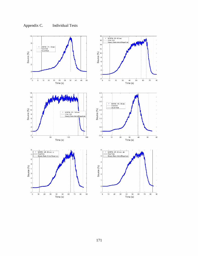
171
Appendix C. Individual Tests

172

173

174

175
Appendix D. Finite-Duration Releases grouped by Distance

176
Appendix E. Finite-Duration Releases grouped by Release Duration

177
References
1 Boybeyi, Zafer, Sethu Raman, and Paolo Zannetti. "Numerical investigation of possible role of
local meteorology in Bhopal gas accident." Atmospheric Environment 29.4 (1995): 479-496.
2 Høiset, S., et al. "Flixborough revisited—an explosion simulation approach." Journal of
hazardous materials 77.1 (2000): 1-9.
3 De Marchi, Bruna, Silvio Funtowicz, and Jerome Ravetz. "Seveso: A paradoxical classic
disaster." The long road to recovery: Community responses to industrial disaster (1996): 86-120.
4 Sheesley, D. et al. 1998. Chemical Dispersion Modeling Project, 1995 Kit Fox Field
Demonstration DOE Nevada Hazardous Spill Center. Volume I – Experiment Description and
Data Processing.
5 King, S. Bruce. 1999. The Kit Fox Field Demonstration Project and Data Set. International
Conference and Workshop on Modeling the Consequences of Accidental Releases of Hazardous
Materials.
6 Parker, Roger J. “The Flixborough Disaster. Report of the Court of Inquiry.” Department of
Employment. Her Majesty’s Stationary Office, London (1975).
7 Zhang, Wei, et al. "Effects of wall suction/blowing on two-dimensional flow past a confined
square cylinder." SpringerPlus 5.1 (2016): 985.
8 Hanna, S.R., and Chang, J.C., “Analysis of dispersion of finite-duration releases of dense gases
and recommended revisions to HEGADAS, Earth Tech Report 1411, 196 Baker Ave, Concord,
MA01742, 196 Baker Ave, Concord, MA01742, prepared for Exxon Research and Engineering,
180 Park Ave, Florham Park, NJ07932 (1995)
9 Petersen, R.L., Wind tunnel and HEGADAS simulations of finite duration releases for a specific
refinery with uniform roughness, CPP Report 91-9782, 1992
10 Taylor, Geoffrey. "Dispersion of soluble matter in solvent flowing slowly through a
tube." Proceedings of the Royal Society of London A: Mathematical, Physical and Engineering
Sciences. Vol. 219. No. 1137. The Royal Society, 1953.
11 Csanady, G. T. "Diffusion in an Ekman layer." Journal of the Atmospheric Sciences 26.3 (1969):
414-426.
12 Saffman, P. G. "The effect of wind shear on horizontal spread from an instantaneous ground
source." Quarterly Journal of the Royal Meteorological Society 88.378 (1962): 382-393.
13 Batchelor, G. K. "Diffusion from sources in a turbulent boundary layer." Arch. Mech. Stosow 3.6
(1964): 661-670.

178
14 Chatwin, P. C. "The dispersion of a puff of passive contaminant in the constant stress
region." Quarterly Journal of the Royal Meteorological Society 94.401 (1968): 350-360.
15 Wilson, D. J. "Along-wind diffusion of source transients." Atmospheric Environment
(1967) 15.4 (1981): 489-495.
16 Smith, F. B. "The role of wind shear in horizontal diffusion of ambient particles." Quarterly
Journal of the Royal Meteorological Society 91.389 (1965): 318-329.
17 Ermak. D. L., “Unpublished notes on downwind spreading formulation in finite-duration release
version of SLAB”, Lawrence Livermore National Laboratory, California (1986).
18 McMullen, Robert W. "The change of concentration standard deviations with distance." Journal
of the Air Pollution Control Association 25.10 (1975): 1057-1058.
19 Van Ulden, A. P. "A surface-layer similarity model for the dispersion of a skewed passive puff
near the ground." Atmospheric Environment. Part A. General Topics 26.4 (1992): 681-692.
20 Hanna, Steven R., and Pasquale Franzese. "Alongwind Dispersion-A Simple Similarity Formula
Compared with Observations at 11 Field Sites and in One Wind Tunnel." Journal of Applied
Meteorology 39.10 (2000): 1700-1714.
21 Drivas, Peter J., and Fredrick H. Shair. "Dispersion of an instantaneous cross-wind line source
of tracer released from an urban highway." Atmospheric Environment (1967) 8.5 (1974): 475-485.
22 Draxler, R. R. "Some observations of the along-wind dispersion parameter." Symposium on
Turbulence, Diffusion, and Air Pollution, 4th, Reno, Nev, Preprints, Research supported by the U.
S. Department of Energy. Vol. 15. No. 18. 1979.
23 Smith, F. B., and J. S. Hay. "The expansion of clusters of particles in the atmosphere." Quarterly
Journal of the Royal Meteorological Society 87.371 (1961): 82-101.
24 Sato, J., 1995: An analytical study on longitudinal diffusion in the atmospheric boundary layer.
Geophys. Mag. Ser. 2,1, 105–15
25 Robins, A. G., and J. E. Fackrell. "An experimental study of the dispersion of short duration
emissions in a turbulent boundary layer." WIT Transactions on Ecology and the Environment 28
(1970).
26 Biltoft, C., Phase I of DSWA transport and dispersion model validation study. DPG-FR-97-058,
(1997): 156.
27 Biltoft, C., Dipole Pride 26: Phase II of DSWA transport and dispersion model validation study.
DPG-FR-98-001, (1998): 130.

179
28 Watson, T. B, R. E. Keislar, B. Reese, D. H. George, and C. A. Biltoft, The DSWA Dipole Pride
26 field experiment. NOAA Tech. Memo. ERL ARL-225, (1998): 99.
29 King, S. Bruce. The Kit Fox Field Demonstration Project and Data Set. International
Conference and Workshop on Modeling the Consequences of Accidental Releases of Hazardous
Materials. (1999).
30 Spicer, T. and Havens, J. Description and Analysis of Atmospheric Dispersion Tests Conducted
by EPA. International Conference and Workshop on Modeling the Consequences of Accidental
Releases of Hazardous Materials. (1999).
31 Sheesley, D. et al.. Chemical Dispersion Modeling Project, 1995 Kit Fox Field Demonstration
DOE Nevada Hazardous Spill Center. Volume I – Experiment Description and Data Processing.
(1998).
32 Hanna, S. R., and K. W. Steinberg, Studies of dense gas dispersion from short-duration transient
releases over rough surfaces during stable conditions. Air Pollution Modeling and Its Applications
XI,Plenum Press, (1996): 481–490.
33 Nickola, P. W., J. D. Ludwick, and J. V. Ramsdell Jr., An inert gas tracer system for monitoring
the real-time history of a diffusing plume or puff. J. Appl. Meteor.,9, (1970): 621–626.
34 Bowers, J. F., G. E. Start, R. G. Carter, T. B. Watson, K. L. Clawson, and T. L. Crawford,
Experimental design and results for the Long-Range Overwater Diffusion (LROD) Experiment.
DPG/JCP-94/012, (1994): 531.
35 Biltoft, C., S. D. Turley, T. B. Watson, G. H. Crescenti, and R. G. Carter, Over-Land
Atmospheric Dispersion (OLAD) test summary and analysis. WDTC Doc. WDTC/JCP-99/048,
(1999): 38.
36 Smith, and B. L. Niemann, Shoreline diffusion program, Oceanside, CA. Vols. I and II. MRI-
64-FR-860, (1969): 230 and 456.
37 Hilst, G. R., and N. E. Bowne, A study of the diffusion of aerosols released from aerial line
sources upwind of an urban complex. Vols. I and II. Rep. DA-42-007-AMC-38®, (1966): 231 and
583.
38 Sato, J., F. Kimura, and T. Yoshikawa, The longitudinal spread of puff in the short range
diffusion experiment. Pap. Meteor. Geophys.,32, (1981): 155–162.
39 Golder, Donald. "Relations among stability parameters in the surface layer." Boundary-Layer
Meteorology 3.1 (1972): 47-58.
40 Davis, Richard A. “Practical Numerical Methods for Chemical Engineers: Using Excel with
VBA”. Lexington, KY, (2015).

180
41 Draper, Norman Richard, Harry Smith, and Elizabeth Pownell. Applied regression analysis. Vol.
3. New York: Wiley, (1966).
42 Conover, William Jay, and William Jay Conover. "Practical nonparametric statistics." (1980).
43 Hanna, S. R., J. C. Chang, and D. G. Strimaitis. "Hazardous gas model evaluation with field
observations." Atmospheric Environment. Part A. General Topics 27.15 (1993): 2265-2285. 44 DNV GL. DNV GL Theory Manual for Unified Dispersion Model. London UK 2015.
45 Wilson, David J. Concentration fluctuations and averaging time in vapor clouds. John Wiley &
Sons, 2010.
46 Havens, J., and T. Spicer. "Vapor dispersion and thermal hazard modelling." Final topical
report to Gas Technology Institute under sub-contract K 100029184 (2006).
47 Walker, H., and J. Havens. “Comparison of hot wire and laser Doppler anemometry
measurements of the turbulence structure of an ultra low speed wind tunnel boundary layer.” Data
report, Chemical Hazards Research Center, University of Arkansas, Fayetteville, AR 72701
(1998).
48 Irwin, H. P. A. H. "The design of spires for wind simulation." Journal of Wind Engineering and
Industrial Aerodynamics7.3 (1981): 361-366.
49 Cambustion. “Fast FID Principles.” Exhaust Gas Recirculation (EGR), NOx and Particulate
Measurement | Cambustion, 2018, www.cambustion.com/products/hfr500/fast-fid-principles.
50 GadgetReview. “ An illustration of a VOC meter detecting pollutants in the surrounding air”
How do VOC Meters Work? | GadgetReview, 2018, http://www.gadgetreview.com/what-is-voc-
Meter
51 Koflo. “KD-981” Koflo, 2018, https://www.koflo.com/drawings/pdf/kd-981.pdf
52 “Weber Number” Engineering Toolbox, 2018, https://www.engineeringtoolbox.com/weber-
number-d_583.html
53 Havens, Jerry, Heather Walker, and Thomas O. Spicer. "Wind tunnel study of air entrainment
into two-dimensional dense gas plumes at the Chemical Hazards Research Center." Atmospheric
Environment 35.13 (2001): 2305-2317.
54 Wieslander, Gunillla, D. Norback, and Torsten Lindgren. “Experimental exposure to propylene
glycol mist in aviation emergency training: acute oculat and respiratory effects.” Occupational
and Environmental Medicine 58.19 (2001): 649-655.
55 TSI. (2005). Phase Doppler Particle Analyzer (PDPA) / Laser Dopppler Velocimeter (LDV)
Operations Manual. Shoreview, MN.

181
56 Mathieu J., Scott J., 2000. An Introduction to Turbulent Flow. Cambridge University
Press, Cambridge, UK.
57 C. G. Lomas, Fundamentals of Hot Wire Anemometry. Cambridge University Press, 2011.
58 “Measurement Techniques for Instantaneous Velocity”, Emaze – amazing presentations.
[Online]. Available: https://www.emaze.com/@ALORRLQI/TP-PRESENTATiON
59 Stull, B. R., 1988. An Introduction to Boundary Layer Meterology. Boston: Kluwer Academic
Publishers.
60 C. V. Mashuga and D. A. Crowl, “Application of the Flammability Diagram for Evaluation of
Fire and Explosion Hazards of Flammable Vapors,” Process Safety Progress (1998), 17(3): 176.
61 Wilson, David J. Concentration fluctuations and averaging time in vapor clouds. John Wiley &
Sons, 2010. Pg 42.
62 Hall, D. J., et al. “The Effect of Release Time on the Dispersion of a Fixed Inventory of Heavy
Gas – A Wind Tunnel Model Study.” Physmod 2007.
63 Hall, D., R. Waters, and G. Marsland, Repeat variability in instantaneously release heavy gas
clouds – some wind tunnel model experiments. 1991.
64 Wilson, David J. Concentration fluctuations and averaging time in vapor clouds. John Wiley &
Sons, 2010. Pg 43.
65 Hanna, Steven R., and Joseph C. Chang. “Use of the Kit Fox field data to analyze dense gas
dispersion modeling dispersion modeling issues.” Atmospheric Environment. 35.13 (2001): 2231-
2242.
66 Hanna, S.R., Chang, J.C., 1995. Analysis of dispersion of finite duration releases of dense gases
and recommended revisions to HEGADAS. Earth Tech. Report No. 1411, prepared for Exxon
Research and Engineering, 180 Park Ave., Florham Park, NJ 07932.