Experiments on the Flow Field and Acoustic Properties of a

Flow Turbulence Combust (2009) 83:587–611DOI 10.1007/s10494-009-9212-4

Experiments on the Flow Field and AcousticProperties of a Mach number 0·75 TurbulentAir Jet at a Low Reynolds Number

Harmen J. Slot · Peter Moore · René Delfos ·Bendiks Jan Boersma

Received: 30 October 2007 / Accepted: 18 March 2009 / Published online: 17 April 2009© The Author(s) 2009. This article is published with open access at Springerlink.com

Abstract In this paper we present the experimental results of a detailed investigationof the flow and acoustic properties of a turbulent jet with Mach number 0·75 andReynolds number 3·5 103. We describe the methods and experimental proceduresfollowed during the measurements, and subsequently present the flow field andacoustic field. The experiment presented here is designed to provide accurate andreliable data for validation of Direct Numerical Simulations of the same flow. MeanMach number surveys provide detailed information on the centreline mean Machnumber distribution, radial development of the mean Mach number and the evolu-tion of the jet mixing layer thickness both downstream and in the early stages of jetdevelopment. Exit conditions are documented by measuring the mean Mach numberprofile immediately above the nozzle exit. The fluctuating flow field is characterisedby means of a hot-wire, which produced radial profiles of axial turbulence at severalstations along the jet axis and the development of flow fluctuations through the jetmixing layer. The axial growth rate of the jet instabilities are determined as functionof Strouhal number, and the axial development of several spectral components isdocumented. The directivity of the overall sound pressure level and several spectralcomponents were investigated. The spectral content of the acoustic far field is shownto be compatible with findings of hot-wire experiments in the mixing layer of the jet.In addition, the measured acoustic spectra agree with Tam’s large-scale similarityand fine-scale similarity spectra (Tam et al., AIAA Pap 96, 1996).

Keywords Jet noise · Jet flow · Low Reynolds number flow · Validation · Simulation

H. J. Slot (B) · P. Moore · R. Delfos · B. J. BoersmaLaboratory for Aero and Hydrodynamics, Delft University of Technology,Leeghwaterstraat 21, 2628 CA Delft, The Netherlandse-mail: [email protected]

588 Flow Turbulence Combust (2009) 83:587–611

1 Introduction

Inherent to computing limitations, a Direct Numerical Simulation (DNS) of acompressible jet flow is commonly performed on high Mach number jets with a lowReynolds number such as the DNS of Freund [10] and Moore et al. [21]. Before jetflow or jet noise predictions based on a DNS of a turbulent flow can be relied upon,the numerical work need be carefully validated by means of detailed and reliableexperimental evidence. The validation would require detailed information of boththe flow field and the acoustic far field. There is little experimental data availablethat would facilitate such a validation of turbulent jets with a high Mach number andlow Reynolds number. The documented experimental work on subsonic jets concernmeasurements focusing either on properties of the flow field or on properties of theacoustic far field. Turbulence characteristics of subsonic turbulent jets with a moder-ate to high Reynolds number (Re ≈ 103−105) were reported by Panchapakesan &Lumley [24], Hussein et al. [12], Zaman [40], Wygnanski & Fiedler [38], Laufer andYen [15] and Bradshaw et al. [7]. Most of the work mentioned concerned low velocityjets (Ma<0·3), and do not or briefly discuss properties of the acoustic far field.Contrary to the aforementioned, Mollo-Christensen et al. [20], Lush [16], Tanna [34]and Ahuja [1] reported properties of the acoustic far field of subsonic turbulentjets in detail, but did not investigate the flow field. Stromberg et al. [29] combinedmeasurements of the acoustic far field and flow field of a subsonic turbulent jet witha low Reynolds number in their work, but used their experimental results mainly toilluminate the process of jet noise production. In addition, little information of thefluctuating flow field was reported. The experimental work reported on in this paperaims to provide accurate and reliable data that can be used for the validation of aDirect Numerical Simulation of a turbulent jet with a Mach number (Ma=U/c) 0·75and Reynolds number (Re= ρUd/μ) 3.5 ·103, where ρ denotes density (kg/m3), U isthe jet flow velocity (m/s), c denotes sound velocity (m/s), nozzle diameter d= 8·10−3

(m) and μ denotes dynamic viscosity (Pa·s).Over the range of Reynolds number considered in a DNS, the effects of Reynolds

number have been shown to be important [5, 9]. Study of the jet noise producingmechanisms is relatively less complex with low Reynolds number jets as the rangeof turbulence scales present in the flow is fairly limited compared to high Reynoldsnumber jets. Consequently, the jet noise producing mechanisms are thought to bemore transparent in jets with low Reynolds numbers.

This paper is organised as follows. First, a description of the experimental setupand procedures is given in Section 2. Section 2.1 describes the pressure chamberand the jet exit nozzle in detail. Details concerning the flow field and acousticmeasurement techniques and calibration procedures are described in Sections 2.2and 2.3.

The results are presented in Section 3, and are split into results concerning theflow field (3.1) and the acoustic far field (3.2). Mean flow properties are presented inSection 3.1.1, and concern jet exit conditions, mean Mach number profiles and thedevelopment of the jet mixing layer. Fluctuating flow field properties are detailed inSection 3.1.2. The spectral content of density fluctuations in the jet mixing layer aredocumented, and allow an inspection of the development of the fundamental and thesubharmonic mode throughout the jet mixing layer. Spatial linear instability theoryis used to asses the axial growth rates as function of Strouhal number.

Flow Turbulence Combust (2009) 83:587–611 589

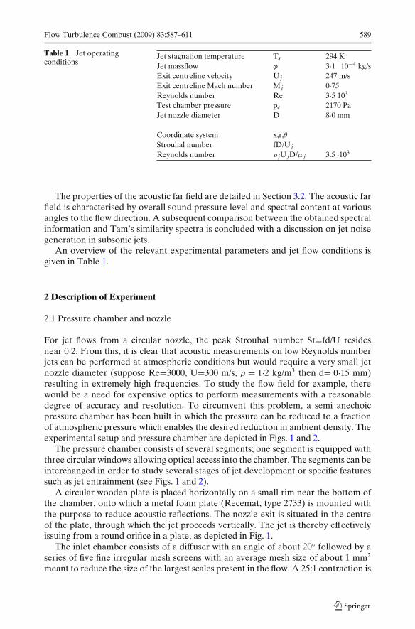
Table 1 Jet operatingconditions

Jet stagnation temperature Ts 294 KJet massflow φ 3·1 10−4 kg/sExit centreline velocity U j 247 m/sExit centreline Mach number M j 0·75Reynolds number Re 3·5 103

Test chamber pressure pc 2170 PaJet nozzle diameter D 8·0 mm

Coordinate system x,r,θStrouhal number fD/U j

Reynolds number ρ jU jD/μ j 3.5 ·103

The properties of the acoustic far field are detailed in Section 3.2. The acoustic farfield is characterised by overall sound pressure level and spectral content at variousangles to the flow direction. A subsequent comparison between the obtained spectralinformation and Tam’s similarity spectra is concluded with a discussion on jet noisegeneration in subsonic jets.

An overview of the relevant experimental parameters and jet flow conditions isgiven in Table 1.

2 Description of Experiment

2.1 Pressure chamber and nozzle

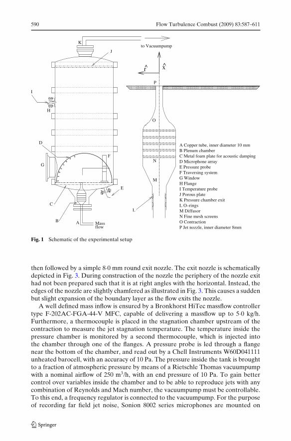
For jet flows from a circular nozzle, the peak Strouhal number St=fd/U residesnear 0·2. From this, it is clear that acoustic measurements on low Reynolds numberjets can be performed at atmospheric conditions but would require a very small jetnozzle diameter (suppose Re=3000, U=300 m/s, ρ = 1·2 kg/m3 then d= 0·15 mm)resulting in extremely high frequencies. To study the flow field for example, therewould be a need for expensive optics to perform measurements with a reasonabledegree of accuracy and resolution. To circumvent this problem, a semi anechoicpressure chamber has been built in which the pressure can be reduced to a fractionof atmospheric pressure which enables the desired reduction in ambient density. Theexperimental setup and pressure chamber are depicted in Figs. 1 and 2.

The pressure chamber consists of several segments; one segment is equipped withthree circular windows allowing optical access into the chamber. The segments can beinterchanged in order to study several stages of jet development or specific featuressuch as jet entrainment (see Figs. 1 and 2).

A circular wooden plate is placed horizontally on a small rim near the bottom ofthe chamber, onto which a metal foam plate (Recemat, type 2733) is mounted withthe purpose to reduce acoustic reflections. The nozzle exit is situated in the centreof the plate, through which the jet proceeds vertically. The jet is thereby effectivelyissuing from a round orifice in a plate, as depicted in Fig. 1.

The inlet chamber consists of a diffuser with an angle of about 20◦ followed by aseries of five fine irregular mesh screens with an average mesh size of about 1 mm2

meant to reduce the size of the largest scales present in the flow. A 25:1 contraction is


to Vacuumpump

Massflow

x̂r̂

AB

C

D

E

F

G

H

I

J

K

L

O

N

M

A Copper tube, inner diameter 10 mmB Plenum chamber

D Microphone arrayE Pressure probeF Traversing systemG WindowH FlangeI Temperature probeJ Porous plateK Pressure chamber exitL O–ringsM DiffusorN Fine mesh screensO Contraction

C Metal foam plate for acoustic damping

P

P Jet nozzle, inner diameter 8mm

Fig. 1 Schematic of the experimental setup

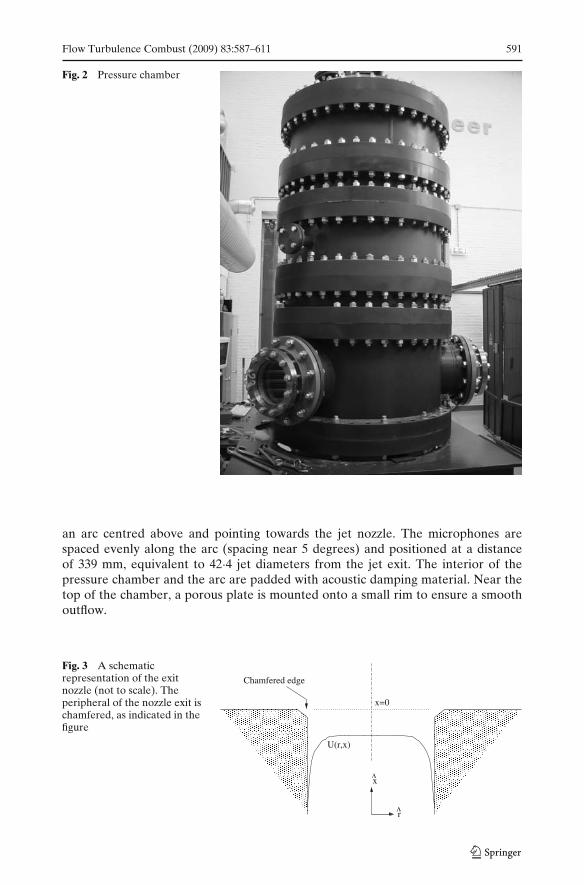
then followed by a simple 8·0 mm round exit nozzle. The exit nozzle is schematicallydepicted in Fig. 3. During construction of the nozzle the periphery of the nozzle exithad not been prepared such that it is at right angles with the horizontal. Instead, theedges of the nozzle are slightly chamfered as illustrated in Fig. 3. This causes a suddenbut slight expansion of the boundary layer as the flow exits the nozzle.

A well defined mass inflow is ensured by a Bronkhorst HiTec massflow controllertype F-202AC-FGA-44-V MFC, capable of delivering a massflow up to 5·0 kg/h.Furthermore, a thermocouple is placed in the stagnation chamber upstream of thecontraction to measure the jet stagnation temperature. The temperature inside thepressure chamber is monitored by a second thermocouple, which is injected intothe chamber through one of the flanges. A pressure probe is led through a flangenear the bottom of the chamber, and read out by a Chell Instruments W60D041111unheated barocell, with an accuracy of 10 Pa. The pressure inside the tank is broughtto a fraction of atmospheric pressure by means of a Rietschle Thomas vacuumpumpwith a nominal airflow of 250 m3/h, with an end pressure of 10 Pa. To gain bettercontrol over variables inside the chamber and to be able to reproduce jets with anycombination of Reynolds and Mach number, the vacuumpump must be controllable.To this end, a frequency regulator is connected to the vacuumpump. For the purposeof recording far field jet noise, Sonion 8002 series microphones are mounted on


Fig. 2 Pressure chamber

an arc centred above and pointing towards the jet nozzle. The microphones arespaced evenly along the arc (spacing near 5 degrees) and positioned at a distanceof 339 mm, equivalent to 42·4 jet diameters from the jet exit. The interior of thepressure chamber and the arc are padded with acoustic damping material. Near thetop of the chamber, a porous plate is mounted onto a small rim to ensure a smoothoutflow.

Fig. 3 A schematicrepresentation of the exitnozzle (not to scale). Theperipheral of the nozzle exit ischamfered, as indicated in thefigure

Chamfered edge

x

v

v

r

U(r,x)

x=0


2.2 Flow field measurements

The flow field fluctuations were investigated by means of a hot-wire. The hot-wiredata reduction method we follow is a combination of the work of Ko et al. [13] andMorkovin [22]. Ko et al. recognised the potential of their data reduction method byexplicitly accounting for the energy transfer to the hot-wire that is returned as end-loss to the hot-wire supports, circumventing the need to define a modified Nusseltnumber.

After a first series of measurements, the hot-wire bridge voltage fluctuationswere found to be approximately proportional to density fluctuations. Normalisedfluctuations T′

rms/T and u′rms/u were found to contribute about 5% or less to the

output and will not be taken into account here in after. The raw hot-wire signalwas filtered by a Butterworth low-pass filter with a cut-off frequency of 25 kHz toeliminate electronic resonances and thereafter sampled at 500 kHz. Details on thefollowed hot-wire calibration procedure can be found in Appendix A.

A conventional Prandtl tube with an outer diameter of 1·0 mm was used in allmean velocity surveys, except for the measurement of the mean velocity profileimmediately downstream of the nozzle exit plane where significant spatial resolutionin the jet shear layer is required (Fig. 8a). For this particular investigation theconventional tube was replaced with a glass Prandtl tube with an outer diameterof 100 μm. A differential pressure sensor sensitive up to a pressure differenceequivalent to a 140 mm water column was ported to the Prandtl tube and to a secondtube, positioned well away from the flow, which measured static pressure. A twodimensional traversing system was used to traverse the Prandtl tube in the spanwiseand flow direction.

2.3 Acoustic far field measurements

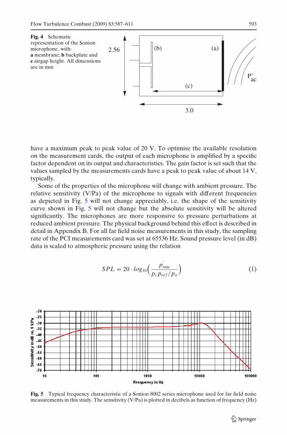
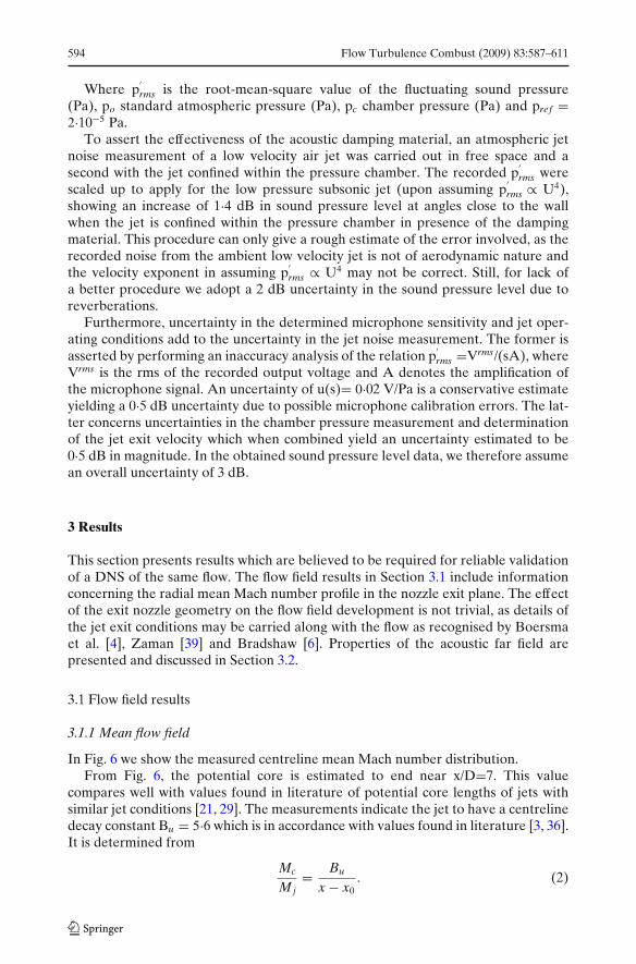
Acoustic far field measurements are performed using Sonion 8002 series micro-phones. Assuming that U=300 m/s and St=0·2, we may expect the dominant portionof the noise radiated from a subsonic jet given a 8·0 mm exit nozzle to havefrequencies around approximately StU/d ≈ 8 kHz. The microphones are sensitive upto frequencies near 20 kHz, and may therefore be regarded as suitable for perform-ing aeroacoustic measurements on this particular flow. These Sonion microphonesare simple electret microphones as shown in Fig. 4. A representative frequencyresponse of the microphone is shown in Fig. 5. The microphones are quite smallin size; with their cross sectional diameter of 3·0 mm (≈1/10”), their characteristicdimension is much smaller than the wavelengths of the jet noise propagating tofar field. The 8002 series Sonion microphones are not designed to be used foraeroacoustic measurements, and consequently are not calibrated separately by themanufacturer. They come accompanied with specifications that are representativefor the entire series. Consequently, each microphone is calibrated separately bymeans of a pistonphone. For this purpose we use a Grass 240A pistonphone whichproduces pressure perturbations at a frequency of 250 Hz with a sound pressure levelof 113·99 dB at atmospheric conditions. The microphone output signals are read intoa computer by two National Instruments PCI 4472 measurements cards. They areequipped with eight input channels and are capable of simultaneously sampling 8channels at 102 kHz. The specifications further indicate that the input is allowed to


Fig. 4 Schematicrepresentation of the Sonionmicrophone, with:a membrane; b backplate andc airgap height. All dimensionsare in mm

P’ac

(b) (a)

(c)

2.56

3.0

have a maximum peak to peak value of 20 V. To optimise the available resolutionon the measurement cards, the output of each microphone is amplified by a specificfactor dependent on its output and characteristics. The gain factor is set such that thevalues sampled by the measurements cards have a peak to peak value of about 14 V,typically.

Some of the properties of the microphone will change with ambient pressure. Therelative sensitivity (V/Pa) of the microphone to signals with different frequenciesas depicted in Fig. 5 will not change appreciably, i.e. the shape of the sensitivitycurve shown in Fig. 5 will not change but the absolute sensitivity will be alteredsignificantly. The microphones are more responsive to pressure perturbations atreduced ambient pressure. The physical background behind this effect is described indetail in Appendix B. For all far field noise measurements in this study, the samplingrate of the PCI measurements card was set at 65536 Hz. Sound pressure level (in dB)data is scaled to atmospheric pressure using the relation

SPL = 20 · log10

( p′rms

pc pref /po

)(1)

Fig. 5 Typical frequency characteristic of a Sonion 8002 series microphone used for far field noisemeasurements in this study. The sensitivity (V/Pa) is plotted in decibels as function of frequency (Hz)


Where p′rms is the root-mean-square value of the fluctuating sound pressure

(Pa), po standard atmospheric pressure (Pa), pc chamber pressure (Pa) and pref =2·10−5 Pa.

To assert the effectiveness of the acoustic damping material, an atmospheric jetnoise measurement of a low velocity air jet was carried out in free space and asecond with the jet confined within the pressure chamber. The recorded p

′rms were

scaled up to apply for the low pressure subsonic jet (upon assuming p′rms ∝ U4),

showing an increase of 1·4 dB in sound pressure level at angles close to the wallwhen the jet is confined within the pressure chamber in presence of the dampingmaterial. This procedure can only give a rough estimate of the error involved, as therecorded noise from the ambient low velocity jet is not of aerodynamic nature andthe velocity exponent in assuming p

′rms ∝ U4 may not be correct. Still, for lack of

a better procedure we adopt a 2 dB uncertainty in the sound pressure level due toreverberations.

Furthermore, uncertainty in the determined microphone sensitivity and jet oper-ating conditions add to the uncertainty in the jet noise measurement. The former isasserted by performing an inaccuracy analysis of the relation p

′rms =Vrms/(sA), where

Vrms is the rms of the recorded output voltage and A denotes the amplification ofthe microphone signal. An uncertainty of u(s)= 0·02 V/Pa is a conservative estimateyielding a 0·5 dB uncertainty due to possible microphone calibration errors. The lat-ter concerns uncertainties in the chamber pressure measurement and determinationof the jet exit velocity which when combined yield an uncertainty estimated to be0·5 dB in magnitude. In the obtained sound pressure level data, we therefore assumean overall uncertainty of 3 dB.

3 Results

This section presents results which are believed to be required for reliable validationof a DNS of the same flow. The flow field results in Section 3.1 include informationconcerning the radial mean Mach number profile in the nozzle exit plane. The effectof the exit nozzle geometry on the flow field development is not trivial, as details ofthe jet exit conditions may be carried along with the flow as recognised by Boersmaet al. [4], Zaman [39] and Bradshaw [6]. Properties of the acoustic far field arepresented and discussed in Section 3.2.

3.1 Flow field results

3.1.1 Mean flow field

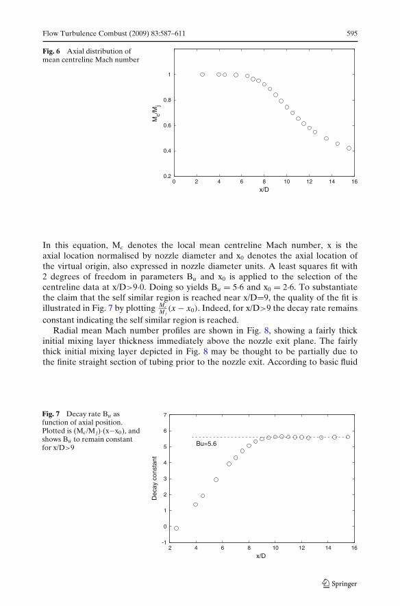
In Fig. 6 we show the measured centreline mean Mach number distribution.From Fig. 6, the potential core is estimated to end near x/D=7. This value

compares well with values found in literature of potential core lengths of jets withsimilar jet conditions [21, 29]. The measurements indicate the jet to have a centrelinedecay constant Bu = 5·6 which is in accordance with values found in literature [3, 36].It is determined from

Mc

Mj= Bu

x − x0. (2)


Fig. 6 Axial distribution ofmean centreline Mach number

0.2

0.4

0.6

0.8

1

0 2 4 6 8 10 12 14 16

Mc/M

j

x/D

In this equation, Mc denotes the local mean centreline Mach number, x is theaxial location normalised by nozzle diameter and x0 denotes the axial location ofthe virtual origin, also expressed in nozzle diameter units. A least squares fit with2 degrees of freedom in parameters Bu and x0 is applied to the selection of thecentreline data at x/D>9·0. Doing so yields Bu = 5·6 and x0 = 2·6. To substantiatethe claim that the self similar region is reached near x/D=9, the quality of the fit isillustrated in Fig. 7 by plotting Mc

Mj(x − x0). Indeed, for x/D>9 the decay rate remains

constant indicating the self similar region is reached.Radial mean Mach number profiles are shown in Fig. 8, showing a fairly thick

initial mixing layer thickness immediately above the nozzle exit plane. The fairlythick initial mixing layer depicted in Fig. 8 may be thought to be partially due tothe finite straight section of tubing prior to the nozzle exit. According to basic fluid

Fig. 7 Decay rate Bu asfunction of axial position.Plotted is (Mc/M j)·(x−x0), andshows Bu to remain constantfor x/D>9

-1

0

1

2

3

4

5

6

7

2 4 6 8 10 12 14 16

Dec

ay c

onst

ant

x/D

Bu=5.6


0

0.5

1.0

Nor

mal

ised

Mac

h nu

mbe

r M

/Mj

(a)

0.5

1.0 (b)

0

0.5

1.0

0 0.2 0.4 0.6 0.8

(c)

r/D

0.5

1.0

0 0.2 0.4 0.6 0.8 1.0

(d)

Fig. 8 Radial mean Mach number profile immediately above nozzle exit plane (a); and at axiallocations x/D: b 2·5; c 5 and d 10

mechanics [2] the thickness of a boundary layer after length x along a horizontal platemay be determined from

δ = 5L√Rex

, (3)

in which the Reynolds number is based on length x of the straight section of thenozzle. Based on the above equation, we can estimate the exit mixing layer thicknessto be δ/2D= 0·1 which is in excellent agreement with the experimentally obtainedvalue of δ/2D= 0·11 (see Fig. 11). As mentioned before in Section 2.1, the chamferededge of the nozzle also contributes to the fairly thick mixing layer at the nozzle exit.

To assert whether the mixing layer immediately above the nozzle exit is laminar, aBlasius profile is superimposed onto the radial mean Mach number data obtained atx/D=0 as depicted in Fig. 9. The figure shows the radial Mach number profile of theinitial mixing layer to be in accordance with the Blasius profile, indicating the initialmixing layer is indeed laminar.

A closer examination of the radial mean velocity distributions reveals that allprofiles collapse onto a common curve as shown in Fig. 10, in which a curve fit isused similar to the one used by Laufer et al. [14] for subsonic jets. This curve fit takesthe form

M(η) ={

exp[−2 · 773(η + 0 · 5)2] for η ≥ −0 · 51 for η ≤ −0 · 5


Fig. 9 Confirmation that themixing layer at x/D=0 islaminar: circles, Radial meanMach number profile; line,Blasius profile

0

0.2

0.4

0.6

0.8

1.0

0 0.1 0.2 0.3 0.4 0.5

M/M

j

Radial position (r/D)

In this equation, the self similarity coordinate η =[r−r(0·5)]/δ in which r(0·5) denotesthe radial location at which the local Mach number is exactly 0·5 times the centrelinevalue at that particular axial coordinate.

Let us examine the development of the jet mixing layer more closely. The growthof the jet mixing layer thickness and jet half-radii as fraction of the jet diameterare considered in detail in Fig. 11. Following Troutt & McLaughlin [35], the mixinglayer thicknesses δ were calculated from radial mean Mach number profiles uponassuming that δ =r(0·1)−r(0·99). In Fig. 8 the mixing layer thickness displays amoderate growth in the early development stages, as shown in Fig. 11. Shortly beforethe end of the potential core is reached, the mixing layer thickness displays a rapidradial expansion. We may therefore conclude that transition from a laminar to aturbulent mixing layer occurs between 5 to 6 jet diameters downstream, after whichthe growth rate of the mixing layer thickness is significantly increased. After the endof the potential core, the mixing layer thickness grows approximately linear with axialdistance.

Fig. 10 Radial mean Machnumber profiles plottedagainst self similaritycoordinate η at axial locationsx/D: circles, 2·5; upsidedowntriangles, 5; right-side-uptriangles, 10

0

0.2

0.4

0.6

0.8

1

-0.8 -0.6 -0.4 -0.2 0 0.2 0.4 0.6 0.8

M(η

)/M

c(x)

η=(r-r(0.5))/δ


Fig. 11 Jet mixing layerdevelopment, characterised bymixing layer thickness δ/2D:circles and jet half radiir(0·5)/D: squares

0

0.2

0.4

0.6

0.8

1

1.2

0 2 4 6 8 10 12 14

r(0

.5)/

D -

-δ/

2D

x/D

3.1.2 Fluctuating flow field

Density fluctuations as fraction of local density are shown in Fig. 12. During the firstcouple of jet diameters downstream of the nozzle exit the density fluctuations growapproximately exponentially with distance within the jet mixing layer, as fraction ofthe local density. The density fluctuations as fraction of local mean density saturatein amplitude near x/D= 3·5, and remain in the same order of magnitude until x/D=6after which a gradual decay is set in. The decay is most likely linked with the effectsof jet spreading, which becomes significant once the potential core has collapsed nearx/D=7.

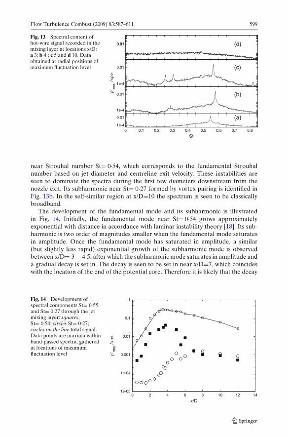
The density fluctuations in the mixing layer find significant contributions fromfluctuations with specific frequencies, as illustrated in the hot-wire spectra shownin Fig. 13. The hot-wire spectra are based on 16384 point Fourier transforms on400 windows yielding an averaged spectrum with a 30·5 Hz spectral resolution.From the figure it becomes apparent that the fluctuations in the jet mixing layerare initially dominated by instabilities centred around a relatively discrete frequency

Fig. 12 Density fluctuationsas fraction of local meandensity at several probelocations in the shear layer.Data was gathered at theradial location of maximumfluctuation level

0.001

0.01

0.1

1

0 2 4 6 8 10 12 14

x/D

ρ’

/<

ρ>rm

s


Fig. 13 Spectral content ofhot-wire signal recorded in themixing layer at locations x/D:a 3; b 4·; c 5 and d 10. Dataobtained at radial positions ofmaximum fluctuation level

1e-4

0.01

0 0.1 0.2 0.3 0.4 0.5 0.6 0.7 0.8

St

(a)1e-4

0.01 (b)

1e-4

0.01

ρ’

/<

ρ>

(c)

0.010.01 (d)

rms

near Strouhal number St= 0·54, which corresponds to the fundamental Strouhalnumber based on jet diameter and centreline exit velocity. These instabilities areseen to dominate the spectra during the first few diameters downstream from thenozzle exit. Its subharmonic near St= 0·27 formed by vortex pairing is identified inFig. 13b. In the self-similar region at x/D=10 the spectrum is seen to be classicallybroadband.

The development of the fundamental mode and its subharmonic is illustratedin Fig. 14. Initially, the fundamental mode near St= 0·54 grows approximatelyexponential with distance in accordance with laminar instability theory [18]. Its sub-harmonic is two order of magnitudes smaller when the fundamental mode saturatesin amplitude. Once the fundamental mode has saturated in amplitude, a similar(but slightly less rapid) exponential growth of the subharmonic mode is observedbetween x/D= 3 − 4·5, after which the subharmonic mode saturates in amplitude anda gradual decay is set in. The decay is seen to be set in near x/D=7, which coincideswith the location of the end of the potential core. Therefore it is likely that the decay

Fig. 14 Development ofspectral components St= 0·55and St= 0·27 through the jetmixing layer: squares,St= 0·54; circles St= 0·27;circles on the line total signal.Data points are maxima withinband-passed spectra, gatheredat locations of maximumfluctuation level

1e-05

1e-04

0.001

0.01

0.1

1

0 2 4 6 8 10 12 14

x/D

ρ’rm

s /<ρ>


in density fluctuations are connected to the spreading of energy over a larger radialdistance within the jet.

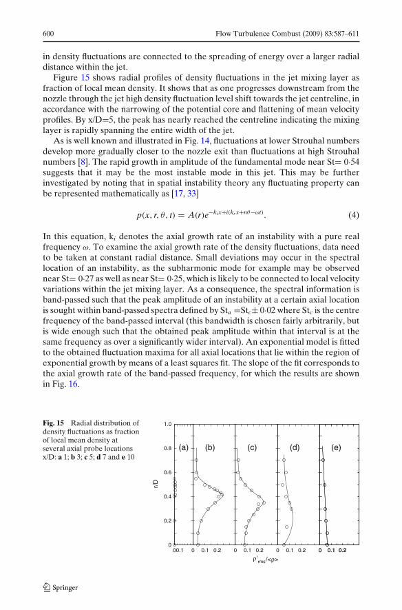
Figure 15 shows radial profiles of density fluctuations in the jet mixing layer asfraction of local mean density. It shows that as one progresses downstream from thenozzle through the jet high density fluctuation level shift towards the jet centreline, inaccordance with the narrowing of the potential core and flattening of mean velocityprofiles. By x/D=5, the peak has nearly reached the centreline indicating the mixinglayer is rapidly spanning the entire width of the jet.

As is well known and illustrated in Fig. 14, fluctuations at lower Strouhal numbersdevelop more gradually closer to the nozzle exit than fluctuations at high Strouhalnumbers [8]. The rapid growth in amplitude of the fundamental mode near St= 0·54suggests that it may be the most instable mode in this jet. This may be furtherinvestigated by noting that in spatial instability theory any fluctuating property canbe represented mathematically as [17, 33]

p(x, r, θ, t) = A(r)e−kix+i(kr x+nθ−ωt). (4)

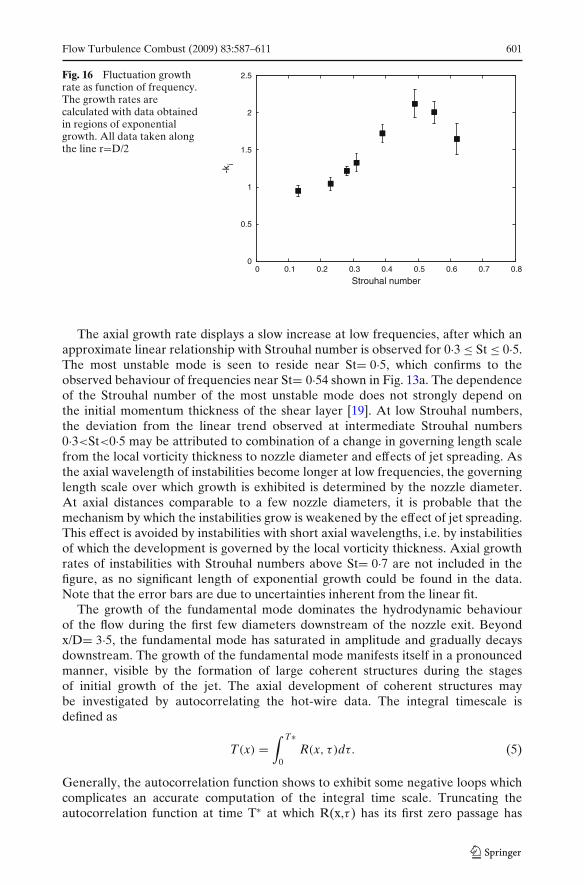
In this equation, ki denotes the axial growth rate of an instability with a pure realfrequency ω. To examine the axial growth rate of the density fluctuations, data needto be taken at constant radial distance. Small deviations may occur in the spectrallocation of an instability, as the subharmonic mode for example may be observednear St= 0·27 as well as near St= 0·25, which is likely to be connected to local velocityvariations within the jet mixing layer. As a consequence, the spectral information isband-passed such that the peak amplitude of an instability at a certain axial locationis sought within band-passed spectra defined by Sta =Stc± 0·02 where Stc is the centrefrequency of the band-passed interval (this bandwidth is chosen fairly arbitrarily, butis wide enough such that the obtained peak amplitude within that interval is at thesame frequency as over a significantly wider interval). An exponential model is fittedto the obtained fluctuation maxima for all axial locations that lie within the region ofexponential growth by means of a least squares fit. The slope of the fit corresponds tothe axial growth rate of the band-passed frequency, for which the results are shownin Fig. 16.

Fig. 15 Radial distribution ofdensity fluctuations as fractionof local mean density atseveral axial probe locationsx/D: a 1; b 3; c 5; d 7 and e 10

1.0

0.8

0.6

0.4

0.2

00.10

r/D

(a)

0.20.10

(b)

0.20.10

(c)

0.20.10

(d)

0.20.10 0.20.10

(e)


Fig. 16 Fluctuation growthrate as function of frequency.The growth rates arecalculated with data obtainedin regions of exponentialgrowth. All data taken alongthe line r=D/2

0

0.5

1

1.5

2

2.5

0 0.1 0.2 0.3 0.4 0.5 0.6 0.7 0.8

-ki

Strouhal number

The axial growth rate displays a slow increase at low frequencies, after which anapproximate linear relationship with Strouhal number is observed for 0·3 ≤ St ≤ 0·5.The most unstable mode is seen to reside near St= 0·5, which confirms to theobserved behaviour of frequencies near St= 0·54 shown in Fig. 13a. The dependenceof the Strouhal number of the most unstable mode does not strongly depend onthe initial momentum thickness of the shear layer [19]. At low Strouhal numbers,the deviation from the linear trend observed at intermediate Strouhal numbers0·3<St<0·5 may be attributed to combination of a change in governing length scalefrom the local vorticity thickness to nozzle diameter and effects of jet spreading. Asthe axial wavelength of instabilities become longer at low frequencies, the governinglength scale over which growth is exhibited is determined by the nozzle diameter.At axial distances comparable to a few nozzle diameters, it is probable that themechanism by which the instabilities grow is weakened by the effect of jet spreading.This effect is avoided by instabilities with short axial wavelengths, i.e. by instabilitiesof which the development is governed by the local vorticity thickness. Axial growthrates of instabilities with Strouhal numbers above St= 0·7 are not included in thefigure, as no significant length of exponential growth could be found in the data.Note that the error bars are due to uncertainties inherent from the linear fit.

The growth of the fundamental mode dominates the hydrodynamic behaviourof the flow during the first few diameters downstream of the nozzle exit. Beyondx/D= 3·5, the fundamental mode has saturated in amplitude and gradually decaysdownstream. The growth of the fundamental mode manifests itself in a pronouncedmanner, visible by the formation of large coherent structures during the stagesof initial growth of the jet. The axial development of coherent structures maybe investigated by autocorrelating the hot-wire data. The integral timescale isdefined as

T(x) =∫ T∗

0R(x, τ )dτ. (5)

Generally, the autocorrelation function shows to exhibit some negative loops whichcomplicates an accurate computation of the integral time scale. Truncating theautocorrelation function at time T∗ at which R(x,τ ) has its first zero passage has


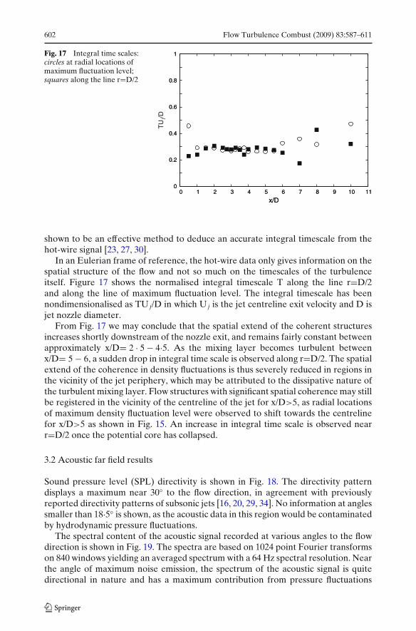
Fig. 17 Integral time scales:circles at radial locations ofmaximum fluctuation level;squares along the line r=D/2

0

0.2

0.4

0.6

0.8

1

0 1 2 3 4 5 6 7 8 9 10 11

TU

/D

x/D

0

0.2

0.4

0.6

0.8

1

0 1 2 3 4 5 6 7 8 9 10 11

x/D

j

shown to be an effective method to deduce an accurate integral timescale from thehot-wire signal [23, 27, 30].

In an Eulerian frame of reference, the hot-wire data only gives information on thespatial structure of the flow and not so much on the timescales of the turbulenceitself. Figure 17 shows the normalised integral timescale T along the line r=D/2and along the line of maximum fluctuation level. The integral timescale has beennondimensionalised as TU j/D in which U j is the jet centreline exit velocity and D isjet nozzle diameter.

From Fig. 17 we may conclude that the spatial extend of the coherent structuresincreases shortly downstream of the nozzle exit, and remains fairly constant betweenapproximately x/D= 2 · 5 − 4·5. As the mixing layer becomes turbulent betweenx/D= 5 − 6, a sudden drop in integral time scale is observed along r=D/2. The spatialextend of the coherence in density fluctuations is thus severely reduced in regions inthe vicinity of the jet periphery, which may be attributed to the dissipative nature ofthe turbulent mixing layer. Flow structures with significant spatial coherence may stillbe registered in the vicinity of the centreline of the jet for x/D>5, as radial locationsof maximum density fluctuation level were observed to shift towards the centrelinefor x/D>5 as shown in Fig. 15. An increase in integral time scale is observed nearr=D/2 once the potential core has collapsed.

3.2 Acoustic far field results

Sound pressure level (SPL) directivity is shown in Fig. 18. The directivity patterndisplays a maximum near 30◦ to the flow direction, in agreement with previouslyreported directivity patterns of subsonic jets [16, 20, 29, 34]. No information at anglessmaller than 18·5◦ is shown, as the acoustic data in this region would be contaminatedby hydrodynamic pressure fluctuations.

The spectral content of the acoustic signal recorded at various angles to the flowdirection is shown in Fig. 19. The spectra are based on 1024 point Fourier transformson 840 windows yielding an averaged spectrum with a 64 Hz spectral resolution. Nearthe angle of maximum noise emission, the spectrum of the acoustic signal is quitedirectional in nature and has a maximum contribution from pressure fluctuations


Fig. 18 Overall soundpressure level data at 30 jetdiameters from nozzle exit

95

100

105

110

115

95 100 105 110 115

Overall sound pressure level, at 30D (dB)

20o

30o

40o

50o

60o

70o

centred around St= 0·27. This indicates that the axisymmetric subharmonic mode isthe most effective noise generator in this jet.

The observed behaviour of the spectra to shift from a frequency dependent to amore uniform nature with increasing angle is well-known. The physical backgroundfor the observed change in spectral shape is not universally agreed upon. Classically,the enhanced forward radiation efficiency of low frequencies is thought to be due tosource convection. In this framework of thought, the sound sources are thought tomove with the mean flow. It is not that difficult to verify that moving sources willradiate more noise in their propagation direction. Similarly, the relatively low soundpressure level of high frequencies at angles close to the flow direction is classicallyrecognised to be mainly due to sound refraction by the mean flow.

Evidence of vortex pairing in the mixing layer is presented in Fig. 13. Vortexpairing may indeed be expected to occur in subsonic jets in the mixing layer, andare known to be efficient noise generating mechanisms [11, 28, 29]. The Strouhalnumber of the peak value of the overall sound pressure level at angles close to the

Fig. 19 Spectral content offar field noise at several anglesto the flow direction: a 18◦;b 34◦ and c 49◦

75

85

95

(a)

70

80

Sou

nd p

ress

ure

leve

l (dB

), r

=30

D (

64 H

z ba

nd)

(b)

70

80

0 0.2 0.4 0.6 0.8 1.0

Strouhal number

(c)


flow direction resides near the Strouhal number of the subharmonic mode, indicatingthat it is likely that the process of vortex pairing in the mixing layer contributessignificantly to the amplitude of the overall radiated acoustic far field.

Recently, the noise spectra of high-speed jets were shown to exhibit self-similarityby Tam et al. [32]. Similar to subsonic jets, the noise spectra of high-speed jets atlarge angles to the flow direction are quite uniform in nature and are believed to becaused by the fine-scale turbulence in the flow. This type of sound is well describedby Tam’s fine-scale similarity spectrum (FSS). In high-speed jets, large turbulencestructures/instability waves are efficient noise generators and radiate sound in ahighly directional fashion. Instability waves moving at supersonic velocity relativeto the ambient medium generate Mach wave radiation. This mechanism is veryeffective in high-speed jets, and radiates sound waves in directions close to the jetflow direction. The spectra close to the jet flow direction were found to be welldescribed by Tam’s large-scale similarity spectrum (LSS). It was argued that theobserved dual nature of jet mixing noise of supersonic jets also applies to subsonicjets, as the convective Mach number was found to be a proper governing parameterof jet mixing noise.

If the data confirms to previous evidence [32, 37] in which the above suggestionfound support, then the measured spectra of the current subsonic jet should fit Tam’sFSS and LSS.

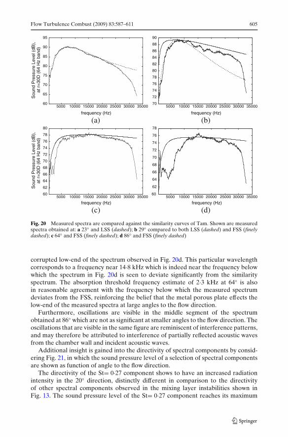
This is examined by comparing the measured spectra to the LSS and FSS spectraof Tam as shown in Fig. 20. In the figure, the peaks of the similarity spectra arepositioned to overlap the peaks of the measured spectra. Indeed, at 23◦ to theflow direction the measured spectrum matches the LSS spectrum accurately forfrequencies up to 20 kHz, after which the signal starts to deviate significantly fromthe LSS. Considering the frequency response of the Sonion microphone as depictedin Fig. 5, we may attribute the mismatch to a drop in response of the microphonefor frequencies above 20 kHz. In contrast, at 34◦ to the flow direction the recordedlow frequent pressure fluctuations confirm to the LSS spectrum but an increase inamplitude in the high-end of the spectrum causes an offset between the LSS andthe measured spectrum. The FSS spectrum is included in the figure to indicate themeasured spectrum appears to contain a combination of both.

Near 64◦ from the flow direction, the shape of the measured spectrum confirmsreasonably to the FSS spectrum. The low-end and high-end of the spectrum doesnot match the FSS spectrum. Similar to previous observations, the deviations forfrequencies above 20 kHz observed in the figure are likely due to a drop inmicrophone sensitivity to these frequencies. In comparing Figs. 20c and 20d, thediscrepancy at lower frequencies between the measured spectrum and the FSSspectrum has increased with angle. This effect may be explained by noting that thedistance between the microphone and the metal foam plate decreases with increasingangle to the flow direction, and might become comparable to the wavelength ofacoustic waves with a low frequency. The microphone at 86◦ to the flow directionis mounted approximately 2·3 cm above the metal foam plate. Given the ambientsound velocity c∞ ≈ 344 m/s and the threshold wavelength of 2·3 cm, we obtainf ≈ 14·8 kHz. Similarly, the microphone at 64◦ is mounted approximately 14·7 cmabove the horizontal, resulting in a threshold absorption frequency near 2·3 kHz. Wetherefore consider it plausible that acoustic waves with wavelengths comparable toλ = 2 · 3 cm or less are partially absorbed by the metal foam plate resulting in the


60

65

70

75

80

85

90

95

5000 10000 15000 20000 25000 30000 35000

Sou

nd P

ress

ure

Leve

l (dB

),

frequency (Hz)

70

72

74

76

78

80

82

84

86

88

90

5000 10000 15000 20000 25000 30000 35000

frequency (Hz)

(a) (b)

60

62

64

66

68

70

72

74

76

78

80

5000 10000 15000 20000 25000 30000 35000

Sou

nd P

ress

ure

Leve

l (dB

),

frequency (Hz)

60

62

64

66

68

70

72

74

76

78

5000 10000 15000 20000 25000 30000 35000

frequency (Hz)

(c) (d)

at r

=30

D (

64 H

z ba

nd)

at r

=30

D (

64 H

z ba

nd)

Fig. 20 Measured spectra are compared against the similarity curves of Tam. Shown are measuredspectra obtained at: a 23◦ and LSS (dashed); b 29◦ compared to both LSS (dashed) and FSS (finelydashed); c 64◦ and FSS (finely dashed); d 86◦ and FSS (finely dashed)

corrupted low-end of the spectrum observed in Fig. 20d. This particular wavelengthcorresponds to a frequency near 14·8 kHz which is indeed near the frequency belowwhich the spectrum in Fig. 20d is seen to deviate significantly from the similarityspectrum. The absorption threshold frequency estimate of 2·3 kHz at 64◦ is alsoin reasonable agreement with the frequency below which the measured spectrumdeviates from the FSS, reinforcing the belief that the metal porous plate effects thelow-end of the measured spectra at large angles to the flow direction.

Furthermore, oscillations are visible in the middle segment of the spectrumobtained at 86◦ which are not as significant at smaller angles to the flow direction. Theoscillations that are visible in the same figure are reminiscent of interference patterns,and may therefore be attributed to interference of partially reflected acoustic wavesfrom the chamber wall and incident acoustic waves.

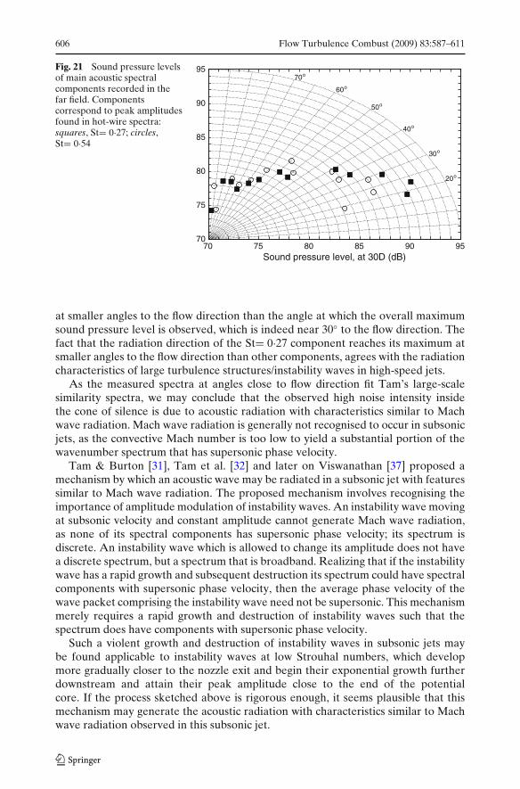
Additional insight is gained into the directivity of spectral components by consid-ering Fig. 21, in which the sound pressure level of a selection of spectral componentsare shown as function of angle to the flow direction.

The directivity of the St= 0·27 component shows to have an increased radiationintensity in the 20◦ direction, distinctly different in comparison to the directivityof other spectral components observed in the mixing layer instabilities shown inFig. 13. The sound pressure level of the St= 0·27 component reaches its maximum


Fig. 21 Sound pressure levelsof main acoustic spectralcomponents recorded in thefar field. Componentscorrespond to peak amplitudesfound in hot-wire spectra:squares, St= 0·27; circles,St= 0·54

70

75

80

85

90

95

70 75 80 85 90 95Sound pressure level, at 30D (dB)

20o

30o

40o

50o

60o

70o

at smaller angles to the flow direction than the angle at which the overall maximumsound pressure level is observed, which is indeed near 30◦ to the flow direction. Thefact that the radiation direction of the St= 0·27 component reaches its maximum atsmaller angles to the flow direction than other components, agrees with the radiationcharacteristics of large turbulence structures/instability waves in high-speed jets.

As the measured spectra at angles close to flow direction fit Tam’s large-scalesimilarity spectra, we may conclude that the observed high noise intensity insidethe cone of silence is due to acoustic radiation with characteristics similar to Machwave radiation. Mach wave radiation is generally not recognised to occur in subsonicjets, as the convective Mach number is too low to yield a substantial portion of thewavenumber spectrum that has supersonic phase velocity.

Tam & Burton [31], Tam et al. [32] and later on Viswanathan [37] proposed amechanism by which an acoustic wave may be radiated in a subsonic jet with featuressimilar to Mach wave radiation. The proposed mechanism involves recognising theimportance of amplitude modulation of instability waves. An instability wave movingat subsonic velocity and constant amplitude cannot generate Mach wave radiation,as none of its spectral components has supersonic phase velocity; its spectrum isdiscrete. An instability wave which is allowed to change its amplitude does not havea discrete spectrum, but a spectrum that is broadband. Realizing that if the instabilitywave has a rapid growth and subsequent destruction its spectrum could have spectralcomponents with supersonic phase velocity, then the average phase velocity of thewave packet comprising the instability wave need not be supersonic. This mechanismmerely requires a rapid growth and destruction of instability waves such that thespectrum does have components with supersonic phase velocity.

Such a violent growth and destruction of instability waves in subsonic jets maybe found applicable to instability waves at low Strouhal numbers, which developmore gradually closer to the nozzle exit and begin their exponential growth furtherdownstream and attain their peak amplitude close to the end of the potentialcore. If the process sketched above is rigorous enough, it seems plausible that thismechanism may generate the acoustic radiation with characteristics similar to Machwave radiation observed in this subsonic jet.


In the hydrodynamic regime in which the hot-wire measurements were taken, thedensity fluctuations may have contributions from linear and non-linear disturbances.Outside regions of exponential growth, we cannot therefore solely associate thedata with instability waves and provide direct evidence of such rapid destruction.Recent measurements of Panda & Seasholtz [25] provide some interesting trendsthat support the aforementioned mechanism. They investigated the axial variation ofdensity fluctuations along the jet centreline and along the jet peripheral mixing layer.Pressure fluctuations at low Strouhal numbers recorded with a microphone locatedclose to the jet flow direction showed significant correlation with density fluctuationsjust downstream of the end of the potential core for jets with both subsonic andsupersonic Mach numbers. This shows that the region close to the end of the potentialcore to be a low-frequency sound source for both subsonic and supersonic jets, andreinforces the notion that acoustic waves with features similar to Mach waves can begenerated in subsonic jets by amplitude modulation of instability waves.

4 Concluding Remarks

The data in this paper is considered to be suited for the validation of a DirectNumerical Simulation. Apart from the axial mean velocity distribution, we havepresented detailed information concerning the radial velocity profiles and mixinglayer thicknesses in the early stages of jet development. Such information is criticalin order to understand the manner in which the jet develops, and even more so ifpredictions made by a DNS are to be compared with experimental data obtained indownstream regions or in the far field.

Additionally, properties of the fluctuating flow field in terms of hot-wire spectraand density fluctuations were presented. The turbulence information provided inthis paper is limited to characteristics of the density fluctuations, as the hot-wire isquite insensitive to velocity and temperature fluctuations when the ambient pressuresis drastically reduced. The fluctuating flow field was characterised by the axialdevelopment of density fluctuations along the mixing layer and by documenting theirradial development at several stations along the x-axis. The fundamental mode is themost unstable mode in this jet, as became apparent by calculating the growth ratesof density fluctuations in regions of exponential growth.

The subsequent formation of its subharmonic is most interesting, as it may beexpected that vortex pairing in the jet mixing layer is an efficient noise generatingmechanism in subsonic jets. The acoustic spectra of the radiated far field show thatpressure fluctuations with frequencies near that of the subharmonic mode are themost effective noise generators in this jet.

In addition, the acoustic spectra at angles close to the flow direction were shownto be well described by Tam’s large-scale similarity spectrum, and has featuresreminiscent to that of Mach wave radiation. The evidence presented in Section 3.2indicate that subsonic jets may generate acoustic waves with characteristics similarto those of Mach wave radiation.

Acknowledgement This project is financially supported by the Dutch Technology FoundationSTW under grant number DSF:6181.


Appendix A: Hot-Wire Calibration Method

Following Perry [26], the fluctuation e′of the bridge voltage caused by a hot-wire ran

in Constant Temperature Anemometry (CTA) mode can be written in the followingform

e′

E= Au

u′

u+ Aρ

ρ′

ρ− AT

T′o

To. (6)

The coefficients Ai mentioned above can be interpreted as velocity, density and tem-perature sensitivity coefficients, respectively. To relate the hot-wire bridge voltageoutput to specific flow properties at the hot-wire probe location, the sensitivity co-efficients need be determined by means of calibration. Determining their individualvalues involves evaluating various logarithmic derivatives of parameters describingthe local heat transfer from the hot-wire to the surrounding fluid. The exact form ofthe expressions Ai are mentioned in [22], and will not be repeated here.

Any sensitivity coefficient can in principle be determined by placing the hot-wirein the laminar region of the jet and relating the hot-wire bridge output to a series ofknown flow conditions, with the restriction that the other variables remain constantduring the series of flow conditions. It may be expected that the hot-wire is mostresponsive to density changes [29], thus we shall calibrate Aρ and deduce the valuesof the two remaining sensitivity coefficients from knowledge of Aρ . For a given hot-wire overheat (τwr =(Rhot−Rcold)/Rcold), the value of Aρ can be derived from thehot-wire bridge output as function of the mean jet core density at constant jet exitvelocity and jet stagnation temperature. More specifically,

Aρ = ∂lnE∂lnρ

∣∣∣∣To,u

. (7)

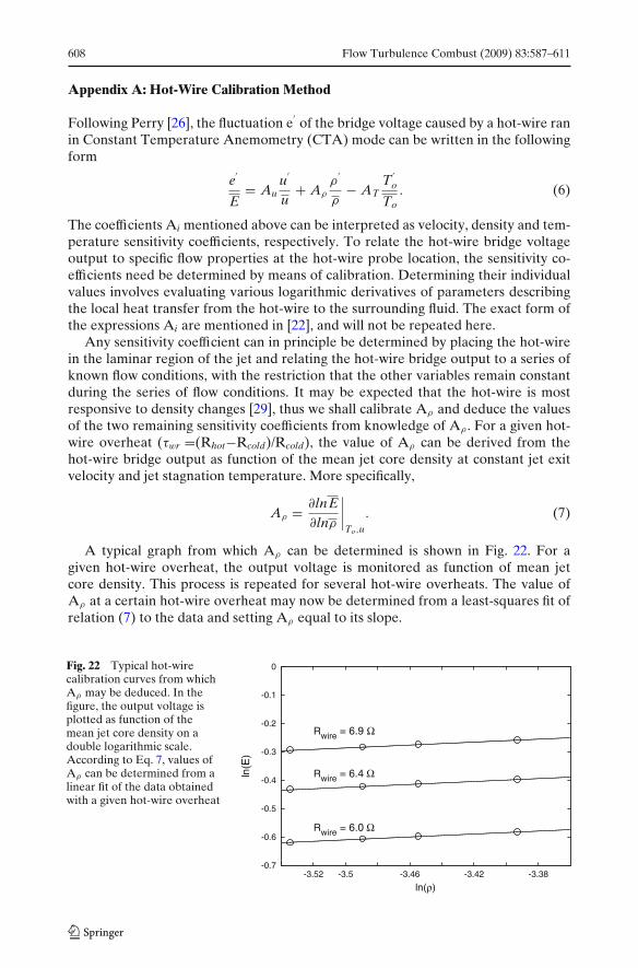
A typical graph from which Aρ can be determined is shown in Fig. 22. For agiven hot-wire overheat, the output voltage is monitored as function of mean jetcore density. This process is repeated for several hot-wire overheats. The value ofAρ at a certain hot-wire overheat may now be determined from a least-squares fit ofrelation (7) to the data and setting Aρ equal to its slope.

Fig. 22 Typical hot-wirecalibration curves from whichAρ may be deduced. In thefigure, the output voltage isplotted as function of themean jet core density on adouble logarithmic scale.According to Eq. 7, values ofAρ can be determined from alinear fit of the data obtainedwith a given hot-wire overheat

-0.7

-0.6

-0.5

-0.4

-0.3

-0.2

-0.1

0

-3.52 -3.5 -3.46 -3.42 -3.38

ln(E

)

ln(ρ)

Rwire = 6.9 Ω

Rwire = 6.0 Ω

Rwire = 6.4 Ω


All other parameters may be calculated from knowledge of Aρ . After a firstseries of measurements, the hot-wire bridge voltage fluctuations were found to beapproximately proportional to density fluctuations. Normalised fluctuations T′

rms/Tand u′

rms/u were found to contribute about 5% or less to the output and are not takeninto account.

Appendix B: Microphone Behaviour at Reduced Ambient Pressures

A model describing the sensitivity (V/Pa) of the Sonion microphones is based onparameters such as the acoustic impedance due to squeeze damping, membranestiffness and airgap volume. To understand the behaviour of the microphones atreduced ambient pressures, it is vital to recognise that the acoustic compliance ofthe airgap is linearly related to the ambient pressure

Cvol = hSγ po

[m3/Pa]. (8)

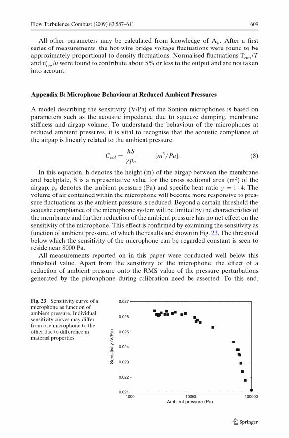
In this equation, h denotes the height (m) of the airgap between the membraneand backplate, S is a representative value for the cross sectional area (m2) of theairgap, po denotes the ambient pressure (Pa) and specific heat ratio γ = 1 · 4. Thevolume of air contained within the microphone will become more responsive to pres-sure fluctuations as the ambient pressure is reduced. Beyond a certain threshold theacoustic compliance of the microphone system will be limited by the characteristics ofthe membrane and further reduction of the ambient pressure has no net effect on thesensitivity of the microphone. This effect is confirmed by examining the sensitivity asfunction of ambient pressure, of which the results are shown in Fig. 23. The thresholdbelow which the sensitivity of the microphone can be regarded constant is seen toreside near 8000 Pa.

All measurements reported on in this paper were conducted well below thisthreshold value. Apart from the sensitivity of the microphone, the effect of areduction of ambient pressure onto the RMS value of the pressure perturbationsgenerated by the pistonphone during calibration need be asserted. To this end,

Fig. 23 Sensitivity curve of amicrophone as function ofambient pressure. Individualsensitivity curves may differfrom one microphone to theother due to difference inmaterial properties

0.021

0.022

0.023

0.024

0.025

0.026

0.027

1000 10000 100000

Sen

sitiv

ity (

V/P

a)

Ambient pressure (Pa)


consider a piston moving frictionless inside a cylinder. The process is adiabatic, andtherefore the differential relationship between p and V follows

dp = −γ pdVV

→ p′ ∝ po.

This implies there is a linear relationship between ambient pressure and theacoustic output of the pistonphone. Consequently, the p

′rms input to the microphone

during calibration can be easily calculated from its known value at standard at-mospheric conditions;

p′rms = ( pc pref

p0

) · 10SPL0/20.

In this relation, SPL0 denotes the sound pressure level of the pressure pertur-bations generated by the pistonphone at atmospheric conditions as specified bythe manufacturer and equals SPL0 = 113 · 99 dB. Furthermore, pc represents thechamber pressure (Pa), p0 is standard atmospheric pressure (Pa) and pref = 2 · 10−5

(Pa).

Open Access This article is distributed under the terms of the Creative Commons AttributionNoncommercial License which permits any noncommercial use, distribution, and reproduction inany medium, provided the original author(s) and source are credited.

References

1. Ahuja, K.K., Bushell, K.W.: An experimental study of subsonic jet noise and comparison withtheory. J. Sound Vib. 30, 317–341 (1973)

2. Batchelor, G.K.: An Introduction to Fluid Dynamics. Cambridge University Press, Cambridge(1967)

3. Bodony, D.J., Lele, S.K.: Jet noise prediction of cold and hot subsonic jets using large-eddysimulation. In: Conference paper presented at the 2004 AIAA conference, AIAA Pap. 2004–3022 (2004)

4. Boersma, B.J., Brethouwer, G., Nieuwstadt, F.T.M.: A numerical investigation on the effect ofthe inflow conditions on the self-similar region of a round jet. Phys. Fluids 10, 899–909 (1998)

5. Bogey, C., Bailly, C.: Large eddy simulations of transitional round jets: influence of the reynoldsnumber on flow development and energy dissipation. Phys. Fluids 18, 1–14 (2006)

6. Bradshaw, P.: The effect of initial conditions on the development of a free shear layer. J. FluidMech. 26, 225–236 (1966)

7. Bradshaw, P., Ferriss, D.H., Johnson, R.F.: Turbulence in the noise-producing region of a circularjet. J. Fluid Mech. 19, 591–624 (1963)

8. Crow, S.C., Champagne, F.H.: Orderly structure in jet turbulence. J. Fluid Mech. 48, 547–591(1971)

9. Deo, R.C., Mi, J., Nathan, G.J.: The influence of reynolds number on a plane jet. Phys. Fluids 20,075108 (2008). doi:10.1063/1.2959171

10. Freund, J.B.: Noise sources in low-reynolds-number turbulent jet at mach 0·9. J. Fluid Mech. 438,277–305 (2001)

11. Hussain, A.K.M.F.: Coherent structures—reality and myth. Phys. Fluids 26, 2816–2850 (1983)12. Hussein, H.J., Capp, S.P., George, W.K.: Velocity measurements in a high-reynods-number,

momentum-conserving, axisymmetric, turbulent jet. J. Fluid Mech. 258, 31–75 (1994)13. Ko, C.L., McLaughlin, D.K., Troutt, T.R.: Supersonic hot-wire fluctuation data analysis with a

conduction end-loss correction. J. Phys. E: Sci. Instrum. 11, 488–494 (1978)14. Laufer, J., Kaplan, R.E., Chu, W.T.: Acoustic modeling of the jet noise abatement problem. In:

Proc. Interagency Symp. on University Research in Transportation Noise, Stanford, 28–30 March1973

15. Laufer, J., Yen, T.: Noise generation by a low-mach-number jet. J. Fluid Mech. 134, 1–31 (1983)

http://dx.doi.org/10.1063/1.2959171


16. Lush, P.A.: Measurement of subsonic jet noise and comparison with theory. J. Fluid Mech. 46,477–500 (1971)

17. McLaughlin, D.K., Morrison, D.K., Troutt, T.R.: Experiments on the instability waves in asupersonic jet and their acoustic radiation. J. Fluid Mech. 69, 73–95 (1975)

18. Michalke, A.: On spatially growing disturbances in an inviscid shear layer. J. Fluid Mech. 23,521–544 (1965)

19. Michalke, A.: Survey on jet instability theory. Prog. Aerosp. Sci. 21, 159–199 (1984)20. Mollo-Christensen, E., Kolpin, M.A., Martucelli, J.R.: Experiments on jet flows and jet noise

far-field spectra and directivity patterns. J. Fluid Mech. 18, 285–301 (1964)21. Moore, P.D., Slot, H.J., Boersma, B.J.: Simulation and measurement of flow generated noise. J.

Comput. Phys. 224, 449–463 (2007)22. Morkovin, M.V.: Fluctuations and hot-wire anemometry in compressible flows. AGARDograph

24 (1956)23. Oneill, P.L., Nicolaides, D., Honnery, D., Soria, J.: Autocorrelation functions and the determi-

nation of integral length with reference to experimental and numerical data. Fluid MechanicsConference, Sydney, 13–17 December 2004

24. Panchapakesan, N.R., Lumley, J.L.: Turbulence measurements in axisymmetric jets of air andhelium. Part 1. Air jet. J. Fluid Mech. 246, 197–223 (1993)

25. Panda, J., Seasholtz, R.G.: Experimental investigation of the density fluctuations in high-speedjets and correlation with generated noise. J. Fluid Mech. 450, 97–130 (2002)

26. Perry, A.E.: Hot-Wire Anemometry. Oxford University Press, Oxford (1982)27. Quadrio, M., Luchini, P.: Integral space-time scales in turbulent wall flows. Phys. Fluids, 15, 2219–

2227 (2003)28. Schram, C., Taubitz, S., Anthoine, J., Hirschberg, A.: Theoretica/emperical prediction and mea-

surement of the sound produced by vortex pairing in a low mach number jet. J. Sound Vib. 281,171–187 (2005)

29. Stromberg, J.L., McLaughlin, D.K., Troutt, T.R.: Flow field and acoustic properties of a machnumber 0.9 jet at a low reynolds number. J. Sound Vib. 72, 159–176 (1980)

30. Swamy, N.V.C., Gowda, B.H.L., Lakshminath, V.R.: Auto-correlation measurments and integraltime scales in three-dimensional turbulent boundary layers. Flow Turbul. Combust. 35, 237–249(1979)

31. Tam, C.K.W., Burton, D.E.: Sound generated by instability waves of supersonic flows. Part 2.Axisymmetric jets. J. Fluid Mech. 138, 273–295 (1984)

32. Tam, C.K.W., Golebiowski, M., Seiner, M.: On the two components of turbulent mixing noisefrom supersonic jets. AIAA Pap. 96 (1996)

33. Tam, C.K.W., Morris, P.J.: The radiation of sound by the instability waves of a compressibleplane turbulent shear layer. J. Fluid Mech. 98, 349–381 (1980)

34. Tanna, H.K.: An experimental study of jet noise, part 1: turbulent mixing noise. J. Sound Vib.50, 405–428 (1977)

35. Troutt, T.R., McLaughlin, D.K.: Experiments on the flow and acoustic properties of a moderate-reynolds-number supersonic jet. J. Fluid Mech. 116, 123–156 (1982)

36. VanderHeggeZijnen, B.G.: Measurements of the velocity distribution in a plane turbulent jet ofair. Appl. Sci. Res. 7, 256–276 (1958)

37. Viswanathan, K.: Aeroacoustics of hot jets. J. Fluid Mech. 516, 39–82 (2004)38. Wygnanski, I., Fiedler, H.: Some measurements in the self-preserving jet. J. Fluid Mech. 38, 577–

612 (1969)39. Zaman, K.B.M.Q.: Effect of initial condition on subsonic jet noise. AIAA J. 23(9), 1370–1373

(1985)40. Zaman, K.B.M.Q.: Flow field and near and far sound field of a subsonic jet. J. Sound Vib. 106,

1–16 (1986)

Documents

Experiments on the Flow Field and Acoustic Properties of a