1

EXPERT REVIEW OF

“Methodology Analysis for Weighting of Historical Experience”

Prepared by National Crop Insurance Services, Inc.

October 17, 2011

Executive Summary

On September 17, 2011, the Risk Management Agency (RMA) of the U.S. Department of Agriculture

requested National Crop Insurance Services (NCIS) to prepare an expert review of the Sumaria Systems

study entitled “Methodology Analysis for Weighting of Historical Experience." The purpose for the

Sumaria study was to evaluate and recommend improvements to RMA’s current ratemaking

methodology.

In conducting this review, it is imperative to state that the primary objective of our review was to

determine if the newly proposed procedure is the product of sound analytical and empirical technique and

that the resulting estimates are technically accurate and can be reliably replicated.

In general, NCIS finds that the ratemaking study is not governed by the formal development of an

analytical framework which can be used to systematically estimate the relationship between crop

insurance loss data and the appropriate weighting of such data in the context of climate experience.

Rather, the Sumaria study represents a conglomeration of numeric computations yielding a set of

proposed crop insurance premium rates which cannot readily be verified or replicated based on the

information provided to our review team. Our major concern rests not with the direction of the proposed

premium changes, rather it is the magnitude of the proposed changes relative to current practice and the

weaknesses of the approach used to generate the proposed premium changes.

With respect to substantive issues detailed in our review, we highlight the following here.

(1) Adherence to Actuarial Standards of Practice: The study does not adequately adhere to the practice

of prospective ratemaking, but rather the computations (by reducing the time period for base-rate setting)

reflect a financial recoupment process which will likely result in more variable rate-setting over time.

2

(2) Econometric Considerations: It is not apparent from our review that formal econometric model

specification and selection criteria were systematically applied throughout the study. In addition, current

empirical literature does not appear to be adequately cited. Empirical evidence from this literature

actually challenges a fundamental and major data adjustment computation used in the study, specifically,

the "Pre-1995" effect.

(3) Empirical Deficiencies: Several of the numeric computations can be successfully challenged. The

"Bin Probability" computation does not appear to provide any "statistical validity" or improve the

performance of the proposed rate-setting procedure. The statistical properties of the Weather-Weighting

computation can also be seriously questioned (this is technically demonstrated in our review). The study

also lacks an explanation for how the use of the same historical data as the current ratemaking method

results in vastly different rates. This should be of serious concern to USDA / RMA and all program

stakeholders. Before proceeding further, this issue probably deserves the most attention. It is

conspicuously absent from the Sumaria study.

As important as the technical aspects of the study, our review addresses both operational and program

issues associated with the study. Major changes to RMA's actuarial methodology and processes are not

simply a technical actuarial and statistical issue. Major changes impact the delivery system, such as

impacts to the USDA baseline, potential market disruption due to volatile premium rate setting by RMA,

and Standard Reinsurance Agreement (SRA) impacts on private sector delivery. Although beyond the

scope of the Sumaria study, awareness of these potential impacts should be an element of the Expert

Review process. We have included a section on these issues in our review.

It would have been desirable to have more time to review the study, as well as access to additional data.

However, we are confident with the quality of our review. The NCIS review team recommends that the

proposed rates and the underlying methodology not be implemented in any form whatsoever. In our

view, if the proposed ratemaking methodology is implemented by USDA / RMA, it will not have been on

the basis of its technical or analytic merits. The Federal crop insurance program is responsible for

determining and setting actuarially fair and reasonable premium rates for US farmers and ranchers. This

principle cannot be overstated or over-emphasized. It is unfortunate that the proposed results and

methodology do not allow for an accurate determination of actuarially fair and sound premium.

Brief biographies of the individuals participating in the expert review are provided at the end of this

report.

3

Introduction

On September 17, 2011, the Risk Management Agency (RMA) of the U.S. Department of Agriculture

requested National Crop Insurance Services (NCIS) to prepare an expert review of the Sumaria Systems

study entitled “Methodology Analysis for Weighting of Historical Experience.” This study consists of

two reports, “Revised Technical Report July 12, 2011” and “Implementation Report September 5, 2011.”

The purpose for the Sumaria study was to evaluate and recommend improvements to RMA’s current

ratemaking methodology. The response provided herein provides the NCIS Expert Review in its entirety.

This report consists of an Executive Summary, followed by this introduction, a review of the relevant

actuarial principles, an evaluation of the econometric issues, a review of the empirical deficiencies of the

study, and a discussion of the operational issues. The final section of this review provides our assessment

of the study and recommended actions to be taken by RMA. Biographies of the individuals participating

in the expert review and a technical appendix are provided at the end of this report.

While specific comments regarding the study are provided in the body of this report, a few general

observations should be made with regard to the study and the process of conducting the review. First, it is

important to recognize that NCIS has been able to examine only a portion of the study. The Expert

Review process provides each reviewer only a limited amount of written documentation and extremely

limited access to the data and the analysis underlying the study. Since the study has been ongoing over

the past year, it would have been beneficial if RMA had brought NCIS, the industry, and potentially other

reviewers into the process at an earlier date in order to ensure adequate time to examine the study in

depth. In conducting its expert review, NCIS requested a small amount of supporting information from

the contractors via RMA. While we were unable to obtain everything we requested, the contractors

responded to our request, although the data provided was not at the appropriate level of detail to make it

possible to conduct a thorough analysis. Despite this, we feel confident in the data obtained and in the

written documentation to be able to provide a reasonably thorough evaluation of the proposed ratemaking

methodology.

In general, NCIS finds that the ratemaking study suffers from the absence of a formal model being tested

and, as a result, is lacking in analytical rigor. A detailed examination of the relevant actuarial

considerations, econometric issues, and empirical deficiencies is provided in our response. The selected

ratemaking methodology relies on a variety of assumptions and adjustments, many of which seem ad hoc.

Several adjustments may target the same issue, such as the use of multiple methods to dampen the effect

of large losses in the older years on the indicated rates. Furthermore, the results of the study are not

4

robust – the indicated rates depend strongly on which set of adjustments and methods are applied. In

more practical terms, this means that the rates might have been much higher or lower if other assumptions

had been used. The absence of a formal peer review of the study adds to our concern about its reliability.

The study also lacks an explanation for how the use of the same historical data as the current ratemaking

method results in vastly different rates. For these and other reasons, we have no confidence whether the

proposed rates are accurate or not. We are confident, however, that the proposed ratemaking

methodology is not reliable.

5

Overview of Proposed Methodology

From a broad perspective, the proposed ratemaking methodology modifies rather than replaces RMA’s

current ratemaking procedure. Similar to the existing approach, rates are developed on a bottom-up basis,

separately by county, rather than using a top-down approach that would allocate a statewide rate change

to the individual counties. Within that framework, the proposed methodology makes a number of

significant changes to the individual steps in the current process. While the documentation of the study is

not organized in a manner conducive to understanding every step of the process, the following

summarizes our interpretation of how the new methodology operates.

The initial step in the process is to convert the loss costs to a common coverage level. Then, an

evaluation is performed to estimate how changes in the program over time have affected the loss costs.

The study divides the historical experience into two periods, 1975-1995 and 1995-current and develops an

estimate of the adjustment needed on a nationwide basis to convert the experience from the earlier period

to the level expected under the current program. The selection of 1995 as the break point has been

justified on the basis of program changes and a sharp increase in program participation at that time. The

nationwide adjustment is subsequently allocated to states in some manner.

Next, the adjusted loss cost experience is aggregated to the Climate District level. Climate districts are

extended areas somewhat akin to crop reporting districts. Each Climate District has 116 years of

historical weather data. The weather variables considered in this study include the Palmer Drought

Severity Index (for specific time periods, separately for negative and positive values of the index) and

Cooling Degree Days (for the entire growing season as well as portions of the season). The study limits

the number of dependent variables to seven. Next, Climate District weather data from 1975 forward is

combined with the insurance experience. A fractional logit regression of the adjusted loss cost data is

then performed to construct weather indices from 1895 to the present. Within each Climate District, the

resulting 116 weather index values are then grouped into a series of bins with each having roughly an

equal number of observations, representing equal probabilities. The binning process is then applied to

each county within the Climate District based on the county’s weather indices over the most recent 20

year period. The number of bins selected for a county can range from 5 to 15, based on a goal of using as

many bins as possible, provided that each bin has at least a single observation. If fewer than 5 bins are

indicated, weather weighting is not used. The assignment of years to bins is used to determine the

assignment of loss costs to the corresponding bins.

6

At this point the loss costs are split into their normal and catastrophic components. Normal loss costs are

obtained by capping total loss costs at the 90th percentile of the county loss cost distribution, an increase

over the 80th percentile used in the current procedure. Only the most recent 20 years of normal loss costs

are included in the binning procedure. If more than one observation is included in a bin, an acre

weighting process is used to determine the average value for that bin. A simple average of the loss costs

across bins is used to determine the normal loss cost for the county.

The study uses all of the available years of data (1975 to present) in the development of the catastrophic

component of the county rate. By construction, only 10% of the years (10% of 35 years) are classified as

having a catastrophic loss. To develop the catastrophic component of the county rate, the procedure first

determines if the weather index for any year in the experience period is in the top 3% of the entire set of

116 weather index values. If no observation falls within the top 3%, each value is given equal weight.

For any year within the top 3%, a factor is applied to reduce the losses under the theory that the weather

in that year was highly unusual.

7

Actuarial Issues and Principles

The Proposed Ratemaking Methodology Fails to Meet Actuarial and Legislated Standards

Part 1 – The 20 Year Experience Period

The proposed ratemaking methodology raises a number of concerns regarding whether the methodology

and the indicated rates are consistent with actuarial ratemaking principles. The Casualty Actuarial

Society “Statement of Principles Regarding Property and Casualty Insurance Ratemaking”

(http://www.casact.org/standards/princip/sppcrate.pdf) states the following:

Ratemaking is prospective because the property and casualty insurance rate must be developed

prior to the transfer of risk.

Principle 1: A rate is an estimate of the expected value of future costs.

Similarly, sections 1508(d)(1) and (2) of the Crop Insurance Act require FCIC to establish premiums

sufficient to cover anticipated losses and a reasonable reserve. It should be noted that both standards, one

embedded in legislation and the other a basic principle of actuarial ratemaking, refer to the rates or

premiums being implemented rather than to the ratemaking methodology used to develop those rates or

premiums. The critical issue is whether the ratemaking methodology proposed by this study is capable of

satisfying these objectives. It is not.

In order to understand why the method fails to meet the actuarial and legal standards, a brief overview of

the methodology is essential. Under the proposed ratemaking procedure, losses for individual years are

capped at the 90th percentile of the county loss costs. Two distinct approaches for developing the capped

and excess portions of the proposed rates are then employed. With regard to the capped portion of the

rate, the procedure is based on the most recent twenty years of loss experience. The point to be

considered here is whether it is appropriate to use only the most recent 20 years of capped loss costs or

whether all years of data should be included in the analysis.

We note that the contractor has previously rejected the use of a pre-specified experience period in its

response to one of the expert reviews of its Comprehensive Review of the RMA ratemaking

methodology. The relevant section of the response states:

8

“Any arguments (along with their supporting statistical tests) that make sweeping statements

based upon conveniently-defined periods of study (e.g., 1980-2008) and that present probability

values from formal statistical tests conducted while ignoring many of these complicating factors

(as well as many other conditions that further complicate formal statistical inference) are

suspect.”

In evaluating the ratemaking methodology, it is important to recognize that crop insurance rates are

established from a bottom-up manner, separately by crop and county. This differs from more traditional

actuarial ratemaking methods that operate on a top-down basis, starting with a statewide rate indication

and using an allocation process to spread the statewide rate change in a seemingly reasonable manner to

all territories within the state. The inherent conflict of actuarial techniques with actuarial principles is not

readily apparent when using the traditional top-down approach, but is a critical issue when rates are

established using a bottom-up approach as in crop insurance. The distinction arises out of the high

variability of county data in relation to the relatively stable and predictable experience observed on a

statewide basis for most types of Property and Casualty insurance. Even capping losses at the 80th or

90th percentile can be ineffective at resolving the problem in that the capped loss costs are still highly

variable (as measured by their coefficient of variation, for example).

The problem can be easily illustrated by considering an insurance program having low likelihood of a

severe loss. While this is a simplified example, the concept applies equally well to the proposed

ratemaking methodology. Loss capping is disregarded in order to simplify the discussion. Assume that

the loss cost is 10 in normal years (years 1 through 9) and 50 in the tenth year, and similarly in future

years. In this example, the expected loss cost is equal to the long-term average loss cost of 14. Now

consider an insurer that begins to offer coverage starting in year 6. Suppose that the insurer employs a

ratemaking procedure that uses a five year experience period so that each year’s rates are equal to the

average loss cost over the prior five years. Over the long term, this results in a rate of 10 for the first five

years, followed by a rate of 18 over the next five years. This pattern continues to repeat over time.

However, at no time does this method establish a rate equal to the long-term expected loss cost of 14.

Instead, it alternates between an inadequate rate of 10 and an excessive rate of 18. In other words, the

insurer experiences a significant loss in one year out of 10 and attempts to recoup the loss by

overcharging its policyholders over the following five years. Not only does this ratemaking approach

clearly fail to set the rate at the expected value of future costs, it also fails to meet the actuarial

requirement that rates be established on a prospective basis. This methodology can be more accurately

described as a recoupment process. This should be apparent to anyone working in the Property and

9

Casualty insurance industry. The Florida Homeowners insurance market provides a clear example of

what may occur if rates are based on insufficient history. Prior to Hurricane Andrew in 1992, insurers

failed to include an appropriate loading for hurricane losses in their rates due the lengthy period since the

previous landfall along the Florida coast, leading to severe market disruptions that continue to the present

day.

The Property and Casualty industry differs from crop insurance in that P&C insurers have the ability to

recoup underwriting losses reasonably quickly due to their control over their own rates, prices, and

underwriting decisions. Crop insurers, on the other hand, have no ability to recoup their prior losses.

Recognizing this, Congress established a requirement that rates be set at the anticipated level of losses

rather than through the use of a recoupment mechanism. This helps to ensure that participating insurers

are able to build adequate financial reserves in advance of a catastrophic year in recognition of their

inability to recoup those losses in future years. This also serves to ensure the financial stability of

participating insurers, particularly in light of the catastrophic nature of the risk. However, due its use of a

20 year experience period, the proposed methodology operates as a recoupment method rather than a

prospective pricing method. This inability to set rates at the anticipated level of losses means that the

methodology is fundamentally incompatible with the Congressional objective. As a result, participating

insurers would be incapable of building adequate reserves in advance of a catastrophic year, which could

threaten the financial stability of the delivery system.

The question of whether the proposed methodology reflects the true risk of the program also appears in

regard to the impact of climate change on the program. It is troublesome that a procedure based on

weather modeling would fail to account for climate change in its estimation of the rates, or at a minimum

acknowledge the issue in the context of the overall study.

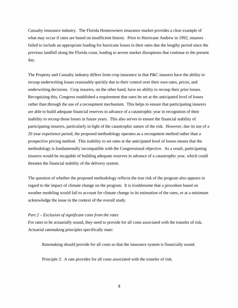
Part 2 – Exclusion of significant costs from the rates

For rates to be actuarially sound, they need to provide for all costs associated with the transfer of risk.

Actuarial ratemaking principles specifically state:

Ratemaking should provide for all costs so that the insurance system is financially sound.

Principle 2: A rate provides for all costs associated with the transfer of risk.

10

An insurer’s costs include the indemnities paid to policyholders, expenses related to the delivery of

policies to policyholders, the cost associated with the adjustment of claims, as well as the cost of

operating the insurance company. The rationale behind the principle stated above is that insurers need to

obtain an adequate return for the risk they take. If premiums are insufficient to cover an insurer’s

expenses, its return would be reduced below the acceptable level. This increases the difficulty of raising

capital, reduces the incentive for new insurers to enter the market, and may lead existing insurers to

reduce capacity or withdraw from the market. As financial professionals, actuaries have a responsibility

to ensure the financial stability of the insurance industry. In that regard, we would expect that a

ratemaking methodology change that leads to substantial reductions in the rates would be given extensive

scrutiny to ensure that the program continues to operate on a financially sound basis. We have serious

reservations in that regard. The following discussion highlights several of our major concerns.

Property and Casualty insurers are generally responsible for setting their own rates. This gives each

company the ability to include an appropriate loading for profit and expense in its rates. However, this

does not apply to the Federal crop insurance program. Instead, each participating insurer is required to

use the rates developed by RMA. Since RMA’s rates exclude any provision for profit or expense, this

raises the question of whether the proposed rates are consistent with the actuarial principle that all costs

associated with the transfer of risk are addressed. Three basic concerns are the adequacy of A&O

reimbursements to cover industry operating costs, the cost of commercial reinsurance, and the cost of

reinsurance provided through the SRA.

In recognition of the fact that crop insurance rates exclude any loading for profit and expense, the SRA

provides an alternative reimbursement method, referred to as A&O reimbursements, as a mechanism to

compensate companies for their policy delivery, claim adjustment, and other operating expenses.

However, reimbursements have been insufficient to cover the full cost for more than a decade. In

addition, due to the explicit cap on A&O reimbursements imposed by the 2011 SRA, A&O shortfalls are

expected to continue in future years.

The second expense issue relates to the cost of commercial reinsurance purchased through the private

market. Insurers purchase commercial reinsurance to stabilize their results and to protect their surplus

against catastrophic events. Similar to any other product or service, reinsurance has a cost to the

purchaser. In the case of the crop insurance industry, government regulations impose an additional cost

on companies in terms of capital requirements. The purpose of the regulation is to ensure company

solvency by requiring participating insurers to maintain extremely high levels of surplus (surplus must be

11

at least twice the maximum possible underwriting loss, or roughly twice the insurer’s retained premium).

The relevance of this regulation is that financial theory states that investors will demand that insurers

achieve a return commensurate with the capital being held. From a different perspective, capital imposes

a cost on the insurer in that investors need to be compensated for the use of their capital. If the insurer is

unable to generate a sufficient return on its book of business, capital would be withdrawn and the ability

to deliver the program would be compromised.

In the interest of encouraging private sector participation in light of the program’s onerous capital

requirements, RMA allows companies to use external reinsurance as a substitute for maintaining large

capital reserves in their surplus accounts. Since the demand for additional reinsurance is the result of

government capital requirements rather than in response to business needs, the additional protection has

limited value to insurers. Instead, the benefits accrue primarily to the government by reducing the need to

compensate investors adequately for use of their capital, as well as to producers by increasing the

availability of coverage. Despite this, the cost of reinsurance is borne entirely by the private sector.

Companies are not compensated for this cost either through the A&O reimbursement mechanism or the

rates. However, standard actuarial ratemaking practices emphasize the need to address all costs in order

to ensure financial soundness and stability of the insurance system.

The third item, the cost of reinsurance provided through the SRA, provides another perspective on the

conflict with actuarial ratemaking principles. This imposes an unavoidable expense on every insurer

participating in the program. During the recent SRA negotiations RMA provided estimates of industry

underwriting gains under both the 2005 and 2011 SRAs. These estimates were developed without

consideration of the rate changes now being proposed. Given the magnitude of the proposed rate

reductions, we believe that future underwriting gains will be reduced substantially, and that this will have

a material impact on the financial soundness of the insurance system.

Part 3 – Impact on the Financial Soundness of the Program

Promoting the financial soundness of the insurance system is a fundamental principle of the actuarial

profession. In light of that, a decision to drastically modify rates for the two largest crops without

correcting for deficiencies throughout the rest of the program will materially affect the overall financial

soundness of the program. We find it troubling that large reductions are being proposed for immediate

implementation while any increases are being delayed until a future date.

12

Technical Considerations

Credibility

Traditionally, actuarial ratemaking techniques take into consideration the credibility of the experience.

Credibility methods are applied in two ways. First, credibility is used to moderate the statewide rate

indication from one review to the next. Second, credibility is used to stabilize rate changes for individual

territories. Neither of these is addressed directly in the proposed ratemaking methodology. However, the

use of acre weighting in evaluating the loss cost in each weather bin, along with the limitation of the

experience period to 20 years can be considered to be indirect techniques for addressing the credibility of

the experience.

Acre weighting is used in the proposed methodology to give less weight to the experience for years in

which a smaller area was insured. This would be appropriate if the credibility of the experience were

related to the area insured. However, the Sumaria actuary stated during an August 2011 presentation to

industry that individual counties behave in a manner similar to individual exposures. In effect, the

actuary was stating that insuring additional acreage within a county adds little to the credibility of the

experience. One way to test whether credibility is related to the area insured is by observing that acreage

has increased steadily over time. As a result, the assumption that credibility depends on area is equivalent

to the assumption that recent experience is more indicative of future results than is experience from earlier

years. This can be evaluated through the use of an exponential weighting model. This model has the

advantage that its forecasting model is identical to the traditional actuarial credibility formula. In

conducting this test, we found that each year should be assigned essentially the same weight. Two

conclusions can be drawn from this. First, it demonstrates that credibility is unrelated to the area insured.

Second, it implies that the straight average of the historical loss costs provides a better estimate of future

results than the assignment of greater weights to more recent years. The use of an unweighted average

including all years has the added benefit of stabilizing the rates from one review to the next. From a

ratemaking perspective, this indicates that all years of data should be included rather than limiting the

experience to the most recent 20 years. From this, we draw the conclusion that all years of data need to

be included in the ratemaking procedure and that each year should be given equal weight in the analysis.

A different way to evaluate the credibility of the experience is to apply the Longley-Cook technique (see

http://www.casact.org/pubs/proceed/proceed62/62194.pdf). The traditional actuarial standard for full

credibility is the number of observations needed in order for the sample mean to be within 5% of the true

13

mean with a probability of 90%. Based on the observed coefficient of variation over the period from

1980 through 2010 for corn loss costs (CV = 1.73) in a typical Iowa county, more than 3,200 years of

experience are needed to reach full credibility. This strongly supports the notion that all available years

of data need to be included in establishing crop insurance rates.

The use of acre weighting is in direct conflict with the fundamental basis of the study itself. The study

focuses on weather as a primary driver of the loss experience. Since weather is a systematic risk affecting

large areas within a county simultaneously, the average loss cost based on a large insured area should be

reasonably similar to the loss cost for a smaller area. The implication of the weather model is that the size

of the area insured is unrelated to the credibility of the loss experience.

The discussion of credibility in the preceding paragraphs is not intended to suggest that RMA should

revise its ratemaking procedures to conform to traditional actuarial credibility methods. The reason this is

unnecessary is that RMA already applies a theoretically valid actuarial credibility method in its county

loss cost smoothing procedure. We encourage RMA to continue the use of county loss cost smoothing in

the future to ensure the accuracy of county rates.

Rationale for the Pre-1995 Adjustment

In its discussion of the non-stationarity of historical loss costs, the study identifies 1995 as the point at

which the experience under the program underwent a significant change. The authors noted that this

“corresponds to known changes in the way the program was administered and to a marked increase in

program participation.” The study presented a chart illustrating the large increase in insured acres starting

in 1995. Our interpretation is that the primary reason for selecting 1995 as the breakpoint was due to the

belief that the new exposures entering the program had much better loss experience than the exposures

insured in earlier years. In effect, the large increase in exposures was considered to have eliminated the

problem of adverse selection against the program.

The difficulty with the rationale stated above is that virtually all of the increase in acreage was due to the

introduction of the CAT program. The following chart is similar to the chart shown on page 22 of the

final report, but breaks out the acreage between CAT and all other business. The rest of the program

(indicated by the red Buy-up curve) showed no significant increase in volume in 1995. Instead, Buy-up

acreage has increased gradually over the history of the program. This would argue against a dramatic

reduction in adverse selection in the Buy-up segment of the program occurring around 1995. This is

relevant because, based on our understanding of the current ratemaking methodology, rates are developed

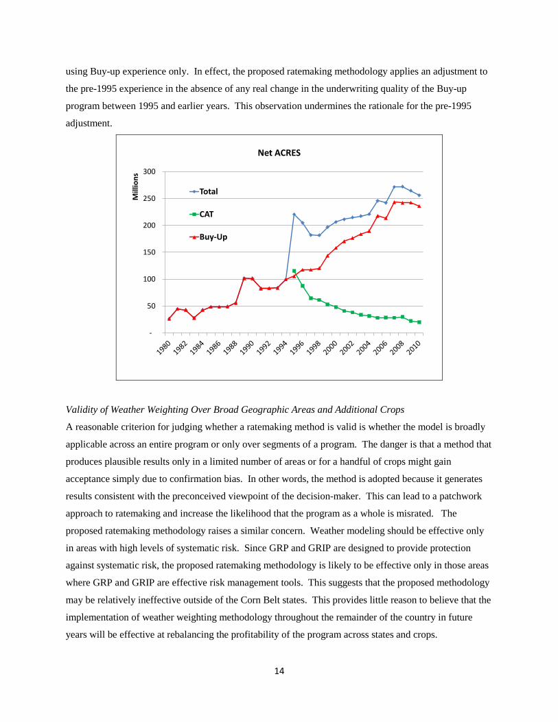
14

using Buy-up experience only. In effect, the proposed ratemaking methodology applies an adjustment to

the pre-1995 experience in the absence of any real change in the underwriting quality of the Buy-up

program between 1995 and earlier years. This observation undermines the rationale for the pre-1995

adjustment.

-

50

100

150

200

250

300

Mill

ions

Net ACRES

Total

CAT

Buy-Up

Validity of Weather Weighting Over Broad Geographic Areas and Additional Crops

A reasonable criterion for judging whether a ratemaking method is valid is whether the model is broadly

applicable across an entire program or only over segments of a program. The danger is that a method that

produces plausible results only in a limited number of areas or for a handful of crops might gain

acceptance simply due to confirmation bias. In other words, the method is adopted because it generates

results consistent with the preconceived viewpoint of the decision-maker. This can lead to a patchwork

approach to ratemaking and increase the likelihood that the program as a whole is misrated. The

proposed ratemaking methodology raises a similar concern. Weather modeling should be effective only

in areas with high levels of systematic risk. Since GRP and GRIP are designed to provide protection

against systematic risk, the proposed ratemaking methodology is likely to be effective only in those areas

where GRP and GRIP are effective risk management tools. This suggests that the proposed methodology

may be relatively ineffective outside of the Corn Belt states. This provides little reason to believe that the

implementation of weather weighting methodology throughout the remainder of the country in future

years will be effective at rebalancing the profitability of the program across states and crops.

15

Econometric Issues

The Contractor’s Econometric Analysis Regarding the Relationship between Loss Cost and

Weather Variables Has Serious Flaws

It is standard practice in econometric analysis or statistical estimation to properly specify the model being

estimated and to assign a priori expectations to parameter estimation. Our review finds the technical

report conspicuously lacking in this regard. Improper model specification will result in biased estimators,

which in turn result in an over or under estimation of the predicted values, depending upon the nature of

the bias.

Due to ill-defined specification, we cannot ascertain if the empirical output of the model is reliable. We

believe our discussion in this section of our review more than adequately demonstrates our concerns.

Statistical Validity

The contractor states the objective of their study as “The statement of work also directed us to deliver a

report that offers multiple approaches that compare and contrast the varying combinations of the factors

based on statistical validity, feasibility, sustainability, and a balance of improvement versus complexity”

(see p.3 of the September 5 report) and “adjusting RMA’s historical loss cost data in order to maximize

its statistical validity for developing premium rates” (see p. 82 of the September 5 report). The contractor

applies the term “statistical validity” ten times in their combined reports without providing a formal

definition or criteria for determining it.

Econometric Model Specification

The contractor uses Cooling Degree Days (CDD) variables and Palmer Draught Severity Index (PDSI) as

the explanatory variables. However, there are significant issues arising from: (1) inadequate specification

of the included variables; and (2) omitted variables, which will be reviewed as follows.

1. Problems with the Included Variables

CDD variables are the cumulative sum of degree days or heat units that are beneficial for crop growth.

The CDD variables used in the contractor’s analysis are total season CDD (from May to September) and

June-July total CDD.

16

One immediate observation is that total season CDD variable includes the impact of June-July total CDD

variable, which may affect the results of the regression. Alternatively, the contractor could split the Total

season CDD variable into three variables: May total CDD, June-July total CDD, and August-September

total CDD.

The formulation of the CDD variables is not consistent with the literature. Both Schlenker and Roberts

(2008); and Vado and Goodwin (2010): (1) put a lower bound and an upper bound for CDD variable

within which temperature is assumed to be beneficial for the plant growth; and (2) define a separate

variable for the temperatures beyond upper threshold, which is called Harmful Degree Days (HDD)

variable. This was not addressed by the contractor.

The contractor uses 65° F (18.3°C) as their lower bound in their CDD variable, that is, they set degree

days to zero at this temperature. In comparison, Schlenker and Roberts; and Vado and Goodwin set the

lower threshold at 46.4° F (8° C). The appropriate bounds for growing degree days is still debatable

(Schlenker and Roberts). Nevertheless, the contractor’s choice is significantly different than the literature

suggests. For all temperatures between 46.4° F and 65.3° F, the contractor sets the CDD variables to zero.

Another issue with the CDD variables is the contractor did not specify an upper bound for CDD variables.

Schlenker and Roberts find that yields increase up to 84.2° F (29° C) for corn, 86° F (30° C) for soybeans,

and 89.6° F (32° C) for cotton. The temperatures beyond these levels are harmful to the crops. Indeed,

they also find that the slope of decline in yield after passing the upper bound temperature is steeper than

the incline before it (known as non-linearity of yields in temperature).

Schlenker and Roberts; and Vado and Goodwin construct a separate variable for high temperatures: called

heating (harmful) degree days (HDD) which is the cumulative sum of degree days or heat units that are

harmful for crop growth, higher than some threshold level, which are 86°F (30°C) in Vado and Goodwin,

and 93° F (34° C) in Schlenker and Roberts. Instead, the contractor fails to address the established result

of non-linearity between yields and weather variables (Schlenker and Roberts; Vado and Goodwin). The

contractor cites some other literature and states that drought is the major cause of losses and yet they do

not properly account for the extreme heat variable extended over a period of time. Schlenker and Roberts

construct the HDD variable as the deviation from its mean and find it statistically significant. Vado and

Goodwin find statistically significant HDD variables with positive signs in their loss cost estimations.

17

Note that the CDD variables are chosen as the “best” weather variables by the contractor in 19 out of 56

states (including Iowa, Illinois, Indiana) and are among the “best” weather variables (together with PDSI

variables) in additional four states. A misspecification regarding the CDD variable will surely affect the

accuracy of the loss cost estimates.

Beyond the aforementioned issues with the variables, the contractor limits their analysis to seven

combinations of the CDD variables and PDSI variables by citing the computational burden. These

combinations are not exhaustive and not chosen based on statistical significance tests.

2. Problems Arising From Excluded (Omitted) Variables

The contractor omits some important variables despite these variables being identified as significant in the

literature. Omitted significant variables would make the predicted loss costs biased and the estimation

may have large errors, therefore, the resulting bases rates could be biased, inefficient and less accurate.

The contractor omits factors such as freeze (an important cause of loss for other crops such as sugar beet)

or flooding which may be caused by excessive moisture in another location. Moreover, the contractor

does not control for (include) local soil types. Vado and Goodwin; and Schlenker and Roberts find

significant location specific unobserved effects (fixed effects).

The contractor also does not control for a technological change variable. Vado and Goodwin consider

genetically modified corn seed adoption rates along with the weather variables. The contractor does not

consider trend variables. Vado and Goodwin find a significant trend variable in loss cost estimations.

The contractor does not include precipitation related variables despite such variables are considered in

Vado and Goodwin; McCarl, Villavicencio, and Wu (2008) (along with a PDSI variable); Schlenker and

Roberts; and Vedenov and Barnett (2004). For example, Vado and Goodwin include total growing

season precipitation variable, preseason precipitation variable and the squared precipitation variables.

Furthermore, Vado and Goodwin look at the effects due to interaction of some explanatory variables

some of which turned out to be statistically significant, which are not considered in the contractor’s work.

Finally, Papke and Wooldridge (1993), whom the contractor cites for their econometric analysis, are very

much concerned with the omitted variables and specification issues and test for it (see p. 13 in their

paper).

18

Statistical Significance

The contractor provides an example of the estimation results from a fractional logit regression model

based on data for corn in Illinois (climate division 5) and soybeans in Indiana (climate division 1) (see

Table 4.4, p.34 of the September 5 report). The contractor describes the explanatory variables presented

in Table 4.4 as the “best” weather variables chosen based on the out-of-sample forecasting competition.

However, the explanatory variables in the regression results in Table 4.4 are highly insignificant (p-values

ranging from 0.556 to 0.8722). It appears that the contractor ignores the statistical insignificance of

certain explanatory variables.

Instead, the contractor examines the correlation between predicted loss costs and actual adjusted loss

costs (adjusted to climate division level from county level) based on some form of test (not reported). If

the correlation is found significant (regardless of its level), the contractor believes they have a significant

model. This approach provides no assurance regarding the optimal properties (unbiasedness, efficiency,

and accuracy) of the predicted loss costs (therefore, base premium rates). The contractor’s approach is

not consistent with the standard econometric practice and not the approach found in the literature (Papke

and Wooldridge; Vado and Goodwin; Schlenker and Roberts; Vedenov and Barnett; and McCarl,

Villavicencio, and Wu).

The chart below illustrates the data reported by the contractor (in red) (see Table 4.2, p. 32 of the

September 5 report), the predicted loss costs which we separately received in an Excel file from the Risk

Management Agency on behalf of the contractor (in green), along with the actual adjusted loss costs (in

blue) for the same location and crop (state 19 Iowa, climate division 05, and for corn). First, the predicted

loss costs from the two sources do not match. Second, both predicted loss costs series do a poor job of

matching up the extreme years.

19

Another issue with the contractor’s analysis is that once they determine a weather index (predicted loss

cost based on a combination of weather variables) over the time period 1980-2009, they assume that the

same index is valid over time period 1895 to 2010. This is an assumption that needs to be validated.

Out-of-Sample Procedure

The contractor does an out-of-sample competition in selecting among the initial seven combinations of

explanatory variables. The criterion for the “best” set of variables is the combination that minimizes the

forecasting error (measured by the mean squared error statistics). An out-of-sample performance analysis

is also adopted in Schlenker and Roberts (2008). However, the contractor does not provide specifics of

their procedure. For example, Schlenker and Roberts randomly selects the 85% of the sample and

estimates the model for that sub-sample and predicts the remaining 15% of the sample based on the

estimated model.

0

0.02

0.04

0.06

0.08

0.1

0.12

0.14

0.16

1975

1977

1979

1981

1983

1985

1987

1989

1991

1993

1995

1997

1999

2001

2003

2005

2007

2009

Iowa Corn Climate Division 5 : 1895-2009Actual Adjusted Loss Costs

Predicted Loss Costs (Weather Indexes) (1)

Predicted Loss Costs (Weather Indexes) (2)

Predicted LC (1): Table 4.2 in p. 34 in the Report September 5, 2011Predicted LC (2): “NCIS_Results” Excel file, Tab: PredictedLossCost_Corn

20

Furthermore, the contractor needs to validate whether the forecasting model is stable over the estimation

period and remains stable over the forecasting period. If the model’s parameters are different during the

forecasting period compared with those in the estimation period, then the model will not be useful,

regardless of how well it is estimated (Diebold). The fact that the contractor includes only 20

observations for each state and crop amplifies our concern regarding the stability of the forecasting

equation.

The contractor relies on point forecasts for the predicted loss costs (“weather index”) without providing

any information on how precise their forecast is. They should give some sense of the magnitude of the

uncertainty surrounding the forecast. The interval estimates should have been provided.

The contractor essentially performs a minimum state level analysis that is not consistent with their

rational for introducing climate divisions as the appropriate aggregation level. After selecting the “best”

set of weather variables for a particular state and crop based on “out-of- sample” competition, the

contractor uses the same set of variables to produce a weather index for all the climate divisions within

the state for that crop (see p.27 of the September 5 report).

The contractor dismisses the in-sample fitting approach by citing the limitations with the stepwise model

selection (see p. 26, footnote 13 in the September 5 report). Alternative variable selection methods

improving upon stepwise selection is proposed (Bursac et al., 2007). Moreover, Vado and Goodwin;

Vedenov and Barnett; and McCarl, Villavicencio, and Wu did in sample fitting in their analysis. Perhaps,

a mixed approach could be used to validate the results across in-sample and out-of-sample fitting.

Other Issues

It would have been useful if the contractor had validated their results (using the fractional logit model)

with the Tweedie models used in other insurance applications to estimate pure premium cost (Shi, 2010;

Meyers, 2009). Tweedie models also take into account zero loss cost observations.

Lastly, the contractor uses the term “non-stationarity” without providing any formal definition of it (see p.

11 of the September 5 report).

21

Empirical Deficiencies

Weather Weighting Method

The most basic assumption in this project and in our review is that history repeats itself, i.e. the past

predicts the future. There are many different temporal patterns, such as trend, repetition, etc., to connect

past, present and future in the data. One assumption is long-term stationary distributions for weather

variables, weather index, and loss cost. This assumption may not be realistic. For example, there may be

multiple identical distributions, trending in weather variable or loss cost. Without further assumptions or

adjustments, one may not use the weather weighting method or even use an average to estimate the loss

costs.

The loss cost data on record is shorter than weather/climate data. In the report, the authors attempt to

develop a system to weight the shorter loss experience data using longer weather/climate data, supposedly

bringing additional information to improve loss cost estimation. There are two important statistical

assumptions related to the analysis. The first assumption is that the whole weather/climate series follows

the same long-term stationary distribution, as above. The second assumption is that the weather/climate

sequences (having and lacking loss cost data) are from different distributions. If the second assumption is

true, one cannot use older weather/climate data (lacking loss cost) to predict the future, because the

underlying weather/climate generating mechanism is now different. When using longer weather/climate

data, the first assumption is implied (though not stated) by the authors. Because the authors do not justify

the weather weighting method in their report, we feel compelled to run simple analyses to discover basic

properties of the method (see the Appendix for the statistical properties of the mean in estimating the loss

cost using the various weighting methods).

Historical Weather Index (i.e. Predicted Loss Cost) Data and Loss Cost

There are different kinds of errors in insurance data, such as sampling errors in climate and loss cost data,

noise in the regression relationship and systematical error. These errors will bias the regression

relationship. Regardless of the length and accuracy of the historical climate data, all analysis and

prediction still depend on the short duration of paired climate and loss cost data. The accuracy of short

term loss cost data affects accuracy of any following analysis based on it, and any analysis involving

summing or averaging can pass through bias in the loss cost data.

Assume there is an additive systematic bias b for each loss cost observed. There is an additive prediction

bias from the statistical model built from this. Each predicted loss cost is also additively biased. In the

22

weather weighting procedure, the authors used the percentile of the predicted loss cost to set up bins.

After placing the biased loss cost into bins, the average of the loss cost in each bin contains the same

additive bias b, because the bias in loss cost data and bin boundary does not change the bin identifier for

each loss cost. Thus, weather weighting procedure will maintain the same expected loss cost bias b. This

suggests that the weather index binning approach does not improve estimation of the mean loss cost (the

estimate retains the bias). Further simulation work should be done to discover the effects of other kinds

of bias, such as multiplicative bias, in the procedure.

In an unweighted loss cost procedure, there is only one source of sampling error, the loss cost

observation. In the weather weighting procedure, there are two sources of sampling errors: One is from

weather variables and the other is from loss cost. Additionally, there is a correlation between the loss cost

and weather variables. Because of the two sampling errors and the correlation, loss cost regressions on

weather variables could contain both additive and multiplicative bias, showing up as bias in regression's

intercept and slope parameters. When the biased regression parameters are used to predict loss costs based

on all historical weather variables, the bias is passed through the entire loss cost prediction. Compared

with unweighted loss cost, biased predicted loss costs from all weather data can increase the loss cost

estimation bias. The following two charts illustrate how the sampling errors in the loss costs and weather

variables bias the regression equation, and then magnify the loss cost estimation bias from the weather

weighting procedure. The two charts suggest that the use of additional historical weather variables may

not improve the loss cost estimation, even when a significant statistical relationship is found between the

short series of loss cost and weather variables. Information from a short series of loss cost, and weather

variables may make the abundance of historical weather data useless for loss cost estimation. The

sampling errors can outweigh the information gain from historical weather variables under certain

conditions. More related results based on different regression coefficients and repeated samples can be

found in the following section.

23

Statistical Estimation Efficiency of Weather Weighting

In the Appendix, we discuss some properties of the mean in estimating the loss cost, using the various

weighting methods. Another very important property is the variance of an estimator, which shows the

y = 0.1494x - 2.3364 R² = 0.278

y = 0.2736x - 2.1837 R² = 0.4273

Sim

ulat

ed L

n(LC

)

Ln (Simulated Weather Index)

Sampling Error in Loss Cost is Magnified by Weather Weighting Method

True LC = 0.12 Unweighted LC = 0.1134, Bias = -0.0066

Weather Index Weighted LC = 0.1557, Bias = 0.0357

All 300Observations

First 20Observations

Linear (All 300Observations)

Linear (First 20Observations)

y = 0.2043x - 2.3951 R² = 0.4216

y = 0.1252x - 2.3826 R² = 0.4689

Sim

ulat

ed Ln

(LC)

Ln (Simulated Weather Index)

Sampling Error in Loss Cost is Maganified by Weather Weighting Method

True LC = 0.12 Unweighted LC = 0.1089, Bias = -0.0111

Weather Index Weighted LC = 0.0999, Bias = -0.0201

All 300Observations

First 20Observations

Linear (All 300Observations)

Linear (First 20Observations)

24

efficiency of statistical estimation. Unfortunately, it is not easy to find that statistical property using

analytical methods. We resort to simulation to investigate how the standard deviation of the mean loss

cost differs among the estimation methods. The standard deviation of the estimated mean (using repeated

samples) would help determine which method is better.

In an attached Excel file, we simulated a weather series and a loss cost series, related by a certain

correlation coefficient. Although the authors do not specify any kinds of distributions, we find it

illustrative to focus on one, the lognormal: We use simulated correlated lognormal data. We can

compare the weather weighting method with unweighted method, to see which has smaller standard

deviation of the estimated mean. The results of 2000 repeated samples, each based on 20 observations, are

shown in the following chart, spanning a range of correlation coefficients. It makes a noticeable

difference, how correlated weather is to loss cost in a county.

0.01

0.012

0.014

0.016

0.018

0.02

0.022

0.35 0.45 0.55 0.65 0.75 0.85 0.95

Stan

dard

Dev

iatio

n

of E

stim

ated

Los

s Cos

t Mea

n

Correlation Coefficient between Simulated Climate Variable and Loss Cost

Simulatio

n Results

nd Unweighted Methods

Weighted LC (EqualPercentile)Proposed byAuthors

Avg. LC (20 Obs.)

Avg. LC(30 Obs.)

Linear (WeightedLC (EqualPercentile)Proposed byAuthors)Linear (Avg. LC (20Obs.))

Linear (Avg. LC(30Obs.))

Worse Performance for Proposed Weather

Statistical Estimation Efficiency of Loss Cost Estimator for Weather Weighted a

Index Weighting

Better Performance

Critical value of Correlation

25

It is interesting that when the correlation coefficient is smaller than 0.60, the weather weighting method is

not as efficient as the unweighted method in estimating the loss cost. The weather weighting method

appears helpful only where loss cost is highly correlated with weather. Going from 0.6 to 0.95 correlation

provides the same effect as going from 20 years (green triangles) to 30 years (violet circles) of data.

Dropping from 30 to 20 years requires a near-perfect correlation of 0.95(r-squared is .90) to correct for

the resultant loss of efficiency. All locations can benefit from increase in sample size. It is common

knowledge that increasing sample size is always an appropriate method to increase loss cost estimation

efficiency, and the chart verifies this.

We need to elaborate on the finding that when the value for correlation coefficient is lower than a certain

level, the weather weighting method does not perform well in the loss cost estimation. A statistically

significant regression model with low goodness of fit does not improve the estimation of the loss cost

when the loss cost series is short. For example, there is an (inflated) correlation of around .46 between

loss cost and weather index in Table 4.2, which is rather low. The sampling bias from the estimated

parameters of the regression model (due to sampling errors in loss cost and weather variables) can pass

though all predicted loss costs as we discussed above, decreasing the statistical efficiency of the mean

estimator. Though the authors used no distributional assumptions, we believe our logic still applies. This

critical value of correlation should be even higher for multiple dependent variables (more weather

variables), due to more sampling error.

Since many perils are not used in the authors’ analysis, there is a built in ignorance of causes of loss. For

example, we do not expect hail loss to be explained by Palmer Drought Severity Index or Cooling Degree

Days, and yet those two variables may be the only ones chosen for a particular weather district. Table 4.4

has grossly inflated correlations, because of misapplication of the logit model. We suspect the r-squared

for every weather regression is not going to be high enough (0.95) to correct for the drop from 30 to 20

years. It is not a surprise that experience based rating has dominated the crop industry.

Inappropriate Model Selection Method and Spurious Regressions

The authors provide the regression coefficients for different climate divisions in Table 4.6. At the bottom

of Table 4.6 the authors state, “Note: If the Flag (last column) is equal to one then the fractional logit

regression model is deemed to be insignificant (i.e. the correlation between actual and weather indexes

has a p-value > 0.1) or the correlation is negative.”

26

They go on to state on p.28, “This means that the weather variables we considered do not have enough

power to explain the pattern of losses observed over time and that there is no significant positive

correlation between the model predictions and the actual loss costs.”

At bottom of Table 4.6 of the draft report the authors state “… (i.e. the correlation between actual and

predicted loss costs has a p-value > 0.1) or the correlation is negative.”

It is clear that the authors use the correlation between actual loss costs and the predicted loss costs to

determine whether a model is statistically significant. This method is statistically inappropriate, since it

only works if a model contains one dependent variable. We also notice in Table 4.5 that many of the final

selected models include four to six independent variables. The model selection method tends to add

unrelated variables into the model, neglect the significance test of the regression parameters, inflate r-

squares and over-fit the data. Furthermore, the “best” model has little prediction power. This is a poor

statistical practice and it is difficult to trust any model constructed via this method.

In an attached Excel file, we randomly generate a dependent variable (y) and six independent variables (x1

to x6). We regress y on all six x variables. It is very common to get a statistical significance between y

and the predicted y as shown in the following chart. The model actually does not predict y from the six x

variables.

Furthermore, Table 4.4 shows that no parameters are close to a statistical significance level. The model

simply cannot be used. Due to inappropriate use of the model selection method, all the predicted loss

costs, possibly including the Pre-95 adjustment factor, are unreliable. As explained above, this results in

inflated correlation coefficients in Table 4.6.

27

Weather Index Frequency Weighting for Catastrophic Loading Procedures

In the second paragraph of p.12, the authors propose the idea to adjust loss cost downward and upward as

appropriate, using frequency of weather index events. In their catastrophic loading procedure (p.20,

p.58), only the downward adjustment is used. The adjustment term is defined as (1 – weather index

percentile) / (1/n). The loss cost is adjusted when this term is smaller than 1 and the weather percentile is

above the 97th percentile (p.20, p.59). This procedure is biased by design, because it only applies for

large weather index values. In Table 4.19 for year 1988, a loss of 136,007-109,040 = $26,967 is discarded

by this procedure. In addition to this, the catastrophic loading procedure shown in Table 4.20 is a

liability-weighted procedure, which downgrades the weight for year 1988.

In order to have an unbiased loss cost adjustment, loss costs associated with large and small weather

index values should be adjusted as described in p.12. For a high frequency of a large weather index

values, it should apply more weight to the loss cost. For example, for 2-in-50 event observed once in a 31

year sample, the weight should be (2/50) / (1/31) = 124%. In the figure below, there are spikes showing

the size of a hypothetical weather index. The A section shows that there is no occurrence of a large

weather index after 1980, just small ones. However, the loss cost needs to be adjusted upward even for

zero frequency of large weather index. In the B part of the figure we see a large spike post-1980, and

y = 0.3227x + 0.372 R² = 0.3227

00.10.20.30.40.50.60.70.80.9

0 0.2 0.4 0.6 0.8 1

Pred

icte

d y

Randomly Generated y

Spurious Regression Produced between y and Predicted y

Predicted y is from a Linear Regression Model based on a Random Variable y and Six Unrelated Random Independent

Variables

28

only one of them before 1980, so the loss cost should be adjusted downward. Curiously, the authors only

adjust loss costs downward in the catastrophic loading procedure.

Please note we are not in favor of any type of loss cost adjustment using weather index frequency; as we

stated before the predicted loss cost is not generally useful in estimating mean of the loss cost, due to low

correlation between weather variables and loss cost.

Summary for Weather Weighting Method

Coble et al., (2010) studied six alternative weighting methods for loss cost, including weather weighting.

On p. 87, they state: “The average loss-costs illustrate that the estimates may be sensitive to the specific

weighting scheme employed. In most cases, the estimates obtained by weighting by a weather index are

closest to the unweighted averages which may suggest that the current unweighted approach to rating may

provide a reasonably accurate representation of long-run weather patterns, at least as such is reflected in

our particular choice of index”. The second sentence implies that weighting methods may be useless. At

the state level, the following two charts show that the proposed weather weighting method has little effect

on loss cost. The large difference between the weighted loss cost and unweighted average at the county

level is difficult to justify, because the estimation of loss cost is variably affected by weather weighting

(e.g. Table 4.2, showing an inflated 0.46 correlation between loss cost and predicted loss cost).

We would not conclude that weighted loss cost provides more accurate representation of long-run weather

patterns, since weather weighting does not necessarily improve loss cost estimation. Coble et al., (2010)

are not clear (on p.87) about which weighting method is better: “In short, there is little available

information to recommend one weighting scheme over another and we believe that this should remain a

topic for future research and evaluation.” In the current project, the authors unfortunately believe that

equal probability bin based weighting method is better. This is done without providing the evidence they

29

say needs to be found. Our finding is that weighting method may not improve the estimation of the loss

cost, even when a significant statistical relationship is found. We are not in favor of using the equal

probability bins with weather index before its statistical properties are adequately researched.

y = 1.00x

0

0.1

0.2

Base Rate (No Weather Index)

The Effects of Weather Index Weighting on Corn Statewide Loss Cost

ND AL

OK

0.3

0 0.1 0.2 0.3

Base Rate (With

Weather Index)

y = 1.00x

0

0.15

0.3

Base Rate (No Weather Index)

The Effects of Weather Index Weighting on Soybeans Statewide Loss Cost (Excluding OK)

0.45

0 0.15 0.3 0.45

Base Rate (With

Weather Index)

30

Net Acreage Weighting of Loss Cost

On p.5 the authors state: “Finally, we recommend using net acreage weighting within probability

categories or ‘bins’, which recognizes the additional credibility of experience that is based on more

exposed acres”. On p.20 the authors indicate acreage weighting of loss cost is “judgmental credibility

weighting”. It does make sense to (somehow) judgmentally assign less weight to older years. The key

issue is whether the judgment makes sense. Let us use the data in Table 4.13 as an example. Year 1988

has the highest loss cost (0.156) and highest weather index (0.145). Without acreage weighting, each year

has equal weight (0.032). However, the weight becomes 0.009 with net acreage weighting, which is 72%

lower. The insured net acreage in 2010 is about 6.5 times that in 1988. Although more acreage indicates

higher credibility, it is certainly not a direct-proportionality effect, where doubling net acreage doubles

credibility. The authors’ net acreage weighting method is only focused on the fraction of observed

acreage compared to total acreage over all time. This linear definition for credibility seems inappropriate.

The weighting could be based on the square root transformation or some other non-linear function forms

of the net acreage. The authors’ weighting is far too aggressive, and can make historical experience just a

decade back display little credibility at the state or even national level.

We showed that the bin based acreage weighted method is similar to average of the loss cost weighted

directly by net acreage. We do not believe that credibility or the weight for year 2010 should be 6.5 times

higher than year 1988, regardless of program changes. The large loss cost from the predicted model

validates the actual loss cost as shown above. Assuming a severe drought like 1988 happened today,

common sense says to expect a high loss cost similar to 0.156 regardless of the acreage. The net acreage

weighting method weights loss cost (0.156) about 1.84 times higher ((2010 net acreage/total

acreage)/0.032) than un-weighted method, and weighted 0.28% of loss cost 0.156 for year 1988. The net

acreage weighting method results in a substantial over-estimate of the loss cost in the first case, and a

substantial under-estimate in the second case. From this, it appears that the acreage weighted loss cost is

not consistent with the model’s prediction.

Pre-95 Adjustment and Non-Stationary Series

The Pre-95 adjustment factor is estimated based on fractional logit loss cost modeling, where adj_yr_lcr

is a function of Pre-95 and weather variables. The authors state: “The Pre-1995 variable takes a value of

1 if crop year is prior to 1995. This variable is posited to capture differences in expected loss costs before

and after the fundamental program changes that took place in 1995. ” Unfortunately, the experience is not

simply explained by program changes. It is not appropriate to declare this data generating mechanism in

statistical analysis when many factors are neglected in the analysis and uncontrolled (Oreskes et. al, 1994:

31

Verification, Validation, and Confirmation of Numerical Models in the Earth Sciences, Vol. 263 no. 5147

pp. 641-646). Because many alternative hypotheses exist in nature, rejecting one hypothesis does not

necessarily mean that the other one is true: The Pre-95 effect, if it exists, is not necessarily from a

program change, and is also not necessarily a step function. Vado and Goodwin (2010) look at the crop

insurance loss history between 1981 and 2008 and test for the apparent break in 1996 in loss cost and

yield histories. They observe that the catastrophic events (drought and flood) were more frequent in the

1980s versus later years. Based on statistical tests (Chow), they could not reject the hypothesis of no

structural break in 1996 (see p. 29 in their paper).

There are serious flaws in the procedure in estimating Pre-95 adjustment. The weather variables used in

the model only cover a limited number of perils (i.e., drought, wetness, cold and heat) and certain crop

growing periods. What is not emphasized is that frost, freeze, hail, disease, pest, hurricane, wind etc. are

not included in the analysis. Many explanatory variables as well as other program changes are missing

from the regression, making the Pre-95 adjustment spurious. Omission of any explanatory variables that

are non-stationary (or even correlated with weather variables) will result in biased parameter estimation.

Please see these links: (http://www.utdallas.edu/~jargo/papers/omitted%20variables.pdf,

http://en.wikipedia.org/wiki/Omitted-variable_bias). Therefore, it is inappropriate to use a dummy

variable used to detect program changes. The effects may be confounded with the loss cost from missing

perils.

In order to detect the effect of fundamental program changes, one must examine data at the individual

policy data level. The effect of the fundamental program changes also needs to be validated based on all

other crops and regions, and it is the best to estimate the factor at policy level. If one wants to use an

appropriate cause-response model to estimate a Pre-95 adjustment factor statistically, one has to match

loss cost and weather variables based on cause of loss and damage date.

Data from NASS show 1995 is not a breakpoint outside of MPCI. NASS yields go right through 1995

like it was any other year. Even more importantly, the yield data looks surprisingly consistent back to the

mid 1930’s, and has a linear trend. In this figure, 17.10 means state #17, CRD #10. We should be using

all this information in addition to the full extent of MPCI data.

32

NASS data shows hints that long gaps between large indemnities are likely. In this project, NASS data is

ignored by the authors. NASS data could have been used to verify their results.

0

0.05

0.1

0.15

0.2

0.25

0.3

0.35

1920 1940 1960 1980 2000 2020

NASS County

Loss Cost

Year

NASS MPCI Estimated for Champaign, IL NASS Yield Turned into 85% MPCI Loss Costs

Previous Ten Years gives "M1" Average Yield Indemnity is Shortfall in Yield Compared to Level*M1

Loss Cost

1995 Breakpoint

INFORMATION REJECTED NASS DATA NOT UTILIZED

33

20 Year Limit for Loss Cost Data

The recommendation of using 20 years of the loss cost for base rates is simply a judgment call made by

the authors. In their binning description shown in p. 20, the authors say they try to avoid excessively

weighting one year. Each observation receives at most 20% weight (in case of only 5 bins). We feel that

this 20% weight for a single loss cost is far too high. From Table 4.3, it is easy to compute the actual

weight for weather index used as 1/(Total Number of Bins x Number of Loss Costs in Bin). Some weights

are much larger than average. For example, one observation in a bin will generate the highest weight (i.e.,

1/Total Number of Bins). To avoid too much weight in a year, the equal weight (simple average) is a

good option. Increasing the sample size is also a good option. When a loss cost sequence is short, it is

very likely for a single observation to receive too much weight using the procedure. A large weight can

also be due to changes in the number of bins. These may introduce some undesirable changes in

estimation. The authors do not explore effects of the binning on weight changes when new data is added.

In order to construct a relationship between a shorter loss cost series and longer weather/climate series (p.

12), the authors develop a system to weight short loss cost experience data using longer weather/climate

data to bring in additional information from a longer sequence of weather data. It seems that authors

believe they achieved this goal in the report, to the effect that a longer loss cost series is unnecessary. We

have shown that weighting shorter loss cost experience data using longer weather/climate data does not

necessarily improve the rates. From our previous chart, it is expected that the accuracy of base rate

estimation suffers and the base rate fluctuates more, when the shorter loss cost data series is used.

The weather/climate data is longer, and probably more reliable for predicting itself in the future.

However, this does not mean the weather data is reliable for predicting loss cost in the future. The

authors think that the old loss cost data is unlikely to be representative of current experience and should

be dropped from base rate analysis, while using the weather data to fill in as a surrogate. We do not see

any solid statistical analysis here to support dropping old data and shortening the loss history for base

rates to 20 years. After a Pre-95 loss cost adjustment and homogeneity test of the data (assuming the

method works), there is no longer a reason to throw away the data. The data does not violate the previous

statistical long-term stationary distribution assumption. In the report, all models are based on 35 years of

data other than the supposedly “more reliable” recent 20 years of data. We believe the existence of loss

cost data in early years may improve the model’s goodness of fit. The excess part of a large loss is moved

into the catastrophic load, while the remaining loss is considered “unlikely to be representative of current

experience” and removed from further analysis (e.g., the remaining loss shown in Table 4.18). The

authors also try to bring in more experience from historic climate data, but do not use all data after

34

conversion, recommending instead the use of short loss cost series, using excessive weights on the most

recent experience (attributed to net acreage). There are contradictions here.

To find the appropriate number of years for rating while maintaining reasonable base rate accuracy, some

further analysis is necessary. Research needs to be done based on historical climate data, frequency, and

severity for each cause of loss. If the old loss cost data is not representative of current experience, this

needs to be confirmed at the policy level. The converted loss cost data are still useful after some

adjustment to represent current experience. The adjustment will depend on many factors, and it is highly

unlikely to be a single value multiplier.

Impacts of Simultaneous Use of Several Ratemaking Procedures

The various ratemaking components overlap and the effects are confounded in the analysis. This raises

serious doubts regarding what is actually generating the proposed rates. Changing or eliminating only a

single component may not have a material effect on the rates. For corn, the combination of two

components drives the rate change. If the Pre-95 and Net Acreage adjustments are disabled for corn, the

result is a dramatic shift back toward the current base rate (that would be all green on the map). For

soybeans, the combination of three components drives the rate change. If the Pre-95 and Net Acreage and

20 Year Limit adjustments are disabled for soybeans, the result is an equally dramatic shift back to green,

the current base rate. One can also see remote regions with red and orange hot spots persisting from the

second map to the first map. These areas are where the authors’ remaining estimation methods increase

the rates, regardless of time and acreage concerns: CO, KS, MI, NY and VT for corn. Weather weighting,

the central element of the study, has relatively little impact on the indicated rates. The numerical

computations are redundant, thus, final premium estimates are not easily decomposed. In addition, it

appears that the results vary by crop.

35

36

37

Operational and Program Impacts

Although somewhat beyond the scope of simply reviewing the technical and empirical merits of the

contractor's report, NCIS would be remiss in its responsibilities if it did not comment on the potential

operational and program impacts associated with the results of the report.

The magnitude of premium rate changes indicated by the report should be a source of concern on at least

five levels: (1) the current report targets only two insured crops for implementation at this point in time;

(2) external to the report, the financial impacts of the proposed premium rates via the SRA have not been

addressed; (3) the impacts of the proposed premium rates on USDA's agricultural baseline do not appear

to be well understood; (4) the extent to which the proposed premium rate setting mechanism has been

integrated into RMA's actuarial operations; and (5) other actuarial adjustments under consideration by

RMA at this time.

(1) Partial implementation: Granted that corn and soybeans are high liability / participation crops,

however, the current technical report does not satisfactorily address NCIS's concerns regarding such a

sweeping change in methodology and procedure. If the proposed methodology results in such dramatic

changes for crops that should be presumably somewhat stable, this could negatively impact on the

insurance system. Given the magnitude of the changes indicated by the contractor's report, there has been

no formal (written) analysis of a strategy for implementing such a wholesale change.

(2) SRA impacts: Although RMA has informally indicated that it is estimating the potential SRA impacts

on the AIPs, changes of the magnitudes indicated (either positive or negative premium rate increases or

decreases) should be well understood and communicated to the Industry prior to implementation. That

said, NCIS strongly believes the proposed changes cannot be justified on the basis of the Technical

Report and should not be implemented in any form whatsoever.

(3) USDA Baseline: Quite simply, major actuarial changes to the crop insurance program now have

serious implications on USDA outlays. Given the crop insurance program's relative size in the baseline,

dramatic changes in the program must be carefully vetted and scrutinized. Although not a formal element

of the Technical report, this issue was not formally addressed by RMA in its August 2011 presentation to

the AIPs.

38

(4) Integration with RMA's actuarial operations: To reiterate, the Technical Report could potentially

result in wide-sweeping changes to RMA's existing actuarial processes. NCIS requested a set of

sensitivity analyses within the first week of the review period (September 23, 2011). A response was not

received until October 11, 2011, less than a week prior to the due date for our Expert Review (RMA’s

response was sent following the close of business on Friday, October 7th, prior to a three-day weekend

that included a Federal holiday). We are of the opinion that our request was routine in nature, and quite

frankly should have already been conducted in the normal course of performing the analysis. This

strongly suggests that the "operational" infrastructure is not fully developed. It is imperative to keep in

mind that the actuarial processes will take on a more prominent role in the future of USDA agricultural

programs. It is mission critical that IT systems and actuarial processes be fully tested and operational

prior to implementation, particularly in major market segments such as corn and soybeans in the primary

growing areas.

(5) Other actuarial adjustments: Admittedly outside the scope of the Technical Report, RMA presented

other proposed actuarial changes to the Industry at the August 2011 meeting. NCIS and Industry are

highly appreciative of RMA's willingness to share this information. Going forward, however, we would

request RMA keep Industry abreast of ongoing changes to the actuarial structure and solicit AIP input and

feedback.

39

Summary and Conclusions

Our review addressed five primary areas associated with the Sumaria study. These are: (1) overview of

the proposed methodology; (2) actuarial ratemaking considerations; (3) econometric estimation

considerations; (4) empirical and statistical considerations; and (5) program and operational

considerations. The NCIS review team consists of five staff, whose bios are included in the report. Each

member of the review team analyzed the reports and prepared comments consistent with their respective

areas of subject matter expertise. Given the time constraint for conducting the review, our report takes

more the form of a quilt rather than a woven garment. As such, certain sections of our review may

contain some overlap. However, we believe the basic functionality of our review and substance of our

review is sound. As an aside the NCIS review team was unanimous in its general conclusion of the study.

On each of the three fundamental disciplinary areas of review (actuarial, econometric, and statistical) we

find both the Technical and Implementation Reports highly suspect and do not recommend the results and

the methodology to be implemented or pursued further. We find nothing compelling in the Reports from

either an applied analysis perspective or the perspective of an improved analytical framework for

conducting premium rate-setting for the crop insurance program. The numeric computational steps are

questionable and moreover, the conceptual analytical approach does not contribute to our understanding

of the risks being insured by the crop insurance program. It is crucial to state at this juncture that our

major concern rests not with the direction of the proposed premium changes (that is, major premium

reductions in the Corn Belt). Rather it is the magnitude of the proposed changes relative to current

practice and the weaknesses of the approach used to generate the proposed premium changes that

motivate our recommendation.

In addition to the myriad of technical concerns raised by the study, it is imperative that both USDA

program and private sector delivery system considerations be addressed. We have included a section on

these issues in our review. Granted, these issues are not within the technical scope of the Sumaria study.

However, it is critical that these issues be given consideration. The Federal crop insurance program and

the private sector delivery system now play the primary role in the US farm policy safety net. Any

proposed major change to the program and the delivery system must be evaluated beyond the technical

level.

In conclusion, it is important to stress that the Federal crop insurance program must set and deliver

actuarially fair and reasonable premium rates to US farmers and ranchers. This principle cannot be

40

overstated or over-emphasized. In doing so, however it is the responsibility of USDA and its private

sector delivery partners to ensure that accurate premiums are set. It is unfortunate that the proposed

results and methodology do not allow for an accurate determination of actuarially fair and sound

premium.

On behalf of NCIS member companies participating in the federal crop insurance program, the NCIS

review team appreciates the opportunity to participate in the review and is willing to continue its efforts to

work with USDA / RMA in this important initiative.

41

References

Bursac, Z., C.H. Gauss, D.K. Williams, D. Hosmer. 2007. “A Purposeful Selection of Variables

Macro for Logistic Regression.” SAS Global Forum.

Diebold. 2007. Elements of Forecasting. Fourth Edition. Thomson Southwestern. U.S.A.

McCarl, B.A., X. Villavicencio, and X. Wu. 2008. “Climate Change and Future Analysis: Is

Stationarity Dying”. American Journal of Agricultural Economics. Vol 90 (5). Proceedings of the 2008

Annual Meeting.

Meyers, M. 2009. Pure Premium Regression with the Tweedie Model. The Actuarial Review.

May.

Papke, L.E. and J.M. Wooldridge. 1993. “Econometric Methods for Fractional Response Variables with

an Application to 401(K) Plan Participation Rates.” Technical Working Paper No 147. National Bureau of

Economic Research. Cambridge MA, November.

Schlenker, W. and M. Roberts. 2008. “Estimating the Impact of Climate Change on Crop Yields:

The Importance of Nonlinear Temperature Effects.” Working Paper 13799. National Bureau of Economic

Research. Available online at http:///www.nber.org/papers/w13799.

Shi, S. G. 2010. “Direct Analysis of Pre-Adjusted Loss Cost, Frequency or Severity in Tweedie

Models.” Casualty Actuarial Society E-Forum, Winter.

Vado, L. and B. Goodwin. 2010. “Analyzing the Effects of Weather and Biotechnology

Adoption on Corn Yields and Crop Insurance Performance in the U.S. Corn Belt.” AAEA Selected Paper.

Denver, July.

Vedenov, D.V. and B.J. Barnett. 2004. “Efficiency of Weather Derivatives as Primary Crop

Insurance Instruments.” Journal of Agricultural and Resource Economics. 29(3): 387-403.

42

Biographies

Thomas P. Zacharias, Ph.D.

President

Dr. Zacharias is President of National Crop Insurance Services (NCIS). He joined NCIS in July of 1990

as Director, Actuarial & Statistical Information Systems and was subsequently promoted to Vice

President and then Executive Vice President, Actuarial & Statistical Information Systems. He holds a

Ph.D. in Agricultural Economics from the University of Illinois, with B.S. and M.S. degrees in

Agricultural-Economics from Texas A&M University. Prior to joining NCIS, Dr. Zacharias was an

Associate Professor in the Department of Economics at Iowa State University in Ames, Iowa and an

Assistant Professor in the Department of Agricultural Economics at Louisiana State University in Baton

Rouge, Louisiana.

Dr. Zacharias has published 4 book chapters, 12 refereed journal articles, 3 book reviews in peer-

reviewed journals, and over 75 other publications, including numerous professional and agricultural

extension presentations. In 1993, he co-authored a paper published in the 1993 Casualty Actuarial Society

Forum entitled, “Crop-Hail Insurance Ratemaking.” In 2000, he co-authored a paper entitled,

“Ratemaking Considerations for Multiple Peril Crop Insurance,” published in the Winter, 2000 Casualty

Actuarial Society Forum.

Harun Bulut, Ph.D.

Senior Agricultural Economist

Actuarial & Statistical Information Services

Dr. Bulut joined NCIS in September 2009. He holds a Ph.D. in Economics from Iowa State University,

with B.S. and M.A. degrees in Economics from METU and Bilkent Universities, respectively in Turkey.

Prior to joining NCIS, Harun was an Post-Doctoral Fellow at Iowa State University and taught Business

Statistics and Quantitative Techniques for Business courses at the University of Northern Iowa. Dr. Bulut

is published in professional journals such as Journal of Agricultural Economics, Economics Letters,

Journal of Applied and Agricultural Economics, and Economics of Innovation and New Technology. At

NCIS, Dr. Bulut has been involved on various projects and published articles in Crop Insurance Today

magazine. Dr. Bulut recently presented a paper at the 2011 Agricultural and Applied Economics

Association Meeting.

43

Rich Byrne

Director of Analytical Operations

Rich Byrne has worked for National Crop Insurance Services since 1988. Mr. Byrne earned an

M.S. from Colorado State University majoring in Statistics (1980) and a B.A. from Pomona College

majoring in Mathematics. His career at NCIS as a Research Statistician ran from 1988 to 1996, advancing

to Director of Information Services. Since 1999 he has been Director of Analytical Operations. Mr.

Byrne has over 22 years experience in statistical analysis of crop insurance systems including extensive

exposure to MPCI in particular. Mr. Byrne has extensive experience in storage, retrieval and management

of crop insurance data, in particular, crop-hail industry data. Mr. Byrne’s risk management experience

also includes the design and implementation of a Geographical Information System (GIS) for crop

insurance data.

Frank Schnapp

Senior Vice President,

Actuarial & Statistical Information Services

Frank Schnapp has been employed as an actuary by National Crop Insurance Services since August 1998.

In September 2010, Mr. Schnapp was promoted to Senior Vice President, Actuarial & Statistical

Information Services. He graduated with a Bachelor in Mathematics from the University of Minnesota in

1976 and completed two additional years of post-graduate work in mathematics. Mr. Schnapp is an

Associate of Casualty Actuarial Society and a member of the American Academy of Actuaries. In

addition to 20 years of actuarial experience in pricing property and casualty coverages, Mr. Schnapp has

more than a decade of experience in Crop-Hail and MPCI insurance actuarial analysis, and was the lead

author and presenter of a paper on MPCI ratemaking, which was published in the Winter 2000 Casualty

Actuarial Society Forum.

Publications and Papers Presented at Professional Association Meetings

Schnapp, F. 2004. “Pricing for Systematic Risk.” Casualty Actuarial Society Forum, Fall 2004, p. 459-

475.

Schnapp, F. 2004. “The Cost of Conditional Risk Financing.” Casualty Actuarial Society Forum, Winter

2004, p. 121-152.

Schnapp, Frank. 2002. “Credibility and Spatial Considerations in Crop-Hail Ratemaking”. Paper

presented to the Canadian Institute of Actuaries, June 2002, Nova Scotia, Canada.

44

Schnapp, Frank. 2001. “The Diversification Property.” Paper presented at the 11th AFIR Colloquium,

September, 2001, Toronto, Canada.

Schnapp, Frank. 2001. “The Effect of Risk Diversification on Price.” Paper presented at the 11th AFIR

Colloquium, September, 2001, Toronto, Canada.

Schnapp, Frank F., J.L. Driscoll, T.P. Zacharias, and G. R. Josephson. “Ratemaking Considerations for

Multiple Peril Crop Insurance,” Casualty Actuarial Society Forum, Winter 2000 Edition, p. 159-220.

Zheng Zeng, Ph.D.

Senior Object Oriented Programmer/Research Analyst

Dr. Zeng joined NCIS in January 1998. Dr. Zeng has more than ten years of research experience in insect

ecology, theoretical ecology and statistical ecology, statistical data modeling and computer programming.

Dr. Zeng possesses a strong background in statistics, finance and biology. He has extensive work

experience in object-oriented computer programming techniques, database programming, and networking

and computer graphics. Dr. Zeng has coauthored more than twenty publications in agricultural and

biological research areas. These research efforts encompass spatial and temporal ecological population

modeling, statistical modeling, artificial neural networks, ecological pattern recognition, and classification

of nonlinear systems. At NCIS, Dr. Zeng has designed and implemented a three-tier client-server

Geographic Information System (GIS) viewer system using Jbuilder, SQL Server, JDBC and RMI. The

application helps clients access spatial statistical data through a web browser. He has also designed and

implemented major components of the NCIS actuarial analysis programs using Visual Basic, SQL Server

and ADO and has ported many C programs and SAS programs into SQL stored procedures, and analyzed

insurance data using SQL.

45

Appendix

Histogram with Equal Bin Widths and Variable Probabilities (or Frequencies)

a: Assume x1, x2, …, xn is loss cost series. The sample mean of the series is

46

Assume probability weights p = p1= p2 =… = pm = 1/m having p1+ p2+… +pm = 1 based on the equal

bin probability definition. Using the same notation as above, the weighted loss cost is: