Embed Size (px)
Citation preview

1
3
4
5
6
7 Q1
89
10
1112
1 4
1516
1718192021222324
2 5
37
38 Q2
39
40
41
42
43
44
45
46
47
48
49
50
51
52
53
54
55
56
57
58
59
Expert Systems with Applications xxx (2014) xxx–xxx
ESWA 9624 No. of Pages 12, Model 5G
29 October 2014
Contents lists available at ScienceDirect
Expert Systems with Applications
journal homepage: www.elsevier .com/locate /eswa
Applying Goldratt’s Theory of Constraints to reduce the Bullwhip Effectthrough agent-based modeling
http://dx.doi.org/10.1016/j.eswa.2014.10.0220957-4174/� 2014 Elsevier Ltd. All rights reserved.
⇑ Corresponding author. Tel.: +34 985 13 34 73, mobile: +34 695 436 968.E-mail addresses: [email protected] (J. Costas), [email protected]
(B. Ponte), [email protected] (D. de la Fuente), [email protected] (R. Pino), [email protected] (J. Puche).
Please cite this article in press as: Costas, J., et al. Applying Goldratt’s Theory of Constraints to reduce the Bullwhip Effect through agent-based moExpert Systems with Applications (2014), http://dx.doi.org/10.1016/j.eswa.2014.10.022
José Costas a, Borja Ponte b,⇑, David de la Fuente b, Raúl Pino b, Julio Puche c
a Polytechnic Institute of Viana do Castelo, School of Business Sciences of Valença, Avenida Miguel Dantas, 4930-678 Valença, Portugalb University of Oviedo, Department of Business Administration, Polytechnic School of Engineering, Campus de Viesques s/n, 33204 Gijón, Spainc University of Burgos, Department of Applied Economics, Faculty of Economics and Business, Plaza Infanta Doña Elena s/n, 09001 Burgos, Spain
a r t i c l e i n f o
26272829303132333435
Article history:Available online xxxx
Keywords:Bullwhip EffectDrum–Buffer–RopeKAOS modelingMulti-agent systemsSupply Chain ManagementTheory of Constraints
a b s t r a c t
In the current environment, Supply Chain Management (SCM) is a major concern for businesses. TheBullwhip Effect is a proven cause of significant inefficiencies in SCM. This paper applies Goldratt’s Theoryof Constraints (TOC) to reduce it. KAOS methodology has been used to devise the conceptual model for amulti-agent system, which is used to experiment with the well known ‘Beer Game’ supply chain exercise.Our work brings evidence that TOC, with its bottleneck management strategy through the Drum–Buffer–Rope (DBR) methodology, induces significant improvements. Opposed to traditional managementpolicies, linked to the mass production paradigm, TOC systemic approach generates large operationaland financial advantages for each node in the supply chain, without any undesirable collateral effect.
� 2014 Elsevier Ltd. All rights reserved.
36
60
61
62
63
64
65
66
67
68
69
70
71
72
73
74
75
76
77
78
79
80
81
82
1. Introduction
The complexity and dynamism that characterize the context inwhich companies operate nowadays have drawn a new competi-tive environment. In it, the development of information technolo-gies, the decrease in transport costs and the breaking down ofbarriers between markets, among other reasons, have led to theperception that competition between companies is no longerconstrained to the product itself, but it goes much further. For thisreason, the concept of Supply Chain Management (SCM) has gaineda lot of strength to the point of having a strategic importance. Thecurrent global economic crisis, consequence of many relevantsystemic factors due to the fact that globalization still has not beenable to develop systemic dynamic properties to deal with a grow-ing variety of requirements, is creating conditions which increaseawareness to adopt new approaches to make business (amongothers, Schweitzer et al., 2009); hence, SCM is a boiling area forinnovation.
Analyzing the supply chain, Forrester (1961) noted that changesin demand are significantly amplified along the system, as ordersmove away from the client. It was called the Bullwhip Effect. Hestudied the problem from the perspective of system dynamics. Thisamplification is also evidenced in the famous ‘Beer Game’
83Q3
84
85
86
(Sterman, 1989), which shows the complexity of SCM. He con-cluded that the Bullwhip Effect is generated from local-optimalsolutions adopted by supply chain members. This can beconsidered as a major cause of inefficiencies in the supply chain(Disney, Farasyn, Lambrecht, Towill, & Van de Velde, 2005),because it tends to increase storage, labor, inventory, shortageand transport costs. Lee, Padmanabhan, and Whang (1997) identi-fied four root causes in the generation of Bullwhip Effect in supplychains: (1) wrong demand forecasting; (2) grouping of orders intobatches; (3) fluctuation in the products prices; and (4) corporatepolicies regarding shortage. The same idea underlies behind all ofthem: the transmission of faulty information to the supply chain.Therefore, the first approaches in the search for a solution to thisproblem were based on trying to coordinate the supply chain.Some practices that have been successfully implemented in com-panies are Vendor Managed Inventory (Andel, 1996), Efficient Con-sumer Response (McKinsey, 1992) and Collaborative Planning,Forecasting and Replenishment (DesMarteu, 1998). Nevertheless,the Bullwhip Effect is still a major concern around operations man-agement in the supply chain. Chen and Lee (2012) discussed thelinkage between the bullwhip measure and the supply chain costperformance, capturing the essence of most-real world scenarios.
The Theory of Constraints (TOC) was introduced by Goldratt(1984) in his best seller ‘The Goal’, representing a major innovationin the production approach. The author alleges that the solepurpose of an organization is to make money now and in thefuture. Hereupon, the author defines six variables as organizational
deling.

87
88
89
90
91
92
93
94
95
96
97
98
99
100
101
102
103
104
105
106
107
108
109
110
111
112
113
114
115
116
117
118
119
120
121
122
123
124
125
126
127
128
129
130
131
132
133
134
135
136
137
138
139
140
141
142
143
144
145
146
147
148
149
150
151
152
153
154
155
156
157
158
159
160
161
162
163
164
165
2 J. Costas et al. / Expert Systems with Applications xxx (2014) xxx–xxx
ESWA 9624 No. of Pages 12, Model 5G
29 October 2014
measures to approach that goal. Three of them are operational:throughput, inventory and operating expense. The other threeare financial: net profit, return on investment and cash flow. Allthese metrics are bound together through relationships. Accordingto TOC, the most important thing to improve the overall systemperformance is to concentrate the whole improvement effort onits bottleneck. Goldratt proposes the Drum–Buffer–Rope (DBR)methodology to manage the system. Once the bottleneck is identi-fied, it becomes the drum of the system. A buffer is used to protectagainst variability in replenishment time, because we aim toexploit the full capacity in the bottleneck. A rope is used to subor-dinate the system to the bottleneck.
The major contribution of this paper is to provide evidence via amulti-agent simulation model about the sound impact of TOCapplication to reduce the Bullwhip Effect in supply chains. TOC iscompared against a traditional management alternative, typicalin mass production paradigm: the order-up-to inventory policy.Our aim is to demonstrate that supply chains have plenty of rea-sons to operate according to the TOC systemic approach. Fig. 1depicts the structure of our work.
The conceptual multi-agent model has been worked out usingKAOS methodology. Robust SW engineering and test driven devel-opment techniques have been applied to build and verify themodel. A multi-agent system (MAS) is an optimal environment toaddress this issue, as it is a physically distributed problem, whereeach node has only a partial knowledge about the problem-world.
As shown in Fig. 1, our research method has been the following:
(1) Definition of problem world (‘Beer Game’ supply chain) andproblem statement (Bullwhip Effect).
(2) Clarification of the process. The ‘Beer Game’ is modeled as itis widely described in literature (among others, Kaminsky &Simchi-Levi, 1998): the unique source of noise is the vari-ability in demand; the Bullwhip Effect emerges as a conse-quence of the agents’ behavior; the metrics considered arethe shortage penalties and the inventory costs. Once thematerial and the information flows are implemented, twoengines are added: TOC and the order-up-to inventory pol-icy. The experimenter chooses what engine the agents inthe supply chain will use to make their purchasing decisions.
(3) Devise the conceptual model using KAOS methodology.
Fig. 1. Structure
Please cite this article in press as: Costas, J., et al. Applying Goldratt’s Theory oExpert Systems with Applications (2014), http://dx.doi.org/10.1016/j.eswa.2014.
(4) ABMS development of the model using NetLogo, followed byverification using statistical tests.
(5) Exploitation of the model: experimentation of differenttreatments.
(6) Problem analysis: descriptive and inferential statistics toderive conclusions.
2. Literature review
2.1. Theory of Constraints in Supply Chain Management
Elihayu M. Goldratt described in his book ‘The Goal – A Processof Ongoing Improvement’ (1984) his view about the best way tomanage a company. He did it through fiction, telling how a trou-bled company managed to get over this situation. In a subsequentscientific work, Goldratt (1990) presented the Theory of Con-straints (TOC) in more detail. This theory comprises three interre-lated areas (Simatupang, Hurley, & Evans, 1997): logistics, logicalthinking and performance measurement. In logistics, the method-ology is based on the DBR scheduling method (Goldratt & Cox,1984). The logical thinking is based on a continuous improvementcycle with five steps: (I) Identify the bottleneck; (II) Decide how toexploit the bottleneck; (III) Subordinate everything else in the sys-tem to the previous step; (IV) Elevate the bottleneck; and (V) Eval-uate if the bottleneck has been broken, and return to the beginning.The performance measurement, which quantifies the application ofthis methodology, encompasses operational measures (through-put, inventory and operating expense) and financial measures(net profit, return on investment and cash flow), which obey tothe same view: the only goal of the organization is to make moneynow and in the future.
Although TOC was initially oriented on the production systemof the company, its application to other areas of the business hasbeen proposed, such as marketing and sales (Goldratt, 1994), pro-ject management (Goldratt, 1997) or SCM (Goldratt, Schragenheim,& Ptak, 2000). In this latter area, several authors have researchedthe application of the TOC. As an example, Umble, Umble, andvon Deylen (2001) described the application of TOC in the imple-mentation of an ERP system to manage the supply chain. Coxand Spencer (1998) proposed a method for SCM through TOC, validwhen one company directs the entire chain. However, when this
of this work.
f Constraints to reduce the Bullwhip Effect through agent-based modeling.10.022

166
167
168
169
170
171
172
173
174
175
176
177
178
179
180
181
182
183
184
185
186
187
188
189
190
191
192
193
194
195
196
197
198
199
200
201
202
203
204
205
206
207
208
209
210
211
212
213
214
215
216
217
218
219
220
221
222
223
224
225
226
227
228
229
230
231
232
233
234
235
236
237
238
239
240
241
242
243
244
245
246
247
248
249
250
251
252
253
254
255
256
257
258
259
260
261
262
263
264
265
266
267
268
269
270
271
272
273
274
275
276
277
278
279
280
281
282
283
284
285
286
287
288
289
290
291
292
J. Costas et al. / Expert Systems with Applications xxx (2014) xxx–xxx 3
ESWA 9624 No. of Pages 12, Model 5G
29 October 2014
assumption does not apply and there are different companies inthe same supply chain, the implementation of TOC is more com-plex. A dilemma rises because each company has to decidebetween gearing to the interests of the supply chain as a wholeand pursuing only their own interests. Simatupang, Wright, andSridharan (2004) showed that collaboration between differentindependent firms, according to the TOC, generates a much largerbenefits to participants than the consideration of individual inter-ests of each company.
Wu, Chen, Tsai, and Tsai (2010) developed an enhanced simula-tion replenishment model for TOC-SCRS (Theory of Constraints –Supply Chain Replenishment System) under capacity constraintin the different levels. The TOC-SCRS (Yuan, Chang, & Li, 2003) isa methodology widely used in businesses nowadays to improvethe SCM and to reduce Bullwhip Effect. It is based on the use oftwo strategies (Cole & Jacob, 2003): (I) Each node holds enoughstock to cover demand during the time it takes to replenish reli-ably; and (II) Each node orders only to replenish what was sold.The authors demonstrated the effectiveness of this system, in solv-ing the conflict generated in determining the frequency and quan-tity of replenishment when the TOC-SCRS is applied in a plant or acentral warehouse. In a later work (Wu, Lee, & Tsai, 2014), theyproposed a two-level replenishment frequency model for theTOC-SCRS under the same constraints, which is especially suitableto a plan in which different products have a large sales volume var-iation. This methodology facilitates a plant or a central warehousethe implementation of TOC-SCRS.
2.2. Multi-Agent Systems in Bullwhip Effect reduction
MASs is a branch of Artificial Intelligence that proposes a modelto represent a system based on the interaction of multiple intelli-gent agents (Wooldridge, 2000). Each agent evaluates differentalternatives and makes decisions, in a clearly defined context,through local and external constraints. De la Fuente and Lozano(2007) defend this methodology in the study of SCM, based onits own characteristics: it is a physically distributed problem; itcan be described a general pattern in decision-making; each agentcan consider both individual and chain interests; and it is a highlycomplex problem, which is influenced by the interaction of manyvariables. For this reason, since the work of Fox, Chionglo, andBarbuceanu (1993), who were pioneers in representing the supplychain as a network of intelligent agents, many studies have fol-lowed this line.
Maturana, Shen, and Norrie (1999) used the multi-agent archi-tecture to create the Metamorph tool. It was aimed at facilitatingthe SCM in business through the introduction of intelligence inthe design and manufacturing stage. Later Kimbrough, Wu, andZhong (2002) studied the agent’s capability of managing theirown supply chain. The authors concluded that they can determinethe most appropriate policy for each level, achieving a large reduc-tion in the Bullwhip Effect generated along the system. Some yearslater, Mangina and Vlachos (2005) designed a smart supply chainin the food sector. They demonstrated that agents increase the sup-ply cain’s flexibility, information access and efficiency. Liang andHuang (2006) developed a MAS to forecast the demand along asupply chain where each level has a different inventory policy.To calculate the forecast, they used a genetic algorithm. Fuzzy logicwas introduced into the analysis by Zarandi, Fazel Pourakbar, andTurksen (2008). The authors constructed an agent-based systemfor SCM in dim environments. One of the latest studies on thesubject is the one by Saberi, Nookabadi, and Hejazi (2012), whoanalyzed the chain collaboration. In their work, the agents coordi-nate to make forecasts, to control the stock and to minimize totalcosts. Recently, Chatfield and Pritchard (2013) constructed ahybrid model of agents and discrete simulation in order to
Please cite this article in press as: Costas, J., et al. Applying Goldratt’s Theory oExpert Systems with Applications (2014), http://dx.doi.org/10.1016/j.eswa.2014.
represent the supply chain. It was studied in several scenariosand they showed that returns of excess goods increase significantlythe Bullwhip Effect.
The literature review leads us to conclude that multi-agentmethodology is widely used to experiment around complex sys-tems, such as supply chains. More specifically, it contains severalworks which apply these new technologies to analyze the well-known problem of the Bullwhip Effect. Likewise, the applicationof TOC has been studied to improve the management in complexsystems, including supply chains. However, the authors are awareof multiple real supply chains and know it is not common to applyGoldratt’s theory. The systemic thinking prompts the actors tosolve a major dilemma, which consists on that the methods ofmeasurement, linked to reward and punishment policies, in thesupply chain are not usually defined from a systemic perspective,but from the relationships between each pair of nodes in the chain.Therefore, our aim is to compare the holistic TOC method against atraditional reductionist alternative –the ‘order-up-to’ inventorypolicy– from a multi-agent approach.
3. Problem formulation
The Bullwhip Effect gained much importance when, in the early90’s, Procter & Gamble noticed that their demand for Pampers dia-pers suffered considerable variations throughout the year, whichdid not correspond to the relatively constant demands of its dis-tributors –in addition, the swings of its suppliers were greater(Lee et al., 1997). Since then, this phenomenon has been a fruitfulresearch area within logistics studies. Nevertheless, at present, it isone of the main concerns for business regarding to SCM. As way ofexample, Buchmeister, Friscic, Lalic, and Palcic (2012) illustratethis phenomenon using real data in three simulation cases of asupply chain with different level constraints (production andinventory capacities).
In our study, we have considered a traditional single-productsupply chain with a linear structure, composed of five levels: client,shop retailer, retailer, wholesaler and factory, as the one used inthe ‘Beer Game’. Among the levels, there are two main flows: thematerial flow (related to the shipping of the product) from the fac-tory to the client, and the information flow (related to sending theorders) from the client to the factory. Thus, there are five mainactors. Four of them (shop retailer, retailer, wholesaler and factory)are responsible for managing the supply chain, in order to meet theother’s (customer) needs.
The only purpose of the supply chain is, according to TOC, tomake money, now and in the future. To assess the approximationof a company to this goal, the author proposes three financialmetrics: net profit, return on investment (ROI) and cash flow.These metrics must be understood as complementary indicators.Thereby, improving the SCM requires the simultaneous increaseof the three values. The next question is: how can the supply chainachieve it? Then, a second level of goals appears: (I) improve cus-tomer satisfaction; (II) improve the efficiency of the supply chain;and (III) improve the utilization of the capacity.
Here, we can link our analysis with the TOC, considering threeoperational metrics: throughput (the rate at which system gener-ates money through sales), inventory (money invested in purchas-ing items intended to be sold) and operating expense (money spentin order to turn inventory into throughput). Customer satisfactionis a big contributor to throughput; increased efficiency means adecrease in operating expense; and improving capacity usageimplies achieving good results in the inventory. This operationalmetrics can also be used to quantify the results of the supply chain,as the financial ones can be understood as a direct consequence ofthese.
f Constraints to reduce the Bullwhip Effect through agent-based modeling.10.022
293
294
295
296
297
298
299
300
301
302
303
304
305
306
307
308
309
310
311
312
313
314
315
316
317
318
319
320
322322
323
325325
326
327
328
329
330
331
332
333
334
335
336
337338
340340
341
342
343
344
345
346
347
348
349
350
351
352
353
354
355
356
357
358
4 J. Costas et al. / Expert Systems with Applications xxx (2014) xxx–xxx
ESWA 9624 No. of Pages 12, Model 5G
29 October 2014
How do we attain these three goals of the second level? Toincrease customer satisfaction, the key element is minimizingmissing sales. Our model does not consider the effect of other fac-tors, such as marketing. The client will be satisfied if he finds whathe needs in the shop retailer when he needs. To improve supplyefficiency and capacity utilization, the chain needs to reduce theBullwhip Effect that causes an amplification of the demands vari-ability of levels upstream, which hinders both transportation andinventory management. Thus, the decrease of the Bullwhip Effectbrings the system to improve its operational, and consequently,financial metrics.
Many authors quantify the Bullwhip Effect in a level n of thesupply chain as the quotient between the variance of the purchaseorders launched (r2
POEn) and the variance of the purchase orders
received (r2POR
n), adjusted both the numerator and denominatorby the mean value (ln
POE;lnPOR), according to Eq. (1). For stationary
random signal, in a linear supply chain, over longs periods of time,both means values are the same. It should be noted that the pur-chase orders received by the shop retailer are the sales orders,which meet the demand of the customer, and that purchase ordersemitted by the upper level of the supply chain (factory) translate intheir own production. As the purchase orders launched by eachlevel are the sale orders received by the next one, the totalBullwhip Effect generated in the supply chain (BEsc
orders) can beexpressed as the product of the Bullwhip Effect in the four differentlevels, by Eq. (2). When this ratio is higher than 1, there is BullwhipEffect in the supply chain.
BEordersn ¼ r2
POEn=lPOE
n
r2POR
n=lPORn¼ r2
POEn
r2POR
nð1Þ
359
360
361
362
363
BEorderssc ¼
Y4
n¼1
BEordersn ð2Þ
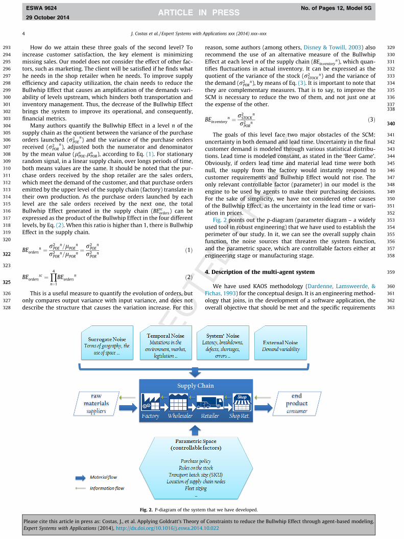
This is a useful measure to quantify the evolution of orders, butonly compares output variance with input variance, and does notdescribe the structure that causes the variation increase. For this
Fig. 2. P-diagram of the system
Please cite this article in press as: Costas, J., et al. Applying Goldratt’s Theory oExpert Systems with Applications (2014), http://dx.doi.org/10.1016/j.eswa.2014.
reason, some authors (among others, Disney & Towill, 2003) alsorecommend the use of an alternative measure of the BullwhipEffect at each level n of the supply chain (BEinventory
n), which quan-tifies fluctuations in actual inventory. It can be expressed as thequotient of the variance of the stock (r2
STOCKn) and the variance of
the demand (r2POR
n), by means of Eq. (3). It is important to note thatthey are complementary measures. That is to say, to improve theSCM is necessary to reduce the two of them, and not just one atthe expense of the other.
BEinventoryn ¼ r2
STOCKn
r2POR
nð3Þ
The goals of this level face two major obstacles of the SCM:uncertainty in both demand and lead time. Uncertainty in the finalcustomer demand is modeled through various statistical distribu-tions. Lead time is modeled constant, as stated in the ‘Beer Game’.Obviously, if orders lead time and material lead time were bothnull, the supply from the factory would instantly respond tocustomer requirements and Bullwhip Effect would not rise. Theonly relevant controllable factor (parameter) in our model is theengine to be used by agents to make their purchasing decisions.For the sake of simplicity, we have not considered other causesof the Bullwhip Effect, as the uncertainty in the lead time or vari-ation in prices.
Fig. 2 points out the p-diagram (parameter diagram – a widelyused tool in robust engineering) that we have used to establish theperimeter of our study. In it, we can see the overall supply chainfunction, the noise sources that threaten the system function,and the parametric space, which are controllable factors either atengineering stage or manufacturing stage.
4. Description of the multi-agent system
We have used KAOS methodology (Dardenne, Lamsweerde, &Fichas, 1993) for the conceptual design. It is an engineering method-ology that joins, in the development of a software application, theoverall objective that should be met and the specific requirements
that we have developed.
f Constraints to reduce the Bullwhip Effect through agent-based modeling.10.022
364
365
366
367
368
369
370
371
372
373
374
375
376
377
378
379
380
381
382
383
384
385
386
387
388
389
390
391
392
393
394
395
396
397
398
399
400
401
402
403
404
405
406
407
408
409
410
411
412
413
414
415
416
417
418
419
420
421
422
423
424
425
426
427
428
429
430
431
432
433
434
435
436
437
J. Costas et al. / Expert Systems with Applications xxx (2014) xxx–xxx 5
ESWA 9624 No. of Pages 12, Model 5G
29 October 2014
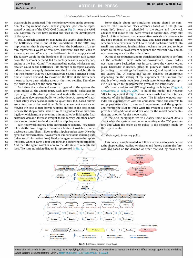
that should be considered. This methodology relies on the construc-tion of a requirement model, whose graphical part can be repre-sented by means of the KAOS Goal Diagram. Fig. 3 shows the KAOSGoal Diagram that we have created and used in the developmentof the system.
TOC approach consists on managing the supply chain based onthe bottleneck. This is one of the foundations of the TOC: anyimprovement that is deployed away from the bottleneck of a sys-tem represents a waste of resources. Therefore, this fact leads toa new question: Where is the bottleneck in this supply chain?The factory would be the bottleneck if its production rate cannotcover the customer demand. But the factory has not a capacity con-straint in the ‘Beer Game’. The intermediate nodes, wholesaler andretailer, could be the bottleneck if its storage or transport capacitydid not allow the supply chain to meet the final demand, but this isnot the situation that we have considered. So, the bottleneck is thefinal customer demand. To maximize the flow at the bottleneckmeans to have zero missing sales at the shop retailer. Therefore,the drum is placed at the shop retailer.
Each time that a demand event is triggered to the system, thedrum makes all the agents react. Each agent (node) calculates itsrope length to the drum position and makes the order decisionbased on its downstream buffer to the bottleneck. Instead of tradi-tional safety stock based on material quantities, TOC-based buffersare a function of the lead time. Buffer management consists onmoving the flow so that arrival happens on time at the bottleneck.Because the shop retailer is the drum, this agent looks for maximiz-ing flow; which means preventing missing sales by linking the finalcustomer demand forecast straight to the factory. All other nodeswork subordinated to the drum with a shipping rope.
Each node works using a finite state machine schema. The agent isidle until the drum triggers it. From the idle state it switches to servebackorders state. Then, it flows to the shipping orders state. Once theagent has moved material downstream, it moves to the sourcing state(take care of information flow). Finally the agent moves to the report-ing state, when it cares about updating and exporting information.And then the agent switches now to the idle state to reiterate theloop. The state transition diagram is represented in Fig. 4.
Fig. 3. KAOS goal diag
Please cite this article in press as: Costas, J., et al. Applying Goldratt’s Theory oExpert Systems with Applications (2014), http://dx.doi.org/10.1016/j.eswa.2014.
Some details about our simulation engine should be com-mented. The simulation clock advances based on a FEL (futureevent list). Events are scheduled in the future and the clockadvance will move to the event which is sooner due. Every takt(block of time between two consecutive arrivals of customers tothe shop retailer) schedules the next one. Each customer arrivalschedules new events in the FEL so to divide each time bucket intosmall time windows. Synchronizing mechanisms are used to forcenodes to follow a downstream sequence for material flow and anupstream sequence for the orders flow.
During these sequences agents transition their states to performall the activities: move material downstream, move ordersupstream, serve backorders just in case, serve the current order,place backorder if needed, place its purchase order upstream(according to the settings for the order policy), and report data intothe export file. Of course the system behaves polymorphousdepending on the setting of the experiment. This means thatdetails of what each node does at each state follows the appropri-ate rules linked to the parameters given at the setup stage.
We have used robust SW engineering techniques (Taguchi,Chowdhury, & Taguchi, 2000) to build the model and NetLogo5.0.5 to implement it. Fig. 5 shows a screenshot of the interfacewindow of the implemented model. The interface window pro-vides the experimenter with the animation frame, the controls tosetup parameters and to run each experiment, and the graphicsand monitoring stuff to track what the system is doing. NetLogoprovides two additional windows, one for the model documenta-tion and another for the model code.
In the next paragraphs we will clarify some relevant detailsabout what the system does when operating under TOC parame-ters and when the order-up-to policy is the selection made bythe experimenter.
4.1. Order-up-to inventory policy
This policy is implemented as follows: at the end of each periodt, the shop retailer, retailer, wholesaler and factory update the fore-cast (bDt) based on the demand or order received, by means of a
ram of our MAS.
f Constraints to reduce the Bullwhip Effect through agent-based modeling.10.022

438
439
440
441
442
443
444
445
446
447
448
449
450
451
452 Q4
453
455455
456
458458
459
461461
462
463
464
465
466
467
468
469
470
471
472
473
474
475
476
477
478
479
480
Fig. 4. State transition diagram (local for each agent).
6 J. Costas et al. / Expert Systems with Applications xxx (2014) xxx–xxx
ESWA 9624 No. of Pages 12, Model 5G
29 October 2014
moving average of the last three observations (Dt-i), according toEq. (4). In this policy, under the assumption of normal demand,the order-up-to point (yt) is estimated as the product of the fore-cast and the lead time (L), plus a term related to the safety stock(Eq. (5)). It depends on a parameter (Z) that is a function of thesecurity level and the standard deviation of the error (St). We haveused Z = 1.64 in order to work with a confidence level of 95%. Thepurchase order quantity for each period is the difference betweenthe order-up-to point of this period and the previous one, plus thedemand of the previous period, by Eq. (6). Note that the purchaseorder arrives at the start of period t + L and sales orders are filled atthe end of each period. More information about this managementpolicy can be found in Chen, Drezner, Ryan, and Simchi-Levi(2001). In our case, we have used a three period moving averageto calculate the forecast.
Fig. 5. Screenshot of the system interface at o
Please cite this article in press as: Costas, J., et al. Applying Goldratt’s Theory oExpert Systems with Applications (2014), http://dx.doi.org/10.1016/j.eswa.2014.
bDt ¼1n�Xn
i¼1
Dt�i ð4Þ
yt ¼ L � bDt þ Z �ffiffiffiLp� St
¼ L � bDt þ Z �ffiffiffiLp�
ffiffiffiffiffiffiffiffiffiffiffiffiffiffiffiffiffiffiffiffiffiffiffiffiffiffiffiffiffiffiffiffiffiffiffiffiffiffiffiffiffiffiffiffi1n�Xn
i¼1
Dt�i �dDt�i
� �2
vuut ð5Þ
qt ¼ yt � yt�1 þ Dt�1
¼ 1þ Ln
� �� Dt�1 �
Ln
� �� Dt�ðnþ1Þ þ Z �
ffiffiffiLp� ðSt � St�1Þ ð6Þ
4.2. DBR methodology – Goldratt’s TOC policy
The DBR methodology has been implemented according tothe Goldratt’s TOC, summarized in Section 2 and following to themeta-model explained above. We should remember that, in thecontext we are considering, the shop retailer is the constraint inthe system, so it must be the drum. The aim of the solution is toprotect it, and therefore the supply chain as a whole, against pro-cess dependency and variation, and thus to optimize the system.In these circumstances, the other levels must be subordinated tothe shop retailer. The buffer is the material release duration andthe rope is the release timing. Youngman (2009) has developedan outstanding guide for the implementation of the TOC in systemsof very different kinds, which can be consulted to get further detailin the process described below.
In the TOC mode, the system operates in two stages. In the firstone, the systemic condition to tie the different levels of the supplychain through time (and not by product) is established. It is theplanning stage and it is orientated to operate the system as awhole. In the second one, the buffer is administered along the
ne particular moment of the simulation.
f Constraints to reduce the Bullwhip Effect through agent-based modeling.10.022
481
482
483
484
485
486
487
488
489
490
491
492
493
494
495
496
497
498
499
500
501
502
503
504
505
506
507
508
509
510
511
512
513
514
515
516
517
518
519
520
521
522
523524526526
527
528
529
530
531
532
533
534
535
536
537
538
539
540
541
542
543
544
545
546
547
548
549
550
551
552
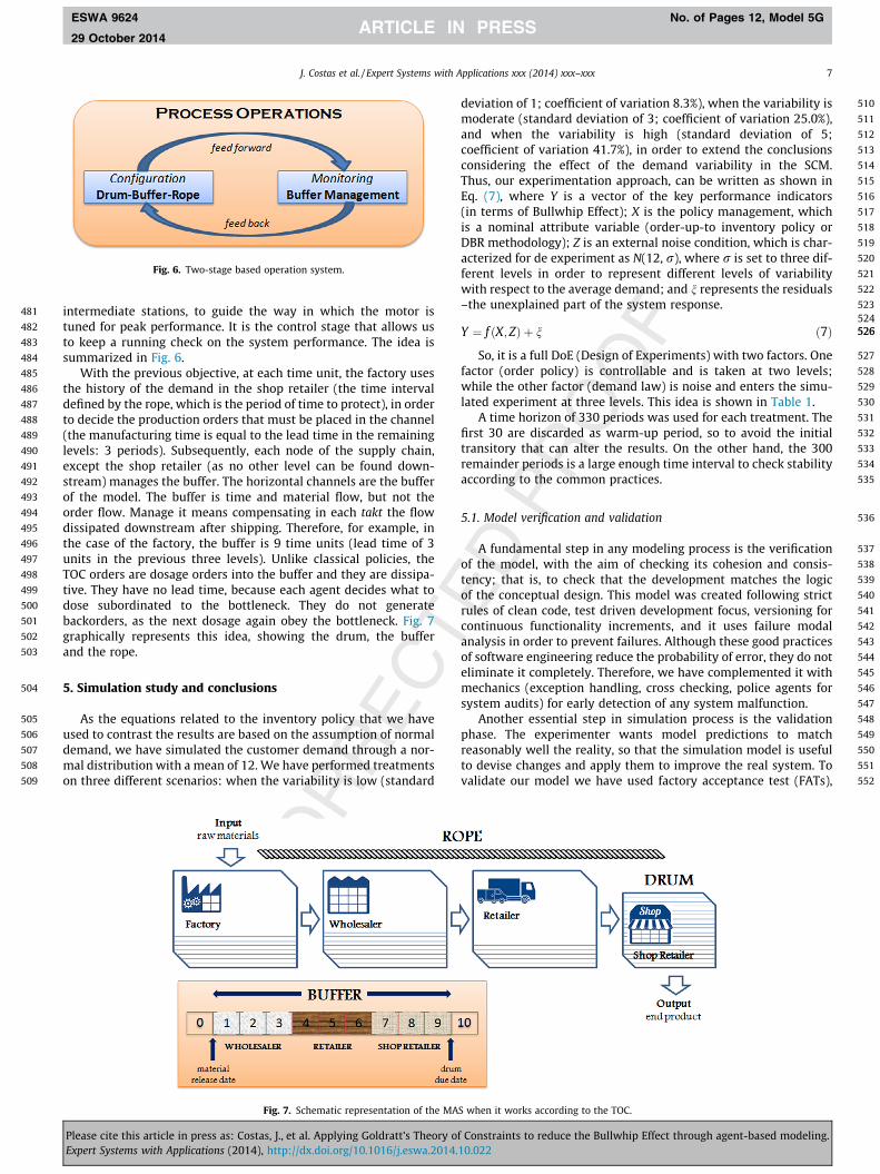
Fig. 6. Two-stage based operation system.
J. Costas et al. / Expert Systems with Applications xxx (2014) xxx–xxx 7
ESWA 9624 No. of Pages 12, Model 5G
29 October 2014
intermediate stations, to guide the way in which the motor istuned for peak performance. It is the control stage that allows usto keep a running check on the system performance. The idea issummarized in Fig. 6.
With the previous objective, at each time unit, the factory usesthe history of the demand in the shop retailer (the time intervaldefined by the rope, which is the period of time to protect), in orderto decide the production orders that must be placed in the channel(the manufacturing time is equal to the lead time in the remaininglevels: 3 periods). Subsequently, each node of the supply chain,except the shop retailer (as no other level can be found down-stream) manages the buffer. The horizontal channels are the bufferof the model. The buffer is time and material flow, but not theorder flow. Manage it means compensating in each takt the flowdissipated downstream after shipping. Therefore, for example, inthe case of the factory, the buffer is 9 time units (lead time of 3units in the previous three levels). Unlike classical policies, theTOC orders are dosage orders into the buffer and they are dissipa-tive. They have no lead time, because each agent decides what todose subordinated to the bottleneck. They do not generatebackorders, as the next dosage again obey the bottleneck. Fig. 7graphically represents this idea, showing the drum, the bufferand the rope.
5. Simulation study and conclusions
As the equations related to the inventory policy that we haveused to contrast the results are based on the assumption of normaldemand, we have simulated the customer demand through a nor-mal distribution with a mean of 12. We have performed treatmentson three different scenarios: when the variability is low (standard
Fig. 7. Schematic representation of the MA
Please cite this article in press as: Costas, J., et al. Applying Goldratt’s Theory oExpert Systems with Applications (2014), http://dx.doi.org/10.1016/j.eswa.2014.
deviation of 1; coefficient of variation 8.3%), when the variability ismoderate (standard deviation of 3; coefficient of variation 25.0%),and when the variability is high (standard deviation of 5;coefficient of variation 41.7%), in order to extend the conclusionsconsidering the effect of the demand variability in the SCM.Thus, our experimentation approach, can be written as shown inEq. (7), where Y is a vector of the key performance indicators(in terms of Bullwhip Effect); X is the policy management, whichis a nominal attribute variable (order-up-to inventory policy orDBR methodology); Z is an external noise condition, which is char-acterized for de experiment as N(12, r), where r is set to three dif-ferent levels in order to represent different levels of variabilitywith respect to the average demand; and n represents the residuals–the unexplained part of the system response.
Y ¼ f ðX; ZÞ þ n ð7Þ
So, it is a full DoE (Design of Experiments) with two factors. Onefactor (order policy) is controllable and is taken at two levels;while the other factor (demand law) is noise and enters the simu-lated experiment at three levels. This idea is shown in Table 1.
A time horizon of 330 periods was used for each treatment. Thefirst 30 are discarded as warm-up period, so to avoid the initialtransitory that can alter the results. On the other hand, the 300remainder periods is a large enough time interval to check stabilityaccording to the common practices.
5.1. Model verification and validation
A fundamental step in any modeling process is the verificationof the model, with the aim of checking its cohesion and consis-tency; that is, to check that the development matches the logicof the conceptual design. This model was created following strictrules of clean code, test driven development focus, versioning forcontinuous functionality increments, and it uses failure modalanalysis in order to prevent failures. Although these good practicesof software engineering reduce the probability of error, they do noteliminate it completely. Therefore, we have complemented it withmechanics (exception handling, cross checking, police agents forsystem audits) for early detection of any system malfunction.
Another essential step in simulation process is the validationphase. The experimenter wants model predictions to matchreasonably well the reality, so that the simulation model is usefulto devise changes and apply them to improve the real system. Tovalidate our model we have used factory acceptance test (FATs),
S when it works according to the TOC.
f Constraints to reduce the Bullwhip Effect through agent-based modeling.10.022
553
554
555
556
557
558
559
560
561
562
563
564
565
566
567
568
569
570
571
572
573
574
575
576
577
578
579
580
581
582
583
584
585
586
587
588
589
590
591
592
593
594
595
596
597
Table 1DoE (Design of Experiments) table.
Factor Level Treatment Demand law (Z) Order policy (X)
Demand law Normal(12,1) 1 Normal (12,1) Order-up-to inv. pol.(Z) Normal(12,3) 2 Normal (12,3) Order-up-to inv. pol.
Normal(12,5) 3 Normal (12,5) Order-up-to inv. pol.4 Normal (12,1) DBR methodology
Order policy Order-up-to inv. pol. 5 Normal (12,3) DBR methodology(X) DBR methodology 6 Normal (12,5) DBR methodology
Q6
8 J. Costas et al. / Expert Systems with Applications xxx (2014) xxx–xxx
ESWA 9624 No. of Pages 12, Model 5G
29 October 2014
so to confirm that the model exhibits a well known behavior whenexposed to controlled conditions. As an example, we include onethis kind of tests that are implemented in the model.
5.1.1. Test conditions
(I) Constant demand in the shop retailer: 12 sku/period.(II) Damaged equipment on the factory: zero production.
5.1.2. Expected behavior
(I) It only serves customers until the initial stock is depleted.(II) Cumulative backorders are generated at each node.
5.1.3. Acceptance criteria
(I) Demand turns into missing sales (12 sku/period) in steadystate.
(II) Storage costs are zero in steady state.
Once the FAT tests were satisfactory, the standard approach wasused when comparing treatments under stochastic conditions:each treatment is replicated (it was run three times) so that thestatistical analysis takes into account the experimental error. An
Table 2Results of the tests when the order-up-to inventory policy is used (I): mean (left) and varianin the different levels of the supply chain (without warm-up time).
Process metrics Scenario 1 lowvariability [treatment 1]
Consumer demand 11.98–1.04Shop retailer purchase orders 11.47–98.39Retailer purchase orders 12.04–380.20Wholesaler purchase orders 11.79–1405.58Factory production 12.08–4247.31Shop retailer inventory 12.0–101.1Retailer inventory 67.9–1011.38Wholesaler inventory 218.9–13471.1Factory inventory 577.7–32599.2
Table 3Results of the tests when the order-up-to inventory policy is used (II): Orders Bullwhip Efmissing sales to evaluate the performance of the supply chain (without warm-up time).
Performance Metrics Scenario 1 lowvariability [treatment 1]
Shop retailer bullwhip effect [orders] 99.13Retailer bullwhip effect [orders] 3.68Wholesaler bullwhip effect [orders] 3.78Factory bullwhip effect [orders] 2.95Supply chain bullwhip effect [orders] 4063.14Shop retailer missing sales [sku] 163Shop retailer bullwhip effect [inventory] 97.58Retailer bullwhip effect [inventory] 10.28Wholesaler bullwhip effect [inventory] 35.43Factory bullwhip effect [inventory] 23.19
Please cite this article in press as: Costas, J., et al. Applying Goldratt’s Theory oExpert Systems with Applications (2014), http://dx.doi.org/10.1016/j.eswa.2014.
overall stability study (run several trajectories –replicas– of eachexperimental treatment) about the key output metrics (lost sales,stocks) was also conducted. And, of course, we did care about theexperimental error (using replicas and hypothesis testing).
The model statistically probed to be valid: matched expectedoutputs under controlled scenarios, reached stability and haverepeatability.
5.2. Analysis of the treatments
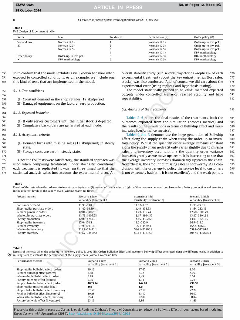
Tables 2–5 report the final results of the treatments, both theoutcomes exported from the simulation (process metrics) andthe results of the simulations in terms of Bullwhip Effect and miss-ing sales (performance metrics).
Tables 2 and 3 demonstrate the huge generation of BullwhipEffect along the supply chain when using the order-up-to inven-tory policy. Whilst the quantity order average remains constantalong the supply chain nodes (it only varies slightly due to missingsales and inventory accumulation), the quantity order varianceincreases greatly as we move upstream. It is interesting to see thatthe average inventory increases dramatically upstream the chain.Nevertheless, the amount of missing sales is noteworthy. As a con-clusion, with the order-up-to policy the service level to customersis not extremely bad (still, it is not excellent), and the weak point is
ce (right) of the consumer demand, purchase orders, factory production and inventory
Scenario 2 midvariability [treatment 2]
Scenario 3 highvariability [treatment 3]
11.97–7.97 11.91–27.6111.49–133.53 11.64–232.1311.79–715.74 12.50–1008.7913.17–1994.30 13.47–3304.9414.15–4162.65 13.03–7228.6619.2–215.9 34.9–613.6105.1–4429.3 154.5–8362.3384.1–22900.2 559.9–51286.0593.1–13674.0 1057.0–137635.3
fect and Inventory Bullwhip Effect generated along the different levels, in addition to
Scenario 2 midvariability [treatment 2]
Scenario 3 highvariability [treatment 3]
17,47 8.605,22 4.052,49 3.041,94 2.26442.07 239.33124 8627,10 22.2233,17 36.0232,00 50.846,86 41.65
f Constraints to reduce the Bullwhip Effect through agent-based modeling.10.022

598
599
600
601
602
603
604
605
606
607
608
609
610
611
612
613
614
615
616
617
618
619
620
621
622
623
624
625
626
627
628
629
630
631
632
633
634
635
636
637
638
639
640
641
642
643
644
645
646
647
648
649
650
651
652
653
654
655
656
657
658
659
660
661
662
663
664
665
Table 4Results of the tests when the DBR methodology is used (I): Mean (left) and variance (right) of the consumer demand, purchase orders, factory production and inventory in thedifferent levels of the supply chain (without warm-up time).
Process metrics Scenario 1 lowvariability [treatment 4]
Scenario 2 midvariability [treatment 5]
Scenario 3 highvariability [treatment 6]
Consumer demand 12.07–1.13 12.47–11.03 11.79–24.43Shop retailer purchase orders 12.10–9.11 13.04–75.82 12.83–134.10Retailer purchase orders 12.10–7.32 12.33–58.37 11.66–101.48Wholesaler purchase orders 12.09–5.63 12.36–53.60 11.47–110.75Factory production 12.09–7.98 12.47–76.48 11.39–145.03Shop retailer inventory 9.2–12.5 16.8–74.1 21.9–142.9Retailer inventory 14.0–23.8 18.6–140.4 20.6–209.7Wholesaler inventory 50.7–17.2 56.5–190.7 59.3–523.7Factory inventory 97.1–18.0 113.6–162.0 121.0–441.1
Table 5Results of the tests when the DBR methodology is used (II): Bullwhip Effect and Alternative Bullwhip Effect generated along the different levels, missing sales and Goldratt’soperational metrics to evaluate the performance of the supply chain (without warm-up time).Q7
Performance metrics Scenario 1 low variability [treatment 4] Scenario 2 mid variability [treatment 5] Scenario 3 high variability [treatment 6]
Shop retailer bullwhip effect [orders] 8.02 6.57 5.05Retailer bullwhip effect [orders] 0.80 0.81 0.83Wholesaler bullwhip effect [orders] 0.77 0.92 1.11Factory bullwhip effect [orders] 1.42 1.42 1.32Supply chain bullwhip effect [orders] 7.03 6.94 6.15Shop retailer missing sales [sku] 1 54 82Shop retailer bullwhip effect [inventory] 11.01 6.72 5.85Retailer bullwhip effect [inventory] 2.61 1.85 1.56Wholesaler bullwhip effect [inventory] 2.34 3.27 5.16Factory bullwhip effect [inventory] 3.19 3.02 3.98
J. Costas et al. / Expert Systems with Applications xxx (2014) xxx–xxx 9
ESWA 9624 No. of Pages 12, Model 5G
29 October 2014
that this bad service is obtained at a huge cost in terms of inven-tory. The lesson learnt, and it is very usual in the marketplace, isthat the customer service is protected with huge inventory and thispolicy is not effective, because the root cause of the problems is notbeing considered. According to the industrial experience of theauthors, this is a very common finding in ailing processes.
Looking at these tables, it can be seen that the greatest BullwhipEffect is generated, according to the classical formulation, in thescenario of low variability. Obviously, the greater the variabilityin consumer demand, the greater the variability in the rate of pro-duction of the factory. However, the relationship between the twovariances is much larger when the variability in consumer demandis low. Moreover, this classic inventory management policy gener-ates more missing sales when the variability of consumer demandis low. At first glance, this result might seem surprising, but it isnot, as the explanation lies in the level of inventories: when thevariability is very high, the levels of the supply chain tend to beoverprotective. For this reason, the missing sales are reduced atthe expense of increasing the inventory far from the customer.
Tables 4 and 5 point out that the TOC also causes BullwhipEffect in the supply system, since variability in purchase ordersincreases and both the mean and the variance of the inventorylevel increment as they move away from the consumer. However,a simple comparison of these tables with respect to Tables 1 and 2makes clear the enormous effectiveness of DBR methodology inmanaging the supply chain. The amplification of the variability oforders is much lower when the supply chain is managed accordingto the practices proposed by Goldratt. Likewise, the TOC gets tomanage the supply chain with minor inventories at all levels.Moreover, despite that, the amount of missing sales decreasesmeaningfully. Hence, the important findings using TOC approachis that both negative effects (Bullwhip Effect and missing sales)reduce at the same time when compared to the order-up-to policy.
The generation of the Bullwhip Effect in the supply chain and theimprovements introduced by Goldratt’s practices in comparison
Please cite this article in press as: Costas, J., et al. Applying Goldratt’s Theory oExpert Systems with Applications (2014), http://dx.doi.org/10.1016/j.eswa.2014.
with the traditional management policies can be shown graphicallyin many different ways. For example, Fig. 8 exhibits the productionrate of the factory throughout the time horizon for the two testsassuming normal with mean 12 and standard deviation 3 in thefinal consumer. When the system works according to the order-up-to inventory policy, the factory production varies greatly: inmost periods, it has no production needs while in some specificmoments it must manufacture very high amounts of product. Withthe DBR methodology, however, variability in the factory produc-tion is much lower, which translates in cost savings from differentperspective (among others, labor, inventory, and transportationcosts).
Why does such amplification occur? When the supply chain ismanaged according to the order-up-to inventory policy, the peaksin orders received for each level translate into an even bigger peakin orders placed by that level. The time difference is the lead time.That is to say, each level contributes increasing the distortion inthe supply chain, and so decreasing the reliability of the transmit-ted information. When using TOC, the supply chain performsdramatically better.
The other way to observe the Bullwhip Effect is through theinventory of the various levels. It is possible to see it, for example,by means of box plots. Fig. 9 shows these graphs, with the average,the indicators of the first and third quartile and the upper andlower limits, for the stock of the different members of the supplychain in tests with mean 12 and standard deviation 5. It shouldbe noted that the values lower than 0 are related to inventorybackorders that will be met the following periods. It is enough tocompare the vertical scale of the two graphs to observe theimprovements introduced by TOC, both in mean and in variance.
5.3. Statistical significance of results
By looking at the plots shown above we have visual evidencethat the supply chain performs much better when using TOC, as
f Constraints to reduce the Bullwhip Effect through agent-based modeling.10.022

666
667
668
669
670
671
672
673
674
675
676
677
678
679
680
681
682
683
684
685
686
687
688
689
690
691
692
693
694
695
696
697
698
699
700
701
702
703
704
705
706
707
708
709
710
711
712
713
714
715
716
Fig. 8. Factory production in the two tests (order-up-to inventory policy and DBR methodology) carried out with a N(12,3).
Fig. 9. Box plots of the inventory level in the different members of the supply chain in the two tests (order-up-to inventory policy and DBR methodology) carried out with aN(12,5).
10 J. Costas et al. / Expert Systems with Applications xxx (2014) xxx–xxx
ESWA 9624 No. of Pages 12, Model 5G
29 October 2014
commented. Nevertheless, it should be formally verified. The sta-tistical tests were conducted for the different treatments, althoughthey are only shown in one case, by way of example.
First, we concentrate on missing sales at the shop retailer,which is the only point where the fact of missing sales is really acritical concern. When the standard deviation of the demand is 5,we have the distribution for the missing sales penalty in each timebucket (sample size N > 150, once excluded the warm-up period).We have tested the null hypothesis ‘‘H0: missing sales mean = 0’’.For the order-up-to inventory policy, using 1-sample t test has apValue less than 5%, which rejects null hypothesis. So, the penaltyfor missing sales is significantly different from zero. On the otherhand, running a same length trajectory with TOC, all time buckets,after the warm-up period, have zero lost sales. The conclusion isthat TOC policy effectively protects the supply chain against losingsales, whilst this does not happen with the order-up-to policy.
Once we have got formal evidence that the supply chainperformance significantly improves when applying TOC in termsof external customer satisfaction (here, maximizing sales byexploiting the bottleneck), we now take care of getting also formalevidence that this achievement is not at the expense of increasinginventory cost in the overall supply chain. The inventory total costhas been collected during a long (for example, 200 time buckets)period of time after the system warm-up, and proceed first tocheck is the variance of this metric is unequal when using TOC ver-sus when using order-up-to policy. We check, using a 2-variancetest, the null hypothesis ‘‘H0: variance (total inventory cost in the
Please cite this article in press as: Costas, J., et al. Applying Goldratt’s Theory oExpert Systems with Applications (2014), http://dx.doi.org/10.1016/j.eswa.2014.
supply chain)|policy = TOC) = variance (total inventory cost in the sup-ply chain)|policy = order-up-to)’’. Fig. 10 shows that in the sample,the standard deviation statistic of the metric at TOC level is lessthan at order-up-to level; the Levene test shows a p-value lowerthan 5%; so we reject null hypothesis. Therefore, TOC policyinduces less variance in the inventory cost (so, to the goal stockin the system).
Fig. 10 also displays the Welch’s test to compare the means.Again, we reject the null hypothesis ‘‘H0: mean (total inventory costin the supply chain)|policy = TOC) = mean (total inventory cost in thesupply chain)|policy = order-up-to)’’. And, we take the alternativehypothesis: the total inventory cost in the supply chain is lesswhen we use TOC policy. In conclusion, as expected, TOC not onlygives a full protection against missing sales (while order-up-todoes not), but besides, TOC achieve this result even reducing thetotal inventory cost (less variance and lower mean).
6. Findings, recommendations and next steps
The new competitive environment has granted the SupplyChain Management a strategic role in the search for competitiveadvantage. For this reason, the orders variance amplification alongthe supply chain, known as the Bullwhip Effect, is an importantconcern for businesses, as it is a major cause of inefficiencies.Traditional management policies linked to the mass productionparadigm, such as order-up-to inventory policy, are unsuccessful
f Constraints to reduce the Bullwhip Effect through agent-based modeling.10.022

717
718
719
720
721
722
723
724
725
726
727
728
729
730
731
732
733
734
735
736
737
738
739
740
741
742
743
744
745
746
747
748
749
750
751
752
753
754
755
756
757
758
759
760
761
762
763
764
765
766
767
768
769
770
771
772
773
774
775
776
777
778
779
780
781Q5
782
783
784
785
786
787
788
789790791792793794795796797798799
Fig. 10. Hypothesis contrast to the significant difference between the inventory costs and averages of both policies.
J. Costas et al. / Expert Systems with Applications xxx (2014) xxx–xxx 11
ESWA 9624 No. of Pages 12, Model 5G
29 October 2014
–as already shown in literature– in terms of fighting the BullwhipEffect.
KAOS methodology was used to devise the multi-agent simula-tion model carried out on this research. The Gall’s incrementalprinciple (a complex system that works properly has evolved froma simple system which was effective) has been applied to end upwith a highly reliable, self-controlled, tested and flexible modelso to experiment TOC approach versus order-up-to policies formanaging a multi-echelon supply chain and collect data evidenceof system behavior. Statistical analysis have been applied to thesedata blocks taking into account the warm-up period, stability studyand the final hypothesis testing to raise our conclusions.
Our first finding was that the higher the final customer demandvariability, the higher is the amplification upstream the supplychain, because each node tends to overprotect itself due to the fearof breaking stock.
TOC philosophy has demonstrated in this work that is highlyeffective in remedying this issue. A dramatic improvement in theoverall supply chain has been reached in several explored levelsof external demand variability, but the more important point isthat every level has improved its own performance by subordinat-ing to the bottleneck. Hence, the best solution for the system is thebest solution for each individual member.
The major contribution of this work has been to demonstratethat considering only the main effects, there are enough reasonsto manage the supply chain according to Goldratt’s philosophy.
There are plenty of model extensions and future works that thisresearch group is planning as next steps on this fascinating topic.
(1) To analyze why, provided that TOC is a mature and validatedtheory, it is not yet widely used. We wonder that moving theagents away from their natural egoist behavior needs someeducational phases, and simulation can play an importantrole here.
(2) To extend this model to a larger noise conditions scenario.Now the noise factors have been limited in the model toinclude only different levels of variability in the externaldemand and to keep constant the delays in the materialand in the information flows. Of course, considering otherdisturbance factors like scrap, variability in transportationdelays, errors in the information flow and other sources ofwaste in the supply chain, a comparison of system robust-ness using TOC versus other management policies canprovide insights to other relevant findings.
Please cite this article in press as: Costas, J., et al. Applying Goldratt’s Theory oExpert Systems with Applications (2014), http://dx.doi.org/10.1016/j.eswa.2014.
(3) To place SCM rules and controls to prevent selfish behaviorof agents that could operate against the supply chain majorinterests. We also plan to explore to what extent agentsapplying fuzzy logic decision in their quest of local optimacompares against applying holistic fuzzy logic decision mak-ing engines. Thereby, the concept of the Nash Equilibrium insupply chains must be introduced.
(4) To model adaptive mechanisms on the supply chain in orderto detect and react to bottleneck displacements; forinstance, due to changes in the storage technology, storagepolicies, multimodal transportations costs and so forth.
Even though the shift in our production and managementsystems was initiated after World War II, with lean manufacturingtaking over the mass production paradigm, the systemic approachhas spread in a very irregular way. Agent-based modeling andsimulation is an important tool to educate people, and to contrib-ute to create critical mass for a large deployment of the systemicapproach, which in the end translates in a better skilled populationto deal with complex systems like supply chains.
7. Uncited reference
Wilensky (1999).
Acknowledgements
The authors deeply appreciate the financial support provided bythe Government of the Principality of Asturias, through the ‘SeveroOchoa’ program (reference BP13011). We would also like to thankProfessor Isabel Fernández for making a valuable contribution tothe discussion and for her interesting comments.
References
Andel, T. (1996). Manage inventory, own information. Transportation & Distribution,37(5), 54–58.
Buchmeister, B., Friscic, D., Lalic, B., & Palcic, I. (2012). Analysis of a three-stagesupply chain with level constraints. International Journal of Simulation Modelling,11(4), 196–210.
Chatfield, D. C., & Pritchard, A. M. (2013). Returns and the bullwhip effect.Transportation Research Part E: Logistics and Transportation Review, 49(1),159–175.
Chen, F., Drezner, Z., Ryan, J. K., & Simchi-Levi, D. (2001). Quantifying the bullwhipeffect in a simple supply chain: The impact of forecasting, lead times, andinformation. Management Science, 46(3), 436–443.
f Constraints to reduce the Bullwhip Effect through agent-based modeling.10.022

800801802803804805806807808809810811812813814815816817818819820821822823824825826827828829830831832833834835836837838839840841842
843844845846847848849850851852853854855856857858859860861862863864865866867868869870871872873874875876877878879880881882883884885
12 J. Costas et al. / Expert Systems with Applications xxx (2014) xxx–xxx
ESWA 9624 No. of Pages 12, Model 5G
29 October 2014
Chen, L., & Lee, H. L. (2012). Bullwhip effect measurement and its implications.Operations Research, 60(4), 771–784.
Cole, H., & Jacob, D. (2003). Introduction to TOC supply Chain. AGI Institute.Cox, J. F., & Spencer, M. S. (1998). The constraints management handbook. Boca Raton,
FL: Lucie Press.Dardenne, A., Lamsweerde, A., & Fichas, S. (1993). Goal-directed requirements
acquisition. Science of Computer Programming, 20, 3–50.De la Fuente, D., & Lozano, J. (2007). Application of distributed intelligence to reduce
the bullwhip effect. International Journal of Production Research, 44(8),1815–1833.
DesMarteu, K. (1998). New VICS publication provides step-by-step guide to CPFR.Bobbin, 40(3), 10.
Disney, S. M., Farasyn, I., Lambrecht, M., Towill, D. R., & Van de Velde, W. (2005).Taming the bullwhip effect whilst watching customer service in a single supplychain echelon. European Journal of Operational Research, 173(1), 151–172.
Disney, S. M., & Towill, D. R. (2003). On the bullwhip and inventory varianceproduced by an ordering policy. Omega – The International Journal onManagement Science., 31, 157–167.
Forrester, J. W. (1961). Industrial dynamics. Cambridge, MA: MIT Press.Fox, M. S., Chionglo, J. F., & Barbuceanu, M. (1993). The integrated supply chain
management system. Internal Report, Dept. of Industrial Engineering,University of Toronto.
Goldratt, E. M. (1990). Theory of constraints. Croton-on-Hudson, NY: North RiverPress.
Goldratt, E. M. (1994). It’s not luck. Great Barrington, MA: North River Press.Goldratt, E. M. (1997). Critical chain. Great Barrington, MA: North River Press.Goldratt, E. M., & Cox, J. (1984). The goal – A process of ongoing improvement. Croton-
on-Hudson, NY: North River Press.Goldratt, E. M., Schragenheim, E., & Ptak, C. A. (2000). Necessary but not sufficient.
Croton-on-Hudson, NY: North River Press.Kaminsky, P., & Simchi-Levi, D. (1998). A new computerized beer game: a tool for
teaching the value of integrated supply chain management. In H. Lee & S. M. Ng(Eds.), Supply Chain and Technology Management. Miami, Florida: The Productionand Operations Management Society.
Kimbrough, S. O., Wu, D. J., & Zhong, F. (2002). Computers play the beer game: canartificial manage supply chains? Decision Support Systems, 33, 323–333.
Lee, H. L., Padmanabhan, V., & Whang, S. (1997). The bullwhip effect in supplychains. MIT Sloan Management Review, 38(3), 93–102.
Liang, W. Y., & Huang, C. C. (2006). Agent-based demand forecast in multi-echelonsupply chain. Decision Support Systems, 42(1), 390–407.
Mangina, E., & Vlachos, I. P. (2005). The changing role of information technology infood and beverage logistics management: Beverage network optimization usingintelligent agent technology. Journal of Food Engineering, 70(3), 403–420.
886
Please cite this article in press as: Costas, J., et al. Applying Goldratt’s Theory oExpert Systems with Applications (2014), http://dx.doi.org/10.1016/j.eswa.2014.
Maturana, F., Shen, W., & Norrie, D. H. (1999). MetaMorph: An adaptive agent-basedarchitecture for intelligent manufacturing. International Journal of ProductionResearch, 37(10), 2159–2173.
McKinsey, J. (1992). Evaluating the impact of alternative store formats. SupermarketIndustry Convention. Chicago: Food Marketing Institute.
Saberi, S., Nookabadi, A. S., & Hejazi, S. R. (2012). Applying agent-based system andnegotiation mechanism in improvement of inventory management andcustomer order fulfillment in multi echelon supply chain. Arabian Journal forScience and Engineering, 37(3), 851–861.
Schweitzer, F., Fagiolo, G., Sornette, D., Vega-Redondo, F., Vespignani, A., & White, D.R. (2009). Economic networks: The new challenges. Science, 325(5939),422–425.
Simatupang, T. M., Hurley, S. F., & Evans, A. N. (1997). Revitalizing TQM efforts: aself-reflection diagnosis based on the theory of constraints. ManagementDecision, 35(10), 746–752.
Simatupang, T. M., Wright, A. C., & Sridharan, R. (2004). Applying the theory ofconstraints to supply chain collaboration. Supply Chain Management: AnInternational Journal, 9(1), 57–70.
Sterman, J. D. (1989). Modeling managerial behavior: Misperceptions of feedback ina dynamic decision making experiment. Management Science, 35(3), 321–339.
Taguchi, G., Chowdhury, S., & Taguchi, S. (2000). Robust engineering. New York: McGraw-Hill.
Umble, M., Umble, E., & von Deylen, L. (2001). Integrating enterprise resourcesplanning and theory of constraints: A case study. Production and InventoryManagement Journal, 42(2), 43–48.
Wilensky, U. (1999). NetLogo. Northwestern University, Evanston, IL: The Center forConnected Learning and Computer – Based Modeling. <http://ccl.northwestern.edu/netlogo/>. Last access 10 April 2014.
Wooldridge, M. (2000). Reasoning about rational agents. Cambridge, Mass: MIT Press.Wu, H. H., Chen, C. P., Tsai, C. H., & Tsai, T. P. (2010). A study of an enhanced
simulation model for TOC supply chain replenishment system under capacityconstraint. Expert Systems with Applications, 37, 6435–6440.
Wu, H. H., Lee, A. H. I., & Tsai, T. P. (2014). A two-level replenishment frequencymodel for TOC supply chain replenishment systems under capacity constraint.Computers & Industrial Engineering, 72, 152–159.
Youngman, K. (2009). A guide to implementing the theory of constraints (TOC).<http://www.dbrmfg.co.nz/>. Last access 9 July 2014.
Yuan, K. J., Chang, S. H., & Li, R. K. (2003). Enhancement of theory of constraintsreplenishment using a novel generic buffer management procedure.International Journal of Production Research, 41(4), 725–740.
Zarandi, M. H., Fazel Pourakbar, M., & Turksen, I. B. (2008). A fuzzy agent-basedmodel for reduction of bullwhip effect in supply chain systems. Expert Systemswith Applications, 34(3), 1680–1691.
f Constraints to reduce the Bullwhip Effect through agent-based modeling.10.022