Expertise inQualitative Prediction

of Behaviour

Ph.D. thesis (Chapter 2)

University of AmsterdamAmsterdam, The Netherlands

1992

Bert Bredeweg

Chapter 2

Approaches to Qualitative

Reasoning

This chapter describes the state of the art of qualitative reasoning in three subsections.

First an introduction to the �eld is given. The purpose of this introduction is to allow the

reader to become familiar with the objectives in this area of arti�cial intelligence. The

second section gives a detailed description of the three main approaches to qualitative

reasoning. The last section discusses the main problems within the area of qualitative

prediction. In this discussion we will concentrate on the problems concerning the three

approaches mentioned before.

2.1 Introduction to the Field

In its most general form qualitative reasoning is concerned with reasoning about the be-

haviour of systems present in the real-world in qualitative terms. Although any system

might be an object of such a reasoning process, the majority of research deals with reason-

ing about physical systems.1 The behavioural aspect studied most is qualitative prediction

of behaviour, i.e. analysing how the behaviour of a system evolves as time passes.

Figure 2.1 shows an intuitive example of what qualitative reasoning encompasses (cf.

[70; 73]). The problem is to predict what will happen to a closed container (a boiler), par-

tially �lled with water, when it is heated by some energy source. The answer a qualitative

reasoner might produce is the following:

1. Because of the energy added by the heat source, both the temperature and the pres-

sure of the water will increase. This behaviour may lead to three other behaviours:

2, 3 or 4.

2. The container explodes because the internal pressure is too high for the container.

The reaction force generated by the container is lower than the pressure exerted by

the substance. The container is broken after this behaviour.

3. The temperature of the water reaches its boiling point and starts boiling. Steam is

generated. This behaviour may lead to three other behaviours: 2, 4 or 5.

1Economics is a good example of a non-physical domain in which qualitative reasoning is used [69; 8].

5

Heater

What happens?

The watertemperatureand pressure

increase

The boilerexplodes, because the

internal substancepressure is too

high

The waterstarts boiling,

steam isgenerated

All the waterhas turned to

steam

The substancetemperature andthe temperature

of the heaterbecome equal

Water

Figure 2.1: Behaviour prediction of a boiler heating water

4. The temperature of the substance in the container (be it water or steam) is now

equal to the temperature of the heat source. From here on, no further changes take

place.

5. All the water has now turned into steam. This behaviour may lead to two other

behaviours: 2 or 4.

This behaviour prediction is not necessarily the only answer to the problem. Speci�c

abstractions have been made to provide an understandable solution. The description does

not, for example, include a state of behaviour in which the water starts boiling and at the

same moment the container explodes, although in principle this combination is possible.

2.1.1 The Objectives

De Kleer and Brown [57] formulate the following three objectives for qualitative reasoning:

� It should be simpler than classical physics and yet retain all the important con-

cepts (e.g. state, oscillation, gain, momentum) without invoking the mathematics of

continuously varying quantities and di�erential equations.

� It should produce causal accounts for physical mechanisms.

� It should provide foundations for common sense models for the next generation of

expert systems.

2.1.1.1 Qualitative Physics

De Kleer [51] illustrates the need for a qualitative physics by pointing out three reasons

why writing down conventional mathematical equations is inappropriate for reasoning

about physics:

6

� a qualitative analysis is crucial for comprehending the problem and writing down

the appropriate equations,

� solving equations is intractable unless they are based on the right idealisation and

approximation of the system that is reasoned about, and

� people do not believe the answers predicted by equations unless these answers can

be supported by an intuitive understanding.

2.1.1.2 Causal Interpretations

Providing causal accounts for the behaviour of physical systems can be illustrated with

the propulsion system [76], which is depicted in �gure 2.2. This device, which is used in

Heater

Superheater

Output

Input

Figure 2.2: The propulsion system

submarines, takes water from the ocean and turns it to steam by heating it with oil-�red

burners. The steam, evaporating from the water surface, leaves the boiler and is heated

for a second time, to impart additional kinetic energy.

An interesting problem to solve about this system, is the following:

� what happens to the temperature of the steam leaving the outlet when the temperature

of the feed-water at the inlet increases?

The answer can only be given by constructing the right causal model of the behaviour

manifested by the propulsion system. Consider, for example, the following interpretation.

The boiling takes place at a constant temperature, which means that although the feed-

water is warmer, it will still turn to steam at the same temperature as the colder feed-water.

However, if the feed-water is warmer it requires less energy to reach its boiling point. If

we assume a constant energy supply by the heat source, we can conclude that more water

will be turned to steam if the temperature of the feed-water increases. As the rate of

the steam production increases, more steam will have to pass the superheater within the

same amount of time. Since the amount of heat transferred depends on the time the

steam spends in the superheater, the steam will leave the outlet with a lower temperature,

because there is less time for the superheater to heat up the steam. So the answer to the

question is that the temperature of the steam at the outlet falls when the temperature of

the water at the inlet increases. A solution like this can only be derived on the basis of a

causal interpretation of the behaviour of the system.

7

2.1.1.3 Pre-physics and Common Sense Knowledge

The notion of common sense models encompasses the idea that the laws formulated in

traditional physics comprise only a small fraction of the, mostly pre-physics, knowledge

that is required for reasoning about a system in the physical world. De Kleer gives some

examples of this type of knowledge when he discusses his experience with the Newton

program [50]. This program was developed for solving problems about the roller coaster

(see �gure 2.3). A typical problem is determining how high the cart should start in order

R

H

Figure 2.3: The roller coaster with a loop-the-loop

to traverse the loop-the-loop without falling of. Faced with this problem students do not

solve it by `simply' applying all kinds of speci�c equations. Instead they have extensive

common sense knowledge about the problem which they use as guidance for focusing on

the relevant aspects of the system. De Kleer points out the following examples:

� How do students know that the cart rolls down, not up, when released?

� How do students know that the cart after building up enough speed, does not fall of

at the top of the loop?

� How do students know that, once the cart starts rolling up the initial section of the

loop, rolling back is a possibility, but not (yet) falling of?

� How do students know that, once the cart travels upside down, it might fall o�, but

not roll back?

The answers to these questions may seem obvious, but it is exactly this pre-physics

knowledge that people are good at, but for which there exists no formalised theory that can

be used for implementing it on computers. It is only after questions like these have been

answered that the analysis of the problem becomes relatively straightforward. The exam-

ple therefore shows that people bring to bear enormous amounts of pre-physics knowledge.

This knowledge is accumulated while growing up in the physical world that surrounds us.

If we want machines, in particular computers, to reason about the physical world, we must

�rst make this knowledge available to them.

8

2.1.2 Qualitative Reasoning and Traditional Physics

There are a number of reasons why traditional physics is limited as a single approach

for reasoning about the behaviour of (physical) systems. Firstly, there are only partial

formal axiomatic theories of physics. De Kleer [51] in this respect points out that it is not

possible to �nd a physics text that tells us how to �gure out when a ball stops bouncing

and starts rolling after it has been thrown onto a carpet. Qualitative reasoning may be

used for developing theories of physics.

A second reason is that there are certain physical research issues which are not posed

as such in traditional physics. In particular, the problem of qualitative modelling is not

addressed. However, as argued before in the roller coaster example, even when axiomatic

theories are available, it is only after careful qualitative analysis that it becomes clear which

equations apply to a certain situation. Qualitative reasoning may be used to address this

problem.

A third reason is that even when the applicable equations are known, simulating ax-

iomatic theories is not that straightforward. Apart from the fact that a quantitative

simulation can be too complex for computation, because it takes too many resources, it

also requires that all quantitative values used in the equations are known. Often the latter

is not the case. For example, the analysis of the propulsion system can be made despite

the fact that the actual increase of the feed-water temperature is unknown.

Finally, people are good at interacting with their (physical) environment and usually

they do not use axiomatic theories. Qualitative models may turn out to be the right

approach for modelling this human ability and thereby making it available for computer

programs.

There has been some criticism o� the approach followed by researcher in qualitative

reasoning (cf. [115; 114]). In particular, it is argued that qualitative reasoning should pay

more attention to tying qualitative reasoning formalisms to existing theories of physics,

instead of `just' inventing a new physics. Judging from recent publications (cf. [53]) this

criticism is taken seriously by quite a few researchers.

2.1.3 Psychological Models versus Models of Physics

With respect to modelling human abilities some caution has to be taken into account,

because there is a di�erence between whether qualitative reasoning should focus on build-

ing qualitative models of the world, or whether it should model human problem solving

behaviour. In the former case the human problem solver may be used as a source of in-

spiration for building qualitative models. However, no additional constraints follow from

that, i.e. the realisation of the qualitative reasoning process does not have to re ect rea-

soning processes as manifested by humans. Constructing qualitative models of the physical

world is, in this respect, concerned with developing theories that formulate the pre-physics

knowledge which is needed for reasoning about physical systems. The so called gold stan-

dard (cf. [127]) is traditional physics, which means that the resulting theories should be

such that they can be used as an extension to traditional physics (cf. [131]). Some of the

research carried out by Kuipers falls into this category (cf. [93]). For the case of modelling

human problem solving behaviour the objective is to develop mental and psychological,

models of the pre-physics and/or common sense knowledge people have. Typical work in

9

this area can be found in [77; 74]. Both the type of knowledge represented as well as how

it is used for making inferences should be cognitively plausible.

2.1.4 Related Terms

When going through the literature on qualitative reasoning a number of terms are used

frequently. Some of these terms are just other names referring to the same thing, whereas

still other terms actually mean something di�erent. Below we describe the terms most

often used in qualitative reasoning.

Naive physics This term was introduced by Hayes [81; 82] whose work was one of the

early sources of inspiration for qualitative reasoning. The term is mostly used for

referring to the knowledge people have of the every day physical world. There is

no constraint on this type of knowledge, in the sense that it does not have to be

compatible with models of the physical world formulated in traditional physics. On

the contrary, naive physics should allow for representing the naive, possibly incorrect,

understanding people may have of the everyday physical world.

Common sense reasoning The term common sense is overloaded. It is sometimes

used to refer to naive physics, or to naive knowledge about other domains, such as,

economics or medicine. The term also has connotations of pre-physics knowledge,

a term already discussed in section 2.1.1. In particular, when related to traditional

physics it is even sometimes used as a synonym for the term qualitative physics (see

below).

Qualitative physics This term refers to research that tries to develop theories of the

qualitative knowledge physicists have of the physical world. The theories developed

in this area should be such that they can be used in addition to traditional physics.

Here the gold standard is clearly traditional physics.

Qualitative reasoning This is the most general term used for referring to the whole

area of research that deals with qualitative models.

Deep knowledge This term does not originate from the qualitative reasoning area, but

comes from the �eld of expert and knowledge based systems (cf. [38; 91; 33; 122;

126]). So called �rst generation expert systems are usually rule based systems, using

rules that represent only (shallow) associations. As a result, these expert systems

have a number of limitations, in particular they are not able to explain why certain

associations are true. They can only enumerate the conditions of such a rule. More

generally speaking these systems are not able to reason from �rst principles, that

is, they do not have access to the detailed and possibly causal knowledge that is

available in the domain. Knowledge about these �rst principles is usually referred

to as the deep knowledge in the domain. The hypothesis is that building qualitative

models is a way of representing this deep knowledge [85] (see also section 2.1.1).

Qualitative analysis, modelling and simulation Each of these terms refers to an

activity using qualitative models. Analysis refers to deriving new behavioural fea-

tures of some system, modelling refers to building a qualitative model of some system,

and �nally, simulation refers to behaviour prediction based on a qualitative model.

10

For some of the above terms it is still open whether or not the knowledge should be rep-

resented as a mental (and/or a psychological) model of human problem solving behaviour.

In particular, naive and common sense physics may be represented in a cognitively plau-

sible way, but this is not a requirement. The work of Hayes on the ontology of liquids [80]

does not provide us with a plausible cognitive model. Still, his work is generally regarded

as a very �rst attempt to model naive physics.

2.2 Three Major Approaches

This section describes the three basic approaches to qualitative reasoning, namely the

component centred approach [57], the process centred approach [70; 71], and the constraint

centred approach [92; 93]. Not only are these three approaches generally regarded as the

most in uential ones, but they are also considered to be the three principle ways in which

qualitative prediction of behaviour can be realised (cf. [42; 44]).2

2.2.1 Component Centred Approach

De Kleer and Brown [52; 57] describe a component centred approach to qualitative reason-

ing. In their approach the world is modelled as components that manipulate materials and

conduits that transport materials. Physical behaviour is realised by how materials such as

water, air and electrons, are manipulated by, and transported between, components.

How components manipulate materials is described in a library of component mod-

els. In these descriptions a component is associated with con uences: relations between

variables that describe the characteristics of the materials. The model of a certain com-

ponent may consist of a number of qualitative states, each specifying a particular state of

behaviour.

2.2.1.1 Component Models

The development of a model that can be used for behaviour prediction consists of two

activities. Firstly, a device topology must be constructed, i.e. determining which compo-

nents constitute the device and how these components are related to each other. Secondly,

for each component that is part of the device topology, a library model has to be con-

structed (see also �gure 2.4). Both the device topology and the library of component

models are presented to the qualitative reasoner (ENV ISION),3 that uses the latter to

predict the behaviour of the device represented in the topology. In �gure 2.5 a device

topology is shown for the U-tube. The system itself consists of two tanks connected by

a pipe. Both the pipe and the tanks are modelled as components, which shows that a

device topology requires an explicit modelling step and that components and conduits in

a topology (and in the library) do not necessarily map one-to-one onto components and

conduits present in the real-world. In particular, conduits in the physical world may turn

out to be components in the system topology.

2Most of these articles were �rst published in a special volume of the A.I. journal [9]. The fact that these

articles represent about 25 percent of the contents of a recently published reader on qualitative reasoning[137], shows that they are still of major importance to the qualitative reasoning community.

3The artifact that implements the component centred approach is called ENV ISION .

11

Devicetopology

Library ofcomponent

models

Physicalsituation

EnvisionBehavior prediction

Causal explanation

Figure 2.4: Two modelling activities

A

B

Pipe

A B

ValveTank Tank

Device topology

Conduit Conduit

Figure 2.5: Building a device topology of the U-tube

A library of component models for the components of the U-tube can be constructed

as depicted in �gure 2.6. Each of the two tanks has four qualitative states of behaviour:

decreasing and increasing, which mean that liquid is owing out or owing in,4 steady,

which means that the total amount of liquid remains constant, and empty, which means

that there is no liquid present in the tank. The valve is also modelled as a component

that has four qualitative states of behaviour. Each state speci�es how the liquid ows,

depending on the pressure di�erence that exists between the input and the output. The

following states can be identi�ed: the liquid ows from left-to-right, ows from right-to-left,

is steady (there is no ow), and is empty (there is no liquid).

A qualitative state consists of a name, one or more speci�cations and a set of con u-

ences. The speci�cations de�ne the conditions that must be true for the qualitative state

to be applicable. The con uences describe the speci�c behaviour of the materials in this

state of behaviour. In table 2.1 a simpli�ed description of the qualitative states for the

valve are given. The parameters in this table are: pressure di�erence (Pdiff ), amount of

liquid (A), and liquid ow (F ).

2.2.1.2 Qualitative Calculus

The variables used for describing the characteristics of materials consist of two aspects:

� the qualitative value they have, and

� how these variables change over time (�).

4To keep the model simple we assume that no liquid ows in or out at the top of the container

12

Decreasing Increasing Steady Empty

EmptySteadyLeft-to-right Right-to-left

4 qualitativestates for theU-tupe valve

4 qualitativestates for theU-tupe tanks

Figure 2.6: Component models for the U-tube

Qualitative states Speci�cations Con uences

Left�to

�right Pdiff > 0 A > 0 F > 0

Right�to

�left Pdiff < 0 A > 0 F < 0

Steady Pdiff = 0 A > 0 F = 0

Empty A = 0

Table 2.1: Qualitative states of a valve

To arrive at qualitative values the quantitative values a variable can have are divided into

an ordered set of intervals. In the component centred approach they are basically divided

into three intervals: f�; 0;+g, where the value of a variable is less than zero, equal to zero,

and greater than zero, respectively. One advantage of using this set of qualitative values is

that being equal to zero is a value that is the same for all variables. This is so because the

qualitative value zero, actually refers to the quantitative value of the variable being zero.

As a result, qualitative values of di�erent variables can be used in a single computation.

Table 2.2 shows how the qualitative values of two variables can be added. If, for example,

Y +X � 0 +

� � � ?

0 � 0 +

+ ? + +

Table 2.2: Qualitative calculus for addition of f�; 0;+g

a negative value is added to another negative value, the result is also negative. If, on the

other hand, a positive value is added to a negative value, the result is ambiguous, that is,

the outcome might be negative, zero, or positive. The latter is represented in the table by

a question mark.5

The three qualitative intervals can also be used for specifying the derivative of a vari-

able, that is, for representing how the (quantitative) value of a variable changes:

5To understand qualitative addition we can substitute qualitative values by quantitative ones. Ambi-

guity can be illustrated as follows: -5+3=-2, -5+5=0, -5+7=2. In each case adding a positive value to a

negative value leads to di�erent answers (negative, zero, positive).

13

� The value increases: � = +

� The value stays constant: � = 0

� The value decreases: � = �

For an intuitive interpretation of the addition calculus assume a certain target vari-

able to have dependencies on two other variables (such a dependency is represented by

a con uence). If both variables `cause' the target variable to increase, then the value of

this target variable will increase. In the calculus this reads like: (�+) + (�+) = (�+). If,

on the other hand, one of these variable `causes' the target variable to decrease, then the

value of the target variable is unknown (ambiguous), i.e. it may decrease, stay constant,

or increase. In the calculus this reads like: (�+) + (��) = (�?).

2.2.1.3 Modelling Principles

One of the objectives of the component centred approach is to use a library of component

models. This requires that models of components and their qualitative states are modelled

independently from the speci�c environment in which they operate. This allows the library

models to be reused in di�erent environments. De Kleer and Brown propose the following

modelling principles for realising this objective:

No function in structure The model of a speci�c component may not presume the

functioning of the device as a whole. When modelling the qualitative states of a

switch it should not specify, as shown in table 2.3, that in case of a closed switch

there will be an output current. Such a model is wrong, because is assumes that

Qualitative states Speci�cations Con uences

Closed Switch = on Ioutput = +

Open Switch = off Ioutput = 0

Table 2.3: Violating the no-function-in-structure for a switch

there always is a power supply connected to the input of the switch, which is not

necessarily so. A better model of the switch is shown in table 2.4. In this model of

Qualitative states Speci�cations Con uences

Closed Switch = on Ioutput = Iinput

Open Switch = off unconstrained

Table 2.4: Obeying the no-function-in-structure for a switch

the closed switch the input current is made equal to the output current of the switch,

which makes it independent of the speci�c environment in which it will operate.

Class wide assumptions In order to operationalise the no-function-in-structure prin-

ciple de Kleer and Brown introduce the notion of class wide assumptions. The

problem with the no-function-in-structure principle is that there is always a level of

detail, below the one modelled, for which the component models do not account. In

14

the switch example above, the mechanical aspects of the switch are not modelled and

are therefore not available for the behaviour analysis. However, this mechanism may

be such that it operates di�erently in di�erent environments. It could for example

behave di�erently in the case of: heat, magnetic forces, becoming wet, and so on.

The purpose of the class wide assumptions is to make explicit which behaviours are

modelled and which are not. They make the grain-size that underlies the modelling

process explicit. In the case of the switch we assume the behaviour of the mechanical

part to be a class wide assumption for the class of switches. This means that it is

not represented in the library models, because it is expected to be of no relevance

for the behaviour analysis. In other words, the mechanical aspect is regarded as

independent from any environment in which the switch will operate. By making the

class wide assumption explicit, a better insight emerges concerning the idealisations

and approximations that have been made within a certain component model.

Locality This principle mainly follows from the no-function-in-structure principle. It

de�nes that laws for a component may not refer to other components present in a

device. They can only act on, or be acted upon by, their immediate neighbours,

i.e. components with which they can communicate by means of a conduit. The

component model of a switch, for example, may not refer to a doorbell in the same

con�guration by specifying: If the switch is closed then the doorbell is ringing.

2.2.1.4 Cross-product of Qualitative States

Given a system topology the ENV ISION program �rst generates a cross-product of

qualitative states, i.e. each qualitative state of one component is combined with each

qualitative state of the other components. In case of the U-tube example this cross-product

generates 64 overall state descriptions (4 qualitative states for each of the 3 components:

4x4x4). A selection of these is visualised in �gure 2.7. Each combination of qualitative

Decreasing

Decreasing

Decreasing

Empty

Steady

Left-to-right

Right-to-left

Increasing

Steady

Empty

Decreasing

Decreasing Steady

Steady

Decreasing Increasing

Decreasing Left-to-right

Increasing Increasing

Steady SteadySteady

Steady

And so on...

Figure 2.7: Part of the qualitative states cross-product for the U-tube

states refers to a possible state of behaviour in which the system as a whole might be.

15

2.2.1.5 Constraint Satisfaction

The second activity for ENV ISION is to rule out all the combinations of qualitative

states that are internally inconsistent. This is done by merging all the con uences and

speci�cations of the qualitative states that constitute a possible state of behaviour and by

determining their internal consistency through constraint satisfaction. In case of the U-

tube, for example, the qualitative states decreasing for the tank on the left-side, steady for

the valve, and empty for the tank on the right-side, represent an inconsistent behaviour

of the system. If the tank on the left-side is in qualitative state decreasing, the valve

should be in qualitative state (from) left-to-right, and the tank on the right-side should

be in qualitative state increasing, in order to represent an internally consistent state of

behaviour. The constraint satisfaction method is partially visualised in �gure 2.8.

Decreasing

Decreasing

Decreasing

Empty

Steady

Left-to-right

Right-to-left

Increasing

Steady

Empty

Decreasing

Decreasing Steady

Steady

Decreasing Increasing

Decreasing Left-to-right

Increasing Increasing

Steady SteadySteady

Steady

And so on...

...

...

.Consistent Inconsistent

Figure 2.8: Determining internal consistency for possible U-tube behaviours

2.2.1.6 Generate and Test

It may happen that pure constraint satisfaction is insu�cient for determining inconsis-

tency, because not enough variable values are known. In such cases values are exhaus-

tively generated for variables and tested by the constraint satisfaction method. Notice

that exhaustive generation is possible because a variable can have only a limited number

of qualitative values, namely f�; 0;+g. Assume the following equations are known:6

A+B = C

B +D = E

In addition it is known that C = zero and E = plus. From this we can derive that:

A +B = zero

6For reasons of clarity we rewrite in the equations the qualitative values f�; 0;+g as fmin; zero; plusg.

16

B +D = plus

Although we can substitute one of the equations into the other, no further values can

be derived for either A, B or D. This means that the constraint satisfaction cannot

proceed without �rst generating a value for some variable. Let us, for example, assume

that A = min. Given this assumption we can substitute this value for A in A+B = zero

and therefore derive that

B = plus

Substituting the derived value for B in B +D = plus, results in the following solutions

for D:

D = min _D = zero _D = plus

In order to be certain that all the possible solutions will be derived, all other assumptions

for A must be considered:7

A = plus) B = min ^D = plus

A = zero) B = zero ^D = plus

In total there are �ve solutions for the initial set of equations and the known values for

C and E. However, generating values at random implies that the predicted behaviour is

not completely deterministic. The problem with this technique is that even though all

possibilities will have been pruned, it still implements an indirect proof which hampers

the causal explanations that can be derived from it.

2.2.1.7 Interstate Analysis

Generating the cross-product and determining the consistency of each potential state of

behaviour is referred to by de Kleer and Brown as the intrastate analysis. After this

analysis, the problem is to �nd out which states of behaviour will be successors as time

passes by. This is referred to as the interstate analysis, which tries to determine whether

the behaviour within a certain state may lead to the termination of that state. In other

words, to �nd out if the values of variables are changing such that they, when time passes

by, no longer fall within the speci�cations of the overall state of behaviour. In the compo-

nent centred approach this is realised by applying rules that must be true between states.

Examples of these rules are:

Limit rule If in the current state a variable has a value and increases or decreases, then

it will respectively have the adjacent higher value, or the adjacent lower value, in

the next state. For example: �Xt1 = + and Xt1 = 0 ) Xt2 = +.

Epsilon ordering rule Changes from a point-interval to an interval happen before

changes from an interval to a point-interval. The rational here is that in case of the

latter it always takes some �nite amount of time before the point-interval is reached,

whereas changes from a point-interval happen instantly.

7De Kleer and Brown refer to this technique as reductio ad absurdum (RAA)

17

Continuity rule Each variable value must change continuously over states. In partic-

ular, variable values in the current state must be adjacent to variable values in the

successor state. This rule is particularly relevant for constraining aspects between

states that do not participate in any change.8

De Kleer and Brown do not explicitly discuss the di�erent nature of these rules. Notice

however, that not all rules have the same status, but that they are used in di�erent ways by

the inference engine. Some rules deal with �nding terminations, some rules select between

rules and some rules are concerned with maintaining continuity for unchanging aspects

between states. The rules discussed above represent an example of each of these types.

Applying the state transition rules to the U-tube example derives the result as depicted

in �gure 2.9. This total envisionment for the U-tube describes all possible behaviours of the

Decreasing

Empty

Left-to-right Right-to-leftIncreasing Decreasing

Steady SteadySteady

Increasing

EmptyEmpty

Statetransition

Statetransition

Figure 2.9: Total envisionment of the U-tube behaviours

component con�guration de�ned in the device topology, with for each state of behaviour

speci�ed: (1) its internal behaviour in terms of variable values, (2) its preceding states,

and (3) its successor states.

2.2.2 Process Centred Approach

Forbus [70; 71] describes a process centred approach to qualitative reasoning. In his

approach the world is modelled as consisting of physical objects whose properties are de-

scribed by quantities. Physical behaviour refers to these objects being created, destroyed,

and changed. Although in principle anything can be represented as an object, there is a

commitment in the process oriented approach to represent physical objects as closely as

possible to how humans perceive the physical world.9 Quantities represent the proper-

ties of objects as continuous parameters. Similar to variables in the component centred

approach (section 2.2.1), parameters have qualitative values that may change.

8Given this de�nition, the limit rule is a speci�c version of the continuity rule. However, there is animplicit ordering between the rules, i.e. when both rules are applicable the limit rule is necessarily preferred

over the continuity rule.9The notion of physical objects is slightly confusing because also non objects, such as a substance, may

be modelled as a physical object.

18

2.2.2.1 Quantity Spaces

Forbus introduces the notion of a quantity space to refer to a partially ordered set of

qualitative values. In �gure 2.10 a quantity space is visualised for the U-tube. It de�nes

Fluid Path

Container D Container C

height(bottom(D)) level(WD)

height(top(D))

level(WC)) height(top(C))Water

Figure 2.10: Quantity space for the heights in the U-tube

that the bottom of tank D is lower than the height of the water column in the same tank.

The level of this water column is again lower than the height of the water column in tank

C and the top of tank D. Finally, the water column in tank C is lower than the top of the

same tank. Not speci�ed in this quantity space is the order between the top of tank D and

the height of the water column in tank C, that is, it cannot be derived from this quantity

space which of the two quantities is higher (or lower). Unde�ned dependencies like these

are characteristic for partially ordered quantity spaces. It may introduce ambiguities when

searching for successor states of behaviour (see also below).

2.2.2.2 Views and Processes

Two additional important ontological primitives in the process centred approach are indi-

vidual views and processes. Individual views describe the characteristics of an object or a

group of objects. In table 2.5 such an individual view is presented for Gas.

An individual view consists of four parts. The individuals refer to the objects that

must exist for the individual view to be applicable. They represent the physical situa-

tion that is described by the individual view. The quantity conditions refer to inequality

statements that must be true between the objects to which the individual view applies.

The preconditions refer to yet other conditions that must be true.10 In the example given

above, the individual, or `object' from the physical world is a `piece of stu�'. By means of

the quantity conditions the individual view tries to classify this entity as a gas. If these

conditions are true, the individual view will provide the properties of such a gas. The

latter is done by means of the relations, which describe the properties that can be derived

because the individual view is true.

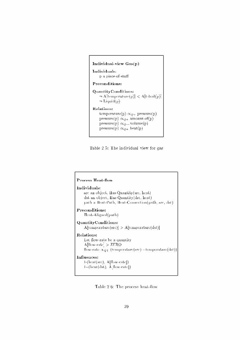
Processes are similar to views, except that they represent changes in the properties of

the individuals. These changes are represented by in uences. They describe the changes

that occur when the process is active. In table 2.6 the heat- ow process is given as an

example. This process describes how an energy ow can exist between two objects, a source

and a destination, when the temperature of the source is higher than the temperature of

the destination. The changes that this process introduces are: a decrease in the total

10Preconditions should represent external conditions, that is, aspects of the domain that are not ac-

cessible for the qualitative reasoner. For example, a heat-path in a heat- ow process should be a heat-

aligned(path) in order for the process to be applicable, but there is no way in which the qualitative reasoner

itself can in uence, or change, the status of this path.

19

Individual-view Gas(p)

Individuals:

p a piece-of-stu�

Preconditions:

QuantityConditions:

: A[temperature(p)] < A[t-boil(p)]

: Liquid(p)

Relations:

temperature(p) /Q+ pressure(p)

pressure(p) /Q+ amount-of(p)

pressure(p) /Q� volume(p)

pressure(p) /Q+ heat(p)

Table 2.5: The individual view for gas

Process Heat- ow

Individuals:

src an object, Has-Quantity(src, heat)

dst an object, Has-Quantity(dst, heat)

path a Heat-Path, Heat-Connection(path, src, dst)

Preconditions:

Heat-Aligned(path)

QuantityConditions:

A[temperature(src)] > A[temperature(dst)]

Relations:

Let ow-rate be a quantity

A[ ow-rate] > ZERO

ow-rate /Q+ (temperature(src) - temperature(dst))

In uences:

I-(heat(src), A[ ow-rate])

I+(heat(dst), A[ ow-rate])

Table 2.6: The process heat- ow

20

amount of energy in the source and an increase in the total amount of energy in the

destination.

2.2.2.3 Dependencies between Quantities

Four types of dependencies between quantities are used in the process centred approach

for modelling the properties of a con�guration of objects.

Inequalities These relations are used to represent inequalities between quantities. The

following relations are used:

� X < Y (X is less than Y )

� X � Y (X is less than or equal to Y )

� X = Y (X is equal to Y )

� X � Y (X is greater than or equal to Y )

� X > Y (X is greater than Y )

Inequalities are typically used to represent conditions that must be true in order for

an individual view to be applicable.

Proportionalities These relations represent functional dependencies between quanti-

ties. They are used to model how a certain quantity will change in its dependency

on another quantity. The following two relations are used:11

� X /Q�Y (X is decreasing monotonic in its dependence on Y )

� X /Q+ Y (X is increasing monotonic in its dependence on Y )

The idea here is that there exists some monotonic function that can be used to

determine the change of one quantity on the basis of how another quantity changes.

Consider, for example, the following dependency speci�ed in the individual view

gas. The proportionality relation pressure(p) /Q+ amount-of(p) de�nes that the

change in the pressure is increasing monotonic in its dependence on the amount-of.

In other words, changes in the pressure are determined by changes in the amount-

of. Increasing monotonic means that the changes of the two quantities are in the

same direction. The proportionality relation pressure(p) /Q�volume(p) (also from

the individual view gas) is similar to the previous one, expect that it speci�es a

monotonic decreasing dependency. This means that the changes of the two quantities

are in the opposite direction (see also table 2.7).

Correspondences These relations are used to relate speci�c qualitative values. Forbus

gives the example of the relation between the force exerted on an elastic band and

the length of this band. Qualitatively speaking we have no information about what

length of the band corresponds to what force, except for one. Namely, when the

band is at its rest-length we know that the exerted force is zero. Correspondences

can be used to model these speci�c relations between quantities.

11Forbus also de�nes the unknown dependency between two quantities: X /Q Y . This dependency

de�nes that X wants to change if Y changes, but it does not specify how.

21

X /Q+ Y X /Q�Y

�Y = + �X = + �X = �

�Y = 0 �X = 0 �X = 0

�Y = � �X = � �X = +

Table 2.7: Interpreting the e�ect of a single proportionality

In uences These relations may only appear in process de�nitions and are used for

representing changes. The following relations are used:12

� I-(X; Y ) (a negative in uence: X is decreasing monotonic in its dependence on

the qualitative value of Y )

� I+(X; Y ) (a positive in uence: X is increasing monotonic in its dependence on

the qualitative value of Y )

In contrast with proportionalities, in uences do not relate changes of quantities, but

relate the change of the dependent quantity to the value of another quantity. In the

de�nitions given above the qualitative value of Y determines the change of X . In

the case of I-(X; Y ), for example, this means that: if the value of Y is greater than

zero, X decreases; if the value of Y is equal to zero, it has no e�ect on X ; and so on

(see also table 2.8).

I+(X; Y ) I-(X; Y )

Y = + �X = + �X = �

Y = 0 �X = 0 �X = 0

Y = � �X = � �X = +

Table 2.8: Interpreting the e�ect of a single in uence

In most cases, if not all, in uences refer to some kind of ow rate that represents an

exchange between two objects. The speed of the exchange is captured by the value

of ow rate, whereas the e�ects of the exchange are represented by how the ow rate

changes the derivatives of certain quantities.

2.2.2.4 Reasoning with Multiple Dependencies

A change enforced upon a quantity by an in uence or a proportionality does not automat-

ically imply that the dependent quantity actually changes as speci�ed by that dependency.

If more than one dependency exists, it may happen that the resulting change in a quantity

is ambiguous and therefore in a certain state di�erent from what one of the dependen-

cies tried to enforce on it. In table 2.9 the calculus is presented for reasoning with two

proportionalities e�ecting a single quantity. Let us take, for example, the case in which:

(X /Q+ Y ) & (X /Q�Z) and (�Y = �) & (�Z = �). The proportionalities respectively

de�ne a monotonic increasing and decreasing relation for X in its dependence on Y and

12Forbus also de�nes the unknown in uence: I � (X;Y ). It de�nes Y in uences X, but it does not

specify how.

22

X /Q+ Y X /Q+ Y X /Q�Y

X /Q+ Z X /Q�Z X /Q�

Z

�Y = +

�Z = + �X = + �X =? �X = �

�Y = +

�Z = 0 �X = + �X = + �X = �

�Y = +

�Z = � �X =? �X = + �X =?

�Y = 0

�Z = � �X = � �X = + �X = +

�Y = �

�Z = � �X = � �X =? �X = +

�Y = �

�Z = + �X =? �X = � �X =?

Table 2.9: Determining change with multiple proportionalities

Z. Furthermore both Y and Z decrease. This means that Y tries to decrease X whereas

Z tries to increase it. The resulting change in X cannot be determined unambiguously

and will lead to three possible behaviours: one in which X increases, one in which X stays

constant, and one in which X decreases. However, if Y was increasing (as in the case of:

(�Y = +) & (�Z = �)), then the resulting change in X would not have been ambiguous,

X would start to increase as well.

For the in uences a calculus similar to the proportionalities can be applied, except

that for in uences the values of the in uencing quantity determine how the dependent

quantity changes. The calculus is given in table 2.10.

I+(X; Y ) I+(X; Y ) I-(X; Y )

I+(X;Z) I-(X;Z) I-(X;Z)

Y = +

Z = + �X = + �X =? �X = �

Y = +

Z = 0 �X = + �X = + �X = �

Y = +

Z = � �X =? �X = + �X =?

Y = 0

Z = � �X = � �X = + �X = +

Y = �

Z = � �X = � �X =? �X = +

Y = �

Z = + �X =? �X = � �X =?

Table 2.10: Determining change with multiple in uences

In the case of ambiguity, it does not really matter how many in uences or proportion-

alities have an e�ect on a certain quantity. The resulting change in the dependent quantity

23

will simply stay ambiguous, regardless of how many in uences or proportionalities are ac-

tive. In later publications this approach has been somewhat re�ned, in particular, taking

into account the strength of each individual in uence and proportionality [73] may lead

to resolving ambiguity in some cases.

2.2.2.5 Direct and Indirect Causality

Forbus distinguishes between changes that are caused directly or indirectly. Direct changes

are modelled by in uences (in processes), whereas indirect changes are modelled by pro-

portionalities. Forbus refers to this as the causal directness hypothesis: changes in physical

situations which are perceived as causal are due to our interpretation of them as corre-

sponding either to direct changes caused by processes, or propagation of those direct e�ects

through functional dependencies. This hypothesis puts three further constraints on how

the in uences and proportionalities should be applied. Firstly, all changes are initialised

by in uences. Without an in uence, or for that matter a process, there is no change

and therefore no behaviour in the physical world. The proportionalities are used to prop-

agate changes, introduced by in uences, throughout the whole system. Secondly, both

in uences and proportionalities are directed, i.e. their e�ect propagates in one direction

only. The in uencing quantity (right hand side, of both in uences and proportionalities)

has to be known before the dependent quantity can be determined (left hand side). The

relations may not be used the other way around, because this would violate the causal

chain of changes, which is one of the essential features of the process centred approach.

Thirdly, no quantity may be in uenced directly and indirectly simultaneously. According

to Forbus, a physics that allows a quantity to be in uenced both directly and indirectly

at the same time must be considered inconsistent, because it also violates the essential,

non-recursive, chain of causality.13

2.2.2.6 Supertype and Applies-to Relations

Processes and individual views may require other processes or individual views to exist

before they are applicable. This is shown in the boiling process in table 2.11: before boiling

can be applied the process heat- ow must exist.

In addition to being conditional, processes may have subtype (is-a) relations. The

more speci�c process inherits all the relations and in uences of the more general type. In

table 2.12 an example is given in which the processes slide and roll are de�ned as subtypes

of motion.

2.2.2.7 Scenarios and Domain Models

In later publications [67; 68], sets of views and processes are distinguished, and referred

to as di�erent domain models. The idea here is that each physics domain has its own

speci�c set of individual views and processes that describes its features. This grouping of

individual views and processes into subsets is one of the techniques that is being developed

to cope with the problem of reasoning with large scale qualitative models. Some of the

examples given are:

13Notice, that this requirement excludes representing feedback loops.

24

Process Boiling

Individuals:

w a contained-liquid

hf a process-instance, process(hf) = heat- ow

^ dst(hf) = w

Preconditions:

QuantityConditions:

Status(hf, Active)

: A[temperature(w)] < A[t-boil(w)]

Relations:

There is g 2 piece-of-stu�

gas(g)

substance(g) = substance(w)

temperature(w) = temperature(g)

Let generation-rate be a quantity

A[generation-rate] > ZERO

generation-rate /Q+ ow-rate(hf)

In uences:

I-(heat(w), A[ ow-rate(hf)])

I-(amount-of(w), A[generation-rate])

I+(amount-of(g), A[generation-rate])

I-(heat(w), A[generation-rate])

I+(heat(g), A[generation-rate])

Table 2.11: The process boiling

� The contained stu� ontology, used for uids and their tanks. Similar to classical

thermodynamics.

� The energy ow ontology, analyses energy ow and is concerned with both heat and

work.

� The molecular collection ontology, describes the movement of uid molecules during

ow.

� The mechanics ontology, used for analysing the dynamics of mechanisms.

Once all the library knowledge has been modelled the next step is to provide the

qualitative reasoner (QPE)14 with a description of the system that is the object of the

reasoning process. In the process centred approach such a description is called a scenario.

14Forbus refers to his latest implementation of his process centred approach (the Qualitative Process

Theory (QPT)) as the Qualitative Process Engine (QPE) [73]. His �rst implementation of QPT is calledGIZMO [71].

25

Process Motion(B,dir)

Individuals:

B an Object, Mobile(B)

dir a direction

Preconditions:

Free-direction(B,dir)

Direction-Of(dir,velocity(B))

QuantityConditions:

Am[Velocity(B)] > ZERO

In uences:

I+(positive(B),A[velocity(B)])

Process Slide

Case-of: Motion

Individuals:

S a surface

Preconditions:

Sliding-Contact(B,S)

AlongSurface(dir,B,S)

Process Roll

Case-of: Motion

Individuals:

S a surface

Preconditions:

Contact(B,S)

Round(B)

AlongSurface(dir,B,S)

Table 2.12: The processes slide and roll are subtypes of the process motion

An example of such a scenario is given in table 2.13 (for the U-tube as depicted in �gure

2.10).

2.2.2.8 Finding Applicable Individual Views and Processes

Given a scenario, the qualitative reasoner needs to search for individual views and processes

that apply to it. For each collection of objects that satis�es the description of the required

individuals for a view or a process, a view-instance or a process-instance is created. If

the preconditions and quantity conditions for such a view-instance or process-instance are

true, the instance is given the status of being active. It receives status inactive otherwise.

There is a dependency problem here, in the sense that for some instances to be active

others must �rst be active. For example, the process boiling can become active only after

the process heat- ow has become active. The algorithm needed for implementing this

problem solving behaviour may turn out to be ine�cient, in its worse case it has to check

26

;structural description

Open-Container(C)

Open-Container(D)

Fluid-Path(P)

Fluid-Connected(C,D,P)

;some substances are in the containers

Contains-Substances(C,Water)

Contains-Substances(D,Water)

;the levels are related

Level-in(C,water) > Level-in(D,water)

Table 2.13: Scenario for the U-tube

every inactive instance for its status after a new instance has become active. Special care

has to be taken in order to keep the performance level of the prediction engine acceptable.

In the QPE implementation an ATMS technique [54; 55; 56] is used for this purpose.15

There is a second problem with determining the applicability of individual views and

processes, namely reasoning with inequalities. Inequalities are used extensively in the pro-

cess centred approach and therefore sophisticated techniques are required. In particular,

those concerning transitivity, as shown in table 2.14 (cf. [120]).

A > B ^B > C ) A > C

A = B ^B = C ) A = C

A > B ^B = C ) A > C

Table 2.14: Examples of transitivities

2.2.2.9 Limit Analysis

Given the set of applicable views and processes, the direct in uences of the processes are

determined �rst. Next, the e�ects of these in uences are propagated by the available

proportionalities, resulting in a complete description of all the changes in the current

situation, i.e. the derivatives of all quantities are determined. This behaviour description

15In [73] Forbus refers to domain models in which processes (or individual views) require other processes

(or individual views) to be active �rst as ill-conditioned QP models and claims that it is always possibleto create a well-conditionedQP model out of an ill-conditioned one (by adding the necessary conditions).

We disagree with this point of view, because although the claim is in principle correct, it undermines the

idea that incremental models can be created by using part-of and is-a dependencies between processes andindividuals views. This issue is further discussed in section 4.2.1.6.

27

is then analysed in order to �nd out whether the changing behaviour of the system becomes

incompatible with this description. This is called limit analysis. It uses the derivatives

and the quantity spaces, to determine how the inequality dependencies between quantities

may change. Take, for example, the quantity space in �gure 2.10. If we assume that

level(WD) increases, �level(WD) = +, then after some time has elapsed this quantity

will become equal to either height(top(D)) or to level(WC) (or to both). These values are

the so called limit points that the increasing water level may reach as time passes. Each

changing quantity and all possible consistent combinations of these changing quantities,

form the quantity hypotheses. All the sets present in this quantity hypotheses that have

at least one quantity that will actually reach a limit point, and thereby cause a change in

the current set of active individual views and processes (as opposed to just indicating a

change), form together the set of limit hypotheses for the current state of behaviour.

2.2.2.10 Ambiguity

The quantity hypotheses often represents a number of possible state terminations because

of ambiguity. Three sources of ambiguity are:

� The quantity space is only partially ordered and therefore it is undecidable which

limit point a quantity will reach. Each possible limit point represents a possible

state termination.

� One process may in uence more than one quantity. If these quantities are indepen-

dent, they may lead to multiple state transitions.

� More than one process may be active and these may have opposing e�ects on the

derivative of a speci�c quantity. The behaviour of the quantity is then ambiguous

and multiple state terminations may occur.

2.2.2.11 Determining State Transitions

Forbus points out three types of knowledge which can be used for deciding among possible

state transitions:

� Certain changes may invalidate other changes. For example if an individual vanishes,

then all other changes (parameters) regarding this individual become irrelevant.

� State transitions must be continuous, that is, quantities must change via adjacent

points in the quantity space. Discontinuous changes can therefore be discharged.

� Domain speci�c knowledge. For example, the pressure increase resulting from heat-

ing liquid is negligible with respect to the pressure increase from heating a gas.

Therefore, the result from an increasing liquid pressure will be overruled by an in-

creasing gas pressure.

The limit analysis speci�es what will change from the current state of behaviour to the

next state of behaviour. For each hypothesis present in the limit hypotheses, which has

not been invalidated because of reasons described above, the qualitative reasoner will have

to determine the corresponding next state. Essentially this activity involves two aspects:

28

�rst �nding out which individual views and processes from the old state of behaviour

are no longer applicable anymore, and second, determining which new individual views

and processes might be applicable in the next state of behaviour. With respect to the

latter there are again two possibilities, either the state has been generated before, or it

is a new state. In the case of an already known state of behaviour the reasoning about

that particular state stops, because it has previously been analysed. For each new state,

the reasoning process has to be repeated. The qualitative reasoning process as a whole

continues until for each state of behaviour a complete interpretation has been generated

and all the possible transitions between these states have been determined.

2.2.2.12 Attainable and Total Envisionments

In [73] the above described limit analysis is implemented di�erently. Forbus discriminates

therefore between a total envisionment and an attainable envisionment. A total envision-

ment is de�ned as having no speci�c initial state, but every state consistent with a given

scenario must be generated. An attainable envisionment consists of all states that can be

reached by some set of transitions from a distinguished initial state. A total envisionment

is in fact the union of attainable envisionments from every possible initial state. The limit

analysis described above realises an attainable envisionment (GIZMO), whereas QPE

realises a total envisionment. The distinction can easily be understood if we consider the

U-tube example as depicted in 2.10. An attainable envisionment would not generate the

state of behaviour in which both tanks are empty, because that state cannot be reached

from the initial state. A total envisionment would derive this state of behaviour. The

crucial distinction between the two envisionments relies on how the inequality relations

are used by the qualitative reasoner. In the case of a total envisionment they are used

as the overall set of conditions that specify the requirements for a certain state of be-

haviour. In case of an attainable envisionment the inequality relations are used in a more

restricted way, the inequality relation speci�ed in the scenario has to be true for each state

of behaviour that is generated on the basis of the scenario. Obviously, adding inequality

relations to a scenario used by a total envisionment is of no use.16

2.2.3 Constraint Centred Approach

Kuipers describes the constraint centred approach [92; 93]. His approach takes a quali-

tative version of a di�erential equation, used in traditional physics for generating numer-

ical or analytic solutions, as a starting-point (see �gure 2.11). The basic assumption is

that ordinary di�erential equations (ODE's) can be rewritten into qualitative di�eren-

tial equations (QDE's). The qualitative di�erential equations can be used for qualitative

simulation. The simulation process should provide a description of the actual real-world

behaviour.

2.2.3.1 Mapping ODE's onto QDE's

In the constraint centred approach there is no explicit representation of entities from the

real-world. This approach also does not use a library of any kind from which models can be

16Notice that a total envisionment is always relative to the knowledge speci�ed in the individual views

and processes.

29

Physicalsystem

Differentialequation

Qualitativeconstraints

numerical or analytic solution

qualitative simulation

Actualbehavior

Behavioraldescription

i→RR RRƒ :

Figure 2.11: Qualitative simulation, di�erential equations and actual behaviour

selected during simulation. Instead, the qualitative reasoner (QSIM)17 is provided with

a description of some aspect of the (physical) world in terms of the qualitative constraints

shown in table 2.15. Each of the constraints maps onto a speci�c aspect of the ordinary

di�erential equations.

Qualitative constraints (QDE's) Ordinary equations (ODE's)

ADD(f; g; h) f(t) + g(t) = h(t)

MULT(f; g; h) f(t):g(t) = h(t)

MINUS(f; g) f(t) = �g(t)

DERIV(f; g) f 0(t) = g(t)

M+(f; g) f(t) = H(g(t)) ^ H 0(x) > 0

M�(f; g) f(t) = H(g(t)) ^ H 0(x) < 0

Table 2.15: Qualitative constraints and ordinary equations

2.2.3.2 Setting up a Constraint Model

According to Kuipers each system is characterised by a number of real-valued parameters,

which continuously vary over time. So called reasonable functions (in table 2.15: f , g and

h) are used for modelling the time-varying aspect of these parameters. In �gure 2.12 such

a constraint model is given for the U-tube.

The constraints

M+(Level(A); Pressure(A))

and

M+(Level(B); Pressure(B))

represent the fact that changes in the level of a tank correspond to similar changes in the

pressure at the bottom of that tank. The constraint

ADD(Pressure(B); PressureDifference; Pressure(A))

17The qualitative reasoning program that implements the constraint centred approach has been given

the name QSIM [93].

30

M +ddt

ddt

M +

Level(A)

Pressure(A)

M +

Level(B)

Pressure(B)

Pressure Difference

Flow Rate (A B)→

A B

Figure 2.12: A constraint model of the U-tube

shows how the pressure di�erence between tank A and tank B is calculated. This pressure

di�erence changes proportionally to the ow rate between tank A and tank B, which is

represented in

M+(PressureDifference; F lowRate(A! B))

Finally, the

DERIV (Level(B); F lowRate(A! B))

and the

inverseDERIV (Level(A); F lowRate(A! B))

represent how the ow rate e�ects the levels in each tank, namely when the ow rate goes

from A to B (FlowRate > 0) then the level of tank A will decrease and the level of tank

B will increase.

Qualitative constraint models, such as the one described above, can in principle be gen-

erated by rewriting the di�erential equations that are used in traditional physics. However,

this is not a necessity, in the sense that there is no restriction on how these models are

created. It is possible to formulate constraint models for domains that have not been

tackled by traditional physics. Typical examples in this respect are the constraint models

that have been developed in medical domains (cf. [94; 96; 86; 43; 130]).

2.2.3.3 Landmarks and Initial Values

For behaviour prediction with the constraint centred approach two additional aspects must

be de�ned: the initial values of parameters and the landmarks. The landmarks represent

a �nite set of values for each function that is used for modelling the system. Landmarks

are critical in the sense that they correspond to essential changes in the behaviour of the

system. The landmark values for level(A) could, for example, be f0; p; infinityg, referring

to landmarks at value 0, at some point p (between 0 and infinity), and at infinity. Given

this set of landmarks the parameter level(A) can take one of these values, or a value in

between two landmarks. As an initial value for level(A) we could specify that the value

is somewhere between p and infinity and that the value is increasing. The idea behind

31

this initial value is that, as shown in �gure 2.12, some amount of liquid is added to tank

A, which disturbs the equilibrium and therefore leads to behaviour in the U-tube system.

2.2.3.4 Upper and Lower Boundaries

Functions in constraint models may have upper and lower range limits, which are landmark

values beyond which the current set of constraints no longer applies. A range limit may

be associated with a new operating region which has its own constraints and range limits.

By using this mechanism multiple constraint models can be de�ned for a single system,

each model referring to a di�erent type of behaviour manifested by the system.

2.2.3.5 Generate and Test

Behaviour prediction with constraint models is done by applying a generate and test18 cycle

that produces the possible behaviours of a system. Testing is concerned with determining

the consistency of a certain state, by applying constraint satisfaction to the constraint

model that represents the behaviour in that state. The generation part determines how a

state of behaviour may change into a new state of behaviour, by applying transition rules

to each function in the current state of behaviour (see table 2.16). All distinct sets of

transition rules, specifying a particular transition for each function in the current state,

may lead to new states of behaviour.

2.2.3.6 Interval and Point Transitions

Kuipers introduces the notion of time-points. A state of behaviour refers to functions either

being at a time-point or being in between two time-points. In each state of behaviour a

function is:

� either at a landmark or in between two landmarks, and

� increasing, decreasing or steady.

However, function values can only change:

� from having a landmark value, (lj), to having a value in between two landmarks,

(lj; lj+1) or (lj�1; lj), while going from a time-point, (ti), to a time interval in between

two time-points, (ti; ti+1), and

� from having a value in between two landmarks, (lj ; lj+1), to having a landmark, (lj)

or (lj+1), while going from a time interval in between two time-points, (ti; ti+1), to

a time-point, (ti+1).

In table 2.16 these value changes are referred to as the P-transitions and the I-transitions.

The P-transitions P1, P5 & P7 and the I-transitions I1, I4 & I7 di�er from the other

transitions, because they allow functions to keep the same value while changing time-

points (a function stays constant at a landmark, a function keeps increasing between

18Notice that this generate and test cycle is not the same as the generate and test cycle used by de Kleer

(see section 2.2.1.6).

32

P-transitions I-transitions

QS(f; ti) )QS(f; ti; ti+1) QS(f; ti; ti+1) )QS(f; ti+1)

P1 hlj , stdi )hlj , stdi I1 hlj, stdi )hlj , stdi

P2 hlj , stdi )h(lj ; lj+1), inci I2 h(lj; lj+1), inci )hlj+1, stdi

P3 hlj , stdi )h(lj�1; lj), deci I3 h(lj; lj+1), inci )hlj+1, inci

P4 hlj , inci )h(lj ; lj+1), inci I4 h(lj; lj+1), inci )h(lj; lj+1), inci

P5 h(lj; lj+1), inci )h(lj ; lj+1), inci I5 h(lj; lj+1), deci )hlj , stdi

P6 hlj , deci )h(lj�1; lj), deci I6 h(lj; lj+1), deci )hlj , deci

P7 h(lj; lj+1), deci )h(lj ; lj+1), deci I7 h(lj; lj+1), deci )h(lj; lj+1), deci

I8 h(lj; lj+1), inci )hl�, stdi

I9 h(lj; lj+1), deci )hl�, stdi

Table 2.16: Transition table for P- and I-transitions

two landmarks and a function keeps decreasing between two landmarks.) There is no

conceptual di�erence between P1 & I1, P5 & I4, and P7 & I7, except for their speci�c

relation with time-points.

Also di�erent are the I-transitions I8 and I9. These transitions create new landmarks.

The idea here is that it is in principle always possible to `discover' a new landmark in

between two known landmarks. In other words, it is possible for the system, or parts of

it, to reach an equilibrium at points that were not anticipated during the construction

of the constraint model. For example, in the U-tube, the system reaches an equilibrium

with both level(A) and level(B) being higher than they were before liquid was added to

tank A. The constraint centred approach explicitly derives that the system reaches an

equilibrium with higher levels in each tank. The method used to detect new landmarks

is straightforward: when a function is increasing or decreasing between two landmarks,

assume that the function will reach a new landmark (at the next time-point) somewhere

in between the two landmarks within which the function is changing. The only additional

requirement put on `discovering' new landmarks is that the function becomes steady when

it reaches this new landmark.

It is probably the `simplicity' of the method that also leads to its greatest drawback,

namely that very often endless numbers of new landmarks are created.19 Take, for exam-

ple, the behaviour of a bouncing ball. Each time the ball goes into the air after bouncing,

its speed decreases because of gravitation. At some point in the air this speed becomes

zero. After the ball has reached this highest point it falls back to earth and bounces again.

This time, however, its highest point will be lower than the previous one, because of fric-

tion and loss of energy. Eventually, the total loss of energy will be such that the ball stops

bouncing. One of the problems with the constraint centred approach for modelling the

bouncing ball is that although it derives that the height will be less after each bounce of

the ball, it does not derive that this necessarily leads to the ball remaining on the ground.

Instead it keeps introducing new landmarks in between the ground and the latest highest

point it reached.

19QSIM simulations often never stop as a result of continuously creating new landmarks. The programtherefore has an option to restrict the maximum number of states that it may predict.

33

2.2.3.7 Testing State Transitions

The testing part of the cycle determines whether a new state of behaviour is actually going

to exist on the basis of (1) its internal consistency and (2) whether the global �lters allow

it to become active. Internal consistency is checked by the constraint satisfaction method.

It is done by creating all possible tuples (pairs or triples) for the transitions found for the

functions present in each single constraint. Given these tuples the consistency checking

proceeds by applying the following three steps:

Constraint consistency Transitions applied to the functions present in a single con-

straint must be consistent with that constraint. For example, if two functions have

an M+ constraint then they should have the same direction of change in the next

state of behaviour.

Pairwise consistency �ltering After constraint consistency it should still be possible

for two constraints that restrict the same function (so called adjacent constraints)

to �nd tuples that provide the same transition for that function. Each tuple that is

not pairwise consistent will never lead to a consistent new state and therefore has

to be removed. Suppose, for example, that the constraint M+(f; g) has transition

tuple (I2, I2). Pairwise consistency speci�es that if there are other constraints on

the functions f and g then the transition tuples associated with those constraints

should at least allow the I2 transition for both f and g.

Generating global interpretations A global interpretation is an assignment of a

transition to each function in the system. Not all combinations of remaining tuples

(after constraint and pairwise consistency �ltering) are possible global interpreta-

tions. First of all, because of a reduced set of transitions, it may be the case that a

transition cannot be found for each function. There is no transformation to a new

state of behaviour if this happens. Second, even if a transition can be found for

each function, this does not necessarily imply that the total set of transitions (the

global interpretation) is consistent. A certain amount of pruning has to be done to

guarantee a consistent transformation to a new state of behaviour. If, for example,

M+(f; g) has transitions tuples (I2, I2) and (I3, I3) and M+(g; h) has transitions

tuples (I2, I2) and (I3, I3), then the combination of I2, I2, and I2 for f , g and h

represents a consistent global interpretation, but the combination of I2, I2, and I3

for f , g and h does not.

If a new state of behaviour is internally consistent, this does not necessarily imply

that this state of behaviour will exist. There are essentially three global �lters that may

prevent such a state of behaviour from becoming active:20

No change At least one function must reach a landmark or move from a landmark

in order to ensure that the new state of behaviour is di�erent from its immediate

predecessor. In other words, if all the transitions in a global interpretation are either

in the set fI1, I4, I7g or in the set fP1, P5, P7g then nothing has changed and the

new state of behaviour will not become active.

20In later publications additional �lters have been proposed (cf. [95]).

34

Cycle If a new state of behaviour is identical to one of its predecessors (all functions

have the same landmark values and the same direction of change), then the new

state of behaviour does not become active. The behaviour is marked as cyclic and

instead of pointing to the new state of behaviour the transformation will be to the

old state of behaviour.

Divergence If any function takes on the value 1 or �1, then (by de�nition) the

current time point must be the end of the domain, so the new state of behaviour

will not become active.

The total cycle of generating new states of behaviour and determining their internal

consistency stops when no more transitions can be found that transform an old state of

behaviour into a consistent and permitted new one.

2.3 Problems with the Current Approaches

This section discusses outstanding problems that occur when using the original approaches

to qualitative reasoning. Each subsection starts with a brief summary of the approach,

followed by a number of subsections that describe the problems.

2.3.1 Component Centred Approach

The component centred approach models the physical world as consisting of components

that manipulate materials and share information by means of conduits. Components

behave independently from their surroundings, they obey the no-function-in-structure

principle. How components manipulate materials is described in the library of component

models. In these descriptions the behaviour of a component is represented as con uences,

which are relations between parameters that describe the characteristics of the materials.

One component can have a number of qualitative states in its component model, each

specifying a particular state of behaviour and associating it with a particular group of

con uences.

For performing qualitative reasoning the program must be given an (initial) system

description, called the system topology. Based on this con�guration of components and

conduits the program generates a cross-product of qualitative states, i.e. each qualitative

state of one component is combined with each qualitative state of the other components.

Every combination refers to a possible state of behaviour in which the system can be.

Given these overall states of behaviour, the internal consistency of each state of be-

haviour is determined by applying constraint satisfaction and generate and test. The con-

sistent states of behaviour are then analysed for state transitions by determining whether

certain transformation rules are true between two states of behaviour. The �nal result of

all these activities is a total envisionment, i.e. a set of state descriptions with for each

description speci�ed: its internal behaviour in terms of parameter values, its preceding

states and its successor states. Together they describe all possible behaviours of the system

speci�ed in the initial description.

35

2.3.1.1 Using Component Models

There is some ambiguity as to how the component models relate to a system in the

physical world. They might be straightforward abstractions of physical components that

actually exist in the physical world, or they might be abstractions of processes and not

necessarily correspond to components that exist in the physical world. Both views appear

to be problematic. In the latter case the approach does not support deriving behaviour

from structure, because the structure itself cannot be taken as the basis for identifying

components. Consider, for example, the two wires in �gure 2.13. Because there is a current

F2F1F2F1

wire1 wire2 wire1 wire2

Figure 2.13: Wires moving towards each other

ow through each wire it senses the magnetic �eld of the other. The resulting forces are

such that the wires are attracted to each other since the currents are in the same direction.

In this example it is not possible to derive the behaviour of the system without taking

the interaction between the components into account, but there is no physical component

that represents this interaction. In other words, there is no direct relation between the

physical structure and the system topology, and the corresponding component models,

needed for reasoning about this system. A modelling step is required which translates the

physical structure in real-word to an adequate con�guration of canonical components and

conduits.

In situations where the components and conduits represented in the system topology

directly relate to the objects existing in the physical world, there is still the problem that

the behaviour of the components sometimes depends on the speci�c context in which they

operate. In other words, the no-function-in-structure principle cannot always be obeyed.

Take, for example, the behaviour of the U-tube (see �gure 2.5). Instead of using three

components we could have modelled this system as consisting of two components (con-

tainers) connected by a conduit. Each container has four qualitative states of behaviour:

steady, which means that the total amount of liquid remains constant, decreasing or in-

creasing, which means that liquid is owing out or owing in and empty, which means

that there is no liquid present in the container (see �gure 2.6). It is easy to see how the

cross-product of the 4 qualitative states for both components result in 16 (4x4) overall

state descriptions and how the �nal behaviour can be derived from this as a sequence of

valid state descriptions.

This model predicts the behaviour of the connected containers correctly and also relates

directly to the objects existing in the physical world, but it does not explain why the

components behave as they do. It cannot be derived that there is a pressure di�erence

between the liquids in the two containers and that therefore a liquid ow arises.

In order to model this causal notion a third component can be introduced (see �gure

2.5) with slightly `arti�cial' states of behaviour. Namely, modelling the pipe as a valve-

36

like connector with four qualitative states of behaviour, based on the pressure di�erence

between input and output (see �gure 2.6). Again it is easy to see how the cross-product

of these qualitative states results in 64 (4x4x4) overall state descriptions (most of them

inconsistent of course) and how the �nal behaviour can be derived from this as a sequence

of valid state descriptions.

However, two problems still exist. Firstly, the introduction of an arti�cial component

brings us back to the problem discussed above, i.e. not having a direct relation between

the structure and the components used in the qualitative reasoning process. Secondly,

even though the pressure di�erence is represented as a speci�cation for the liquid ow in

the valve, it can still not be derived that the di�erence in height for the two liquid columns

causes the pressure di�erence.21

In summary, the interactions between components, that in some situations cause be-

haviour, cannot be modelled adequately when the no-function-in-structure principle is

applied. Therefore, in order to build realistic models of the physical world that capture

the essential aspects of its behaviour, we must incorporate the fact that in some cases

there is function-in-structure.

2.3.1.2 The Cross-product

Given a con�guration of components and conduits, the overall behaviour is generated by

�rst taking the cross-product of the qualitative states of the components. The mathe-

matical models that are generated in this way are then given to the constraint satis�er to

test their validity. Finally, the consistent models (valid states of behaviour) are ordered

according to a set of rules. The state diagram resulting from this represents the overall

behaviour of the device.

The cross-product technique has two drawbacks, it is counter-intuitive and it is li-

able to combinatorial explosion. These drawbacks are particularly problematic if someone

wants to use the prediction machinery interactively for building qualitative models. Imag-

ine debugging a simple model of 10 components, each with 5 qualitative states. The

cross-product generates 9,765,625 possible states and the constraint satis�er will probably

discharge most of them as being inconsistent. Even if the machinery is strong enough to

handle all these states, then it still is completely impossible to trace back errors in this

model. The technique does not provide the user with any clues as to what qualitative

state, con uence, or speci�cation might be erroneous.

A directed, depth-�rst or best-�rst search, that gradually builds up the model by

selecting and evaluating one qualitative state at the time seems to be essential. This

technique is more intuitive, provides feedback as to what qualitative state, speci�cation

or con uence, was not applicable at a certain point in the inference process, and it puts

less burden on the capacity of the machinery.

2.3.1.3 Causal Explanations are Troublesome

Con uences specify dependencies between parameters, but cannot represent causal rela-

tions between parameters. Direct causal explanations are therefore not possible. Some

techniques have been proposed to enhance constraint satisfaction so that a causal avour

21This is essentially why in �gure 2.7 and in �gure 2.8 the containers have all equal heights.

37

appears. Mythical causality [57] and causal ordering [87] are two of those. Both techniques

are based on the same underlying principle: try to detect exogenous parameters from

which a causal structure or propagation trace can be derived. Although these techniques

are useful they seem to ignore the fact that in some situations the available knowledge

is more speci�c than can be modelled by con uences. Take, for example, the model of a

refrigerator as described by Iwasaki and Simon. One of the equations speci�es the relation

between the condensing temperature of the refrigerant and its pressure:

Tc = f(P )

This relation only speci�es that there is a dependency and does not capture the general

knowledge that changes in the pressure of a substance cause the condensing temperature

of the substance to change (and not the other way around!).

It appears that by only using con uences a certain amount of general knowledge about

causality is lost, which unnecessarily complicates the process of providing causal expla-

nations. It is important to also use relations between parameters with a more speci�c

semantics that represent the available causal knowledge directly.

2.3.2 Process Centred Approach

Important ontological primitives in the process centred approach are views and processes.

Views associate objects, or groups of objects, with parameter relations. These relations

describe how the characteristics of materials and of objects are related to each other. Pro-

cesses are similar to views, except that they can in uence the characteristics of materials

and objects.

For performing qualitative reasoning the program must be given an initial system

description (scenario) consisting of a collection of physical objects and possibly some

inequality relations between the quantities that describe the properties of these objects.

The program then searches for views and processes that apply to that description. Given

the set of applicable views and processes, the in uences of the processes are determined

�rst. The e�ects of these in uences are then propagated by the available parameter

relations, resulting in a complete description of the current situation.

This description of the situation is then analysed in order to �nd out whether in

the future the behaviour of the system becomes incompatible with this description. The

process centred approach has a number of rules that specify how a particular situation

description terminates, as well as how a transition to another (new) situation description

can take place. With respect to this new situation description there are two possibilities,

either the description has been generated before, or the description is new. In the former

case the reasoning about that particular description stops, because it has previously been

analysed, but for each new description the reasoning process is repeated as described

above. The qualitative reasoning process as a whole continues until for each situation

description a complete interpretation has been generated and all the possible transitions

between these descriptions have been determined.

2.3.2.1 Semantics for Behaviour Models

To some extent within the process centred approach itself, but particularly when com-

pared with the component centred approach, there is a growing need for an integrated

38

semantics for behaviour models. How does for example the no-function-in-structure relate

to processes and views. Processes apparently do not obey this principle and are therefore

well suited for dealing with the interaction problem discussed in section 2.3.1.1. Both

the interaction between the two wires and the interaction in the U-tube can be modelled

by processes, because processes are triggered by inequalities that exist between similar

quantities of di�erent objects.

In [72] Forbus introduced actions into his process centred approach and refers to the

notion of background information, that normally does not change during the simulation

process, as the basis for introducing actions. However, he does not explain why processes

apparently only represent a speci�c category of changes. Why, for example, has motion,

that was described as a process in the earlier work [70; 75], now changed to being an

action?22

Finally, individual views described the static properties of physical objects. Some of

these individual views apply to a single `object', for example, an individual view for gas,

whereas others apply to a collection of physical objects, for example, an individual view

for a `contained liquid'. It is in this respect not clear how the individual views relate to the

no-function-in-structure principle. Do the individual views that apply to a single physical

object obey the no-function-in-structure principle?

In the component centred approach behaviour is modelled by a set of component mod-

els. These models represent both static properties and changes. Although some aspects

cannot be modelled adequately by components, they are well suited for representing the

behaviour of devices. It is not clear how component models relate to the notions of views

and processes.

Two typical questions that have to be answered by an integrated semantics for be-

haviour models are therefore:

� What type of changes are there, what type of modelling primitives are needed for

representing them and which guidelines can be used for distinguishing between them.

� What type of static properties are there, what type of modelling primitives are

needed for representing them and which guidelines can be used for distinguishing

between them.

The no-function-in-structure principle can probably be used as a guideline for answering

these questions.

2.3.2.2 Type of Knowledge versus Use of Knowledge

When studying the de�nition and some examples of views and processes it turns out that

there is a mixture between type of knowledge and use of knowledge, referring to what

knowledge is modelled and how that knowledge is used by the problem solver. Forbus

uses knowledge typing to de�ne views and processes, namely by discriminating between

individuals, preconditions, quantity conditions, relations, and in uences. However, some

of these types are implicitly seen as conditional whereas others represent additional in-

formation that holds if the view or the process holds. This implicit mixture is not only

22The process centred approach also anticipates that some changes in the physical world are too complex

to be modelled in detail and therefore allows the use of encapsulated histories. Such a history represents

the behaviour with less detail than a collection of views and processes.

39

confusing, but leads to de�nitions of views and processes that are `wrong'. For example,

`creating a gas' in the boiling process (see table 2.11) is speci�ed by the `relations'. Which

is strange because `gas' is not a `relation', but an `individual'. However, it cannot be part

of the `individuals', because `individuals' are used as conditional statements, which the

creation of `gas' is not. Another example is the `process heat ow' that should be active

for the `boiling process' to hold. `Individuals' and `quantity-conditions' are used to specify

the `process' and its 'status' respectively, but a `process' is not an `individual', in the sense

that it does not represent an `object from the physical world', and `being active' is not a

`quantity-condition', in the sense that it does not represent a number of `inequalities' that

should be true.

Mixing type of knowledge and how this knowledge is used by the problem solver should

be avoided, for enhancing the conceptual clarity of the modelling primitives and for unnec-

essarily confusing the modelling process. It is therefore relevant to discriminate between

conceptual (knowledge level) and computational (symbol level) knowledge (cf. [109]).

2.3.2.3 Causality is not Always Known

In section 2.3.1.3 we argued that the causality which is present in a domain should be

represented. The process centred approach is well equipped for this purpose by allowing

the representation of both direct and indirect relations. However, in some situations the

causal interpretation between related quantities is not so obvious. Consider, for example,

the relation between the input and the output currents of a closed switch:

Ioutput = Iinput

Using proportionality relations for modelling the dependency between the input and out-

put current is problematic for two reasons. Firstly, it is debatable whether there is a causal

relation between the input and the output current (does the input current cause the output

current?). Secondly, the dependency between the two parameters is more restricted than

can be represented by a proportionality relation. Both the values of the two parameters

and how they change, are always equal for the input and the output current when the

switch is closed. In particular, the equality between derivatives cannot be modelled by

the relations provided by the process centred approach.

2.3.3 Constraint Centred Approach

The constraint centred approach takes a qualitative version of the di�erential equation,

that is used in traditional physics for describing a particular situation, as a starting-point.

This (mathematical) model is input for a generate and test cycle that determines all the

possible behaviours of the modelled system. The total cycle stops when, similar to the

process centred approach, for each situation an interpretation has been generated and all

possible transitions between situations have been determined.

2.3.3.1 No Modelling Ontology

When compared with the component and process centred approach the constraint centred

approach di�ers on two important issues:

40

� it does not support deriving behaviour from the physical structure (instead QSIM

takes di�erential equations as a starting point), and

� the modelling primitives provided by this approach do not allow symbolic modelling

of the knowledge that people have of the every day physical world (notions such

as processes, static properties, and physical structure cannot be presented by this

approach explicitly).

Both these issues are essential aspects of qualitative reasoning. Experts, when faced

with analyzing properties of a new physical system, start by identifying relevant objects,

components and processes that appear in this system, and try to �nd out if the behavioural

model they built on top of this, matches the actual behaviour of the system. (This

qualitative model is then used to write down the di�erential equations that describe the

physical system in a formal way.) A similar kind of approach is used by non-experts

(except that they do not write down di�erential equations). An integrated approach to

qualitative reasoning should therefore be based on reasoning from structure.

2.3.3.2 No Knowledge about Inequalities

The constraint centred approach does not use inequality relations. Landmarks are only

ordered for a speci�c function. But the relation between landmarks for di�erent functions

is unknown, except for the fact that they may, or must be, reached by related functions

at the same time-point. There is no knowledge in a constraint model that represents that

a certain landmark is higher, lower or equal than some other landmark. In the case of the

U-tube (see �gure 2.12), for example, QSIM may generate a new landmark for each of the

liquid columns and derive that the U-tube reaches an equilibrium at these new landmarks.

However, it has no explicit knowledge about the inequality relation between the heights

of each column.

2.4 Concluding Remarks

In this chapter we have given descriptions of the current approaches to qualitative reason-

ing. In addition we have pointed out a number of problems that are still standing out for

each of the approaches.

Two important conclusions can be drawn from the overview presented in this chapter.

Firstly, none of the approaches completely captures all the distinctions that are relevant

for qualitative prediction of behaviour. Instead, each approach seems to be particularly

suited for modelling a certain part of this problem solving task. Secondly, although the

di�erent approaches show a certain amount of similarity, the precise relation between the

conceptualisations used in each of the approaches is unclear.

It seems therefore fair to conclude that there is a need for an integrated approach

to qualitative prediction of behaviour. Not only for pointing out the similarities and

di�erences between the individual approaches, but also for establishing a problem solving

potential that currently cannot be realised by either of the original approaches. The most

important requirements in this respect can be summarised as follows:

� A broadly applicable ontology with clear distinctions between knowledge types and

knowledge use.

41

� The possibility to use both models that describe the behaviour of a single physi-

cal object, such as component models, and models that describe the behaviour of

interacting physical objects, such as processes.

� A set of relations that allows the representation of both directed (causal) and undi-

rected (non-causal) relations.

� A method for advanced reasoning about inequalities.

� A focused search for states of behaviour, but with the possibility to generate a total

envisionment.

� Explication of the knowledge used during the interstate analysis.

42