- 1 -

Explaining Long-term Differences Between Census and BEA Measures of Household Income

By Arnold J. Katz*

This paper was presented on January 10, 2012 at the 2012 Federal Committee on Statistical Methodology Research Conference, which was held in Washington, DC.

* The author is an economist in the National Economic Accounts Research Group of the U.S. Bureau of Economic Analysis and can be reached at arnold.katz@bea.gov. The views expressed are solely the author’s and do not necessarily reflect those of the Bureau of Economic Analysis or the U.S. Department of Commerce.

- 2 -

Introduction

Two of the U.S. Department of Commerce’s most important measures of household income give different portraits of the nation’s economic performance during the last several decades. The U.S. Census Bureau collects information on the income of families and households by conducting sample surveys of the population. Its flagship measure is the median income of families, which is often shown in inflation-adjusted or “real” terms, as in table 1.1 (The data are collected in an annual supplement to the Current Population Survey or CPS.)2 This table shows that real median family income has increased very slowly over the years. From 1969 to 2009, it increased at an average annual rate of 0.52 percent per annum. It decreased at an average annual rate of 0.45 percent per annum from 1999 to 2009.

Table 1 - Rates of Growth of Flagship Measures of Real Household Income

in percent per annum

Period 1969-79 1979-89 1989-99 1999-2009 1969-2009 Census real median family income 1.01 0.58 0.96 -0.45 0.52 BEA real personal income per capita 2.49 2.08 1.93 0.94 1.86 Difference -1.49 -1.50 -0.97 -1.39 -1.34

A different picture is portrayed by the flagship measures of the Bureau of Economic Analysis (BEA). One of the most important of BEA’s measures is personal income, which measures the aggregate income of the personal sector. BEA publishes a version of this that is measured in real terms and is adjusted for population change by showing it on a per capita basis.3 This measure is also shown on table 1. It increased at an average annual rate of 1.86 percent per annum from 1969 to 2009; this is 1.34 percent per annum higher than the rate for real median family income.

This paper attempts to explain the reasons for the difference between the growth rates of the two income series by examining five possible contributing factors. The first is that the two measures use different deflators. The second factor is that the BEA measure covers the entire personal sector while the Census measure covers only families. The third factor is that changes in the income distribution and various demographic factors may affect the two measures differently. A fourth factor is that there are substantial conceptual differences between the two measures; the

1 Family income is measured in terms of a family’s “money income.” Money income is defined to consist of: earnings (wages, salaries, and self-employment income); interest income; dividend income; rents, royalties, estate, and trust income; non-government retirement pensions and annuities; non-government survivor pensions and annuities; non-government disability pensions and annuities; social security; unemployment compensation; workers’ compensation; veterans’ payments other than pensions; government retirement pensions and annuities; government survivor pensions and annuities; government disability pensions and annuities; public assistance (includes TANF and other cash welfare); supplemental security income; veterans’ pensions; government educational assistance; non-government educational assistance; child support; alimony; regular contributions from persons not living in the household; and money income not elsewhere classified. 2 The Census Bureau publishes annual reports from the CPS in its Consumer Income Reports (series P60), which can be found on its website. Historical tables from the CPS are published on the website at http://www.census.gov/hhes/www/income/data/historical/index.html. In particular, the time series for family median and mean incomes in this paper are taken from Table F9- Presence and Number of Related Children Under 18 Years Old – Families by Median and Mean Income. 3 BEA publishes real disposable personal income per capita and not real personal income per capita. However, the latter can be readily computed from the published data.

- 3 -

measures need to be adjusted so that they are on the same conceptual basis. Finally, because BEA relies mainly on administrative records while the Census Bureau relies on a sample survey, the two series may differ substantially in the amount of unreported income that is reflected in each.

There have only been a few studies that have attempted to reconcile differences between the BEA and Census measures of household income. Paul Ryscavage (1986 and 1989) pointed out that the growth rate of BEA’s real per capita personal income differed markedly from that of the CPS real mean family income. However, he was mainly interested in determining which income measure was superior for various purposes. Marc Labonte (2006) recently compared the growth rate of BEA’s personal income with Census’s household income for the period 2000 to 2005. He found that after BEA’s measure of real personal income was adjusted to exclude non-cash benefits and to put it on household basis, it had the same rate of growth as the Census measure of household income. Some studies have examined data quality issues within the CPS. These include: Daniel H. Weinberg, Charles T. Nelson, Marc I. Roemer, and Edward J. Welniak, Jr. (1999); Daniel H. Weinberg (2004); and Laura Wheaton (2007). In addition, the Congressional Budget Office (2008) has compared BEA’s measure of personal income with its measure of household income over time. It found that trends in income shares by source of income are broadly consistent across the two measures.

One of the most useful studies was an effort in 2004 by BEA’s regional income division to reconcile the aggregate money income reported by the Census Bureau with the sum of the personal income estimates made for each state in the union.4 This work is extremely important because it shows which income components that are part of state personal income are not part of money income, as well as which components of money income are not part of state personal income. It also provides estimates of the values of these components.5 It summarizes the differences between the estimates of the two aggregates as a “money income gap.”

While this work is extremely important, it is only part of the story. Suppose that the money income gap was, say, 20 percent in every year. Then the two measures would have identical growth rates. What this paper attempts to do is to present a study of how and why the money income gap has changed over the years. Such a study appears not to have been conducted to date.

The effects of alternative deflators

The first step in comparing BEA and Census measures of income is to deflate the nominal values from both sources using the same deflators so that the two measures are adjusted for price inflation in the same way. BEA constructs its real income series by deflating nominal values using the implicit deflator for personal consumption expenditures (PCE) while the Census Bureau constructs its real values of money income by deflating nominal income by the consumer price index that was initially constructed for research purposes (CPI-U-RS).6 The two deflators are very similar because the implicit deflator for PCE is largely composed of components of the CPI-U-RS. However, the weights that the BEA deflator gives to these components are different from the comparable weights found in the

4 See John Ruser, Adrienne Pilot, and Charles Nelson (2004). 5 The Census Bureau also has a number of items on its website that help to explain some of the differences between the Census and BEA measures of income. These include: “Comparability of Current Population Survey Income Data with other Data” (http://www.census.gov/hhes/www/income/data/comparability/), “About Income” (http://www.census.gov/hhes/www/income/about/index.html), and “Current Population Survey (CPS) – Definitions and Explanations” ( http://www.census.gov/population/www/cps/cpsdef.html). In addition, I need to thank Carmen Denavas-Walt of the Census Bureau for her assistance in explaining some of the details of the CPS definitions and methodology and in obtaining certain data. 6 This index corrects for the underreporting of inflation in the original CPI during the period 1978 through 1998.

- 4 -

overall CPI-U-RS. Moreover, the BEA index is chain-weighted so that the weights change with each observation. This is generally regarded as a superior way of adjusting for the fact that the expenditure weights for the various items in the index change over time. The weights in the BEA deflator change when source data are revised while CPI-U-RS estimates are not revised after the initial estimates are published although this research series does incorporate some of the most important revisions to methodology that have been made to the CPI over time. Because of these considerations, all real estimates reported in subsequent tables of this paper except for median family income reported in table 13, the final summary table) are derived by deflating nominal values by the implicit deflator for PCE. The overall impact of using the same deflators is small as the CPI-U-RS increases by an average rate that is less than 0.2 percent per annum faster than implicit deflator for PCE, as shown in table 2. Thus, as shown in table 3, when median family income is deflated by the implicit deflator for PCE rather than by the CPI-U-RS, the difference between its rate of growth and that of real personal income per capita is reduced on average by less than 0.2 percent per annum.

Table 2 - Rates of Growth of Alternative Price Indexes

in percent per annum

Period 1969-79 1979-89 1989-99 1999-2009 1969-2009 CPI-U-RS 6.51 5.13 2.64 2.56 4.19 Implicit deflator for PCE 6.42 5.06 2.42 2.23 4.02 Difference 0.09 0.06 0.22 0.32 0.18

Table 3 - Income Comparisons Using the Implicit Deflator for PCE in percent per annum

Period 1969-79 1979-89 1989-99 1999-2009 1969-2009 Census real median family income 1.09 0.64 1.18 -0.14 0.69 BEA real personal income per capita 2.49 2.08 1.93 0.94 1.86 Difference -1.40 -1.44 -0.75 -1.08 -1.17

The effect of broadening the population being covered

The next step is to adjust the BEA and Census measures of income for differences in the population being covered. BEA is almost exclusively interested in the income of entire sectors of the economy, in this instance the personal sector, rather than in the individual units that comprise the sector.7 In contrast, the Census Bureau is mainly concerned with individual economic units such as families, households, or unrelated individuals. It does publish aggregate data for some groups of these units. The Census Bureau divides the household sector into two parts, persons who are living in families and those who are not, i.e., those who are living as “unrelated individuals.” To put the BEA and Census numbers on the same basis, it is necessary to construct aggregates from the Census data on individual economic units. Consequently, aggregate money income (the principal income concept used by the Census Bureau) is estimated as the product of number of persons with income and their mean money income. This

7 BEA’s personal sector is composed of households and non-profit institutions serving households (NPISHs). Later in this report, the income of NPISHs is removed from the estimates so that they are on a household basis, which makes them comparable to the Census estimates.

- 5 -

is equal to the sum of the aggregate money income of families (the product of the number of families and their average money income) and the aggregate money income of unrelated individuals (the product of the number of unrelated individuals and their average money income). To adjust the Census and BEA estimates of aggregate income for population growth, each of the measures is divided by estimates of the total U.S. population so that they are put on a per capita basis. Here, the Census estimates are adjusted using the same population figures that underlie the BEA estimates.

The effects of distributional and demographic factors

As shown in table 4, during the three decades from 1969 to 1999, aggregate money income per capita grew much more sharply than did normalized real median family income. This difference reflects the impacts of changes in the distribution of income and various demographic factors. It is to these that we now turn.

Table 4 - Effects of Demographics on Census Measures of Real Income in percent per annum

Period 1969-79 1979-89 1989-99 1999-2009 1969-2009

Census real median family income 1.09 0.64 1.18 -0.14 0.69

Census real money income per capita 2.44 1.85 1.71 0.07 1.51

Difference -1.34 -1.21 -0.54 -0.21 -0.82

Time series measures of median income, such as those used by the Census Bureau, are affected by changes in the distribution of income. If the distribution of income becomes more unequal over time, then the relative difference between the median income, i.e., the 50th percentile of the income distribution, and the mean or average income will increase over time. If fact, this is precisely what has actually happened. Table 5 compares the Census measure of real mean family income with real median family income, both using the implicit deflator for PCE to adjust for inflation. The mean income increased faster than the median in all four decades. The differences were particularly pronounced during the period 1979 through 1999.

Table 5 - Census Real Median and Mean Family Income in percent per annum

Period 1969-79 1979-89 1989-99 1999-2009 1969-2009 Real median family income 1.09 0.64 1.18 -0.14 0.69 Real mean family income 1.25 1.27 1.73 0.06 1.08 Difference -0.16 -0.63 -0.55 -0.20 -0.39

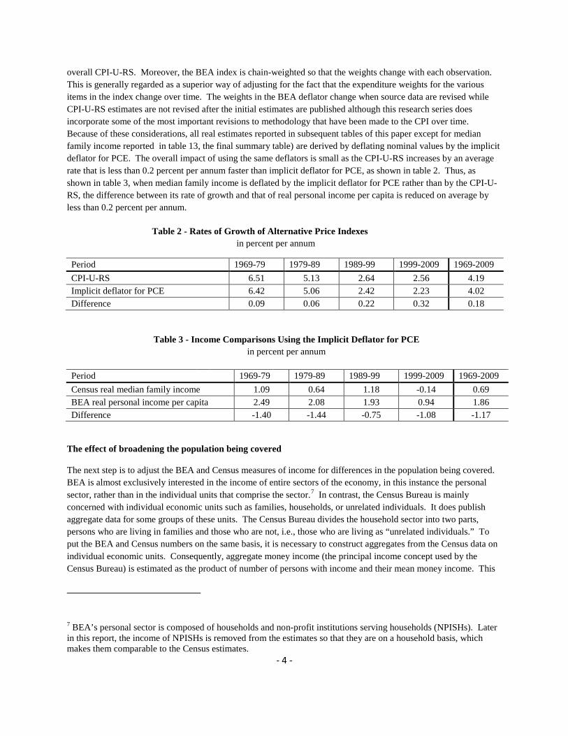
Table 6 compares the growth rates of real mean family income with those of real money income per capita. The latter measure increased much faster than the former from 1969 to 1989; since then the two series have increased at approximately the same rate. The reason for this difference in growth paths is that the share of total money income accounted by family income has declined substantially over time, see chart 1. Before any judgment can be made on the importance of these trends, it is necessary to examine the data a little more closely and determine what is causing them.

- 6 -

Table 6 - Real Mean Family Income and Real Money Income Per Capita in percent per annum

Period 1969-79 1979-89 1989-99 1999-2009 1969-2009 Real mean family income 1.25 1.27 1.73 0.06 1.08 Real money income per capita 2.44 1.85 1.71 0.07 1.51 Difference -1.18 -0.58 0.02 -0.01 -0.43

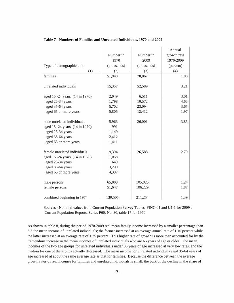
The fall in the share of aggregate money income accruing to families can be due to a decrease in the number of families relative to the number of unrelated individuals or a decrease in the mean family income relative to the mean income of unrelated individuals, or both. Table 7 shows that the number of families with income increased at annual rate of 1.08 percent from 1970 to 2009. During this period, the number of unrelated individuals increased at an annual rate of 3.21 percent, roughly triple the rate for families.

Table 7 breaks down the population of unrelated individuals into four age groups. Those aged 25-34 had the fastest rate of population growth. The oldest group, those aged 65 and above, had the slowest rate of growth as the share of unrelated individuals who are in this group declined. The number of unrelated related individuals who are men grew much faster than the number who are women. While men comprised only about 39 percent of unrelated individuals in 1970, they comprised over 49 percent of them in 2009. The number of women with income increased at faster rate than did the number of men as the labor force participation rate of women increased. By 2009 more women had income than did men.

70

80

90

100

1969 1974 1979 1984 1989 1994 1999 2004 2009

percent Chart 1 - Family Income as a Percent of

Money Income

family income as a percent of money income

- 7 -

Table 7 - Numbers of Families and Unrelated Individuals, 1970 and 2009

Annual

Number in Number in growth rate

1970 2009 1970-2009 Type of demographic unit

(thousands) (thousands) (percent)

(1)

(2) (3) (4) families

51,948 78,867 1.08

unrelated individuals

15,357 52,589 3.21

aged 15 -24 years (14 in 1970) 2,049 6,511 3.01 aged 25-34 years

1,798 10,572 4.65

aged 35-64 years

5,702 23,094 3.65 aged 65 or more years

5,805 12,412 1.97

male unrelated individuals

5,963 26,001 3.85

aged 15 -24 years (14 in 1970) 991 aged 25-34 years

1,149

aged 35-64 years

2,412 aged 65 or more years

1,411

female unrelated individuals 9,394 26,588 2.70 aged 15 -24 years (14 in 1970) 1,058 aged 25-34 years

649

aged 35-64 years

3,290 aged 65 or more years

4,397

male persons

65,008 105,025 1.24

female persons

51,647 106,229 1.87

combined beginning in 1974 130,505 211,254 1.39

Sources - Nominal values from Current Population Survey Tables FINC-01 and U1-1 for 2009 ; Current Population Reports, Series P60, No. 80, table 17 for 1970.

As shown in table 8, during the period 1970-2009 real mean family income increased by a smaller percentage than did the mean income of unrelated individuals; the former increased at an average annual rate of 1.10 percent while the latter increased at an average rate of 1.25 percent. This higher rate of growth is more than accounted for by the tremendous increase in the mean incomes of unrelated individuals who are 65 years of age or older. The mean incomes of the two age groups for unrelated individuals under 35 years of age increased at very low rates; and the median for one of the groups actually decreased. The mean income for unrelated individuals aged 35-64 years of age increased at about the same average rate as that for families. Because the difference between the average growth rates of real incomes for families and unrelated individuals is small, the bulk of the decline in the share of

- 8 -

total money income accruing to families is due to the fact that the number of unrelated individuals grew much faster than did the number of families.

Table 8 - Real Money Income of Families and Unrelated Individuals, 1970 and 2009

in constant 2005 dollars

Type of demographic unit

Real Mean

income in 1970

Real Mean

income in 2009

Annual growth

rate 1970-2009

(percent)

Real Median income in 1970

Real Median income in 2009

Annual growth

rate 1970-2009

(percent)

families

46,945 71,883 1.10 41,708 54,996 0.71

unrelated individuals

19,275 31,330 1.25 13,260 22,206 1.33

aged 15 -24 years (14 in 1970) 14,182 16,131 0.33 12,284 13,226 0.19

aged 25-34 years 30,811 33,280 0.20 28,828 27,809 -0.09 aged 35-64 years

24,676 37,603 1.09

aged 65 or more years

12,199 25,972 1.96 8,247 17,798 1.99

male unrelated individuals

24,897 34,984 0.88 19,191 25,096 0.69 aged 15 -24 years (14 in 1970) 15,116

13,285

aged 25-34 years

34,163

30,997 aged 35-64 years

31,060

aged 65 or more years

13,687

9,511

female unrelated individuals 15,708 27,757 1.47 10,496 19,602 1.61 aged 15 -24 years (14 in 1970) 13,307

11,269

aged 25-34 years

26,076

24,872 aged 35-64 years

19,756

aged 65 or more years

11,726

7,981

male persons

31,859 42,834 0.76 28,194 29,459 0.11 female persons

13,264 27,204 1.86 9,456 19,182 1.83

combined beginning in 1974 24,441 34,893 1.02 17,973 23,921 0.82

Sources - Nominal values from Current Population Survey Tables FINC-01 and U1-1 for 2009 ;

Current Population Reports, Series P60, No. 80, table 17 for 1970.

Table 8 also reveals that the increasing inequality that is found in the family income numbers is not found in the numbers for unrelated individuals. From 1970 to 2009 real median family income increased at an average annual rate of 0.71 percent, which is substantially less than the average annual rate of increase of 1.10 percent for mean family income. In contrast, the median income of unrelated individuals increased at an average annual rate that was actually greater than the average rate of increase in the mean income of these individuals.

- 9 -

For the period 1974 to 2009, table 8 also reports on the real income of persons, where the incomes of people who are in families and the incomes of unrelated individuals are combined in a single category. These numbers show that the real mean income of persons has increased at an average annual rate that is only slightly higher than the comparable rate for real median income. Note, however that the real incomes of females have increased by a much higher rate than have the incomes of males; the former increased at an average annual rate of 1.86 percent while the latter increased at an average annual rate of only 0.76 percent. Because the real median income for females increased at about the same rate as that for comparable mean, there was no increase in the inequality of incomes of females over this period. In contrast, the real median income for males increased at only an average annual rate of 0.11 percent. This rate is important for two reasons. Because it is so much lower than that for the comparable mean, it implies that there was a substantial increase in the inequality of incomes of males. Also, the rate is so low that had we used the CPI-U- RS for deflation rather than the implicit deflator for PCE, the resulting growth rate would have been negative. In sum, the falling share of aggregate money income accruing to families is largely the result of the large increase in the number of people living as unrelated individuals. Nevertheless, over the 39-year period, the mean income of unrelated individuals did increase at a faster rate than did the mean income of families. Another important trend was the convergence in incomes. Groups that had relatively low incomes in 1970, namely elderly unrelated individuals and women, experienced rates of income growth that were much higher than average. However, there was stagnation in the median incomes of groups that had relatively high incomes in 1970. The real median income of men hardly increased during the 39-year period while the real median income of younger unrelated individuals, those aged 25 to 34, actually fell. There also appeared to be an increasing inequality of incomes between families and between men.

Adjustments made for conceptual differences

There are important conceptual differences between BEA’s measure of real personal income and the Census Bureau’s measure of real money income. Many components of personal income are not included in money income. Conversely, a number of components of money income are not included in personal income. To a large extent, these differences occur because the measures have different orientations. Conceptually, personal income measures the income of the entire household sector and non-profit institutions serving households (NPISHs). Because of its macro orientation, BEA is able to measure the benefits that households receive from certain programs in terms of the costs of providing them (usually by employers or the government). It may be relatively easy to obtain data on the cost of an entire program, such as Medicare, while it would be very difficult to obtain information on the amount of benefits received by each individual family or person. Similarly, there are other areas where BEA is also able to use administrative data to measure income aggregates even when such data are not available at the level of individual households. Also, during the last few decades, BEA has not published data related to the distribution of income.

In contrast, the Census Bureau has a micro orientation. It is concerned with the incomes of individual families and persons as well as the distribution of income across all families and persons. It obtains its data by directly surveying individual households. Aggregate money income is obtained by summing up the individual money incomes of all families and unrelated individuals. Data on the provider’s costs of benefits that are received in kind may not be the most useful measure of the benefits received by an individual family.8 It is these differences in types

8 Measuring how much in kind benefits contribute to an individual’s income is extremely difficult. In some of its work on alternative measures of income, the Census Bureau measures the Medicare benefits received by an individual in terms of their “fungible value,” which assigns income to the extent that having the insurance would free up resources that would have been spent on medical care, see “Alternative Measures of Income Definitions” http://www.census.gov/hhes/www/income/data/historical/measures/redefs.html . Earlier attempts to value in-kind benefits received by individuals measured them in terms of their “cash-equivalent value,” a measure that was

- 10 -

of data sources that are responsible for most of the conceptual differences between the Census and BEA measures of household income.

This paper adjusts personal income by removing from it, wherever possible, those components that are not included in money income. Specifically, it removes those components for which a time series is found in the nearly 300 tables that comprise BEA’s National Income and Product Accounts. Estimates are also made for a few other adjustments that have very large values and for which underlying data are available. The needed adjustments that are not made because of the lack of data appear to have a relatively small total value. Likewise, this paper adjusts personal income by adding in a few components that are in money income but not in personal income. Here, adjustments are made where Census data exists over many decades so that a time series can be estimated.

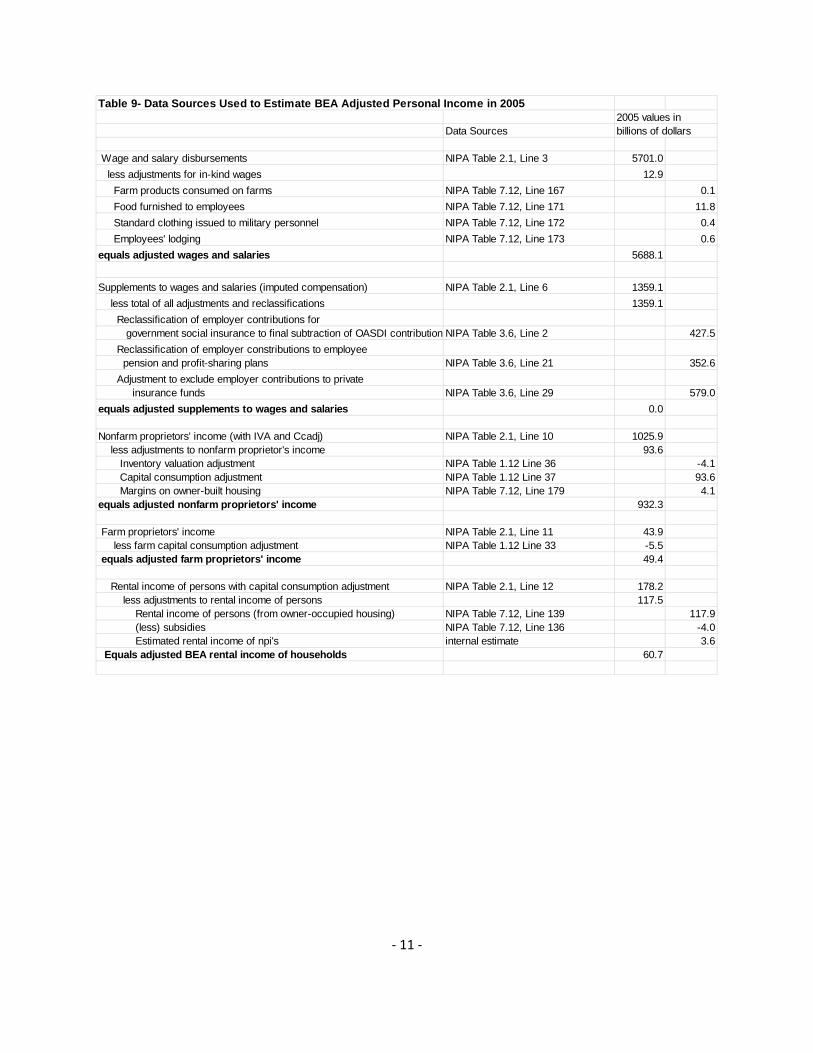
Most of the adjustments take various types of in-kind income out of personal income including: wages in kind, government transfers in kind, income from owner-occupied housing, unpaid banking services, and imputed interest from life insurance reserves. In addition, pensions are measured by benefits paid rather than by employer contributions to pension funds and the income earned on the plan assets (reserves) while employee contributions to social insurance are added back into personal income as they are in money income but not personal income. Adjustments are made to take out the income of non-profit institutions and to add in transfers between households. The values for the full set of adjustments are shown for 2005 in table 9. The adjustments are described in greater detail in an appendix to this paper.

thought to be theoretically attractive. For an early attempt to comprehensively define in-kind income and develop methodologies to measure its cash-equivalent value, see Gershon Cooper and Arnold J. Katz (1978).

- 11 -

Table 9- Data Sources Used to Estimate BEA Adjusted Personal Income in 20052005 values in

Data Sources billions of dollars

Wage and salary disbursements NIPA Table 2.1, Line 3 5701.0 less adjustments for in-kind wages 12.9 Farm products consumed on farms NIPA Table 7.12, Line 167 0.1 Food furnished to employees NIPA Table 7.12, Line 171 11.8 Standard clothing issued to military personnel NIPA Table 7.12, Line 172 0.4 Employees' lodging NIPA Table 7.12, Line 173 0.6equals adjusted wages and salaries 5688.1

Supplements to wages and salaries (imputed compensation) NIPA Table 2.1, Line 6 1359.1 less total of all adjustments and reclassifications 1359.1 Reclassification of employer contributions for government social insurance to final subtraction of OASDI contributionsNIPA Table 3.6, Line 2 427.5 Reclassification of employer constributions to employee pension and profit-sharing plans NIPA Table 3.6, Line 21 352.6 Adjustment to exclude employer contributions to private insurance funds NIPA Table 3.6, Line 29 579.0equals adjusted supplements to wages and salaries 0.0

Nonfarm proprietors' income (with IVA and Ccadj) NIPA Table 2.1, Line 10 1025.9 less adjustments to nonfarm proprietor's income 93.6 Inventory valuation adjustment NIPA Table 1.12 Line 36 -4.1 Capital consumption adjustment NIPA Table 1.12 Line 37 93.6 Margins on owner-built housing NIPA Table 7.12, Line 179 4.1equals adjusted nonfarm proprietors' income 932.3

Farm proprietors' income NIPA Table 2.1, Line 11 43.9 less farm capital consumption adjustment NIPA Table 1.12 Line 33 -5.5 equals adjusted farm proprietors' income 49.4

Rental income of persons with capital consumption adjustment NIPA Table 2.1, Line 12 178.2 less adjustments to rental income of persons 117.5 Rental income of persons (from owner-occupied housing) NIPA Table 7.12, Line 139 117.9 (less) subsidies NIPA Table 7.12, Line 136 -4.0 Estimated rental income of npi's internal estimate 3.6 Equals adjusted BEA rental income of households 60.7

- 12 -

Table 9 continued

BEA Personal income receipts on assets (dividends and interest) NIPA Table 2.1, Line 13 1542.0 less adjustments and reclassifications to income receipts on assets 903.4 Adjustment for imputed interest received by households NIPA Table 7.11, Line 61 374.3 Reclassification of return on pension reserves to pension income Uses rate on insurance reserves

and flow of funds outstandings 483.9 Adjustment for interest income of npi's NIPA Table 2.9, Line 50 28.9 Adjustment for dividend income of npi's NIPA Table 2.9, Line 51 16.3 equals adjusted interest and dividend income of households 638.6

Income from pensions 0.0 plus income from pensions found in other parts of personal income 836.5 Property income of plans (reclassified from income receipts on assets) From above 483.9 Employer contributions to employee pension and profit-sharing plans (reclassified from supplements to wages and salaries) From above 352.6 less adjustment for difference between benefits paid by employee pension (and profit sharing plans) and pension income in personal income 200.8adjusted pension income (equals benefits paid by plans) NIPA Table 6.11D, Line 38 635.7

Government social benefits to persons NIPA Table 2.1, Line 17 1482.7 less adjustment to exclude transfers in-kind 730.1 Hospital and supplementary medical insurance NIPA Table 3.12, Line 6 331.9 Military medical insurance NIPA Table 3.12, Line 16 2.1 Supplemental Nutrition Assistance Program (SNAP) NIPA Table 3.12, Line 21 29.5 Earned income credit NIPA Table 3.12, Line 25 49.2 Medical care NIPA Table 3.12, Line 32 315.0 Energy assistance NIPA Table 3.12, Line 38 2.4 less adjustment to exclude transfers from government to npi's NIPA Table 2.9, Line 53 17.4equals adjusted tranfer income 735.2

Other current transfer receipts, from business (net) NIPA Table 2.1, Line 24 25.8 less adjustment to exclude receipts from business transfers to persons they are not in money income 25.8Adjusted transfer receipts from business 0.0

Other transfer income items are already in personal income 0.0 Plus adjustments to put personal income on a household basis 51.2 plus transfers from npi's to households NIPA Table 2.9, Line 32 66.2 less transfers from business to npi's NIPA Table 2.9, Line 54 15.0Other npi income in adjusted personal income 51.2

Contributions for government social insurance, domestic NIPA Table 2.1, Line 25 -872.7 (these are a subtraction in the estimation of personal income) Plus sum of reclassifications and adjustments for contributions 872.7 Employer contributions for government social insurance NIPA Table 3.6, Line 2 (reclassified from supplements to wages and salaries) from above 427.5 Adjustment to include employee and self-employed contributions NIPA Table 3.6, Line 20 445.2 Adjusted contributions for government social insurance 0.0

Intrasector transfers there are none in personal income 0.0 Plus adjustment for intrasector transfers in money income 43.5 Child Support From Current Population Survey 26.0 Alimony From Current Population Survey 5.2 Financial assistance from Outside the household From Current Population Survey 12.2equals adjusted income from intrasector transfers 43.5

Personal Income NIPA Table 2.1, Line 1 10485.9Adusted personal income Sum of components given above 8834.7

- 13 -

The magnitude of the adjustments

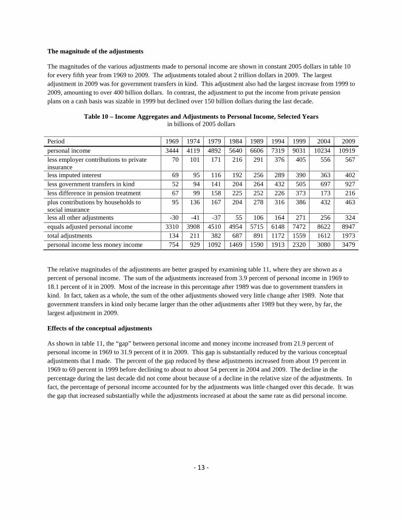
The magnitudes of the various adjustments made to personal income are shown in constant 2005 dollars in table 10 for every fifth year from 1969 to 2009. The adjustments totaled about 2 trillion dollars in 2009. The largest adjustment in 2009 was for government transfers in kind. This adjustment also had the largest increase from 1999 to 2009, amounting to over 400 billion dollars. In contrast, the adjustment to put the income from private pension plans on a cash basis was sizable in 1999 but declined over 150 billion dollars during the last decade.

Table 10 – Income Aggregates and Adjustments to Personal Income, Selected Years in billions of 2005 dollars

Period 1969 1974 1979 1984 1989 1994 1999 2004 2009 personal income 3444 4119 4892 5640 6606 7319 9031 10234 10919 less employer contributions to private insurance

70 101 171 216 291 376 405 556 567

less imputed interest 69 95 116 192 256 289 390 363 402 less government transfers in kind 52 94 141 204 264 432 505 697 927 less difference in pension treatment 67 99 158 225 252 226 373 173 216 plus contributions by households to social insurance

95 136 167 204 278 316 386 432 463

less all other adjustments -30 -41 -37 55 106 164 271 256 324 equals adjusted personal income 3310 3908 4510 4954 5715 6148 7472 8622 8947 total adjustments 134 211 382 687 891 1172 1559 1612 1973 personal income less money income 754 929 1092 1469 1590 1913 2320 3080 3479

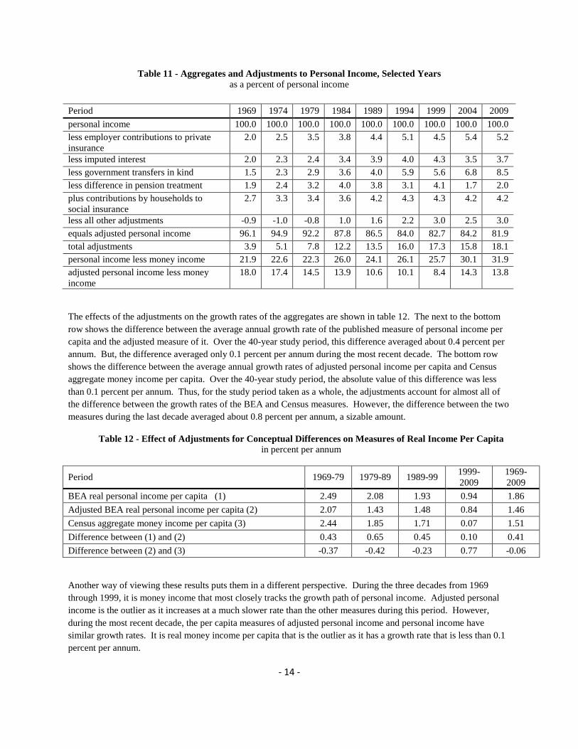
The relative magnitudes of the adjustments are better grasped by examining table 11, where they are shown as a percent of personal income. The sum of the adjustments increased from 3.9 percent of personal income in 1969 to 18.1 percent of it in 2009. Most of the increase in this percentage after 1989 was due to government transfers in kind. In fact, taken as a whole, the sum of the other adjustments showed very little change after 1989. Note that government transfers in kind only became larger than the other adjustments after 1989 but they were, by far, the largest adjustment in 2009.

Effects of the conceptual adjustments

As shown in table 11, the “gap” between personal income and money income increased from 21.9 percent of personal income in 1969 to 31.9 percent of it in 2009. This gap is substantially reduced by the various conceptual adjustments that I made. The percent of the gap reduced by these adjustments increased from about 19 percent in 1969 to 69 percent in 1999 before declining to about to about 54 percent in 2004 and 2009. The decline in the percentage during the last decade did not come about because of a decline in the relative size of the adjustments. In fact, the percentage of personal income accounted for by the adjustments was little changed over this decade. It was the gap that increased substantially while the adjustments increased at about the same rate as did personal income.

- 14 -

Table 11 - Aggregates and Adjustments to Personal Income, Selected Years as a percent of personal income

Period 1969 1974 1979 1984 1989 1994 1999 2004 2009 personal income 100.0 100.0 100.0 100.0 100.0 100.0 100.0 100.0 100.0 less employer contributions to private insurance

2.0 2.5 3.5 3.8 4.4 5.1 4.5 5.4 5.2

less imputed interest 2.0 2.3 2.4 3.4 3.9 4.0 4.3 3.5 3.7 less government transfers in kind 1.5 2.3 2.9 3.6 4.0 5.9 5.6 6.8 8.5 less difference in pension treatment 1.9 2.4 3.2 4.0 3.8 3.1 4.1 1.7 2.0 plus contributions by households to social insurance

2.7 3.3 3.4 3.6 4.2 4.3 4.3 4.2 4.2

less all other adjustments -0.9 -1.0 -0.8 1.0 1.6 2.2 3.0 2.5 3.0 equals adjusted personal income 96.1 94.9 92.2 87.8 86.5 84.0 82.7 84.2 81.9 total adjustments 3.9 5.1 7.8 12.2 13.5 16.0 17.3 15.8 18.1 personal income less money income 21.9 22.6 22.3 26.0 24.1 26.1 25.7 30.1 31.9 adjusted personal income less money income

18.0 17.4 14.5 13.9 10.6 10.1 8.4 14.3 13.8

The effects of the adjustments on the growth rates of the aggregates are shown in table 12. The next to the bottom row shows the difference between the average annual growth rate of the published measure of personal income per capita and the adjusted measure of it. Over the 40-year study period, this difference averaged about 0.4 percent per annum. But, the difference averaged only 0.1 percent per annum during the most recent decade. The bottom row shows the difference between the average annual growth rates of adjusted personal income per capita and Census aggregate money income per capita. Over the 40-year study period, the absolute value of this difference was less than 0.1 percent per annum. Thus, for the study period taken as a whole, the adjustments account for almost all of the difference between the growth rates of the BEA and Census measures. However, the difference between the two measures during the last decade averaged about 0.8 percent per annum, a sizable amount.

Table 12 - Effect of Adjustments for Conceptual Differences on Measures of Real Income Per Capita in percent per annum

Period 1969-79 1979-89 1989-99 1999-2009

1969-2009

BEA real personal income per capita (1) 2.49 2.08 1.93 0.94 1.86 Adjusted BEA real personal income per capita (2) 2.07 1.43 1.48 0.84 1.46 Census aggregate money income per capita (3) 2.44 1.85 1.71 0.07 1.51 Difference between (1) and (2) 0.43 0.65 0.45 0.10 0.41 Difference between (2) and (3) -0.37 -0.42 -0.23 0.77 -0.06

Another way of viewing these results puts them in a different perspective. During the three decades from 1969 through 1999, it is money income that most closely tracks the growth path of personal income. Adjusted personal income is the outlier as it increases at a much slower rate than the other measures during this period. However, during the most recent decade, the per capita measures of adjusted personal income and personal income have similar growth rates. It is real money income per capita that is the outlier as it has a growth rate that is less than 0.1 percent per annum.

- 15 -

This suggests a need to look a little more closely at the results for the most recent decade. The results are graphically portrayed in chart 2. They show that the pattern for real adjusted personal income per capita closely follows the pattern for the unadjusted measure. The pattern for real money income per capita is very different.

Comparison of major components

The last avenue of potential differences between the BEA and Census measures of household income that I will explore are those where, for a given component of aggregate income, differences remain after adjusting for conceptual differences between the measures. Some of these remaining differences may be due to measurement problems that lead to over- or under-reporting by households. Many types of income tend to be severely under-reported on income tax returns. Because of this, BEA adjusts reported estimates of certain types of income (such as proprietors’ income) up by a factor that reflects how much under-reporting there has been in the past. It is highly likely that the amount of misreporting will differ by type of income and that other factors may also be important. It is, therefore, imperative that we compare the adjusted BEA and Census measures for each specific component of income.

Beginning in 1994, detailed data exists on the components of money income on a consistent basis.9 For our purposes, it is useful to examine data on the five largest income components: wages and salaries, nonfarm proprietors’ income, interest and dividend income, pension benefits received, and (government) transfer payments

9 Similar data exists for earlier years but it is not as detailed, has some gaps, and is subject to changes in underlying definitions and coverage. Because we are primarily concerned with the period beginning in 1999, it is not necessary and probably preferable to avoid examining data on income components for earlier periods.

20,000

25,000

30,000

35,000

40,000

1999 2001 2003 2005 2007 2009

2005 dollars

Chart 2 - Adjusted and Unadjusted Measures of Real Personal Income Per Capita

real personal income per capitareal aggregate money income per capitaadjusted real personal income per capita

- 16 -

received. These components will be examined both in terms of percent differences as well as differences in their levels.

Chart 3 presents the differences between the Census and BEA estimates of comparable components; they are shown as percentages of the BEA estimates. All of the BEA components are measures that have been adjusted to remove the conceptual differences noted earlier in this paper. Any large differences in relative measurement error should be noticeable here. All of the five major components appear to have percent differences that increased in magnitude during the period shown. The percentage differences for wages and transfer payments are very small. The percentage differences for nonfarm proprietors’ income and pension benefits are quite large, but show little increase over the decade. The percentage differences for interest and dividend income are large and quite erratic. This difference declines sharply from 54 percent in 1994 to a negative value in 1999 and then rebounds sharply to 62 percent by 2002 before increasing to 75 percent in 2008.

Chart 4 presents the various series shown in chart 3. Here, however, they are shown here in terms of their dollar levels. This chart is particularly useful as it shows how much each component is contributing to the overall difference between the Census and adjusted BEA measures. The chart shows that for the period 1999 through 2009, there is relatively little increase in the magnitude of the difference between the adjusted BEA and Census measures for three components: wages and salaries, transfer payments, and non-farm proprietors’ income. However, the difference between the values of pension benefits received reported in the two measures increases dramatically- from about $200 billion in 1999 to about $500 billion in 2009. As before, the pattern for interest and dividend income stands out. The difference between the BEA and Census measures for this component was negative in 1999 but increased to about $824 billion in 2008 before declining to $370 billion in 2009.

-20.0

0.0

20.0

40.0

60.0

80.0

1994 1996 1998 2000 2002 2004 2006 2008

percent

Chart 3 - Difference Between Adjusted BEA and CPS Measures of Components of Household

Income, as a Percent of the BEA Measure

Wages and salariesNonfarm proprietors' incomeInterest and dividendsPension benefits received

- 17 -

The singular pattern for interest and dividend income suggests a need to investigate its causes. This is done with aid of chart 5, which compares the Census measure of this income with the adjusted and unadjusted BEA measures of it. The bulk of the adjustments to interest and dividend income are for imputed interest and the estimated property income on pension reserves owned by households. The chart shows that the adjustment lowers the unadjusted BEA measure by about 50 percent. Remarkably, the adjusted BEA measure of dividend and interest income has roughly the same time pattern as the unadjusted BEA measure. The Census measure of interest and dividend income has a completely different pattern. It is very cyclical and shows at best only a small upward trend.

-200-100

0100200300400500600700800900

1994 1996 1998 2000 2002 2004 2006 2008

billions of dollars

Chart 4 - Difference Between BEA and CPS Measures of Components of Household Income

Wages and salariesNonfarm proprietors' incomeInterest and dividendsPension benefits received

0200400600800

10001200140016001800200022002400

1994 1996 1998 2000 2002 2004 2006 2008

billions of dollars Chart 5 - Relationship Between BEA and Census Measures

of Interest and Dividend Income of Persons

BEA unadjusted interest and dividend incomeBEA adjusted interest and dividend incomeCensus interest and dividend income

- 18 -

At this point it seems evident that it is mostly the difference between the values of the BEA and Census measures of interest and dividend income over the last decade that explains why real per capita person income has increased over this period while real per capita money income has declined. To get further insight into what may have caused this divergence in values, it is useful to compare the estimates of interest and dividend income received by households from these two sources with data reported on individual income tax return. This is done on chart 6. Here the IRS measure not only includes dividend and interest income reported as part of adjusted gross income but also includes non-taxable interest income reported on the returns. For the most part, the Census measure closely follows the time path of the IRS measure, although at a lower level. Neither shows much growth over the entire period.

Other statistical sources are not very different from the Census growth patterns. The Consumer Finance Survey, which is sponsored by the Federal Reserve Board, reported that the percent of household income resulting from the receipt of interest and dividends increased from 4.8 percent in 1998 to only 5.2 percent in 2007. This is consistent with only a modest increase in these types of income. Similarly, Congressional Budget Office (CBO) data show that interest and dividends increased from 4.9 percent of pretax income in 1999 to 5.2 percent of it in 2007.

This leaves the question of what accounts for the tremendous surge in interest and dividend income that is part of adjusted personal income. Because of the lack of necessary underlying data, a complete answer to this question is not possible. Partial data do suggest what a sizable part of the answer may be. During the past decade there has been a tremendous growth in two relevant parts of capital income: profit distributions of S corporations and partnership income. The former is in personal income as is part of the latter, i.e., the property income of non-financial partnerships. The former increased by somewhat less than $200 billion during the past decade. The latter is very hard to estimate but data from the IRS indicate that portfolio income from income and dividends that was directly distributed to partners increased by about $263 billion from 1999 to 2008. These increases do not appear to be reflected in the Census measure of money income. This may reflect the fact that, as shown in CBO data, most of this income is received by households in the upper 1 percent of the income distribution.

0

200

400

600

800

1000

1200

1999 2001 2003 2005 2007 2009

billions of dollars

Chart 6 - Interest and Dividend Income of Households

Values on individual income tax returnsValues in CPS money incomeValues in adjusted personal income

- 19 -

Summary and Conclusion

During the period 1969 to 2009, the growth rates for the Census Bureau’s measure of real median family income and BEA’s measure of real per capita personal income are very different. Table 13 shows how much of the difference between these growth rates can be attributed to a number of factors. The use of the implicit deflator for PCE rather than the CPI-U-RS increases the growth rate on average by 0.17 percentage points during this period. Most of this effect occurred after 1989. Measuring family income by means rather than medians increased the average growth rate by another 0.39 percentage points as increasing inequality of incomes caused means to increase faster than medians. Broadening the population covered to include the incomes of unrelated individuals added another 0.43 percentage points to the average growth. Note, however, that almost all of the effects of this broadening on the average rate of growth were felt prior to 1990. Adjustments made to the BEA measure of personal income to make it conceptually similar to the Census measure of money income reduced the growth rate of former on average by 0.41 percentage points. But, they had very little effect on the rate of growth of personal income during the period 1999 to 2009. The remaining differences between the growth rates can be described as being due to unexplained measurement error. Surprisingly, for the entire 40-year period taken as a whole, this unexplained error is negligible. However, it is substantial on a decade by decade basis. In particular, during the period 1999 to 2009 it accounted for 0.77 percentage points of the average growth rate.

Table 13 - Summary of Effects of All Factors on the Growth Rate of Real Income Per Capita in percent per annum

Period 1969-79 1979-89 1989-99 1999-2009

1969-2009

Real median family income 1.01 0.58 0.96 -0.45 0.52 plus use of implicit deflator for PCE 0.09 0.06 0.22 0.31 0.17 plus use of mean rather than median family income 0.16 0.63 0.55 0.20 0.39

plus use of broader population measure 1.18 0.58 -0.02 0.01 0.43 plus unexplained measurement error -0.37 -0.42 -0.23 0.77 -0.06 plus conceptual adjustments to CPS basis 0.43 0.65 0.45 0.10 0.41 equals BEA real personal income per capita 2.49 2.08 1.93 0.94 1.86

During the period 1969 to 1999, most of the difference between the BEA and Census measures of income is due to demographic factors. Increasing income inequality between families caused median family income to increase much more slowly than mean family income. The share of household income accruing to families fell sharply. This fall was mostly due to an increase in the share of the population living as unrelated individuals and relatively large increases in the income of the elderly. Conceptual differences between the BEA and Census measures also played an important role in explaining the slower rate of growth of the Census measures. This was largely due to the sharp increases in the share of personal income in the form of in-kind transfers and employee benefits, both of which are not counted in the Census measure of money income.

During the period 1999 to 2009, neither demographic factors nor conceptual differences do much to explain the differences between the BEA and Census measures of household income. During this period, the effects of base broadening and the use of mean rather than median incomes increased the average growth rate of the Census measure by only 0.21 percent per annum. The conceptual adjustments made to real personal income per capita lowers its average rate of growth during this decade by only 0.10 percentage points. The end result is that there is a substantial unexplained gap. Adjusted real personal income per capita increases at an overage rate of 0.84 percent

- 20 -

per annum while the Census measure of real money income per capita increases at an average rate of only 0.07 percent per annum during this decade. Examination of the differences by income component reveals that most of the increase is concentrated in two components – property income and pension payments received. So far, a complete explanation for this has proved elusive. Nevertheless, there is some data that suggests that the divergence in measures of income from capital may have been caused, in part, by the large increase in income from S corporations and partnerships during the past decade.

References

Cooper, Gershon and Katz, Arnold J. 1978. The Cash Equivalent of In-Kind Income. Springfield, Va.: National Technical Information Service, April, Accession No. PB 276-767. Congressional Budget Office. 2008. “Historical Effective Tax Rates, 1979 to 2005: Supplement with Additional Data on Sources of Income and High-Income Households. December. Henry, Eric L., and Day, Charles. 2005. “A Comparison of Income Concepts: IRS Statistics of Income, Census Current Population Survey, and the BLS Consumer Expenditure Survey.” IRS Methodology Report series, Special Studies in Federal Tax Statistics, 149-157. Labonte, Marc. 2006. “Why has Household Income Fallen in the Current Expansion While GDP Has Risen?” CRS Report for Congress – from the CRS Web. Updated August 30. Order Code RL33519. Congressional Research Service.

Ruser, John; Pilot, Adrienne; and Nelson, Charles. 2004. “Alternative Measures of Household Income: BEA Personal Income, CPS Money Income, and Beyond.” Prepared for presentation to the Federal Economic Statistics Advisory Committee on December 14, 2004.

Ryscavage, Paul. 1986. “Reconciling Divergent Trends in Real Income.” Monthly Labor Review, July, 24-29.

Ryscavage, Paul. 1989. “Understanding real income trends: an analysis of conflicting signals,” Business Economics, 24 (1), 36-42.

Weinberg, Daniel H., 2004. “Income Data Quality Issues in the Annual Social and Economic Supplement to the Current Population Survey.” Prepared for American Enterprise Institute-University of Maryland Seminar on Poverty Measurement, October 12, 2004.

Weinberg, Daniel H.; Nelson, Charles T.; Roemer, Marc I.; and Welniak, Edward J. Jr. 1999. “Fifty Years of U.S. Income Data from the Current Population Survey: Alternatives, Trends, and Quality.” American Economic Review, 89 (2), 18-22.

Wheaton, Laura. 2007. “Underreporting of Means-Tested Transfer Programs in the CPS and SIPP,” 2007 Proceedings of the American Statistical Association, Social Statistics Section [CD-ROM], Alexandria, VA: American Statistical Association: 3622-3629.

- 21 -

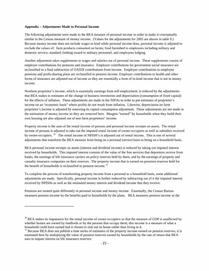
Appendix – Adjustments Made to Personal Income

The following adjustments were made to the BEA measure of personal income in order to make it conceptually similar to the Census measure of money income. (Values for the adjustments for 2005 are shown in table 9.) Because money income does not include wages in kind while personal income does, personal income is adjusted to exclude the values of: farm products consumed on farms; food furnished to employees including military and domestic service; standard clothing issued to military personnel; and employees lodging.

Another adjustment takes supplements to wages and salaries out of personal income. These supplements consist of employer contributions for pensions and insurance. Employer contributions for government social insurance are reclassified to a final subtraction of OASDI contributions from income. Employer contributions to employee pensions and profit-sharing plans are reclassified to pension income. Employer contributions to health and other forms of insurance are adjusted out of income as they are essentially a form of in-kind income that is not in money income.

Nonfarm proprietor’s income, which is essentially earnings from self-employment, is reduced by the adjustments that BEA makes to estimates of the change in business inventories and depreciation (consumption of fixed capital) for the effects of inflation. These adjustments are made in the NIPAs in order to put estimates of proprietor’s income on an “economic basis” where profits do not result from inflation. Likewise, depreciation on farm proprietor’s income is adjusted by removing its capital consumption adjustment. These adjustments are not made in the estimation of money income so they are removed here. Margins “earned” by households when they build their own housing are also adjusted out of non-farm proprietors’ income.

Property income is the sum of the rental income of persons and personal income receipts on assets. The rental income of persons is adjusted to take out the imputed rental income of owner-occupiers as well as subsidies received by owner-occupiers. 10 The rental income of NPISH’s is adjusted out of rental income. This is one of several adjustments that transform the BEA measure from being on a personal (sector) basis to being on a household basis.

BEA personal income receipts on assets (interest and dividend income) is reduced by taking out imputed interest received by households. This imputed interest consists of the value of the free services that depositors receive from banks, the earnings of life insurance carriers on policy reserves held by them, and by the earnings of property and casualty insurance companies on their reserves. The property income that is earned on pensions reserves held for the benefit of households is reclassified to pension income.11

To complete the process of transforming property income from a personal to a household basis, some additional adjustments are made. Specifically, personal income is further reduced by subtracting out of it the imputed interest received by NPISHs as well as the estimated money interest and dividend income that they receive.

Pensions are treated quite differently in personal income and money income. Essentially, the Census Bureau measures pension income by the benefits paid to households by the plans. BEA measures pension income as the

10 BEA makes its imputation for the rental income of owner-occupiers so that the measure of GDP is unaffected by whether homes are owned by landlords or by the persons that occupy them; this income is a measure of what a household could have earned had it chosen to rent out its home rather than living in it. 11 Because BEA does not publish a time series of estimates of the property income earned on pension reserves, it is estimated here by multiplying the value of pension reserves owned by households by the rate of return that BEA uses to impute interest on life insurance reserves.

- 22 -

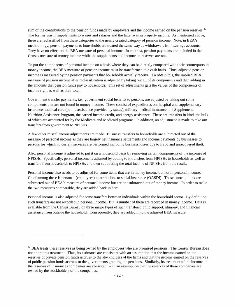
sum of the contributions to the pension funds made by employers and the income earned on the pension reserves.12 The former was in supplements to wages and salaries and the latter was in property income. As mentioned above, these are reclassified from these categories to the newly created category of pension income. Note, in BEA’s methodology, pension payments to households are treated the same way as withdrawals from savings accounts. They have no effect on the BEA measure of personal income. In contrast, pension payments are included in the Census measure of money income while the supplements and income on reserves are not.

To put the components of personal income on a basis where they can be directly compared with their counterparts in money income, the BEA measure of pension income must be transformed to a cash basis. Thus, adjusted pension income is measured by the pension payments that households actually receive. To obtain this, the implied BEA measure of pension income after reclassification is adjusted by taking out all of its components and then adding in the amounts that pension funds pay to households. This set of adjustments gets the values of the components of income right as well as their total.

Government transfer payments, i.e., government social benefits to persons, are adjusted by taking out some components that are not found in money income. These consist of expenditures on: hospital and supplementary insurance, medical care (public assistance provided by states), military medical insurance, the Supplemental Nutrition Assistance Program, the earned income credit, and energy assistance. These are transfers in kind, the bulk of which are accounted for by the Medicare and Medicaid programs. In addition, an adjustment is made to take out transfers from government to NPISHs.

A few other miscellaneous adjustments are made. Business transfers to households are subtracted out of the measure of personal income as they are largely net insurance settlements and income payments by businesses to persons for which no current services are performed including business losses due to fraud and unrecovered theft.

Also, personal income is adjusted to put it on a household basis by removing certain components of the incomes of NPISHs. Specifically, personal income is adjusted by adding to it transfers from NPISHs to households as well as transfers from households to NPISHs and then subtracting the total income of NPISHs from the result.

Personal income also needs to be adjusted for some items that are in money income but not in personal income. Chief among these is personal (employees) contributions to social insurance (OASDI). These contributions are subtracted out of BEA’s measure of personal income but are not subtracted out of money income. In order to make the two measures comparable, they are added back in here.

Personal income is also adjusted for some transfers between individuals within the household sector. By definition, such transfers are not recorded in personal income. But, a number of them are recorded in money income. Data is available from the Census Bureau on three major types of such transfers: child support, alimony, and financial assistance from outside the household. Consequently, they are added in to the adjusted BEA measure.

12 BEA treats these reserves as being owned by the employees who are promised pensions. The Census Bureau does not adopt this treatment. Thus, its estimates are consistent with an assumption that the income earned on the reserves of private pension funds accrues to the stockholders of the firms and that the income earned on the reserves of public pension funds accrues to the governments granting the pensions. Similarly, its treatment of the income on the reserves of insurances companies are consistent with an assumption that the reserves of these companies are owned by the stockholders of the companies.