Explaining Movements in the Labor Share1

Samuel Bentolilacemfi and cepr

Gilles Saint-PaulUniversitat Pompeu Fabra and cepr

This version: April 1999

1We are very grateful to Manuel Arellano for much helpful advice. We wish to thankBrian Bell for supplying us with the CEP-OECD Data Set and Steve Bond for help withDPD98. A preliminary version of this paper was circulated and presented at the MITInternational Economics Seminar in March 1995, while Saint-Paul was visiting the MITEconomics Department. We are grateful to participants at that workshop and to those atCREST, the Madrid Macroeconomics Workshop (MadMac), Universitat Pompeu Fabraand Université de Toulouse for their helpful comments.

Abstract

In this paper we study the evolution of the labor share in the OECD since 1970.We show it is essentially related to the capital-output ratio; that this relationshipis shifted by factors like the price of imported materials or the skill mix; and thatdiscrepancies between the marginal product of labor and the real wage (due to,e.g., product market power, union bargaining, and labor adjustment costs) causedepartures from it. We provide estimates of the model with panel data on 14industries and 14 countries for 1973-93 and use them to compute the evolution ofthe wage gap in Germany and the US.

Jel classification. E25, J30.Key words: Labor share, capital-output ratio.

1 Introduction

In this paper we explore the factors driving the observed movements in the laborshare in OECD countries from 1970 to now. The labor share does not very oftengenerate an interest among neoclassical economists, partly because its constancyis taken as a granted ”stylized fact of growth”.1 On the other hand, the laborshare is very much present in the political debate as a measure of how the ”bene…tsof growth” are shared between labor and capital. For example, its decline sincethe mid-1980s is often used by unions in Europe as an argument against policiesof wage moderation, and by governments in order to justify increased taxation ofpro…ts. Moreover, contrary to economists’ presumptions, there have been consid-erable medium-run movements in the labor share over a period of 35 years, asshown in Figures 1 to 4 for several countries. For these reasons, it is important tounderstand the determinants of the labor share, which is the purpose of this paper.

It is quite striking to …nd that there are large cross-country di¤erences in thebehavior of the labor share. The UK exhibits the closest approximation to the”growth stylized fact”, with the labor share experiencing large short-run ‡uctua-tions around a stable level (Figure 1). In the US it undergoes sizable short-run‡uctuations around a mild downward trend, becoming essentially ‡at in the 1980s(Figure 2). In Japan, on the contrary, it experiences a sharp rise, slowing downconsiderably after 1975 (Figure 3). The picture for continental Europe is typicallyhump-shaped, with the labor share going up and then down. But actual countryexperiences are heterogeneous: in Germany and France the labor share peaks inthe early 1980s (Figure 4), while in other countries like Italy, the Netherlands, andSpain it does so in the mid-1970s.

From a cross-country perspective, it should be noted that these large di¤er-ences across countries take place even though they are relatively similar from atechnological point of view. Table 1 shows the evolution of the labor share in thebusiness sector of 14 OECD countries since 1970. As evidenced by its …rst threecolumns, the labor share has not converged among these countries during the 1980s(the standard deviation has actually increased). In 1990, some countries like Fin-land, Sweden or the UK showed labor shares around 72%, while others like France,Germany or Italy had values around 62%.

In the policy debate, movements in the labor share are often interpreted aschanges in real wages. It is for example usually heard that because the labor shareis currently low in Europe, there is no real wage problem. But this is clearlymistaken, since it all depends on the elasticity of labor demand. The last twocolumns of Table 1 suggest that the correlation between changes in wages andchanges in the labor share is not tight (in other words, labor productivity behaves

1Recent exceptions are Blanchard (1997,1998) and Caballero and Hammour (1998).

1

di¤erently across countries). For example, from 1970 to 1990 France had one ofthe sharpest drops in the labor share and an above-average increase in the averagereal wage, while Sweden had one of the largest increases in the labor share and oneof the lowest increases in real wages.2 Thus, there is no clear pattern, and a moresystematic exploration of the determinants of the labor share is called for.

What can we learn from analyzing the labor share? First of all, it leads to adi¤erent approach to the study of labor demand. The traditional analysis of labordemand relates it to factors such as wages, labor-embodied technical progress, andcapital (or, alternatively, real interest rates). This type of analysis has often runinto trouble, e.g., in estimating the elasticity of labor demand with respect to thosefactors (see Hamermesh 1993). For some purposes, however, these estimates arenot needed, and the labor share provides a compact way of looking at labor demandwhich directly controls for the role of the above mentioned factors.

We shall show that, as long as labor is paid its marginal product, there shouldbe a one-for-one relationship between the labor share and the capital-output ratio,which we label the share-capital schedule. As long as that condition holds –and itmust, at least in long-run equilibrium–, changes in any of those three factors willgenerate changes of both the labor share and the capital-output ratio along thatschedule. Any change in the labor share which shows up as a deviation from thatrelationship must arise from a shift in labor demand which is not due to real wages,capital accumulation or technical progress, and therefore has to be explained byother considerations. In what follows, we study the role of factors which displacethe schedule, such as changes in the price of imported materials or in the skill mix,and those which put the economy o¤ the schedule, by changing the gap betweenthe shadow marginal cost of labor and the wage, such as changes in markups ofprices over marginal costs, union bargaining power, or labor adjustment costs.

This approach is motivated by an attempt to understand the causes of Europeanunemployment. It allows us to disentangle some of the factors that played a role inthe increase in unemployment. For example, excess wage growth must necessarilybe associated with movements along the share-capital relationship. Increases inunemployment that are associated with a shift in the position of that schedule, orthat put the economy o¤ that schedule, cannot be ascribed to just a wage push.

Our approach may then be used to interpret the observed movements in un-employment. We show that one way to do so is to compute the wage gap, i.e.the di¤erence between wages and the marginal product of labor at full employ-ment. In the literature it has often been concluded that wage gaps were high inEuropean economies in the second half of the 1970s –and this was associated withunemployment being Classical–, but had disappeared by the mid-1980s –so that

2The correlation coe¢cient between labor share changes and real wage changes over the period1970-90 across these 14 countries is 0.61.

2

unemployment had become Keynesian– (see Bean, 1994). Our model provides analternative way of computing and decomposing wage gaps, starting from estimatesof the labor share relationship. Under our interpretation, a low or negative wage gapassociated with high unemployment does not indicate a Keynesian disequilibriumbut rather a fall in labor demand that may be due to increased uncertainty, highermarkups, higher prices of imported materials, etc. Recently, Blanchard (1998) hasargued that the increase in European unemployment cannot be explained by laborsupply and user cost shifts alone, so that labor demand shifts are also a necessaryingredient. The model proposed in this paper analyzes the nature of the lattershifts, and our empirical estimates quantify and decompose them.

Given this aim, we analyze the empirical performance of the model, using paneldata on a sample of 14 industries in 14 OECD countries, over the period 1973-93.We estimate the relationship between the labor share and a number of its presumeddeterminants according to the model. In our estimation we follow Arellano andBover’s (1995) recent proposal of a system estimator for panel data, i.e. a gen-eralized method of moments estimator with instrumental variables which employsthe information contained in the relationship between the variables in both levelsand …rst di¤erences, which helps in raising the e¢ciency of the estimation. We…nd evidence in favor of an empirical relationship between the labor share and thecapital-output ratio, e.g. the share-capital relationship, but also signi…cant shiftsof the labor share coming from the real price of oil and from factors which cre-ate a wedge between the shadow marginal cost of labor and the wage, like laboradjustment costs and union bargaining power.

We then employ the empirical estimates in computing wage gaps in two largeeconomies, the US and Germany, and decompose their evolution according to thetheoretical model. The results from this exercise are striking. Only a small fractionof observed movements is the wage gap, whether in Germany or the US, can beattributed to labor-augmenting technical progress or changes in factor costs such aswages and interest rates. Most of those movements indicate shifts in labor demanddue to the gap between the shadow cost of labor and the wage. Furthermore,such movements are much more pronounced in Germany than in the US. Thisis in accordance with the view that some labor market rigidities (most notablyemployment protection legislation) are likely to increase the di¤erence between theshadow cost of labor and wages, and to make the former more volatile.

The paper is structured as follows. Section 2 presents a model of the determi-nation of the labor share. After introducing the stripped-down model, which yieldsthe key relationship between the labor share and the capital-output ratio, we showhow the relaxation of various assumptions may a¤ect such relationship. Section 3presents empirical evidence on the performance of the model on international paneldata. Section 4 exploits the empirical relationship to estimate and decompose wagegaps in Germany and the US. Section 5 contains our conclusions.

3

2 Theory

We start by sorting out, from an analytical point of view, the various factors whichmay explain variations in the labor share.

2.1 The labor share and the capital-output ratio

When trying to explain variations in the labor share we need to depart from theusual assumption of a Cobb-Douglas production function. We show that under theassumptions of constant returns to scale and labor embodied technical progress,there are strong restrictions on the behavior of the labor share, in the sense thatthere should be a one-for-one relationship between it and the capital-output ratio.

Proposition 1 Assume a constant returns to scale, di¤erentiable production func-tion by which output, Y , is produced with two factors of production, capital, K, andlabor, L, and labor-augmenting technical progress, B:

Y = F (K;BL)

Then, under the assumption that labor is paid its marginal product, there exists aunique function g such that:

sL = g (k) (1)

where sL ´ wL=(pY ) is the labor share, with w denoting the wage and p the productprice, and k ´ K=Y is the capital-output ratio.

Proof. Let us rewrite the production function as Y = Kf (BL=K) = Kf (l),where l ´ BL=K. In equilibrium we have:

w

p= Bf 0(l) (2)

where the prime denotes the …rst derivative, implying that the labor share is equalto:

sL =BLf 0(l)

Kf (l)=lf 0(l)

f(l)(3)

The capital-output ratio is then equal to:

k =1

f(l)(4)

Eliminating l between equations (3) and (4) we …nd a univariate relationship be-tween sL and k: q.e.d.

4

Proposition 1 tells us that even if the production function is not Cobb-Douglas,there is a stable relationship between the labor share and an observable variable, thecapital-output ratio. From now on, we shall refer to this relationship as the share-capital (SK) schedule (or curve). This relationship is unaltered by changes in factorprices –e.g. wages or interest rates– or quantities, or in labor-augmenting technicalprogress. That is to say, any change in the labor share which is triggered by thosefactors will be along that schedule, so that they cannot explain any deviation fromthe SK relationship, i.e. any residual in equation (1). Note that equations (1) and(3) are essentially the same relationship, but equation (1) is simpler to estimate,since it does not require the computation of l, which itself requires us to computeB, labor-augmenting technical progress.

Our aim is thus to decompose changes in the labor share between those ex-plained by the capital-output ratio –due to changes in factor prices and labor-augmenting technical progress– and those explained by the residual –i.e., due toother factors discussed below–.

To illustrate Proposition 1 more concretely, let us consider what happens whenthe production function has a constant elasticity of substitution (CES):

Y = ((AK)" + (BL)")1=" (5)

where A, B and " are technological parameters.In this case, the labor share is equal to:

sL =(BL)"

(AK)" + (BL)"(6)

while the capital-output ratio is simply equal to:

k =

ÃK"

(AK)" + (BL)"

!1="(7)

From equations (6) and (7) we have:

sL = 1¡ (Ak)" (8)

We therefore see that the relationship between sL and k is very simple in thiscase. It is monotonic in k; either increasing or decreasing depending on the signof ": if labor and capital are substitutes, a lower capital intensity will increase thelabor share, and conversely if they are complements. For more general productionfunctions, the relationship need not be monotonic, so that the labor share can goup and then down as some variable driving changes in k (such as real wages orinterest rates) varies.

5

2.2 Deviations from a stable SK relationship

We now analyze the factors that generate deviations from this simple relationship.To do so, let us …rst de…ne more precisely the SK curve in equation (1), as arelationship between k = 1=f (l) and ´ ´ lf 0(l)=f (l), the employment elasticity ofoutput. Then the economy is on the SK curve in the (k; sL) plane if and onlyif sL = ´, i.e. the marginal product of labor is equal to the real wage. We shalldistinguish between two types of deviations, depending on whether they cause shiftsof the SK curve, i.e. shifts in the g(:) function in equation (1), or movements o¤it, i.e. increases in the di¤erence between sL and ´.

First, the SK curve is stable if only labor-augmenting technical progress a¤ectsthe aggregate production function. Other factors a¤ecting it, such as A in equation(8) for the CES case, i.e. capital-augmenting technical progress, will shift the SKcurve if they are not constant. This is the …rst possible reason for not having astable one-to-one relationship between sL and k.

Second, there are factors which create a wedge between the real wage and themarginal product of labor. While they do not a¤ect the relationship between ´ andk, they create a gap between sL and ´. These factors therefore do not shift theSK curve, but put the economy o¤ that schedule in the (k; sL) plane. These threesources of movements are illustrated in Figure 5. Let us now discuss each type ofdeviation in detail.

2.3 Non-neutralities in the aggregate production function

We …rst discuss sources of deviations which shift the SK schedule by changing theaggregate production function in a non-labor-augmenting way. We consider twosources: imported materials and heterogeneity in the composition of the workforce.

2.3.1 Imported raw materials

What if there are imported raw materials whose price ‡uctuates? Unless very re-strictive conditions hold, these ‡uctuations will shift the SK schedule in a directionwhich will depend on the characteristics of the production function.

Let us assume that we have Y = F (K;BL;M), where M denotes importedraw materials (say oil), with price q. This can be rewritten as Y = Kf (l;m); withl ´ BL=K, as above, and m ´ M=K. L and M are set so as to maximize pro…ts.The …rst order conditions are:

Bf 01(l;m) =w

p; f 02(l;m) =

q

p(9)

Value added is de…ned as (see Bruno and Sachs 1985, Appendix 2B, for adiscussion): ~Y ´ Y ¡ (q=p)M , and the SK curve is now a relationship between

6

esL; the share of labor in value added given by esL ´ wL=(p ~Y ), and ~k ´ K= eY , thecapital-value added ratio. We now have, instead of (4):

~k =1

f(l;m)¡ qpm

(10)

implying:

esL =lf 01(l;m)

~k(11)

Equations (9) and (10) now de…ne l and m as functions of ~k and q=p. Pluggingthese into equation (11) we get a relationship where esL is a function not only of ~kbut also of q=p.

To get a grasp of the e¤ects at work when the labor share changes as q=pincreases, we can di¤erentiate equations (9) to (11), to get the change in the laborshare holding ~k constant:

desLd(q=p)

=1~k

Ãm+

lf 0012f 0022

+lm

f 01f0022

³f 0011f

0022 ¡ (f 0012)2

´!(12)

where f 0011f0022 ¡ (f 0012)2 > 0 is the Hessian of the production function.

The …rst term in the brackets of (12) is positive; it is due to the fact that tomaintain a constant ratio between capital and value added as materials prices rise,the labor-capital ratio must rise, which pushes the labor share upwards. The secondterm is typically negative as long as imported materials increase the marginalproduct of labor. It measures the fact that given l; imports fall when q=p increases,which reduces the marginal product of labor and therefore wages and the laborshare. The third term is also negative. It captures the fall in wages induced by therequired increase in the labor capital ratio (taking into account the indirect e¤ectof the induced e¤ect on m).

Thus, the price of imported materials shifts the SK schedule in an ambiguousdirection. To illustrate this, let us look again at the CES case. Assume the followingproduction function:

Y = ((AK)" + (BL)" + (CM)")1="

where A, B, C, and " are the technological parameters now. The correspondingexpression for the labor share is then:3

3The …rst-order condition for pro…t maximization with respect to M is:((AK)" + (BL)" + (CM)")

1="¡1C"M"¡1 = q=p. This equation can be solved for M; yielding:

M = C¡1³

(q=p)"=("¡1)

C"=("¡1)¡(q=p)"=("¡1)

´1="

((AK)" + (BL)")1=". Given the de…nition of value added we

7

esL = 1¡ (A=C)"³C

""¡1 ¡ (q=p) "

"¡1´"¡1 ~k" (13)

We can thus in principle take into account the impact of changes in the priceof imported materials on the labor share by estimating (13) or a linearized variantof it. Note that the SK schedule will shift upwards when q=p rises if and only if" > 0: The more labor is a substitute for capital, the lower the wage fall requiredto increase l so as to maintain ~k constant when imported materials fall, and thelarger the increase in the labor share.

2.3.2 Labor heterogeneity

Until now, we have assumed a homogenous labor force. Recently, considerableattention has been devoted to the changes in the returns to skills that have beenobserved in the US and other countries since the mid-1970s. These developmentsmay also have a¤ected the labor income share. Thus, we may …nd it worthwhile toextend our framework so as to distinguish between skilled and unskilled workers.We do so in this subsection, although our data does not allow us to implement sucha distinction in our empirical analysis.

How is the labor share a¤ected if there are several types of labor, say skilledand unskilled? In general, there will be again a breakdown in the SK scheduleas captured by equation (3). However, under some restrictions in the productionfunction, property (3) still holds. These restrictions are less strong, for example,than those needed for the price of materials not to a¤ect the residual.

Proposition 2 Assume there are three inputs, capital and two types of labor, L1and L2, and that the production function is given by:

Y = H (K;G(B1L1; B2L2))

where B1 and B2 are the respective technological parameters, and functions G (:; :)and H(:; :) are homogeneous of degree 1. Then there exists a one-to-one relationshipbetween sL and k:

sL = g (k)

where g only depends on H:

have: eY = C¡1 ((AK)" + (BL)")1=" ¡

C"=("¡1) ¡ (q=p)"=("¡1)¢ "¡1

" .The last term in brackets is decreasing in q=p and captures the e¤ect of the price of materials

on total factor productivity de…ned in terms of value added; it is multiplicative in output. Thesecond equation de…nes a functional form similar to equation (5) so that by making the appropriatesubstitutions in equation (8) we obtain equation (13).

8

Proof. The …rst-order conditions for maximization with respect to L1 and L2,with respective wages are w1 and w2, are:

@Y

@Li=wip= Bi

@H

@G

@G

@(BiLi); i = 1; 2

The labor share is then equal to:

sL =w1L1 + w2L2

pY=

2Pi=1

³BiLi

@H@G

@G@(BiLi)

´

H (K;G)=

G@H@G

H(K;G)= Á

µG

K

¶(14)

where we have used the homogeneity of G and H. The capital-output ratio is thensimply equal to K=H(K;G), which also only depends on G=K . Substituting intoequation (14) we may then …nd a relationship between sL and k. q.e.d.

Proposition 2 tells us that if skilled and unskilled labor enter production throughany aggregate function which is homogeneous of degree one, then there is still arelationship between the labor share and the capital-output ratio, and this rela-tionship is una¤ected by relative prices and relative factor supplies. Moreover, itis also una¤ected by any change in the relative demand for unskilled labor due totechnology, provided such change shows up in G, but not in H .4

It is however often argued (see, for example, Krusell et al. 1997) that thereis more complementarity between skilled labor and capital than between unskilledlabor and capital. In such case, we can show that the ratio of the wages of the twotypes of labor would enter the SK relationship (see Appendix A). Unfortunately,that ratio is not observed in our database, thus we will proceed under the workinghypothesis that Proposition 2 is valid.

2.4 Di¤erences between the marginal product of labor andthe real wage

We now turn to those factors that put the economy o¤ the SK curve by generatinga gap between the marginal product of labor and the real wage. We consider threeof them: product market power, union bargaining, and labor adjustment costs.

2.4.1 Variations in the markup

Assume …rms are imperfectly competitive, so that there is a markup ¹ of prices onmarginal costs. Accordingly, the optimality condition (2) should be replaced with:

4A particular example where Proposition 2 holds is a production function which isCES in capital and a labor aggregate, itself CES in skilled and unskilled labor: Y =³(AK)" + ((B1L1)

½ + (B2L2)½)

"=½´1="

. This production function includes, as a special case, a

CES in all three inputs (when ½ = "): Y = ((AK)" + (B1L1)" + (B2L2)

")1=".

9

@F

@L= Bf 0(l) = ¹

w

p

so that we now have:

sL = ¹¡1 lf

0(l)

f(l)= ¹¡1´

implying a relationship such as sL = ¹¡1g(k): Clearly, if the markup is constant,there should still be a stable relationship between sL and k. However, variationsin the markup will a¤ect that relationship and will show up in the ”residual”. Forexample, if markups are countercyclical, the labor share will tend to be procyclicalonce we have controlled for k:

Note that the above relationships are actually used by macroeconomists in orderto compute the markup (see Hall 1990; Rotemberg and Woodford 1991 and 1992;and Bénabou 1992). From our point of view, this is unfortunate: many deviationsof the labor share from the predicted SK schedule may be due to factors otherthan the markup. Ideally, one would want to correlate these deviations with directmeasures of the markup. In their survey paper on the cyclical behavior of markups,Rotemberg and Woodford (1997) actually discuss various sources of deviation. Forinstance, they comment on the inclusion of materials in the production function,but assume that materials are a …xed proportion of aggregate output.5

Recall now Figure 5, which summarizes the discussion up to this point. Itdepicts the SK curve in the (k; sL) plane, showing that increases in wages implymovements along the curve, but changes in the price of materials cause shifts ofthe curve itself, while variations in the markup put the economy o¤ the schedule.

2.4.2 Bargaining

Another source of deviations from the SK curve is the existence of bargainingbetween …rms and workers. Indeed, increases in the labor share are customar-ily interpreted as increases in workers’ bargaining power, and it is often hastilyconcluded that employment consequently has to decline. The issue is more compli-cated, though, because everything depends on what bargaining model is assumed.

Right to manage Under the right-to-manage model, …rms and unions …rst bar-gain over wages and then …rms set employment unilaterally, taking wages as given.This model is widely seen as a good description of how bargaining actually takes

5These authors also mention other deviations ignored here, like overhead labor, …xed costsin production, increasing marginal wages, or variable e¤ort. However, their paper’s focus ison the cyclicality of the markup, rather than on the shifts in labor demand and its e¤ects onunemployment, as ours.

10

place in many countries (see, e.g., Layard et al. 1991, chapter 2). But then, because…rms are wage takers when setting employment, the marginal product equation (2)remains valid, and so does Proposition 1. Under this model, changes in the bar-gaining power of workers may move the labor share, but along the SK curve, notaway from it, in a direction which depends on the elasticity of substitution betweenlabor and capital (see equation (8) for the CES case). More speci…cally, an increasein workers’ bargaining power creates a wage push that increases k as …rms substi-tute capital for labor. But the labor share may rise or fall depending on the slopeof the SK curve (i.e. the elasticity of substitution between labor and capital), andthe relationship between k and sL is una¤ected.

We can represent the right-to-manage model as follows. Wages are …rst set tomaximize the following Nash maximand:

maxw

³V ¤(w;K)¡ ¹V

´µ ³¦¤(w;K)¡ ¹¦

´1¡µ

where V ¤(w;K) and ¦¤(w;K) are reduced-form union utility and pro…ts, respec-tively, while ¹V and ¹¦ are the appropriate threat points. µ is a parameter weightingthe two objective functions, which can be labeled as union bargaining power. Inthe second stage of the game, the …rm determines employment by maximizing:

¦¤(w;K) = maxL

¦(w;L;K) = pF (K;BL)¡ wL

This de…nes an optimal employment level, L¤(K), a reduced form pro…t, ¦¤(w;K),and a reduced form utility, V ¤(w;K) = V (w;L¤(K)). Now, the …rst-order condi-tion for pro…t maximization is clearly (2), so that (3) and (4) are still valid. Thusthe relationship between sL and k is una¤ected by µ.6

E¢cient bargaining If, on the other hand, …rms and workers bargain over bothwages and employment, they will set employment in an e¢cient way, implying thatthe marginal product of labor is equal to its real opportunity cost ( ¹w=p):

Bf 0(l) =¹w

p

In the sort run, an increase in the bargaining power of workers does a¤ect thelabor share but is not re‡ected in employment. In the long-run, adjustment of thecapital stock indeed implies that changes in the bargaining power of workers alsoa¤ects employment.

6Here we have assumed that bargaining over wages takes place after the capital stock isdetermined. Our conclusions would be una¤ected if instead the capital stock was determined bythe …rm after wage setting, or even if bargaining took place over the capital stock, as long asemployment is determined by pro…t maximization given wages.

11

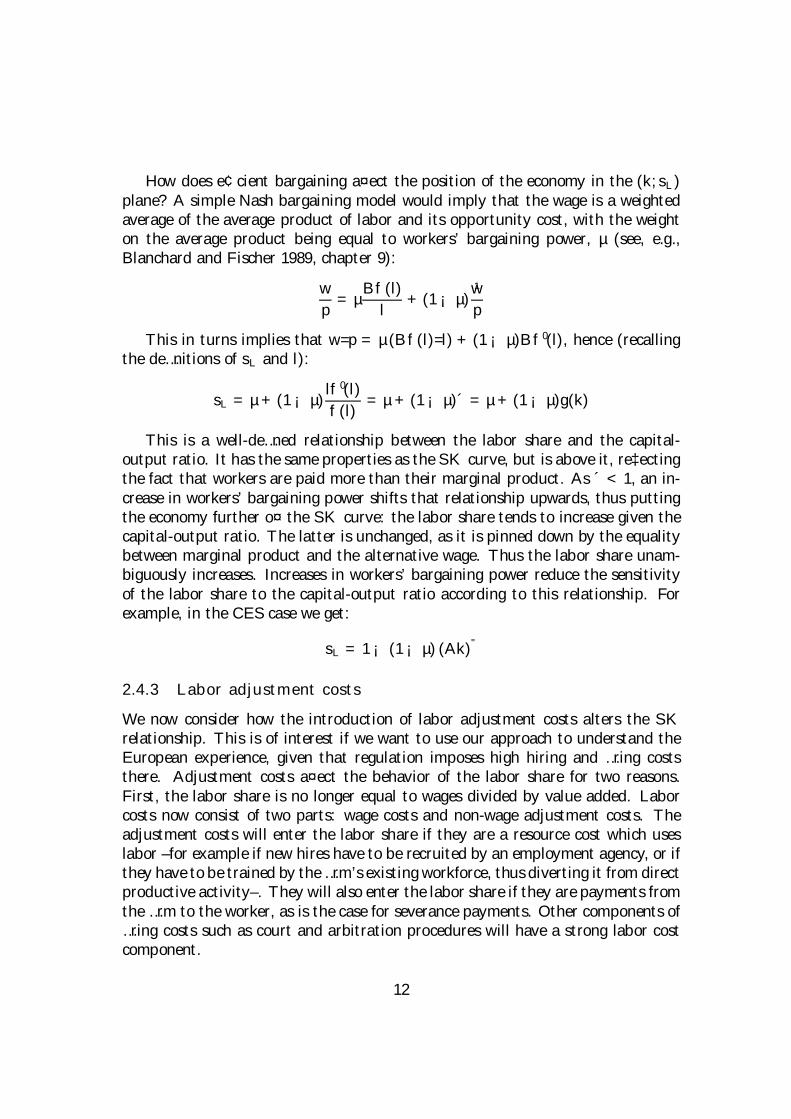
How does e¢cient bargaining a¤ect the position of the economy in the (k; sL)plane? A simple Nash bargaining model would imply that the wage is a weightedaverage of the average product of labor and its opportunity cost, with the weighton the average product being equal to workers’ bargaining power, µ (see, e.g.,Blanchard and Fischer 1989, chapter 9):

w

p= µ

Bf (l)

l+ (1¡ µ) ¹w

p

This in turns implies that w=p = µ (Bf(l)=l) + (1¡ µ)Bf 0(l), hence (recallingthe de…nitions of sL and l):

sL = µ + (1¡ µ) lf0(l)

f (l)= µ + (1¡ µ)´ = µ + (1¡ µ)g(k)

This is a well-de…ned relationship between the labor share and the capital-output ratio. It has the same properties as the SK curve, but is above it, re‡ectingthe fact that workers are paid more than their marginal product. As ´ < 1, an in-crease in workers’ bargaining power shifts that relationship upwards, thus puttingthe economy further o¤ the SK curve: the labor share tends to increase given thecapital-output ratio. The latter is unchanged, as it is pinned down by the equalitybetween marginal product and the alternative wage. Thus the labor share unam-biguously increases. Increases in workers’ bargaining power reduce the sensitivityof the labor share to the capital-output ratio according to this relationship. Forexample, in the CES case we get:

sL = 1¡ (1¡ µ) (Ak)"

2.4.3 Labor adjustment costs

We now consider how the introduction of labor adjustment costs alters the SKrelationship. This is of interest if we want to use our approach to understand theEuropean experience, given that regulation imposes high hiring and …ring coststhere. Adjustment costs a¤ect the behavior of the labor share for two reasons.First, the labor share is no longer equal to wages divided by value added. Laborcosts now consist of two parts: wage costs and non-wage adjustment costs. Theadjustment costs will enter the labor share if they are a resource cost which useslabor –for example if new hires have to be recruited by an employment agency, or ifthey have to be trained by the …rm’s existing workforce, thus diverting it from directproductive activity–. They will also enter the labor share if they are payments fromthe …rm to the worker, as is the case for severance payments. Other components of…ring costs such as court and arbitration procedures will have a strong labor costcomponent.

12

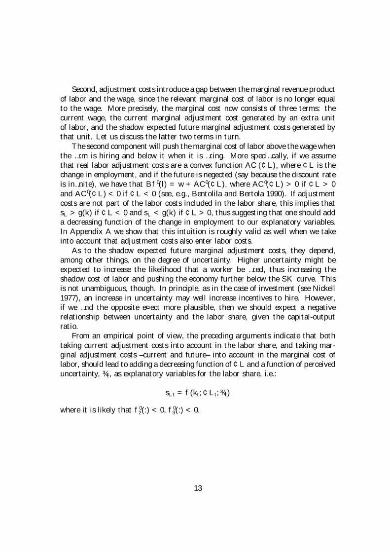
Second, adjustment costs introduce a gap between the marginal revenue productof labor and the wage, since the relevant marginal cost of labor is no longer equalto the wage. More precisely, the marginal cost now consists of three terms: thecurrent wage, the current marginal adjustment cost generated by an extra unitof labor, and the shadow expected future marginal adjustment costs generated bythat unit. Let us discuss the latter two terms in turn.

The second component will push the marginal cost of labor above the wage whenthe …rm is hiring and below it when it is …ring. More speci…cally, if we assumethat real labor adjustment costs are a convex function AC (¢L), where ¢L is thechange in employment, and if the future is negected (say because the discount rateis in…nite), we have that Bf 0(l) = w + AC 0(¢L), where AC 0(¢L) > 0 if ¢L > 0and AC 0(¢L) < 0 if ¢L < 0 (see, e.g., Bentolila and Bertola 1990). If adjustmentcosts are not part of the labor costs included in the labor share, this implies thatsL > g(k) if ¢L < 0 and sL < g(k) if ¢L > 0, thus suggesting that one should adda decreasing function of the change in employment to our explanatory variables.In Appendix A we show that this intuition is roughly valid as well when we takeinto account that adjustment costs also enter labor costs.

As to the shadow expected future marginal adjustment costs, they depend,among other things, on the degree of uncertainty. Higher uncertainty might beexpected to increase the likelihood that a worker be …red, thus increasing theshadow cost of labor and pushing the economy further below the SK curve. Thisis not unambiguous, though. In principle, as in the case of investment (see Nickell1977), an increase in uncertainty may well increase incentives to hire. However,if we …nd the opposite e¤ect more plausible, then we should expect a negativerelationship between uncertainty and the labor share, given the capital-outputratio.

From an empirical point of view, the preceding arguments indicate that bothtaking current adjustment costs into account in the labor share, and taking mar-ginal adjustment costs –current and future– into account in the marginal cost oflabor, should lead to adding a decreasing function of¢L and a function of perceiveduncertainty, ¾t, as explanatory variables for the labor share, i.e.:

sLt = f (kt;¢Lt; ¾t)

where it is likely that f 02(:) < 0, f03(:) < 0.

13

3 Evidence

We now investigate empirically the factors driving the evolution of the labor sharein 14 OECD countries since 1970, following our model. Data availability, however,precludes analyzing all the variables which are relevant according to the model.We focus on four sources of variation: movements along the SK relationship –i.e., shocks whose e¤ect on sL is entirely mediated by k, such as changes in theprices of capital and labor, and labor-augmenting technical progress–; one shifterof the SK curve, namely changes in the price of raw materials; and two sources ofmovements o¤ the SK schedule, namely changes in union bargaining power andlabor adjustment costs. We start by documenting a few stylized facts present in thedata, we then discuss the equation to be estimated and the econometric techniquesused, and we …nally show the empirical results.

3.1 Stylized facts

The SK schedule is a technological relationship, and so it is more appropriate toinvestigate it at the industry than at the country level. Therefore, we use indus-try data from the OECD International Sectoral Data Base (ISDB), which includesinformation on output, employment, capital, and factor shares for 14 OECD coun-tries over the period 1970-93, disaggregated at the 1- or 2-digit level. The set ofindustries analyzed does not span the whole economy, but comes close to doing so.Appendix B provides details on the database.

Our key variables are the labor share (sL) and the capital-output ratio (k). Thevariable sL is de…ned as the share of labor in nominal value added net of indirecttaxes and k is the ratio of the real capital stock to real value added. In other words,they correspond to esL and ek, as de…ned in the theory section, although we will omitthe e symbol for simplicity. Table 2 presents the overall statistics of these twovariables for all industries, countries, and years in the sample.7 Table 3 shows1973-93 averages (the sample period used in the econometric estimates, see below)for sL and k by industry and by country. For countries, averages for the wholeeconomies’ business sector are shown as well. The di¤erence between these and theISDB sample averages stem from the absence of a few sectors (sometimes only forcertain years), and from the inclusion of an imputation for the labor income of theself-employed in the former.8 Interestingly, within our sample, both variables varymore widely across industries than across countries: the range for the labor share,for example, goes from 20% in agriculture to 75% in machinery. These numbershelp us make the case for the industry approach to the data followed in this section.

7The remaining variables will be introduced below.8Descriptive statistics of the labor share in our sample when it is adjusted for the labor

remuneration of the self-employed appear in Table A2 of Appendix B.

14

3.2 Empirical speci…cation

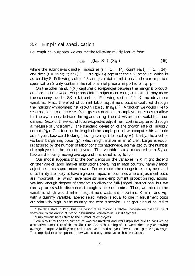
For empirical purposes, we assume the following multiplicative form:

sL;ijt = g(kijt; Sijt)h(Xijt) (15)

where the subindexes denote: industries (i = 1; :::; 14), countries (j = 1; :::; 14),and time (t = 1973; :::; 1993).9 Here g(k;S) captures the SK schedule, which isa¤ected by S. Following section 2.3, and given data limitations, under our empiricalspeci…cation S only contains the national real price of imported oil, qj=pj.

On the other hand, h(X) captures discrepancies between the marginal productof labor and the wage –wage bargaining, adjustment costs, etc.– which may movethe economy o¤ the SK relationship. Following section 2.4, X includes threevariables. First, the e¤ect of current labor adjustment costs is captured throughthe industry employment net growth rate (¢ lnnij).10 Although we would like toseparate out gross increases from gross reductions in employment, so as to allowfor the asymmetry between hiring and …ring, these ‡ows are not available in ourdataset. Second, the e¤ect of future expected adjustment costs is captured througha measure of uncertainty: the standard deviation of the growth rate of industryoutput (¾ij). Considering the length of the sample period, we compute this variableas a 5-year, backward-looking, moving average (denoted by »). Lastly, the e¤ect ofworkers’ bargaining power (µ), which might matter in an e¢cient bargains setup,is captured by the number of labor con‡icts nationwide, normalized by the numberof employees in the preceding year. This variable is also measured as a 5-yearbackward-looking moving average and it is denoted by flcrj .11

Our model suggests that the coe¢cients on the variables in X might dependon the type of labor market institutions prevailing in each country, namely laboradjustment costs and union power. For example, the change in employment anduncertainty are likely to have a greater impact in countries where adjustment costsare important, i.e., which have more stringent employment protection regulations.We lack enough degrees of freedom to allow for full-‡edged interactions, but wecan capture sizable di¤erences through simple dummies. Thus, we interact thevariables which would enter if adjustment costs are important, ¢ lnnij and e¾ij,with a dummy variable, labeled rigid, which is equal to one if adjustment costsare relatively high in the country and zero otherwise. The grouping of countries

9The data start in 1970, but the period of estimation is 1973-93 because we lose the …rst 3years due to the dating at t–2 of instrumental variables in …rst di¤erences.

10Employment here refers to the number of employees.11We also tried the the number of workers involved and work-days lost due to con‡icts as

alternative numerators of the con‡ict rate. As to the timing of lcr, were tried a 5-year movingaverage of output volatility centered around year t and a 3-year forward-looking moving average.The empirical results reported below were scarcely sensitive to these variations.

15

follows the information on severance pay and notice periods in Layard et al. (1991,p. 420). Australia, Canada, Denmark, Japan, the Netherlands, the UK, and theUS are classi…ed as having ‡exible labor markets, and the remaining countries ashaving rigid ones.

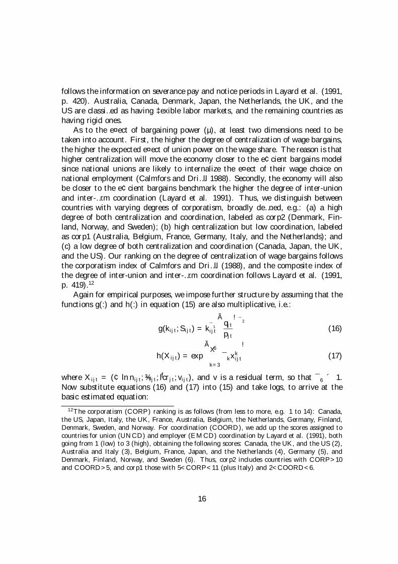
As to the e¤ect of bargaining power (µ), at least two dimensions need to betaken into account. First, the higher the degree of centralization of wage bargains,the higher the expected e¤ect of union power on the wage share. The reason is thathigher centralization will move the economy closer to the e¢cient bargains modelsince national unions are likely to internalize the e¤ect of their wage choice onnational employment (Calmfors and Dri…ll 1988). Secondly, the economy will alsobe closer to the e¢cient bargains benchmark the higher the degree of inter-unionand inter-…rm coordination (Layard et al. 1991). Thus, we distinguish betweencountries with varying degrees of corporatism, broadly de…ned, e.g.: (a) a highdegree of both centralization and coordination, labeled as corp2 (Denmark, Fin-land, Norway, and Sweden); (b) high centralization but low coordination, labeledas corp1 (Australia, Belgium, France, Germany, Italy, and the Netherlands); and(c) a low degree of both centralization and coordination (Canada, Japan, the UK,and the US). Our ranking on the degree of centralization of wage bargains followsthe corporatism index of Calmfors and Dri…ll (1988), and the composite index ofthe degree of inter-union and inter-…rm coordination follows Layard et al. (1991,p. 419).12

Again for empirical purposes, we impose further structure by assuming that thefunctions g(:) and h(:) in equation (15) are also multiplicative, i.e.:

g(kijt; Sijt) = k¯1ijt

Ãqjtpjt

!¯2(16)

h(Xijt) = exp

Ã6X

k=3

¯kxkijt

!(17)

where Xijt = (¢ ln nijt; ~¾ijt; flcrjt; vijt), and v is a residual term, so that ¯6 ´ 1.Now substitute equations (16) and (17) into (15) and take logs, to arrive at thebasic estimated equation:

12The corporatism (CORP ) ranking is as follows (from less to more, e.g. 1 to 14): Canada,the US, Japan, Italy, the UK, France, Australia, Belgium, the Netherlands, Germany, Finland,Denmark, Sweden, and Norway. For coordination (COORD), we add up the scores assigned tocountries for union (UNCD) and employer (EMCD) coordination by Layard et al. (1991), bothgoing from 1 (low) to 3 (high), obtaining the following scores: Canada, the UK, and the US (2),Australia and Italy (3), Belgium, France, Japan, and the Netherlands (4), Germany (5), andDenmark, Finland, Norway, and Sweden (6). Thus, corp2 includes countries with CORP>10and COORD>5, and corp1 those with 5<CORP<11 (plus Italy) and 2<COORD<6.

16

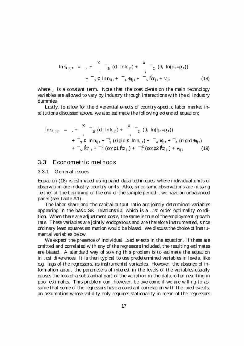
ln sL;ijt = ¸+X

i

¯1i (di ln kijt) +X

i

¯2i (di ln(qjt=pjt))

+ ¯3 ¢ lnnijt + ¯4 e¾ijt + ¯5flcrjt + vijt (18)

where ¸ is a constant term. Note that the coe¢cients on the main technologyvariables are allowed to vary by industry through interactions with the di industrydummies.

Lastly, to allow for the di¤erential e¤ects of country-speci…c labor market in-stitutions discussed above, we also estimate the following extended equation:

ln sL;ijt = ¸+X

i

¯1i (di ln kijt) +X

i

¯2i (di ln(qjt=pjt))

+ ¯3 ¢ lnnijt + ¯03 (rigid ¢ ln nijt) + ¯4 e¾ijt + ¯04 (rigid e¾ijt)

+ ¯5flcrjt + ¯ 05 (corp1 flcrjt) + ¯005 (corp2

flcrjt) + vijt (19)

3.3 Econometric methods

3.3.1 General issues

Equation (18) is estimated using panel data techniques, where individual units ofobservation are industry-country units. Also, since some observations are missing–either at the beginning or the end of the sample period–, we have an unbalancedpanel (see Table A1).

The labor share and the capital-output ratio are jointly determined variablesappearing in the basic SK relationship, which is a …rst order optimality condi-tion. When there are adjustment costs, the same is true of the employment growthrate. These variables are jointly endogenous and are therefore instrumented, sinceordinary least squares estimation would be biased. We discuss the choice of instru-mental variables below.

We expect the presence of individual …xed e¤ects in the equation. If these areomitted and correlated with any of the regressors included, the resulting estimatesare biased. A standard way of solving this problem is to estimate the equationin …rst di¤erences. It is then typical to use predetermined variables in levels, likee.g. lags of the regressors, as instrumental variables. However, the absence of in-formation about the parameters of interest in the levels of the variables usuallycauses the loss of a substantial part of the variation in the data, often resulting inpoor estimates. This problem can, however, be overcome if we are willing to as-sume that some of the regressors have a constant correlation with the …xed e¤ects,an assumption whose validity only requires stationarity in mean of the regressors

17

given the e¤ects, which moreover can be tested through the overidentifying restric-tions. Arellano and Bover (1995) note that, in this case, the …rst di¤erences ofthe predetermined variables are valid instruments for the equations in levels. Ine¤ect, they propose, in addition to using instruments in levels for the equations in…rst di¤erences, to use instruments in …rst di¤erences for the equations in levels.The model behind this …rst-di¤erences plus levels, or system, estimator is an in-termediate case between the …xed-e¤ects model, in which all explanatory variablesare potentially correlated with the e¤ects, and the random e¤ects model, in whichnone is. Arellano and Bover (1995) show that the system estimator may yield largee¢ciency gains vis-à-vis the pure …rst-di¤erence estimator (see also Blundell andBond, 1997).

We follow this proposal here. The estimation is carried out with the dynamicpanel data program DPD98, which implements the Arellano-Bover system estima-tor. This is an extension of the Generalized Method of Moments (GMM) procedureproposed by Arellano and Bond (1991), which exploits the appropriate orthogonal-ity conditions for the chosen instruments, minimizing the di¤erence between thesample moments and their zero population value.

3.3.2 Techniques

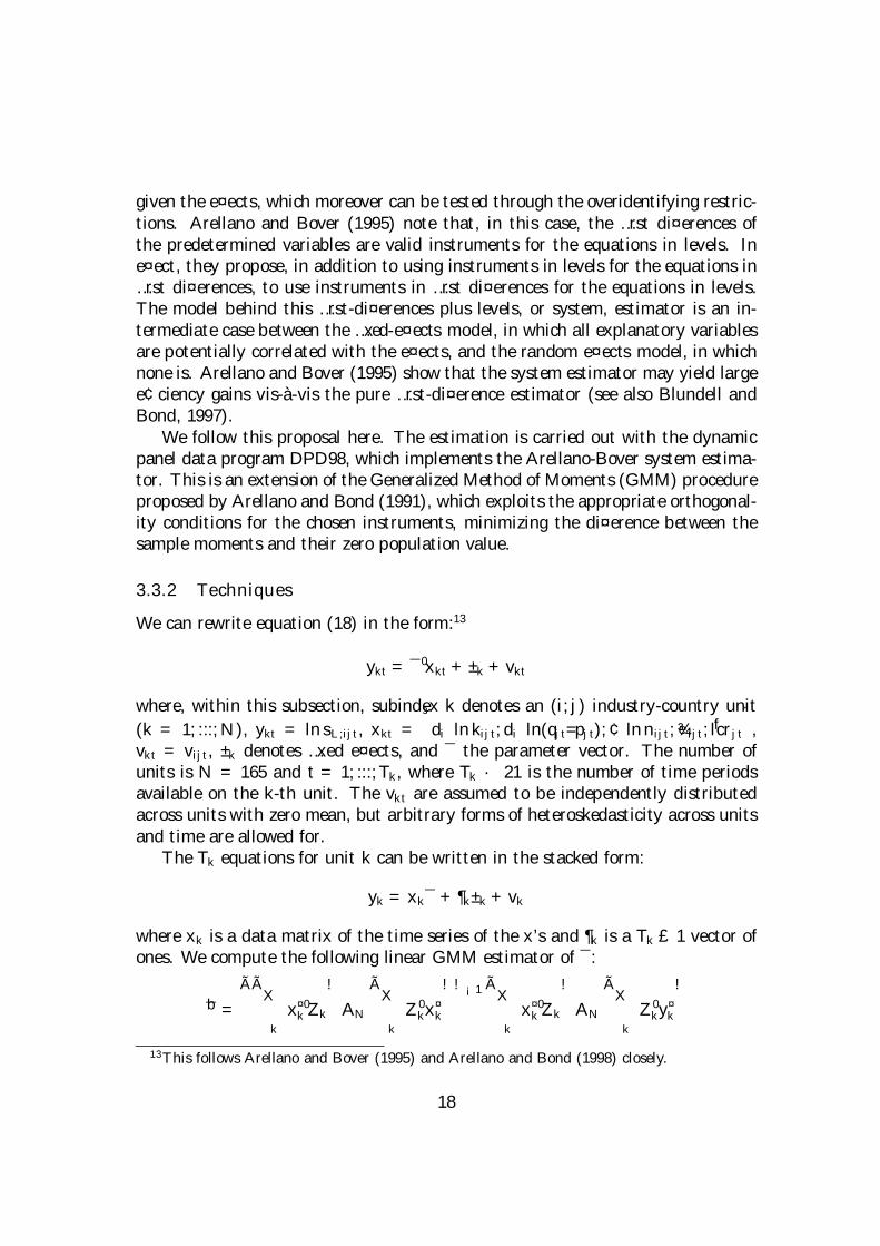
We can rewrite equation (18) in the form:13

ykt = ¯0xkt + ±k + vkt

where, within this subsection, subindex k denotes an (i; j) industry-country unit(k = 1; :::; N), ykt = ln sL;ijt, xkt =

³di ln kijt; di ln(qjt=pjt);¢ lnnijt; e¾ijt; flcrjt

´,

vkt = vijt, ±k denotes …xed e¤ects, and ¯ the parameter vector. The number ofunits is N = 165 and t = 1; :::; Tk, where Tk · 21 is the number of time periodsavailable on the k-th unit. The vkt are assumed to be independently distributedacross units with zero mean, but arbitrary forms of heteroskedasticity across unitsand time are allowed for.

The Tk equations for unit k can be written in the stacked form:

yk = xk¯ + ¶k±k + vk

where xk is a data matrix of the time series of the x’s and ¶k is a Tk £ 1 vector ofones. We compute the following linear GMM estimator of ¯:

b̄ =ÃÃX

k

x¤0k Zk

!AN

ÃX

k

Z 0kx¤k

!!¡1 ÃX

k

x¤0k Zk

!AN

ÃX

k

Z 0ky¤k

!

13This follows Arellano and Bover (1995) and Arellano and Bond (1998) closely.

18

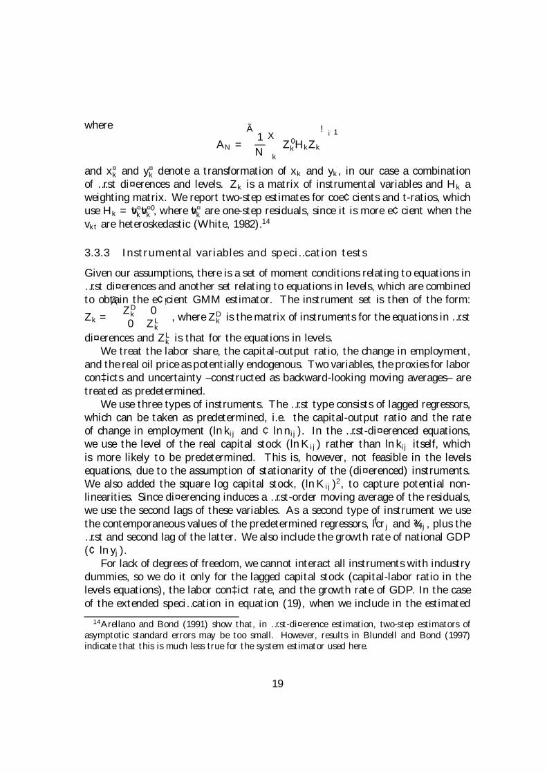
where

AN =

Ã1

N

X

k

Z 0kHkZk

!¡1

and x¤k and y¤k denote a transformation of xk and yk, in our case a combinationof …rst di¤erences and levels. Zk is a matrix of instrumental variables and Hk aweighting matrix. We report two-step estimates for coe¢cients and t-ratios, whichuse Hk = bv¤kbv¤0k , where bv¤k are one-step residuals, since it is more e¢cient when thevkt are heteroskedastic (White, 1982).14

3.3.3 Instrumental variables and speci…cation tests

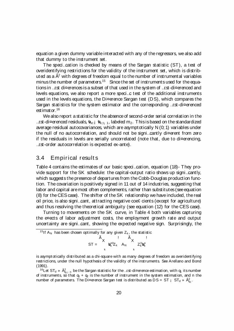
Given our assumptions, there is a set of moment conditions relating to equations in…rst di¤erences and another set relating to equations in levels, which are combinedto obtain the e¢cient GMM estimator. The instrument set is then of the form:

Zk =

ÃZDk 00 ZLk

!, where ZDk is the matrix of instruments for the equations in …rst

di¤erences and ZLk is that for the equations in levels.We treat the labor share, the capital-output ratio, the change in employment,

and the real oil price as potentially endogenous. Two variables, the proxies for laborcon‡icts and uncertainty –constructed as backward-looking moving averages– aretreated as predetermined.

We use three types of instruments. The …rst type consists of lagged regressors,which can be taken as predetermined, i.e. the capital-output ratio and the rateof change in employment (ln kij and ¢ lnnij). In the …rst-di¤erenced equations,we use the level of the real capital stock (lnKij) rather than ln kij itself, whichis more likely to be predetermined. This is, however, not feasible in the levelsequations, due to the assumption of stationarity of the (di¤erenced) instruments.We also added the square log capital stock, (lnKij)2, to capture potential non-linearities. Since di¤erencing induces a …rst-order moving average of the residuals,we use the second lags of these variables. As a second type of instrument we usethe contemporaneous values of the predetermined regressors, flcrj and e¾ij, plus the…rst and second lag of the latter. We also include the growth rate of national GDP(¢ ln yj).

For lack of degrees of freedom, we cannot interact all instruments with industrydummies, so we do it only for the lagged capital stock (capital-labor ratio in thelevels equations), the labor con‡ict rate, and the growth rate of GDP. In the caseof the extended speci…cation in equation (19), when we include in the estimated

14Arellano and Bond (1991) show that, in …rst-di¤erence estimation, two-step estimators ofasymptotic standard errors may be too small. However, results in Blundell and Bond (1997)indicate that this is much less true for the system estimator used here.

19

equation a given dummy variable interacted with any of the regressors, we also addthat dummy to the instrument set.

The speci…cation is checked by means of the Sargan statistic (ST ), a test ofoveridentifying restrictions for the validity of the instrument set, which is distrib-uted as a Â2 with degrees of freedom equal to the number of instrumental variablesminus the number of parameters.15 Since the set of instruments used for the equa-tions in …rst di¤erences is a subset of that used in the system of …rst-di¤erenced andlevels equations, we also report a more speci…c test of the additional instrumentsused in the levels equations, the Di¤erence Sargan test (DS), which compares theSargan statistics for the system estimator and the corresponding …rst-di¤erencedestimator.16

We also report a statistic for the absence of second-order serial correlation in the…rst-di¤erenced residuals, bvkt¡bvk;t¡1, labeledm2. This is based on the standardizedaverage residual autocovariances, which are asymptotically N (0; 1) variables underthe null of no autocorrelation, and should not be signi…cantly di¤erent from zeroif the residuals in levels are serially uncorrelated (note that, due to di¤erencing,…rst-order autocorrelation is expected ex-ante).

3.4 Empirical results

Table 4 contains the estimates of our basic speci…cation, equation (18)- They pro-vide support for the SK schedule: the capital-output ratio shows up signi…cantly,which suggests the presence of departures from the Cobb-Douglas production func-tion. The covariation is positively signed in 11 out of 14 industries, suggesting thatlabor and capital are most often complements, rather than substitutes (see equation(8) for the CES case). The shifter of the SK relationship we have included, the realoil price, is also signi…cant, attracting negative coe¢cients (except for agriculture)and thus resolving the theoretical ambiguity (see equation (12) for the CES case).

Turning to movements o¤ the SK curve, in Table 4 both variables capturingthe e¤ects of labor adjustment costs, the employment growth rate and outputuncertainty are signi…cant, showing the expected negative sign. Surprisingly, the

15If AN has been chosen optimally for any given Zk, the statistic

ST =

ÃX

k

bv¤0k Zk

!AN

ÃX

k

Z0kbv¤

k

!

is asymptotically distributed as a chi-square with as many degrees of freedom as overidentifyingrestrictions, under the null hypothesis of the validity of the instruments. See Arellano and Bond(1991).

16Let STd » Â2q1¡n be the Sargan statistic for the …rst-di¤erence estimation, with q1 its number

of instruments, so that q1 + q2 is the number of instrument in the system estimation, and n thenumber of parameters. The Di¤erence Sargan test is distributed as DS = ST ¡ STd » Â2

q2.

20

labor con‡ict rate, our proxy for workers’ bargaining power, attracts a negativecoe¢cient. One interpretation of this …nding relies on delayed responses to wagepushes (Caballero and Hammour 1998, see section 4 below).17 In any event, aswe shall see, the sign on this variable depends on the degree of corporatism in thecountry.

Test statistics for the validity of the instrument set and for second-order cor-relation in the residuals do not show any problems, although the Sargan test forthe validity of the extra instruments used in the system estimation, vis-à-vis thereduced set for the …rst-di¤erenced one, is passed at the margin.

Table 5 provides the estimation results for the extended speci…cation in equation(19). Di¤erent columns include a di¤erent set of regressors. In column (1) weinteract the employment growth rate with the labor market rigidity dummy andobtain that, as expected, it is signi…cant only in countries with more rigid labormarkets. Nevertheless, column (2) shows that output volatility, introduced so as tocapture the impact of future expected adjustment costs, does not appear to havea signi…cantly di¤erent e¤ect in countries with ‡exible and rigid labor markets.When we add the corporatism dummies interacted with the labor con‡ict rate, we…nd, in column (3), that the negative sign found in Table 4 comes from countrieswith relatively centralized bargaining but only a moderate amount of overall inter-union and inter-…rm coordination. The e¤ect is, on the other hand, positive forboth countries with decentralized bargaining and low coordination, and those withhighly centralized bargaining and high coordination. Regarding centralization, this…nding is reminiscent of the hump-shaped relationship between centralization andeconomic performance found by Calmfors and Dri¢ll (1988). As to coordination,in a cross-section analysis of 20 OECD countries, Nickell (1997), …nds that unioncoverage tends to raise unemployment, but this is o¤set if unions and employers cancoordinate their bargaining activities. The di¤erences we have uncovered regardingthe impact of labor con‡icts in coordinated vs. uncoordinated countries is a newinteresting …nding, relevant to this debate. At this stage of our research, we lack asimple explanation, but we believe this fact deserves further research.

In column (4) we can see that the results in columns (1) and (3) are robustto the joint introduction of the interactions added in those two columns. On theother hand, further addition of the interaction of output volatility with the rigiditydummy in column (5), while keeping all signs unchanged, lowers the signi…cance ofseveral coe¢cients.

We should note that our results may be a¤ected by measurement error. In our

17An alternative interpretation would require us to implicit model the cyclical behavior ofbargaining power. In Goodwin’s (1967) model of business cycles, unions tend to strike when thecapital share goes up. In his own words: ”The improved pro…tability carries the seed of its owndestruction by engendering a too vigorous expansion of output and employment, thus destroyingthe reserve army of labor and strengthening labor’s bargaining power” (p. 58).

21

data, sL is computed as the share of the remuneration of employees in value added.In general, part of the remuneration of the self-employed is a return to labor ratherthan to capital. However, there is no natural way of imputing that part. One wayof doing it is to assume that the self-employed earn the same wage as employees.However, typical calculations imply that the labor remuneration of self-employedlabor is actually lower than that of employees, which is not so surprising giventhat, for instance, social security taxes on the latter are generally much higherthan on the former. Thus, as a rough approximation, we have assumed that theself-employed earn two-thirds as much as employees (an assumption which givesestimates for the labor share which are close to those reported, for example, byEurostat in its European Economy review). Descriptive statistics of the samplewhen the adjusted labor share are given in Table A2 of Appendix C.

In Appendix C we present the estimation results for equation (18), using the ad-justed labor share, s¤L. Note that the sample size is now close to one-fourth smallerthan before, because average indirect tax rates, which are needed for computingthe adjusted labor share, are missing more often than the remaining variables. Thistends to render the econometric results less informative than those for the unad-justed labor share. Also, we do not expect to …nd exactly the same coe¢cients aswith the unadjusted labor share, since, for example, both …ring costs and unionpower a¤ect employees but not the self-employed. A comparison of the results inTables 4 and 5 with those of Tables A3 and A4 reveals a drop in the individualsigni…cance of the individual coe¢cients on the capital-output ratio and the realprice of oil. The signs of the coe¢cients on the shifters o¤ the SK schedule aremaintained, with the coe¢cients on the change in employment and output volatilitygenerally becoming stronger, and those on labor con‡icts becoming weaker.

In sum, we have tested our model of the determination of the labor share,albeit without imposing tight restrictions from the theory. The results con…rmthat a share-capital schedule exists, that the real price of oil shifts it, and thatthere are signi…cant deviations from it due to gaps between the marginal productof labor and the wage, arising from labor adjustment costs and union power. Wenow turn to a direct application of these empirical results.

4 Application: wage gaps revisited

4.1 Another look at the wage gap

Having checked that the theory is a reasonable guide to the behavior of the laborshare, we now employ it in trying to shed some light on the causes of Europeanunemployment, by revisiting the so-called wage gap (see Artus, 1984; Bruno andSachs, 1985). The wage gap approach typically takes the evolution of wages as

22

exogenous and compares them to the marginal product of labor at full employment.That is, recalling the production function Yt = F (Kt; BtLt), at time t the wagegap is de…ned as:

WGt =wt=pt

BtF 02(Kt; Bt ¹L)¡ 1 (20)

where ¹L is the full employment level. Then, assumptions are typically made aboutthe production function and the behavior of productivity in order to estimate apath for the denominator. This approach thus essentially amounts to looking atthe evolution of wages vis-à-vis labor productivity. This is quite close to lookingat the labor share, so that in most of continental Europe, where the labor sharehas risen and then fallen to its 1970 level (see Figure 4), it is generally concludedthat the wage gap has disappeared. The question is then how to reconcile this withthe persistence of high unemployment. In the wage gap literature, a low wage gapis generally interpreted as an indication that most unemployment is Keynesian,i.e. due to persistent slack associated with the failure of nominal prices and wagesto adjust. Given the persistence of high unemployment in Europe, we …nd thatinterpretation hard to believe.

How can our approach shed light on this issue? First, we can provide a newestimate of the wage gap, based on our analysis of the labor share, which maypotentially di¤er from those available in the literature. Second, we are able to de-compose changes in the wage gap in a new way. We have shown that we can breakdown movements in the labor share into three components: (i) movements alongthe SK schedule, which represent the optimal adjustment of …rm’s desired employ-ment to changes in prices and labor-augmenting technical progress; (ii) movementsof the SK schedule itself, which may arise from non-neutral technical progress, orequivalently changes in the price of imported materials; and (iii) movements o¤ theSK schedule, which represent discrepancies between the marginal product of la-bor and the wage. Possible sources of such discrepancies include adjustment costs,wage bargaining, and markups.

The …rst source of shocks –movements along the SK schedule– generates anegative relationship between the wage gap and employment: it simply capturesthe fact that, given the production function, the marginal product of labor isdecreasing with employment.

The second source of shocks –movements of the SK curve– will typically a¤ectthe marginal product of labor both at full and at current employment. It does notgenerate any clear correlation between employment and the wage gap. Both can goeither way, and this depends on how wages react to shocks. However, if the elasticityof the marginal product of labor with respect to employment is unchanged, thensuch shocks can only increase the wage gap if at the same time unemploymentincreases. In that case they will generate the same correlation between the two

23

variables as the …rst source of shocks.The last source of shocks –those putting the economy o¤ the SK curve, such as

an increase in uncertainty under labor adjustment costs– a¤ects the gap betweenthe marginal product of labor and the wage. An increase in that gap tends to reduceboth employment and wage, while increasing the marginal product. Thereforewe will observe an increase in unemployment associated with a fall in the wagegap. This source of shocks thus generates a negative correlation between these twovariables.

Analytically, this argument runs as follows.18 Let us rewrite equation (20)as 1 + WGt = wt=[ptBtF

02(Kt;Bt ¹Lt; St)]; where St captures shift factors in the

aggregate production function other than labor-augmenting technical progress.Then, the …rst-degree homogeneity of the production function and the de…nitionlt ´ BtLt=Kt, imply that:

1 +WGt = sLtYt

BtLtF 02(Kt; Bt ¹Lt; St)= sLt

f(lt; St)

ltf 01(¹lt; St)(21)

where ¹lt ´ Bt ¹Lt=Kt.Recall now the multiplicative form we assumed for the labor share in equation

(15): sLt = g(kt; St)h(Xt). Making use of the identity between g(k) and lf 0(l)=f(l)given by equation (3), equation (21) boils down to:

1 +WGt = h(Xt)f 01(lt; St)

f 01(¹lt; St)

This equation tells us that the wage gap is the product of the component ofthe labor share which is o¤ the SK schedule, times the ratio between the marginalproduct of labor at current employment and at full employment. This ratio isthe true wage gap; it tells us by how much wages would have to fall to eliminateunemployment, holding the production function and the Xt variables constant.The …rst term, on the other hand, captures a labor demand shift, which tells usthat, given the unemployment rate, wages must fall if the gap between the shadowcost of labor and the wage increases.

Note that our empirical estimates allow us to recover h(Xt), since we assumedin equation (17) that: h(Xt) = exp(§k¯kx

kt ), where Xt = (¢ lnnt; ~¾t; flcrt; vt).

Moreover, we can also approximate the second term, f 01(lt; St)=f01(¹lt; St), so as to

construct a series for the change in the wage gap and its components. We have:

¢WGt ¼ ¢ ln(1 +WGt)

¼ ¢ lnh(Xt) + ¢ln f01(lt; St)¡¢ ln f 01(¹lt; St)

18In this subsection we ignore the sector and country subindexes, as well as interactions withthe rigidity and corporatism dummies, for simplicity.

24

Noting that f 01(lt; St) = g(kt; St)=(ktlt) and denoting ¹kt = 1=f (¹lt; St) this can beexpressed as:

¢WGt ¼ ¢ lnh(Xt) +³¢ ln g(kt; St)¡¢ ln g(¹kt; St)

´

¡³¢ ln kt ¡¢ ln ¹kt

´¡

³¢ ln lt ¡¢ ln ¹lt

´

Now, using equations (3) and (4), and neglecting second order terms in u wehave that ln ¹kt ¼ ln kt¡ g(kt; St)ut and ¢ ln lt ¼ ¢ ln ¹lt¡¢ut: If we further assumethat g is isoelastic in k and log-separable in k and S; as in equation (16), g (kt; St) =k't °(St) = k

¯1t (qt=pt)

¯2, then the above equation can be rewritten as:

¢WGt ¼ ¢ lnh(Xt) + (' ¡ 1)¢ (k't °(St)ut) + ¢ut

or

¢WGt ¼ ¢ ln h(Xt) + (1¡ k't °(St)) ¢ut+('¡ 1)¢ (k't °(St)) ut + ' k't °(St) ¢ut (22)

or, for use in the next subsection:

¢WGt ¼ ¢ ln h(Xt) + (1¡ k't °(St)(1¡ ')) ¢ut + ('¡ 1)¢ (k't °(St)) ut (23)

The …rst term in equation (22) is the contribution of the labor demand shift. Ifit is equal to, say, -1%, it means that labor demand has fallen, so that wages mustfall by 1% to maintain unemployment constant. In other words, we are referring tolabor demand shocks which increase the wedge between the wage and the shadowcost of labor, thus the measured wage gap falls, since the wage is below the truelabor cost. We can further decompose this labor demand shift into an explainedcomponent (i.e., that explained by our explanatory variables, ¢n, e¾, and flcr) andan unexplained one, which is the contribution of the residual. This residual may beinterpreted as capturing changes in the price-cost markup, but it may also containother shocks.

The change in the true wage gap is the sum of all other terms in equation (22).If it is equal to, say, 1%, it means that wages would have to fall by 1% more in orderto restore full employment. This may be due to the fact that unemployment hasrisen or to a change in the shape of the marginal product schedule. It can be furtherdecomposed as follows. The second term, (1¡ k't °(St))¢ut, is the contribution tothe wage gap of changes in the discrepancy between the marginal product of laborat current employment and at full employment, holding the employment elasticityof output (i.e., g(k; S)) constant. The last, composite term, (' ¡ 1)¢(k't °(St))

25

ut + 'k't °(St) ¢ut, is the contribution of all changes in the employment elasticity

of output, whether induced by shifts in the production function captured by theshift factor S or by the variation of that elasticity as k and u change.

Note that while the true wage gap may fall at times of rising unemployment (ifthe employment elasticity of the marginal product falls), its value is always positiveif unemployment is positive. The reason is that if we start from zero unemployment,then the true wage gap must rise as ut rises, since (1¡ k't °(St)(1¡ ')) > 0.19 Inour empirical estimates, with the speci…cation of Table 4, this expression takes anaverage value of 0.35, being negative only for 60 observations (2% of the sample)in the agricultural sector.20

4.2 The evolution of wage gaps in two countries

We now show computed changes in the wage gaps for the US and (West) Germany,the only large economies for which there are data for all 14 industries over thefull period. In our computation we use the estimates in section 3, by consideringeach country as a basket of industries and applying the estimated coe¢cients tothe particular industry con…guration in the country. We use the parameter esti-mates obtained from the speci…cation in column (4) of Table 5, which allow thecoe¢cients on the variables in Xt to vary depending on the country’s degrees oflabor market rigidity and corporatism. The results would be very similar if wealternatively used the parameters in column (5). Along with data on unemploy-ment rates, those estimates then allow us to perform the decomposition in equation(23). Implementing it with industry level data entails some problems, discussed inAppendix A, which we solve by computing the aggregates in equation (23) as geo-metric averages, weighting industry-varying variables by their employment shares.

We should note from the outset that this procedure may only provide a roughapproximation to wage gaps, since parameter estimates from the panel result fromaveraging underlying coe¢cients which may vary across countries, and since, more-over, the list of sectors available for estimation is not exhaustive.

Figure 6 depicts the part of wage gap levels explained by the regressors in bothcountries, calculated by accumulating changes since 1973, taken as the referenceyear (=100). Figure 7 shows the decomposition described in equation (23) takingone term at a time (i.e. assuming changes in the other two terms were absent),also in index form. Figure 8 presents the contributions to the labor demand shiftsof each of the relevant variables: ¢ ln nt, ~¾t, and flcrt. Lastly, the computed shifts

19Note that (1 ¡ k't °(St)(1 ¡ ')) = 1 ¡ g(kt; St) + ktg

0(kt; St), kt = 1=f(lt), and g(kt; St) =ltf

0(lt)=f(lt). Thus, g0(kt; St) = ltf0(lt) ¡ (f 0(lt) + ltf

00(lt))(f(lt)=f0(lt)), so that ktg

0t(kt; St) =

g(kt; St) ¡ 1 ¡ ltf 00(lt)=f 0(lt). Consequently, 1 ¡ g(kt; St) + ktg0(kt; St) = ¡ltf 00(lt)=f 0(lt) > 0.20The same is true for the estimates in column (4) of Table 5, used in the next subsection.

26

and their components are provided in Table A5, which also contains the evolutionof wage gaps inclusive of the contribution of the unexplained residuals.

Figure 6 indicates increases in wage gaps in both Germany and the US in themid-1970s and early-1980s, but in Germany the increases are larger and tend todisappear more slowly. Moreover, Germany su¤ers a post-reuni…cation surge in thewage gap which is absent in the US.

Figure 7 suggests that the marginal product of labor in Germany is around 2%higher, holding capital constant, than what it would be if unemployment was at its1973 level. The equivalent …gure for the US, where unemployment has also risen butby less, is below one percent. The …gure also reveals that in both countries there arelarge shifts in labor demand that a¤ect the measured wage gap. In Germany thesemovements are countercyclical and Figure 8 shows that they are chie‡y explainedby the contribution of adjustment costs: in recessions the shadow cost of labor goesdown relative to the wage, labor demand is thus high –meaning higher than absentadjustment costs– and so is the measured wage gap, as in recessions adjustmentcosts drive a positive wedge between the wage and the marginal product of labor.Other components, such as changes in union power or uncertainty, play virtually norole in Germany. In the United States, the labor demand component is more erraticand less persistent. It is also chie‡y driven by adjustment costs, but a continuingdecline in union power has also contributed to bringing down wages relative to themarginal product of labor. Contrary to the conventional wisdom, there is virtuallyno contribution to the wage gap, in either country, by factors that change theshape of the production function, e.g. changes in the capital-output ratio –drivenby labor-augmenting technical progress or movements in factor costs such as wagesand interest rates– or in the real price of oil.

Recently Blanchard (1997,1998) and Caballero and Hammour (1998) have soughtto explain the di¤erent evolution of unemployment in continental European andAnglo-Saxon countries since the 1970s, bearing in mind the evolution of the laborshare. Blanchard (1997) explains such evolution, in continental Europe, as result-ing from responses to labor supply shifts in the 1970s (oil shocks, the productivitygrowth slowdown, changes in labor institutions) and labor demand shocks in the1980s. His attempt at distinguishing between shifts in the distribution of rents andbiased technological change as sources of the latter is however inconclusive. Ourresults support the idea that the European unemployment experience cannot beunderstood without recourse to signi…cant labor demand shifts. While they arenot readily comparable to his, since we follow a di¤erent approach, there are somesimilarities. First, Blanchard (1997) computes much higher labor demand shiftsfor Germany than for the US (Germany: –6% over 1970-81, 3% over 1981-95; US:–3% and 0%, respectively), in accordance with our own estimates. Second, Blan-chard (1998) reports computations of yearly labor demand shifts only for France,which moreover vary depending on two exogenously chosen parameters: the degree

27

of wage inertia and the elasticity of substitution of a CES production function.Nevertheless, a common theme is that computed labor demand shifts for Francetend to be negative in the mid-1970s, positive in the …rst half of the 1980s, andnegative again in the second half of the 1980s, while our results for Germany followa similar pattern (cfr. his Figure 11 with our Table A4).21

As the …gures in Table A4 make clear, however, the evolutions commented sofar are dwarfed by the contribution of the residual, i.e. the unexplained componentin the gap between wages and marginal product. In the case of Germany, thisunexplained component accounts for most of the hump-shaped pattern of the laborshare in the 1970s and 1980s. This result casts doubts over the interpretation ofthat stylized fact suggested by Caballero and Hammour (1998). According to theseauthors, the hump shape is due to the lagged response of capital-labor substitutionto initial wage pushes. That is, wage pushes increase the labor share in the shortrun because of sluggishness in labor demand adjustment (due to institutions whichraise labor’s capability of appropriating rents, such as …ring costs, unemploymentbene…ts, and social security contributions; and to increases in speci…city). Thesepushes, however, reduce the labor share in the long run, as substitution of capitalfor labor works its way. Such pattern is consistent with a negatively sloped SKcurve, and the e¤ect of adjustment costs that we have found. But the contributionsof ¢n and k actually fail to pick up the hump-shaped pattern for the labor share,which is mostly driven by the residual. This suggests that we have to look for otherexplanations.

An interesting …nding is that the residual in the US exhibits the same hump-shaped pattern as in Germany, despite the fact that the total labor share doesnot exhibit this behavior. Thus it seems that our empirical procedure allows usto recover some labor demand shock common to the two countries, which was notapparent in the raw data. At this stage, we can only speculate about the natureof that demand shock. The obvious interpretation in terms of markups seemsimplausible; only further research can uncover the factors underlying this similarevolution of the residuals in Germany and the US.

5 Conclusions

In this paper we show that movements in the labor share can be fruitfully de-composed into movements along a technology-determined curve –the share-capital(SK) schedule–, shifts of this locus, and deviations from it. Movements along theSK curve capture changes in factor prices such as wage pushes and changes in realinterest rates, as well as the contribution of labor-augmenting technical progress.

21For Germany, Blanchard (1997) simply reports a labor demand shift of -6% over 1970-81 andof 3% over 1981-95.

28

The curve is itself shifted by factors such as non-labor embodied technical progressor changes in the price of imported materials. Lastly, other sources of variation ofthe labor share are represented by movements o¤ the SK curve, and are accountedfor by deviations from marginal cost pricing such as changes in markups, laboradjustment costs, and changes in workers’ bargaining power.

We analyze the performance of the model empirically, using data on a panelof 14 industries in 14 OECD countries, over the period 1973-93, by estimatingthe relationship between the labor share and the capital-output ratio, controllingfor variables intended to capture some of the factors mentioned above. In theestimation we follow a recent proposal by Arellano and Bover (1995) of a systemestimator for panel data, i.e. a generalized method of moments estimator withinstrumental variables which exploits the information contained in the relationshipbetween the variables in both levels and …rst di¤erences.

We …nd a signi…cant relationship between the two key variables, i.e. favorableevidence for the SK schedule. There is also evidence of movements in the laborshare due to either shifts of the SK schedule, arising from changes in the real priceof oil, and of movements o¤ such schedule, arising from labor adjustment costs andchanges in workers’ bargaining power.

We then employ the empirical estimates in trying to shed light on the sourcesof European unemployment, through the concept of wage gaps, i.e. the di¤erencebetween wages and the marginal product of labor. We compute wage gaps in twolarge economies, the US and Germany and decompose its evolution according tothe theoretical model. Our results indicate that there are sizable labor demandshifts in both countries, especially in Germany, where they essentially arise fromthe presence of labor adjustment costs.

29

Appendix AAlgebraic derivations

A.1 Relationship between the labor share and the skill premium (section2.3.2)

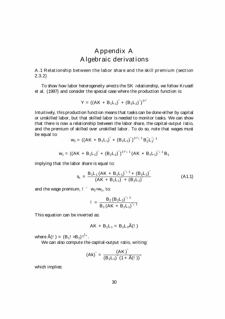
To show how labor heterogeneity a¤ects the SK relationship, we follow Krusellet al. (1997) and consider the special case where the production function is:

Y = ((AK +B1L1)" + (B2L2)

")1="

Intuitively, this production function means that tasks can be done either by capitalor unskilled labor, but that skilled labor is needed to monitor tasks. We can showthat there is now a relationship between the labor share, the capital-output ratio,and the premium of skilled over unskilled labor. To do so, note that wages mustbe equal to:

w2 = ((AK +B1L1)" + (B2L2)

")1="¡1

B"2L"¡12

w1 = ((AK +B1L1)" + (B2L2)

")1="¡1 (AK +B1L1)"¡1B1

implying that the labor share is equal to:

sL =B1L1 (AK +B1L1)

"¡1 + (B2L2)"

(AK +B1L1)" + (B2L2)

" (A1.1)

and the wage premium, ! ´ w2=w1, to:

! =B2 (B2L2)

"¡1

B1 (AK +B1L1)"¡1

This equation can be inverted as:

AK +B1L1 = B2L2Ã(!)

where Ã(!) = (B1!=B2)1

1¡" .We can also compute the capital-output ratio, writing:

(Ak)" =(AK)"

(B2L2)" (1 + Ã(!))"

which implies:

30

AK = AkB2L2 (1 + Ã(!)")1="

Substituting this equation into the previous one, we may express B1L1 as afunction of B2L2 and !, which we may then substitute, alongside with the lattertwo equations, into equation (A1.1) to get:

sL = 1¡ AkÃ(!)"¡1 (1 + Ã(!)")1="¡1

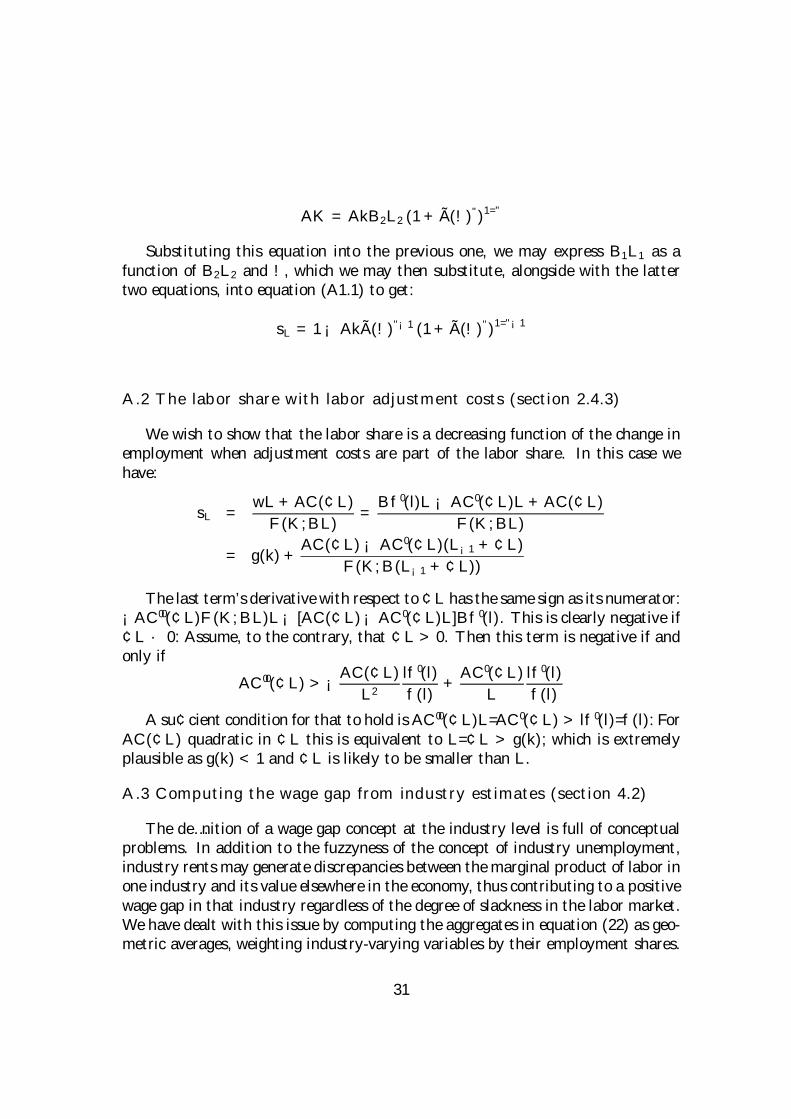
A.2 The labor share with labor adjustment costs (section 2.4.3)

We wish to show that the labor share is a decreasing function of the change inemployment when adjustment costs are part of the labor share. In this case wehave:

sL =wL+AC(¢L)

F (K;BL)=Bf 0(l)L ¡AC 0(¢L)L+AC(¢L)

F (K;BL)

= g(k) +AC(¢L)¡ AC 0(¢L)(L¡1 +¢L)

F (K;B(L¡1 +¢L))

The last term’s derivative with respect to¢L has the same sign as its numerator:¡AC 00(¢L)F (K;BL)L¡ [AC(¢L)¡AC 0(¢L)L]Bf 0(l). This is clearly negative if¢L · 0: Assume, to the contrary, that ¢L > 0. Then this term is negative if andonly if

AC 00(¢L) > ¡AC(¢L)L2

lf 0(l)

f (l)+AC 0(¢L)

L

lf 0(l)

f(l)

A su¢cient condition for that to hold is AC 00(¢L)L=AC 0(¢L) > lf 0(l)=f (l): ForAC(¢L) quadratic in ¢L this is equivalent to L=¢L > g(k); which is extremelyplausible as g(k) < 1 and ¢L is likely to be smaller than L.

A.3 Computing the wage gap from industry estimates (section 4.2)

The de…nition of a wage gap concept at the industry level is full of conceptualproblems. In addition to the fuzzyness of the concept of industry unemployment,industry rents may generate discrepancies between the marginal product of labor inone industry and its value elsewhere in the economy, thus contributing to a positivewage gap in that industry regardless of the degree of slackness in the labor market.We have dealt with this issue by computing the aggregates in equation (22) as geo-metric averages, weighting industry-varying variables by their employment shares.

31

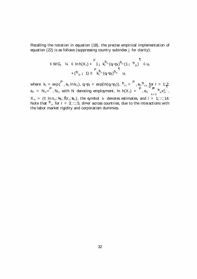
Recalling the notation in equation (18), the precise empirical implementation ofequation (22) is as follows (suppressing country subindex j for clarity):

¢WGt ¼ ¢ ln h(Xt) +µ1¡ kb̄1tt (qt=pt)

b̄2t(1¡ b̄

1t)¶¢ut

+(b̄1t ¡ 1) ¢µkb̄1tt (qt=pt)

b̄2t

¶ut

where: kt = exp (Pi eit ln kit), qt=pt = exp(ln(qt=pt)), b̄

rt =Pi eit

b̄rit for r = 1; 2,

eit = Nit=PiNit with N denoting employment, ln h(Xt) =

Pi eit

µ6Pk=3

b̄kxkit

¶,

Xit = (¢ ln nit; ~¾it; flcrt; bvit), the symbol b denotes estimates, and i = 1; :::; 14.Note that b̄

rt for r = 3; :::; 5, di¤er across countries, due to the interactions withthe labor market rigidity and corporatism dummies.

32

Appendix BData sources and de…nitions of variables

The variables we use in the econometric estimation are constructed from the OECDInternational Sectoral Data Base (ISDB) 1996, documented in OECD (1996). Itcovers the period 1960-95, but disaggregated data on a su¢cient scale for mostvariables are available for 1970-93. The variables we use are as follows (originalISDB variables denoted by their own acronyms in capital letters):

Labor share: sL = 1¡OP:Capital-output ratio: k = KTVD=GDPD:Real oil price: q=p= Nominal oil price/GDP de‡ator=(PO£ER)=(GDP=GDPV ):Labor con‡ict rate: lcr = Number of labor con‡icts (strikes+lock-outs) /Numberof employees in the preceding year (Source: CEP-OECD Data Set, documented inBell and Dryden 1996).Adjusted labor share: s¤L = WSSS (ET=EE)=(GDP (1¡ IND))

where:² OP = Ratio of gross operating surplus to value added minus net indirect taxes.² KTV D = Gross capital stock, at 1990 prices and 1990 PPPs (US dollars).² GDPD = Value added at market prices, at 1990 prices and 1990 PPPs. (USdollars).² PO = Price of oil in dollars (Source: International Monetary Fund, InternationalFinancial Statistics, IFS).² ER = Exchange rate vis-à-vis the dollar (Market rate/Par or Central rate, periodaverage. Source: IFS).² GDP = Value added at market prices, current prices, national currency.² GDPV = Value added at market prices, at 1990 prices, national currency.² WSSS = Compensation of employees, at current prices, national currency.² EE = Number of employees.² ET = Total employment.² IND = Ratio of net indirect taxes to value added.

The sectoral breakdown used distinguishes between 14 industries. The num-ber of observations available for the econometric estimation by country, year, andindustry are in Table A1.

33

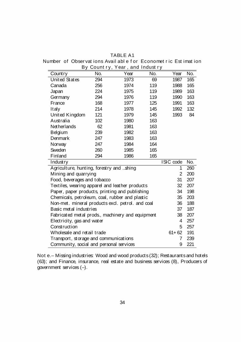
TABLE A1Number of Observations Available for Econometric Estimation

By Country, Year, and IndustryCountry No. Year No. Year No.United States 294 1973 69 1987 165Canada 256 1974 119 1988 165Japan 224 1975 119 1989 163Germany 294 1976 119 1990 163France 168 1977 125 1991 163Italy 214 1978 145 1992 132United Kingdom 121 1979 145 1993 84Australia 102 1980 163Netherlands 62 1981 163Belgium 239 1982 163Denmark 247 1983 163Norway 247 1984 164Sweden 260 1985 165Finland 294 1986 165Industry ISIC code No.Agriculture, hunting, forestry and …shing 1 260Mining and quarrying 2 200Food, beverages and tobacco 31 207Textiles, wearing apparel and leather products 32 207Paper, paper products, printing and publishing 34 198Chemicals, petroleum, coal, rubber and plastic 35 203Non-met. mineral products excl. petrol. and coal 36 188Basic metal industries 37 187Fabricated metal prods., machinery and equipment 38 207Electricity, gas and water 4 257Construction 5 257Wholesale and retail trade 61+62 191Transport, storage and communications 7 239Community, social and personal services 9 221

Note.– Missing industries: Wood and wood products (32); Restaurants and hotels(63); and Finance, insurance, real estate and business services (8), Producers ofgovernment services (–).

34

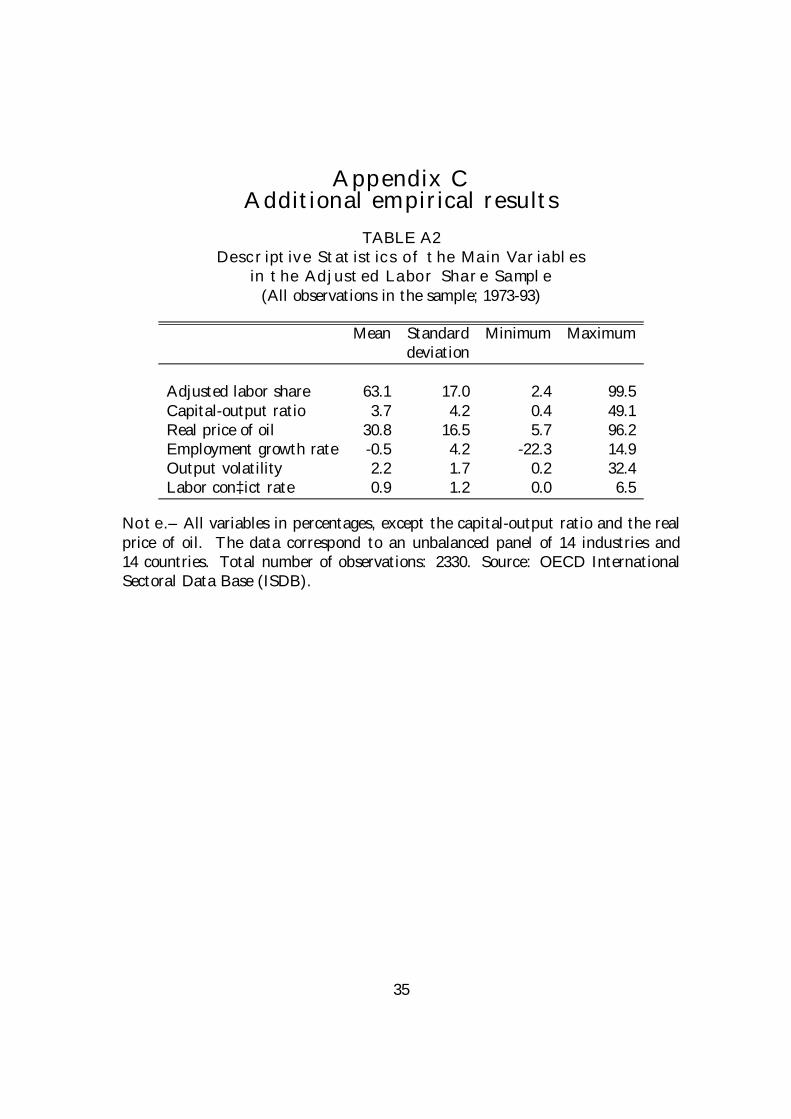
Appendix CAdditional empirical results

TABLE A2Descriptive Statistics of the Main Variables

in the Adjusted Labor Share Sample(All observations in the sample; 1973-93)

Mean Standard Minimum Maximumdeviation

Adjusted labor share 63.1 17.0 2.4 99.5Capital-output ratio 3.7 4.2 0.4 49.1Real price of oil 30.8 16.5 5.7 96.2Employment growth rate -0.5 4.2 -22.3 14.9Output volatility 2.2 1.7 0.2 32.4Labor con‡ict rate 0.9 1.2 0.0 6.5

Note.– All variables in percentages, except the capital-output ratio and the realprice of oil. The data correspond to an unbalanced panel of 14 industries and14 countries. Total number of observations: 2330. Source: OECD InternationalSectoral Data Base (ISDB).

35

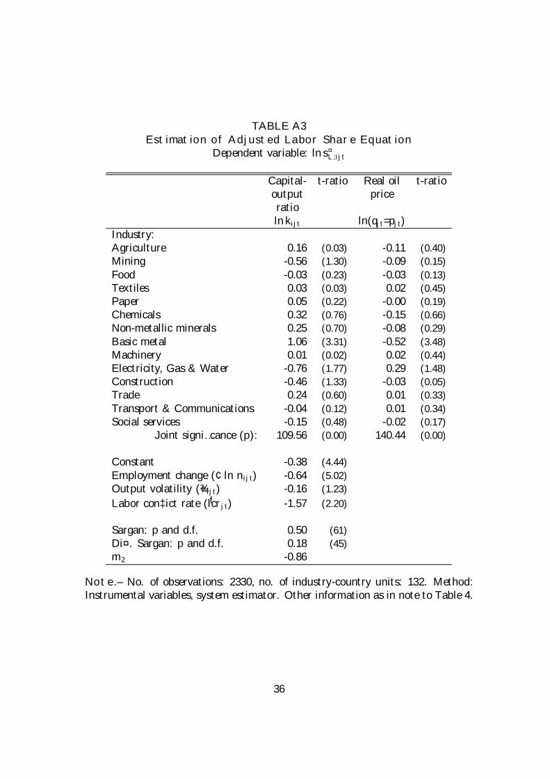
TABLE A3Estimation of Adjusted Labor Share Equation

Dependent variable: ln s¤L;ijt

Capital- t-ratio Real oil t-ratiooutput priceratioln kijt ln(qjt=pjt)

Industry:Agriculture 0.16 (0.03) -0.11 (0.40)Mining -0.56 (1.30) -0.09 (0.15)Food -0.03 (0.23) -0.03 (0.13)Textiles 0.03 (0.03) 0.02 (0.45)Paper 0.05 (0.22) -0.00 (0.19)Chemicals 0.32 (0.76) -0.15 (0.66)Non-metallic minerals 0.25 (0.70) -0.08 (0.29)Basic metal 1.06 (3.31) -0.52 (3.48)Machinery 0.01 (0.02) 0.02 (0.44)Electricity, Gas & Water -0.76 (1.77) 0.29 (1.48)Construction -0.46 (1.33) -0.03 (0.05)Trade 0.24 (0.60) 0.01 (0.33)Transport & Communications -0.04 (0.12) 0.01 (0.34)Social services -0.15 (0.48) -0.02 (0.17)

Joint signi…cance (p): 109.56 (0.00) 140.44 (0.00)

Constant -0.38 (4.44)Employment change (¢ln nijt) -0.64 (5.02)Output volatility (e¾ijt) -0.16 (1.23)Labor con‡ict rate ( flcrjt) -1.57 (2.20)

Sargan: p and d.f. 0.50 (61)Di¤. Sargan: p and d.f. 0.18 (45)m2 -0.86

Note.– No. of observations: 2330, no. of industry-country units: 132. Method:Instrumental variables, system estimator. Other information as in note to Table 4.

36

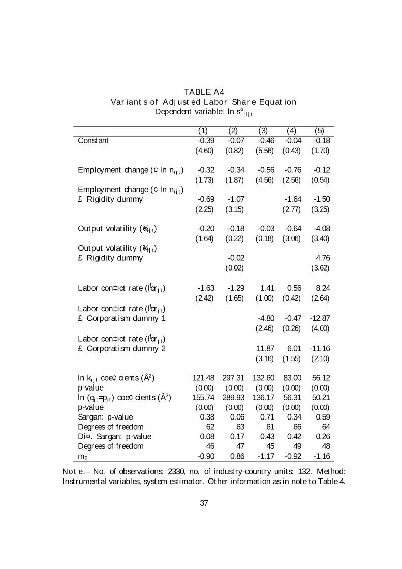
TABLE A4Variants of Adjusted Labor Share Equation

Dependent variable: ln s¤L;ijt

(1) (2) (3) (4) (5)Constant -0.39 -0.07 -0.46 -0.04 -0.18

(4.60) (0.82) (5.56) (0.43) (1.70)

Employment change (¢ln nijt) -0.32 -0.34 -0.56 -0.76 -0.12(1.73) (1.87) (4.56) (2.56) (0.54)

Employment change (¢ln nijt)£ Rigidity dummy -0.69 -1.07 -1.64 -1.50

(2.25) (3.15) (2.77) (3.25)

Output volatility (e¾ijt) -0.20 -0.18 -0.03 -0.64 -4.08(1.64) (0.22) (0.18) (3.06) (3.40)

Output volatility (e¾ijt)£ Rigidity dummy -0.02 4.76

(0.02) (3.62)

Labor con‡ict rate ( flcrjt) -1.63 -1.29 1.41 0.56 8.24(2.42) (1.65) (1.00) (0.42) (2.64)

Labor con‡ict rate ( flcrjt)£ Corporatism dummy 1 -4.80 -0.47 -12.87

(2.46) (0.26) (4.00)Labor con‡ict rate ( flcrjt)£ Corporatism dummy 2 11.87 6.01 -11.16

(3.16) (1.55) (2.10)

ln kijt coe¢cients (Â2) 121.48 297.31 132.60 83.00 56.12p-value (0.00) (0.00) (0.00) (0.00) (0.00)ln (qjt=pjt) coe¢cients (Â2) 155.74 289.93 136.17 56.31 50.21p-value (0.00) (0.00) (0.00) (0.00) (0.00)Sargan: p-value 0.38 0.06 0.71 0.34 0.59Degrees of freedom 62 63 61 66 64Di¤. Sargan: p-value 0.08 0.17 0.43 0.42 0.26Degrees of freedom 46 47 45 49 48m2 -0.90 0.86 -1.17 -0.92 -1.16

Note.– No. of observations: 2330, no. of industry-country units: 132. Method:Instrumental variables, system estimator. Other information as in note to Table 4.

37

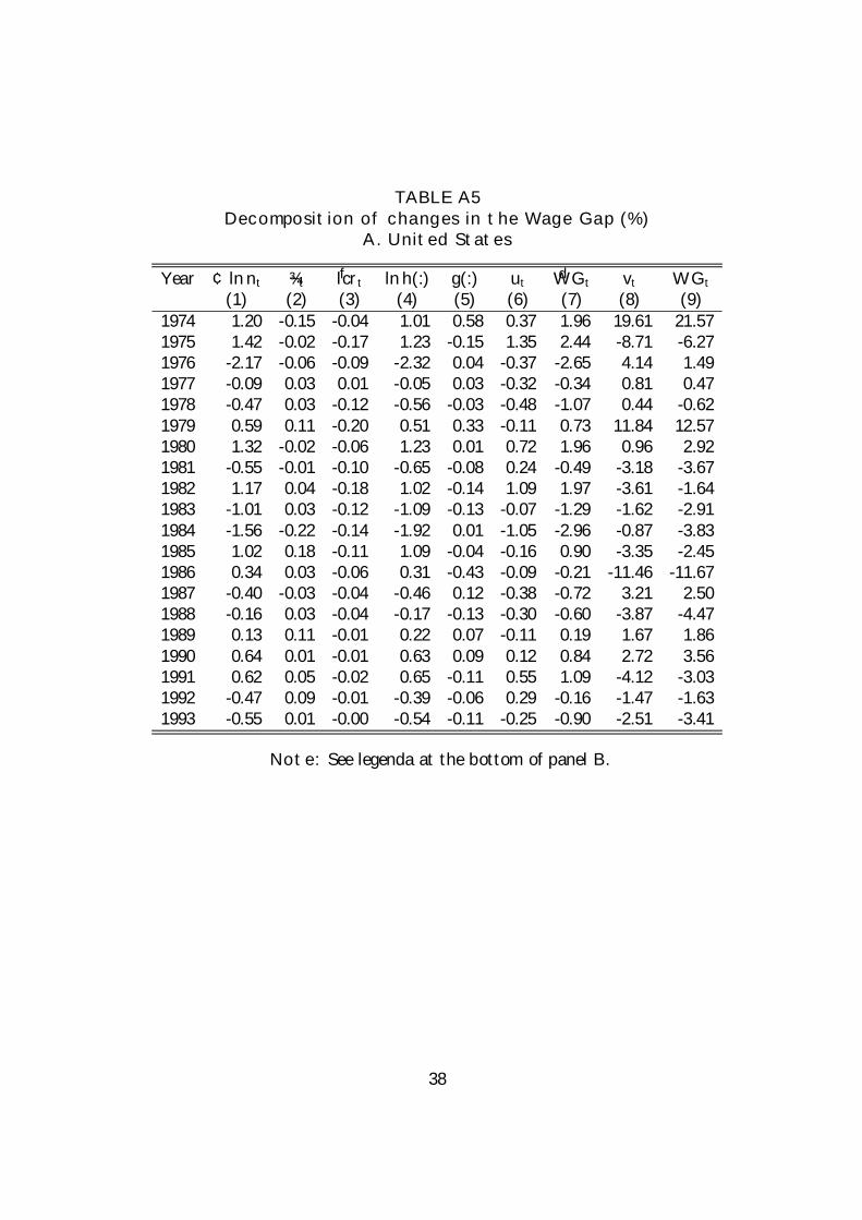
TABLE A5Decomposition of changes in the Wage Gap (%)

A. United States

Year ¢ ln nt ~¾t flcrt ln h(:) g(:) ut dWGt vt WGt(1) (2) (3) (4) (5) (6) (7) (8) (9)

1974 1.20 -0.15 -0.04 1.01 0.58 0.37 1.96 19.61 21.571975 1.42 -0.02 -0.17 1.23 -0.15 1.35 2.44 -8.71 -6.271976 -2.17 -0.06 -0.09 -2.32 0.04 -0.37 -2.65 4.14 1.491977 -0.09 0.03 0.01 -0.05 0.03 -0.32 -0.34 0.81 0.471978 -0.47 0.03 -0.12 -0.56 -0.03 -0.48 -1.07 0.44 -0.621979 0.59 0.11 -0.20 0.51 0.33 -0.11 0.73 11.84 12.571980 1.32 -0.02 -0.06 1.23 0.01 0.72 1.96 0.96 2.921981 -0.55 -0.01 -0.10 -0.65 -0.08 0.24 -0.49 -3.18 -3.671982 1.17 0.04 -0.18 1.02 -0.14 1.09 1.97 -3.61 -1.641983 -1.01 0.03 -0.12 -1.09 -0.13 -0.07 -1.29 -1.62 -2.911984 -1.56 -0.22 -0.14 -1.92 0.01 -1.05 -2.96 -0.87 -3.831985 1.02 0.18 -0.11 1.09 -0.04 -0.16 0.90 -3.35 -2.451986 0.34 0.03 -0.06 0.31 -0.43 -0.09 -0.21 -11.46 -11.671987 -0.40 -0.03 -0.04 -0.46 0.12 -0.38 -0.72 3.21 2.501988 -0.16 0.03 -0.04 -0.17 -0.13 -0.30 -0.60 -3.87 -4.471989 0.13 0.11 -0.01 0.22 0.07 -0.11 0.19 1.67 1.861990 0.64 0.01 -0.01 0.63 0.09 0.12 0.84 2.72 3.561991 0.62 0.05 -0.02 0.65 -0.11 0.55 1.09 -4.12 -3.031992 -0.47 0.09 -0.01 -0.39 -0.06 0.29 -0.16 -1.47 -1.631993 -0.55 0.01 -0.00 -0.54 -0.11 -0.25 -0.90 -2.51 -3.41

Note: See legenda at the bottom of panel B.

38

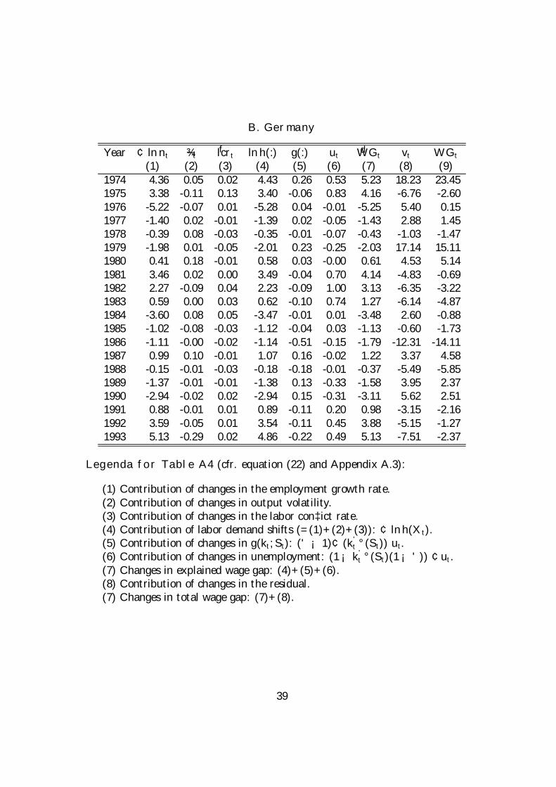
B. Germany

Year ¢ ln nt ~¾t flcrt ln h(:) g(:) ut dWGt vt WGt(1) (2) (3) (4) (5) (6) (7) (8) (9)

1974 4.36 0.05 0.02 4.43 0.26 0.53 5.23 18.23 23.451975 3.38 -0.11 0.13 3.40 -0.06 0.83 4.16 -6.76 -2.601976 -5.22 -0.07 0.01 -5.28 0.04 -0.01 -5.25 5.40 0.151977 -1.40 0.02 -0.01 -1.39 0.02 -0.05 -1.43 2.88 1.451978 -0.39 0.08 -0.03 -0.35 -0.01 -0.07 -0.43 -1.03 -1.471979 -1.98 0.01 -0.05 -2.01 0.23 -0.25 -2.03 17.14 15.111980 0.41 0.18 -0.01 0.58 0.03 -0.00 0.61 4.53 5.141981 3.46 0.02 0.00 3.49 -0.04 0.70 4.14 -4.83 -0.691982 2.27 -0.09 0.04 2.23 -0.09 1.00 3.13 -6.35 -3.221983 0.59 0.00 0.03 0.62 -0.10 0.74 1.27 -6.14 -4.871984 -3.60 0.08 0.05 -3.47 -0.01 0.01 -3.48 2.60 -0.881985 -1.02 -0.08 -0.03 -1.12 -0.04 0.03 -1.13 -0.60 -1.731986 -1.11 -0.00 -0.02 -1.14 -0.51 -0.15 -1.79 -12.31 -14.111987 0.99 0.10 -0.01 1.07 0.16 -0.02 1.22 3.37 4.581988 -0.15 -0.01 -0.03 -0.18 -0.18 -0.01 -0.37 -5.49 -5.851989 -1.37 -0.01 -0.01 -1.38 0.13 -0.33 -1.58 3.95 2.371990 -2.94 -0.02 0.02 -2.94 0.15 -0.31 -3.11 5.62 2.511991 0.88 -0.01 0.01 0.89 -0.11 0.20 0.98 -3.15 -2.161992 3.59 -0.05 0.01 3.54 -0.11 0.45 3.88 -5.15 -1.271993 5.13 -0.29 0.02 4.86 -0.22 0.49 5.13 -7.51 -2.37

Legenda for Table A4 (cfr. equation (22) and Appendix A.3):

(1) Contribution of changes in the employment growth rate.(2) Contribution of changes in output volatility.(3) Contribution of changes in the labor con‡ict rate.(4) Contribution of labor demand shifts (=(1)+(2)+(3)): ¢ lnh(Xt).(5) Contribution of changes in g(kt; St): ('¡ 1)¢ (k't °(St)) ut.(6) Contribution of changes in unemployment: (1¡ k't °(St)(1¡ ')) ¢ut.(7) Changes in explained wage gap: (4)+(5)+(6).(8) Contribution of changes in the residual.(7) Changes in total wage gap: (7)+(8).

39

References

Arellano, M. and S. Bond (1991), ”Some Tests of Speci…cation for Panel Data:Monte Carlo Evidence and an Application to Employment Equations”, Re-view of Economic Studies 58, 277-297.

Arellano, M. and S. Bond (1998), ”Dynamic Panel Data Estimation using DPD98for GAUSS”, mimeo, CEMFI.

Arellano, M. and O. Bover (1997), ”Another Look at the Instrumental-VariableEstimation of Error-Components Models”, Journal of Econometrics 68, 29-52.

Artus, J. (1984), ”The Disequilibrium Real Wage Hypothesis: An Empirical Eval-uation”, IMF Sta¤ Papers 31, 249-302.

Bean, Ch. (1994), ”European Unemployment: A Survey”, Journal of EconomicLiterature 32, 573-619.

Bell, B. and N. Dryden (1996), ”The CEP-OECD Data Set (1950-1992)”, mimeo,Centre for Economic Performance, London School of Economics.

Bénabou, R. (1992), ”In‡ation and Markups: Theories and Evidence from theRetail Trade Sector”, European Economic Review 36, 566-574.

Bentolila, S. and G. Bertola (1990), ”Firing Costs and Labour Demand: How Badis Eurosclerosis?”, Review of Economic Studies 57, 381-402.

Blanchard, O. (1997), ”The Medium Run”, Brookings Papers on Economic Ac-tivity, 2, 89-158.

Blanchard, O. (1998), ”Revisiting European Unemployment: Unemployment,Capital Accumulation and Factor Prices”, NBER Working Paper no. 6566.

Blanchard, O. and S. Fischer (1989), Lectures on Macroeconomics, Cambridge,Mass., The MIT Press.

Blundell, R. and S. Bond (1997), ”Initial Conditions and Moment Restrictions inDynamic Panel Data Models”, mimeo, Institute of Fiscal Studies (forthcom-ing in Journal of Econometrics).

Bruno, M. and J. Sachs (1985), Economics of Worldwide Stag‡ation, Cambridge,Mass., Harvard University Press.

40

Caballero, R. and M. Hammour (1997), ”Jobless Growth: Appropiability, FactorSubstitution, and Unemployment”, Carnegie-Rochester Conference on PublicPolicy 48, 51-94.

Calmfors, L. and J. Dri¢ll (1988), ”Centralisation of Wage Bargaining and Macro-economic Performance, Economic Policy, 6, 13-61.

Goodwin, R. (1967), ”A Growth Cycle”, in C. Feinstein (ed.), Socialism, Capital-ism and Economic Growth. Essays Presented to Maurice Dobb, Cambridge,Cambridge University Press.

Hamermesh, D. (1993), Labor Demand, Princeton, New Jersey, Princeton Univer-sity Press.

Hall, R. (1990), ”Invariance Properties of Solow’s Productivity Residual”, in P.Diamond and O. Blanchard, eds, Growth / Productivity / Unemployment :Essays to Celebrate Bob Solow’s Birthday, Cambridge, Mass., The MIT Press.

Krusell, P., L. Ohanian, J. Ríos-Rull and G. Violante (1997), ”Capital-Skill Com-plementarity and Inequality: A Macroeconomic Analysis”, Federal Reserveof Minneapolis, Sta¤ Report no. 239.

Layard, R., S. Nickell, and R. Jackman (1991), Unemployment. MacroeconomicPerformance and the Labour Market, Oxford, Oxford University Press.

Nickell, S. J. (1977), ”The In‡uence of Uncertainty on Investment”, EconomicJournal, 87, 47-70.

Nickell, S.J. (1997), ”Unemployment and Labor Market Rigidities: Europe vs.North America”, Journal of Economic Perspectives, 11 (3), 57-74.

Organisation for Economic Co-operation and Development (1996), InternationalSectoral Data Base (1960-1995), Statistics Directorate, Paris.

Rotemberg, J. and M. Woodford (1991), ”Markups and the Business Cycle”,NBER Macroeconomics Annual 1991.

Rotemberg, J. and M. Woodford (1992), ”Oligopolistic Pricing and the E¤ectsof Aggregate Demand on Economic Activity”, Journal of Political Economy,100, 1153-1207.

Rotemberg, J. and M. Woodford (1997), ”The Cyclical Behavior of Prices andCosts”, mimeo, MIT. Forthcoming in the Handbook of Macroeconomics.

41

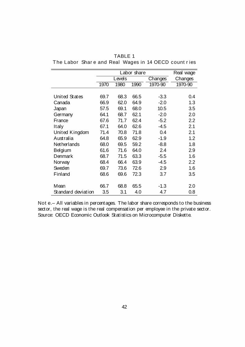
TABLE 1The Labor Share and Real Wages in 14 OECD countries

Labor share Real wageLevels Changes Changes

1970 1980 1990 1970-90 1970-90

United States 69.7 68.3 66.5 -3.3 0.4Canada 66.9 62.0 64.9 -2.0 1.3Japan 57.5 69.1 68.0 10.5 3.5Germany 64.1 68.7 62.1 -2.0 2.0France 67.6 71.7 62.4 -5.2 2.2Italy 67.1 64.0 62.6 -4.5 2.1United Kingdom 71.4 70.8 71.8 0.4 2.1Australia 64.8 65.9 62.9 -1.9 1.2Netherlands 68.0 69.5 59.2 -8.8 1.8Belgium 61.6 71.6 64.0 2.4 2.9Denmark 68.7 71.5 63.3 -5.5 1.6Norway 68.4 66.4 63.9 -4.5 2.2Sweden 69.7 73.6 72.6 2.9 1.6Finland 68.6 69.6 72.3 3.7 3.5

Mean 66.7 68.8 65.5 -1.3 2.0Standard deviation 3.5 3.1 4.0 4.7 0.8

Note.– All variables in percentages. The labor share corresponds to the businesssector, the real wage is the real compensation per employee in the private sector.Source: OECD Economic Outlook Statistics on Microcomputer Diskette.

42

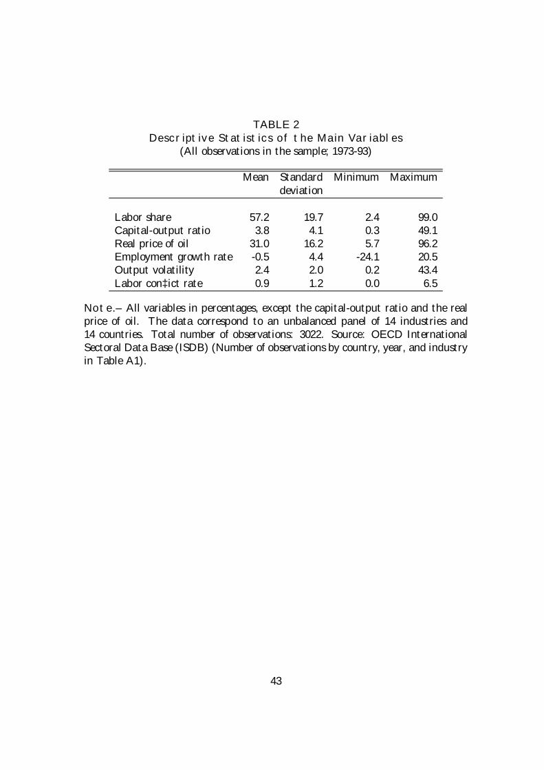
TABLE 2Descriptive Statistics of the Main Variables

(All observations in the sample; 1973-93)

Mean Standard Minimum Maximumdeviation

Labor share 57.2 19.7 2.4 99.0Capital-output ratio 3.8 4.1 0.3 49.1Real price of oil 31.0 16.2 5.7 96.2Employment growth rate -0.5 4.4 -24.1 20.5Output volatility 2.4 2.0 0.2 43.4Labor con‡ict rate 0.9 1.2 0.0 6.5

Note.– All variables in percentages, except the capital-output ratio and the realprice of oil. The data correspond to an unbalanced panel of 14 industries and14 countries. Total number of observations: 3022. Source: OECD InternationalSectoral Data Base (ISDB) (Number of observations by country, year, and industryin Table A1).

43

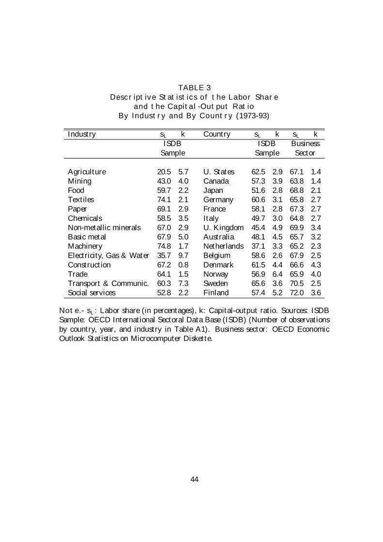
TABLE 3Descriptive Statistics of the Labor Share

and the Capital-Output RatioBy Industry and By Country (1973-93)

Industry sL k Country sL k sL kISDB ISDB Business

Sample Sample Sector

Agriculture 20.5 5.7 U. States 62.5 2.9 67.1 1.4Mining 43.0 4.0 Canada 57.3 3.9 63.8 1.4Food 59.7 2.2 Japan 51.6 2.8 68.8 2.1Textiles 74.1 2.1 Germany 60.6 3.1 65.8 2.7Paper 69.1 2.9 France 58.1 2.8 67.3 2.7Chemicals 58.5 3.5 Italy 49.7 3.0 64.8 2.7Non-metallic minerals 67.0 2.9 U. Kingdom 45.4 4.9 69.9 3.4Basic metal 67.9 5.0 Australia 48.1 4.5 65.7 3.2Machinery 74.8 1.7 Netherlands 37.1 3.3 65.2 2.3Electricity, Gas & Water 35.7 9.7 Belgium 58.6 2.6 67.9 2.5Construction 67.2 0.8 Denmark 61.5 4.4 66.6 4.3Trade 64.1 1.5 Norway 56.9 6.4 65.9 4.0Transport & Communic. 60.3 7.3 Sweden 65.6 3.6 70.5 2.5Social services 52.8 2.2 Finland 57.4 5.2 72.0 3.6

Note.- sL: Labor share (in percentages), k: Capital-output ratio. Sources: ISDBSample: OECD International Sectoral Data Base (ISDB) (Number of observationsby country, year, and industry in Table A1). Business sector: OECD EconomicOutlook Statistics on Microcomputer Diskette.

44

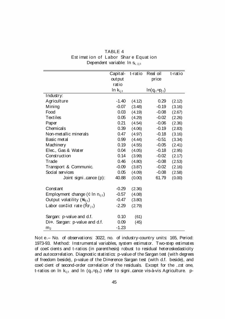
TABLE 4Estimation of Labor Share Equation

Dependent variable: ln sL;ijt

Capital- t-ratio Real oil t-ratiooutput priceratioln kijt ln(qjt=pjt)

Industry:Agriculture -1.40 (4.12) 0.29 (2.12)Mining -0.07 (3.48) -0.19 (3.16)Food 0.03 (4.19) -0.08 (2.67)Textiles 0.05 (4.29) -0.02 (2.26)Paper 0.21 (4.54) -0.06 (2.36)Chemicals 0.39 (4.06) -0.19 (2.83)Non-metallic minerals 0.47 (4.97) -0.18 (3.16)Basic metal 0.99 (4.44) -0.51 (3.34)Machinery 0.19 (4.55) -0.05 (2.41)Elec., Gas & Water 0.04 (4.05) -0.18 (2.95)Construction 0.14 (3.99) -0.02 (2.17)Trade 0.46 (4.80) -0.08 (2.53)Transport & Communic. -0.09 (3.87) -0.02 (2.16)Social services 0.05 (4.09) -0.08 (2.58)

Joint signi…cance (p): 40.88 (0.00) 61.79 (0.00)

Constant -0.29 (2.36)Employment change (¢ln nijt) -0.57 (4.08)Output volatility (e¾ijt) -0.47 (3.80)Labor con‡ict rate ( flcrjt) -2.29 (2.79)

Sargan: p-value and d.f. 0.10 (61)Di¤. Sargan: p-value and d.f. 0.09 (45)m2 -1.23

Note.– No. of observations: 3022, no. of industry-country units: 165, Period:1973-93. Method: Instrumental variables, system estimator. Two-step estimatesof coe¢cients and t-ratios (in parenthesis) robust to residual heteroskedasticityand autocorrelation. Diagnostic statistics: p-value of the Sargan test (with degreesof freedom beside), p-value of the Di¤erence Sargan test (with d.f. beside), andcoe¢cient of second-order correlation of the residuals. Except for the …rst one,t-ratios on ln kijt and ln (qjt=pjt) refer to signi…cance vis-à-vis Agriculture. p-

45

values of Wald test statistics of joint signi…cance of all ln kijt and ln (qjt=pjt) termsreported next to them. Instruments. (a) Di¤erences: di ln Kij;t¡2, (ln Kij;t¡2)2,¢ln nij;t¡2, e¾ijt, e¾ijt¡1, e¾ijt¡2, di flcrjt, and di ¢ln yj;t¡2. (b) Levels: di ¢ln kij;t¡2,¢e¾ijt, ¢e¾ijt¡1, ¢e¾ijt¡2, di ¢flcrjt, and di ¢2ln yj;t¡2.

46

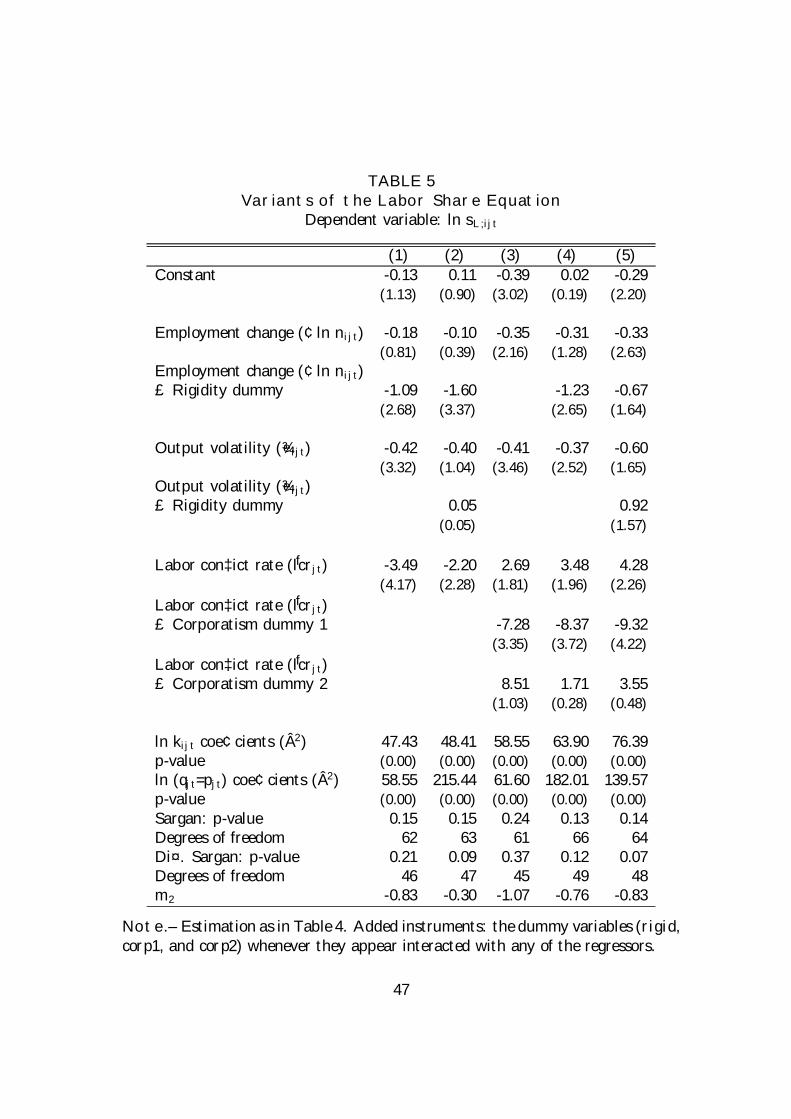
TABLE 5Variants of the Labor Share Equation

Dependent variable: ln sL;ijt

(1) (2) (3) (4) (5)Constant -0.13 0.11 -0.39 0.02 -0.29

(1.13) (0.90) (3.02) (0.19) (2.20)

Employment change (¢ln nijt) -0.18 -0.10 -0.35 -0.31 -0.33(0.81) (0.39) (2.16) (1.28) (2.63)

Employment change (¢ln nijt)£ Rigidity dummy -1.09 -1.60 -1.23 -0.67

(2.68) (3.37) (2.65) (1.64)

Output volatility (e¾ijt) -0.42 -0.40 -0.41 -0.37 -0.60(3.32) (1.04) (3.46) (2.52) (1.65)

Output volatility (e¾ijt)£ Rigidity dummy 0.05 0.92

(0.05) (1.57)

Labor con‡ict rate ( flcrjt) -3.49 -2.20 2.69 3.48 4.28(4.17) (2.28) (1.81) (1.96) (2.26)

Labor con‡ict rate ( flcrjt)£ Corporatism dummy 1 -7.28 -8.37 -9.32

(3.35) (3.72) (4.22)Labor con‡ict rate ( flcrjt)£ Corporatism dummy 2 8.51 1.71 3.55

(1.03) (0.28) (0.48)

ln kijt coe¢cients (Â2) 47.43 48.41 58.55 63.90 76.39p-value (0.00) (0.00) (0.00) (0.00) (0.00)ln (qjt=pjt) coe¢cients (Â2) 58.55 215.44 61.60 182.01 139.57p-value (0.00) (0.00) (0.00) (0.00) (0.00)Sargan: p-value 0.15 0.15 0.24 0.13 0.14Degrees of freedom 62 63 61 66 64Di¤. Sargan: p-value 0.21 0.09 0.37 0.12 0.07Degrees of freedom 46 47 45 49 48m2 -0.83 -0.30 -1.07 -0.76 -0.83

Note.– Estimation as in Table 4. Added instruments: the dummy variables (rigid,corp1, and corp2) whenever they appear interacted with any of the regressors.

47

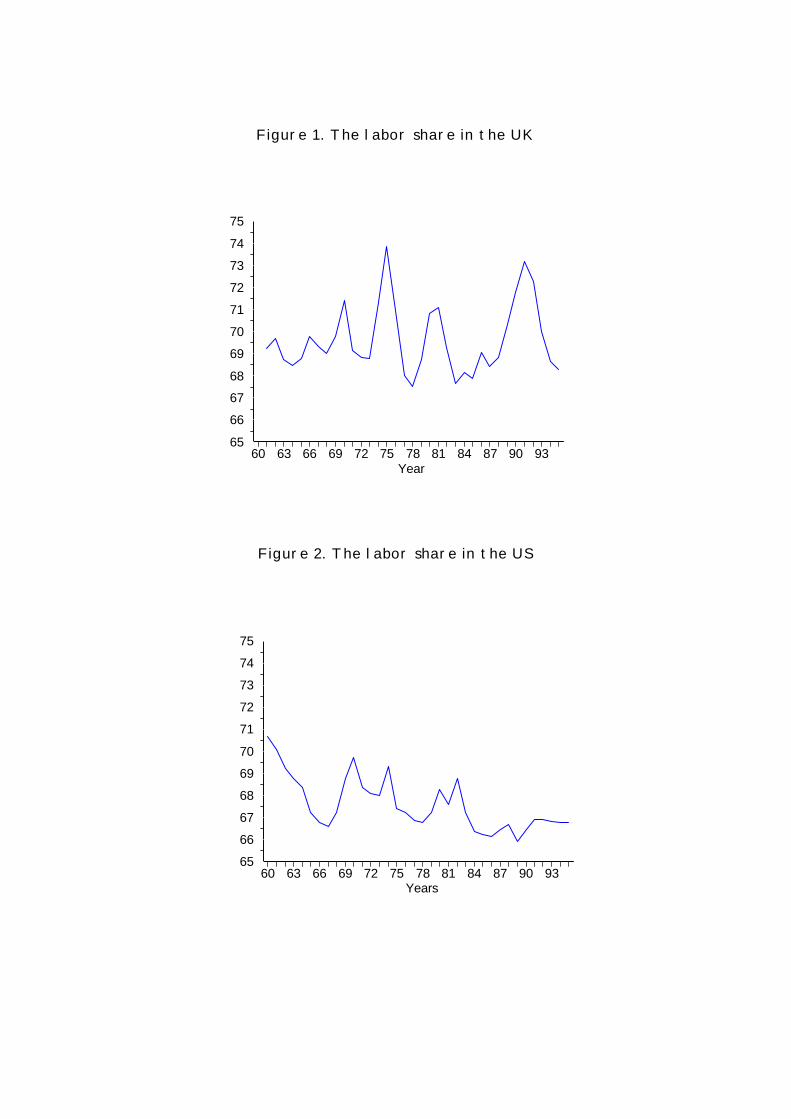
Figure 1. The labor share in the UK

Figure 2. The labor share in the US

65

66

67

68

69

70

71

72

73

74

75

60 63 66 69 72 75 78 81 84 87 90 93Year

65

66

67

68

69

70

71

72

73

74

75

60 63 66 69 72 75 78 81 84 87 90 93Years

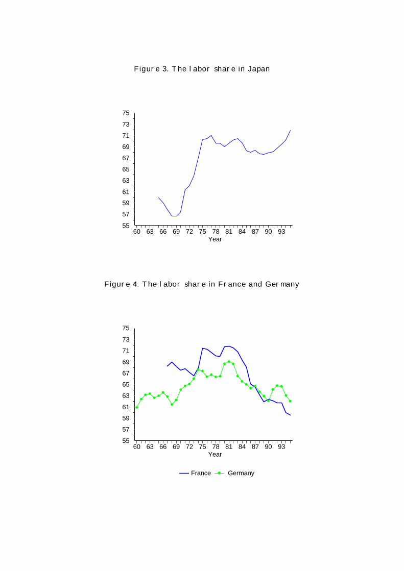
Figure 3. The labor share in Japan

Figure 4. The labor share in France and Germany

55

57

59

61

63

65

67

69

71

73

75

60 63 66 69 72 75 78 81 84 87 90 93Year

55

57

59

61

63

65

67

69

71

73

75

60 63 66 69 72 75 78 81 84 87 90 93Year

France Germany

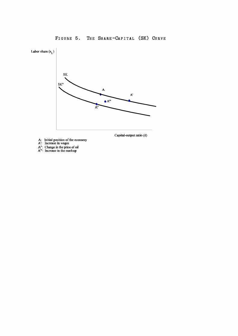
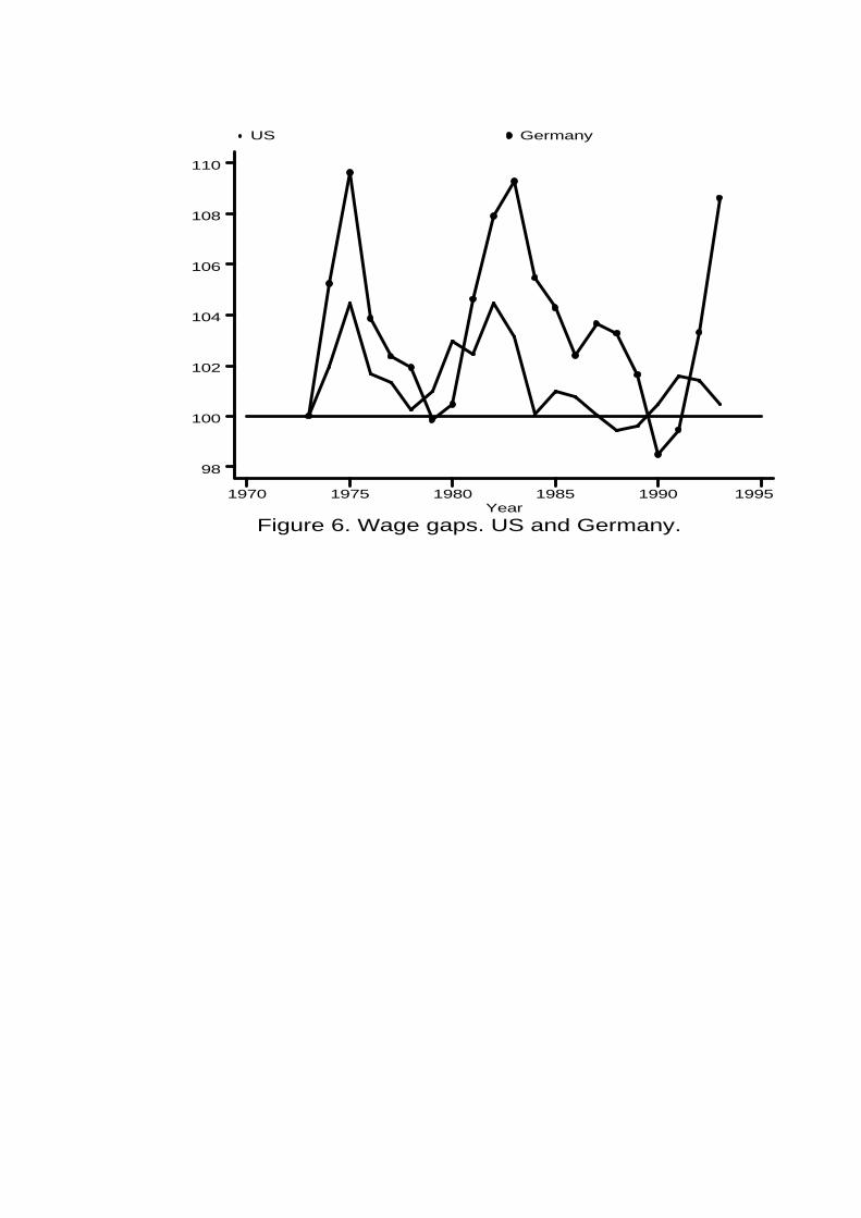
Figure 6. Wage gaps. US and Germany.Year

US Germany

1970 1975 1980 1985 1990 1995

98

100

102

104

106

108

110

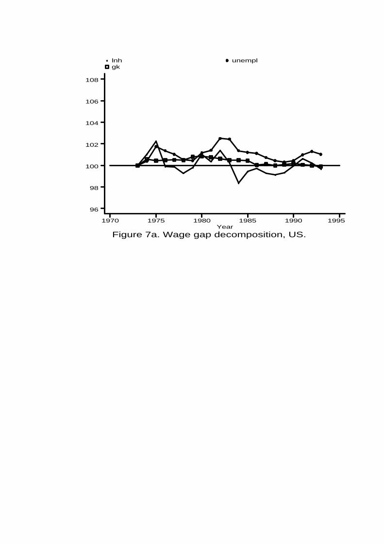
Figure 7a. Wage gap decomposition, US.Year

lnh unempl gk

1970 1975 1980 1985 1990 1995

96

98

100

102

104

106

108

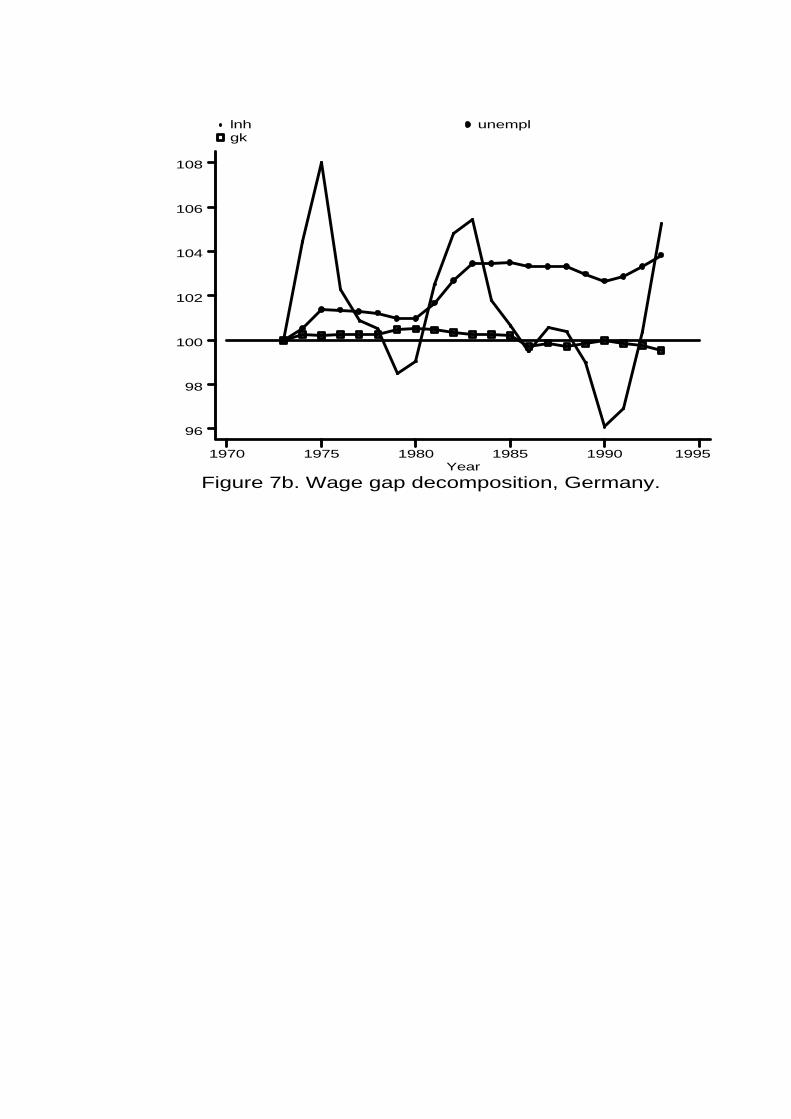
Figure 7b. Wage gap decomposition, Germany.Year

lnh unempl gk

1970 1975 1980 1985 1990 1995

96

98

100

102

104

106

108

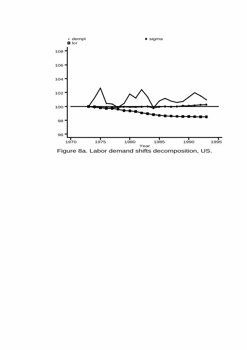
Figure 8a. Labor demand shifts decomposition, US.Year

dempl sigma lcr

1970 1975 1980 1985 1990 1995

96

98

100

102

104

106

108

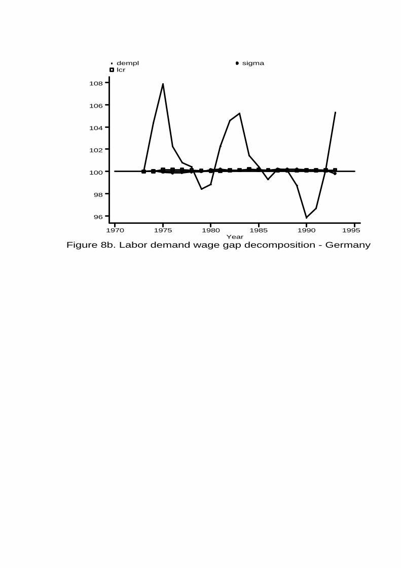
Figure 8b. Labor demand wage gap decomposition - GermanyYear

dempl sigma lcr

1970 1975 1980 1985 1990 1995

96

98

100

102

104

106

108