Embed Size (px)
Citation preview
Explaining the Italian GDP Using SpatialEconometrics
Carlos Hurtado
Department of EconomicsUniversity of Illinois at Urbana-Champaign
Junel 29th, 2016
C. Hurtado (UIUC - Economics) Spatial Econometrics
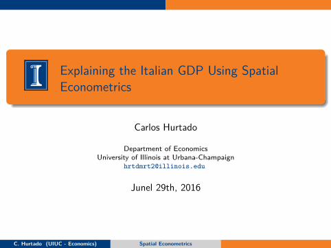
On the Agenda
1 Map of Italy and the W Matrix
2 The Italian GDP: A Simple Spatial Model
C. Hurtado (UIUC - Economics) Spatial Econometrics
Map of Italy and the W Matrix
On the Agenda
1 Map of Italy and the W Matrix
2 The Italian GDP: A Simple Spatial Model
C. Hurtado (UIUC - Economics) Spatial Econometrics
Map of Italy and the W Matrix
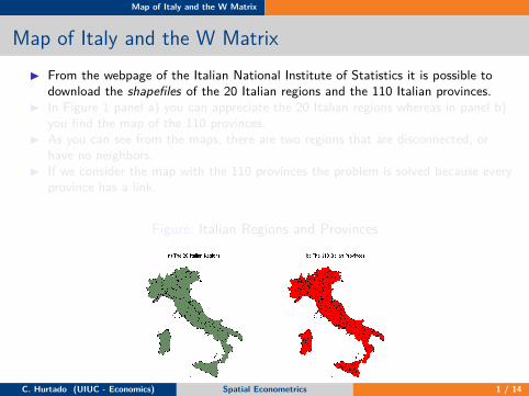
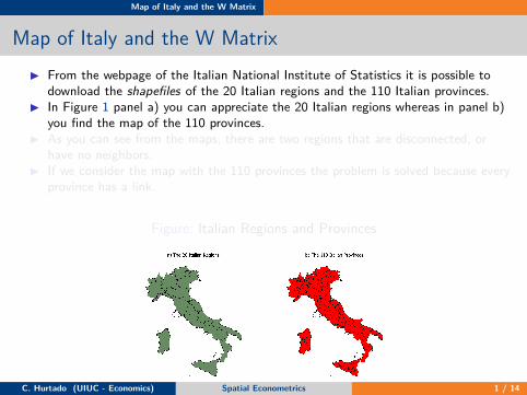
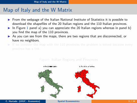
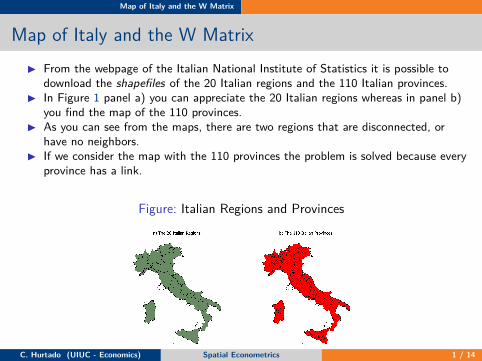
Map of Italy and the W MatrixI From the webpage of the Italian National Institute of Statistics it is possible to
download the shapefiles of the 20 Italian regions and the 110 Italian provinces.I In Figure 1 panel a) you can appreciate the 20 Italian regions whereas in panel b)
you find the map of the 110 provinces.I As you can see from the maps, there are two regions that are disconnected, or
have no neighbors.I If we consider the map with the 110 provinces the problem is solved because every
province has a link.
Figure: Italian Regions and Provinces
C. Hurtado (UIUC - Economics) Spatial Econometrics 1 / 14
Map of Italy and the W Matrix
Map of Italy and the W MatrixI From the webpage of the Italian National Institute of Statistics it is possible to
download the shapefiles of the 20 Italian regions and the 110 Italian provinces.I In Figure 1 panel a) you can appreciate the 20 Italian regions whereas in panel b)
you find the map of the 110 provinces.I As you can see from the maps, there are two regions that are disconnected, or
have no neighbors.I If we consider the map with the 110 provinces the problem is solved because every
province has a link.
Figure: Italian Regions and Provinces
C. Hurtado (UIUC - Economics) Spatial Econometrics 1 / 14
Map of Italy and the W Matrix
Map of Italy and the W Matrix
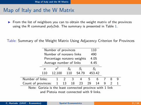
I From the list of neighbors you can to obtain the weight matrix of the provincesusing the R command poly2nb. The summary is presented in Table 1.
Table: Summary of the Weight Matrix Using Adjacency Criterion for Provinces
Number of provinces 110Number of nonzero links 490Percentage nonzero weights 4.05Average number of links 4.45
n n2 S0 S1 S2110 12,100 110 54.79 453.42
Number of links: 1 2 3 4 5 6 7 8 9Count of provinces: 1 13 18 23 29 14 9 2 1
Note: Gorizia is the least connected province with 1 linkand Pistoia most connected with 9 links.
C. Hurtado (UIUC - Economics) Spatial Econometrics 2 / 14
Map of Italy and the W Matrix
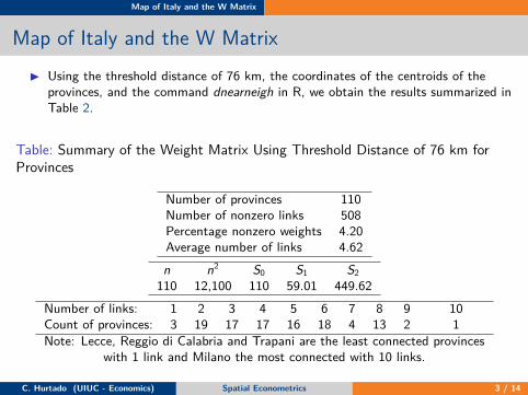
Map of Italy and the W MatrixI Using the threshold distance of 76 km, the coordinates of the centroids of the
provinces, and the command dnearneigh in R, we obtain the results summarized inTable 2.
Table: Summary of the Weight Matrix Using Threshold Distance of 76 km forProvinces
Number of provinces 110Number of nonzero links 508Percentage nonzero weights 4.20Average number of links 4.62
n n2 S0 S1 S2110 12,100 110 59.01 449.62
Number of links: 1 2 3 4 5 6 7 8 9 10Count of provinces: 3 19 17 17 16 18 4 13 2 1Note: Lecce, Reggio di Calabria and Trapani are the least connected provinces
with 1 link and Milano the most connected with 10 links.
C. Hurtado (UIUC - Economics) Spatial Econometrics 3 / 14
Map of Italy and the W Matrix
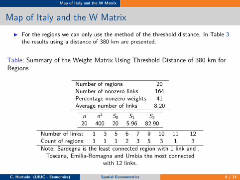
Map of Italy and the W MatrixI For the regions we can only use the method of the threshold distance. In Table 3
the results using a distance of 380 km are presented.
Table: Summary of the Weight Matrix Using Threshold Distance of 380 km forRegions
Number of regions 20Number of nonzero links 164Percentage nonzero weights 41Average number of links 8.20
n n2 S0 S1 S220 400 20 5.96 82.90
Number of links: 1 3 5 6 7 9 10 11 12Count of regions: 1 1 1 2 3 5 3 1 3Note: Sardegna is the least connected region with 1 link and ,
Toscana, Emilia-Romagna and Umbia the most connectedwith 12 links.
C. Hurtado (UIUC - Economics) Spatial Econometrics 4 / 14
Map of Italy and the W Matrix
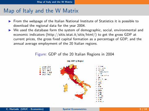
Map of Italy and the W MatrixI From the webpage of the Italian National Institute of Statistics it is possible to
download the regional data for the year 2004.I We used the database form the system of demographic, social, environmental and
economic indicators (http://sitis.istat.it/sitis/html/) to get the gross GDP atcurrent prices, the gross fixed capital formation as a percentage of GDP, and theannual average employment of the 20 Italian regions.
Figure: GDP of the 20 Italian Regions in 2004
C. Hurtado (UIUC - Economics) Spatial Econometrics 5 / 14
The Italian GDP: A Simple Spatial Model
On the Agenda
1 Map of Italy and the W Matrix
2 The Italian GDP: A Simple Spatial Model
C. Hurtado (UIUC - Economics) Spatial Econometrics
The Italian GDP: A Simple Spatial Model
Model Selection: Anselin’s method
C. Hurtado (UIUC - Economics) Spatial Econometrics 6 / 14
The Italian GDP: A Simple Spatial Model
Model Selection
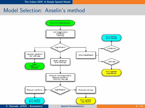
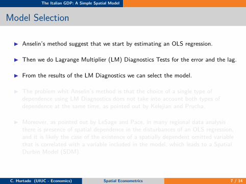
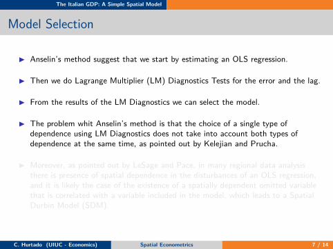
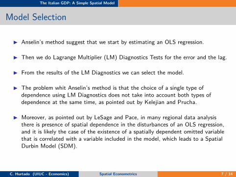
I Anselin’s method suggest that we start by estimating an OLS regression.
I Then we do Lagrange Multiplier (LM) Diagnostics Tests for the error and the lag.
I From the results of the LM Diagnostics we can select the model.
I The problem whit Anselin’s method is that the choice of a single type ofdependence using LM Diagnostics does not take into account both types ofdependence at the same time, as pointed out by Kelejian and Prucha.
I Moreover, as pointed out by LeSage and Pace, in many regional data analysisthere is presence of spatial dependence in the disturbances of an OLS regression,and it is likely the case of the existence of a spatially dependent omitted variablethat is correlated with a variable included in the model, which leads to a SpatialDurbin Model (SDM).
C. Hurtado (UIUC - Economics) Spatial Econometrics 7 / 14
The Italian GDP: A Simple Spatial Model
Model Selection
I Anselin’s method suggest that we start by estimating an OLS regression.
I Then we do Lagrange Multiplier (LM) Diagnostics Tests for the error and the lag.
I From the results of the LM Diagnostics we can select the model.
I The problem whit Anselin’s method is that the choice of a single type ofdependence using LM Diagnostics does not take into account both types ofdependence at the same time, as pointed out by Kelejian and Prucha.
I Moreover, as pointed out by LeSage and Pace, in many regional data analysisthere is presence of spatial dependence in the disturbances of an OLS regression,and it is likely the case of the existence of a spatially dependent omitted variablethat is correlated with a variable included in the model, which leads to a SpatialDurbin Model (SDM).
C. Hurtado (UIUC - Economics) Spatial Econometrics 7 / 14
The Italian GDP: A Simple Spatial Model
The Italian GDP: A Simple Spatial Model
I Let Y denote the gross GDP at current 2004 prices in billions of Euros, E denoteannual average of employed (in thousands), K denote the gross fixed capitalformation as percentage of GDP, and denoting by ε a well behaved Gaussian error.
C. Hurtado (UIUC - Economics) Spatial Econometrics 8 / 14
The Italian GDP: A Simple Spatial Model
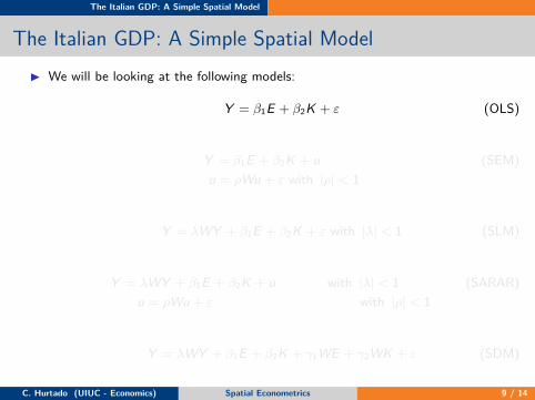
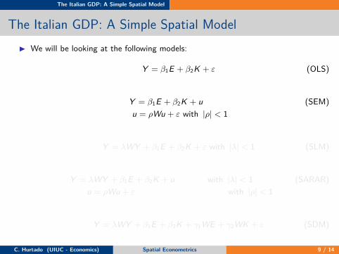
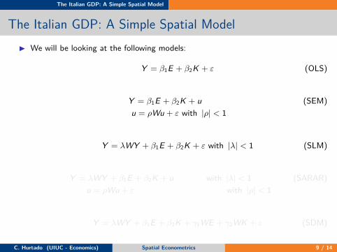
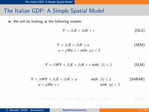
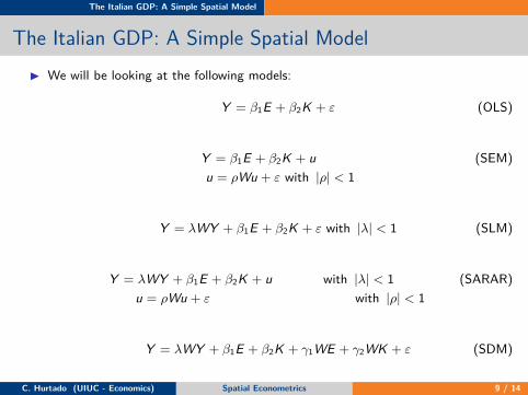
The Italian GDP: A Simple Spatial ModelI We will be looking at the following models:
Y = β1E + β2K + ε (OLS)
Y = β1E + β2K + u (SEM)u = ρWu + ε with |ρ| < 1
Y = λWY + β1E + β2K + ε with |λ| < 1 (SLM)
Y = λWY + β1E + β2K + u with |λ| < 1 (SARAR)u = ρWu + ε with |ρ| < 1
Y = λWY + β1E + β2K + γ1WE + γ2WK + ε (SDM)
C. Hurtado (UIUC - Economics) Spatial Econometrics 9 / 14
The Italian GDP: A Simple Spatial Model
The Italian GDP: A Simple Spatial ModelI We will be looking at the following models:
Y = β1E + β2K + ε (OLS)
Y = β1E + β2K + u (SEM)u = ρWu + ε with |ρ| < 1
Y = λWY + β1E + β2K + ε with |λ| < 1 (SLM)
Y = λWY + β1E + β2K + u with |λ| < 1 (SARAR)u = ρWu + ε with |ρ| < 1
Y = λWY + β1E + β2K + γ1WE + γ2WK + ε (SDM)
C. Hurtado (UIUC - Economics) Spatial Econometrics 9 / 14
The Italian GDP: A Simple Spatial Model
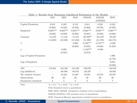
Table 1: Results from Maximum Likelihood Estimation of the ModelsOLS SEM SLM SARAR SARAR SDM
(GS2SLS)
Capital Formation 0.244 0.195 0.112 0.214 0.193 0.342
(0.605) (0.525) (0.532) (0.468) (0.579) (0.597)
Employed 0.063*** 0.063*** 0.064*** 0.064*** 0.064*** 0.065***
(0.002) (0.002) (0.002) (0.001) (0.002) (0.002)
Constant -12.470 -11.140 -17.274 -26.799** -24.153* -76.267
(14.630) (12.838) (13.188) (11.398) (14.178) (64.175)
λ 0.090 0.190*** 0.154*** -0.328
(0.062) (0.032) (0.048) (0.423)
ρ 0.260 -1.442*** -0.586
(0.347) (0.374) -
Lag of Capital Formation 1.808
(2.172)
Lag of Employed 0.034
(0.030)
AIC 141.681 143.180 141.340 136.670 - 144.010
Log Likelihood - -66.589 -65.672 -62.337 - -65.005
ML residual variance - 45.224 41.607 24.091 42.373 38.497
Observations 20 20 20 20 20 20
Parameters estimated 3 5 5 6 6 7
Note: ∗p < 0.1; ∗∗p < 0.05; ∗∗∗p < 0.01
OLS: Standard errors in parentheses
SEM, SLM, SARAR: Asymptotic standard errors in parentheses
SARAR (GS2SLS): GM standard errors in parentheses
SDM: Numerical Hessian approximate standard errors in parentheses
C. Hurtado (UIUC - Economics) Spatial Econometrics 10 / 14
The Italian GDP: A Simple Spatial Model
The Italian GDP: A Simple Spatial Model
I OLS model: Capital formation is not significant whereas employed is highlysignificant.
I Breusch–Pagan test has a p-value of 0.2451, and can not reject the null hypothesisof homoscedasticity in the residuals.
I Jarque-Bera test rejects with a significance level of 0.1 the null hypothesis ofnormality in the residuals (p-value = 0.09754)
I (SEM): LM Diagnostic for the error parameter tells us that we cannot reject thenull hypothesis of no spatial autocorrelation of the errors (p-value = 0.4487).
I (SLM): LM Diagnostic for the lag parameter rejects the null hypothesis of nospatially lagged dependent variable with a 0.1 significance level (p-value =0.09628).
I Following Anselin’s method we naively would have chosen SLM.
C. Hurtado (UIUC - Economics) Spatial Econometrics 11 / 14
The Italian GDP: A Simple Spatial Model
The Italian GDP: A Simple Spatial Model
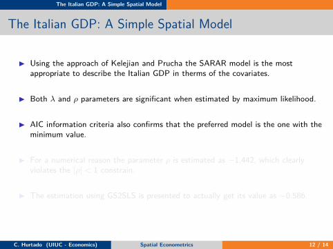
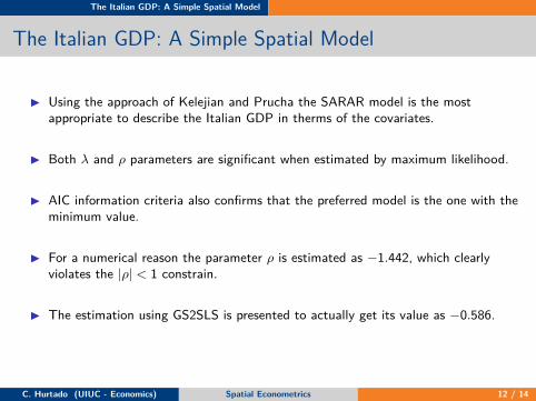
I Using the approach of Kelejian and Prucha the SARAR model is the mostappropriate to describe the Italian GDP in therms of the covariates.
I Both λ and ρ parameters are significant when estimated by maximum likelihood.
I AIC information criteria also confirms that the preferred model is the one with theminimum value.
I For a numerical reason the parameter ρ is estimated as −1.442, which clearlyviolates the |ρ| < 1 constrain.
I The estimation using GS2SLS is presented to actually get its value as −0.586.
C. Hurtado (UIUC - Economics) Spatial Econometrics 12 / 14
The Italian GDP: A Simple Spatial Model
The Italian GDP: A Simple Spatial Model
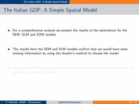
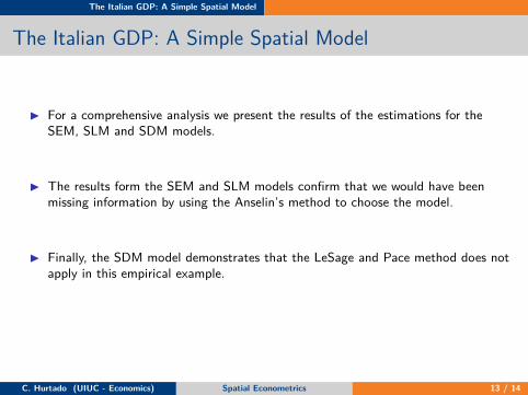
I For a comprehensive analysis we present the results of the estimations for theSEM, SLM and SDM models.
I The results form the SEM and SLM models confirm that we would have beenmissing information by using the Anselin’s method to choose the model.
I Finally, the SDM model demonstrates that the LeSage and Pace method does notapply in this empirical example.
C. Hurtado (UIUC - Economics) Spatial Econometrics 13 / 14
The Italian GDP: A Simple Spatial Model
The Italian GDP: A Simple Spatial Model
I For a comprehensive analysis we present the results of the estimations for theSEM, SLM and SDM models.
I The results form the SEM and SLM models confirm that we would have beenmissing information by using the Anselin’s method to choose the model.
I Finally, the SDM model demonstrates that the LeSage and Pace method does notapply in this empirical example.
C. Hurtado (UIUC - Economics) Spatial Econometrics 13 / 14
The Italian GDP: A Simple Spatial Model
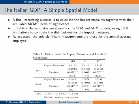
The Italian GDP: A Simple Spatial ModelI A final interesting exercise is to calculate the impact measures together with their
simulated MCMC levels of significance.I In Table 2 the estimates are shown for the SLM and SDM models, using 1000
simulations to compute the distributions for the impact measures.I As expected, the only significant measurements are those for the annual average
employed.
Table 1: Estimates of the Impact Measures and Levels ofSignificance
ADI AII ATI
SLM
Capital Formation 0.1126 0.0110 0.1235
(0.2620) (0.1463) (0.2549)
Employed 0.0638*** 0.0062 0.0700***
(37.98) (1.34) (12.64)
SDM
Capital Formation 0.2825 1.3374 1.6199
(0.4258) (0.7093) (0.7401)
Employed 0.0645*** 0.0102* 0.0747***
(36.91) (1.66) (10.42)
Note: ∗p < 0.1; ∗∗p < 0.05; ∗∗∗p < 0.01
Simulated z-values in parentheses
C. Hurtado (UIUC - Economics) Spatial Econometrics 14 / 14


![Explaining brightness illusions using spatial filtering · PDF fileExplaining brightness illusions using spatial filtering ... 1979, 413]. Our models extend Blakeslee and McCourt](https://img.pdfslide.net/doc/110x75/5aa3e2e07f8b9a07758ed3b1/explaining-brightness-illusions-using-spatial-ltering-brightness-illusions.jpg)