Embed Size (px)
Citation preview

1
The Version of Record of this manuscript has been published and is available in Forest Science, Volume 59, Number 2, 2013, pp. 211-222.
Published: 01 April 2013 DOI: http://dx.doi.org/10.5849/forsci.11-078
Explaining the Shifts of International Trade in Pulp and Paper Industry
Maija Hujalaa*, Heli Arminena, R. Carter Hillb, Kaisu Puumalainena
aSchool of Business, Lappeenranta University of Technology, P.O. Box 20, FIN-53851, Lappeenranta, Finland b Louisiana State University, Economics Department, 2317 Business Education Complex, Baton Rouge, LA 70803 *Corresponding author E-mail address: [email protected] (M. Hujala)
Abstract
The pulp and paper industry is currently facing broad structural changes due to global shifts in
demand and supply. These changes have significant impacts on national economies worldwide. In
this paper, we describe the recent trends in the pulp and recovered paper (RP) production, and
estimate augmented gravity models of bilateral trade for chemical pulp and RP exports with panel
data. According to our results, there is some variation in the effects of the traditional gravity-model
variables between pulp grades and RP. The results imply also that, in comparison to export supply,
import demand plays a larger role in determining the volume of exports. Finally, it is evident that
Asia, particularly China, is the most important driver of chemical pulp and RP trade: China is
hungry for fiber, and must import to satisfy its growing needs. Moreover, the speed of China’s
growth in chemical pulp and RP imports has been driving the increased significance of planted
forests in the exports of hardwood pulp (BHKP) as well.
Keywords: Pulp and paper industry; bilateral trade; gravity model of international trade; panel
data; Hausman-Taylor estimator
JEL Classifications: C23, F11, Q23, Q27
2
Introduction
The input and output markets of the pulp and paper industry (P&PI) are experiencing dramatic
structural changes (e.g. McCarthy and Lei 2010, Toppinen and Kuuluvainen 2010, Hetemäki 2005
p. 97). These shifts include, among others, the substitution of printed media for electronic
communication technologies, the shift in advertising expenditures from print media to electronic
media, the liberalization of trade with formerly closed low-income economies such as China, and
the increased importance of planted forests and recovered paper as a raw material for paper
production. Until the late 1980s, the global pulp production was centered in the northern
hemisphere, especially in North America and Northern Europe. More recently, due to innovations
in clonal forestry and pulp and paper processes, also the eucalyptus tree has become an important
raw material in paper production (Figueiredo 2010). At the present, eucalyptus pulp is in great
demand as a raw material especially for fine papers. During the past decade, Latin America
(particularly Brazil) with its enormous eucalyptus plantations has become one of the most
important hardwood pulp producers although its domestic demand for pulp is low in comparison
to, for example, North America and Western Europe.
Together with the global shifts in pulp markets, the focal point of paper and paperboard
manufacturing has moved closer to rapidly growing markets in Asia, particularly in China. In the
traditional paper production areas, i.e. North America and Western Europe, paper demand is
stagnating or even decreasing, depending on the paper grade, and as a consequence the number of
pulp and paper machines and mills has declined dramatically in the recent years. Also, increasing
demand for paper and paperboard as well as growing environmental awareness have boosted the
use of recovered paper (hereafter RP) as a raw material in paper production during the past decades.

3
According to the United Nation’s Food and Agriculture Organization’s ForesSTAT database (FAO
2011a), the use of recovered fiber exceeds nowadays the use of virgin fiber as a raw material.
All the changes in input and output markets have affected the trade of raw materials for paper and
paperboard via changes in their import demand and export supply [1]. A tool frequently used to
evaluate export and import flows is the gravity model of international trade. The model has been
used also in the context of forest products trade (e.g. Kangas and Niskanen 2003, Polyakov and
Teeter 2007, Zhang and Li 2009) but only for limited geographic areas and/or with cross-sectional
data. Despite the significant impacts that the dynamic changes in P&PI have on national economies
worldwide, the subject has hardly been studied by using global data and advanced panel data
estimation methods. Our aim is to fill this gap.
The objective of this paper is to model bilateral trade patterns of chemical pulp and RP. We first
describe the recent trends in global wood pulp and RP markets and then empirically examine
bilateral trade flows of bleached kraft pulp and RP. We draw from the theories of the gravity model
and international trade, and estimate an extended gravity model with measures of import demand
and export supply as explanatory variables. Analyses are done using the generalized instrumental
variable estimator of Hausman and Taylor (1981) with panel data between 1990 and 2008.
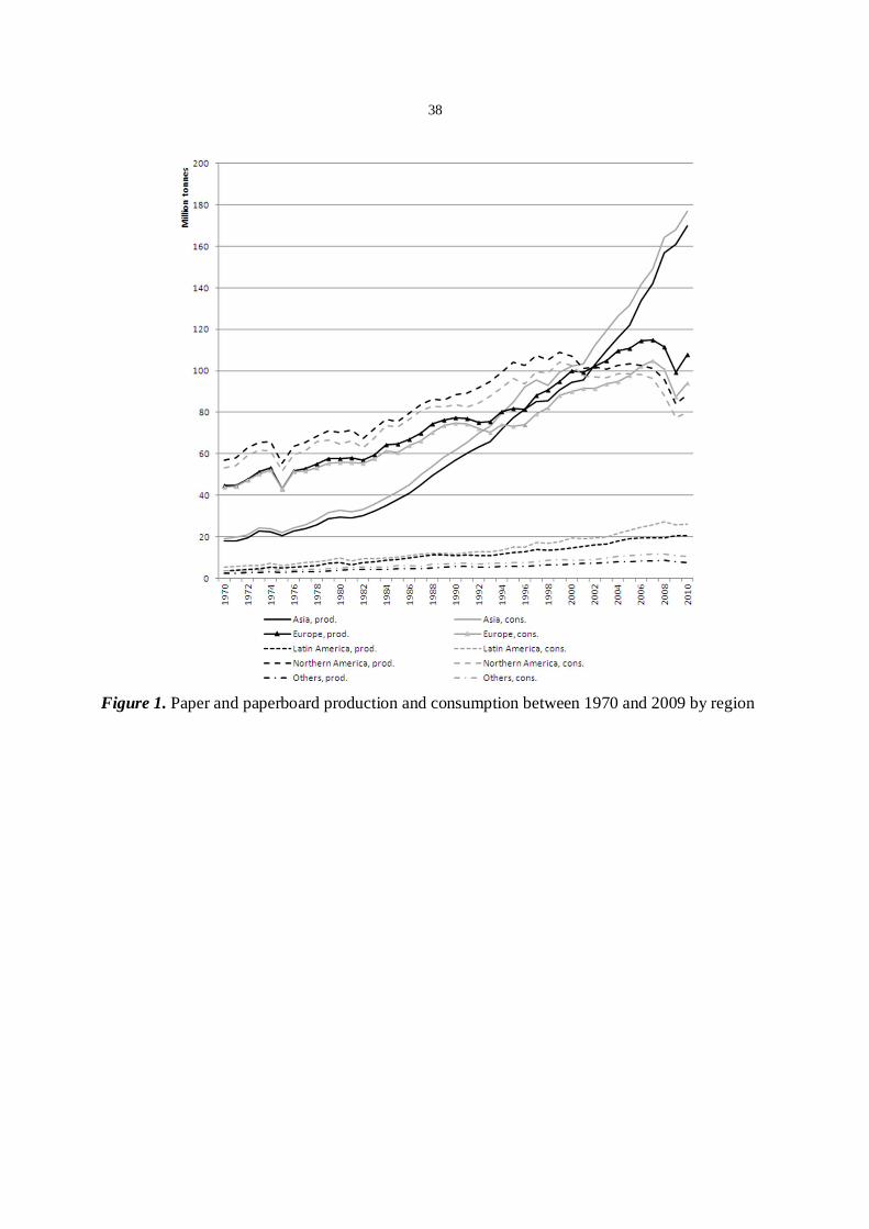
Global Paper and Pulp Markets
Since 1970, the total consumption of paper and paperboard has tripled and was over 377 million
tonnes in 2009 (FAO 2011a). However, there are massive differences between regions in the pace
of demand growth and the phase of the industry life cycle. As shown in Figure 1, Europe and North

4
America dominated paper and paperboard production and consumption until the 1990s. In North
America, the markets matured in the early 1990s and consumption, as well as production, has
mainly decreased since 2000. In Europe, consumption and production reached the maximum in
2007 and started to decline after that. One reason for the decrease in North American and Western
European paper markets is the substitution effect of electronic media (see for example Hetemäki
2005, Hujala 2011). Respectively, one of the most significant causes for the stagnating demand for
paperboard in developed countries is the globalization of manufacturing industries (Diesen 2007 p.
38). In other words, as manufacturing industries have moved parts of their production from
industrialized countries to, for example, China, the need for packaging paper and paperboard has
declined in Western markets.
In Asia, the demand for paper has been boosted by economic growth since the early 1980s and the
region contributes nowadays over 40 percent of the total paper and paperboard consumption. Asia
has been a net importer throughout the period, while North America and lately especially Europe
have been the largest net exporters. Latin America only accounts for about 3 percent of the global
production and consumption of paper. In 2009, the largest paper and paperboard
consumers/producers were China (86.4/85.7 million tonnes), United States (71.6/71.7 million
tonnes), and Japan (26.3/27.3 million tonnes) (RISI 2011a). As shown in Figure 1, production and
consumption series for paper and paperboard are almost identical, indicating that paper production
has been, and still is, located near the markets.
[Place Figure 1 approximately here]

5
The most important raw materials in paper and paperboard production are wood pulp and recovered
paper. Figure 2 depicts the production (i.e. recovery) of RP and wood pulp by grade [2]. As shown,
the production of RP is skyrocketing, making it the fastest-growing raw material in paper industry.
The world’s waste paper recovery increased by 490 percent between 1970 (30.8 million tonnes)
and 2009 (182 million tonnes). Some of the most important factors that have influenced the demand
for recovered fiber in P&PI positively include: 1) insufficient virgin pulp and RP fiber supply in
Asia along with the region’s (and particularly China’s) growing fiber consumption, 2) increased
demand for all raw materials, 3) technological progress in the areas of, for example, deinking and
screening of impurities (Diesen 2007 p. 81), 4) good price competitiveness in comparison to virgin
fiber, and 5) increased environmental awareness (Hujala et al. 2010).
Figure 2 also shows how the production of chemical pulp almost doubled between 1970 (65.8
million tonnes) and 2009 (119 million tonnes). Instead, the manufacturing of mechanical pulp
increased until 1990 but has stagnated since then, being 28.5 million tonnes in 2009 (about one
fourth of the production of chemical pulp). Mechanical pulp is used largely for products like
newsprint and mechanical papers, the use of which is declining in North America and Western
Europe due to the increased popularity of electronic media. Moreover, several closures of
mechanical paper machines and mills in Finland and elsewhere in Western Europe cut overcapacity
in 2008 (Valtonen 2008 p. 21). In Asia, growing paper demand has boosted the use of RP and
chemical pulp instead of mechanical pulp because the production of mechanical pulp is typically
integrated with paper production. According to the Mill Project database provided by RISI (2011b)
[3], several new mechanical pulp lines and pulp mills have been established in China since 2004,
but the region’s mechanical pulp production capacity still falls short of fulfilling paper mills’ needs.
Recycled fiber can be used to make largely same end products as mechanical pulp, but it is usually
6
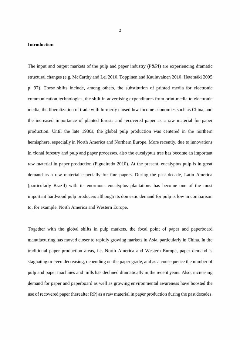
impossible to use RP as a substitute for chemical pulp. Therefore, increases in Asia’s paper
production have required higher RP and chemical pulp imports to the area, because of which the
global RP and chemical pulp output has increased. Semi-chemical pulp has been less important in
world-scale paper and paperboard manufacturing (9.15 million tonnes in 2009). However, its
production shows a slightly increasing trend after the late 1990s.
[Place Figure 2 approximately here]
Market pulp (i.e. pulp sold and bought on the open market) is mainly chemical pulp. In 2009,
chemical pulp exports were about 40 million tonnes in total, almost thirteen times those of
mechanical pulp. Figures 3 and 4 show the production and consumption of RP and chemical pulp
by region.
[Place Figure 3 approximately here]
[Place Figure 4 approximately here]
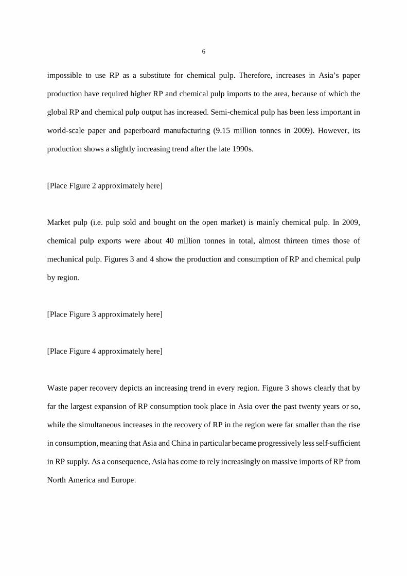
Waste paper recovery depicts an increasing trend in every region. Figure 3 shows clearly that by
far the largest expansion of RP consumption took place in Asia over the past twenty years or so,
while the simultaneous increases in the recovery of RP in the region were far smaller than the rise
in consumption, meaning that Asia and China in particular became progressively less self-sufficient
in RP supply. As a consequence, Asia has come to rely increasingly on massive imports of RP from
North America and Europe.

7
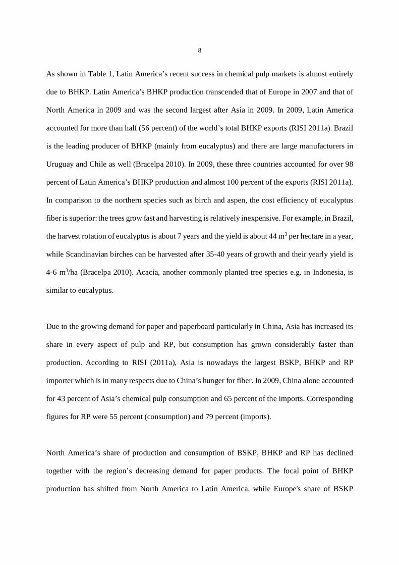
As depicted in Figure 4, North American and European chemical pulp production has stagnated or
decreased during the past years, reflecting the maturity of the paper products markets in these
regions. Nevertheless, these two areas are still the largest chemical pulp producers. However, Latin
America has rapidly gained a position as a major player in the global pulp industry: the total
chemical pulp production of the area almost doubled between 2002 and 2009. In addition, more
than half of the production was exported in 2009. In contrast, Asia is increasingly less self-
sufficient in chemical pulp, and relies on larger volumes of imports from the other world regions,
especially from Latin America.
Chemical pulp can be divided further into bleached softwood kraft pulp (BSKP), bleached
hardwood kraft pulp (BHKP), unbleached kraft pulp and sulfite pulp (unbleached and bleached).
“Kraft” refers to sulfate pulping process and “hardwood” and “softwood” to the raw material.
Softwood is wood from conifers (for example pines and spruces) while hardwood comes from
broad-leaved trees such as acacia, birch and eucalyptus. According to the RISI’s Industry Statistics
database, chemical pulp exports consist mainly of BHKP (19.9 million tonnes and 49.9 percent of
the total chemical pulp exports in 2009) and BSKP (17.5 million tonnes and 43.8 percent in 2009).
In turn, RP exports were over 55 million tonnes. Thus, the three most exported raw materials in
P&PI are RP, BHKP and BSKP. As shown in Figures 3 and 4, production of market pulp and RP
is not necessarily located near consumption (unlike with paper and paperboard). Table 1 shows the
percentages of the global production and consumption for the three raw materials by region.
[Place Table 1 approximately here]
8
As shown in Table 1, Latin America’s recent success in chemical pulp markets is almost entirely
due to BHKP. Latin America’s BHKP production transcended that of Europe in 2007 and that of
North America in 2009 and was the second largest after Asia in 2009. In 2009, Latin America
accounted for more than half (56 percent) of the world’s total BHKP exports (RISI 2011a). Brazil
is the leading producer of BHKP (mainly from eucalyptus) and there are large manufacturers in
Uruguay and Chile as well (Bracelpa 2010). In 2009, these three countries accounted for over 98
percent of Latin America’s BHKP production and almost 100 percent of the exports (RISI 2011a).
In comparison to the northern species such as birch and aspen, the cost efficiency of eucalyptus
fiber is superior: the trees grow fast and harvesting is relatively inexpensive. For example, in Brazil,
the harvest rotation of eucalyptus is about 7 years and the yield is about 44 m3 per hectare in a year,
while Scandinavian birches can be harvested after 35-40 years of growth and their yearly yield is
4-6 m3/ha (Bracelpa 2010). Acacia, another commonly planted tree species e.g. in Indonesia, is
similar to eucalyptus.
Due to the growing demand for paper and paperboard particularly in China, Asia has increased its
share in every aspect of pulp and RP, but consumption has grown considerably faster than
production. According to RISI (2011a), Asia is nowadays the largest BSKP, BHKP and RP
importer which is in many respects due to China’s hunger for fiber. In 2009, China alone accounted
for 43 percent of Asia’s chemical pulp consumption and 65 percent of the imports. Corresponding
figures for RP were 55 percent (consumption) and 79 percent (imports).
North America’s share of production and consumption of BSKP, BHKP and RP has declined
together with the region’s decreasing demand for paper products. The focal point of BHKP
production has shifted from North America to Latin America, while Europe's share of BSKP

9
production has expanded (this is most likely due to the negative development in North America).
Europe’s significance in both BHKP and BSKP consumption remained roughly the same between
1992 and 2009. Also Europe’s share of RP production has held at about 30 percent of the total
production.
Discussion based on figures and tables is always only descriptive by nature, but we are also
interested in the statistical significance of the phenomena. Moreover, the investigation of the
relations between the ongoing dynamic changes in P&PI requires econometric analysis. We next
proceed to the description of the research methodology and then use gravity models of international
trade to explain shifts in the exports of BSKP, BHKP and RP.
Research Methodology
Gravity Models of International Trade
Gravity models of international trade predict that the flow of commodities between two countries
is positively related to their size and negatively related to their distance. Over time, other
explanatory variables have been added into the models to capture the effects of the supply and
demand conditions in the exporter and the importer. Gravity models have been used extensively in
the literature of international trade to evaluate the impacts of trade liberalization and preferential
trading agreements, to predict trade potentials of countries and to give policy prescriptions.
Tinbergen (1962) and Pöyhönen (1963) first introduced the gravity model in this context, while
Linnemann (1966) augmented their work. In the simplest form of the model,
ijij
ijjijiij
XDPOPPOPGDPGDPT
6
543210 lnlnlnlnlnln
(1)

10
the volume of trade T is defined by supply conditions in the exporting country i (GDP and
population), demand conditions in the importing country j (GDP and population) as well as
bilateral trade resistance factors (transport costs approximated by geographical distance D), and
trade preference factors Xij (e.g. common border and preferential trading agreements). Some
authors (e.g. Serlenga and Shin 2007) drop population from equation (1) to avoid multicollinearity.
In addition, Anderson and van Wincoop (2003) stress that the volume of trade between any two
countries also depends on what they call “multilateral trade resistance”, i.e. factors that impact on
how difficult it is for the countries to trade with the rest of the world. High multilateral resistance
in either of the countries increases the bilateral trade volume.
The early contributions to explaining the volume of trade via gravity models were criticized for not
having a proper theoretical foundation. However, it has later been demonstrated that the predictions
of the models can be derived from various models of international trade, including Ricardian,
Heckscher-Ohlin and increasing-returns-to-scale models (see for example the seminal paper by
Anderson 1979, and Bergstrand 1985, 1989, 1990, Helpman and Krugman 1985, Deardorff 1998,
and Anderson and van Wincoop 2003). Therefore, the gravity model does not rule out the theory
of comparative advantage but can actually be derived from it.
Although the bulk of the research analyzes the volume of aggregate trade (or exports or imports),
some studies focus on the sectoral level (Fernandes 2006, Vicarelli et al. 2008). Even more
disaggregated data can be used. Koo and Karemera (1991) and Koo et al. (1994) revise the gravity
model of trade for a single commodity, demonstrating that gravity models can also be applied to
single commodity markets: Koo and Karemera analyze wheat trade, while Koo et al. investigate
the trade of meat. In the same spirit, Dascal et al. (2002) estimate gravity equations for EU wine
11
exports and imports, and Amponsah and Ofori-Boadu (2006) analyze textile and apparel imports
to United States from the key trading partners. Kangas and Niskanen (2003), Välikauppi et al.
(2006), Polyakov and Teeter (2007), Zhang and Li (2009), and Akyüz et al. (2010) use gravity
models in the context of forest products trade. Analyzing the trade of a single commodity means
that it is important to include regressors that impact on the supply and demand of that commodity,
therefore affecting its export supply and import demand. Thus, Dascal et al. (2002) include
production indices of wine in their gravity equation, while Koo et al. (1994) control for the number
of animals in exporting and importing countries to measure livestock production capacity.
Polyakov and Teeter (2007) use data on production (supply) and consumption (demand) of
pulpwood as the determinants of export supply and, respectively, import demand. In another recent
paper, Zhang and Li (2009) explain China’s wood products trade with roundwood production (per
capita) and Chinese logging restrictions as the measures of export supply and import demand.
Augmented Gravity Model for Pulp Trade
In this paper, we examine the bilateral trade flows of the three most exported raw materials in the
global paper and paperboard production: BSKP, BHKP and RP. We extend the basic gravity model
with some explanatory variables reflecting the supply and demand conditions in the exporter and
the importer, because these contribute to export supply and import demand. As Polyakov and
Teeter (2007) highlight, this is necessary when applying the gravity model to a single commodity
market. The specifications of our full gravity equation are as follows [4]:
1) BSKP and RP (for RP without FAit)

12
.
121110987
654321
54321
ln
lnlnlnlnlnln
lnln
ijtij
jtititittijt
jtitjtitjt
jt
it
it
jiiiijijt
DECCHNDECNEDECLADECNADECRER
FAFAPOPPOPPOPGDP
POPGDP
CHNNELANADT
(2)
2) BHKP
.10987
654321
321
ln
lnlnlnlnlnln
lnln
ijtijjtittijt
jtitjtitjt
jt
it
it
jiijijt
DECCHNDECPFDECRER
FAFAPOPPOPPOPGDP
POPGDP
CHNPFDT
(3)
Our dependent variable Tijt is pulp exports (BSKP, BHKP or RP) from country i to country j in
year t. The regressors common to all models include distance (D), importer dummy for China
(CHN), level of economic development (GDP/POP), population (POP), raw material resources
(FA, forest area), bilateral real exchange rate (RER), decade dummy (DEC) and the interaction of
China and decade dummies (DECCHN). In addition, equation (2) for BSKP and RP incorporates
exporter dummies [5] for North America (NA), Latin America (LA) and North Europe (NE) as well
as the interactions of the exporter and decade dummies (DECNA, DECLA, DECNE) in the model.
In contrast, equation (3) for BHKP includes a dummy for planted forests of eucalyptus and acacia
(PF) [6] and the interaction of this variable and the decade dummy (DECPF). All variables apart
from the dummy variables are expressed in logs. Regression coefficients are assumed to be
common to all country pairs. The term ij represents country-pair effects [7] and captures such
time-invariant factors that are not included in the model. Finally, ijt is the error term, which is
assumed homoscedastic and serially uncorrelated.

13
Common border and common language dummies are often included in gravity models as trade-
aiding factors. We exclude these variables due to the nature of our dependent variables. BSKP,
BHKP and RP are bulk products usually traded between rather large companies, indicating that
common language and border do not have a significant impact on the volume of trade. Also relative
production costs might impact on export supply and import demand of pulp. However, these tend
to correlate so strongly with GDP per capita that both variables cannot be included in the model.
As is commonly done in the literature, distance D is measured by the distance between the capitals
of the bilateral trade pairs (see e.g. Egger 2002). Head and Mayer (2010) discuss the issue of
choosing the appropriate measure of distance. Because distance is a proxy for transport costs, it
should reduce the volume of exports. The expected sign of 1 is thus negative.
Exporter’s gross domestic product (GDP) per capita GDPi/POPi, population POPi and forest area
FAi impact on the export supply of BSKP and BHKP and, respectively, GDPj/POPj, POPj and FAj
affect the importer’s import demand. Although modern information and communication
technologies, especially internet, reduce the consumption of printing and writing papers, the level
of economic development (measured by GDP per capita) still determines the volume of paper
consumption in most countries (Hetemäki 2005 p. 77, McCarthy and Lei 2010, Hujala 2011). In
comparison to less developed countries, economically developed countries have stronger domestic
(per capita) demand for paper. Also population growth increases the demand for paper. As rising
domestic demand for paper-based products depresses export supply of pulp and increases its import
demand, we expect and to be negative and and to be positive with BSKP and BHKP.
With RP, we expect and to be positive as well. Instead, the expected signs of and are
14
not clear because the influence of GDP per capita on domestic demand of RP is twofold. First, the
higher the domestic demand for paper products is (i.e. the higher the country’s GDP per capita is),
the higher is the demand for RP as raw material. Second, at the same time, the supply of waste
paper to be recovered (and exported) is higher as well.
Forest area FA (in km2) measures the long-run availability of raw material for pulp. With BSKP
and BHKP, an increase in the exporter’s forest area FAi should boost export supply. On the other
hand, BHKP exports are largely dominated by Brazil (about 7 million tonnes in 2008) and
Indonesia (about 2.6 million tonnes in 2008), both of which suffer from severe deforestation (see
e.g. FAO 2011b). Because FA measures the total area of forested land, not only commercial or
planted forests, this might result in a negative coefficient for exporter’s forest area in the case of
BHKP. With RP, we exclude FAi from the model because the raw material for RP is paper, not
wood. The coefficient of FAj is expected to be negative, as paper-producing countries with smaller
forest resources need to import pulp and RP from elsewhere.
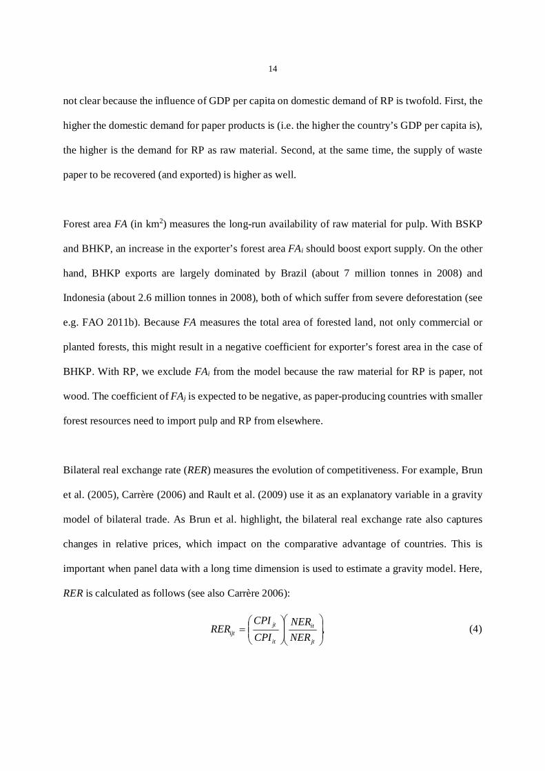
Bilateral real exchange rate (RER) measures the evolution of competitiveness. For example, Brun
et al. (2005), Carrère (2006) and Rault et al. (2009) use it as an explanatory variable in a gravity
model of bilateral trade. As Brun et al. highlight, the bilateral real exchange rate also captures
changes in relative prices, which impact on the comparative advantage of countries. This is
important when panel data with a long time dimension is used to estimate a gravity model. Here,
RER is calculated as follows (see also Carrère 2006):
,jt
it
it
jtijt NER
NERCPICPI
RER (4)
15
where CPI is the consumer price index and NER the nominal exchange rate against USD (local
currency units per United States dollar). A depreciation of the exporter’s currency against that of
the importer improves the competitiveness of the exporter and leads to an increase in RER. We thus
expect the coefficient of RER to be positive.
The interactions of the area dummies with the decade dummy (DECNA, DECLA, DECNE and
DECCHN) capture such additional variation in the trade flows that cannot be explained by the other
explanatory variables. Exporter and China dummies were chosen on the grounds of the analysis of
global pulp and paper markets presented earlier. Exporter dummies NA, LA and NE equal one if
the exporting country is situated in the geographic area in question, 0 otherwise. China dummy
CHN equals one when China is the importing country. Decade dummy DEC equals one if the year
> 2000, and interaction terms DECNA, DECLA, DECNE and DECCHN combine the region and
decade dummies. Thus, DECNA, DECLA and DECNE equal one if the exporter is situated in that
region and year > 2000 and, respectively, DECCHN equals 1 if China is the importer and year >
2000. China’s growing role in the world trade should be visible in the imports of BSKP, BHKP
and RP. In addition, we expect to observe the increased importance of planted eucalyptus and
acacia forests for BHKP exports in the 2000s via a positive coefficient of DECPF.
Data Description
The data for this study were collected from various sources. The data on paper and paperboard,
wood pulp, RP and chemical pulp production and consumption from 1970 to 2009 are from the
ForesSTAT database provided by the UN’s Food and Agriculture organization (FAO) (FAO
2011a). The data on production, consumption and trade of BSKP, BHKP and RP between 1992
and 2009 originate from the Industry Statistics database of RISI (RISI 2011a). The annual bilateral

16
trade flows of BSKP, BHKP and RP between 1990 and 2008 come from RISI as well. GDPs,
populations, forest areas, official exchange rates (local currency units per USD) and consumer price
indices between 1990 and 2008 are from World Development Indicators (WDI) database by the
World Bank (2011). As the forest area was only available for 1995, 2000 and 2005, the variable
has been interpolated and extrapolated for the other years of the sample period. The distances
between the bilateral trade pairs originate from an online tool (www.indo.com/distance).
Summary statistics for the variables in levels are presented in Table 2. In the estimations, all the
variables are in logs. The time period is 1990-2008. In the empirical analysis, the number of
observations varies between models due to missing values.
[Place Table 2 approximately here]
Estimation Methods
Gravity models of trade used to be estimated by ordinary least squares (OLS) using cross-sectional
data. However, more recent research has acknowledged that using OLS is problematic. For
example, Cheng and Wall (2005) and Serlenga and Shin (2007) show how ignoring unobserved
heterogeneity results in biased OLS estimates of bilateral trade relationships. Santos Silva and
Tenreyro (2006) note, in addition, that log-linearization of the gravity equation leads to severely
biased estimates when heteroscedasticity is present. They also show that heteroscedasticity seems
to be a severe problem both in the traditional gravity equation as well as in the gravity equation
that takes multilateral trade resistance into account. Another shortcoming is that cross-sectional
data do not account for time dimension.
17
In response to the problems of cross-sectional analysis, panel data models have become
increasingly popular. They make it easier to control for heterogeneity: for example, Micco et al.
(2003) and Cheng and Wall (2005) stress that panel data econometrics taking the individual effects
into account reduces the heterogeneity bias. The inclusion of time-invariant explanatory variables
(distance and area dummies in our model) rules out the use of fixed effects (FE) estimator. Unlike
the FE estimator, random effects (RE) estimator does not automatically drop the time-invariant
regressors. However, some of the explanatory variables might be correlated with the unobserved
country-specific (or bilateral, in our case) effects. For example, Anderson and van Wincoop (2004)
discuss the role of trade costs in determining the volume of trade. In addition to physical
transportation costs, these comprise information, enforcement, legal, regulatory and other kinds of
transaction costs. Institutional quality in the exporting and importing countries as well as
institutional and cultural distance between the trading partners have been found to impact on the
magnitude of transactions costs (de Groot et al. 2004, Linders et al. 2005). All four factors are
likely to correlate with location, physical distance and level of economic development. Some of
the explanatory variables, therefore, are likely to be correlated with the bilateral effects, thus
making the RE estimator inconsistent. Even if some of the factors listed (such as cultural distance)
are not likely to be relevant in the trade of pulp, the concern is still valid in our model.
Under these circumstances (when the FE estimator cannot be used), a potential estimation
technique is that of Hausman and Taylor (1981). It instruments the endogenous explanatory
variables (that are correlated with the country-specific, or bilateral, effects) with their
transformations and the exogenous variables already in the model, meaning that the challenging
task of finding valid external instruments is avoided. E.g. Egger (2002), Brun et al. (2005), Carrère
(2006), Serlenga and Shin (2007), and Rault et al. (2009) use Hausman-Taylor methodology in the
18
context of gravity models of trade. The version of Amemiya and MaCurdy (1986) uses more
instruments and thus is likely to be more efficient. However, it can only be applied for balanced
panels, implying that using it in our case is not possible without a significant decrease either in the
number of observations or periods.
In this paper, we use various different groupings of variables that are most likely to be correlated
with ij as instrumented variables to check the robustness of our model. All regression analyses are
conducted using Stata/IC software (version 10.1 for Windows).
Hausman (1978) contrast test is used to detect the presence of endogenous regressors that are
correlated with the unobserved heterogeneity terms. We use the test for three purposes. First, we
confirm the inconsistency of the RE estimator by comparing the coefficients obtained by FE and
RE estimators. If the null hypothesis that all the regressors are exogenous is rejected, the RE
estimator is inconsistent, implying that the Hausman-Taylor (HT) estimator should be used (if we
want to include the time-invariant regressors). Second, we use the Hausman test to compare the FE
estimator and the HT estimator to find out whether an additional source of correlation between the
bilateral effects and the explanatory variables exists (see Baltagi 2005 p. 132). If the null hypothesis
cannot be rejected, additional source of correlation does not seem to exist, indicating that the
instruments used are legitimate. Third, as recommended by Guillotin and Sevestre (1994), we
compare the results from the HT estimations to those of the RE estimations. The rejection of the
null hypothesis implies now that the HT estimator is consistent whereas the RE estimator is not,
and that the instrumented variables are endogenous.
19
Estimation Results
Estimation results for BSKP, BHKP and RP are presented in Table 3. Because the Hausman
specification test implies that the RE estimator is inconsistent in all of our models (the results are
available upon request), we report the results for the HT estimator only. The explanatory variables
are BSKP exports (Models 1 and 2), BHKP exports (Models 3 and 4) and RP exports (Model 5).
For BSKP and BHKP, we report the HT estimation results with two sets of instrumented variables.
In Models 1 and 3, these comprise distance, GDP per capita and population in the exporter and the
importer, real exchange rate and forest area in the importer. Model 2 adds the interactions of the
decade dummy and the exporter area and “China as the importer” dummies to the list of the
instrumented variables, while Model 4 adds the interactions of the decade dummy with PF and
China dummies. The instrumented variables of Model 5 are distance and GDP per capita in the
exporter and the importer. The variables have been chosen based on the Hausman specification test
results reported at the bottom of Table 3. First, the test between FE and HT estimators tells whether
an additional source of correlation between the bilateral effects and the explanatory variables exists.
If the null hypothesis cannot be rejected, the set of instruments used in the model is appropriate.
Second, the test between HT and RE estimators tells whether the HT estimator gives distinctly
better estimation results than the RE model i.e. whether the instrumented variables are endogenous.
The results discussed next are extremely robust to the use of different sets of instrumented variables
(results are again available upon request from the authors), but we only report the results for the
specifications where the HT estimator is consistent and the instrumented variables seem to be
endogenous.

20
[Place Table 3 approximately here]
With BSKP (Models 1 and 2), all the regression coefficients of the factors contributing to export
supply and import demand have the expected signs and almost all of them are significant at the 5
percent level, most of them being significant even at the 1 percent level in both models. The
coefficients and their statistical significance are very robust. Notably, population in the exporter is
not statistically significant but population in the importer is. Moreover, GDP per capita in the
exporter is significant at the 5 percent level while GDP per capita in the importer is significant at
the 1 percent level. Altogether, this could indicate that import demand is more important than
export supply in determining the volume of BSKP trade between two countries. Perhaps it is the
case that import demand reacts more strongly to changes in market conditions whereas countries
export as much as possible given the limit set by other countries’ import demand. As to export
supply, the clearly most significant factor seems to be the exporter’s forest area. The fact that
distance and real exchange rate are not significantly different from zero even at the 10 percent level
suggests that, in comparison to the variables contributing directly to export supply and import
demand, transportation costs and real exchange rate are of minor importance in the trade of BSKP.
The reasons for the counterintuitive result concerning distance are discussed below in the context
of the RP estimation results.
The coefficient of the interaction term decade dummy*North Europe is positive and statistically
significant at the 1 percent level, thus confirming the increased importance of Northern Europe in
BSKP exports in the 2000s. Also North America seems to have gained in importance in comparison
to the rest of the world but less strongly than Northern Europe. Furthermore, the positive and highly
significant coefficient of the interaction term decade dummy*China clearly shows the exceptional

21
importance of China as an importer in the 2000s, as expected. The negative coefficient of the
decade dummy is more than offset by the positive coefficient of importer’s GDP per capita. If the
growth rate of importer’s GDP per capita has surpassed that of BSKP exports in the 2000s, the
negative coefficient of the decade dummy is explained (the same holds for BHKP exports).
Models 3 and 4 present the estimation results for BHKP. The model has been changed to account
for the importance of planted eucalyptus and acacia forests in the form of a PF dummy instead of
the exporter region dummies [8]. This is more appropriate for BHKP because this dummy captures
the increased importance of not only Brazil but also Indonesia. The results are again fairly robust.
All in all, the estimated coefficients differ somewhat from those of BSKP. The coefficient of
importer’s GDP per capita is positive as expected (p < 0.01). As exporter’s GDP per capita is
statistically insignificant, there is again tentative evidence that import demand is more important
than export supply in determining the volume of exports. Interestingly, exporter’s and importer’s
forest areas have signs contrary to those expected. This may be a consequence of the fact that
BHKP exports are largely dominated by Brazil and Indonesia. Because exporter’s forest area
measures the total area of forested land, not only commercial or planted forests, the negative
coefficient of the variable most likely reflects the deforestation in these countries: as mentioned
above, both Brazil and Indonesia suffer from severe deforestation of rainforests. Also, smaller
forest area is needed to produce the same amount of pulp from eucalyptus or acacia compared to,
for example, birch. In addition, BHKP is exported especially from Brazil to the traditional paper
production countries in Western Europe and North America that are rich in forests such as France,
Germany and United States. This could explain the positive coefficient of importer’s forest area.
22
In contrast to BSKP, the positive coefficient of real exchange rate is now statistically significant at
the 1 percent level. There is also some evidence of a negative impact of distance (and transport
costs) for BHKP trade. Both of these results are in line with the predictions of gravity models of
international trade.
The statistically significant positive coefficient of the interaction term DECPF highlights the
importance of eucalyptus and acacia producing countries as BHKP exporters in the 2000s. It also
shows how the role of planted forests has become more important in BHKP production. As in the
case of BSKP, the statistically significant positive coefficient of DECCHN depicts China’s
significance as an importer in the 2000s. This result implies that the change has been too drastic to
be explained by the other explanatory variables, i.e. the increases in China’s import demand for
BHKP (as well as for BSKP and RP) are higher than for example China’s GDP per capita growth
would predict.
Finally, Model 5 depicts the results for RP. Only one model is presented because the narrowest set
of instrumented variables was already enough for the HT estimator to be consistent. As in the case
of BSKP, almost all of the estimated coefficients have the expected signs and most of them are
significantly different from zero at the 1 percent level. The estimated coefficients are also very
robust between different sets of instrumented variables (the results are available upon request).
Latin America dummy and it’s interaction with the decade dummy have been dropped due to
multicollinearity.
As to distance, the results differ from the countertheoretical results of BSKP: the coefficient of the
variable is now negative and statistically significant at the 1 percent level. Therefore, transportation

23
costs seem to have a negative impact on the trade of RP between two countries. This may be caused
by the significant distinctions in the transport cost to product value ratio, which is much higher
especially for the lower grades of RP than for BSKP. Also, the availability of RP differs from that
of virgin fiber. Every country with proper infrastructure in place can collect and, thus, export waste
paper. Instead, the availability of certain type pulpwood is highly dependent on geographic location
and climate.
The export supply of RP seems to depend heavily on exporter’s population, since the coefficient
of exporter’s GDP per capita is statistically insignificant [9]. The coefficient of exporter’s
population is negative as expected. Importer’s GDP per capita and population have the expected
positive sign and are highly significant. All in all, the results indicate again that import demand
plays a larger role than export supply in determining the volume of trade. Instead, importer’s forest
area seems to be less important. The explanation for this could be that RP’s import demand depends
on the demand for paper in the importer instead of the availability of a substitutable raw material
(i.e. virgin fiber).
Contrary to our expectations, the coefficient of real exchange rate is negative and statistically
significant, suggesting that depreciation of the exporter’s currency against that of the importer leads
to a decrease in RP exports. This might reflect the importance of the United States as RP exporter:
the country’s domestic demand for RP has been decreasing while recovery has been on the increase,
meaning that RP must have been exported abroad. Furthermore, the structural changes that have
occurred in the United States waste collection systems (particularly the rise in single-stream
collection of recyclables) have favored exports to China, where cheap labor is available to sort the
paper for recycling by hand. Another possible explanation is that the demand for RP is fairly price-

24
inelastic due to limited availability of a substitutable raw material in paper and paperboard
production.
North American countries seem to have been particularly important RP exporters in the global
scale (the coefficient of North America dummy is positive and highly significant) although their
relative importance has decreased slightly during the 2000s (the interaction term DECNA has a
negative sign with a p-value < 0.01). This result is almost entirely due to exports from the United
States. In 2008, the United States exported over 17 million tonnes of RP, which is more than
thirteen times the export volume of Canada. China (13.4 million tonnes), Canada (1.8 million
tonnes) and Mexico (1.4 million tonnes) were the largest export destinations. According to RISI
(2011a), the United States’ exports to Asia and Latin America have been on the increase while
exports to Canada have decreased during the last decade. The coefficient of DECNE is negative
and significant at the 1 percent level, suggesting that Northern European countries reduced their
share of global RP exports during the 2000s. Their exports were already in the 1990s statistically
significantly lower than those of the rest of the world. This result is in line with the negative
coefficient of distance: Northern European countries are geographically far from the other RP
markets and it is not that profitable to export RP from the area. Furthermore, Northern European
paper industry utilizes most of the RP collected so the region’s export supply is limited. In line
with the results for BSKP and BHKP, China’s hunger for fiber is evident with RP as well. The
estimated coefficients of the “China as the importer” dummy and the interaction term DECCHN
are positive and highly significant. The total RP exports in the world have increased in the 2000s,
as implied by the positive and statistically significant coefficient of the decade dummy. Therefore,
in contrast to BSKP and BHKP, the rise in global RP exports seems to have been faster than the
rise in importers’ GDP per capita.
25
Conclusions
The global P&PI is currently facing broad structural changes caused by global shifts in demand
and supply. Planted forests (of eucalyptus and acacia) and recovered paper (RP) have quickly
increased their importance as a raw material for paper and paperboard production at the expense
of virgin fiber from the more traditional tree species. Although advances in information and
communication technologies could reduce the demand for paper, and the growth of paper
consumption has indeed flattened in developed economies, the consumption is increasing in the
global scale. Moreover, the focal point of production is moving from the Western world to the
rapidly growing markets in Southeast Asia. In this paper, we analyzed how the changes in P&PI
are reflected in raw material (chemical pulp and RP) trade flows.
This study paid special attention to the specification and valid estimation of the gravity model of
international trade for chemical pulp and RP exports. The explanatory variables were chosen
carefully to capture changes in export supply and import demand of bleached softwood kraft pulp
(BSKP), bleached hardwood kraft pulp (BHKP) and RP. The Hausman-Taylor estimator for panel
data was used in the estimations, and the estimated coefficients for both pulp grades and RP,
respectively, were found to be robust between different model specifications.
According to our estimation results, some of the most traditional gravity variables have had the
expected impact on the volume of exports. However, the effects vary between BSKP, BHKP and
RP. For example, distance, the proxy for transport costs, seems to decrease RP exports but not
BSKP exports. This may be caused by the significant differences in the transport cost to product
26
value ratio, which is much higher especially for the lower grades of RP than for BSKP. Also
differences in the availability of the raw material create distinctions between the two pulp grades
and RP. For example, the increased importance of planted eucalyptus and acacia forests in the
2000s is evident in the exports of BHKP. Despite this, the overall results are in line with the roles
played by export supply and import demand, which ultimately dictate the volume of international
trade. Interestingly, import demand seems to be more important than export supply in determining
the volume of exports. Perhaps import demand reacts more strongly to changes in market
conditions whereas all countries export as much as possible given the limit set by other countries’
import demand.
Our estimations confirmed also that the changes in P&PI dynamics clearly have affected the
bilateral trade flows of BSKP, BHKP and RP. It is evident that Asia, particularly China, is the most
important driver of chemical pulp and RP trade. China is the second largest pulp producer (wood
pulp plus non-wood pulp) in the world (RISI 2011a) but nowhere near fiber self-sufficient. It has
had a growing need for paper-making fiber and since the early 1990s, has been able to satisfy that
need only by significantly increasing its fiber imports. In fact, it can be said that P&PI has never
before seen such an enormous increase in RP and chemical pulp consumption in one region that
has been sourced more by imports than domestic production. Importantly, China’s outstanding rate
of growth in chemical pulp and RP imports has been largely driving the increased importance of
planted forests in the exports of BHKP, too. For example, the latest figures from January 2011
show that China accounted for 31 percent of Brazilian pulp exports (Europe 39 percent).
How this trend will evolve in the future is a subject for future study. Will Asia become more self-
sufficient in fiber or will it increase its fiber imports further? In the future research, application of
27
gravity models and panel data estimation methodology in the context of paper and/or paperboard
trade would also be interesting. Moreover, it would be useful to try to shed more light on the factors
that have played a role in transforming the trade flows of pulp, RP, paper and paperboard beyond
the export-supply and import-demand variables that were included in our model.
References
Akyüz, K.C., I. Yildirim, Y. Balaban, T. Gedik, and S. Korkut. 2010. Examination of forest
products trade between Turkey and European Union countries with gravity model approach. Afr.
J. Biotechnol. 9(16):2375-2380.
Amemiya, T., and T.E. MaCurdy. 1986. Instrumental-Variable Estimation of an Error-Components
Model. Econometrica 54(4):869-880.
Amponsah, W.A., and V. Ofori-Boadu. 2006. Determinants of U.S. Textile and Apparel Import
Trade. Paper prepared for American Agricultural Economics Association Annual meeting, July 23-
26, Long Beach, CA.
Anderson, J.E. 1979. A Theoretical Foundation for the Gravity Equation. Am. Econ. Rev.
69(1):106-116.
Anderson J.E., and E. van Wincoop. 2003. Gravity with Gravitas: A Solution to the Border Puzzle.
Am. Econ. Rev. 93(1):170-192.
Anderson J.E., and E. van Wincoop. 2004. Trade Costs. J. Econ. Lit. 42(3):691-751.
Baltagi, B.H. 2005. Econometric Analysis of Panel Data, 3rd edition. John Wiley and Sons, New
York, NY. 302 p.
28
Bergstrand, J.H. 1985. The Gravity Equation in International Trade: Some Microeconomic
Foundations and Empirical Evidence. Rev. Econ. Statist. 67(3):474-481.
Bergstrand, J.H. 1989. The Generalized Gravity Equation, Monopolistic Competition, and the
Factor-Proportions Theory in International Trade. Rev. Econ. Statist. 71(1):143-153.
Bergstrand, J.H. 1990. The Heckscher-Ohlin-Samuelson Model, the Linder Hypothesis and the
Determinants of Bilateral Intra-Industry Trade. Econ. J. 100(403):1216-1229.
Brun, J.-F., C. Carrère, P. Guillamont, and J. de Melo. 2005. Has Distance Died? Evidence from a
Panel Gravity Model. World Bank Econ. Rev. 19(1):99-120.
Carrère, C. 2006. Revisiting the Effects of Regional Trade Agreements on Trade Flows With
Proper Specification of the Gravity Model. Europ. Econ. Rev. 50(2):223-247.
Cheng, I-H., and H.J. Wall. 2005. Controlling for Heterogeneity in Gravity Models of Trade and
Integration. Federal Reserve Bank of St. Louis Rev. 87(1):49-63.
Dascal, D., K. Mattas, and V. Tzouvelekas. 2002. An Analysis of EU Wine Trade: A Gravity Model
Approach. Int. Advances Econ. Res. 8(2):135-147.
de Groot, H.L.F., G.-J. Linders, P. Rietveld, and U. Subramaniam. 2004. The Institutional
Determinants of Bilateral Trade Patterns. Kyklos 57(1):103-124.
Deardorff, A.V. 1998. Determinants of Bilateral Trade: Does Gravity Work in a Neoclassical
World? P. 7-22 in The Regionalization of the World Economy, Frankel, J.A. (ed.). University of
Chicago Press, Chicago.
Diesen, M. 2007. Paper Making Science and Technology Book 1, Economics of the Pulp and Paper
Industry. Paperi ja Puu Oy, Jyväskylä, Finland. 222 p.

29
Egger, P. 2002. An Econometric View on the Estimation of Gravity Models and the Calculation of
Trade Potentials. World Economy 25(2):297-312.
FAO. 2011a. ForesSTAT database. Available online at
http://faostat.fao.org/site/626/default.aspx#ancor; last accessed Oct. 10, 2011.
FAO. 2011b. The State of Forests in the Amazon Basin, Congo Basin and Southeast Asia.
Available online at http://foris.fao.org/static/data/fra2010/StateofForests_Report_English.pdf; last
accessed Oct. 10, 2011.
Fernandes, A. 2006. Trade Dynamics and the Euro Effect: Sector and Country Estimates.
University of Essex working paper.
Figueiredo, P.N. 2010. Discontinuous Innovation Capability Accumulation in Latecomer Natural
Resource-Processing Firms. Technol. Forecast. Soc. Change 77(7):1090-1108.
Guillotin, Y., and P. Sevestre. 1994. Estimations de fonctions de gains sur données de panel:
endogéneité du capital humain et effets de la sélection. Econ. Prévision 116:119-135.
Hausman, J.A. 1978. Specification Tests in Econometrics. Econometrica 46(6):1251-1271.
Hausman, J.A., and E. Taylor. 1981. Panel Data and Unobservable Individual Effects.
Econometrica 49(6):1377-1398.
Head, K., and T. Mayer. 2010. Illusory border effects: distance mismeasurement inflates estimates
of home bias in trade. P. 165-192 in The Gravity Model in International Trade: Advances and
Applications, van Bergeijk, P.A.G., and S. Brakman (eds.). Cambridge University Press,
Cambridge, United Kingdom.
Helpman, E., and P. Krugman. 1985. Market Structure and Foreign Trade. Increasing Returns,
Imperfect Competition, and the International Economy. MIT Press, Cambridge, MA. 283 p.

30
Hetemäki, L. 2005. ICT and Communication Paper Markets. P. 76-104 in Information Technology
and the Forest Sector, Hetemäki, L., and S. Nilsson (eds.). IUFRO World Series, Vol. 18. IUFRO,
Vienna, Austria.
Hujala, M. 2011. The Role of Information and Communication Technologies in Paper
Consumption. Int. J. Bus. Inform. Syst. 7(2):121-135.
Hujala, M., K. Puumalainen, A. Tuppura, and A. Toppinen. 2010. The Role of National Culture
and Environmental Awareness in Recovery and Utilization of Recycled Paper. P. 257-273 in
Proceedings of the 2010 biennal seminar of the Scandinavian Society of Forest Economics. May
19-22, Gilleleje, Denmark.
Kangas, K., and A. Niskanen. 2003. Trade in Forest Products Between European Union and the
Central and Eastern European Access Candidates. Forest Policy Econ. 5(3):297-304.
Koo, W.W., and D. Karemera. 1991. Determinants of World Wheat Trade Flows and Policy
Analysis. Can. J. Agr. Econ. 39(3):439-455.
Koo, W.W., D. Karemera, and R. Taylor. 1994. A Gravity Model Analysis of Meat Trade Policies.
Agr. Econ. 10(1):81-88.
Linders, G.-J., A. Slangen, H.L.F. de Groot, and S. Beugelsdijk. 2005. Cultural and Institutional
Determinants of Bilateral Trade Flows. Available online at http://ssrn.com/abstract=775504; last
accessed May 30, 2011.
Linnemann, H. 1966. An Econometric Study of International Trade Flows. North-Holland,
Amsterdam, Netherlands. 234 p.
McCarthy, P., and L. Lei. 2010. Regional Demands for Pulp and Paper Products. J. Forest Econ.
16(2):127-144.

31
Micco, A., E. Stei, and G. Odoñez. 2003. The Currency Union Effect on Trade: Early Evidence
from EMU. Econ. Policy 18(37):315-356.
Polyakov, M., and L. Teeter. 2007. Modeling Pulpwood Trade Within the United States South.
Forest Sci. 53(3):414-425.
Pöyhönen, P. 1963. A Tentative Model for the Volume of Trade Between Countries. Weltwirtsch.
Arch. 90(1):93-100.
Rault, C., R. Sova, and A.M. Sova. 2009. Modelling International Trade Flows Between CEEC
and OECD Countries. Appl. Econ. Lett. 16(15):1547-1554.
RISI. 2011a. Industry Statistics database.
RISI. 2011b. Mill Project database.
Santos Silva, J.M.C., and S. Tenreyro. 2006. The Log of Gravity. Rev. Econ. Stat. 88(4):641-658.
Serlenga, L., and Y. Shin. 2007. Gravity Models of Intra-EU Trade: Application of the CCEP-HT
Estimation in Heterogeneous Panels With Unobserved Common Time-Specific Factors. J. Appl.
Econom. 22(2):361-381.
Tinbergen, J. 1962. Shaping the World Economy: Suggestions for an International Economic
Policy. Twentieth Century Fund, New York, NY. 330 p.
Toppinen, A., and J. Kuuluvainen. 2010. Forest Sector Modelling in Europe – the State of Art and
Future Research Directions. Forest Policy Econ. 12(1):2-8.
Valtonen, K., 2008. Production and exports in the pulp and paper industry. P. 19-22 in Finnish
Forest Sector Economic Outlook 2008 – 2009, Hänninen, R., and Y. Sevola (eds.). Finnish Forest
Research Institute, Vantaa, Finland.

32
Vicarelli, C., R. De Santis, and S. De Nardis. 2008. The Single Currency’s Effect on Eurozone
Sectoral Trade: Winners and Losers? Economics: The Open-Access, Open-Assessment E-Journal
2(17).
Välikauppi, S., H. Kuittinen, and K. Puumalainen. 2006. Global Fiber Flows in the Pulp and Paper
Industry: A Gravity Model Approach. Proceedings of the 15th International Conference on
Management of Technology. May 22-26, Beijing, China.
World Bank. 2011. World Development Indicators database. Available online at:
http://databank.worldbank.org/ddp/home.do; last accessed Jun. 10, 2011.
Zhang, D., and Y. Li. 2009. Forest Endowment, Logging Restrictions, and China’s Wood Products
Trade. China Econ. Rev. 20(1):46-53.

33
Endnotes
[1] Import demand is the difference between domestic demand and domestic supply, while export
supply equals domestic supply minus domestic demand.
[2] Chemical pulp is produced by cooking wood chips and chemicals. Mechanical pulp is produced
with mechanical energy, for example, by grinding or by refining, and the production is usually
integrated with paper manufacturing. Semi-chemical pulp is made by combining chemical and
mechanical pulping processes.
[3] RISI is a provider of information for global P&PI.
[4] For RP, we leave out exporter’s forest area. The equation is otherwise similar.
[5] North America = United States and Canada; Latin America = Argentina (BSKP and RP only),
Brazil, Chile and Mexico (RP only); North Europe = Denmark (RP only), Finland, Norway and
Sweden
[6] PF dummy equals 1 if the exporter is Brazil, Chile, Spain, Indonesia or Portugal.
[7] The country-pair effects can be thought either fixed or random depending on the estimation
method used. With fixed effects estimator (discussed in the context of Estimation Methods), they
are assumed fixed, while they are assumed random with random effects and Hausman-Taylor
estimators.
[8] The area of planted forests cannot be included in our models as an explanatory variable because
the variable is likely to be endogenous: it is highly probable that the volume of exports also impacts
on the area of planted forests and not only vice versa.
[9] Exporter’s forest area is not included as an explanatory variable because it is unlikely to impact
on the supply of RP.
34
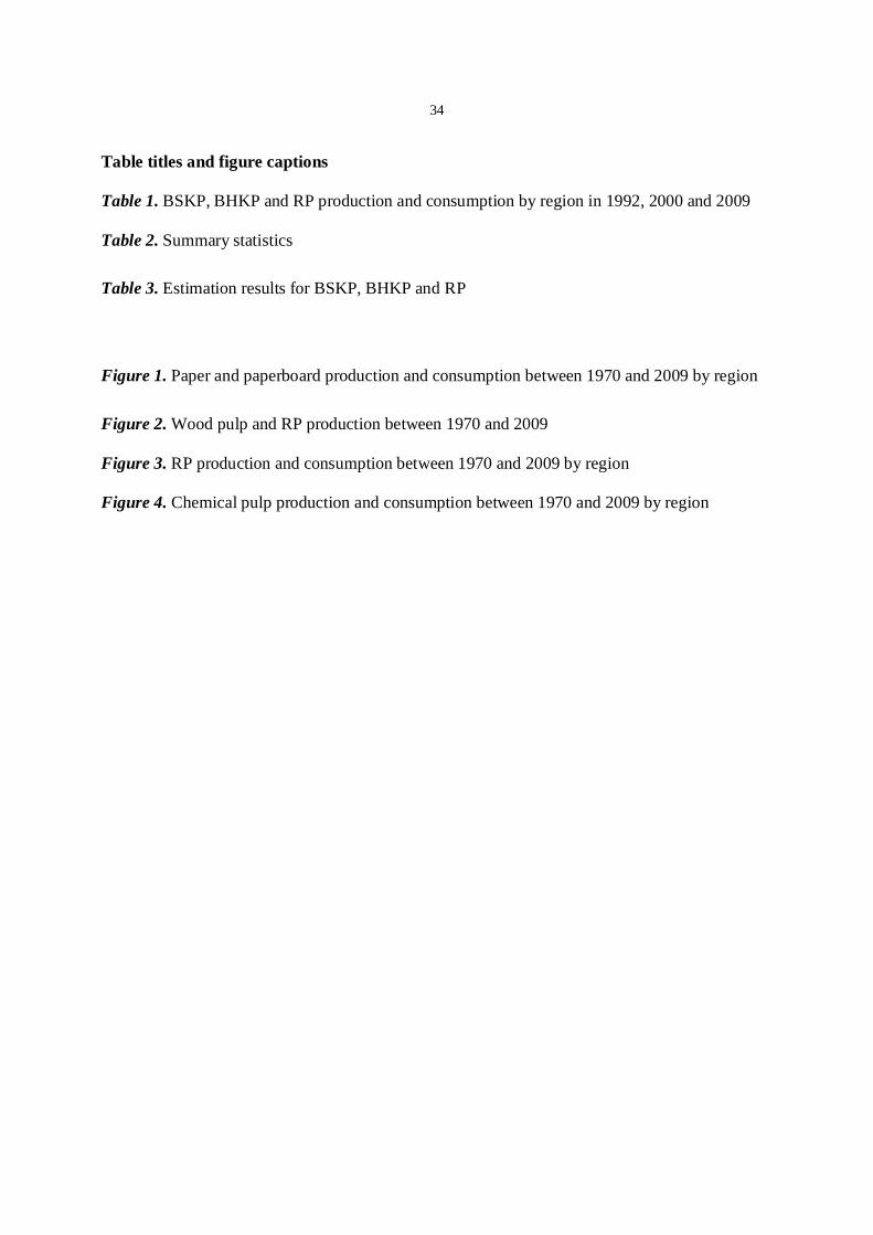
Table titles and figure captions
Table 1. BSKP, BHKP and RP production and consumption by region in 1992, 2000 and 2009
Table 2. Summary statistics
Table 3. Estimation results for BSKP, BHKP and RP
Figure 1. Paper and paperboard production and consumption between 1970 and 2009 by region
Figure 2. Wood pulp and RP production between 1970 and 2009
Figure 3. RP production and consumption between 1970 and 2009 by region
Figure 4. Chemical pulp production and consumption between 1970 and 2009 by region

35
Table 1. BSKP, BHKP and RP production and consumption by region in 1992, 2000 and 2009
(data source: RISI 2011a)
BSKP BHKP RP
1992 2000 2009 1992 2000 2009 1992 2000 2009
Production (% of world's total)
Asia 5 6 7 23 29 30 28 30 38
Europe 22 27 31 20 20 17 30 31 30
N. America 66 60 52 44 37 24 36 32 24
L. America 4 5 7 11 13 26 4 4 5
Other 2 2 2 2 2 2 2 3 4
Apparent consumption (% of world's total)
Asia 14 16 29 30 33 41 34 38 52
Europe 33 36 34 25 25 25 31 30 25
N. America 48 42 29 37 34 23 27 24 14
L. America 3 4 4 6 6 8 6 5 6
Other 2 2 3 2 2 2 2 3 3

36
Table 2. Summary statistics
Variable Mean Std. Dev. Min Max N
BSKP exports, tonnes 14.16 101.84 0.00 3 909.11 19 406
BHKP exports, tonnes 9.85 57.49 0.00 1 457.89 21 800
RP exports, tonnes 13.65 149.46 0.00 10 734.10 32 785
Distance, km 7 368.38 5 041.84 56.00 19 857.00 1 353
GDP (exporter), million USD 930 000 1 950 000 38 200 11 700 000 494
GDP (importer), million USD 550 000 1 420 000 9 380 11 700 000 1 026
GDP per capita (exporter), USD 18 901.28 11 119.93 592.10 41 900.79 494
GDP per capita (importer), USD 12 340.09 11 108.02 315.48 41 900.79 1 026
Population (exporter), millions 56.00 71.70 3.05 304.00 494
Population (importer), millions 85.60 212.00 1.97 1 320.00 1 026
Forest area (exporter), km2 920 031.10 1 960 098.00 20.00 8 092 690.00 75
Forest area (importer), km2 553 114.50 1 421 778.00 20.00 8 092 690.00 159
Consumer price index (exporter) 85.36 21.28 0.00 136.42 472
Consumer price index (importer) 78.68 29.13 0.00 177.33 992
Nominal exchange rate (exporter) 374.28 1 532.13 0.00 10 260.85 403
Nominal exchange rate (importer) 306.41 1 303.87 0.00 10 260.85 898

37
Table 3. Estimation results for BSKP, BHKP and RP
Model 1 (BSKP)
Model 2 (BSKP)
Model 3 (BHKP)
Model 4 (BHKP)
Model 5 (RP)
Distance -6.768 -5.720 -2.702 -4.968* -4.652*** (-0.89) (-0.32) (-1.09) (-1.71) (-5.33) GDP per capita (exporter) -0.831** -0.759** -0.103 -0.113 0.312 (-2.23) (-2.03) (-0.30) (-0.33) (0.87) GDP per capita (importer) 1.619*** 1.588*** 1.226*** 1.278*** 1.564*** (6.80) (6.66) (4.08) (4.20) (8.08) Population (exporter) -0.457 -0.850 1.010 0.837 -1.438*** (-0.42) (-0.76) (1.27) (1.04) (-2.66) Population (importer) 1.513*** 1.511*** -0.279 -0.341 0.984*** (2.84) (2.84) (-0.39) (-0.48) (3.31) Forest area (exporter) 6.098** 11.451*** -1.629*** -1.803*** (2.05) (2.82) (-3.51) (-3.76) Forest area (importer) -1.862*** -1.818*** 2.012*** 2.113*** -0.162 (-4.29) (-4.19) (3.35) (3.48) (-1.11) Real exchange rate 0.091 0.109 0.462*** 0.461*** -0.863*** (0.93) (1.11) (3.82) (3.79) (-7.51) North America (exporter) -1.034 -11.157 8.527*** (-0.09) (-0.44) (5.05) Latin America (exporter) 10.557 10.627 (0.70) (0.31) Northern Europe (exporter) 4.333 7.729 -2.103* (0.56) (0.45) (-1.69) Planted forest (dummy) -1.982 -1.897 (-1.12) (-1.06) China (importer) 10.376 9.056 -0.465 0.763 4.924** (0.56) (0.22) (-0.08) (0.12) (2.24) Decade dummy -0.546*** -0.631*** -0.681*** -0.675*** 0.489*** (-4.16) (-4.56) (-7.81) (-7.69) (7.42) Decade dummy 0.266* 0.358** -0.865*** * N. America (1.81) (2.32) (-9.93) Decade dummy 0.187 0.495 * L. America (0.61) (1.44) Decade dummy 0.971*** 1.023*** -0.680*** * N. Europe (7.54) (7.79) (-7.47) Decade dummy 0.391*** 0.393*** * Planted forest (4.02) (4.03) Decade dummy 1.122*** 1.128*** 1.028*** 0.984*** 1.439*** * China (4.88) (4.91) (3.91) (3.70) (7.37) Constant -28.798 -101.064 1.698 25.826 27.549* (-0.47) (-0.68) (0.06) (0.84) (1.95) Observations 3249 3249 3355 3355 5084 Number of groups 295 295 362 362 573 Hausman test FE vs. HT 3.71 0.28 4.09 2.57 11.02 chi2(12) chi2(12) chi2(10) chi2(10) chi2(8) Hausman test HT vs. RE 29.35** 33.45*** 63.00*** 64.44*** 101.6*** chi2(17) chi2(17) chi2(13) chi2(13) chi2(12) z statistics in parentheses (* significant at 10%; ** significant at 5%; *** significant at 1%)
38
Figure 1. Paper and paperboard production and consumption between 1970 and 2009 by region

39
Figure 2. Wood pulp and RP production between 1970 and 2009

40
Figure 3. RP production and consumption between 1970 and 2009 by region

41
Figure 4. Chemical pulp production and consumption between 1970 and 2009 by region