Explanation-based generalisation = partial evaluation

ARTIFICIAL INTELLIGENCE 401

RESEARCH NOTE

Explanation-Based Generalisation = Partial Evaluation*

Frank van Harmelen and Alan Bundy Depar tmen t o f A . I . , Universi ty o f Edinburgh , 80 South Bridge,

Edinburgh EH1 1HN, Scotland, United Kingdom

Recommended by M. Bruynooghe and T. Mitchell

ABSTRACT

We argue that explanation-based generalisation as recently proposed in the machine learning literature is essentially equivalent to partial evaluation, a well-known technique in the functional and logic programming literature. We show this equivalence by analysing the definitions and underlying algorithms of both techniques, and by giving a PROLOG program which can be interpreted as doing either explanation-based generalisation or partial evaluation.

I . Introduction

An interesting development in the field of machine learning is the advent of a technique called explanation-based generalisation (EBG). This name was first coined by Mitchell et al. [11] but the technique can be traced back to Mitchell [10], and earlier to DeJong [2] and Mitchell [9]. This technique tackles the problem of formulating general concepts on the basis of specific training examples. For some considerable time, the functional programming community, and more recently the logic programming community, has been discussing a technique called partial evaluation (PE) as a program optimisation method (see Futamura [5] for an early paper on PE, Ershov [4] for PE in functional programming, and Komorowski [8], Venken [18], and Takeuchi and Furukawa [16] for PE in logic programming). This paper shows that, in the context of logic programming, the two techniques, although developed for different purposes, do in fact consist of the same algorithm, and can both be im-

* The research reported in this paper was supported by SERC grant GR/44874.

Artificial Intelligence 36 (1988) 401-412 0004-3702/88/$3.50 (~) 1988, Elsevier Science Publishers B.V. (North-Holland)

402 F. VAN HARMELEN AND A. BUNDY

plemented by (almost) the same piece of code. This close resemblance between EBG and PE has not been noted before, and indeed, a number of papers (such as Prieditis and Mostow [13]), apparently treat EBG and PE as complementary techniques to achieve different goals, whereas in fact the two techniques are the same, as argued in this paper.

The rest of the paper is organised as follows: In Sections 2 and 3 we give brief descriptions of both EBG and PE. Section 4 paraphrases the definition of EBG to show that PE and EBG are essentially equivalent. Section 5 gives small implementations of both PE and EBG, and by comparing the two programs we see again that the two techniques are almost the same. Section 6 discusses the issue of guided versus unguided search that arises from the comparison of EBG and PE, and finally Section 7 gives a worked example often used in the EBG literature to show how the computation corresponds to PE.

2. Explanantion-Based Generalisation

EBG is a technique to formulate general concepts on the basis of a specific training example. The EBG algorithm consists of two stages. In the first stage EBG analyses a single training example in terms of knowledge about the domain and the goal concept under study, and produces an explanation of why the training example is an instance of the goal concept. The resulting explanation structure is then used as the basis for formulating the general concept definition by generalising this explanation, i.e. abstracting it from the particular training example.

As input, the EBG algorithm expects the following items:

- goal concept: a definition of the concept to be learned; - training example : a specific instance of the goal concept; - d o m a i n theory: a set of rules to be used in explaining why the training

example is an instance of the goal concept; - operat ional i ty criterion: a predicate over concept definitions, specifying the

form in which the learned concept definition must be expressed; this criterion defines a set of easily evaluated predicates from the domain theory.

Given these four inputs, the task is to determine a generalisation of the training example that is a sufficient definition for the goal concept and that satisfies the operationality criterion. Reexpressing the goal concept in these terms will make it operational with respect to the task of efficiently recognising examples of the concept. It is assumed that the input definition of the goal concept does not satisfy the operationality criterion.

As mentioned above, the EBG algorithm is usually described as consisting of two stages:

EXPLANATION-BASED GENERALISATION 403

(1) Explain: Construct an explanation in terms of the domain theory that shows how the training example satisfies the goal concept definition. This explanation must be constructed so that each branch of the explanation structure terminates in an expression that satisfies the operationality criterion.

(2) Generalise: Determine a set of sufficient conditions under which the explanation holds, stated in terms that satisfy the operationality criterion. This is accomplished by regressing (back propagating) the goal concept through the explanation structure. The conjunction of the resulting expressions constitutes the desired concept definition. This is typically done using a modified version of the goal-regression algorithm described by Waldinger [19] and Nilsson [12].

These two steps can be summarised as follows: the first step creates an explanation structure that separates the relevant feature values of the input example from the irrelevant ones. The second step analyses this explanation structure to determine the particular constraints on these feature values that are sufficient for the explanation to apply in general.

If the language used for expressing the input predicates and rules is logic, then the first step (explanation) amounts to proving that the input example is indeed an instance of the goal concept, in such a way that all the leaves of the proof tree are operational predicates, while the second step consists of building a more general version of this proof that does not depend on any of the irrelevant feature values of the input example.

3. Partial Evaluation

The main goal of PE is to perform as much of the computation in a program as possible without depending on any of the input values of the program. The theoretical foundation for PE is Kleene's S-M-N theorem from recursive function theory [7, p. 342]. This theorem says that given any computable function f o f n variables, f = f ( x l , . . . , xn), and k (k ~< n) values a 1 . . . . . a k for x~ . . . . , xk, we can effectively compute a new function f ' such that

f'(Xk+l . . . . . Xn) = f ( a l , . . . , ak,Xk+l . . . . . Xn).

'The new function f ' is a specialisation of f, and is easier to compute than f for those specific input values. The PE algorithm can be regarded as the implementation of this theorem, and is in fact slightly more general in the context of logic programming: it allows not only that a number of input variables are instantiated, but also that these variables can be only partially instantiated to terms that contain nested variables. Furthermore, the PE algorithm allows k in the above theorem (the number of instantiated input variables), to be 0, that is, no input to f is specified at all. Even in this case the PE algorithm is often able to produce a definition of f ' which is equivalent to f but more efficient, since all the computations performed by f that are independent of the values of


the input variables can be precomputed in f ' . Thus, the PE algorithm takes as its input a function (program) definition, together with a partial specification of the input of the program, and produces a new version of the program that is specialised for the particular input values. The new version of the program will then be less general but more efficient than the original version.

The PE algorithm works by symbolically evaluating the input program while in the mean time trying to (1) propagate constant values through the program code, (2) unfold procedure calls, and (3) branching out conditional parts of the code. If the language used to express the input program is logic, then the symbolic evaluation of the program becomes the construction of the proof tree corresponding to the execution of the program.

As mentioned, a special case of PE is when none of the values for the input variables x L . . . . . x k are given (in other words, k = 0). In this case, the PE algorithm cannot do as much optimisation of the input program, and as a result the new program will not be as efficient. However, the new program is no longer only a specialisation of the original program, but indeed equivalent to it. Thus, in this way PE can be used as a way of reformulating the input program in an equivalent but more efficient way.

4. EBG = PE

It has been the reformulation of E B G in terms of logical deduction (as given by Kedar-Cabelli and McCarty [6]) which has made the definition of it precise enough in order to allow the comparison between EBG and PE. In order to see that the processes performed by E B G and PE as described above, although formulated in different contexts, are indeed the same when rephrased in terms of logic, we first identify the inputs of E B G with the inputs of PE.

- The goal concept of E B G corresponds to the name of the program to be partially evaluated.

- T h e domain theory consists of the clauses and facts that constitute the program to be partially evaluated.

- T h e operationality criterion corresponds to the criterion that PE uses to stop the symbolic construction of the proof tree.

The normal PE algorithm is hardwired to only stop the construction of this proof tree at axioms in the form of single predicates (unit clauses, or facts, in PROLOG terminology). However, as we shall see below, the PE algorithm can be trivially changed so that it becomes parametrised over the operationality definition.

- T h e training example of E B G corresponds to the values of the input variables x 1 , . . . , x k .

However, as described above, PE does not really need the values for these variables. Furthermore, as remarked in [11, p. 67], E B G does not really need the training example either. In E B G the training example is only used to guide


the algorithm through the relevant t ransformation of the goal concept, thereby reducing the search space for the explanation step, but it is not strictly necessary for the execution of this step. To facilitate the comparison of E B G and PE we can therefore assume for the momen t that no training example is given, but we will return to this point in Section 6. When no training example is given, the second step in the E B G algorithm becomes superfluous: it is no longer necessary to abstract away from the particular feature values of the training example.

Both algorithms now consist of only one step, namely constructing a proof tree for the goal concept ( E B G terminology) or input predicate (PE terminology) using the rules of the domain theory, such that the leaves of this tree are all operational predicates. The conjunctions of all these leaves then forms the "reformulat ion of the goal concept" ( E B G terminology) or the "more efficient p rogram" (PE terminology).

It is now clear that both E B G and PE take as their inputs a goal predicate, a domain theory and an operationali ty criterion, and reformulate the original definition of the goal predicate in terms of operat ional predicates using the domain theory to justify the reformulation. Both E B G and PE perform this reformulation by constructing a proof tree with the goal predicate as the root-node and only operat ional predicates at the leaves, with the rules of the domain theory constituting the proof steps inside the tree.

5. EBG = PE by Implementation

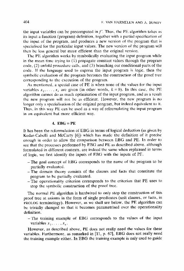
Figure 112gives the definition of a small partial evaluator for PROLOG prog rams .

peval(Leaf, Leaf):-clause(Leaf, true). peval((Goall, Goal2), (Leaves1, Leaves2)):-

peval(Goall, Leaves1 ), peval(Goal2, Leaves2).

peval(Goal, Leaves) :- clause(Goal, Clause), peval(Clause, Leaves).

Fig. 1. Partial evaluator.

1 Throughout this paper we use the standard Edinburgh syntax for PROLOG programs: variables start with uppercase letters or underscores, constants start with lowercase letters. As usual in Edinburgh syntax PROLOG systems, the predicate clause(Head, Body) searches through the clause set for a clause that unifies with Head :- Body backtracking over clauses in the clause set for multiple solutions.

2 This implementation of a partial evaluator only serves as illustrational purpose, and is barely of any practical value. To arrive at a practical partial evaluator, this program would have to be extended with facilities to deal with built-in predicates, and to avoid looping on recursive programs. However, the above program does illustrate the essential elements of the PE algorithm necessary for our discussion.


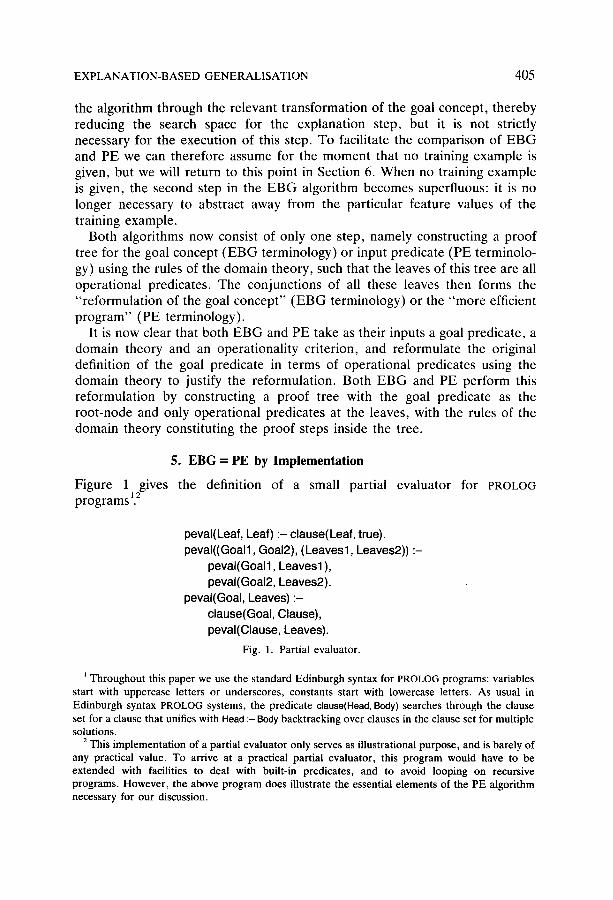
The predicate peval takes a predicate as its input in the first argument and symbolically simulates the execution of this predicate, returning the leaves of the resulting proof tree in the second argument. Notice that the other input to PE (the code of the program to be optimised) is implicit in the PROLOG database, using the clause-predicate). Not surprisingly, this partial evaluator looks very much like the standard PROLOG interpreter that it simulates. Figure 2 shows such a PROLOG interpreter in PROLOG.

prolog(Leaf) :- clause(Leaf, true). prolog((Goall, Goal2)) :-

prolog (Goal 1 ), prolog(Goal2).

prolog(Goal) :- clause(Goal, Clause), prolog(Clause).

Fig. 2. PROLOG interpreter.

The main difference between peval and prolog is that peval also returns the set of leaves of the proof tree as the result of the computation, thereby providing a reformulation of the input predicate in terms of the leaves of the tree.

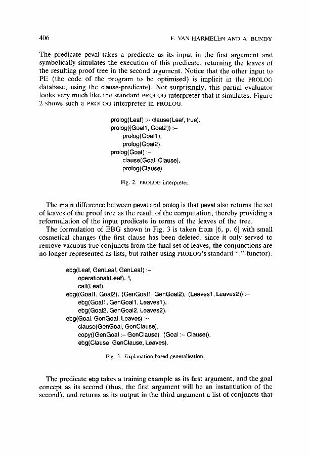
The formulation of EBG shown in Fig. 3 is taken from [6, p. 6] with small cosmetical changes (the first clause has been deleted, since it only served to remove vacuous true conjuncts from the final set of leaves, the conjunctions are no longer represented as lists, but rather using PROLOG's standard ","-functor).

ebg(Leaf, GenLeaf, GenLeaf) :- operational(Leaf), !, call(Leaf).

ebg((Goall, Goal2), (GenGoall, GenGoal2), (Leaves1, Leaves2)) :- ebg(Goall, GenGoall, Leaves1 ), ebg(Goal2, GenGoal2, Leaves2).

ebg(Goal, GenGoal, Leaves) :- clause(GenGoal, GenClause), copy((GenGoal :- GenClause), (Goal :- Clause)), ebg(Clause, GenClause, Leaves).

Fig. 3. Explanation-based generalisation.

The predicate eb9 takes a training example as its first argument, and the goal concept as its second (thus, the first argument will be an instantiation of the second), and returns as its output in the third argument a list of conjuncts that


form the leaves of the proof tree for the goal predicate. Again, certain parts of the input to ebg are implicit: both the domain theory and the operationality criterion are provided from the PROLOG database rather than being given as explicit arguments. As is clear from comparing Figs. 1 and 3, the EBG and PE code are very similar. They differ only in two small respects: the ebg code uses an explicit operationality criterion to stop the construction of the branches of the proof tree, whereas peval only stops when it finds unit clauses. The peval code can be trivially changed to taken an explicit operationality criterion into account, by changing the first clause of Fig. 1 into

peval(Leaf, Leaf) : - operational(Leaf), !, call(Leaf).

and then supplying an appropriate definition of operational. The second and more important difference between peval and ebg is the fact

that peval includes the unification with operational predicates in the conjuncts it returns, thereby restricting the reformulation of the goal concept, eb9 on the other hand takes care not to include these unifications in the resulting set of operational leaves. The extra second argument of ebg is intended to perform exactly this role: the first and second argument of ebg maintain exactly the same proof tree, but for the unifications with operational predicates in clause 1, which are not included in the third argument, which contains the final set of leaves. Leaving out the unifications of operational predicates at the leaves of the proof tree corresponds to the generalisation step of the EBG algorithm. In the words of Kedar-Cabelli and McCarty [6, p. 5]:

The generalization is formed by propagating rule substitutions but ignoring fact substitutions when creating proof tree.

However, the code for peval can be trivially changed to disregard unifications with operational predicates using the standard double-negation technique in PROLOG to avoid variable bindings from successful goals. The updated version of clause 1 of the code for peval above has to be changed into

peval(Leaf, Leaf) : - operational(Leaf), !, not not call(Leaf).

A final difference between the code for ebg and pevat to do with the generalisation process is the use of copy in the third clause of ebg. The role of the espy predicate is to ensure that the generalised tree exactly mirrors the specific tree, by having GenGoal :-GenClause and Goal :-Clause be exact copies, with new variables. However, as argued above, it is not really necessary


to provide the EBG algorithm with a training example. Therefore we do not have to maintain two separate versions of the proof tree, one specific and one general version, but we only need the general proof tree, and we can remove the copy predicate from the code of ebg.

After these rather trivial changes, the remaining differences between the formulations of peval and ebg are purely cosmetic, showing that they are indeed the same algorithm.

6. The Provision of a Training Example

As already mentioned above, EBG is usually described as needing a training example for the reformulation of the goal concept, but this training concept is not really necessary for the execution of EBG. The only purpose it serves is to restrict the number of possible reformulations of the goal concept by guiding the search through all possible rules from the domain theory. Although this reduction in the search space for the EBG algorithm is clearly desirable, there is a rather high price to be paid for this. The resulting reformulation of the goal concept is no longer equivalent to the original definition, but only represents sufficient (but possibly unnecessary) conditions for an example to be an instance of the goal concept. In [11, p. 57] this problem of sufficient-but- unnecessary conditions is mentioned as a topic for further research. However, as the comparison of EBG with PE shows, this problem can be solved by simply giving no training example at all. The S-M-N theorem then ensures us that the resulting reformulation will be equivalent to the original goal concept. Of course the computation is no longer guided by a target example, and is therefore much more expensive. Only when we are interested in just one special case is it still useful to provide a training example.

7. Worked Example

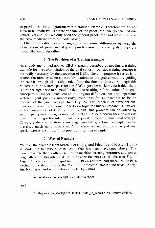
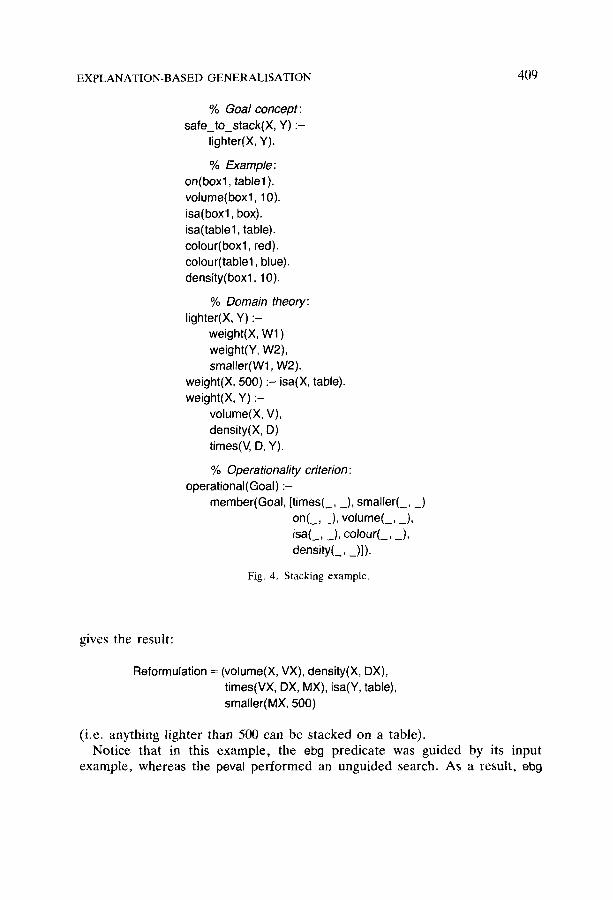
We take the example from Mitchell et al. [11] and Prieditis and Mostow [13] to illustrate the behaviour of the code that has been developed above. This example is one that is often used in the machine learning literature, and comes originally from Borgida et al. [l]. Consider the PROLOG database in Fig. 4. Figure 4 includes the full input for the EBG algorithm (and therefore for PE), excluding the definitions of the "built-in" predicates smaller and times. Apply- ing both peval and eb9 to this example, by calling

?- peval(safe to stack(X, Y), Reformulation).

and

?-ebg(safe to stack(boxl,tablel), safe to stack(X, Y), Reformulation).


% Goal concept: safe_to_stack(X, Y) :-

lighter(X, Y).

% Example: on(box1, table1 ). volume(box1, 10). isa(boxl, box). isa(tablel, table). colour(boxl, red). colour(tablel, blue). density(box1, 10).

% Domain theory: lighter(X, Y) :-

weight(X, Wl ) weight(Y, W2), smaller(W1, W2).

weight(X, 500) :- Jsa(X, table). weight(X, Y) :-

volume(X, V), density(X, D) times(V, D, Y).

% Operationafity criterion: operational(Goal) :-

member(Goal, [times(_, _), smaller(_, _) on(_, _), volume(_, _), isa(_, _), colour(_, _), density(_, _)]).

Fig. 4. Stacking example.

gives the result:

Reformulation = (volume(X, VX), density(X, DX), times(VX, DX, MX), isa(Y, table), smaller(MX, 500)

(i.e. anything lighter than 500 can be stacked on a table). Notice that in this example, the eb9 predicate was guided by its input

example, whereas the peval performed an unguided search. As a result, eb9


only computes the above reformulation of the goal criterion, whereas the unguided computation performed by peval also returns the following two reformulations:

Reformulation = (isa(X, table), volume(Y, VY), density(Y, DY), times(VY, DY, MY), smaller(500, MY))

(i.e. a table can be stacked on anything heavier than 500).

Reformulation = (volume(X, VX), density(X, DX), times(VX, DX, MX), volume(Y, VY), density(Y, DY), times(VY, DY, MY), smaller(MX, MY))

(i.e. anything can be stacked on anything lighter). These three formulations are generated by the two definitions of weight in

the domain theory. Since this definition is used twice (in the predicate lighter), we would potentially get four reformulations of the goal concept, but the fourth formulation would involve stacking two tables, both with weight 500, making the operational predicate smaller false. The fourth reformulation is therefore rejected. In this small example it is easy to see that the disjunction of all four alternative reformulations forms exactly the set of leaves of the fully expanded proof tree for a proof of the goal concept. This shows that PE gives a full equivalent reformulation of the goal concept (namely the disjunction of all four alternative reformulations), while EBG (guided by its example), only gives a reformulation whose conditions can in general be too strong.

8. Conclusions

After having given a general description of explanation-based generalisation and partial evaluation, we have used a specific formulation of both of them in terms of logical deduction to show that the two algorithms are essentially equivalent, modulo a few minor differences to do with the stop criterion and with the way the two formalisms treat unifications arising from leaves in the proof tree.

In general we believe that such rational reconstructions of apparently unrelated algorithms in terms of each other is a useful activity, not only because it prevents reinventing the wheel, but also because often such rational reconstructions generate new insights in and additions to both versions of the algorithm. In this case, both EBG and PE benefit from the comparison:

- It becomes clear that EBG consists strictly of a deductive reformulation of the original goal concept in terms of operational concepts.

- T h e comparison with PE shows us that there is no reason why the training example of EBG should be a ground term, although this is suggested by all the examples in the papers on EBG referred to above.


- In fact, as argued in Section 6 above, a training example is not necessary at all for EBG. This means that a balance can be struck between the cost of the search during the learning algorithm (high when no training example provided) and the generality of the concept that is learned (more general when no training example is provided).

- T h e r e is no strict need for PE to unfold the full proof tree all the way to the final leaves, but it is possible to stop this process at previously specified predicates, as defined by an explicit operational criterion. This insight is important because it might be used in solving two of the major problems associated with PE, namely firstly the termination of unfolding recursively defined predicates (it is not clear when to stop the potentially infinite unfolding of these predicates), and secondly the increase in size of the code after partial evaluation (this often exponential increase is due to the unfolding of all the conditional branches in the code).

- The current work on extending E B G to deal with imperfect (incomplete or inconsistent) theories (as mentioned in for instance [3, 15]) might have interesting implications for the logic programming community.

- The same holds for the work of Utgoff and others [17], showing that E B G leads to inventing "new" predicates, that were not explicit in the original domain theory.

- A lot of current work in the PE field, in particular on the possibilities of rejoining conditional branches and on heuristic guidance to the PE algorithm will be of similar interest to workers in explanation-based machine learning.

N o t e

After this paper had been provisionally accepted for publication, it was brought to our attention that similar results have been achieved simultaneously and independently by Prieditis [14].

REFERENCES

1. Borgida, A., Mitchell, T.M. and Williamson, K.E., Learning improved integrity constraints and schemas from exceptions in data and knowledge bases, in: M.L. Brodie and J. Mylopoulos (Eds.), On Knowledge Base Management Systems (Springer, New York, 1985).

2. DeJong, G., Generalizations based on explanations, in: Proceedings 1JCAI-81, Vancouver, BC (1981) 67-69.

3. Doyle, R., Constructing and refining causal explanations from an inconsistent domain theory, in: Proceedings AAAI-86, Philadelphia, PA (1986) 538-544.

4. Ershov, A.P., Mixed computation: Potential applications and problems for study, Theor. Comput. Sci. 18 (•982) 41-67.

5. Futamura, Y., Partial evaluation of computation process--an approach to a compiler-compiler, Syst. Comput. Control 2 (5) (1971) 45-50.

6. Kedar-Cabelli, S. and McCarty, L.T., Explanation-based generalization as resolution theorem proving, in: P. Langley (Ed.), Proceedings Fourth International Machine Learning Workshop,


lrvine, CA (1987) 383-389; also: Research Rept. No. ML-TR-10, Laboratory for Computer Science Research, Hill Center for Mathematical Sciences, Rutgers University, New Brun- swick, NJ.

7. Kleene, S., Introduction to Metarnathematics (Van Nostrand, New York, 1952). 8. Komorowski, H.J., Partial evaluation as a means for inferencing data structures in an

applicative language: A theory and implementation in the case of PROLOG, in: Proceedings Ninth Conference on the Principles of Programming Languages (POPL ), Albuquerque, NM (1982) 225-267.

9. Mitchell, T.M., Toward combining empirical and analytical methods for inferring heuristics, Tech. Rept. LCSR-TR-27, Laboratory for Computer Science Research, Rutgers University, New Brunswick, NJ (1982).

10. Mitchell, T.M., Learning and problem solving, in: Proceedings HCAI-83, Karlsruhe, F.R.G. (1983) 1139-1151.

l l. Mitchell, T.M., KelLer, R.M. and Kedar-Cabelli, S.T., Explanation-based generalization: A unifying view, Mach. Learning I (1) (1986) 47-81/; also Tech. Rept. ML-TR-2, Rutgers University, New Brunswick, NJ (1985).

12. Nilsson, N.J., Principles of Artificial Intelligence (Tioga, Palo Alto, CA, 19801. 13. Prieditis, A.E. and Mostow, J., PROLEARN: Towards a Prolog interpreter that learns, in:

Proceedings' AAA1-87, Seattle, WA (1987) 494-498; also: Research Rept. No. ML-TR-13, Lab. for Computer Science Research, Hill Center for Mathematical Sciences, Rutgers University, New Brunswick, NJ.

14. Prieditis, A.E., Environment-guided program transformation, in: Proceedings AAAI Spring Symposium, Stanford, CA (1988).

15. Rajamoney, S. and DeJong, G.. The classification, detection and handling of imperfect theory problems, in: Proceedings IJCAI-87, Milan~ Italy (19871 205-2//7.

16. Takeuchi, A. and Furukawa, K., Partial evaluation of Prolog programs and its application to recta programming, in: Proceedings 1FIPS-86, Dublin (1986) 415-420; also: ICOT Research Centre, Tech. Rept. TR-125, Tokyo (1986).

17. Utgoff, P.E. and Mitchell, T.M., Acquisition of appropriate bias for inductive concept learning, in: Proceedings AAAI-82, Pittsburgh, PA (19821 414-417.

18. Venken, R., A ProIog recta-interpreter for partial evaluation and its application to source transtk)rmation and query-optimisation, in: f'roceedings of ECAI-84, Pisa, italy (1984) 91-100.

19. Waldinger. R.. Achieving several goals simultaneously, in: Machine Intelligence 8 (Halstead and Wiley, New York, 1977) 94-138.

Received December 1987; revised version received May 1988

Documents

Explanation-based generalisation = partial evaluation